a markov chain model of the benefits of participating in government training schemes 1

A Markov Chain Model of the Benefits of Participating in Government Training Schemes*'

The Department of Employment's recent consultative document, Training fm the Future (HMSO 1972), inter alia announced the develop- ment of a new Training Opportunities Scheme, involving an expansion of the capacity of Government Training Centres (GTCs) and the greater use of colleges of further education and employers' facilities, with the aim of providing training, under the scheme, for not less than 60-70,000 persons by 1975 (a four-fold increase in five years), rising to a target figure of 100,OOO trainees a year. But what of those individuals who have already completed courses a t GTCs? In view of this massive expansion of Government training facilities it seems pertinent to inquire how far such courses have been worthwhile for those undertaking them in the past. The questions posed in this paper are: has participation in a GTC course led to higher incomes and, if so, have these been suffi- ciently high to offset any costs involved (in the form of income forgone) ?

The majority of (mainly American) studies concerned with similar issues have conducted comparative follow-up studies of both trainees and control groups. In this study, we make use of unpublished data collected by Ken Hall and Isobelle Miller during their follow-up study of GTC trainees in Scotlandz, to estimate earnings of trainees. The study, however, breaks new ground methodologically in presenting a stochastic model (in lieu of a control group) to assess retrospectively the labour market experiences of trainees, in the absence of training.3

Before turning to this model (in Section 2) and thence (in Section 3) to the results, the first section discusses the nature of monetary benefits and costs.

I. THE PRIVATE BENEFITS AND COSTS OF TRAINING

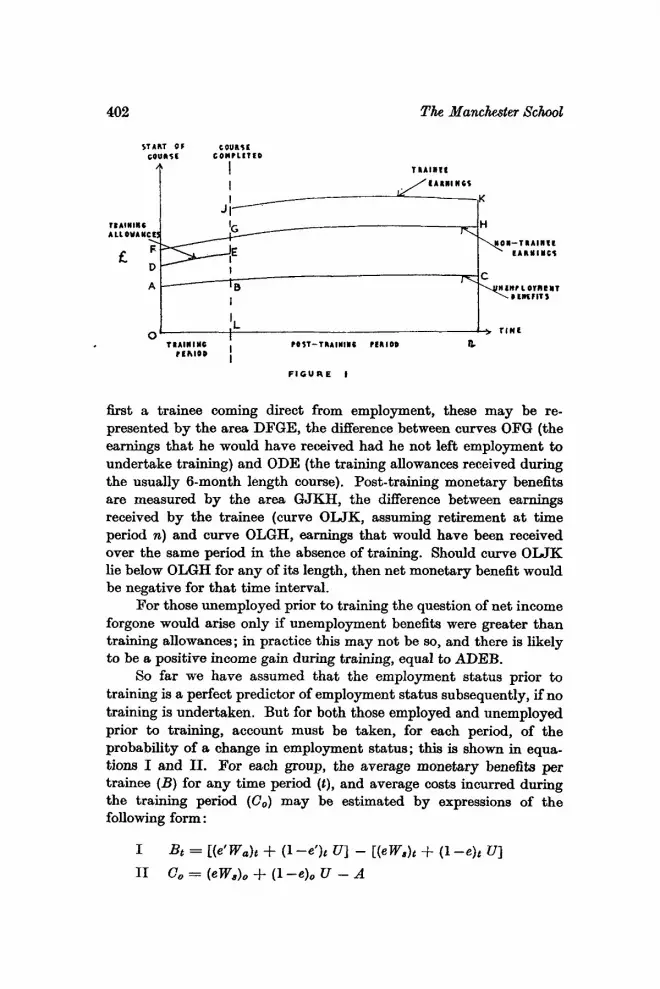
What are the monetary benefits and costs of participating in a GTC course? Noting that participants in GTCs are drawn both from the ranks of the unemployed and from employment, we may represent, initially, these private costs and benefits in Pigure 1.

Since the overt costs of training are borne by the Government, the participant costs are any net earnings forgone during training. Taking

*;Manuscript received 15.3.73; final version received 8.6.73. 401

402 The Manchester School

F I G U R E t

first a trainee coming direct from employment, these may be re- presented by the area DFGE, the difference between curves OFG (the earnings that he would have received had he not left employment to undertake training) and ODE (the training allowances received during the usually 6-month length course). Post-training monetary benefits are measured by the area GJKH, the difference between earnings received by the trainee (curve O U K , assuming retirement a t time period n) and curve OLGH, earnings that would have been received over the same period in the absence of training. Should curve OLJK lie below OLGH for any of its length, then net monetary benefit would be negative for that time interval.

For those unemployed prior to training the question of net income forgone would arise only if unemployment benefits were greater than training allowances; in practice this may not be so, and there is likely to be a positive income gain during training, equal to ADEB.

So far we have assumed that the employment status prior to training is a perfect predictor of employment status subsequently, if no training is undertaken. But for both those employed and unemployed prior to training, account must be taken, for each period, of the probability of a change in employment status; this is shown in equations I and 11. For each group, the average monetary benefits per trainee (B) for any time period ( t ) , and average costs incurred during the training period (C,) may be estimated by expressions of the following form :

1

I1 & = Ite‘FVah + (1 -e’h Ul - [(eWs)t + (1 -e)t l.Jl Co = (eW.,), + (1 -& U - A

A Harkov Chain Nodel 403

where ( Wa)t = actual earnings of trainees, in post training period, t (w& = earnings in the absence of training, in period t ( = earnings forgone during training period o

U = unemployment benefits A = GTC training allowance el-= probability of employment, for trainees e = probability of employment, for non-trainees

Then to compute the overall private profitabilities of participating in a GTC course, we may adopt (as in Section 3) standard investment appraisal techniques for comparing the s u m of these benefits and costs, over the time horizon that benefits and costs are thought to accrue.

How may equations I and I1 be estimated for each trainee group? Salary and employment information from the Hall-Miller follow-up survey for the 18-month period following training, enables us to estimate, directly or by extrapolation, Wa, WE and e’ over the time horizon following training. U and A may also be estimated by reference to the characteristics of the sample population and to scales of benefits and allowances. The crucial question, however, is: what would have been the employment characteristics of trainees in the absence of training? For each trainee group we need to know e, and et, th4 probability of being employed a t each time period; for these estimatm we turn to our simulation model, described in the following section.

2. TEE SINULATXON MODEL Unlike the situation depicted in Figure 1, which takes the em-

ployment status prior to training as a perfect predictor of subsequent labour force experience, we now recognise the fact that movements, or transitions, from unemployment to employment, and vice versa, will occur. Over time the pattern of those transitions may be extremely complicated.

Our central and simplifying assumption now is that the probability of change of employment status in a period is known and dependent only on the employment status in the preceding period; in particular, that the probabilities of movement from an unemployment state to employment, in a period, will differ according to the length of time already in unemployment. Assuming that the proceas of transition from one employment state to another, in each period, may be approxi- mated by a first order regular Markov chain, we may construct a matrix of transition probabilities (P), to describe this process (with a transition reading from row to column) :


u1 u2 u3 UL 0 1-a 0 0 a

1 - b 0 b 1-c c ]

where Ul (U2), (U3) represents the states: unemployed for up to

UL is a state of longer term unemployment (in excess of 3

E is an employment state and a, b, c, d and f are transition probabilities to be estimated.

The cells in the transition probability matrix (other than the h a 1 row and column) are defined in terms of length of unemployment as from the time origin (i.e. the start date of the GTC course). As time goes on, the unemployed move one period later either into the next unemployment state (except for the long term unemployed who remain in that state) or become employed. Since the probability of remaining unemployed in a time period is equal to unity minus the probability of becoming employed the former is defined if the latter is known; hence, only half of the transition probabilities need to be estimated directly, the others by subtraction. Those already employed will either move to the first unemployment state or remain employed. The probability (f) of leaving the employed state is assumed constant with length of time in employment (unlike the probability of leaving unemployment); this assumption is relaxed later.

Using a Rlarkov chain model of this kind, we may simulate for each period following the start of GTC course the total numbers that would be employed and unemployed in the absence of training. Total earnings in the absence of training may then be estimated by applying these results to known or estimated earnings data, as discussed earlier.

1, (2), (3) periods

periods)

Structural fwna of the model

notation : We now set out the model more formally, using the following

Unt : number of unemployed at time t , who have been unemployed

ULt : number of long-term unemployed a t time t .

UTt: total number unemployed a t time t = C Unt f ULt

for n periods.

N

fl-1

A Blarkov Chain Model 405

EO, :number in time t, of continuoilsly employed since initial

EEt : number of re-employed, in employment in time t. ETt : total number eniployed a t time t = EOt + Eel. pij : probability of moving from state i to stage j.

period.

At any time t , the states are as follows: Unemployed states : Ult, U2t . . . U N - 1 , UNt, ULt Employed states : Eot, EEt

Hence for any time t , we may define an employment status vector (L1) comprising aU possible labour force states in which an individual may be found :

Lt = [Ult, Uzt . . . ULVt, ULt, EEt, Eot]

The transition probability matrix P', assumed constant over time,

U1 U2 u3 . . . U N UL EE I30

is de6ned as follows:

U' 0 l-pU1EE 0 . . . 0 0 pUlEE 0 U2 0 0 l-pU2EE ... 0 0 p U2EE 0

U N [ 0 0 x . . _ 0 l - p U N P pUNEE 0 UL 0 0 0 . . . 0 I-pULE' PULEE 0 EE pEEUl 0 0 . . . 0 0 l-pEEU1 0 EO pEoUl 0 0 ... 0 0 0 l-pEoU1

It is noted that the model as now specified, contains two employment states, E O and EE. The definition of a separate state (EEt), into which the unemployed move once they have found a job, provides the opportunity of ascribing to it a somewhat higher probability of moving into Ut+l, than the probability of moving from EO, to Ult+l. The assumption here is that there is less likelihood of longer service em- ployees being made redundant than those who find new jobs after unemployment .4

An employment status vector for time t+l may be estimated from the transition probability matrix and vector Lt :

u2t+l, . . . . uNt+l, U L ~ , ~ , EEt+', Eot+,i

= [Ult, U2t, . . . . UNt, ULt, EEt, Eotl [ P I

[UT:+1, ET:+11 = [U%+l . - . . E O t + l l

3, AN APPLICATION TO GTC TRAINING IN SCOTLAND The Data

The model is now applied to GTC training in Scotland, utilizing data from the Hall-Miller survey of 258 Scottish GTC trainees, during 1968-71. It should be emphasised that much of these data, collected by Hall and Miller for purposes of consistency checking only, are rather incomplete for our purpose and it has proved impossible to collate data relating to the full sample. However, the analysis is largely intended as a pilot exercise in methodology-this to be applied to more robust data a t a later stage as noted below. Therefore it was felt justifiable to subject the data to less stringent requirements of accuracy than would normally be the case and the analysis proceeded on the basis that a sub- sample of available data was representative of the sample as a whole.

First, the cells in the transitional probability matrix (P) must be estimated and the initial state vector Lo constructed; then the details of estimation of the various incomes data required for the simulations are outlined.

Tra7Eeitional probability matrix: The model, aa run in this paper, contains a transitional probability matrix of seven states: five unemployment staka and the two employment states defbed above. Four unemployment states relate to periods of unemployment up to 3 ,6 ,9 and 12 months respectively; the long term unemployment state is defined as unemployment in excess of one year. Two alternative sets of transitional probabilities were used, to facilitate sensitivity testing of the h a 1 results to input assumptions made. A study of the unemployment register by Fowler (1968) was used for deriving probabilities giving a quicker response time and higher steady-state unemployment than a second set estimated on the basis of a study by MacKay (1972)

1 0 1 0 . . . . . . 1 0 0 1

- 0 1

A Markov Chain Model 407

of engineering worker redundancies. The Appendix outlines the method adopted for estimating these transitional probabilities and discusses the relative merits and defects of the two sets used.

Initial state vector (LO) : This gives the employment- unemployment status of trainees just prior to training. An estimate of the number of trainees in the unemployment states was made on the basis of the dates of previous employment (which was available for only one third of the sample). Similarly the number with no break in employment before entering the GTC was estimated. This figure was reduced by the 50 of those in ‘insecure employment’ who, in this initial analysis, were not considered further. The initial state vector was then constructed as :

Ulo Uzo Us0 Po ULo E E o EOo

Lo = [68 19 6 11 20 0 861

However, average results relating to all trainees may not be very useful or meaningful for the present private rate of return analysis (see Ziderman (1974) for a cost-benefit study dealing with societal rates of return). A potential trainee will be either unemployed or in a job and he wiU be interested only in the rate of return relevant to his particular status; hence we here compute separate rates of return for those out of a job and those employed, prior to training.5 We then have two initial state vectors, based on LO: for those unemployed, identical to LO except the cell EO is empty; all of the cells in the initial state vector for those continuously employed prior to training will be empty, except for EO (=85). Since two alternative transitional matrices are used there are, in all, four sets of simulations.

Act& earnings after training (e’Wa): The calculation of these earnings involved averaging over a variable sized sample at different points of time. The results in current prices are shown in Table 1, for the two trainee groups and for trainees as a whole. The figures shown for 18 months after training refer to dates of perhaps up to 2 years after training; as the exact date is in doubt, 18 months was used as an approximation. These data were corrected to real terms by relevant indices and extrapolated by an assumed annual real growth rate of 3%. The unemployment figures shown are based upon the unemployment percentages for a rather larger sample at each period. The unemployment figures by ‘employment status prior to training’ are assumed, on the basis of the known breakdown 18 months after training and the total sample figures for each period.

Assumed earnings in the absence of training ( W,) : For the wage rate of those in continuous employment (EO), that of the regularly employed

TAB

LE I

A

VE

RA

GE

EA

RN

ING

S A

ND

UN

EM

PLO

YM

EN

T OF G

TC

TR

AIN

EES

IN S

CO

TLA

ND

, B

Y E

MP

LOY

ME

NT

STA

TUS

PR

IOR

TO

TR

AIN

ING

, 19

68-7

1.

UN

EM

PLO

YE

D

EMPL

OYE

D

TOTA

L

Earn

ings

f 2

I *20

€2

0.80

f 1

9.20

€2

I *45

€2

3.75

N

o. o

bser

vatio

ns

I I6

44

70

72

73

% un

empl

oyed

-

40*0

* 9*

5*

8*5*

7.

5

% un

empl

oyed

-

30*0

* 6*

0*

5.0*

4.

0

% un

empl

oyed

-

36.4

7.

4 6.

6 5.

4

Earn

ings

f1

8.15

€2

1.05

€2

I*lO

€2

4.00

€2

7- I0

No.

obs

erva

tions

13

1 63

83

82

87

Earn

ings

€1

9.5

5 €2

0.95

€2

0.80

€2

2.80

€2

5.55

N

o. o

bser

vatio

ns

247

I07

I53

I54

I60

2 c3 t

Dat

a m

ay r

efer

to p

erio

d in

exc

ess

of 1

8 m

onth

s (s

ee t

ext)

. * A

ssum

ed (

see

text

).


prior to training was taken (shown in Table 1, Col. 1, together with the wage of those unemployed prior to training) but increased by 3% a year to reflect the secular increase in real wages. The same wage rate was assumed for the re-employed (EE), on the strength of the hding in the study by Daniels (1972) that the average real wage of Woolwich redundant workers in the new jobs had not changed significantly at the time of interview (typically two years after redundancy).

Training allowances ( A ) and unemployment benejits ( U ) : On the basis of prevailing rates and the number of dependents in the samples, an average training allowance and unemployment benefit was calculated respectively for those employed and those unemployed prior to training. As the allowances include fares and lodging grants, and the unemployment benefit figures do not include Earnings Related Supplement, it was necessary to modify the data intuitively. Training allowances were taken as €13.00 in both cases, unemployment benefit for those unemployed prior to training was taken a t E9.00 and for those employed prior to training at €10.00. No correction was made for any assumed increase over time on the assumption that training allowances and unemployment benefits though growing over time, remain constant in real terms.

The time-structure of the simulation: As data on actual post-training earnings were available only for some 18 months following training, simulated employment patterns and earnings were generated only for the training period and the following 18 months. For the period following this 18 months up to the chosen time horizon, unemployment for each class of workers is assumed to remain the same as after 18 months, and average earnings for each class of workers to grow in real terms at the same annual rate as incomes generally; a figure of 3 per cent was used as an estimate.

Investment Analysis To compute the overall private profitability of participation in a

GTC course, we adopt standard investment appraisal techniques for comparing benefits and costs over the time horizon considered (n periods), Three related profitability measures are used:

(i) the internal rate of return i.e. that rate of discount ( i ) which satisfies the following expression :

; Bt (l+i)-" - c, = 0 t-1


(ii) the net present value (PV) in money terms a t various rates of discount (r) :

n

t= l PV(E) = X Bt ( l+r) -n - C,

(iii) the benefit-cost ratio ( R ) at various rates of discount (r) :

R = C B: ( l+r) -n/C, n

:-1

One immediate issue arises: the time horizon to be considered. Actual earnings data of trainees are available for only some 18 months following completion of training and the unknown question, common to all studies of this type, is the pattern of earnings differentials over time. This issue is discussed in Ziderman (1969) where it is concluded that the usual assumption, of constant earnings differentials over the remaining working life of trainees, is unrealistic. Instead, we run the simulation on the basis of alternative time horizons, up to 10 years following the start of training. The advantage of this approach is not only in giving the reader the opportunity of making his own assumption with regard to the period over which benefits accrue, but also in demonstrating the sensitivity of the results, to length of time period considered.

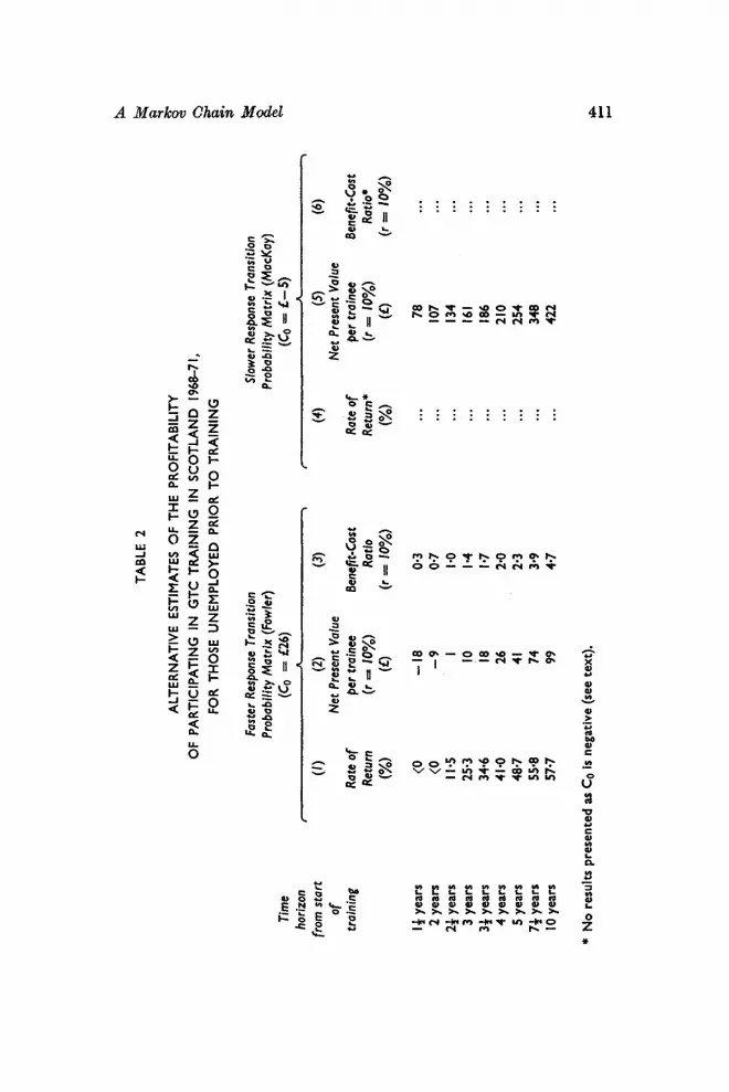
The major hdings are presented in Tables 2 and 3, respectively for those unemployed and those employed prior to training. Alternative results for each group are given, relating to quicker and slower unemployment transitional probability matrices (as discussed above and in the Appendix). The costs incurred during the usual six months course (C,) are shown at the head of the tables for each case. For those employed prior to training, costs are virtually identical (at 213.2) in the two simulations; those unemployed prior to training incur costs of ;E26 in one case but costs are negative in the second (i.e. training allowances exceed average earnings forgone), so that no rates of return or benefit cost ratios can meaningfully be presented for this case.

An interest rate of 10 per cent per annum is used for discounting future earnings to the present, to obtain net present values and the related benefit-cost ratios. The adoption of this high discount rate reflects the considerable uncertainty concerning the levels of future earnings. Since there is some doubt concerning the appropriate discount rate to be used, we aIso computed net present values using discount rates of 5% and 15%; since the general pattern of results was not found to be sensitive to discount rate variation, only results for the 10% case are shown.

TABL

E 2

b

ALTE

RN

ATIV

E ES

TIM

ATES

OF

THE

PRO

FITA

BILI

TY

OF

PAR

TIC

IPAT

ING

IN

GTC

TR

AIN

ING

IN

SC

OTL

AN

D 1968-71,

FOR

TH

OSE

UN

EMPL

OYE

D P

RIO

R T

O T

RA

ININ

G

Fast

er R

espo

nse

Tran

sitio

n Pr

obab

ility

Mat

rlx (F

owle

r) Ti

me

(Co

= f26)

horiz

on

I A

I

from

sta

rt (1

) (4

(3

) of

N

et P

rese

nt V

alue

tra

inin

g R

ate

of

per t

rain

ee

Bene

fit-C

ost

Ret

urn

(r =

10%

) R

atio

(%

I (f

) (I = fo

x)

I3 ye

ars

2 ye

ars

23 y

ears

3

year

s 33 ye

ars

4 ye

ars

5 ye

ars

73 y

ears

10

yea

rs

(0

(0

11.5

25.3

34.6

41.0

48.7

55.8

57.7

- 18

-9 I 10

18

26

41 74

99

0.3

0.7

I *o

I -4

I -7

2-0

2.3 3.9

4.7

Slow

er R

espo

nse

Tran

sitio

n Pr

obob

ility

Mat

rix (M

acKa

y)

(CO =

€-5

) ,

(4)

(4

(6)

Net

Pre

sent

Val

ue

Rat

e of

pe

r tra

inee

Be

nefit

-Cos

t R

etur

n*

(r =

10%

) R

atio

* (%

I (f

) (r

= 1

0%)

... 78

... ...

I 07

... ...

I34

... ...

161

... ...

I86

... ...

210

... ...

254

... ...

348

... ...

422

... * N

o re

sults

pre

sent

ed as

CO

is n

egat

ive

(see

text

).

Tim

e ho

rizon

fro

m s

tart

of

train

ing

I4 ye

ars

2 ye

ars

2t y

ears

3

year

s 34

year

s 4

year

s 5

year

s 7f

yea

rs

10 y

ears

TABL

E 3

ALT

ER

NA

TIV

E E

STIM

ATES

OF

THE

PR

OFI

TAB

ILIT

Y

OF

PA

RTI

CIP

ATI

NG

IN G

TC T

RA

ININ

G IN

SC

OTL

AN

D 1

968-

71

FOR

THO

SE E

MPL

OYE

D P

RIO

R T

O T

RA

ININ

G,

Fast

er R

espo

nse

Tran

sitio

n Pr

obab

ility

Mat

rix

(Fow

ler)

(Co =

€13

2

Slow

er R

espo

nse

Tran

sitio

n Pr

obab

ility

Mat

rix (M

acKa

y)

(Co =

€I 3

2)

(1)

(2)

(3)

Net

Pre

sent

Val

ue

Rate

of

per

train

ee

Bene

fit-C

ost

Ret

urn

(I =

10%

) R

atio

(I

= 1

0%)

(%I

(€1

<o

29.4

48. I

59.8

67.4

72.4

78

. I

826

83.5

- I6 34

82

I 27

171

212

289

452

58 I

0.9 1.3

I *6

20

2.3

2.6

3.2

4.

4 5.

4

(4)

(9

(6)

Net

Pre

sent

Val

ue

Rate

of

per

train

ee

Bene

fit-C

ost

Retu

rn

(I =

10%

) R

atic

(%

I (4

(r

= 1

0%)

I 4

32.5

51.3

63.0

70.5

75.4

81

.0 85

.4 86

.2

- I2 40

89

I36

I80

223

302

470

602

0.9

I *3

I *7

2.0

2.4

2.7

3.3

4.6 5 *6


From the foregoing tables, it is seen that a GTC course, within a year or two following the start of training, becomes a profitable private investment, in all cases. The results for those entering GTCs from unemployment (Table 2) are very sensitive to the values of the transitional probabilities assumed: the net present values for the slower employment response matrix (Column 5), are very considerably greater than those derived from that with faster employment response (Column 2)-for example, a trainee on average gains $186 in the latter case, compared with only $18 in the former, 3 years after completing training. Given the very low level of earnings forgone for this case, no great weight should be attached to the very high rates of return in Column 1. GTC training constitutes a more profitable investment for those joining the course direct from employment; as one would expect, the results of the two simulations in this case are very similar.

4. SIJMMABY AND CONCLUSIONS This paper has presented tentative estimates of the private net

monetary returns of participating in a course at a Government Training Centre, during 1968-1969. Average earnings ,following t.raining have been calculated from survey data relating to Scottish GTC trainees collected by K. Hall and I. Miller, at Heriot-Watt University; a stochastic simulation model has been developed (in lieu of the usual control group of non-trainees), to estimate the alternative average earnings in the absence of training. Separate results have been given for trainees joining the GTC course direct from a job and for those unemployed prior to training. A number of sensitivity testa have been applied but in all cases training emerges as a profitable private investment within two years, in some cases considerably sooner.

The research described in this paper is being extended in a number of directions. A recent retrospective survey by the Social Survey of the post-training careers of GTC trainees (Hunt, Fox and Bradley, 1972) makes available rather sounder data than used in this, mainly methodo- logical, paper; these new data are being re-analyzed to estimate returns to both society as a whole (in cost-benefit terms) as well as to individual trainees, by training trade and region. The Project’s own follow-up study of GTCs and control groups, now in the field, will provide, not only input data for calculating rates of return, collected specscally with this aim in view, but also the opportunity of coinparing results obtained from the control-group and the simulation methods, both relating to the same input data.

Queen Mary College (University of London)

ADRIAN ZIDERBUN and C. DRIVER

414 The Munchester School

APPENDIX

Estimation of the Transitional Probability Matrix The model as run in this paper contains a transitional probability

matrix with seven states : five unemployed states and two employment states. Four unemployment states are defined cumulatively in terms of lengths of 3 months and the long term unemployment state relates to unemployment in excess of 1 year. Hence the transitional probability matrix contains 14 elements, the following seven of which are to be estimated directly, the others by subtraction:

4 elements representing the probability of transition from unemployment state X (i.e. up to 3X months unemployment, X=l . . . a), to the re-employed state. The probability of transition to unemployment state X+l is obtained by subtraction.

-the probability of transition from long term unemployment to the re-employed state.

-the probability of transition from the regularly employed state to unemployed state 1.

-the probability of transition from the re-employed state to unemployment state 1.

We consider fust the latter two probabilities, from employed states. The rate of secondary unemployment from a re-employed state was found, in a study of redundancies among car workers in the London region in 1968, to be approximately 10 per cent for a two year period (Daniels, 1972). This figure was used to arrive at an estimate of 3% per three months, to correspond to the high unemployment rate in the Scottish region. A figure of half this was used for the probability of unemployment for those regularly employed. Although these figures can be regarded aa little better than ‘guestimates’, the final results are insensitive to fairly wide variations in their magnitude.

To estimate the transitional Probabilities of moving from an unemployed state into re-employment, we use as raw data a cumulative relative frequency curve, giving the percentage of unemployed who have obtained jobs after m months of unemployment (Cm). The transitional probabilities may be obtained from this curve by the expression :

where Pm, m+l is the probability of becoming employed between months m and m+ 1.

A Ma&m Chain Model 415

Fowler’s study of the unemployment register (Fowler, 1968) was used aa a basis for deriving these transitional probabilities. The Fowler study of various aspects of the unemployment register for the years 1961-65, contains an analysis of how the probability of going off the register during a given period varies over the length of unemployment. This is broken down by region and estimates of these probabilities are available for Scotland for these years.

Fowler’s analysis is only valid for the case of a stationary register i.e. one in which the overall level of unemployment is constant. Although these figures were updated (on a national basis only) to cover the period 1967-70, the lack of stationarity over these years causes doubt to be cast on the results. However, as a crude approximation to the data required for the model, transition probabilities were estimated by applying the same differential between the Scottish and national cumulate relative frequency curves of re-employment for 1961-65, to the 1967-70 national figures, thus obtaining a.n estimate of Cm applying in Scotland during the period under study. Cm was read a t values m=3, 6, 9 and 12 months, for which the transitional probabilities were calculated according to the foregoing formula. The final probability figure, that of transition out of long term unemployment, was set intuitively a t 30% per three month period.

It can be argued that a cohort of unemployed coming on the register are not typical of GTC trainees in many ways. Accordingly it was decided to observe the differences that would arise if a cohort of redundant workers were studied directly from the date of redundancy. Data are available from several case studies of this nature (e.g. Wedder- burn, 1965; MacKay 1972; Daniels, 1972) and it was found that all the cumulative relative frequency curves derived from these studies were below that of Fowler.

MacKay’s study of engineering worker redundancies in the Mid- lands waa used to derive a second set of transitional probabilities from an unemployed to a re-employed state, but with a slower response time and lower steady-state employment than those estimated from Fowler. C(m) for males was obtained from Table 3 in the paper, first corrected to exclude those obtaining first job immediately. The probability of transition out of long term unemployment was set a t 15%. It is questionable how applicable are the MacKay data, which refer to a level of unemployment half that of Scotland in the years of interest, since the characteristics of the Cm curve depend inter alia on the prevailing level of unemployment. (However, the average age of the MacKay sample was higher than that of trainees, an effect countering the influence of the unemployment rate). Although no firm basis

416 The Munchester School

exists for using the MacKay curve as model data it proved useful in demonstrating the sensitivity of the final results of our study to transition probability variation.

The h a 1 form of the two transitional probability matrices used are as follows:

UO v U2

P’(Fow1er) = U3 UL E E EO

UO U1 UZ

P’(MacKay) = P UL ES EO

uo UI uz u3

. 0 0-20 0 0 0 0 0.47 0 0 0 0 0.58 0 0 0 0 0 0 0 0

0.03 0 0 0 . 0.015 0 0 0

UL 0 0 0

0-66 0.70 0 0

E E 0.80 0.53 0.42 0.34 0.30 0.97 0

EO

0 0 0 0 0 0

0.985

uo U’ uz u3

. 0 0.42 0 0 0 0 0.55 0 0 0 0 0.54 0 0 0 0 0 0 0 0

0-03 0 0 0 ~ 0.015 0 0 0

UL 0 0 0

0-66 0.85 0 0

E E 0.58 0.45 0.46 0.34 0.15 0.97 0

EO 0 0 0 0 0 0

0-985

FOOTNOTES

1This paper represents part of a research project into the economics of Govern- ment Training Centres, fhanced by the Department of Employment. The project is located at Queen Mary College (University of London) and directed by A. Ziderman, Senior Lecturer in Economics, with the Research h i s t ance of C. Driver and Annamarie Walder.

2The study, directed by Ken Hall and undertaken a t the Department of Indus- trial Administration and Commerce, Heriot-Watt University, followed over an 18-month period the employment and earnings experiences of a sample of trainees who had participated in G.T.C. courses in Scotland during 1968 and early 1969. Some results are presented in Hall and Miller (1970A, 1970B, 1971). The unpublished earnings data used in the present paper were collected by the Heriot-Watt team as supplementary data for purposes of checking consistency; our thanks t o Ken H& for making these new date available.

Wtochastic models of the Markov chain type have been utilized increasingly in the manpower literature in recent years, studying such problems as labour mobility (Croasley, 1971), forecasting the grading structure in manpower systems (Bartholomew, 1970). mass redundancy (B. Curtis Eaton, 1970) and the opportunity costs of training (Ralph E. Smith, 1972). The model presented here has similarities in form and subject with the simpler ones presented in the latter two studies; it differs from its predeceasors in defining, more realistically, a number of transitional probabilities from unemployment to employment, dependant upon the length of time already unemployed (see text below).

4Since the state EO is one that cannot be entered from other states, the Markov chain is now non regular.

A Xarkov Chain Model 417

5It is recognised that computing average rates of return for all those unemployed prior to training meets the point only imperfectly since the recently unemployed do have a much better chance of finding a job quickly than the longer term unemployed (see transition probability matrices in the Appendix).

REFERENCES D. J. Bartholomew (1970), “Markov Chain Models for Manpower

Systems”, in A. R. Smith (ed.), Some Statistical Techniques in Manpower Planning, C.A.S. Occasional Paper No. 15, HMSO, 1970.

J. R. Crossley (1971), “A Mixed Strategy for Labour Economists”, Mimw, 1971.

W. W. Daniels (1972), Whtever happened to the workers in Woolwich?, Broadsheet 537, Political and Economic Planning, July 1972.

B. Curtis Eaton (1970), “Studying Mass Layoff through Markov Chains”, Industrial Relations, October 1970.

R. F. Fowler (1968), Duration of Unemployment on the Register of Wholly Unemployed, Studies in Official Statistics, Research Series No. 1, HMSO, 1968.

K. Hall and I. Miller (1970A), “Supplying Skills the Government Way”, Personnel Management, April 1970.

K. Hall and I. Miller (1970B), “The Adult Apprentice”, Industrial and Commercial Training, August 1970.

K. Hall and I. Miller (1971), “Industrial Attitudes to Skill Dilution”, British Journal of Industrial Relations, March 1971.

Audrey Hunt, Judith Fox and Michael Bradley (1972), Post Training Careers of Qovernment Training Centre Trainees, Office of Popula- tion Censuses and Surveys, €IMSO, 1972.

D. J. MacKay (1972), “After the ‘Shake-Out”’, Oxford Economic Papers, March 1972 (Vol. 24, No. 1).

Ralph E. Smith (1972), “The Opportunity Cost of Participating in B

!Graining Program”, Journal of H u m n Resources, Vol. VI, No. 4, 1972.

D. Wedderburn (1965), Redundancy and the Railwaymen, University of Cambridge, Department of Applied Economics, Occasional Paper No. 4, 1965.

A. Ziderman (1969), “Costs and Benefits of Adult Retraining in the UK”, EconomiCa, November 1969.

A. Ziderman (1974) “Cost Benefit Analysis of Government Training Centres in Scotland A Simulation Approach”, in J. M. Parkin and A. R. Nobay (eds.), Contemporary Issues in Economics: Proceedings of the Association of University Teachers of Economics Annual Conference, Warwick 1973, Manchester University Press, 1974.

a markov chain model of the benefits of participating in government training schemes 1

Documents