Manuscript ID TNN-2011-P-2933

1

Abstract— Implementation and new applications of a tunable

Complementary Metal–Oxide–Semiconductor Integrated Circuit

(CMOS-IC) of a recently proposed classifier Core-Cell (CC) are

presented and tested with two different datasets. With two

algorithms, one based on Fisher’s linear discriminant analysis

and the other on perceptron learning, used to obtain CC’s

tunable parameters, Haberman and Iris datasets are classified.

The parameters so obtained are used for hard-classification of

datasets with a neural network structured circuit. Classification

performance as well as coefficient calculation times for both

algorithms are given. The CC has 6 ns response time and 1.8 mW

power consumption. The fabrication parameters used for the IC

are taken from CMOS AMS 0.35 µm technology.

Index Terms—CMOS, Classifier, Fisher, Iris, Haberman

I. INTRODUCTION

LASSIFICATION is an important subject matter in many

applications ranging from pattern recognition, neural

networks to artificial intelligence, from statistics to template

matching [1], [2]. In general data classification can be realized

either by software or by hardware systems. Many algorithms

have been developed for classification [1]; however for faster

online operations on hard data it is desirable to realize these

classifiers in hardware which can be achieved with many

different approaches either in analog or digital domains.

Analog implementation of classification has many

advantages over digital ones. For one, complexity of analog

circuits is lower as compared to digital circuits; for another,

they can be built in voltage or current-mode (input and output

signals are current). In voltage-mode implementations the

supply voltage level has an important impact on the dynamic

range of the circuit. Current-mode approach provides larger

dynamic range for processing the variables. It is well known

that shrinking bias voltages makes it difficult to process data

in voltage-mode. A simple summing circuit, in voltage-mode,

needs additional active blocks (e.g. operational amplifiers and

additional circuitry); current-mode processing on the other

hand is preferred as currents can be added by connecting

output terminals of the blocks without requiring the use of

extra active blocks. For a handicap, the current-mode circuits

used to suffer from less accuracy in comparison to voltage-

Manuscript received January 25, 2011; revised June 15, 2011,October 20,

2011 and 01 February, 2012. This work is part of project 106E139 supported

by the Scientific & Technological Research Council of Turkey (TÜBİTAK). The authors are with the Department of Electronics and Communications

Engineering, Dogus University, Acibadem, Kadikoy 34722, Istanbul, Turkey.

(e-mail: cgoknar@dogus.edu.tr, myildiz@dogus.edu.tr, sminaei@dogus.edu.tr )

mode ones; but, in newer technologies (180 nm and below)

where low supply voltages are used, the accuracy in voltage-

mode circuits is also critical whereas current signals can

maintain high ratio accuracy [3]. Some classifier circuits,

using advantages of the current-mode approach, are listed in

the next paragraph.

For template matching applications, current-mode circuits

are proposed in [4] based on Euclidean distance calculator and

in [5] based on threshold circuits. Another current-mode

circuit which covers both Euclidean distance calculation and

Gaussian neighborhood tapering is given in [6]. A current-

mode sorting circuit for pattern recognition is designed to

build transformation between features and classes in [7] and

[8]. For pattern recognition applications a current-mode, fuzzy

IC is presented in [9]. Different classification solutions

regarding the implementation of neural networks on

programmable digital circuits and devices can be found in

[10], [11] but these circuits are relatively costly and high

power dissipating. A compact analog programmable multi-

dimensional radial basis function based classifier is proposed

in [12] and CMOS implementation of a Neural Network (NN)

classifier with several output levels and a different architecture

is given in [13]. CMOS realization of a conscience mechanism

used to improve the effectiveness of learning in winner-take-

all artificial neural networks, which also eliminates the dead

neurons, is presented in [14]. Except the one in [13], all these

circuits suffer from the shortcoming of not being tunable.

In this paper, the new DU-TCC 1209 IC containing 3 CCs,

9 Second-Generation Current Conveyors (CCII) and 3 current

buffers is being introduced. The newer CC architecture

published in [5], which improves the response time and the

Relative Tracking Error (RTE) as compared to the CC given

in [13], is being exploited in the IC design/layout/fabrication.

Connected properly, these CCs can be exploited to realize

n-D classifiers, which can only classify data, defined over

mesh-grid (rectangular partitioning) domains. To overcome

this deficiency, Linearly Weighting Circuits (LWC) that take

linear combinations of data and input these combinations to

CC are introduced as preprocessing units.

With two algorithms, modified/adapted versions of Fisher’s

Linear Discriminant Analysis (LDA) and Perceptron Learning

Algorithm (PLA) the weighting coefficients are calculated and

soft as well hard-tested on Iris and Haberman datasets.

Iris dataset consists of 50 samples from each of three

species of the Iris flowers, which are: virginica, versicolor and

setosa (3-class data). The flowers have 4 features which are

the lengths and widths of the sepal and petal in centimeters (4-

A Neural CMOS Integrated Circuit and

its Application to Data Classification

İzzet Cem Göknar, Fellow IEEE, Merih Yıldız, Member IEEE, Shahram Minaei, Senior Member

IEEE, and Engin Deniz, Member IEEE

C

Manuscript ID TNN-2011-P-2933

2

D data). This dataset is classified with LDA to distinguish the

flowers from each other [15]; the Iris dataset is not linearly

separable and is frequently used to test many other

classification techniques. Haberman dataset contains cases

from a study that was conducted between 1958 and 1970 at the

University of Chicago's Billings Hospital on the survival of

patients who have undergone surgery for breast cancer. It

consists of 306 samples from two classes, the patients who

survived 5 years or longer (255 samples) and the patients who

died within 5 years (81 samples). The dataset is 3-D with age

of the patient at the time of operation, patient’s year of

operation and number of positive axillary nodes detected.

The paper is organized as follows: in Section II, block

diagram, the transfer characteristic and the schematics of the

current-mode CC are given. In Section III, LWC needed for

datasets separated by hyperplanes with arbitrary slopes is

introduced. Derivation of parameter values for classifying

datasets using the modified Fisher’s LDA based algorithm is

given in section IV. The derivation of the same parameters

with PLA is given in section V. In Section VI, these weight

parameters are applied to the Iris and Haberman dataset

classifier circuits, which are constructed with LWCs and CCs;

also DU-TCC 1209 classification test results are compared

with the simulation results. Finally, Section VII concludes the

paper.

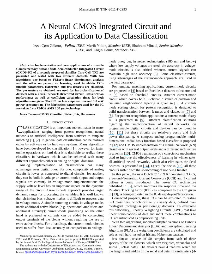
II. CMOS CORE CELL (CC)

The block diagram of the CC and its transfer characteristics

are shown in Figs. 1(a) and (b), respectively. The horizontal

position, the width and the height of the transfer characteristic

can be adjusted independently by means of external currents I1,

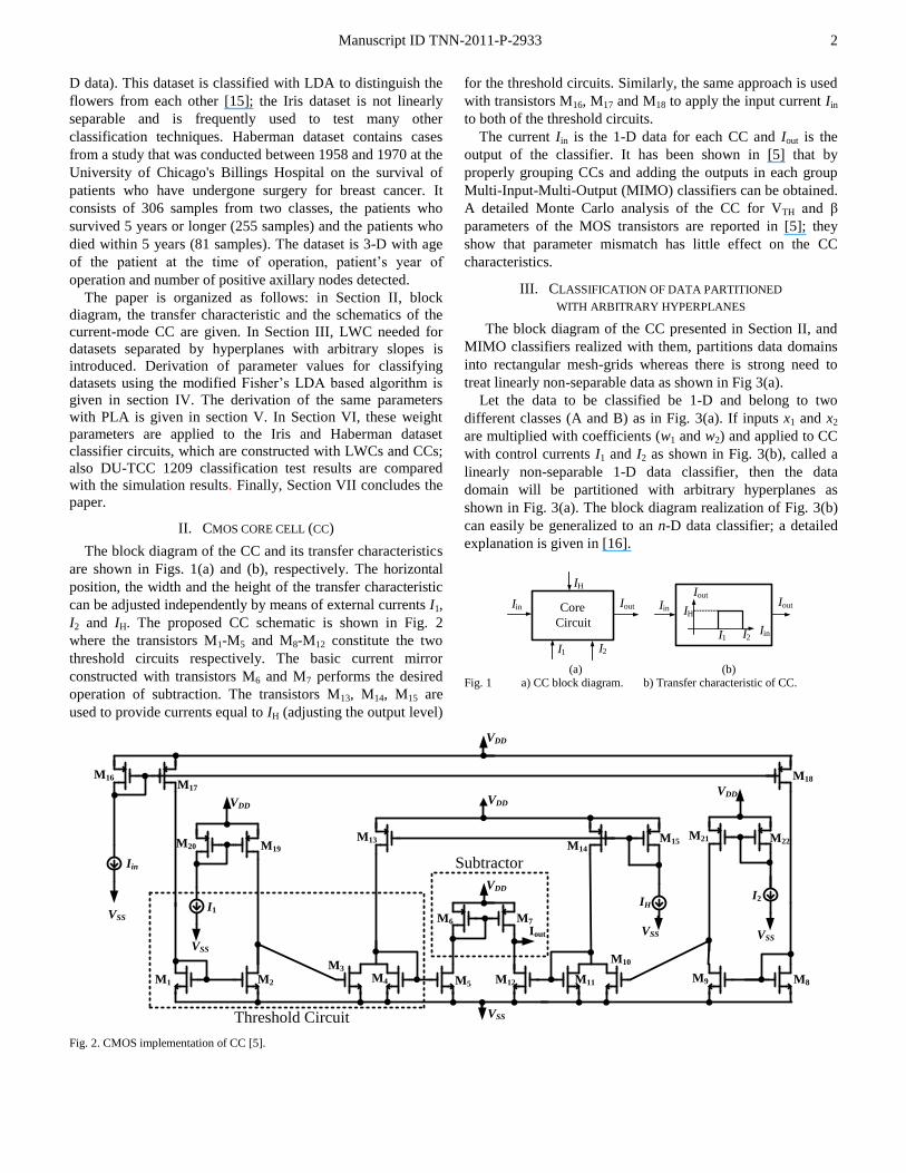
I2 and IH. The proposed CC schematic is shown in Fig. 2

where the transistors M1-M5 and M8-M12 constitute the two

threshold circuits respectively. The basic current mirror

constructed with transistors M6 and M7 performs the desired

operation of subtraction. The transistors M13, M14, M15 are

used to provide currents equal to IH (adjusting the output level)

for the threshold circuits. Similarly, the same approach is used

with transistors M16, M17 and M18 to apply the input current Iin

to both of the threshold circuits.

The current Iin is the 1-D data for each CC and Iout is the

output of the classifier. It has been shown in [5] that by

properly grouping CCs and adding the outputs in each group

Multi-Input-Multi-Output (MIMO) classifiers can be obtained.

A detailed Monte Carlo analysis of the CC for VTH and β

parameters of the MOS transistors are reported in [5]; they

show that parameter mismatch has little effect on the CC

characteristics.

III. CLASSIFICATION OF DATA PARTITIONED

WITH ARBITRARY HYPERPLANES

The block diagram of the CC presented in Section II, and

MIMO classifiers realized with them, partitions data domains

into rectangular mesh-grids whereas there is strong need to

treat linearly non-separable data as shown in Fig 3(a).

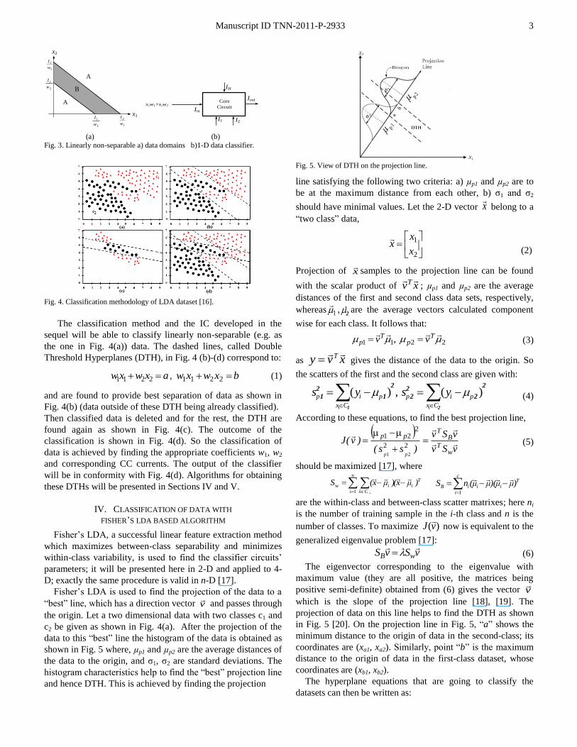
Let the data to be classified be 1-D and belong to two

different classes (A and B) as in Fig. 3(a). If inputs x1 and x2

are multiplied with coefficients (w1 and w2) and applied to CC

with control currents I1 and I2 as shown in Fig. 3(b), called a

linearly non-separable 1-D data classifier, then the data

domain will be partitioned with arbitrary hyperplanes as

shown in Fig. 3(a). The block diagram realization of Fig. 3(b)

can easily be generalized to an n-D data classifier; a detailed

explanation is given in [16].

IH

I1 I2

IoutIin Core

CircuitIin

Iout

I1 I2

IH

IoutIin

(a) (b) Fig. 1 a) CC block diagram. b) Transfer characteristic of CC.

I1

Iin

Iout

IHI2

VDDVDD

VDD

VDD

VDD

VSS

VSS

VSS

M1 M2

M3

M4 M5

M6 M7

M8M9

M10

M11M12

M13M14

M15

M16M17

M18

Threshold Circuit

VSS

M20 M19

M21 M22

VSS

Subtractor

Fig. 2. CMOS implementation of CC [5].

Manuscript ID TNN-2011-P-2933

3

x1

x2

1

1

w

I

1

2

w

I

2

1

w

I

2

2

w

I

A

A

B

x1w1+x2w2

IH

I1 I2

Iout

Iin

Core

Circuit

(a) (b)

Fig. 3. Linearly non-separable a) data domains b)1-D data classifier.

Fig. 4. Classification methodology of LDA dataset [16].

The classification method and the IC developed in the

sequel will be able to classify linearly non-separable (e.g. as

the one in Fig. 4(a)) data. The dashed lines, called Double

Threshold Hyperplanes (DTH), in Fig. 4 (b)-(d) correspond to:

axwxw 2211 , bxwxw 2211 (1)

and are found to provide best separation of data as shown in

Fig. 4(b) (data outside of these DTH being already classified).

Then classified data is deleted and for the rest, the DTH are

found again as shown in Fig. 4(c). The outcome of the

classification is shown in Fig. 4(d). So the classification of

data is achieved by finding the appropriate coefficients w1, w2

and corresponding CC currents. The output of the classifier

will be in conformity with Fig. 4(d). Algorithms for obtaining

these DTHs will be presented in Sections IV and V.

IV. CLASSIFICATION OF DATA WITH

FISHER’S LDA BASED ALGORITHM

Fisher’s LDA, a successful linear feature extraction method

which maximizes between-class separability and minimizes

within-class variability, is used to find the classifier circuits’

parameters; it will be presented here in 2-D and applied to 4-

D; exactly the same procedure is valid in n-D [17].

Fisher’s LDA is used to find the projection of the data to a

“best” line, which has a direction vector v

and passes through

the origin. Let a two dimensional data with two classes c1 and

c2 be given as shown in Fig. 4(a). After the projection of the

data to this “best” line the histogram of the data is obtained as

shown in Fig. 5 where, µp1 and µp2 are the average distances of

the data to the origin, and σ1, σ2 are standard deviations. The

histogram characteristics help to find the “best” projection line

and hence DTH. This is achieved by finding the projection

Fig. 5. View of DTH on the projection line.

line satisfying the following two criteria: a) µp1 and µp2 are to

be at the maximum distance from each other, b) σ1 and σ2

should have minimal values. Let the 2-D vector x

belong to a

“two class” data,

2

1

x

xx

(2)

Projection of x

samples to the projection line can be found

with the scalar product of xvT ; µp1 and µp2 are the average

distances of the first and second class data sets, respectively,

whereas 1

, 2are the average vectors calculated component

wise for each class. It follows that:

,11 T

p v 22 T

p v (3)

as xvy T

gives the distance of the data to the origin. So

the scatters of the first and the second class are given with:

( ) ,i

p i p

x C

s y

1

22

1 1 ( )i

p i p

x C

s y

2

22

2 2 (4)

According to these equations, to find the best projection line,

vSv

vSv

)ss()v(J

wT

BT

pp

pp

22

221

21

(5)

should be maximized [17], where

n

1iw

Ti

Cxi )μx()μx(S

i

c

i

TiiiB )μμ)(μμ(nS

1

are the within-class and between-class scatter matrixes; here ni

is the number of training sample in the i-th class and n is the

number of classes. To maximize )(vJ

now is equivalent to the

generalized eigenvalue problem [17]:

vSvS wB

(6)

The eigenvector corresponding to the eigenvalue with

maximum value (they are all positive, the matrices being

positive semi-definite) obtained from (6) gives the vector v

which is the slope of the projection line [18], [19]. The

projection of data on this line helps to find the DTH as shown

in Fig. 5 [20]. On the projection line in Fig. 5, “a” shows the

minimum distance to the origin of data in the second-class; its

coordinates are (xa1, xa2). Similarly, point “b” is the maximum

distance to the origin of data in the first-class dataset, whose

coordinates are (xb1, xb2).

The hyperplane equations that are going to classify the

datasets can then be written as:

Manuscript ID TNN-2011-P-2933

4

,x

xv

x

xv

a

aTT 02

1

2

1

02

1

2

1

b

bTT

x

xv

x

xv

(7)

The process is repeated for data between the hyperplanes, the

data outside being classified.

The components of the so chosen eigenvector determine the

weight coefficients (e.g. (14) in Section VI.B) to be used in the

LWC that will implement the separating hyperplanes.

In the n-D case, the only difference is in the dimension of

the involved matrices in (6), which is now n×n; again one has

to find the eigenvector, corresponding to the eigenvalue with

maximum value to determine DTH [18]-[20].

V. CLASSIFICATION OF DATA WITH THE

PERCEPTRON LEARNING ALGORITHM

The classical PLA widely used in neural networks is based

on a single threshold activation function [21] whereas the one

used here is double threshold function as shown in Fig. 1(b).

Regions separated by DTH are characterized by:

00

01

iTi

iTi

iavx

avxy

(8)

00

01

iTi

iTi

ibvx

bvxy

(9)

With the algorithm developed next for DTH, the vectors vi,

the DTH coefficients ai and bi in (8) and (9), relevant to the i-

th class, will be determined. Classification of the data will

then be achieved by separating the classes with appropriate

number of hyperplanes.

Perceptron Learning based Classification Algorithm

Selecting one of the data classes ci (i=1,2,..,m):

1. Check, if there is an appropriate DTH that separates all

data of class ci from all the others.

a. If there is, save these coefficients and delete this data

class from list; move to step 2.

b. If there is not, then move to step 3.

2. Continue with the remaining classes.

a. If the remaining class is m-th, then stop classification.

b. If not, move to the step 1.

3. Increase the number of DTH by 1 and check whether all

data from class ci can be separated from other classes.

a. If, yes then save the coefficients of DTHs and remove

this data class from list; move to step 2.

b. If, the class cannot be separated then move to step 3.

As the activation function is a hard limiter, the coefficients

can be calculated with the update rules of PLA [22] given

below.

Perceptron learning algorithm update rules:

(10)

(11)

(12)

In (10-12) yd and yo are the desired and the output obtained

at that step respectively; η is the learning coefficient which has

to be chosen between 0 and 1.While updating, when yd = yo the

weight coefficients do not change. Learning algorithm stops

when all weight coefficients stay constant [23].

When learning is finished using the training set, the DTHs

iTii bvxa

partition the data domain into regions each

containing a single class of data. Components of v

obtained

from the learning algorithm give the weight coefficients of

LWC, and ai and bi determine the CC’s control currents I1 and

I2. The remaining data set will be used to verify the correct

operation of the classifier so obtained. The CC current IH helps

to identify the class of the data. Thus, classification is

provided with appropriate number of LWC and CC blocks. In

the sequel both algorithms will be used to hard and soft-

classify Iris and Haberman datasets.

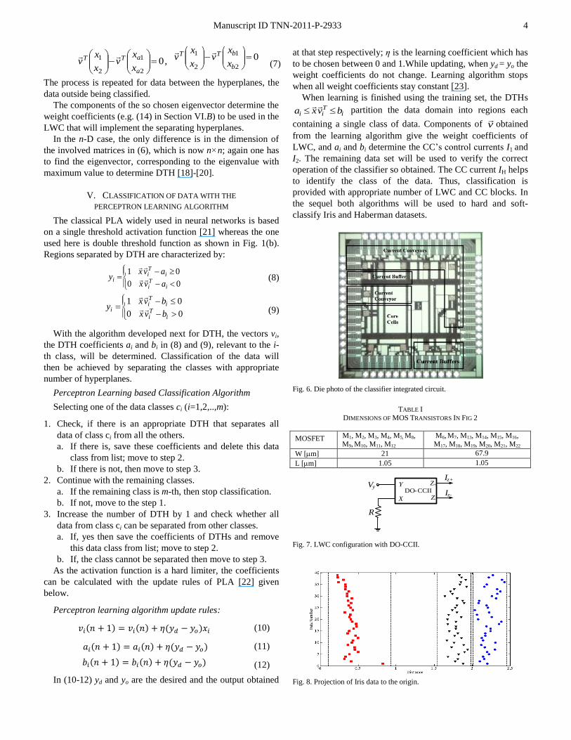
Fig. 6. Die photo of the classifier integrated circuit.

TABLE I DIMENSIONS OF MOS TRANSISTORS IN FIG 2

MOSFET M1, M2, M3, M4, M5, M8, M9, M10, M11, M12

M6, M7, M13, M14, M15, M16, M17, M18, M19, M20, M21, M22

W [m] 21 67.9

L [m] 1.05 1.05

Vy Y

X

Iz+

Iz-

R

DO- CCII

Z+

Z-

Fig. 7. LWC configuration with DO-CCII.

Fig. 8. Projection of Iris data to the origin.

Manuscript ID TNN-2011-P-2933

5

VI. REALIZATION OF THE CORE CIRCUIT, LINEARLY

WEIGHTING COEFFICIENTS AND TEST RESULTS

A. CMOS Realizations

The layout of the CC and of the IC including 3 CCs, 9

current conveyors and 3 current buffers have been designed

using MENTOR software with fabrication parameters for the

CMOS AMS 0.35 µm process [24]. The die photo of the

manufactured IC, called DU-TCC 1209, is shown in Fig. 6. In

order to provide user tunability all 52 pins had to be used for

I/O access, causing the pads dominate IC area, thus a pad

limited design. DU-TCC 1209 has a 2.62×2.62 mm2

die area

and CMOS transistors’ dimensions of the CC are given in

Table I.

The block diagram of the LWC using a Dual Output Second

Generation Current Conveyor (DO-CCII) [16] is shown in Fig.

7. The voltage Vy is the input and the current Iz+ and Iz- are the

outputs of the circuit in Fig. 7; these output currents can be

expressed as:

R

VI

yz

R

VI

yz

The resistance R is used to convert the voltage input data

Vy, to current; moreover, the ratio 1/R provides the appropriate

weight value for the realization. It is worthwhile mentioning

that the DO-CCII can also be used to provide negative weight

values using the Z- terminal in case the need arises.

B. Experimental Setting and Applications

The 4-D Iris dataset has 150 samples with equal number

from three classes (c1, c2, c3). Taking 40 data from each class

and using Fisher’s LDA, the coefficients of the projection

(eigen)vector are obtained as:

140100800570 ....v

. (14)

The projection of the Iris data using v

(the scalar product

xvT ) is shown in Fig. 8. It can be seen from Fig. 8 that the

data belonging to three different classes can be separated with

appropriate boundaries (DTH); these boundaries determine the

CC control currents. To test DU-TCC 1209 with the Iris data,

the classifier block diagram given in Fig. 9 was constructed on

a specially designed Printed Circuit Board (PCB) shown in

Fig. 10 where potentiometers provide tunability; in building

the classifier, product of Iris input data with the vector v

(wi

coefficients) was provided with LWC blocks as outlined next.

In order to obtain weighting coefficient w1 = 0.57 in (14) the

resistor R1 at the X terminal of the 1st DO-CCII is tuned to the

value R1 = 10/0.57 k providing an output current IZ+ =

0.57(V/10k). For the 2nd

coefficient w2 = 0.80 of (14), the

resistor R2 at the X terminal of the 2nd

DO-CCII is tuned to R2

= 10/0.80 k, providing an output current IZ- = 0.80(V/10k) to

secure the minus sign and so on.

To test the weight values provided by the algorithm, unused

30 data (10 from each class) was soft-applied to the classifier

of Fig. 9 with a 4-channel programmable-output function

generator. Each data was applied with 1 ms duration and was

classified correctly; the outcome is shown in Table II (only 20

shown because of space limitations).

LWC-1

x1

LWC-2x2

LWC-3x3

LWC-4x4

Current

Follower

CC-1

CC-2

CC-3

Output

x1w1

x2w2

x3w3

x4w4

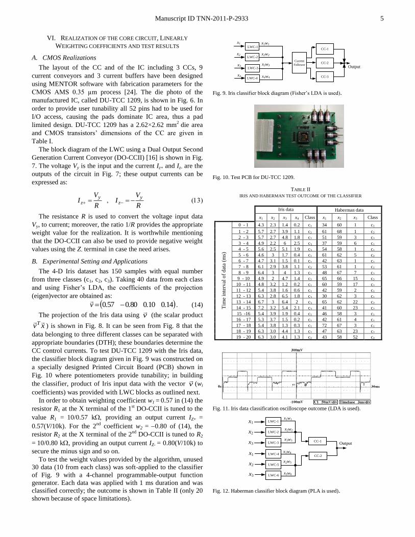
Fig. 9. Iris classifier block diagram (Fisher’s LDA is used).

Fig. 10. Test PCB for DU-TCC 1209.

TABLE II IRIS AND HABERMAN TEST OUTCOME OF THE CLASSIFIER

Iris data

Haberman data

x1 x2 x3 x4 Class x1 x2 x3 Class

Tim

e in

terv

al o

f d

ata

(ms)

0 - 1 4.3 2.3 1.4 0.2 c1 34 60 1 c1

1 - 2 5.7 2.7 3.9 1.1 c2 61 68 1 c2

2 - 3 5.7 2.7 4.8 1.8 c2 51 59 3 c2

3 - 4 4.9 2.2 6 2.5 c3 37 59 6 c1

4 - 5 5.6 2.5 5.1 1.9 c3 54 58 1 c1

5 - 6 4.6 3 1.7 0.4 c1 61 62 5 c2

6 - 7 4.7 3.1 1.5 0.1 c1 42 63 1 c1

7 - 8 6.1 2.9 3.8 1.1 c2 53 61 1 c1

8 - 9 6.4 3 4 1.3 c2 48 67 7 c2

9 - 10 4.9 2 4.7 1.4 c2 65 66 15 c2

10 - 11 4.8 3.2 1.2 0.2 c1 60 59 17 c2

11 - 12 5.4 3.8 1.6 0.6 c1 42 59 2 c1

12 - 13 6.3 2.8 6.5 1.8 c3 30 62 3 c1

13 - 14 6.7 3 6.4 2 c3 65 62 22 c2

14 - 15 7.2 3.2 5.4 2.1 c3 41 60 23 c2

15 -16 5.4 3.9 1.9 0.4 c1 46 58 3 c1

16 - 17 5.3 3.7 1.5 0.2 c1 42 61 4 c1

17 - 18 5.4 3.8 1.3 0.3 c1 72 67 3 c1

18 - 19 6.3 3.0 4.4 1.3 c2 47 63 23 c2

19 - 20 6.3 3.0 4.1 1.3 c2 43 58 52 c2

Fig. 11. Iris data classification oscilloscope outcome (LDA is used).

LWC-1x1

LWC-2x2

LWC-3x3CC-1

Output

LWC-4x1

LWC-5x2

LWC-6x3

CC-2

x1w1

x2w2

x3w3

x1w4

x2w5

x3w6

Fig. 12. Haberman classifier block diagram (PLA is used).

Manuscript ID TNN-2011-P-2933

6

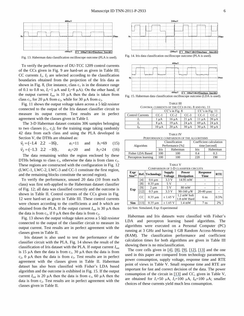
Fig. 13. Haberman data classification oscilloscope outcome (PLA is used).

To verify the performance of DU-TCC 1209 control currents

of the CCs given in Fig. 9 are hard-set as given in Table III;

CC currents I1, I2 are selected according to the classification

boundaries obtained from the projection of the Iris data as

shown in Fig. 8, (for instance, class c1 is in the distance range

of 0.1 to 0.8 so, I1=1 µA and I2=8 µA). On the other hand, if

the output current Iout is 10 µA then the data is taken from

class c1, for 20 µA from c2, while for 30 µA from c3.

Fig. 11 shows the output voltage taken across a 5 kΩ resistor

connected to the output of the Iris dataset classifier circuit to

measure its output current. Test results are in perfect

agreement with the classes given in Table I.

The 3-D Haberman dataset contains 306 samples belonging

to two classes (c1, c2); for the training stage taking randomly

42 data from each class and using the PLA developed in

Section V, the DTHs are obtained as:

)162.24.1(1 v

, a1=11 and b1=69 (15)

)102.23.1(2 v

, a2=20 and b2=24 (16)

The data remaining within the region enclosed by these

DTHs belongs to class c1, otherwise the data is from class c2.

These regions are constructed with the configuration in Fig. 12

(LWC-1, LWC-2, LWC-3 and CC-1 constitute the first region,

and the remaining blocks constitute the second region).

To verify the performance, unused 20 data (10 from each

class) was first soft-applied to the Haberman dataset classifier

of Fig. 12; all data was classified correctly and the outcome is

shown in Table II. Control currents of the CCs given in Fig.

12 were hard-set as given in Table III. These control currents

were chosen according to the coefficients a and b which are

obtained from the PLA. If the output current Iout is 30 µA then

the data is from c1, if 0 µA then the data is from c2.

Fig. 13 shows the output voltage taken across a 5 kΩ resistor

connected to the output of the classifier circuit to measure its

output current. Test results are in perfect agreement with the

classes given in Table II.

Iris dataset is also used to test the performance of the

classifier circuit with the PLA. Fig. 14 shows the result of the

classification of Iris dataset with the PLA. If output current Iout

is 15 µA then the data is from c1, 30 µA then the data is from

c2, 0 µA then the data is from c3. Test results are in perfect

agreement with the classes given in Table II. Haberman

dataset has also been classified with Fisher’s LDA based

algorithm and the outcome is exhibited in Fig. 15. If the output

current Iout is 20 µA then the data is from c1, 60 µA then the

data is from c2. Test results are in perfect agreement with the

classes given in Table II.

Fig. 14. Iris data classification oscilloscope outcome (PLA is used).

Fig. 15. Haberman data classification oscilloscope outcome (LDA is used).

TABLE III

CONTROL CURRENTS OF THE CCS IN FIG. 8 AND FIG. 11

CC’s in Fig. 8 CC’s in Fig. 11

Control Currents CC-1 CC-2 CC-3 CC-1 CC-2

I1 1 µA 16 µA 21 µA 11 µA 20 µA

I2 8 µA 19 µA 24 µA 69 µA 24 µA

IH 10 µA 20 µA 30 µA 30 µA 30 µA

TABLE IV

PERFORMANCE COMPARISON OF THE ALGORITHMS

Algorithm

Classification

Performance [%]

Coefficient calculation

time [second]

Iris Haberman Iris Haberman

Fisher LDA Based 100 100 0.4 0.3

Perceptron learning 100 100 220 190

TABLE V

COMPARISON OF 1-D CLASSIFIER CIRCUITS

Exp/

Sim(a) Ref. Technology

Supply

Voltage

Power

Dissipation

Response

Time RTE

Exp

[4] 0.6 µm 3.3 V 14.95 mW - -

[8] 0.35 µm 5 V - - -

[9] 2 µm 5 V 80 mW - -

[12] 0.5 µm 3.3 V 90-160 µW 20-40 µsec -

CC 0.35 µm ± 1.65 V 1.2 mW Soft 1.8 mW Hard

6 ns 0.5%

Sim [13] 0.35 µm ± 1.65 V 1.4 mW 7 ns 2%

(a) Sim: Simulated, Exp: Experimental

Haberman and Iris datasets were classified with Fisher’s

LDA and perceptron learning based algorithms. The

algorithms were executed on a Personal Computer (PC)

running at 3 GHz and having 1 GB Random Access-Memory

(RAM). The classification performance and coefficient

calculation times for both algorithms are given in Table III

showing there is no misclassification.

The core cells given in [4], [8], [9], [12], [13] and the one

used in this paper are compared from technology parameters,

power consumption, supply voltage, response time and RTE

point of views in Table V. Small response time and RTE are

important for fast and correct decision of the data. The power

consumption of the circuit in [13] and CC, given in Table V,

are obtained for I1=50 µA, I2=100 µA, IH=100 µA; smaller

choices of these currents yield much less consumption.

Manuscript ID TNN-2011-P-2933

7

VII. CONCLUSION

This paper is about a NN classifier based on a 1-D classifier

called CC implemented in DU-TCC 1209, an IC containing 3

CCs, 9 current conveyors, 3 current buffers with 52 I-O pins,

which has been designed and manufactured with CMOS AMS

0.35 µm technology parameters. After presenting the

improved CC, the newly designed IC, DU-TCC 1209, was

introduced. Hard-test results concerning the classification of

Haberman and Iris datasets are reported; to that purpose two

algorithms, one based on perceptron learning, the other on

Fisher’s LDA, were developed. The weight values (control

currents of CCs) are determined with these two algorithms and

hard/soft-applied to the resulting NN classifier showing

perfect agreement between simulations and measurements.

Other applications such as quantization, template matching

with error correction etc. were previously described at

simulation level in [5], [16], [25], [26]. The running time of

the algorithms are also included to compare performances.

Moreover, DU-TCC 1209 is versatile, with tunable weight

parameters provided a library of weights (control currents) is

available; furthermore they can be used in many applications,

whereas the others given in Table IV are single-task oriented.

All applications being so far based on static properties,

dynamical behavior of DU-TCC 1209 has to be analyzed then

tested. New applications developed by allowing control

currents (parameters) vary with time, thus taking full

advantage of DTH, will be explored in future works. In

another direction, digital circuitry can be embedded into the

IC and online programming as well as tuning of the weighting

parameters achieved in the field.

REFERENCES

[1] E. Hunt, Artificial Intelligence. New York: Academic, 1975.

[2] H.S. Abdel-Aty-Zohdy and M. Al-Nsour, “Reinforcement learning

neural network circuits for electronic nose,” in IEEE International Symp.

on Circuits and Systems, May –June 30-2, 1999, pp. 379 – 382.

[3] C. Toumazou, G.S. Moschytz and M. B. Gilbert, Trade-offs in analog

circuit design: the designer’s companion. Kluwer Academic Pub., 2002.

[4] B. Liu, C. Chen, and J. Tsao, “A modular current-mode classifier circuit

for template matching application,” IEEE Trans. Circuit and Syst. II, Analog and Digital Sig. Proc., vol. 47, no. 2, pp. 145-151, 2000.

[5] M. Yıldız, S. Minaei, and C. Göknar, “A flexible current-mode classifier

circuit and its applications,” International Journal of Circuit Theory and

Applications, vol. 39, pp. 933-945, 2010.

[6] F. Li, C.-H. Chang, and L. Siek, "A compact current mode neuron circuit

with Gaussian taper learning capability," in IEEE International

Symposium on Circuits and Systems, May 24-27, 2009, pp. 2129-2132.

[7] G. Lin and B. Shi, “A current-mode sorting circuit for pattern

recognition,” in Intelligent Processing and Manufacturing of Materials, Honolulu, Hawaii, July 10-15, 1999, pp. 1003–1007.

[8] D. Y. Aksın, and S. Aras, “A compact Distance Cell for Analog

Classifiers,” in Proceedings of the IEEE International Symposium on

Circuits and Systems, Kobe, Japan, May 23-26, 2005, pp. 3627-3630.

[9] G. Lin and B. Shi, “A multi-input current-mode fuzzy integrated circuit

for pattern recognition,” in Intelligent Processing and Manufacturing of

Materials, Honolulu, Hawaii, July 10-15, 1999, pp. 687-693.

[10] J.L. Ayala, A.G. Lomena, M. Lopez-Vallejo, and A. Fernandez, “Design

of a Pipelined Hardware Architecture For Real-Time Neural Network Computations” in 45th Midwest Symposium on Circuits and Systems,

Ohlahoma, USA, August 4-7, 2002, pp:419-422.

[11] J. Zhu, “Towards an FPGA based reconfigurable computing

environment for neural network implementations”, in International

Conf. on Artificial Neural Networks Conference, Edinburgh, UK, 6-10

September, 1999, pp. 661–666.

[12] S. Y. Peng, P. E. Hasler, and D. Anderson, “An Analog Programmable

Multi-Dimensional Radial Basis Function Based Classifier,” in

International Conference on Very Large Scale Integration, Atlanta,

USA, October 15-17, 2007, pp. 13-18.

[13] M. Yıldız, S. Minaei, and C. Göknar, “A CMOS Classifier Circuit using

Neural Networks with Novel Architecture,” IEEE Transaction on

Neural Networks, Vol. 18, 2007, pp. 1845-1849.

[14] R. Dlugosz, T. Talaska, W. Pedrycz, and R. Wojtyna, "Realization of the

Conscience Mechanism in CMOS Implementation of Winner-Takes-All Self-Organizing Neural Networks," IEEE Transaction on Neural

Networks , vol. 21, no. 6, pp. 961-971, June 2010.

[15] R. A. Fisher, “The use of multiple measurements in taxonomic

problems,” Annual Eugenics, vol. 7, pp. 179-188, 1936.

[16] M. Yildiz, S. Minaei, and S. Özoğuz, “Linearly weighted classifier

circuit,” in Northeast Workshop on Circuits and Systems, Toulouse,

France, June-July 28-1, 2009, pp. 99-102.

[17] L. Qi and W.T. Donald, “Principal feature classification,” IEEE

Transaction on Neural Networks, vol. 8, pp. 155-160, 1997.

[18] D. Qian, “Modified Fisher's linear discriminant analysis for

hyperspectral imagery,” IEEE Geoscience and Remote Sensing Letters,

Vol. 4, pp. 503-507, 2007.

[19] H. Çevikalp, “Theoretical analysis of linear discriminant analysis

criteria,” in IEEE 14th Signal Processing and Communications Applications, Antalya, Turkey, April 17-19, 2006, pp. 1-4.

[20] Q. Li, “Classification using principal features with application to speaker

verification,” Ph.D. diss., Univ. Rhode Island, Kingston, Oct. 1995.

[21] D. Y. Aksın, S. Aras, and İ.C. Göknar, “CMOS realization of user

programmable, single-level, double-threshold generalized perceptron,”

in Proceedings of Turkish Artificial Intelligence and Neural Networks

Conference, İzmir, Turkey, July 21-23, 2000, pp. 117-125.

[22] Y. Zhao, B. Deng, and Z. Wang, “Analysis and study of perceptron to

solve XOR problem,” in Proc. of the 2th International Workshop on

Autonomous Decentralized System, China, Nov. 6-7, 2002, pp. 168-173.

[23] İ. Genç and C. Güzeliş, “Threshold class CNNs with input-dependent

initial state,” in IEEE International Workshop on Cellular Neural Networks and their App., London, Eng., April 14-17, 1998, pp. 130-135.

[24] Parameter Ruler Design CMOS AMS 0.35 µm, Mentor Graphics

Corporation, 2008.

[25] M. Yıldız, S. Minaei, and İ.C. Göknar, “A low-power multilevel-output

classifier circuit,” in European Conference on Circuit Theory and Design, Seville, Spain, Aug. 26-30, 2007, pp. 747-750.

[26] M. Yıldız, S. Minaei, C. Göknar, “Realization and template matching

application of a CMOS classifier circuit,” in Proc. of the Applied

Electronics Conf., Pilsen, Czech Rep., Sep. 10-11, 2008, pp. 231-234.