a kinematic model for surface irrigation - oaktrust

WATER RESOURCES RESEARCH, VOL. 19, NO. 6, PAGES 1599-1612, DECEMBER 1983

A Kinematic Model for Surface Irrigation' Verification by Experimental Data

VIJAY P. SlNGH

Departmentof Civil Engineering, Louisiana State University

RAMA S. RAM

Department of Mathematics, Alcorn State University

A kinematic model for surface irrigation is verified by experimental data obtained for 31 borders. These borders are of varied characteristics. Calculated values of advance times, water surface profiles when water reaches the end of the border, and recession times are compared with their observations. The prediction error in most cases remains below 20% for the advance time and below 15% for the recession time. The water surface profiles computed by the model agree with observed profiles reasonably well. For the data analyzed here the kinematic wave model is found to be sufficiently accurate for modeling the entire irrigation cycle except for the vertical recession.

INTRODUCTION

A knowledge of advance, recession distribution of depth of water and distribution of infiltrated water is required for an optimal design of surface irrigation. One way to determine these design variables is by using mathematical models. There are many models of surface irrigation. Most of these models can be classified in order of increasing complexity as (1) storage models, (2) kinematic models, (3) zero-inertia models, and (4) hydrodynamic models. A recent study by Ram [1982] sur- veys these models critically. Basserr et al. [1981] have discussed the current state of the art of hydraulics of surface irrigation. For the sake of completeness a brief review of only kinematic wave models is given here.

Although kinematic wave theory [Liqhthill and Whirham, 1955] has extensively been utilized in modeling basin hydrolo- gy [Sinqh, 1978; Sinqh and Aqiralioqlu, 1980; Woolhiser, 1982] and predicting flood movement in rivers [Fread, 1982], its application in surface irrigation has been somehwat limited. C. L. Chen [Chen, 1966, 1970] is perhaps the first to have used it to solve analytically the problem of irrigation advance over a wide porous bed. He concluded that the kinematic wave method may only be valid for supercritical flow but expressed doubts about its reliability. Woolhiser [1970] questioned this conclusion and showed that the method would also be applicable to subcritical flow but would give poor results if water ponded at the downstream boundary and a moving backwater extended over an appreciable length of the field. Chen [1970] assumed the advancing front to be a characteristic and did not verify his solutions by experimental data. Woolhiser [1970] showed this assumption to be incorrect.

In 1972, R. E. Smith published his numerical work on border irrigation advance and ephemeral flood waves based on kinematic wave theory [Smith, 1972]. The method of characteristics and the Lax-Wendroff scheme were used to

determine irrigation advance. By using the field data of Crid- dle et al. [1956] and experimental data of Kincaid [1970] and comparing with other methods [Wilke and $merdon, 1965;

Copyright 1983 by the American Geophysical Union.

Paper number 3W1327. 0043-1397/83/003 W- 1327505.00

Hart et al., 1968; Kincaid, 1970; Kincaid et al., 1972], he concluded that for many cases it is unnecessary to solve the complete hydrodynamic equations for irrigation advance and that kinematic wave theory would yield satisfactory results. Woolhiser [1970] expressed that the applicability of kinematic wave theory in tracing the advancing front is open to question because the kinematic assumption is clearly invalid in the immediate region of the front. Smith, using the data of Tinney and Basserr [1961], computed the percentage error in locating the front by the kinematic wave method as a function of kinematic flow number [Woolhiser and Liggett, 1967]. He showed that the error decreased exponentially with the increasing number and that it was less than 5% beyond the value of 4.

These studies were confined only to the advance phase of the irrigation cycle [Basserr and McCool, 1973]. Cunge and Woolhiser [1975] were the first to have derived, under the assumption of constant inflow and constant infiltration, analytical solutions in dimensionless form for advance, recession, infiltration opportunity time, and depth of flow. No verification was, however, done to show that the kinematic wave approximation is suitable for all phases of the irrigation cycle.

Sherman and $ingh [1978, 1982] and $ingh and Sherman [1983] made a comprehensive mathematical study of kinematic wave modeling of surface irrigation. Two mathematical issues were addressed: (1) formulation of free boundary problems using kinematic wave theory and full hydrodynamic equations and (2) solution of the free boundary problems using kinematic wave equations. Depending upon the variability of infiltration rate f and the kinematic friction parameter /•, three cases were distinguished: (1)fand/• were constant, (2) /• was stationary but space dependent, and f was constant, and (3)fwas time variant but space independent and was constant. Each of these cases was considered when the duration of

inflow was (1) infinite, (2) finite but greater than characteristic time, and (3) finite but less than characteristic time. Explicit solutions were obtained when f was constant, and an approach was suggested when f was time dependent. These solutions were considered for advance, storage, depletion, and recession phases of the irrigation cycle but were not verified using field data. Evidently, the solutions obtained by Cunge and Woolhiser [1975] are special cases of the above solutions.

1599

1600 SINGH AND RAM: KINEMATIC MODEL FOR SURFACE IRRIGATION

Some of the solutions obtained by Sherman and Singh [1978] have since been tested in a limited way. For example, B. J. Chen, R. C. McCann, and V. P. Singh [Chen et al., 1981] tested the solutions for the advanced phase by using data from one border of Kincaid [1970]. Numerical solutions were obtained for variable f by the method of characteristics and the Lax-Wendroff method. Good agreement between observations and simulations was found and supported the findings of Smith [1972]. In a study on evaluation of models of border irrigation recession (vertical as well as horizontal), Ram and Singh [1982] tested the solutions for the horizontal recession phase by using four sets of data on open borders of Roth [1971] and compared them with a number of recession models. These solutions yielded better results than other models and were in good agreement with observations. To avoid confusion in the ensuing discussion, we define vertical and horizontal recession. The vertical recession starts at the

cessation of inflow and continues until the depth of flow at the upstream end becomes zero. The horizontal recession starts with the depth of flow becoming zero at the upstream end and continues till the depth of flow becomes zero at the downstream end of a freely draining border. If the border is bunded at the downstream end, the water gets impounded against the bund and the horizontal recession is complete as soon as the water surface profile becomes horizontal.

This review points out that depending upon the variability of infiltration and inflow, two types of solutions of kinematic wave equations have been sought: (1) analytical solutions when these are constant and (2) numerical solutions when these are variable. Since infiltration and inflow are seldom

constant, analytical solutions are of limited value to surface irrigation design. Numerical solutions are difficult to develop because the entire solution domain of irrigation is not known beforehand and is expensive to apply. This study attempts to develop a method which is part numerical and part analytical to solve kinematic wave equations when infiltration and inflow are time varying. Some advantages of both types of solutions are thus combined in this method. It is simpler and more efficient than the numerical method proposed by Sher- man and Singh [1982]. Although the mathematics of kinematic wave approximation in respect of surface irrigation is under- stood reasonably well, a comprehensive testing of this approximation in modeling the entire irrigation cycle is lacking. This paper attempts to do this testing using the kinematic wave model reported by Sherman and Singh [1978, 1982].

KINEMATIC WAVE MODEL

The kinematic wave model is formulated and discussed by Sherman and Singh [1978, 1982] and Singh and Sherman [1983]. We refer to their work for the background infor- mation but briefly outline below the formulation of the model. Surface irrigation essentially involves the flow of water down a plane or channel with a small slope and porous bed. It is assumed that the channel under consideration is initially dry and is rectangular, having uniform cross section. Let x be the distance along the channel which may extend indefinitely to the right of its head at x = 0. At time t = 0, water is released at the head x = 0 of the field. The water inflow at x - 0 has a

known time-dependent depth ho(t) or rate q(0, t). The inflow of water at x -- 0 lasts for a specified length of time T•. Depend- ing upon the duration of inflow and the boundary conditions at the end of the channel at x - L, the flow undergoes various

t :T 2

t=T I

t=T

t=O

x=O

Time

D2 of Opportunity

D•

Horizontol Recession Phose

Storage Phase

Advance Phase

x=L

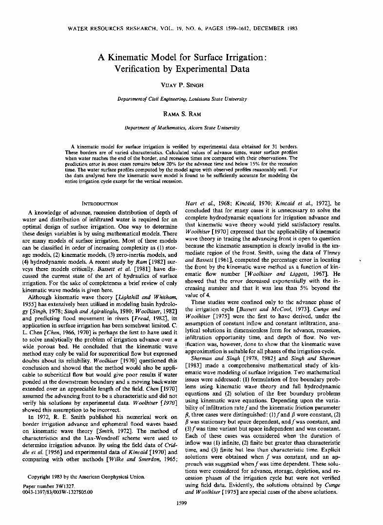
Fig. 1. Solution domain for flow in a freely draining border.

phases, which include advance, storage, and recession. These constitute the irrigation cycle, as shown in Figure 1.

When water is released, there is a front wall of water which advances down the channel. This front wall of water is the

advance front, that is, the moving interface between the water- covered and -uncovered parts of the channel. Let x = s(t) or, inversely, t = •(x) denote the history of this front; this time history is the advance function. This front is a free boundary which has to be determined along with the depth h(x, t) and velocity u(x, t) for a specified ho(t) or q(0, t). The advance phase continues until the water reaches the downstream end of the channel. As shown in the figure, this phase is represented by the domain D•, which is bounded by x = 0, t = •(x), x - L, and t - T; L denotes the length of the field and T the advance time.

Let f(r) be the infiltration rate at time r; the quantity r = t- •(x) denotes the infiltration opportunity time at a point x in the field, that is, the interval of time that water has covered the point x, where t is the total time elapsed since the inflow began. The infiltration rate f(r) is assumed to depend only on the difference r between the total elapsed time and the advance time, that is, it is time dependent but independent of xforx > 0.

If the inflow q(0, t) is continued after water has reached the downstream end of the channel, then the water will continue to accumulate in the channel. This water buildup constitutes the storage phase. As shown in Figure 1, this phase is represented by domain D2, which is bounded by x = 0, T < t < T• and x = L. As soon as the inflow is cut off at t- T•, q(0, t) = 0, t > T•, the storage phase ends and the recession phase begins. The depth of flow at x = 0, t - T• goes to zero instan- taneously. This implies that the kinematic wave assumption does not accommodate vertical recession. As time progresses, the zero depth travels downward. This zero depth is called the drying front. The movement of this drying front characterizes the horizontal recession and continues until all the water is

drained out of the channel. We let t = •(x) denote the time history of the drying front, that is, the moving interface between the part of the channel with h(x, t)= 0 and the part of the channel with h(x, t)> 0. This time history t = •(x), T• < t < T2 is a free boundary whose determination is a part of the solution for the recession phase. This phase is represented by domain D3, which is bounded by x = 0, T• < t < •(x), and

The depth of water h(x, t) and the unknown time history •(x) are subject to the following kinematic wave formulation

SINGH AND RAM: KINEMATIC MODEL FOR SURFACE IRRIGATION 1601

[Sherman and Sinqh, 1978]:

t•h t•

t3•' + •xx (]•h") = - fit - •(x)] h(0, t) = ho(t ) (1)

0<t<T• h(0, t)=0 t>T•

= {fih"-'[x, = 0 (2)

where n e (1, 3] and fi > 0 are kinematic wave parameters.

NUMERICAL SOLUTIONS

Equations (1)-(2) are valid in the solution region comprised of the domains D•, D2, and D 3. The solution to these equations can be found in each of these domains by using the method of characteristics. The characteristic equations of (1) can be written as

dx/dt = nfih n- • (3)

dh/dt = - fit - •(x)] (4)

Sherman and Sinqh [1982] proposed a numerical method to solve (3)-(4) for the entire irrigation cycle. Chen et al. [1981] solved these equations for the advance phase by a simpler method. This study modifies this latter method by making it computationally more efficient for the advance phase and de- velops a semianalytical method for the recession phase. The resulting method is thus part numerical and part analytical.

Domain D a

Central to the solution to be obtained in this domain is the

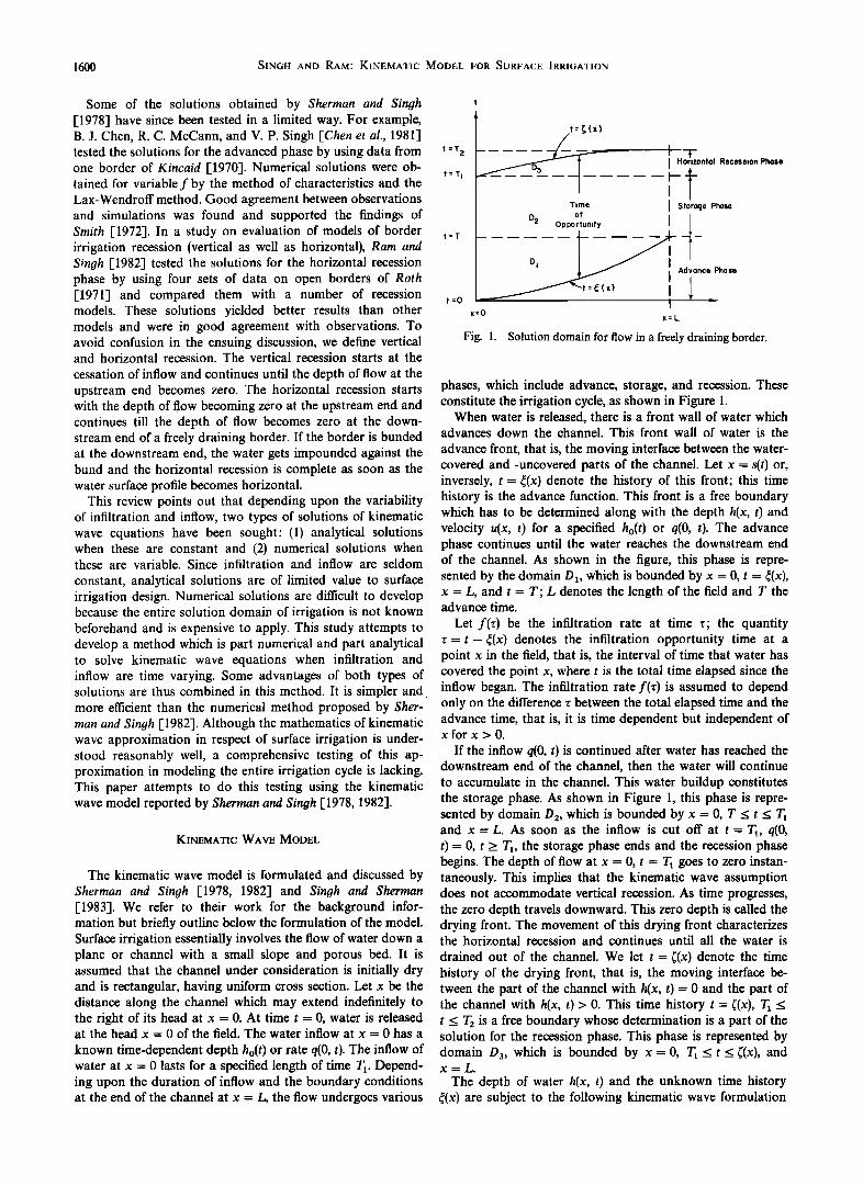
determination of the time history of the advance front, t = •(x). We develop a numerical method, designated as kinematic wave train method (KWT), to solve the initial value problem given by (1)-(2) that yields this time history. We hypothesize that water moves in a series of columns of finite width, as shown in Figure 2a. The front column moves with kinematic velocity. When it moves to a new position, all the following columns move forward, each occupying the place vacated by its immediate predecessor, as shown in Figure 2b. The movement continues until the height of the front column (the depth of the wave front) reduces to a minimum specified by h c, as shown in Figure 2c. Then the preceding column takes

I Water x Column

I 2 3 i-3 i-2

(al x=O

T

Column Water x I ?. 3 i-3 i-2 i-I

x•O

h"G

I W_•ter Column hc • X

I 2 3 i-3 i-2 i-I i

Fig. 2. Movement of water columns.

over the leading column at a given position in x and moves as the wave front. This process continues until the water reaches the end of the border.

To formulate the KWT method, we consider that in (1),/• is constant. For a finite grid spacing Ax and At, (1) can be written as

Ah Ah

A'• + nj•hn-• • = - f(:) (5) Ax

where

Ah = hi+ 1 - h i i _> 1 (6)

where i is a dummy index and assume h = h i. Substituting (6) into (5) and solving for hi+ •,

(Ax)h i + (At)nj•hi n --(Ax At)f(:) hi+ • = Ax + (At) nj•hi n-• (7)

Equation (2), which expresses the inverse of the velocity of kinematic shock, can be used to determine At for a specified grid spacing Ax:

a•i+ 1 -- •i+ 1 -- •i-- axf(•hi n- 1) (8)

where • and •+• are times when wave front reaches xi and x•+ •. Note that (At)i+• -(A•)•+• is dependent upon the position and depth of the front column. Equations (7)-(8) can be solved to yield the advance curve t = •(x) as follows.

1. We assume that the inflow q(0, t) - q0 is constant. The corresponding depth of flow at the upstream end can be calculated using Manning's equation:

G -' (flqo) ø'6 (9)

where G is normal depth of flow at the upstream end. In (9), is expressed as

[} -- rim/So 0'5 (1 O)

where rtm is Manning's roughness coefficient. 2. For a specified Ax and known initial condition h = G at

•i = 0, the advance time •i + • can be calculated using (8). 3. For computing f(:) in (7) it is assumed that it is con-

stant for some time :c, 0 _<: _< :c and follows the Kostyakov equation for: >_ :c:

f (:) = aK: a- • (11)

where K and a are infiltration constants to be determined

empirically; :c can be specified for a particular soil, and (at)•+ • - (a•),+ • = :.

4. The water column at xi was advanced to xi+ • by simultaneously solving (7)-(8) in conjunction with (14).

5. The solution of (7)-(8) was iterated using: = (At)z+ • -A•i+ • until the desired degree of accuracy in hi+ • for a

specified x was obtained. In the present analysis, five iterations were found sufficient to guarantee a precision of the order of 10-5 m.

6. The water column of height h•+ • at xi+ • was permitted to advance to x•+ 2 by (7)-(8). The desired degree of precision in h•+ 2 was obtained by step 5. This process was continued until the height of the front column (depth of the advancing front) reached a specified value hc (Figure 2c). A ratio between the height of the front column (depth of the advancing front) or tip depth (hc) and the normal depth of flow at the upstream end (G) can be used to control the tip depth in the solution. This ratio can be expressed as


For a hydrodynamic model, R t ranges between 0.10 to 0.15 [Kincaid, 1970]. However, in this analysis, R t = 0.05 yielded better results.

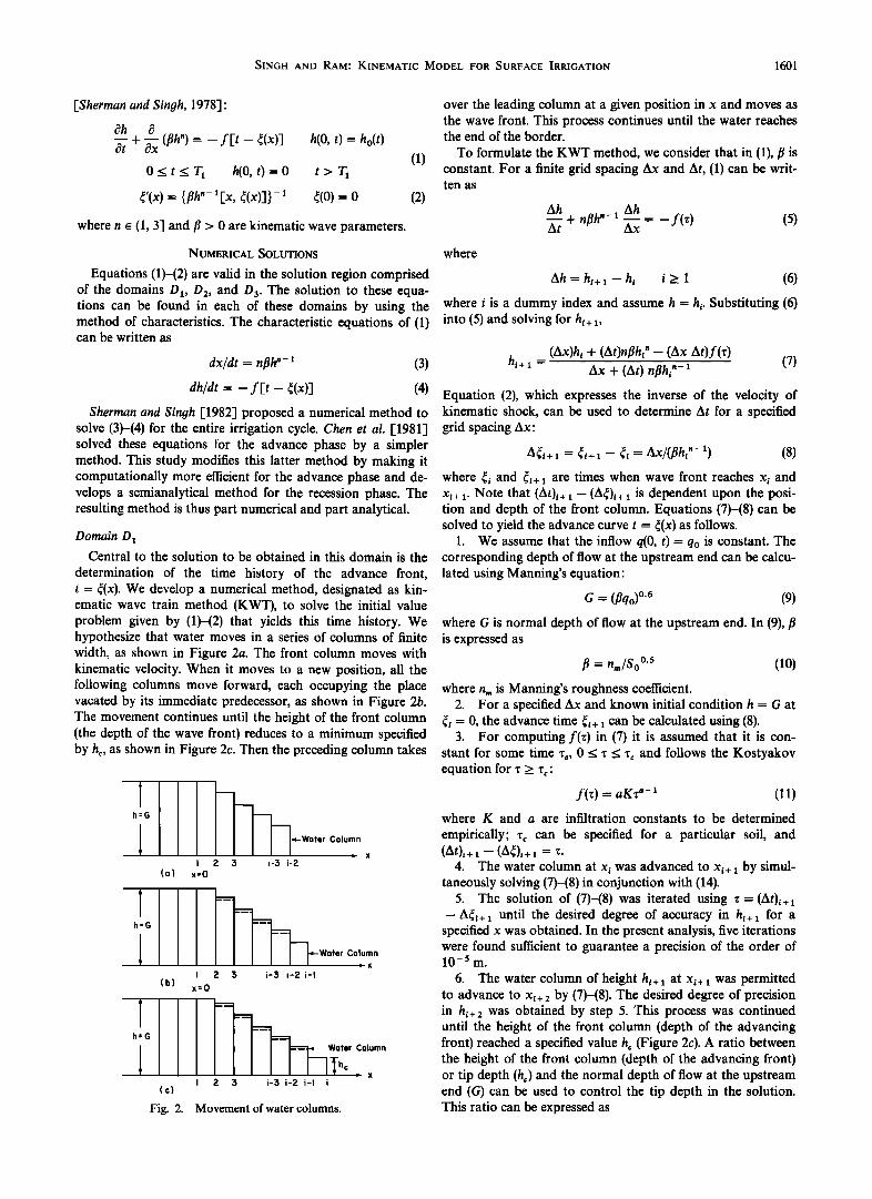
7. Once hc was reached, the water column immediately behind the front was permitted to take over and was allowed to advance. the infiltration opportunity time at any point, when the front was at the position xi. 2, was calculated by •i+ 1 -- •1' •i+ 1 -- •2 ''' •i+ 1 -- •i- 1, •i+ 1 -- •i (Figure 3). Thus we see that for the first column the infiltration opportunity time is always •i+ •- •i = ti+ • subject to its minimum value z c. Similarly, for the second and third columns the infiltration opportunity times are •i+ • - •i- • and •i+ • - •i-2. A similar pattern follows for all preceding columns. The infiltration rate for any column at xi is an average of the rates at xi and xi_ 2. The depth of the first column at xi+ • is hi+ • and is superceded by the second column with depth hi, if hi+ • < hc. Now the second column plays the role of the first column, the third column plays the role of the second column, and so on. This process was continued until water reached the downstream end of the border.

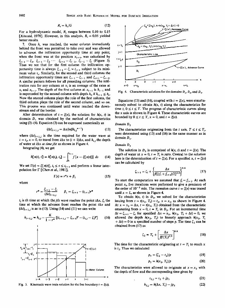
After determination of t = •(x), the solution for h(x, t) in domain D• was obtained by the method of characteristics using (3)-(4). Equation (3) can be expressed numerically as

(At)i+ 1,J = Ax/(n•hijn- 2) (13)

where (At)i+ •,• is the time required for the water wave at t = t•, x = 0, to travel from iAx to (i + 1)Ax, and hiu the depth of water at lax at time jar as shown in Figure 4.

Integrating (4), we get

•i + 1 h[x(t), t] = hl'x(ti), ti] - f{x - •l'x(s)]} ds (14)

We set F(s) = •[x(s)], ti _< s _< ti+• and perform a linear inter- polation for F [Chen et al., 1981],

where

r(s) = r*s + • (15)

r* = •i+l -- •i fi• = •i+ • -- (ti+ •)r* (at) +

ti is th time at which the jth wave reaches the point iAx, •i the time at which the advance front reaches the point iAx and (At)i+ •.• is as in (13). Using (14) and (11) we can write

K

hi+ •.j = h, u 1 - r* [(ti+ •.• - •i+ •)a _ (tiu - •i) a] (16)

'rc +l-ti t:•(x)

ti_l :•i_ I j-I ....

Water Column

i-4 i-$ i-2 i-I i i+l

Fig. 3. Kinematic wave train solution for the free boundary t = •(x).

t=T I

j+l

t: ti, j

f •2: •(x2)' h:h(x2' TI+ At) =0

•t•-t(-x z,•• Characteristic•

j-I -- Advance Curve

• I I I I = X 2 3 i-I i i+l

x=O x:x 2 x:x i x=k

Fig. 4. Characteristic solutions for the domains D•, D 2, and D 3.

Equations (13) and (16), coupled with t = •(x), were simultaneously solved to obtain h(x, t) along the characteristics for time t, 0 _< t < T. The progress of characteristic curves along the x axis is shown in Figure 4. These characteristic curves are bounded by 0 < t _< T, x = 0, and t = •(x).

Domain De

The characteristics originating from the t axis, T < t < T•, were determined using (13) and (16) in the same manner as in domain D2.

Domain D3

The solution in D3 is comprised of h(x, t) and t = •(x). The depth of water at x = 0, t = T• is zero. Central to the solution here is the determination of t = •(x). For a specified x, t = •(x) can be calculated by

+ [(A + To start the computation we assumed that f• =f•+ 2. At each point xi, five iterations were performed to give a precision of the order of 10- 5 min. The recession curve t = •(x) was traced until x = L, as shown in Figure 4.

To obtain h(x, t) in D3, we solved for the characteristics issuing from t = t(x2, r•) = t2, x = x2, as shown in Figure 4. At x = x2 = Ax, t = t(x2, T•) obtained from the characteristic emanating from x = 0, t = T• in D 2. For an incremental time At = •i+ •-•i for specified Ax = x2, h(x2, r• + At)= 0, we allowed the depth h(x2, r•) to linearly approach h(x2, r• + At) = 0 in a specified number of steps p. The time •2 can be obtained from (17) as

FAx ]ø.6 •2: T, + L//f(-•-[)2/sj (18)

The time for the characteristic originating at t = T• to reach x is t 2. Thus we calculated

P, = ((2 - t2)/p (19)

P2 = h(x2, T,)/p (20)

The characteristics were allowed to originate at x = x2 with the depth of flow and the corresponding time given by

ß t2, j = t 2 + jp• (21)

h2,• = h(Ax, T•) - JP2 (22)

$INGH AND RAM' KINEMATIC MODEL FOR SURFACE IRRIGATION 1603

where j = 1, 2, 3,..., p. These characteristics were allowed to progress down the slope by simultaneously solving (13)-(16). These equations can be iterated five times to calculate the depth of flow with an accuracy of the order of 10-5 m. The time of occurrence of zero depth hi+ •,s- 0 is the recession time at xi + •. In this analysis a value of p - 25 was used.

EXPERIMENTAL DATA

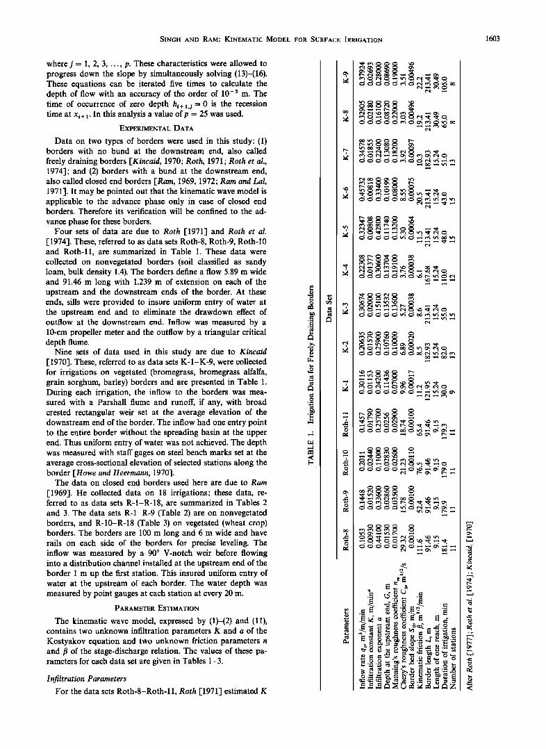
Data on two types of borders were used in this study: (1) borders with no bund at the downstream end, also called freely draining borders ['Kincaid, 1970; Roth, 1971; Roth et al., 19743; and (2) borders with a bund at the downstream end, also called closed end borders ['Ram, 1969, 1972; Ram and Lal, 19713. It may be pointed out that the kinematic wave model is applicable to the advance phase only in case of closed end borders. Therefore its verification will be confined to the ad-

vance phase for these borders. Four sets of data are due to Roth [1971] and Roth et al.

[1974]. These, referred to as data sets Roth-8, Roth-9, Roth-10 and Roth-11, are summarized in Table 1. These data were collected on nonvegetated borders (soil classified as sandy loam, bulk density 1.4). The borders define a flow 5.89 m wide and 91.46 m long with 1.239 m of extension on each of the upstream and the downstream ends of the border. At these ends, sills were provided to insure uniform entry of water at the upstream end and to eliminate the drawdown effect of outflow at the downstream end. Inflow was measured by a 10-cm propeller meter and the outflow by a triangular critical depth flume.

Nine sets of data used in this study are due to Kincaid ['1970]. These, referred to as data sets K-l-K-9, were collected for irrigations on vegetated (bromegrass, bromegrass alfalfa, grain sorghum, barley) borders and are presented in Table 1. During each irrigation, the inflow to the borders was measured with a Parshall flume and runoff, if any, with broad crested rectangular weir set at the average elevation of the downstream end of the border. The inflow had one entry point to the entire border without the spreading basin at the upper end. Thus uniform entry of water was not achieved. The depth was measured with staff gages on steel bench marks set at the average cross-sectional elevation of selected stations along the border [Howe and Heermann, 1970].

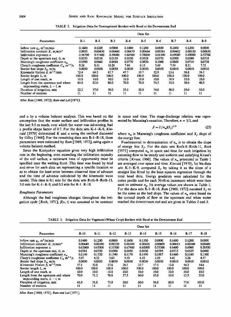
The data on closed end borders used here are due to Ram

[1969-]. He collected data on 18 irrigations; these data, referred to as data sets R-I-R-18, are summarized in Tables 2 and 3. The data sets R-l-R-9 (Table 2) are on nonvegetated borders, and R-10-R-18 (Table 3) on vegetated (wheat crop) borders. The borders are 100 m long and 6 m wide and have rails on each side of the borders for precise leveling. The inflow was measured by a 90 ø V-notch weir before flowing into a distribution channel installed at the upstream end of the border 1 m up the first station. This insured uniform entry of water at the upstream of each border. The water depth was measured by point gauges at each station at every 20 m.

PARAMETER ESTIMATION

The kinematic wave model, expressed by (1)-(2) and (11), contains two unknown infiltration parameters K and a of the Kostyakov equation and two unknown friction parameters n and/• of the stage-discharge relation. The values of these parameters for each data set are given in Tables 1-3.

Infiltration Parameters

For the data sets Roth-8-Roth-11, Roth [1971] estimated K

1604 SINGH AND RAM.' KINEMATIC MODEL FOR SURFACE IRRIGATION

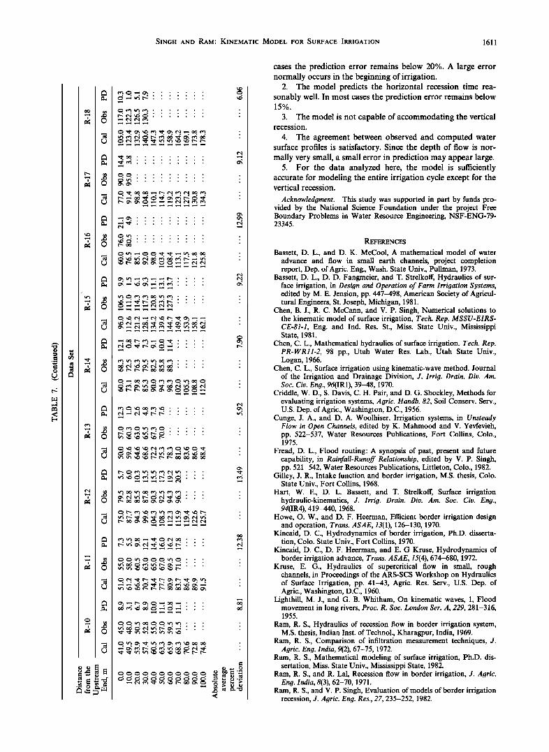
TABLE 2. Irrigation Data for Nonvegetated Borders with Bund at the Downstream End

Data Set

Parameters R- 1 R-2 R-3 R-4 R-5 R-6 R-7 R-8 R-9

Inflow rate qo, m3/m/min Infiltration constant K, m/min a Infiltration exponent a Depth at the upstream end, G, m Manning's roughness coefficient nm Chezy's roughness coefficient C h, m•/2/s Border bed slope So, m/m Kinematic friction//, m x/3/min Border length L, m Length of one reach, m Length from the upstream end where

impounding starts, L - l, m Duration of irrigation, min Number of stations

0.1600 0.1200 0.0800 0.1600 0.1200 0.0800 0.1600 0.0039 0.00450 0.00460 0.00479 0.00464 0.00361 0.00402 0.56700 0.57400 0.59000 0.60500 0.58800 0.61500 0.69000 0.0255 0.0230 0.0150 0.0350 0.0328 0.0370 0.0500 0.0590 0.0660 0.0480 0.0770 0.0920 0.1000 0.0800 9.26 8.11 10.26 7.44 6.15 5.49 7.54 0.0050 0.0050 0.0050 0.0030 0.0030 0.0030 0.0010

72.4 64.5 87.7 47.7 35.7 32.9 23.6 100.0 100.0 100.0 100.0 100.0 100.0 100.0

10.0 10.0 10.0 10.0 10.0 10.0 10.0 80.0 82.0 88.0 70.0 70.0 74.5 35.0

0.1200 0.0800 0.00330 0.00630 0.69000 0.52700 0.0390 0.0310 0.0710 0.0730 8.21 7.72 0.0010 0.0010

26.8 26.2

100.0 100.0 10.0 10.0 38.0 40.5

22.5 37.0 59.0 35.5 50.0 74.0 50.0 59.0 95.0 11 11 11 11 11 11 11 11 11

After Ram [1969, 1972]; Ram and Lal [1971].

and a by a volume balance analysis. This was based on the assumption that the water surface and infiltration profiles in the last 9.5 m reach, over which the water was advancing, had a profile shape factor of 0.7. For the data sets K-l-K-9, Kin- caid [1970] determined K and a using the method discussed by Gilley [1968]. For the remaining data sets R-I-R-18, these parameters were estimated by Ram [1969, 1972], using again a volume balance method.

Since the Kostyakov equation gives very high infiltration rate in the beginning, even exceeding the infiltration capacity of the soil surface, a minimum time of opportunity must be specified near the wetting front. This time was found by trial and error for each data set representing a specific location so as to obtain the least error between observed time of advance

and the time of advance calculated by the kinematic wave model. This time is 0.1 min for the data sets Roth-8-Roth-11, 5.0 min for K-l-K-9, and 0.5 min for R-I-R-18.

Roughness Parameters

Although the bed roughness changes throughout the irrigation cycle [Roth, 1971],/•(x, t) was assumed to be constant

in space and time. The stage-discharge relation was represented by Manning's equation. Therefore, n = 5/3, and

]• = (1/nmXS f) 1/2 (23)

where n m is Manning's roughness coefficient and S t slope of the energy line.

Fundamental to determination of nm is to obtain the slope of energy line S t. For the data sets Roth-8-Roth-11, Roth [1971] computed n m in space and time for each irrigation by assuming flow to be steady and uniform and satisfying Kruse's criteria [Kruse, 1960]. The values of n m presented in Table 1 are averaged over space and time. Kincaid [1970], for his data sets K-l-K-9, computed S t by taking it as the slope of a straight line fitted by the least squares regression through the total head data. Energy gradients were calculated for the entire profile and for each 30.48-m increment which were then used to estimate n m. Its average values are shown in Table 1. For the data sets R-I-R-18, Ram [1969, 1972] assumed S t to be the same as the bed slope. The values of n m were based on the normal depth of flow at the upstream end when water reached the downstream end and are given in Tables 2 and 3.

TABLE 3. Irrigation Data for Vegetated (Wheat Crop) Borders with Bund at the Downstream End

Data Set

Parameters R-10 R-11 R-12 R-13 R-14 R-15 R-16 R-17 R-18

Inflow rate qo, m3/m/min Infiltration constant K, m/min a Infiltration exponent a Depth at the upstream end, G, m Manning's roughness coefficient nm Chezy's roughness coefficient Ch, m•/2/s Border bed slope So, m/m Kinematic friction fi, m x/3/min Border length L, m Length of one reach, m Length from the upstream end where

impounding starts, L - l, m Duration of irrigation, min Number of stations

0.1600 0.1200 0.0800 0.1600 0.1200 0.0800 0.1600 0.1200 0.0800 0.00440 0.00360 0.00530 0.00390 0.00405 0.00609 0.00415 0.00340 0.00460 0.62000 0.63000 0.53300 0.67400 0.60000 0.53300 0.6400 0.6900 0.58500 0.0381 0.0350 0.0300 0.0450 0.0430 0.0395 0.0715 0.0525 0.0440 0.1140 0.1320 0.1540 0.1170 0.1450 0.1887 0.1460 0.1160 0.1300

5.07 4.32 3.63 5.10 4.10 3.10 4.41 5.26 4.57 0.0050 0.0050 0.0050 0.0030 0.0030 0.0030 0.0010 0.0010 0.0010

37.1 32.0 27.6 28.1 22.7 17.5 13.0 16.3 14.6

100.0 100.0 100.0 100.0 100.0 100.0 100.0 100.0 100.0 10.0 10.0 10.0 10.0 10.0 10.0 10.0 10.0 10.0 70.0 71.5 76.0 57.5 60.0 65.0 10.0 15.5 35.0

41.0 51.0 75.0 50.0 60.0 96.0 60.0 77.0 105.0 11 11 11 11 11 11 11 11 11

After Ram [1969, 1972]; Ram and Lal [1971].


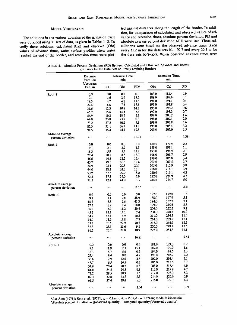
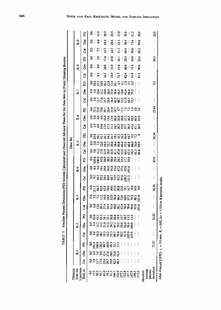
MODEL VERIFICATION

The solutions in the various domains of the irrigation cycle were obtained using 31 sets of data, as given in Tables 1-3. To verify these solutions, calculated (Cal) and observed (Obs) values of advance times, water surface profiles when water reached the end of the border, and recession times were plot-

ted against distances along the length of the border. In addi- tion, for comparison of calculated and observed values of advance and recession times, absolute percent deviation PD and absolute average percent deviation APD were used. These cal- culations were based on the observed advance times taken every 15.2 m for the data sets K-l-K-7 and every .30.5 m for the data sets K-8-K-9. When observed advance times were

TABLE 4. Absolute Percent Deviations (PD) Between Calculated and Observed Advance and Recess- ion Times for the Data Sets on Freely Draining Borders

Roth-8

Distance from the

Upstream End, m

Advance Time, Recession Time, min min

Cal Obs PD* Obs Cal PD

0.0 0.0 0.0 0.0 183.0 181.4 0.9 9.1 1.6 2.0 19.7 188.0 187.8 0.1

18.3 4.7 4.2 11.5 191.0 191.1 0.1 27.4 8.6 7.3 17.6 193.0 193.8 0.4 36.6 12.3 10.8 14.2 195.0 196.2 0.6 45.7 15.6 14.4 8.6 197.0 198.3 0.7 54.9 19.2 18.7 2.6 !98.0 200.2 1.4 64.0 23.8 23.7 0.3 198.0 202.1 2.0 73.2 27.2 30.2 9.9 199.0 203.8 2.6 82.3 31.1 36.2 14.0 199.0 205.4 3.2 91.5 35.4 44.1 19.8 200.0 207.0 3.5

Absolute average percent deviation ......... 10.73 ...... 1.36

Roth-9 0.0 0.0 0.0 0.0 180.5 179.9 0.3 9.1 2.1 2.2 1.9 189.0 191.1 1.1

18.3 5.9 5.2 12.8 193.0 196.9 2.1 27.4 10.1 8.5 18.7 196.0 201.7 2.9 36.6 14.3 12.2 17.4 199.0 205.8 3,4 45.7 19.5 16.3 19.4 202.0 209.5 3.7 54.9 24.4 20.3 20.1 205.0 212.9 3.8 64.0 28.2 24.3 13.1 208.0 216.,1 3.9 73.2 32.3 29.9 8.0 210.0 219.1 4.3 82.3 37.8 35.0 7.9 212.0 221.9 4.7 91.5 42.4 41.0 3.3 214.0 224.7 5.0


Roth-10 0.0 0.0 0.0 0.0 182.0 179.0 1.6 9.1 1.4 2.8 48.9 188.0 197.9 5.3

18.3 3.3 5.6 41.3 194.0 207.7 7.1 27.4 6.9 8.4 18.0 199.0 215.6 8.3 36.6 8.9 11.2 20.4 204.0 222.5 9.1 45.7 13.1 14.1 7.4 208.0 228.7 10.0 54.9 15.1 16.9 10.5 211.0 234.5 11.0 64.0 18.3 19.8 7.8 .214.0 23•.8 12.1 73.2 20.5 22.9 10.7 217.0 244.9 12.9 82.3 23.3 25.6 9.1 220.0 249.7 13.5 91.5 25.7 28.8 10.9 223.0 254.3 14.1


Roth-ll 0.0 0.0 0.0 0.0 181.0 179.3 0.9 9.1 1.9 2.3 15.1 189.0 191.9 1.6

18.3 517 5.6 0.9 194.0 198.5 2.3 27.4 9.4 9.0 4.7 198.0 .203.7 2.0 36.6 12.9 12.6 2.6 202.0 208.4 3.1 45.7 16.5 16.5 0..3 205.0 212.5 3.7 54.9 20.4 20.2 0.8 208.0 216.4 4.0 64.0 24.3 24.3 0.1 210.0 219.9 4.7 73.2 28.5 28.9 1.5 212.0 223.3 5.3 82.3 32.8 33.7 2.5 214.0 226.6 5.9 91.5 37.4 39.4 5.0 216.0 229.7 6.3

,


After Roth [1971]' Roth et al. [1974]' Zc = 0.1 min, R t = 0.05, Ax = 1.524 m' model is kinematic. *Absolute percent deviation = [(observed quantity -computed quantity)/observed quantity].

1606 SINGH AND RAM.' KINEMATIC MODEL FOR SURFACE IRRIGATION

ß

$INGH AND RAM: KINEMATIC MODEL FOR SURFACE IRRIGATION 1607

<

1608 SINGH AND RAM' KINEMATIC MODEL FOR SURFACE IRRIGATION

Observed Data

a, Data Set Roth-9

0 Data Set Roth- 8

240 - Calculated Curve

Advance KWT

------- Recession •- r- •' % •'o o o

•- Roth-9

160

E 120

80

I •, • g• øth-8 I 0 20 40 60 80 I 0 0

DISTANCE, rn

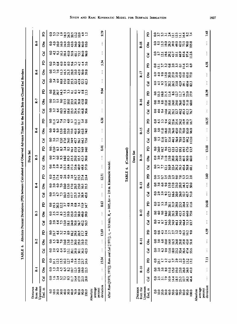
Fig. 5. Advance and recession curves for the data sets Roth-8 and Roth-9.

not available at regular intervals, they were interpolated from figures [Kincaid, 1970]. No data were available on recession time and water surface profile for the data sets K-l-K-7.

Advance

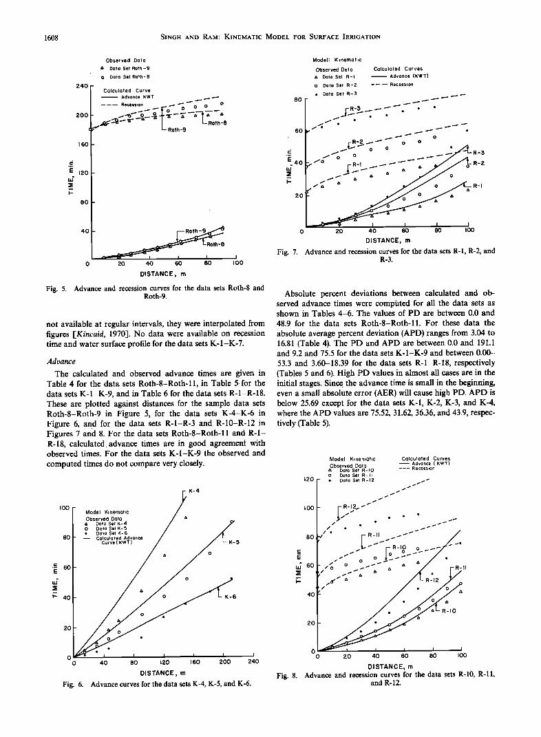
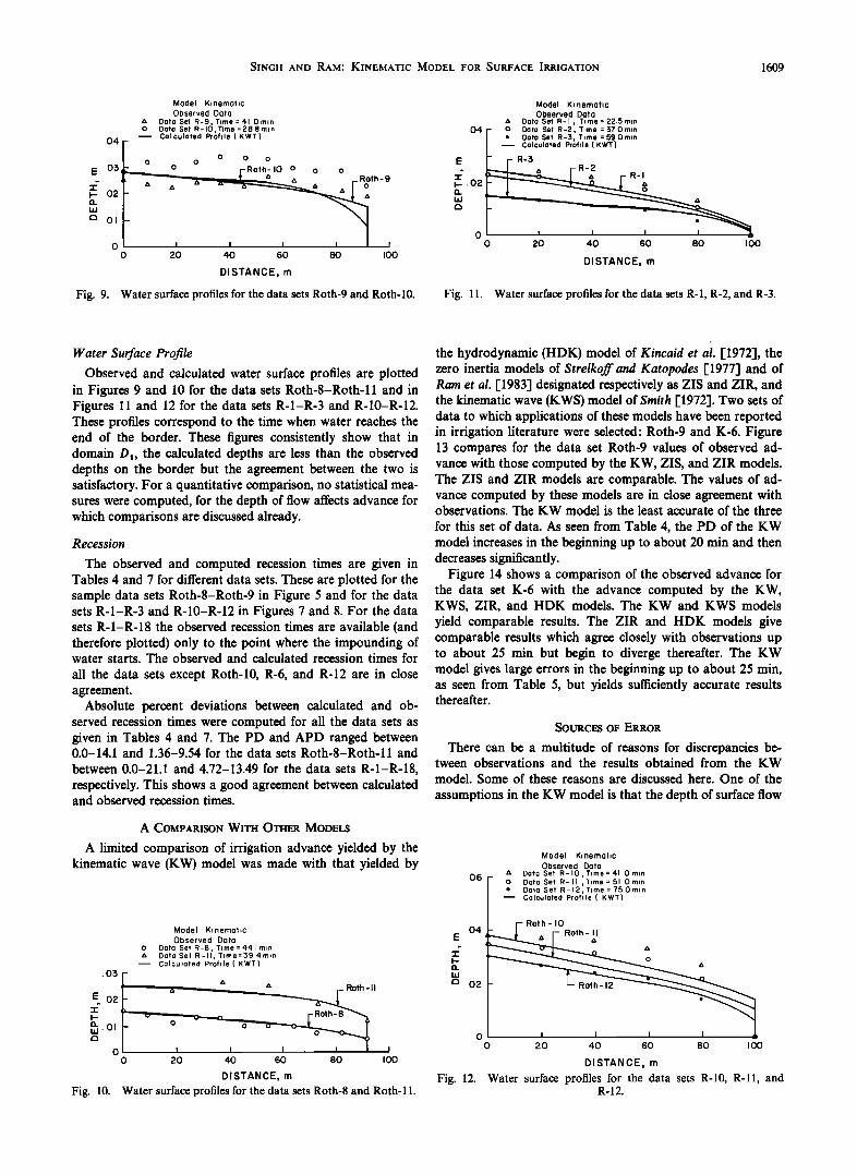
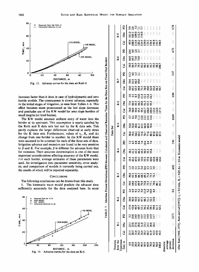
The calculated and observed advance times are given in Table 4 for the data sets Roth-8-Roth-11, in Table 5 for the data sets K-l-K-9, and in Table 6 for the data sets R-I-R-18. These are plotted against distances for the sample data sets Roth-8-Roth-9 in Figure 5, for the data sets K-4-K-6 in Figure 6, and for the data sets R-l-R-3 and R-10-R-12 in Figures 7 and 8. For the data sets Roth-8-Roth-ll and R-I- R-18, calculated, advance times are in good agreement with observed times. For the data sets K-l-K-9 the observed and

computed times do not compare very closely.

Model: K•nemat•c

Observed Data

• Data Set R-

0 Data Set R-

ß Data Set R-3

Calculated Curves

Advance (KWT)

Recession

R-3 •- '• • * j. ß

60 /"•' * '• •' -- '"' •. • o

•R-2 • • o o •• o o

_

I I I I 0 20 40 60 80

DISTANCE, m

Fi•. 7. Advance and recession curves for the data sets E-I, E-•, and E-3.

Absolute percent deviations between calculated and observed advance times were compbted for all the data sets as shown in Tables 4-6. The values of PD are between 0.0 and 48.9 for the data sets Roth-8-Roth-11. For these data the

absolute average percent deviation (APD) ranges from 3.04 to 16.81 (Table 4). The PD and APD are between 0.0 and 191.1 and 9.2 and 75.5 for the data sets K-l-K-9 and between 0.00-

53.3 and 3.60-18.39 for the data sets R-I-R-18, respectively (Tables 5 and 6). High P D values in almost all cases are in the initial stages. Since the advance time is small in the beginning, even a small absolute error (AER) will cause high PD. APD is below 25.69 except for the data sets K-l, K-2, K-3, and K-4, where the APD values are 75.52, 31.62, 36.36, and 43.9, respectively (Table 5).

Model K•nemat•c Calculated Curves • Advance (KWT) Observed Data ---- Recession • Data Set R-IO

o Data Set R-II

120 ß Data Set R-12

r- R_ 12....• "' IOO :- Model K•nemahc / IOO Observed Data / a ß ß ß ... • Data Set K- 4 / I 0 Data Set K- 5

, ß DotoSetK-6 80 r- -- Calculated Advance I Curve (KWT)

A O

40 o K-6

A O 20

O O ß J

0 • 100 0 40 80 120 160 200 240

DISTANCE, rn

DISTANCE, m Fig. 8. Advance and recession curves for the data sets R-10, R-11, Fig. 6. Advance curves for the data sets K-4, K-5, and K-6. and R-12.

SINGH AND RAM' KINEMATIC MODEL FOR SURFACE IRRIGATION 1609

Model K•nemat•c

Observed Data ß • Data Set R-9, T•me -- 41 0 rnln 0 Data Set R-IO,Time =28.Stain

• Calculated Profile (KWT) .04 -

o o o

• • Roth-9 • • • • 0 • .o2

• .01 -

0 20 40 60 80 I00

DISTANCE, m

FiB. •. Watc• surface p•o•]cs fo• the data sets Eoth-9 and Eoth-]O.

Model K• nemat•c Observed Data

ß • Data Set R-I, Time= 22. Stain

.04 I 0 Data Set R-2, T•rne =37.0rain ß Dato Set R-3, Time = 59.0 rmn • Calculated Profile (KWT)

F F .0•

0 ; 0 20 40 60 80 I00

DISTANCE, m

Fig. 11. Water surface profiles for the data sets R-l, R-2, and R-3.

Water Surface Profile

Observed and calculated water surface profiles are plotted in Figures 9 and 10 for the data sets Roth-8-Roth-ll and in Figures 11 and 12 for the data sets R-l-R-3 and R-10-R-12. These profiles correspond to the time when water reaches the end of the border. These figures consistently show that in domain D•, the calculated depths are less than the observed depths on the border but the agreement between the two is satisfactory. For a quantitative comparison, no statistical mea- sures were computed, for the depth of flow affects advance for which comparisons are discussed already.

Recession

The observed and computed recession times are given in Tables 4 and 7 for different data sets. These are plotted for the sample data sets Roth-8-Roth-9 in Figure 5 and for the data sets R-l-R-3 and R-10-R-12 in Figures 7 and 8. For the data sets R-l-R-18 the observed recession times are available (and therefore plotted) only to the point where the impounding of water starts. The observed and calculated recession times for

all the data sets except Roth-10, R-6, and R-12 are in close agreement.

Absolute percent deviations between calculated and observed recession times were computed for all the data sets as given in Tables 4 and 7. The PD and APD ranged between 0.0-14.1 and 1.36-9.54 for the data sets Roth-8-Roth-ll and

between 0.0-21.1 and 4.72-13.49 for the data sets R-I-R-18, respectively. This shows a good agreement between calculated and observed recession times.

A COMPARISON WITH OTHER MODELS

A limited comparison of irrigation advance yielded by the kinematic wave (KW) model was made with that yielded by

Model' K•nemat•c

Observed Data 0 Data Set R-8, TI me = 44 I rn•n ß • Data Set R-II, T•me=39 4rain

• Calculated Profile (KWT)

.03 [ ,, '• '• _ Roth-II E .02

n 01 o Ixl'

0 I I I I 0 20 40 60 80 I00

DISTANCE, m

Fig. 10. Water surface profiles for the data sets Roth-8 and Roth-I l.

the hydrodynamic (HDK) model of Kincaid et ai. [1972], the zero inertia models of Strelkoff and Katopodes [1977] and of Ram et al. [1983] designated respectively as ZIS and ZIR, and the kinematic wave (KWS) model of Smith [1972]. Two sets of data to which applications of these models have been reported in irrigation literature were selected: Roth-9 and K-6. Figure 13 compares for the data set Roth-9 values of observed advance with those computed by the KW, ZIS, and ZIR models. The ZIS and ZIR models are comparable. The values of advance computed by these models are in close agreement with observations. The KW model is the least accurate of the three

for this set of data. As seen from Table 4, the PD of the KW model increases in the beginning up to about 20 min and then decreases significantly.

Figure 14 shows a comparison of the observed advance for the data set K-6 with the advance computed by the KW, KWS, ZIR, and HDK models. The KW and KWS models yield comparable results. The ZIR and HDK models give comparable results which agree closely with observations up to about 25 min but begin to diverge thereafter. The KW model gives large errors in the beginning up to about 25 min, as seen from Table 5, but yields sufficiently accurate results thereafter.

SOURCES OF ERROR

There can be a multitude of reasons for discrepancies between observations and the results obtained from the KW

model. Some of these reasons are discussed here. One of the

assumptions in the KW model is that the depth of surface flow

.O6

.04 E

C3 .02

0 0

Model. K•nemahc

Observed Data '• Data Set R- I0, T•rne: 41 0 rmn

I 0 Data Set R-II ,Time = 510m,n ß Doto Set R-12,T•me = 75.Omen

-- Colculoted Profile (KWT) r- Roth- I0 _

20 40 60 80 I00

DISTANCE, m

Fig. 12. Water surface profiles for the data sets R-10, R-11, and R-12.


8O ß • Observed Doto Set Roth-9

• Colculoted Advonce Curve

6O

.E DEL E

u• 40

2O

0 i i I i 0 20 40 60 80 I00

DISTANCE, rn

Fig. 13. Advance curves for the data set Roth-9.

increases faster than it does in case of hydrodynamic and zero inertia models. The consequence is slower advance, especially in the initial stages of irrigation, as seen from Tables 4-6. This effect becomes more pronounced as the bed slope decreases and precludes use of the KW model for zero slope borders of small lengths (or level basins).

The KW model assumes uniform entry of water into the border at its upstream. This assumption is nearly satisfied by the Roth and R data sets but not by the K data sets. This partly explains the larger differences observed at early times for the K data sets. Furthermore, values of re, Rt, and Ax change from one border to another. In the KW model these were assumed to be constant for each of the three sets of data.

Irrigation advance and recession are found to be very sensitive to/• and K. For example,/• is different for advance from that for recession. Their accurate determination is one of the most

important considerations affecting accuracy of the KW model. For each border, average estimates of these parameters were used. An investigation into parameter sensitivity, error analysis, and comparison of models is currently being carried out, the results of which will be reported separately.

CONCLUSIONS

The following conclusions can be drawn from this study. 1. The kinematic wave model predicts the advance time

sufficiently accurately for the data analyzed here. In most

8O

6O

u• 40

20

ß • Observed Dote Set K- 6 0 KWS MODEL ß ZlR MODEL

• Colculoted Advonce Curve

KW MO•DEL

ß

I i I I

40 80 120 160 200

DISTANCE, rn

Fig. 14. Advance curves for the data set K-6.

I

24O o o. o. o. o. o o o o o o. o '•


cases the prediction error remains below 20%. A large error normally occurs in the beginning of irrigation.

2. The model predicts the horizontal recession time reasonably well. In most cases the prediction error remains below 15%.

3. The model is not capable of accommodating the vertical recession.

4. The agreement between observed and computed water surface profiles is satisfactory. Since the depth of flow is normally very small, a small error in prediction may appear large.

5. For the data analyzed here, the model is sufficiently accurate for modeling the entire irrigation cycle except for the vertical recession.

Acknowledgment. This study was supported in part by funds provided by the National Science Foundation under the project Free Boundary Problems in Water Resource Engineering, NSF-ENG-79- 23345.

REFERENCES

Bassett, D. L., and D. K. McCool, A mathematical model of water advance and flow in small earth channels, project completion report, Dep. of Agric. Eng., Wash. State Univ., Pullman, 1973.

Bassett, D. L., D. D. Fangmeier, and T. Strelkoff, Hydraulics of surface irrigation, in Design and Operation of Farm Irrigation Systems, edited by M. E. Jension, pp. 447-498, American Society of Agricul- tural Engineers, St. Joseph, Michigan, 1981.

Chen, B. J., R. C. McCann, and V. P. Singh, Numerical solutions to the kinematic model of surface irrigation, Tech. Rep. MSSU-EIRS- CE-81-1, Eng. and Ind. Res. St., Miss. State Univ., Mississippi State, 1981.

Chen, C. L., Mathematical hydraulics of surface irrigation. Tech. Rep. PR-WRll-2, 98 pp., Utah Water Res. Lab., Utah State Univ., Logan, 1966.

Chen, C. L., Surface irrigation using kinematic-wave method. Journal of the Irrigation and Drainage Division, J. lrrig. Drain. Div. Am. Soc. Civ. Eng., 96(IR 1), 39-48, 1970.

Criddle, W. D., S. Davis, C. H. Pair, and D. G. Shockley, Methods for evaluating irrigation systems, Agric. Handb. 82, Soil Conserv. Serv., U.S. Dep. of Agric., Washington, D.C., 1956.

Cunge, J. A., and D. A. Woolhiser, Irrigation systems, in Unsteady Flow in Open Channels, edited by K. Mahmood and V. Yevfevieh, pp. 522-537, Water Resources Publications, Fort Collins, Colo., 1975.

Fread, D. L., Flood routing: A synopsis of past, present and future capability, in Rainfall-Runoff Relationship, edited by V. P. Singh, pp. 521-542, Water Resources Publications, Littleton, Colo., 1982.

Gilley, J. R., Intake function and border irrigation, M.S. thesis, Colo. State Univ., Fort Collins, 1968.

Hart, W. E., D. L. Bassett, and T. Strelkoff, Surface irrigation hydraulic-kinematics, J. lrrig. Drain. Div. Am. Soc. Civ. Eng., 94(IR4), 419-440, 1968.

Howe, O. W., and D. F. Heerman, Efficient border irrigation design and operation, Trans. ASAE, 13(1), 126-130, 1970.

Kincaid, D.C., Hydrodynamics of border irrigation, Ph.D. disserta- tion, Colo. State Univ., Fort Collins, 1970.

Kincaid, D.C., D. F. Heerman, and E. G Kruse, Hydrodynamics of border irrigation advance, Trans. ASAE, 15(4), 674-680, 1972.

Kruse, E.G., Hydraulics of supercritical flow in small, rough channels, in Proceedings of the ARS-SCS Workshop on Hydraulics of Surface Irrigation, pp. 41-43, Agric. Res. Serv., U.S. Dep. of Agric., Washington, D.C., 1960.

Lighthill, M. J., and G. B. Whitham, On kinematic waves, 1, Flood movement in long rivers, Proc. R. Soc. London Set. A, 229, 281-316, 1955.

Ram, R. S., Hydraulics of recession flow in border irrigation system, M.S. thesis, Indian Inst. of Technol., Kharagpur, India, 1969.

Ram, R. S., Comparison of infiltration measurement techniques, J. Agric. Eng. India, 9(2), 67-75, 1972.

Ram, R. S., Mathematical modeling of surface irrigation, Ph.D. dis- sertation, Miss. State Univ., Mississippi State, 1982.

Ram, R. S., and R. Lal, Recession flow in border irrigation, J. Agric. Eng. India, 8(3), 62-70, 1971.

Ram, R. S., and V. P. Singh, Evaluation of models of border irrigation recession, J. Agric. Eng. Res., 27, 235-252, 1982.


Ram, R. S., V. P. Singh, and S. N. Prasad, Mathematical modeling of border irrigation, Water Resour. Rep. 5, Dep. of Civ. Eng., La. State Univ., Baton Rouge, 1983.

Roth, R. L., Roughness during border irrigation, M.S. thesis, Univ. of Ariz., Tucson, 1971.

Roth, R. L., D. W. Fonken, D. D. Fangmeier, and K. T. Atchison, Data for border irrigation models, Trans. ASAE, 8, 157-161, 1974.

Sherman, B., and V. P. Singh, A kinematic model for surface irrigation, Water Resour. Res., 14(2), 357-364, 1978.

Sherman, B., and V. P. Singh, A kinematic model for surface irrigation: An extension, Water Resour. Res.i •8(3), 659-667, 1982.

Singh, V. P., Mathematical modeling of watershed runoff, paper presented at the International Conference on Water Resources Engi- neering, Int. Assoc. for Hydraul. Res., Bangkok, Thailand, 1978.

Singh, V. P., and N. Agiralioglu, A mathematical study of diverging flow, 1, Analytical solutions, Tech. Rep. MSSU-EIRS-CE-80-3, 175 pp., Eng. and Ind. Res. St., Miss. State Univ., Mississippi State, 1980.

Singh, V. P., and B. Sherman, A kinematic study of surface irrigation: Mathematical solutions, Tech. Rep. WRR4, Water Resour. Pro- gram, Dep. of Civ. Eng., La. State Univ., Baton Rouge, 1983.

Smith, R. E., Border irrigation advance and ephemeral flood waves, J. Irrig. Drain. Div. Am. Soc. Civ. Eng., 98(IR2), 289-307, 1972.

Strelkoff, T., and N. T. Katopodes, Border irrigation hydraulics with

zero inertia, J. Irrig. Drain. Div. Am. Soc. Civ. Eng., 103(IR3), 325- 342, 1977.

Tinney, E. R., and D. L. Bassett, Terminal shape of a shallow liquid front, J. Hydraul. Div. Am. Soc. Civ. Eng., 87(HY5), 117-133, 1961.

Wilke, O., and E. T. Smerdon, A solution of the irrigation advance problem, J. Irrig. Drain. Div. Am. Soc. Civ. Eng., 91(IR3), 23-34, 1965.

Woolhiser, D. A., Discussion of "Surface irrigation using kinematic- wave method by C. L. Chen," J. Irrig. Drain. Div. Am. Soc. Civ. Eng., 96(IR4), 498-500, 1970.

Woolhiser, D. A., Physically based models of watershed runoff, in Rainfall-Runoff Relationship, edited by V. P. Singh, pp. 189-202, Water Resources Publications, Littleton, Colo., 1982.

Woolhiser, D. A., and J. A. Liggett, Unsteady, one-dimensional flow over a plane: The rising hydrograph, Water Resour. Res., 3(3), 753- 771, 1967.

R. S. Ram, Department of Mathematics, Alcorn State University, Lorman, MS 39096.

V. P. Singh, Department of Civil Engineering, Louisiana State Uni- versity, Baton Rouge, LA 70803.

(Received October 29, 1982; revised July 21, 1983;

accepted August 4, 1983.)

a kinematic model for surface irrigation - oaktrust

Documents