EURASIP Journal on Applied Signal Processing 2004:7, 1021–1035c© 2004 Hindawi Publishing Corporation

A Hybrid Resynthesis Model for Hammer-StringInteraction of Piano Tones

Julien BensaLaboratoire de Mecanique et d’Acoustique, Centre National de la Recherche Scientifique (LMA-CNRS),13402 Marseille Cedex 20, FranceEmail: bensa@lma.cnrs-mrs.fr

Kristoffer JensenDatalogisk Institut, Københavns Universitet, Universitetsparken 1, 2100 København, DenmarkEmail: krist@diku.dk

Richard Kronland-MartinetLaboratoire de Mecanique et d’Acoustique, Centre National de la Recherche Scientifique (LMA-CNRS),13402 Marseille Cedex 20, FranceEmail: kronland@lma.cnrs-mrs.fr

Received 7 July 2003; Revised 9 December 2003

This paper presents a source/resonator model of hammer-string interaction that produces realistic piano sound. The source isgenerated using a subtractive signal model. Digital waveguides are used to simulate the propagation of waves in the resonator.This hybrid model allows resynthesis of the vibration measured on an experimental setup. In particular, the nonlinear behaviorof the hammer-string interaction is taken into account in the source model and is well reproduced. The behavior of the modelparameters (the resonant part and the excitation part) is studied with respect to the velocities and the notes played. This modelexhibits physically and perceptually related parameters, allowing easy control of the sound produced. This research is an essentialstep in the design of a complete piano model.

Keywords and phrases: piano, hammer-string interaction, source-resonator model, analysis/synthesis.

1. INTRODUCTION

This paper is a contribution to the design of a com-plete piano-synthesis model. (Sound examples obtained us-ing the method described in this paper can be foundat www.lma.cnrs-mrs.fr/∼kronland/JASP/sounds.html.) It isthe result of several attempts [1, 2], eventually leading to astable and robust methodology. We address here the model-ing for synthesis of a key aspect of piano tones: the hammer-string interaction. This model will ultimately need to belinked to a soundboard model to accurately simulate pianosounds.

The design of a synthesis model is strongly linked to thespecificity of the sounds to be produced and to the expecteduse of the model. This work was done in the frameworkof the analysis-synthesis of musical sounds; we seek bothreconstructing a given piano sound and using the synthe-sis model in a musical context. The perfect reconstructionof given sounds is a strong constraint: the synthesis modelmust be designed so that the parameters can be extracted

from the analysis of natural sounds. In addition, the playingof the synthesis model requires a good relationship betweenthe physics of the instrument, the synthesis parameters, andthe generated sounds. This relationship is crucial to havinga good interaction between the “digital instrument” and theplayer, and it will constitute the most important aspects ourpiano model has to deal with.

Music based on the so-called “sound objects”—likeelectro-acoustic music or “musique concrete”—lies on syn-thesis models allowing subtle and natural transformationsof the sounds. The notion of natural transformation ofsounds consists here in transforming them so that they cor-respond to a physical modification of the instrument. Asa consequence, such sound transformations calls for themodel to include physical descriptions of the instrument.Nevertheless, the physics of musical instruments is some-times too complicated to be exhaustively taken into ac-count, or not modeled well enough to lead to satisfactorysounds. This is the case of the piano, for which hundredsof mechanical components are connected [3], and for which

1022 EURASIP Journal on Applied Signal Processing

the hammer-string interaction still poses physical modelingproblems.

To take into account the necessary simplifications madein the physical description of the piano sounds, we have usedhybrid models that are obtained by combining physical andsignal synthesis models [4, 5]. The physical model simulatesthe physical behavior of the instrument whereas the signalmodel seeks to recreate the perceptual effect produced by theinstrument. The hybrid model provides a perceptually plau-sible resynthesis of a sound as well as intimate manipulationsin a physically and perceptually relevant way. Here, we haveused a physical model to simulate the linear string vibration,and a physically informed signal model to simulate the non-linear interaction between the string and the hammer.

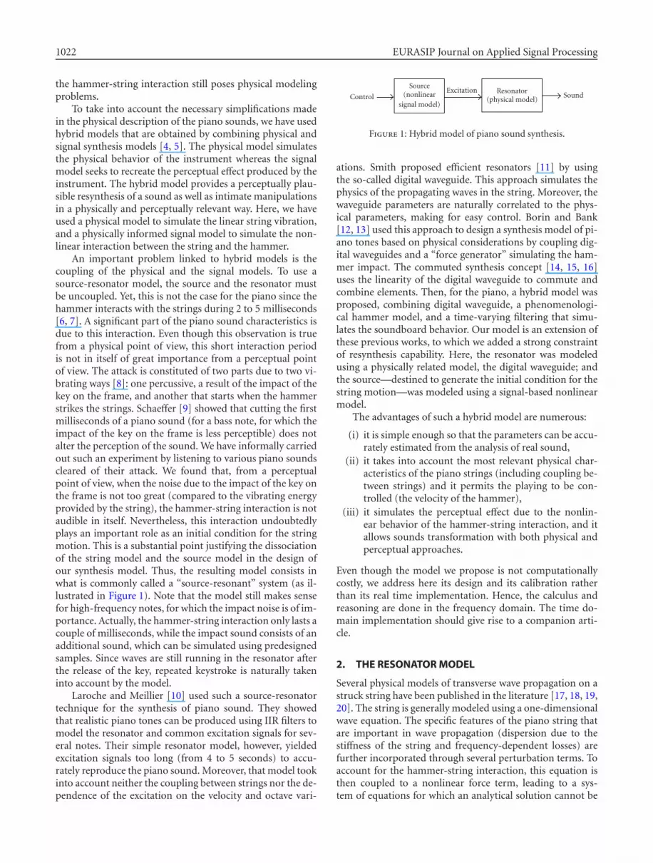
An important problem linked to hybrid models is thecoupling of the physical and the signal models. To use asource-resonator model, the source and the resonator mustbe uncoupled. Yet, this is not the case for the piano since thehammer interacts with the strings during 2 to 5 milliseconds[6, 7]. A significant part of the piano sound characteristics isdue to this interaction. Even though this observation is truefrom a physical point of view, this short interaction periodis not in itself of great importance from a perceptual pointof view. The attack is constituted of two parts due to two vi-brating ways [8]: one percussive, a result of the impact of thekey on the frame, and another that starts when the hammerstrikes the strings. Schaeffer [9] showed that cutting the firstmilliseconds of a piano sound (for a bass note, for which theimpact of the key on the frame is less perceptible) does notalter the perception of the sound. We have informally carriedout such an experiment by listening to various piano soundscleared of their attack. We found that, from a perceptualpoint of view, when the noise due to the impact of the key onthe frame is not too great (compared to the vibrating energyprovided by the string), the hammer-string interaction is notaudible in itself. Nevertheless, this interaction undoubtedlyplays an important role as an initial condition for the stringmotion. This is a substantial point justifying the dissociationof the string model and the source model in the design ofour synthesis model. Thus, the resulting model consists inwhat is commonly called a “source-resonant” system (as il-lustrated in Figure 1). Note that the model still makes sensefor high-frequency notes, for which the impact noise is of im-portance. Actually, the hammer-string interaction only lasts acouple of milliseconds, while the impact sound consists of anadditional sound, which can be simulated using predesignedsamples. Since waves are still running in the resonator afterthe release of the key, repeated keystroke is naturally takeninto account by the model.

Laroche and Meillier [10] used such a source-resonatortechnique for the synthesis of piano sound. They showedthat realistic piano tones can be produced using IIR filters tomodel the resonator and common excitation signals for sev-eral notes. Their simple resonator model, however, yieldedexcitation signals too long (from 4 to 5 seconds) to accu-rately reproduce the piano sound. Moreover, that model tookinto account neither the coupling between strings nor the de-pendence of the excitation on the velocity and octave vari-

Control

Source(nonlinear

signal model)

Excitation Resonator(physical model)

Sound

Figure 1: Hybrid model of piano sound synthesis.

ations. Smith proposed efficient resonators [11] by usingthe so-called digital waveguide. This approach simulates thephysics of the propagating waves in the string. Moreover, thewaveguide parameters are naturally correlated to the phys-ical parameters, making for easy control. Borin and Bank[12, 13] used this approach to design a synthesis model of pi-ano tones based on physical considerations by coupling dig-ital waveguides and a “force generator” simulating the ham-mer impact. The commuted synthesis concept [14, 15, 16]uses the linearity of the digital waveguide to commute andcombine elements. Then, for the piano, a hybrid model wasproposed, combining digital waveguide, a phenomenologi-cal hammer model, and a time-varying filtering that simu-lates the soundboard behavior. Our model is an extension ofthese previous works, to which we added a strong constraintof resynthesis capability. Here, the resonator was modeledusing a physically related model, the digital waveguide; andthe source—destined to generate the initial condition for thestring motion—was modeled using a signal-based nonlinearmodel.

The advantages of such a hybrid model are numerous:

(i) it is simple enough so that the parameters can be accu-rately estimated from the analysis of real sound,

(ii) it takes into account the most relevant physical char-acteristics of the piano strings (including coupling be-tween strings) and it permits the playing to be con-trolled (the velocity of the hammer),

(iii) it simulates the perceptual effect due to the nonlin-ear behavior of the hammer-string interaction, and itallows sounds transformation with both physical andperceptual approaches.

Even though the model we propose is not computationallycostly, we address here its design and its calibration ratherthan its real time implementation. Hence, the calculus andreasoning are done in the frequency domain. The time do-main implementation should give rise to a companion arti-cle.

2. THE RESONATOR MODEL

Several physical models of transverse wave propagation on astruck string have been published in the literature [17, 18, 19,20]. The string is generally modeled using a one-dimensionalwave equation. The specific features of the piano string thatare important in wave propagation (dispersion due to thestiffness of the string and frequency-dependent losses) arefurther incorporated through several perturbation terms. Toaccount for the hammer-string interaction, this equation isthen coupled to a nonlinear force term, leading to a sys-tem of equations for which an analytical solution cannot be

Hybrid Resynthesis of Piano Tones 1023

exhibited. Since the string vibration is transmitted only tothe radiating soundboard at the bridge level, it is not use-ful to numerically calculate the entire spatial motion of thestring. The digital waveguide technique [11] provides an ef-ficient way of simulating the vibration at the bridge level ofthe string, when struck at a given location by the hammer.Moreover, the parameters of such a model can be estimatedfrom the analysis of real sounds [21].

2.1. The physics of vibrating strings

We present here the main features of the physical modeling ofpiano strings. Consider the propagation of transverse wavesin a stiff damped string governed by the motion equation[21]

∂2y

∂t2− c2 ∂

2y

∂x2+ κ2 ∂

4y

∂x4+ 2b1

∂y

∂t− 2b2

∂3y

∂x2∂t= P(x, t), (1)

where y is the transverse displacement, c the wave speed,κ the stiffness coefficient, b1 and b2 the loss parameters.Frequency-dependent loss is introduced via mixed time-space derivative terms (see [21, 22] for more details). We ap-ply fixed boundary conditions

y|x=0 = y|x=L = ∂2y

∂x2

∣∣∣∣x=0

= ∂2y

∂x2

∣∣∣∣x=L

= 0, (2)

where L is the length of the string. After the hammer-stringcontact, the force P is equal to zero and this system can besolved. An analytical solution can be expressed as a sum ofexponentially damped sinusoids:

y(x, t) =∞∑n=1

an(x)e−αnteiωnt, (3)

where an is the amplitude, αn is the damping coefficient, andωn is the frequency of the nth partial. Due to the stiffness, thewaves are dispersed and the partial frequencies, which are notperfectly harmonic, are given by [23]

ωn = 2πnω0

√1 + Bn2, (4)

where ω0 is the fundamental radial frequency of the stringwithout stiffness, and B is the inharmonicity coefficient [23].The losses are frequency dependent and expressed by [21]

αn = −b1 − b2

π2

2BL2

− 1 +

√√√√1 + 4B(ωn

ω0

)2. (5)

The spectral content of the piano sound, and of most mu-sical instruments, is modified with respect to the dynamics.For the piano, this nonlinear behavior consists of an increaseof the brightness of the sound and it is linked mainly to thehammer-string contact (the nonlinear nature of the gener-ation of longitudinal waves also participates in the increaseof brightness; we do not take this phenomena into accountsince we are interested only in transversal waves). The stiff-

E(ω) D(ω) F(ω) S(ω)

G(ω)

Figure 2: Elementary digital waveguide (named G).

ness of the hammer felt increases with the impact velocity. Inthe next paragraph, we show how the waveguide model pa-rameters are related to the amplitudes, damping coefficients,and frequencies of each partial.

2.2. Digital waveguide modeling

2.2.1. The single string case: elementary digitalwaveguide

To model wave propagation in a piano string, we use a digitalwaveguide model [11]. In the single string case, the elemen-tary digital waveguide model (named G) we used consists ofa single loop system (Figure 2) including

(i) a delay line (a pure delay filter named D) simulatingthe time the waves take to travel back and forth in themedium,

(ii) a filter (named F) taking into account the dissipationand dispersion phenomena, together with the bound-ary conditions. The modulus of F is then related to thedamping of the partials and the phase to inharmonic-ity in the string,

(iii) an input E corresponding to the frequency-dependentenergy transferred to the string by the hammer,

(iv) an output S representing the vibrating signal measuredat an extremity of the string (at the bridge level).

The output of the digital waveguide driven by a deltafunction can be expanded as a sum of exponentially dampedsinusoids. The output thus coincides with the solution of themotion equation of transverse waves in a stiff damped stringfor a source term given by a delta function force. As shown in[21, 24], the modulus and phase of F are related to the damp-ing and the frequencies of the partials by the expressions

∣∣F(ωn)∣∣ = eαnD,

arg(F(ωn)) = ωnD − 2nπ,

(6)

with ωn and αn given by (4) and (5).After some calculations (see [21]), we obtain the expres-

sions of the modulus and the phase of the loop filter in termsof the physical parameters:

∣∣F(ω)∣∣ � exp

(−D

[b1 +

b2π2ξ

2BL2

]), (7)

arg(F(ω)

) � Dω−Dω0

√ξ

2B, (8)

1024 EURASIP Journal on Applied Signal Processing

with

ξ = −1 +

√1 +

4Bω2

ω20

(9)

in terms of the inharmonicity coefficient B [23].

2.2.2. The multiple strings case: coupled digitalwaveguides

In the middle and the treble range of the piano, there aretwo or three strings for each note in order to increase the ef-ficiency of the energy transmission towards the bridge. Thevibration produced by this coupled system is not the super-position of the vibrations produced by each string. It is theresult of a complex coupling between the modes of vibra-tion of these strings [25]. This coupling leads to phenomenalike beats and double decays on the amplitude of the par-tials, which constitute one of the most important features ofthe piano sound. Beats are used by professionals to preciselytune the doublets or triplets of strings. To resynthesize the vi-bration of several strings at the bridge level, we use coupleddigital waveguides. Smith [14] proposed a coupling modelwith two elementary waveguides. He assumed that the twostrings were coupled to the same termination, and that thelosses were lumped to the bridge impedance. This techniqueleads to a simple model necessitating only one loss filter. Butthe decay times and the coupling of the modes are not in-dependent. Valimaki et al. [26] proposed another approachthat couples two digital waveguides through real gain ampli-fiers. In that case, the coupling is the same for each partial,and the time behavior of the partials is similar. For synthesispurpose, Bank [27] showed that perceptually plausible beat-ing sound can be obtained by adding only a few resonatorsin parallel.

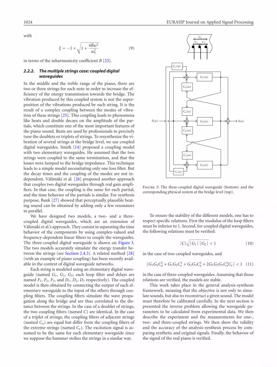
We have designed two models, a two- and a three-coupled digital waveguides, which are an extension ofValimaki et al.’s approach. They consist in separating the timebehavior of the components by using complex-valued andfrequency-dependent linear filters to couple the waveguides.The three-coupled digital waveguide is shown on Figure 3.The two models accurately simulate the energy transfer be-tween the strings (see Section 2.4.3). A related method [28](with an example of piano coupling) has been recently avail-able in the context of digital waveguide networks.

Each string is modeled using an elementary digital wave-guide (named G1, G2, G3; each loop filter and delays arenamed F1, F2, F3, and D1, D2, D3 respectively). The coupledmodel is then obtained by connecting the output of each el-ementary waveguide to the input of the others through cou-pling filters. The coupling filters simulate the wave propa-gation along the bridge and are thus correlated to the dis-tance between the strings. In the case of a doublet of strings,the two coupling filters (named C) are identical. In the caseof a triplet of strings, the coupling filters of adjacent strings(named Ca) are equal but differ from the coupling filters ofthe extreme strings (named Ce). The excitation signal is as-sumed to be the same for each elementary waveguide sincewe suppose the hammer strikes the strings in a similar way.

Ce

Ca Ca

E(ω)

Ce(ω)

Ce(ω)

Ca(ω)

Ca(ω)

Ca(ω)

Ca(ω)

G1(ω)

G2(ω)

G3(ω)

S(ω)

Figure 3: The three-coupled digital waveguide (bottom) and thecorresponding physical system at the bridge level (top).

To ensure the stability of the different models, one has torespect specific relations. First the modulus of the loop filtersmust be inferior to 1. Second, for coupled digital waveguides,the following relations must be verified:

|C|√∣∣G1

∣∣∣∣G2∣∣ < 1 (10)

in the case of two-coupled waveguides, and

∣∣G1G2C2a + G1G3C

2e + G2G3C

2a + 2G1G2G3C

2aCe

∣∣ < 1 (11)

in the case of three-coupled waveguides. Assuming that thoserelations are verified, the models are stable.

This work takes place in the general analysis-synthesisframework, meaning that the objective is not only to simu-late sounds, but also to reconstruct a given sound. The modelmust therefore be calibrated carefully. In the next section ispresented the inverse problem allowing the waveguide pa-rameters to be calculated from experimental data. We thendescribe the experiment and the measurements for one-,two- and three-coupled strings. We then show the validityand the accuracy of the analysis-synthesis process by com-paring synthetic and original signals. Finally, the behavior ofthe signal of the real piano is verified.

Hybrid Resynthesis of Piano Tones 1025

2.3. The inverse problem

We address here the estimation of the parameters of each el-ementary waveguide as well as the coupling filters from theanalysis of a single signal (measured at the bridge level). Forthis, we assume that in the case of three-coupled strings thesignal is composed of a sum of three exponentially decay-ing sinusoids for each partial (and respectively one and twoexponentially decaying sinusoids in the case of one and twostrings). The estimation method is a generalization of the onedescribed in [29] for one and two strings. It can be summa-rized as follows: start by isolating each triplet of the measuredsignal through bandpass filtering (a truncated Gaussian win-dow); then use the Hilbert transform to get the correspond-ing analytic signal and obtain the average frequency of thecomponent by derivating the phase of this analytic signal; fi-nally, extract from each triplet the three amplitudes, dampingcoefficients, and frequencies of each partial by a parametricmethod (Steiglitz-McBride method [30]).

The second part of the process is described in detail in theappendix. In brief, we identify the Fourier transform of thesum of the three exponentially damped sinusoids (the mea-sured signal) with the transfer function of the digital wave-guide (the model output). This identification leads to a lin-ear system that admits an analytical solution in the case ofone or two strings. In the case of three coupled strings, thesolution can be found only numerically. The process gives anestimation of the modulus and of the phase of each filter nearthe resonance peaks as a function of the amplitudes, damp-ing coefficients, and frequencies. Once the resonator modelis known, we extract the excitation signal by a deconvolutionprocess with respect to the waveguide transfer function. Sincethe transfer function has been identified near the resonantpeaks, the excitation is also estimated at discrete frequencyvalues corresponding to the partial frequencies. This excita-tion corresponds to the signal that has to be injected into theresonator to resynthesize the actual sound.

2.4. Analysis of experimental data and validationof the resonator model

We describe here first an experimental setup allowing themeasurement of the vibration of one, two, or three stringsstruck by a hammer for different velocities. Then we showhow to estimate the resonator parameters from those mea-surements, and finally, we compare original and synthesizedsignals. This experimental setup is an essential step that vali-dates the estimation method. Actually, estimating the param-eters of one-, two-, or three-coupled digital waveguides fromonly one signal is not a trivial process. Moreover, in a real pi-ano, many physical phenomena are not taken into account inthe model presented in the previous section. It is then neces-sary to verify the validity of the model on a laboratory exper-iment before applying the method to the piano case.

2.4.1. Experimental setup

On the top of a massive concrete support, we have attacheda piece of a bridge taken from a real piano. On the otherextremity of the structure, we have attached an agraffe on

0.7

0.8

0.9

1

1.1

4

3

21 1000

20003000Velocity (m/s)

Frequency (Hz)

Modulus

Figure 4: Amplitude of filter F as a function of the frequency andof hammer velocity.

a hardwood support. The strings are tightened between thebridge and the agraffe and tuned manually. It is clear thatthe strings are not totally uncoupled to their support. Nev-ertheless, this experiment has been used to record signalsof struck strings, in order to validate the synthesis models,and was it entirely satisfactory for this purpose. One, two, orthree strings are struck with a hammer linked to an electron-ically piloted key. By imposing different voltages to the sys-tem, one can control the hammer velocity in a reproducibleway. The precise velocity is measured immediately after es-capement by using an optic sensor (MTI 2000, probe module2125H) pointing to the side of the head of the hammer. Thevibration at the bridge level is measured by an accelerome-ter (B&K 4374). The signals are directly recorded on digitalaudio tape. Acceleration signals correspond to hammer ve-locities between 0.8 m.s−1 and 5.7 m.s−1.

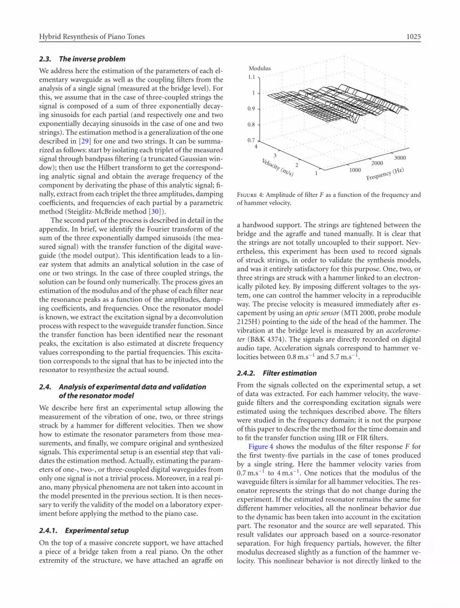
2.4.2. Filter estimation

From the signals collected on the experimental setup, a setof data was extracted. For each hammer velocity, the wave-guide filters and the corresponding excitation signals wereestimated using the techniques described above. The filterswere studied in the frequency domain; it is not the purposeof this paper to describe the method for the time domain andto fit the transfer function using IIR or FIR filters.

Figure 4 shows the modulus of the filter response F forthe first twenty-five partials in the case of tones producedby a single string. Here the hammer velocity varies from0.7 m.s−1 to 4 m.s−1. One notices that the modulus of thewaveguide filters is similar for all hammer velocities. The res-onator represents the strings that do not change during theexperiment. If the estimated resonator remains the same fordifferent hammer velocities, all the nonlinear behavior dueto the dynamic has been taken into account in the excitationpart. The resonator and the source are well separated. Thisresult validates our approach based on a source-resonatorseparation. For high frequency partials, however, the filtermodulus decreased slightly as a function of the hammer ve-locity. This nonlinear behavior is not directly linked to the

1026 EURASIP Journal on Applied Signal Processing

0.7

0.8

0.9

1

1.1

4

3

21 1000

20003000Velocity (m/s)

Frequency (Hz)

Modulus

Figure 5: Amplitude of filter F2 (three-coupled waveguide model)as a function of the frequency and of hammer velocity.

hammer-string contact. It is mainly due to nonlinear phe-nomena involved in the wave propagation. At large ampli-tude motion, the tension modulation introduces greater in-ternal losses (this effect is even more pronounced in pluckedstrings than in struck strings).

The filter modulus slowly decreases (as a function of fre-quency) from a value close to 1. Since the higher partials aremore damped than the lower ones, the amplitude of the filterdecreases as the frequency increases. The value of the filtermodulus (close to 1) suggests that the losses are weak. Thisis true for the piano string and is even more obvious on thisexperimental setup, since the lack of a soundboard limits theacoustic field radiation. More losses are expected in the realpiano.

We now consider the multiple strings case. From a phys-ical point of view, the behavior of the filters F1, F2, and F3

(which characterize the intrinsic losses) of the coupled digi-tal waveguides should be similar to the behavior of the filterF for a single string, since the strings are supposed identical.This is verified except for high-frequency partials. This be-havior is shown on Figure 5 for filter F2 of the three-coupledwaveguide model. Some artifacts pollute the drawing at highfrequencies. The poor signal/noise ratio at high frequency(above 2000 Hz) and low velocity introduce error terms inthe analysis process, leading to mistakes on the amplitudes ofthe loop filters (for instance, a very small value of the modu-lus of one loop filter may be compensated by a value greaterthan one for another loop filter; the stability of the coupledwaveguide is then preserved). Nevertheless, this does not al-ter the synthetic sound since the corresponding partials (highfrequency) are weak and of short duration.

The phase is also of great importance since it is relatedto the group delay of the signal and consequently directlylinked to the frequency of the partials. The phase is a non-linear function of the frequency (see (8)). It is constant withthe hammer velocity (see Figure 6) since the frequencies ofthe partials are always the same (linearity of the wave propa-gation).

0

2

4

6

8

10

12

4

3

2

11000

20003000Velocity (m/s)

Frequency (Hz)

Phase

Figure 6: Phase of filter F as a function of the frequency and ham-mer velocity.

0

0.05

0.1

0.15

0.2

4

3

2

1 10002000

3000Velocity (m/s)Frequency (Hz)

Modulus

Figure 7: Modulus of filter Ca as a function of the frequency and ofhammer velocity.

The coupling filters simulate the energy transfer betweenthe strings and are frequency dependent. Figure 7 representsone of these coupling filters for different values of the ham-mer velocity. The amplitude is constant with respect to thehammer velocity (up to signal/noise ratio at high frequencyand low velocity), showing that the coupling is independentof the amplitude of the vibration. The coupling rises with thefrequency. The peaks at frequencies 700 Hz and 1300 Hz cor-respond to a maximum.

2.4.3. Accuracy of the resynthesis

At this point, one can resynthesize a given sound by using asingle- or multicoupled digital waveguide and the parame-ters extracted from the analysis. For the synthetic sounds tobe identical to the original requires describing the filters pre-cisely. The model was implemented in the frequency domain,as described in Section 2, thus taking into account the ex-act amplitude and the phase of the filters (for instance, for athree-coupled digital waveguide, we have to implement three

Hybrid Resynthesis of Piano Tones 1027

0

0.01

0.02

200400

600 800 8 6 4 20

Amplitude(arbitrary scale)

Frequency (Hz) Time (s)

(a)

0

0.01

0.02

200 400600 800 8 6 4 2

0

Amplitude(arbitrary scale)

Frequency (Hz)Time (s)

(b)

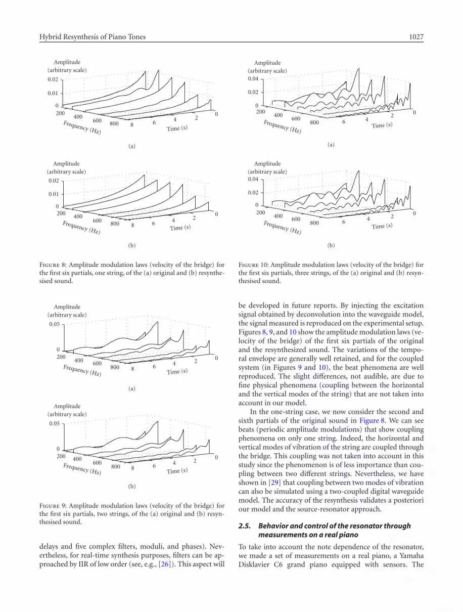
Figure 8: Amplitude modulation laws (velocity of the bridge) forthe first six partials, one string, of the (a) original and (b) resynthe-sised sound.

0

0.05

200400 600

800 8 6 4 2 0

Amplitude(arbitrary scale)

Frequency (Hz) Time (s)

(a)

0

0.05

200 400600

800 8 6 4 20

Amplitude(arbitrary scale)

Frequency (Hz) Time (s)

(b)

Figure 9: Amplitude modulation laws (velocity of the bridge) forthe first six partials, two strings, of the (a) original and (b) resyn-thesised sound.

delays and five complex filters, moduli, and phases). Nev-ertheless, for real-time synthesis purposes, filters can be ap-proached by IIR of low order (see, e.g., [26]). This aspect will

0

0.02

0.04

200400

600800 6 4

2 0

Amplitude(arbitrary scale)

Frequency (Hz)Time (s)

(a)

0

0.02

0.04

200400 600

800 6 4 2 0

Amplitude(arbitrary scale)

Frequency (Hz)Time (s)

(b)

Figure 10: Amplitude modulation laws (velocity of the bridge) forthe first six partials, three strings, of the (a) original and (b) resyn-thesised sound.

be developed in future reports. By injecting the excitationsignal obtained by deconvolution into the waveguide model,the signal measured is reproduced on the experimental setup.Figures 8, 9, and 10 show the amplitude modulation laws (ve-locity of the bridge) of the first six partials of the originaland the resynthesized sound. The variations of the tempo-ral envelope are generally well retained, and for the coupledsystem (in Figures 9 and 10), the beat phenomena are wellreproduced. The slight differences, not audible, are due tofine physical phenomena (coupling between the horizontaland the vertical modes of the string) that are not taken intoaccount in our model.

In the one-string case, we now consider the second andsixth partials of the original sound in Figure 8. We can seebeats (periodic amplitude modulations) that show couplingphenomena on only one string. Indeed, the horizontal andvertical modes of vibration of the string are coupled throughthe bridge. This coupling was not taken into account in thisstudy since the phenomenon is of less importance than cou-pling between two different strings. Nevertheless, we haveshown in [29] that coupling between two modes of vibrationcan also be simulated using a two-coupled digital waveguidemodel. The accuracy of the resynthesis validates a posterioriour model and the source-resonator approach.

2.5. Behavior and control of the resonator throughmeasurements on a real piano

To take into account the note dependence of the resonator,we made a set of measurements on a real piano, a YamahaDisklavier C6 grand piano equipped with sensors. The

1028 EURASIP Journal on Applied Signal Processing

0.7

0.75

0.8

0.85

0.9

0.95

1

0 1000 2000 3000 4000 5000 6000 7000

Frequency (Hz)

Mod

ulu

s

ModeledOriginal

Figure 11: Modulus of the waveguide filters for notes A0, F1 andD3, original and modeled.

vibrations of the strings were measured at the bridge by anaccelerometer, and the hammer velocities were measured bya photonic sensor. Data were collected for several velocitiesand several notes. We used the estimation process describedin Section 2.3 for the previous experimental setup and ex-tracted for each note and each velocity the correspondingresonator and source parameters.

As expected, the behavior of the resonator as a func-tion of the hammer velocity and for a given note is similarto the one described in Section 2.4.2, for the signals mea-sured on the experimental setup. The filters are similar withrespect to the hammer velocity. Their modulus is close toone, but slightly weaker than previously, since it now takesinto account the losses due to the acoustic field radiated bythe soundboard. The resynthesis of the piano measurementsthrough the resonator model and the excitation obtained bydeconvolution are perceptively satisfactory since the sound isalmost indistinguishable from the original one.

On the contrary, the shape of the filters is modified asa function of the note. Figure 11 shows the modulus of thewaveguide filter F for several notes (in the multiple stringcase, we calculated an average filter by arithmetic averaging).The modulus of the loop filter is related to the losses under-gone by the wave over one period. Note that this modulus in-creases with the fundamental frequency, indicating decreas-ing loss over one period as the treble range is approached.

The relations (7) and (8), relating the physical parame-ters to the waveguide parameters, allow the resonator to becontrolled in a relevant physical way. We can either changethe length of the strings, the inharmonicity, or the losses. Butto be in accordance with the physical system, we have to takeinto account the interdependence of some parameters. Forinstance, the fundamental frequency is obviously related tothe length of the string, and to the tension and the linearmass. If we modify the length of the string, we also have to

−3

−2

−1

0

1

2

3

4

0 1 2 3 4 5 6

Time (ms)

Am

plit

ude

(arb

itra

rysc

ale)

0.8 m/s2 m/s4 m/s

Figure 12: Waveform of three excitation signals of the experimentalsetup, corresponding to three different hammer velocities.

modify, for instance, the fundamental frequency, consider-ing that the tension and the linear mass are unchanged. Thisaspect has been taken into account in the implementation ofthe model.

3. THE SOURCE MODEL

In the previous section, we observed that the waveguidefilters are almost invariant with respect to the velocity. Incontrast, the excitation signals (obtained as explained inSection 2.3 and related to the impact of the hammer onthe string) varies nonlinearly as a function of the velocity,thereby taking into account the timbre variations of the re-sulting piano sound. From the extracted excitation signals,we here study the behavior and design a source model byusing signal methods, so as to simulate these behaviors pre-cisely. The source signal is then convolved with the resonatorfilter to obtain the piano bridge signal.

3.1. Nonlinear source behavior as a functionof the hammer velocity

Figure 12 shows the excitation signals extracted from themeasurement of the vibration of a single string struck bya hammer for three velocities corresponding to the pianis-simo, mezzo-forte, and fortissimo musical playing. The exci-tation duration is about 5 milliseconds, which is shorter thanwhat Laroche and Meillier [10] proposed and in accordancewith the duration of the hammer-string contact [6]. Sincethis interaction is nonlinear, the source also behaves nonlin-early. Figure 13 shows the spectra of several excitation signalsobtained for a single string at different velocities regularlyspaced between 0.8 and 4 m/s. The excitation correspond-ing to fortissimo provides more energy than the ones corre-sponding to mezzo-forte and pianissimo. But this increased

Hybrid Resynthesis of Piano Tones 1029

−20

−10

0

10

20

30

40

500 1000 1500 2000 2500 3000 3500 4000 4500

Frequency (Hz)

Am

plit

ude

(dB

)

4 m/s

0.8 m/s

Figure 13: Amplitude of the excitation signals for one string andseveral velocities.

amplitude is frequency dependent: the higher partials in-crease more rapidly than the lower ones with the same ham-mer velocity. This increase in the high partials correspondsto an increase in brightness with respect to the hammer ve-locity. It can be better visualized by considering the spec-tral centroid [31] of the excitation signals. Figure 14 showsthe behavior of this perceptually (brightness) relevant crite-ria [32] as a function of the hammer velocity. Clearly, for one,two, or three strings, the spectral centroid is increased, cor-responding to an increased brightness of the sound. In addi-tion to the change of slope, which translates into the changeof brightness, Figure 13 shows several irregularities commonto all velocities, among which a periodic modulation relatedto the location of the hammer impact on the string.

3.2. Design of a source signal model

The amplitude of the excitation increases smoothly as a func-tion of the hammer velocity. For high-frequency compo-nents, this increase is greater than for low frequency compo-nents, leading to a flattening of the spectrum. Nevertheless,the general shape of the spectrum stays the same. Formantsdo not move and the modulation of the spectrum due to thehammer position on the string is visible at any velocity. Theseobservations suggest that the behavior of the excitation couldbe well reproduced using a subtractive synthesis model.

The excitation signal is seen as an invariant spectrumshaped by a smooth frequency response filter, the charac-teristics of which depend on the hammer velocity. The re-sulting source model is shown on Figure 15. The subtractivesource model consists of the static spectrum, the spectral de-viation, and the gain. The static spectrum takes into accountall the information that is invariant with respect to the ham-mer velocity. It is a function of the characteristics of the ham-mer and the strings. The spectral deviation and the gain bothshape the spectrum as function of the hammer velocity. Thespectral deviation simulates the shifting of the energy to thehigh frequencies, and the gain models the global increase of

1200

1400

1600

1800

2000

2200

1 1.5 2 2.5 3 3.5 4

Hammer velocity (m/s)

Freq

uen

cy(H

z)

One stringTwo stringsThree strings

Figure 14: The spectral centroid of the excitation signals for one(plain), two (dash-dotted) and three (dotted) strings.

Hammer position Hammer velocity

Static spectrum Spectral deviation Gain

0 dBEs E

Figure 15: Diagram of the subtractive source model.

amplitude. Earlier versions of this model were presented in[1, 2]. This type of models has been, in addition, shown towork well for many instruments [33].

In the early days of digital waveguides, Jaffe and Smith[24] modeled the velocity-dependent spectral deviation asa one-pole lowpass filter. Laursen et al. [34] proposed asecond-order biquad filter to model the differences betweenguitar tones with different dynamics.

A similar approach was developed by Smith and VanDuyne in the time domain [15]. The hammer-string interac-tion force pulses were simulated using three impulses passedthrough three lowpass filters which depend on the hammervelocity. In our case, a more accurate method is needed toresynthesize the original excitation signal faithfully.

3.2.1. The static spectrum

We defined the static spectrum as the part of the excitationthat is invariant with the hammer velocity. Considering theexpression of the amplitude of the partials, an, for a hammerstriking a string fixed at its extremities (see Valette and Cuesta[19]), and knowing that the spectrum of the excitation is

1030 EURASIP Journal on Applied Signal Processing

−30

−20

−10

0

10

20

30

1000 2000 3000 4000 5000 6000 7000

Frequency (Hz)

Am

plit

ude

(dB

)

Figure 16: The static spectrum Es(ω).

related to amplitudes of the partials by E = anD [29], thestatic spectrum Es can be expressed as

Es(ωn) = 4L

T

sin(nπx0/L

)nπ√

1 + n2B, (12)

where T is the string tension and L its length, B is the inhar-monicity factor, and x0 the striking position. We can easilymeasure the striking position, the string length and the in-harmonicity factor on our experimental setup. On the otherhand, we have an only estimation of the tension, it can becalculated through the fundamental frequency and the linearmass of the string.

Figure 16 shows this static spectrum for a single string.Many irregularities, however, are not taken into account forseveral reasons. We will see later their importance from a per-ceptual point of view. Equation (12) is still used, however,when the hammer position is changed. This is useful whenone plays with a different temperament because it reducesdissonance.

3.2.2. The deviation with the dynamic

The spectral deviation and the gain take into account the de-pendency of the excitation signal on velocity. They are esti-mated by dividing the spectrum of the excitation signal bythe static spectrum for all velocities:

d(ω) = E(ω)Es(ω)

, (13)

where E is the original excitation signal. Figure 17 shows thisdeviation for three hammer velocities. It effectively strength-ens the fortissimo, in particular for the medium and highpartials. Its evolution with the frequency is regular and cansuccessfully be fitted to a first-order exponential polynomial(as shown in Figure 17)

d = exp(a f + g), (14)

−70

−60

−50

−40

−30

−20

−10

0

10

20

0 2000 4000 6000 8000 10000

Frequency (Hz)

Am

plit

ude

(dB

)

OriginalSpectral tilt

3.8 m/s

2.0 m/s

0.8 m/s

Figure 17: Dynamic deviation of three excitation signals of the ex-perimental setup, original and modeled.

35

40

45

50

0 1 2 3 4 5 6

dB

Hammer velocity (m/s)

5

10

15

20

0 1 2 3 4 5 6

dB/k

Hz

Hammer velocity (m/s)

Figure 18: Parameters g (gain)(top), a (spectral deviation) (bot-tom) as a function of the hammer velocity for the experimentalsetup signals, original (+) and modeled (dashed).

where d is the modeled deviation. The term g correspondsto the gain (independent of the frequency) and the term a fcorresponds to the spectral deviation. The variables g anda depend on the hammer velocity. To get a usable sourcemodel, we must consider the parameter’s behavior with dif-ferent dynamics. Figure 18 shows the two parameters for sev-eral hammer velocities. The model is consistent since theirbehavior is regular. But the tilt increases with the hammer ve-locity, showing an asymptotic and nonlinear behavior. Thisobservation can be directly related to the physics of the ham-mer. As we have seen, when the felt is compressed, it be-comes harder and thus gives more energy to high frequen-cies. But, for high velocities, the felt is totally compressed andits hardness is almost constant. Thus, the amplitude of the

Hybrid Resynthesis of Piano Tones 1031

corresponding string wave increases further but its spectralcontent is roughly the same. We have fitted this asymptoticbehavior by an exponential model (see Figure 18), for eachparameter g and a,

g(v) = αg − βg exp(− γgv

),

a(v) = αa − βa exp(− γav

),

(15)

where αi (i = g, a) is the asymptotic value, βi (i = g, a) isthe deviation from the asymptotic value at zero velocity (thedynamic range), and γi (i = g, a) is the velocity exponen-tial coefficient, governing how sensitive the attribute is to avelocity change. The parameters of this exponential modelwere found using a nonlinear weighted curvefit.

3.2.3. Resynthesis of the excitation signal

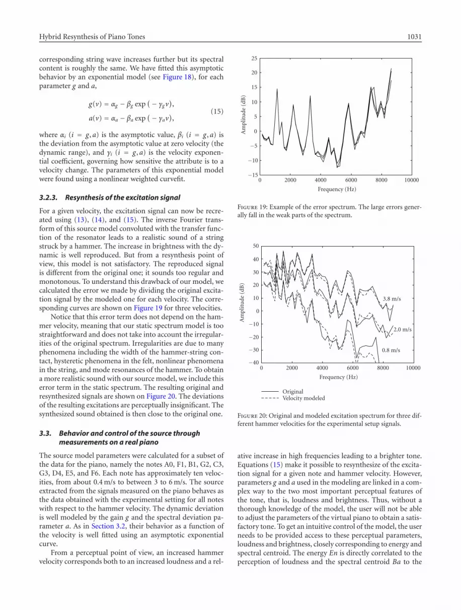
For a given velocity, the excitation signal can now be recre-ated using (13), (14), and (15). The inverse Fourier trans-form of this source model convoluted with the transfer func-tion of the resonator leads to a realistic sound of a stringstruck by a hammer. The increase in brightness with the dy-namic is well reproduced. But from a resynthesis point ofview, this model is not satisfactory. The reproduced signalis different from the original one; it sounds too regular andmonotonous. To understand this drawback of our model, wecalculated the error we made by dividing the original excita-tion signal by the modeled one for each velocity. The corre-sponding curves are shown on Figure 19 for three velocities.

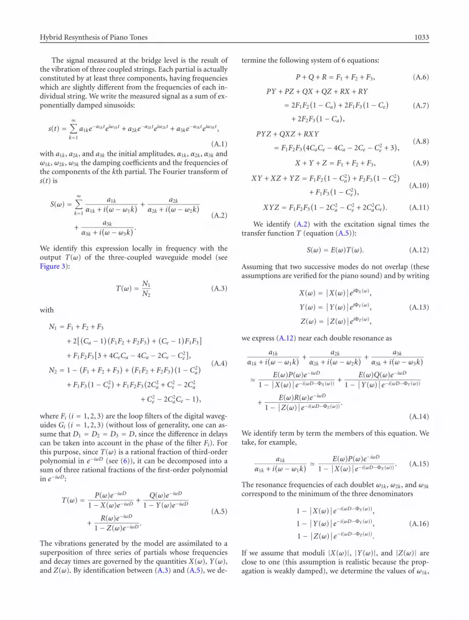
Notice that this error term does not depend on the ham-mer velocity, meaning that our static spectrum model is toostraightforward and does not take into account the irregular-ities of the original spectrum. Irregularities are due to manyphenomena including the width of the hammer-string con-tact, hysteretic phenomena in the felt, nonlinear phenomenain the string, and mode resonances of the hammer. To obtaina more realistic sound with our source model, we include thiserror term in the static spectrum. The resulting original andresynthesized signals are shown on Figure 20. The deviationsof the resulting excitations are perceptually insignificant. Thesynthesized sound obtained is then close to the original one.

3.3. Behavior and control of the source throughmeasurements on a real piano

The source model parameters were calculated for a subset ofthe data for the piano, namely the notes A0, F1, B1, G2, C3,G3, D4, E5, and F6. Each note has approximately ten veloc-ities, from about 0.4 m/s to between 3 to 6 m/s. The sourceextracted from the signals measured on the piano behaves asthe data obtained with the experimental setting for all noteswith respect to the hammer velocity. The dynamic deviationis well modeled by the gain g and the spectral deviation pa-rameter a. As in Section 3.2, their behavior as a function ofthe velocity is well fitted using an asymptotic exponentialcurve.

From a perceptual point of view, an increased hammervelocity corresponds both to an increased loudness and a rel-

−15

−10

−5

0

5

10

15

20

25

0 2000 4000 6000 8000 10000

Frequency (Hz)

Am

plit

ude

(dB

)

Figure 19: Example of the error spectrum. The large errors gener-ally fall in the weak parts of the spectrum.

−40

−30

−20

−10

0

10

20

30

40

50

0 2000 4000 6000 8000 10000

Frequency (Hz)

Am

plit

ude

(dB

)

3.8 m/s

2.0 m/s

0.8 m/s

OriginalVelocity modeled

Figure 20: Original and modeled excitation spectrum for three dif-ferent hammer velocities for the experimental setup signals.

ative increase in high frequencies leading to a brighter tone.Equations (15) make it possible to resynthesize of the excita-tion signal for a given note and hammer velocity. However,parameters g and a used in the modeling are linked in a com-plex way to the two most important perceptual features ofthe tone, that is, loudness and brightness. Thus, without athorough knowledge of the model, the user will not be ableto adjust the parameters of the virtual piano to obtain a satis-factory tone. To get an intuitive control of the model, the userneeds to be provided access to these perceptual parameters,loudness and brightness, closely corresponding to energy andspectral centroid. The energy En is directly correlated to theperception of loudness and the spectral centroid Ba to the

1032 EURASIP Journal on Applied Signal Processing

perception of brightness [32]. These parameters are given by

En = 1T

∫ Fs/2

0E2( f )df ,

Ba =∫ Fs/2

0 E( f ) f df∫ Fs/20 E( f )df

,

(16)

where f is the frequency and Fs the sampling frequency.To synthesize an excitation signal having a given energy

and spectral centroid, we must express parameters g and a asfunctions of Ba and En. The centroid actually depends onlyon a:

Ba =∫ Fs/2

0 Es( f )ea f f df∫ Fs/20 Es( f )ea f df

. (17)

We numerically calculate the expression of a as a function ofBa and store the solution in a table. Alternatively, assumingthat the brightness change is unaffected by the shape of thestatic spectrum Es, the spectral deviation parameter a can becalculated directly from the given brightness [35].

Knowing a, we can calculate g from the energy En by therelation

g = 12

log

(EnT∫ Fs/2

0 Es2( f )e2a f 2+2b f

). (18)

The behavior of Ba and En as a function of the hammervelocity will then determine the dynamic range of the instru-ment and it must be defined by the user.

Figure 21 shows the behavior of the spectral centroid andthe energy for several notes. The curves have similar behaviorand differ mainly by a multiplicative constant. We have fittedtheir asymptotic behavior by an exponential model, similarlyto what was done with (15). These functions are applied tothe synthesis of each excitation signal and then characterizethe dynamic range of the virtual instrument. It is easy for theuser to change the dynamic range of the virtual instrument,which is modified by the user by changing the shape of thesefunctions.

Calculating the excitation signal is then done as follows.To a given note and velocity, we associate a spectral centroidBa and an energy En (using the asymptotic exponential fit);a is then obtained from the spectral centroid and g from theenergy (equation (18)). One finally gets the spectral devia-tion which, multiplied by the static spectrum, allows the ex-citation signal to be calculated.

4. CONCLUSION

The reproduction of the piano bridge vibration is undoubtlythe first most important step for piano sound synthesis. Weshow that a hybrid model consisting of a resonant part andan excitation part is well adapted for this purpose. After accu-rate calibration, the sounds obtained are perceptually close tothe original ones for all notes and velocities. The resonator,which simulates the phenomena intervening in the strings

1000

2000

3000

4000

5000

6000

1 2 3 4 5 6

Freq

uen

cy(H

z)

Hammer velocity (m/s)

F6

E5D4

G3C3

F1 G2B1A0

(a)

0

20

40

60

1 2 3 4 5 6

F6E5

D4G3C3G2B1

F1A0

dBHammer velocity (m/s)

(b)

Figure 21: Spectral centroid (a) and energy (b) for several notesas a function of the hammer velocity, original (plain) and modeled(dotted).

themselves, is modeled by a digital waveguide model that isvery efficient in simulating the wave propagation. The res-onator model exhibits physical parameters such as the stringtension, the inharmonicity coefficient, allowing physicallyrelevant control of the resonator. It also takes into accountthe coupling effects, which are extremely relevant for percep-tion. The source is extracted using a deconvolution processand is modeled using a subtractive signal model. The sourcemodel consists of three parts (static spectrum, spectral devi-ation, and gain) that are dependent on the velocities and thenotes played. To get intuitive control of the source model, weexhibited two parameters: the spectral centroid and the en-ergy, strongly related to the perceptual parameters brightnessand loudness. This perceptual link permits easy control of thedynamic characteristics of the piano.

Thus, the tone of a given piano can be synthesized using ahybrid model. This model is currently implemented in real-time using a Max-MSP software environment.

APPENDIX

INVERSE PROBLEM, THREE-COUPLEDDIGITAL WAVEGUIDE

We show in this appendix how the parameters of a three-coupled digital waveguide model can be expressed as func-tion of the modal parameters. This method is an extensionof the model presented in [29].

Hybrid Resynthesis of Piano Tones 1033

The signal measured at the bridge level is the result ofthe vibration of three coupled strings. Each partial is actuallyconstituted by at least three components, having frequencieswhich are slightly different from the frequencies of each in-dividual string. We write the measured signal as a sum of ex-ponentially damped sinusoids:

s(t) =∞∑k=1

a1ke−α1kteiω1kt + a2ke

−α2kteiω2kt + a3ke−α3kteiω3kt,

(A.1)with a1k, a2k, and a3k the initial amplitudes, α1k, α2k, α3k andω1k, ω2k, ω3k the damping coefficients and the frequencies ofthe components of the kth partial. The Fourier transform ofs(t) is

S(ω) =∞∑k=1

a1k

α1k + i(ω − ω1k

) +a2k

α2k + i(ω− ω2k

)+

a3k

α3k + i(ω − ω3k

) .(A.2)

We identify this expression locally in frequency with theoutput T(ω) of the three-coupled waveguide model (seeFigure 3):

T(ω) = N1

N2(A.3)

with

N1 = F1 + F2 + F3

+ 2[(Ca − 1

)(F1F2 + F2F3

)+(Ce − 1

)F1F3

]+ F1F2F3

[3 + 4CeCa − 4Ca − 2Ce − C2

e

],

N2 = 1− (F1 + F2 + F3)

+(F1F2 + F2F3

)(1− C2

a

)+ F1F3

(1− C2

e

)+ F1F2F3

(2C2

a + C2e − 2C2

a

+ C2e − 2C2

aCe − 1),

(A.4)

where Fi (i = 1, 2, 3) are the loop filters of the digital waveg-uides Gi (i = 1, 2, 3) (without loss of generality, one can as-sume that D1 = D2 = D3 = D, since the difference in delayscan be taken into account in the phase of the filter Fi). Forthis purpose, since T(ω) is a rational fraction of third-orderpolynomial in e−iωD (see (6)), it can be decomposed into asum of three rational fractions of the first-order polynomialin e−iωD:

T(ω) = P(ω)e−iωD

1− X(ω)e−iωD+

Q(ω)e−iωD

1− Y(ω)e−iωD

+R(ω)e−iωD

1− Z(ω)e−iωD.

(A.5)

The vibrations generated by the model are assimilated to asuperposition of three series of partials whose frequenciesand decay times are governed by the quantities X(ω), Y(ω),and Z(ω). By identification between (A.3) and (A.5), we de-

termine the following system of 6 equations:

P + Q + R = F1 + F2 + F3, (A.6)

PY + PZ + QX + QZ + RX + RY

= 2F1F2(1− Ca

)+ 2F1F3

(1− Ce

)+ 2F2F3

(1− Ca

),

(A.7)

PYZ + QXZ + RXY

= F1F2F3(4CaCe − 4Ca − 2Ce − C2

e + 3),

(A.8)

X + Y + Z = F1 + F2 + F3, (A.9)

XY + XZ + YZ = F1F2(1− C2

a

)+ F2F3

(1− C2

a

)+ F1F3

(1− C2

e

),

(A.10)

XYZ = F1F2F3(1− 2C2

a − C2e + 2C2

aCe). (A.11)

We identify (A.2) with the excitation signal times thetransfer function T (equation (A.5)):

S(ω) = E(ω)T(ω). (A.12)

Assuming that two successive modes do not overlap (theseassumptions are verified for the piano sound) and by writing

X(ω) = ∣∣X(ω)∣∣eiΦX (ω),

Y(ω) = ∣∣Y(ω)∣∣eiΦY (ω),

Z(ω) = ∣∣Z(ω)∣∣eiΦZ (ω),

(A.13)

we express (A.12) near each double resonance as

a1k

α1k + i(ω− ω1k

) +a2k

α2k + i(ω − ω2k

) +a3k

α3k + i(ω − ω3k

)� E(ω)P(ω)e−iωD

1− ∣∣X(ω)∣∣e−i(ωD−ΦX (ω))

+E(ω)Q(ω)e−iωD

1− ∣∣Y(ω)∣∣e−i(ωD−ΦY (ω))

+E(ω)R(ω)e−iωD

1− ∣∣Z(ω)∣∣e−i(ωD−ΦZ (ω))

.

(A.14)

We identify term by term the members of this equation. Wetake, for example,

a1k

α1k + i(ω − ω1k

) � E(ω)P(ω)e−iωD

1− ∣∣X(ω)∣∣e−i(ωD−ΦX (ω))

. (A.15)

The resonance frequencies of each doublet ω1k, ω2k, and ω3k

correspond to the minimum of the three denominators

1− ∣∣X(ω)∣∣e−i(ωD−ΦX (ω)),

1− ∣∣Y(ω)∣∣e−i(ωD−ΦY (ω)),

1− ∣∣Z(ω)∣∣e−i(ωD−ΦZ (ω)).

(A.16)

If we assume that moduli |X(ω)|, |Y(ω)|, and |Z(ω)| areclose to one (this assumption is realistic because the prop-agation is weakly damped), we determine the values of ω1k,

1034 EURASIP Journal on Applied Signal Processing

ω2k, and ω3k:

ω1k = ΦX(ω1k

)+ 2kπ

D,

ω2k = ΦY(ω2k

)+ 2kπ

D,

ω3k = ΦZ(ω3k

)+ 2kπ

D.

(A.17)

Taking ω = ω1k + ε with ε arbitrary small,

a1k

α1k + iε� E

(ω1k + ε

)P(ω1k + ε

)e−iΦX (ω1k+ε)e−iεD

1− ∣∣X(ω1k + ε)∣∣e−iεD . (A.18)

A limited expansion of e−iεD � 1− iεD+ θ(ε2) around ε = 0(at the zeroth order for the numerator and at the first orderfor the denominator) gives

E(ω1k + ε

)P(ω1k + ε

)e−iΦX (ω1k+ε)e−iεD

� E(ω1k

)P(ω1k

)e−iΦX (ω1k),

1− ∣∣X(ω1k + ε)∣∣e−iεD � 1− ∣∣X(ω1k

)∣∣(1− iεD).

(A.19)

Assuming that P(ω) and |X(ω)| are locally constant (in thefrequency domain), we identify term by term (the two mem-bers are considered as functions of the variable ε). We deducethe expressions of |X(ω)|, |Y(ω)|, and |Z(ω)| as a functionof the amplitudes and decay times coefficients for each mode:

∣∣X(ω1k)∣∣ = 1

α1kD + 1,

∣∣Y(ω2k)∣∣ = 1

α2kD + 1,

∣∣Z(ω2k)∣∣ = 1

α3kD + 1.

(A.20)

We also get the relations

E(ω1k

)P(ω1k

) = a1kDX(ω1k

),

E(ω2k

)Q(ω2k

) = a2kDY(ω2k

),

E(ω3k

)Q(ω3k

) = a3kDY(ω3k

).

(A.21)

From the measured signal, we estimate the modal parame-ters a1k, a2k, a3k, α1k, α2k, α3k, ω1k, ω2k, and ω3k. Using (A.17)and (A.20), we calculate X , Y , and Z. We still have 9 un-known variables P, Q, R, E, Ca, Ce, F1, F2, and F3. But wealso have a system of 9 equations ((A.6), (A.7), (A.8), (A.9),(A.10), (A.11), and (A.21)). Assuming that the two resonancefrequencies are close and that the variables P, Q, R, E, Ca,Ce, F1, F2, F3, X , Y , and Z have a locally smooth behav-ior, we then express the waveguide parameters as function ofthe temporal parameters. For the sake of simplicity, we noteEk = E(ω1k) = E(ω2k).

Using (A.6) and (A.9), we obtain Pk + Qk + Rk = Xk +Yk +Zk. Thanks to (A.21) we finally get the expression of theexcitation signal at the resonance frequencies

Ek = D(a1kXk + a2kYk + a3kZk

)Xk + Yk + Zk

. (A.22)

In the case of a two-coupled digital waveguide, the corre-sponding system admits analytical solutions (see [29]). Butin the case of three-coupled digital waveguide, we have notfound analytical expressions for variables P, Q, R, Ca, Ce, F1,F2, and F3. We have then solved the system numerically.

REFERENCES

[1] J. Bensa, K. Jensen, R. Kronland-Martinet, and S. Ystad, “Per-ceptual and analytical analysis of the effect of the hammer im-pact on piano tones,” in Proc. International Computer MusicConference, pp. 58–61, Berlin, Germany, August 2000.

[2] J. Bensa, F. Gibaudan, K. Jensen, and R. Kronland-Martinet,“Note and hammer velocity dependance of a piano stringmodel based on coupled digital waveguides,” in Proc. Interna-tional Computer Music Conference, pp. 95–98, Havana, Cuba,September 2001.

[3] A. Askenfelt, Ed., Five Lectures on the Acoustics of the Pi-ano, Royal Swedish Academy of Music, Stockholm, Swe-den, 1990, Lectures by H. A. Conklin, Anders Askenfeltand E. Jansson, D. E. Hall, G. Weinreich, and K. Wogram,http://www.speech.kth.se/music/5 lectures/.

[4] S. Ystad, Sound modeling using a combination of physical andsignal models, Ph.D. thesis, Universite de la Mediterranee,Marseille, France, 1998.

[5] S. Ystad, “Sound modeling applied to flute sounds,” Journalof the Audio Engineering Society, vol. 48, no. 9, pp. 810–825,2000.

[6] A. Askenfelt and E. V. Jansson, “From touch to string vibra-tions. II: The motion of the key and hammer,” Journal of theAcoustical Society of America, vol. 90, no. 5, pp. 2383–2393,1991.

[7] A. Askenfelt and E. V. Jansson, “From touch to string vibra-tions. III: String motion and spectra,” Journal of the AcousticalSociety of America, vol. 93, no. 4, pp. 2181–2195, 1993.

[8] X. Boutillon, “Le piano: Modelisation physiques et devel-oppements technologiques,” in Congres Francais d’AcoustiqueColloque C2, pp. 811–820, Lyon, France, 1990.

[9] P. Schaeffer, Traite des objets musicaux, Edition du Seuil, Paris,France, 1966.

[10] J. Laroche and J. L. Meillier, “Multichannel excitation/filtermodeling of percussive sounds with application to the piano,”IEEE Trans. Speech and Audio Processing, vol. 2, no. 2, pp. 329–344, 1994.

[11] J. O. Smith III, “Physical modeling using digital waveguides,”Computer Music Journal, vol. 16, no. 4, pp. 74–91, 1992.

[12] G. Borin, D. Rochesso, and F. Scalcon, “A physical pianomodel for music performance,” in Proc. International Com-puter Music Conference, pp. 350–353, Computer Music Asso-ciation, Thessaloniki, Greece, September 1997.

[13] B. Bank, “Physics-based sound synthesis of the piano,” M.S.thesis, Budapest University of Technology and Economics,Budapest, Hungary, 2000, published as Report 54, HelsinkiUniversity of Technology, Laboratory of Acoustics and AudioSignal Processing, http://www.mit.bme.hu/∼bank.

[14] J. O. Smith III, “Efficient synthesis of stringed musical instru-ments,” in Proc. International Computer Music Conference, pp.64–71, Computer Music Association, Tokyo, Japan, Septem-ber 1993.

[15] J. O. Smith III and S. A. Van Duyne, “Commuted piano syn-thesis,” in Proc. International Computer Music Conference,pp. 335–342, Computer Music Association, Banff, Canada,September 1995.

[16] S. A. Van Duyne and J. O. Smith III, “Developments forthe commuted piano,” in Proc. International Computer Music

Hybrid Resynthesis of Piano Tones 1035

Conference, pp. 319–326, Computer Music Association, Banff,Canada, September 1995.

[17] A. Chaigne and A. Askenfelt, “Numerical simulations ofstruck strings. I. A physical model for a struck string usingfinite difference methods,” Journal of the Acoustical Society ofAmerica, vol. 95, no. 2, pp. 1112–1118, 1994.

[18] X. Boutillon, “Model for piano hammers: Experimental de-termination and digital simulation,” Journal of the AcousticalSociety of America, vol. 83, no. 2, pp. 746–754, 1988.

[19] C. Valette and C. Cuesta, Mecanique de la corde vibrante,Traite des nouvelles technologies. Serie Mecanique. Hermes,Paris, France, 1993.

[20] D. E. Hall and A. Askenfelt, “Piano string excitation V: Spectrafor real hammers and strings,” Journal of the Acoustical Societyof America, vol. 83, no. 6, pp. 1627–1638, 1988.

[21] J. Bensa, S. Bilbao, R. Kronland-Martinet, and J. O. SmithIII, “The simulation of piano string vibration: from physi-cal model to finite difference schemes and digital waveguides,”Journal of the Acoustical Society of America, vol. 114, no. 2, pp.1095–1107, 2003.

[22] A. Chaigne and V. Doutaut, “Numerical simulations of xy-lophones. I. Time-domain modeling of the vibration bars,”Journal of the Acoustical Society of America, vol. 101, no. 1, pp.539–557, 1997.

[23] H. Fletcher, E. D. Blackham, and R. Stratton, “Quality of pi-ano tones,” Journal of the Acoustical Society of America, vol.34, no. 6, pp. 749–761, 1962.

[24] D. A. Jaffe and J. O. Smith III, “Extensions of the Karplus-Strong plucked-string algorithm,” Computer Music Journal,vol. 7, no. 2, pp. 56–69, 1983.

[25] G. Weinreich, “Coupled piano strings,” Journal of the Acous-tical Society of America, vol. 62, no. 6, pp. 1474–1484, 1977.

[26] V. Valimaki, J. Huopaniemi, M. Karjalainen, and Z. Janosy,“Physical modeling of plucked string instruments with appli-cation to real-time sound synthesis,” Journal of the Audio En-gineering Society, vol. 44, no. 5, pp. 331–353, 1996.

[27] B. Bank, “Accurate and efficient modeling of beating and two-stage decay for string instrument synthesis,” in Proc. Workshopon Current Research Directions in Computer Music, pp. 134–137, Barcelona, Spain, November 2001.

[28] D. Rocchesso and J. O. Smith III, “Generalized digital waveg-uide networks,” IEEE Trans. Speech and Audio Processing, vol.11, no. 3, pp. 242–254, 2003.

[29] M. Aramaki, J. Bensa, L. Daudet, P. Guillemain, andR. Kronland-Martinet, “Resynthesis of coupled piano stringvibrations based on physical modeling,” Journal of New MusicResearch, vol. 30, no. 3, pp. 213–226, 2002.

[30] K. Steiglitz and L. E. McBride, “A technique for the identifi-cation of linear systems,” IEEE Trans. Automatic Control, vol.10, pp. 461–464, 1965.

[31] J. Beauchamp, “Synthesis by spectral amplitude and “bright-ness” matching of analyzed musical instrument tones,” Jour-nal of the Audio Engineering Society, vol. 30, no. 6, pp. 396–406, 1982.

[32] S. McAdams, S. Winsberg, S. Donnadieu, G. de Soete, andJ. Krimphoff, “Perceptual scaling of synthesized musical tim-bres: Common dimensions, specificities, and latent subjectclasses,” Psychological Research, vol. 58, pp. 177–192, 1992.

[33] K. Jensen, “Musical instruments parametric evolution,” inProc. International Symposium on Musical Acoustics, pp. 319–326, Computer Music Association, Mexico City, Mexico, De-cember 2002.

[34] M. Laursen, C. Erkut, V. Valimaki, and M. Kuuskankara,“Methods for modeling realistic playing in acoustic guitarsynthesis,” Computer Music Journal, vol. 25, no. 3, pp. 38–49,2001.

[35] K. Jensen, Timbre models of musical sounds, Ph.D. thesis,Department of Datalogy, University of Copenhagen, Copen-hagen, Denmark, DIKU Tryk, Technical Report No 99/7,1999.

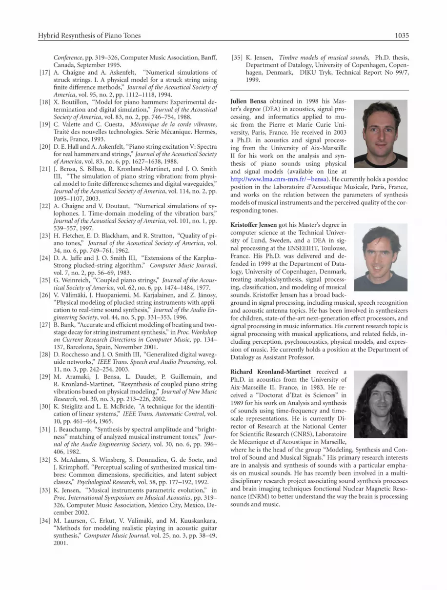
Julien Bensa obtained in 1998 his Mas-ter’s degree (DEA) in acoustics, signal pro-cessing, and informatics applied to mu-sic from the Pierre et Marie Curie Uni-versity, Paris, France. He received in 2003a Ph.D. in acoustics and signal process-ing from the University of Aix-MarseilleII for his work on the analysis and syn-thesis of piano sounds using physicaland signal models (available on line athttp://www.lma.cnrs-mrs.fr/∼bensa). He currently holds a postdocposition in the Laboratoire d’Acoustique Musicale, Paris, France,and works on the relation between the parameters of synthesismodels of musical instruments and the perceived quality of the cor-responding tones.

Kristoffer Jensen got his Master’s degree incomputer science at the Technical Univer-sity of Lund, Sweden, and a DEA in sig-nal processing at the ENSEEIHT, Toulouse,France. His Ph.D. was delivered and de-fended in 1999 at the Department of Data-logy, University of Copenhagen, Denmark,treating analysis/synthesis, signal process-ing, classification, and modeling of musicalsounds. Kristoffer Jensen has a broad back-ground in signal processing, including musical, speech recognitionand acoustic antenna topics. He has been involved in synthesizersfor children, state-of the-art next-generation effect processors, andsignal processing in music informatics. His current research topic issignal processing with musical applications, and related fields, in-cluding perception, psychoacoustics, physical models, and expres-sion of music. He currently holds a position at the Department ofDatalogy as Assistant Professor.

Richard Kronland-Martinet received aPh.D. in acoustics from the University ofAix-Marseille II, France, in 1983. He re-ceived a “Doctorat d’Etat es Sciences” in1989 for his work on Analysis and synthesisof sounds using time-frequency and time-scale representations. He is currently Di-rector of Research at the National Centerfor Scientific Research (CNRS), Laboratoirede Mecanique et d’Acoustique in Marseille,where he is the head of the group “Modeling, Synthesis and Con-trol of Sound and Musical Signals.” His primary research interestsare in analysis and synthesis of sounds with a particular empha-sis on musical sounds. He has recently been involved in a multi-disciplinary research project associating sound synthesis processesand brain imaging techniques fonctional Nuclear Magnetic Reso-nance (fNRM) to better understand the way the brain is processingsounds and music.

Photograph © Turisme de Barcelona / J. Trullàs

Preliminary call for papers

The 2011 European Signal Processing Conference (EUSIPCO 2011) is thenineteenth in a series of conferences promoted by the European Association forSignal Processing (EURASIP, www.eurasip.org). This year edition will take placein Barcelona, capital city of Catalonia (Spain), and will be jointly organized by theCentre Tecnològic de Telecomunicacions de Catalunya (CTTC) and theUniversitat Politècnica de Catalunya (UPC).EUSIPCO 2011 will focus on key aspects of signal processing theory and

li ti li t d b l A t f b i i ill b b d lit

Organizing Committee

Honorary ChairMiguel A. Lagunas (CTTC)

General ChairAna I. Pérez Neira (UPC)

General Vice ChairCarles Antón Haro (CTTC)

Technical Program ChairXavier Mestre (CTTC)

Technical Program Co Chairsapplications as listed below. Acceptance of submissions will be based on quality,relevance and originality. Accepted papers will be published in the EUSIPCOproceedings and presented during the conference. Paper submissions, proposalsfor tutorials and proposals for special sessions are invited in, but not limited to,the following areas of interest.

Areas of Interest

• Audio and electro acoustics.• Design, implementation, and applications of signal processing systems.

l d l d d

Technical Program Co ChairsJavier Hernando (UPC)Montserrat Pardàs (UPC)

Plenary TalksFerran Marqués (UPC)Yonina Eldar (Technion)

Special SessionsIgnacio Santamaría (Unversidadde Cantabria)Mats Bengtsson (KTH)

FinancesMontserrat Nájar (UPC)• Multimedia signal processing and coding.

• Image and multidimensional signal processing.• Signal detection and estimation.• Sensor array and multi channel signal processing.• Sensor fusion in networked systems.• Signal processing for communications.• Medical imaging and image analysis.• Non stationary, non linear and non Gaussian signal processing.

Submissions

Montserrat Nájar (UPC)

TutorialsDaniel P. Palomar(Hong Kong UST)Beatrice Pesquet Popescu (ENST)

PublicityStephan Pfletschinger (CTTC)Mònica Navarro (CTTC)

PublicationsAntonio Pascual (UPC)Carles Fernández (CTTC)

I d i l Li i & E hibiSubmissions

Procedures to submit a paper and proposals for special sessions and tutorials willbe detailed at www.eusipco2011.org. Submitted papers must be camera ready, nomore than 5 pages long, and conforming to the standard specified on theEUSIPCO 2011 web site. First authors who are registered students can participatein the best student paper competition.

Important Deadlines:

P l f i l i 15 D 2010

Industrial Liaison & ExhibitsAngeliki Alexiou(University of Piraeus)Albert Sitjà (CTTC)

International LiaisonJu Liu (Shandong University China)Jinhong Yuan (UNSW Australia)Tamas Sziranyi (SZTAKI Hungary)Rich Stern (CMU USA)Ricardo L. de Queiroz (UNB Brazil)

Webpage: www.eusipco2011.org

Proposals for special sessions 15 Dec 2010Proposals for tutorials 18 Feb 2011Electronic submission of full papers 21 Feb 2011Notification of acceptance 23 May 2011Submission of camera ready papers 6 Jun 2011