Computers & Operations Research 35 (2008) 1084–1098www.elsevier.com/locate/cor

A hybrid genetic heuristic for scheduling parallel batch processingmachines with arbitrary job sizes

Ali Husseinzadeh Kashan, Behrooz Karimi∗, Masoud JenabiDepartment of Industrial Engineering, Amirkabir University of Technology, 424 Hafez Ave., Tehran 15916-34311, Iran

Available online 17 August 2006

Abstract

This paper investigates the scheduling problem of parallel identical batch processing machines in which each machine can processa group of jobs simultaneously as a batch. Each job is characterized by its size and processing time. The processing time of a batchis given by the longest processing time among all jobs in the batch. Based on developing heuristic approaches, we proposed a hybridgenetic heuristic (HGH) to minimize makespan objective. To verify the performance of our algorithm, comparisons are made throughusing a simulated annealing (SA) approach addressed in the literature as a comparator algorithm. Computational experiments revealthat affording the knowledge of problem through using heuristic procedures, gives HGH the ability of finding optimal or near optimalsolutions in a reasonable time.� 2006 Elsevier Ltd. All rights reserved.

Keywords: Scheduling; Parallel batch processing machines; Genetic algorithm; Simulated annealing

1. Introduction

This paper addresses the problem of scheduling n jobs on m identical parallel batch processing machines. A batchprocessing machine is capable to accommodate a group of jobs simultaneously. Once processing of a batch is initiated,it cannot be interrupted and other jobs cannot be introduced into the machine until processing is completed. With eachjob i we shall associate an arbitrary size si and an arbitrary processing time pi . Each batch processing machine hasa capacity B, so the sum of job sizes in each batch must be less than or equal to B. We assume that no job has a sizeexceeding the machine capacity and it cannot be split across batches.

This research is motivated by burn-in operation in semiconductor manufacturing [1]. The purpose of burn-in operationis to test the integrated circuits by subjecting them to thermal stress for an extended period. The burn-in oven has alimited capacity and sub-grouping the boards holding the circuits in to batches would be inevitable. So, using all or asmuch available space in the processor maximizes efficiency. The processing times of burn-in operations are generallylonger compared to those of other testing operations, so the burn-in operations constitute a bottleneck in the final testingoperation and optimal scheduling of the burn-in operations is of great concern in productivity and on-time deliverymanagement.

In scheduling problems, makespan (Cmax) is equivalent to the completion time of the last job leaving the system.The small Cmax usually implies a high utilization. The utilization for bottleneck station is closely related to throughput

∗ Corresponding author. Tel.: +98 21 66413034; fax: +98 21 66413025.E-mail address: b.karimi@aut.ac.ir (B. Karimi).

0305-0548/$ - see front matter � 2006 Elsevier Ltd. All rights reserved.doi:10.1016/j.cor.2006.07.005

A.H. Kashan et al. / Computers & Operations Research 35 (2008) 1084–1098 1085

rate of the system. Therefore, reducing the Cmax should also lead to a higher throughput rate. This concern led us toconsider the makespan performance measure as the scheduling objective.

The structure of the paper is as follows. In Section 2, we review related works on scheduling models of batchprocessing machines. Section 3 examines the combinatorial complexity of the problem under the considered assump-tions. Sections 4 and 5, respectively, deal with the proposed lower bound and a heuristic approach developed for theproblem. The proposed hybrid genetic heuristic (HGH) and its implementation is presented in Section 6. Section 7deals with the effectiveness of the HGH compared to the SA comparator algorithm. The paper will be concluded inSection 8.

2. Previous related works

Problems related to scheduling batch processing machines, in which machine has the ability of processing a numberof jobs simultaneously, have been examined extensively by many researchers in recent years. Ikura and Gimple [2]probably are the first who addressed scheduling with batch processors. Given identical job processing times, theyproposed an O(n2) algorithm for the problem of determining whether a schedule exists in which all the due datescan be met, when release times and due dates are agreeable. Lee et al. [1] considered minimizing maximum lateness,Lmax, and number of tardy jobs, �Ui , under the same assumptions. Li and Lee [3] showed that these problems are bothstrongly NP-hard, if release times and due dates are not agreeable.

There are number of researches concerned with scheduling burn-in ovens in semiconductor manufacturing industry.In such these operations, the batch processing time depends to batch content and is given by the processing time ofthe longest job in the batch. Lee et al. [1], the first researchers who popularized scheduling burn-in operations, gaveefficient algorithms for minimizing Lmax and �Ui , assuming agreeable processing times and due dates. Brucker et al.[4] gave several exact algorithms and complexity results for the case of infinite machine capacity. For the limited case,they proved that due date-based scheduling criteria give rise to NP-hard problems and provided an O(nB(B−1)) exactalgorithm for minimizing �Ci . Chandru et al. [5] provided heuristics and a branch-and-bound method for minimizing�Ci that can be implemented for solving problems with up to 35 jobs. Adding some new elimination rules, Dupontand Jolai Ghazvini [6] made their method useful for the problems with up to 100 jobs. Uzsoy and Yang [7] studiedthe problem of minimizing total weighted completion time, �wiCi , and provided some heuristics and a branch-and-bound algorithm. Lee and Uzsoy [8] studied the problem of minimizing Cmax in the presence of dynamic job arrivals.Scheduling a single batch processing machine where boards are also considered as a secondary resource constraint hasbeen considered by Kempf et al. [9].

Scheduling batching machines with incompatible job families, i.e. when the processing times of all jobs in the samefamily are equal and jobs of different families cannot be processed together in the same batch, has been addressed byresearchers. Uzsoy [10] developed efficient algorithms for minimizing Lmax and �wiCi on a single batch processingmachine. He also addressed the problems of minimizing Cmax and Lmax in the presence of dynamic job arrivals. Mehtaand Uzsoy [11] provided exact and heuristic algorithms for minimizing total tardiness, �Ti . Dobson and Nambimadom[12] studied the problem of minimizing �wiCi where each job requires a different amount of machine capacity.Jolai [13] showed that the problem of minimizing number of tardy jobs, �Ui , is NP-hard. In this paper a dynamicprogramming algorithm with polynomial time complexity for the fixed number of job families and batch machinecapacity is provided.

Minimizing �Ci on a batch processing machine with compatible job families has been considered by Chandru et al.[14], Hochbaum and Landy [15] and Brucker et al. [4]. They have presented dynamic programming algorithms withtime complexity order of O(m3Bm+1), O(3mm2) and O(B22mm2), respectively.

Considering jobs with different sizes, Uzsoy [16] gave complexity results for the Cmax and �Ci criteria and providedsome heuristics and a branch-and-bound algorithm. Jolai and Dupont [17] considered �Ci criterion for the sameproblem. A branch-and-bound procedure for minimizing the Cmax was also developed by Dupont and Dhaenens-Flipo[18]. Considering jobs release times, Shuguang et al. [19] presented an approximation algorithm with worst-case ratio2 + � for this problem.

Recently solving the batch machine scheduling problems using metaheuristic algorithms have been considered byresearchers. Wang and Uzsoy [20] coupled a random key-based representation genetic algorithm (GA) with a dynamicprogramming algorithm to minimize Lmax on a batch processing machine in the presence of job ready times. Melouket al. [21] developed a simulated annealing (SA) approach for minimizing Cmax to schedule a batch processing machine

1086 A.H. Kashan et al. / Computers & Operations Research 35 (2008) 1084–1098

with different job sizes. Koh et al. [22] proposed some heuristics and a random key-based representation GA approachfor the problems of minimizing Cmax and �wiCi on a batch processing machine with incompatible job families andnon-identical job sizes.

Scheduling with identical parallel batch processing machines, Lee et al. [1] examined the worst-case error boundof any list-scheduling algorithm for minimizing Cmax with unit job sizes and extended the use of LPT rule [23] to thecase of parallel batching machines. They also proposed the worst-case error bound of a list-scheduling algorithm forminimizing Lmax. Balasubramanian et al. [24] developed two different versions of GA, based on the decomposition ap-proaches for minimizing total weighted tardiness �wiTi , with incompatible job families. Also in another paper Monchet al. [25] extended their solution method to consider the case of unequal job ready times. Koh et al. [26] proposeda number of heuristics and designed a random key-based GA for the problems of minimizing Cmax and �wiCi , withincompatible job families and non-identical job sizes. Malve and Uzsoy [27] considered the problem of minimizingLmax with dynamic job arrivals and incompatible job families. They proposed a random key-based GA combinedwith a family of iterative improvement heuristics. Chang et al. [28] developed a SA approach for minimizing Cmaxto schedule different size jobs. They compared the results of proposed SA with CPLEX optimization software. Weuse their proposed SA as a comparator algorithm in our computational experiments, since it is a recently publishedbenchmark algorithm based on our problem assumptions.

3. Combinatorial complexity

Uzsoy [16] proved that makespan minimization on a batch processing machine with non-identical job sizes andidentical processing times is equivalent to a bin-packing problem which is NP-hard in the strong sense. Consideringeach batch as an individual job, optimal scheduling of parallel machines for minimizing makespan is also NP-hard inthe ordinary sense even for two machines. Regarding the cited results the NP-hardness of minimizing makespan underthe considered assumptions can be inferred.

To find out the intractability of the problem, an upper bound on the search space is attainable through using thefollowing relation:

n∑k=l

⎡⎣(k−1∑

b=0

1

k! (−1)b(k − b)nc(k, b)

)⎛⎝ m∑i=1

i−1∑j=0

1

i! (−1)j (i − j)kc(i, j)

⎞⎠⎤⎦ , (1)

where l =�∑ni=1 si/B� is the minimum number of required batches to group the jobs (�x� denotes the smallest integer

larger than or equal to x) and c(p, q) is the number of combinations of p taken q at a time.The above relation gives the number of all possible schedules by enumerating all the batching plans, considering

this point that for each batching plan containing k batches, we should enumerate all the ways of assigning its batchesto m machines.

As can be seen, increasing the problem size, results in exponential growth of the number of possible schedules;therefore obtaining the optimal solution(s) becomes impractical for large-scale problems.

4. A lower bound on the optimal makespan

In this section a lower bound on the optimal makespan is proposed. The role of the lower bound is to use it as areference for evaluating the performance results of our HGH approach and also the performance of SA comparatorapproach.

For the case of parallel identical processors with unit capacity, formula (2) gives the minimum makespan when thepreemption is allowed [29]:

Cpmax = max

{n∑

i=1

pi/m, maxi=1,...,n

{pi}}

. (2)

A.H. Kashan et al. / Computers & Operations Research 35 (2008) 1084–1098 1087

The formula states that either the work will be allocated evenly among the machines, or the length of the longest jobwill determine the makespan.

If we prohibit job preemption, then the above Cpmax is a lower bound on the optimal makespan for the scheduling

problem with unit capacity parallel machines. Now we propose the following lower bound on the optimal makespanrelated to our problem:

Lower boundBEGIN1. Put the jobs satisfying following relation in the set J, and remove them from the set of whole jobs and assign each

of them to an individual batch,

J ={q|B − sq < min

i∈{1,...,n} {si}}

. (3)

2. For the reduced problem construct an instance with unit job sizes where each job g is replaced by sg jobs of unit sizeand processing time pg . List these jobs in decreasing order of their processing time and successively group the Bjobs with longest processing times into the same batch. For the current batching plan with l =�∑i /∈J si/B� numberof batches, compute the relation:

CS =l∑

k=1

Pk +∑i∈J

pi , (4)

where Pk is the processing time of batch k.3. The lower bound on the optimal makespan (CLB

max) can be obtained as follows:

CLBmax = max

{�CS/m�, max

i=1,...,n{pi}

}. (5)

END

This bound can be further improved by ordering the batches resulted in steps 1 and 2 in decreasing order of theirprocessing time and considering that: C

Optimalmax �Pm + Pm+1, where Pm is the processing time of the mth batch in the

ordering. Then, it is possible to tighten the bound as follows:

CLBmax = max

{�CS/m�, max

i=1,...,n{pi}, Pm + Pm+1

}. (6)

Contrary to the unit capacity counterpart, for the case of parallel batch processing machines, for each feasible batchingplan, Eq. (2) can be applied to get the related lower bound, by considering each batch as an individual job. So, theremay be many lower bounds with respect to existence of many feasible batching planes. Since CS is a lower limit forthe summation of batch processing times, to ensure reaching a true lower bound, we allow the jobs to be split amongbatches. However to get a more effective bound, splitting the jobs that cannot be grouped with any job in a same batchis not allowed.

5. Proposed heuristic

Considering the above lower bound, as the problem size increases, it is expected for CLBmax to be equal to �CS/m�. This

implies that in the batching phase, a batching plan with smaller summation of batch processing times would probablyresult in a smaller makespan in scheduling phase. Hence, it can be inferred that grouping jobs with longer processingtimes in the same batch would be desirable (this follows directly from the optimal solution to the unit size problem).

For the sake of grouping longer processing time jobs in the same batch, we propose the following heuristic namedrandom batches procedure (RBP), which constructs a feasible batching plan through simultaneously minimizing the

1088 A.H. Kashan et al. / Computers & Operations Research 35 (2008) 1084–1098

residual batch capacity. The RBP heuristic corresponded to the batching phase is as follows:

RBP heuristicBEGIN1. Assign all jobs to L (L��∑n

i=1 si/B�) batches randomly without considering the capacity restriction;2. IF the derived batching plan is feasible

THEN stop;ELSE

3. REPEATChoose a batch with capacity violation and the longest batch processing time. Select the jobwith the longest processing time in it;

4. IF the selected job fits in any existing batch (consider these batches as set k)THEN

5. IF among batches in k, there are some batches having the batch processing time longer thanthe processing time of the selected job (batches r ⊆ k)THEN put the selected job in one of batches in r with the smallest residual capacity;ELSE put the job in a feasible batch in k with the longest processing time;

END IFELSE create a new batch and assign it the selected job;

END IFUNTIL getting a feasible batching plan

END IFEND

The effect of the randomness included in the derived batching plan by RBP will be further highlighted by increasingthe initial number of batches (L). So starting RBP with small number of batches would be desirable. The above heuristictries to give a batching plan with smaller summation of batch processing times. To schedule the batches resulted byRBP (scheduling phase), the following step could be added to RBP:

6. Assign jobs to machines in arbitrary order.

Arranging batches in any order may cause the schedule to be ineffective, even though the batching is done effectively.Since the longest processing time (LPT) rule guarantees very good result for minimizing makespan on parallel identicalmachines with unit capacity [23], we refine the above step as follows:

6. List the batches in LPT order (considering each batch as a job) and assign them to machinessuccessively, whenever a machine becomes free.

6. Proposed HGH and its implementation

GA are powerful and broadly applicable stochastic search and optimization techniques based on principles ofevolution theory. In the past few years, GA have received considerable attention for solving difficult combinatorialoptimization problems [30].

We propose a HGH that uses the heuristic approaches to find a superior schedule. The HGH searches the solutionsspace via generating random batches of jobs using GA operators. For each generated offspring chromosome, the RBPis applied to ensure feasibility, and then for a feasible batching plan the LPT rule is applied to schedule the batches onmachines effectively (once a capacity feasible batching plan is achieved, the problem reduces to minimizing Cmax onparallel identical processors while viewing each batch as a job). To improve effectiveness of HGH, two local searchheuristics are developed based on the problem characteristics for both batching and scheduling phases. The followingsteps describe in detail how the HGH is implemented in this research.

6.1. Coding

In HGH, a solution for the problem of assigning jobs to batches is an array whose length is equal to the numberof jobs to be scheduled. Each gene represents the batch to which the job is assigned. Fig. 1 shows the chromosomerepresentation of HGH for a batch-scheduling problem with five jobs.

A.H. Kashan et al. / Computers & Operations Research 35 (2008) 1084–1098 1089

J1 J2 J3 J4 J5

2 3 1 1 3

Fig. 1. Chromosome representation.

6.2. Initial population

As stated before, the performance of RBP depends on the number of initial batches, where starting RBP withlarge number of initial batches would be unfavorable. However, starting RBP with small number of initial batchesmay cause premature convergence to a local optimum. To cope with poor quality of initial seeds and to avoid pre-mature convergence, we use a truncated geometric distribution to generate randomly the number of initial batchesused for RBP. Using a geometric distribution to simulate the number of initial batches ensures that the probabil-ity of starting RBP with a large number of batches would be small compared to the high probability for start-ing with small number of batches. The following relation gives the random number of initial batches to start withRBP:

L =⌈

ln(1 − (1 − (1 − p)l−1)R)

ln(1 − p)

⌉+ 1, L ∈ {2, 3, . . . , l}, (7)

where L is a random number of initial batches for starting RBP, distributed by a truncated geometric distribution,R ∈ [0, 1], p is the probability of success and l is the minimum number of required batches,

l =⌈

n∑i=1

si/B

⌉.

The above approach for generating the initial population in HGH has some advantages, since it uses efficiently theknowledge of the problem to group the jobs with longer processing times in the same batches as long as possible.One can adjust the quality of initial population by choosing a proper value of p. Setting a high value for p, seemsto be effective on accelerating the convergence rate through a good quality initial seeds but may cause prematureconvergence to a local optimum. Low value of p causes to less-accelerate converging due to the relatively low qualityof initial population. So a tuned value of p would be drastic to exploit advantages of such a robust mechanism ofgenerating initial population. Based on our primary experiments we found 0.1 to be appropriate value for p, for allproblem instances.

6.3. Selection

For selecting the chromosomes, the tournament selection rule is followed. In this rule two individuals are chosenrandomly, and then the fittest one will be chosen if a random value r is smaller than a probability value k, otherwisethe other one is chosen. Selected individuals are returned to the population and can be chosen again as a parent. Here,we use a value equal to 0.7 for the probability value.

6.4. Crossover

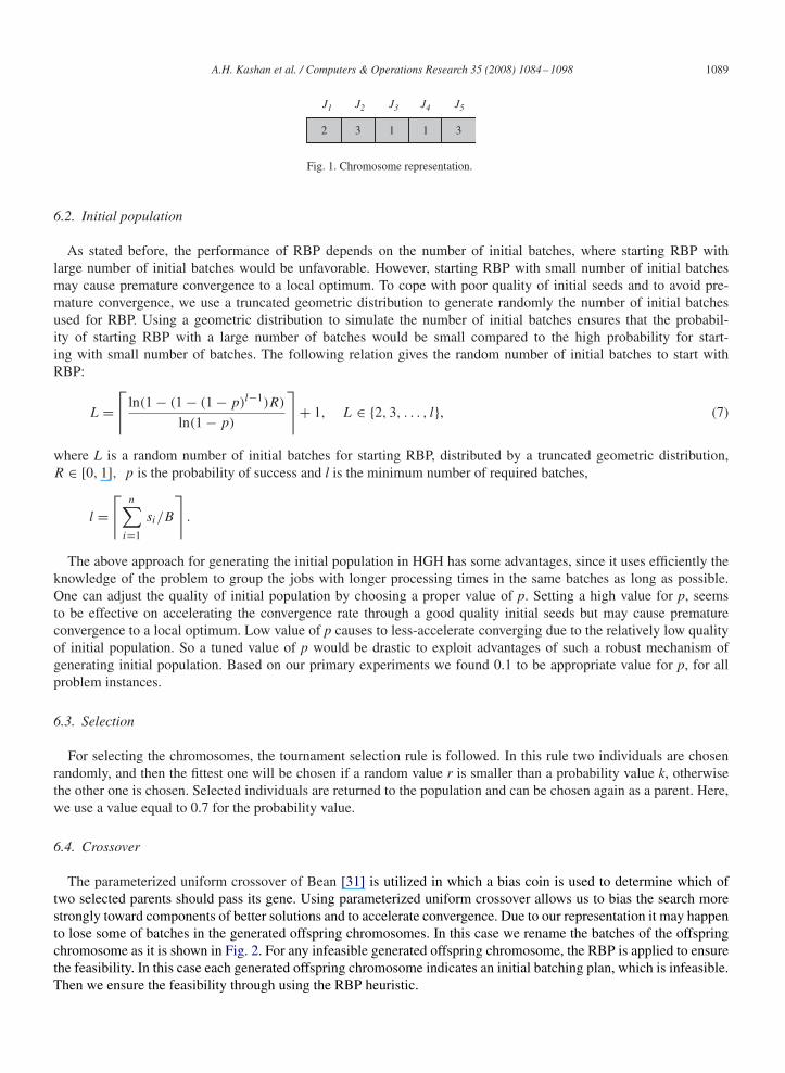
The parameterized uniform crossover of Bean [31] is utilized in which a bias coin is used to determine which oftwo selected parents should pass its gene. Using parameterized uniform crossover allows us to bias the search morestrongly toward components of better solutions and to accelerate convergence. Due to our representation it may happento lose some of batches in the generated offspring chromosomes. In this case we rename the batches of the offspringchromosome as it is shown in Fig. 2. For any infeasible generated offspring chromosome, the RBP is applied to ensurethe feasibility. In this case each generated offspring chromosome indicates an initial batching plan, which is infeasible.Then we ensure the feasibility through using the RBP heuristic.

1090 A.H. Kashan et al. / Computers & Operations Research 35 (2008) 1084–1098

J1 J2 J3 J4 J5

J1 J2 J3 J4 J5

3 1 3 2 1

Rename

1 4 2 3 4

T HH T H

Parent 1

Offspring

Parent 2

3 4 2 2 4 2 3 1 1 3

Fig. 2. Crossover procedure.

J1 J2 J3 J4 J5J1 J2 J3 J4 J5

SwapMutation

Offspring1 4 2 3 4 1 3 2 4 4Parent

Fig. 3. Mutation procedure.

6.5. Mutation

The swapping mutation is used as mutation operator. It selects two random genes of a selected chromosome andswaps their content. The feasibility of the mutated schedule is kept through using the RBP heuristic. Fig. 3 shows theswap mutation procedure applied for HGH.

6.6. Local search heuristics

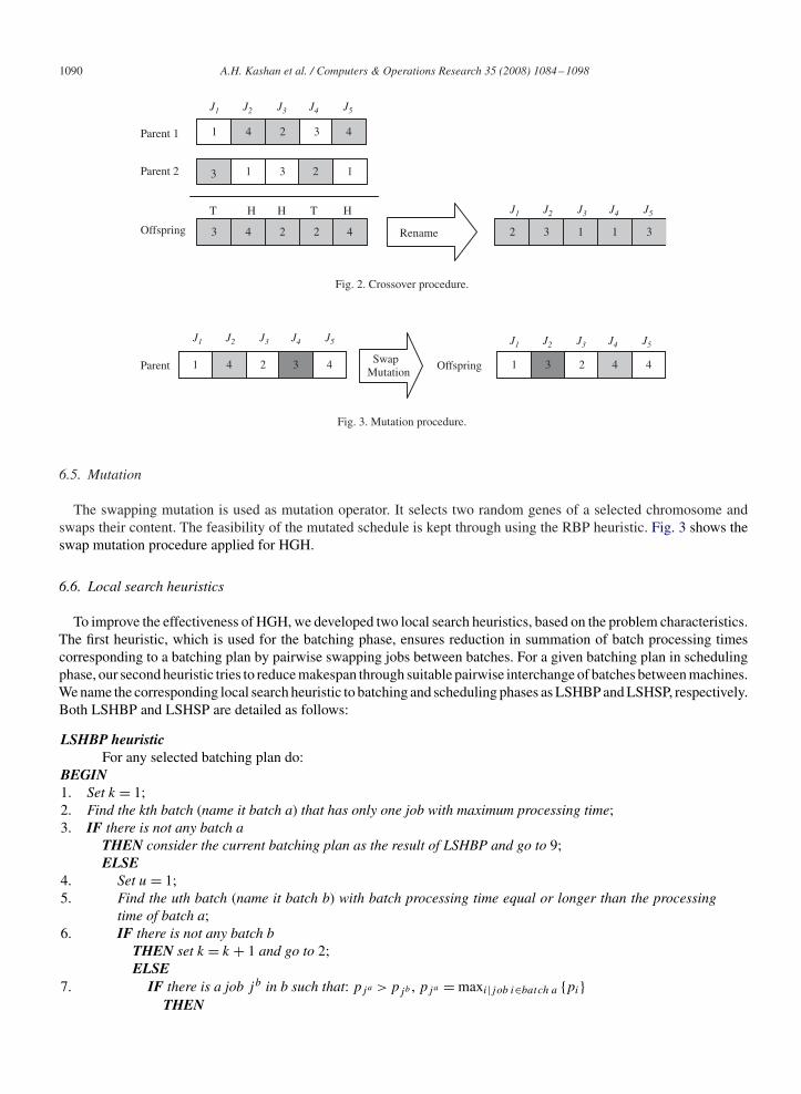
To improve the effectiveness of HGH, we developed two local search heuristics, based on the problem characteristics.The first heuristic, which is used for the batching phase, ensures reduction in summation of batch processing timescorresponding to a batching plan by pairwise swapping jobs between batches. For a given batching plan in schedulingphase, our second heuristic tries to reduce makespan through suitable pairwise interchange of batches between machines.We name the corresponding local search heuristic to batching and scheduling phases as LSHBP and LSHSP, respectively.Both LSHBP and LSHSP are detailed as follows:

LSHBP heuristicFor any selected batching plan do:

BEGIN1. Set k = 1;2. Find the kth batch (name it batch a) that has only one job with maximum processing time;3. IF there is not any batch a

THEN consider the current batching plan as the result of LSHBP and go to 9;ELSE

4. Set u = 1;5. Find the uth batch (name it batch b) with batch processing time equal or longer than the processing

time of batch a;6. IF there is not any batch b

THEN set k = k + 1 and go to 2;ELSE

7. IF there is a job jb in b such that: pja > pjb , pja = maxi|job i∈batch a {pi}THEN

A.H. Kashan et al. / Computers & Operations Research 35 (2008) 1084–1098 1091

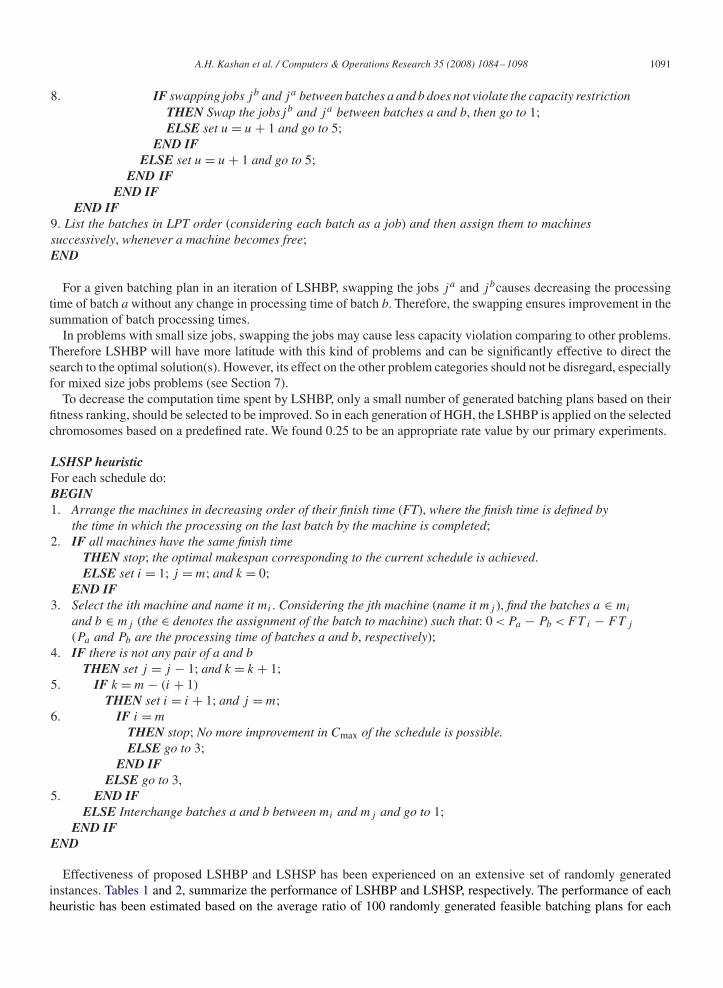
8. IF swapping jobs jb and ja between batches a and b does not violate the capacity restrictionTHEN Swap the jobsjb and ja between batches a and b, then go to 1;ELSE set u = u + 1 and go to 5;

END IFELSE set u = u + 1 and go to 5;

END IFEND IF

END IF9. List the batches in LPT order (considering each batch as a job) and then assign them to machinessuccessively, whenever a machine becomes free;END

For a given batching plan in an iteration of LSHBP, swapping the jobs ja and jbcauses decreasing the processingtime of batch a without any change in processing time of batch b. Therefore, the swapping ensures improvement in thesummation of batch processing times.

In problems with small size jobs, swapping the jobs may cause less capacity violation comparing to other problems.Therefore LSHBP will have more latitude with this kind of problems and can be significantly effective to direct thesearch to the optimal solution(s). However, its effect on the other problem categories should not be disregard, especiallyfor mixed size jobs problems (see Section 7).

To decrease the computation time spent by LSHBP, only a small number of generated batching plans based on theirfitness ranking, should be selected to be improved. So in each generation of HGH, the LSHBP is applied on the selectedchromosomes based on a predefined rate. We found 0.25 to be an appropriate rate value by our primary experiments.

LSHSP heuristicFor each schedule do:BEGIN1. Arrange the machines in decreasing order of their finish time (FT), where the finish time is defined by

the time in which the processing on the last batch by the machine is completed;2. IF all machines have the same finish time

THEN stop; the optimal makespan corresponding to the current schedule is achieved.ELSE set i = 1; j = m; and k = 0;

END IF3. Select the ith machine and name it mi . Considering the jth machine (name it mj ), find the batches a ∈ mi

and b ∈ mj (the ∈ denotes the assignment of the batch to machine) such that: 0 < Pa − Pb < FT i − FT j

(Pa and Pb are the processing time of batches a and b, respectively);4. IF there is not any pair of a and b

THEN set j = j − 1; and k = k + 1;5. IF k = m − (i + 1)

THEN set i = i + 1; and j = m;6. IF i = m

THEN stop; No more improvement in Cmax of the schedule is possible.ELSE go to 3;

END IFELSE go to 3,

5. END IFELSE Interchange batches a and b between mi and mj and go to 1;

END IFEND

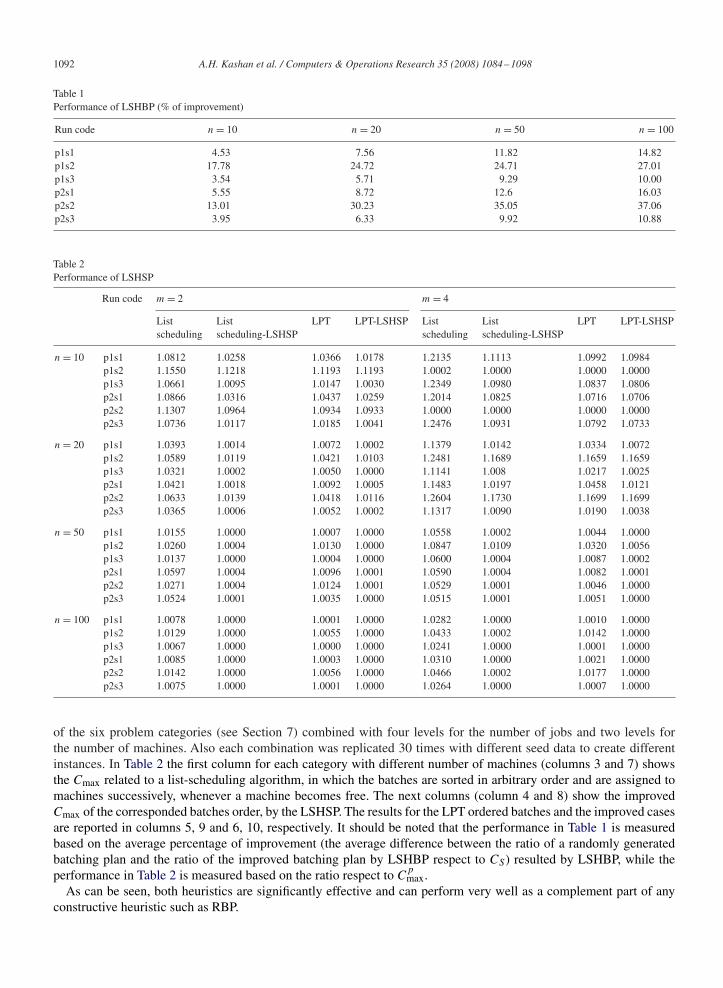
Effectiveness of proposed LSHBP and LSHSP has been experienced on an extensive set of randomly generatedinstances. Tables 1 and 2, summarize the performance of LSHBP and LSHSP, respectively. The performance of eachheuristic has been estimated based on the average ratio of 100 randomly generated feasible batching plans for each

1092 A.H. Kashan et al. / Computers & Operations Research 35 (2008) 1084–1098

Table 1Performance of LSHBP (% of improvement)

Run code n = 10 n = 20 n = 50 n = 100

p1s1 4.53 7.56 11.82 14.82p1s2 17.78 24.72 24.71 27.01p1s3 3.54 5.71 9.29 10.00p2s1 5.55 8.72 12.6 16.03p2s2 13.01 30.23 35.05 37.06p2s3 3.95 6.33 9.92 10.88

Table 2Performance of LSHSP

Run code m = 2 m = 4

List List LPT LPT-LSHSP List List LPT LPT-LSHSPscheduling scheduling-LSHSP scheduling scheduling-LSHSP

n = 10 p1s1 1.0812 1.0258 1.0366 1.0178 1.2135 1.1113 1.0992 1.0984p1s2 1.1550 1.1218 1.1193 1.1193 1.0002 1.0000 1.0000 1.0000p1s3 1.0661 1.0095 1.0147 1.0030 1.2349 1.0980 1.0837 1.0806p2s1 1.0866 1.0316 1.0437 1.0259 1.2014 1.0825 1.0716 1.0706p2s2 1.1307 1.0964 1.0934 1.0933 1.0000 1.0000 1.0000 1.0000p2s3 1.0736 1.0117 1.0185 1.0041 1.2476 1.0931 1.0792 1.0733

n = 20 p1s1 1.0393 1.0014 1.0072 1.0002 1.1379 1.0142 1.0334 1.0072p1s2 1.0589 1.0119 1.0421 1.0103 1.2481 1.1689 1.1659 1.1659p1s3 1.0321 1.0002 1.0050 1.0000 1.1141 1.008 1.0217 1.0025p2s1 1.0421 1.0018 1.0092 1.0005 1.1483 1.0197 1.0458 1.0121p2s2 1.0633 1.0139 1.0418 1.0116 1.2604 1.1730 1.1699 1.1699p2s3 1.0365 1.0006 1.0052 1.0002 1.1317 1.0090 1.0190 1.0038

n = 50 p1s1 1.0155 1.0000 1.0007 1.0000 1.0558 1.0002 1.0044 1.0000p1s2 1.0260 1.0004 1.0130 1.0000 1.0847 1.0109 1.0320 1.0056p1s3 1.0137 1.0000 1.0004 1.0000 1.0600 1.0004 1.0087 1.0002p2s1 1.0597 1.0004 1.0096 1.0001 1.0590 1.0004 1.0082 1.0001p2s2 1.0271 1.0004 1.0124 1.0001 1.0529 1.0001 1.0046 1.0000p2s3 1.0524 1.0001 1.0035 1.0000 1.0515 1.0001 1.0051 1.0000

n = 100 p1s1 1.0078 1.0000 1.0001 1.0000 1.0282 1.0000 1.0010 1.0000p1s2 1.0129 1.0000 1.0055 1.0000 1.0433 1.0002 1.0142 1.0000p1s3 1.0067 1.0000 1.0000 1.0000 1.0241 1.0000 1.0001 1.0000p2s1 1.0085 1.0000 1.0003 1.0000 1.0310 1.0000 1.0021 1.0000p2s2 1.0142 1.0000 1.0056 1.0000 1.0466 1.0002 1.0177 1.0000p2s3 1.0075 1.0000 1.0001 1.0000 1.0264 1.0000 1.0007 1.0000

of the six problem categories (see Section 7) combined with four levels for the number of jobs and two levels forthe number of machines. Also each combination was replicated 30 times with different seed data to create differentinstances. In Table 2 the first column for each category with different number of machines (columns 3 and 7) showsthe Cmax related to a list-scheduling algorithm, in which the batches are sorted in arbitrary order and are assigned tomachines successively, whenever a machine becomes free. The next columns (column 4 and 8) show the improvedCmax of the corresponded batches order, by the LSHSP. The results for the LPT ordered batches and the improved casesare reported in columns 5, 9 and 6, 10, respectively. It should be noted that the performance in Table 1 is measuredbased on the average percentage of improvement (the average difference between the ratio of a randomly generatedbatching plan and the ratio of the improved batching plan by LSHBP respect to CS) resulted by LSHBP, while theperformance in Table 2 is measured based on the ratio respect to C

pmax.

As can be seen, both heuristics are significantly effective and can perform very well as a complement part of anyconstructive heuristic such as RBP.

A.H. Kashan et al. / Computers & Operations Research 35 (2008) 1084–1098 1093

In each generation of HGH, the new population is formed by the offspring generated by GA operators. The rest ofthe population is filled with the best chromosomes of the former generation.

6.7. Parameter tuning

For each GA there are a number of parameters which choosing a proper value for them affects the search behavior andimproves the quality of convergence. These parameters include the population size, number of generations, crossoverrate, mutation rate and the head probability of the bias coin. For tuning crossover rate, mutation rate and the headprobability, different values are considered; 0.5 and 0.7 for crossover rate, 0.05, 0.1 and 0.15 for mutation rate and0.7 and 0.9 for head probability. Based on the primary experiments on HGH, the appropriate values found to be 0.5,0.15 and 0.9 for crossover rate, mutation rate and the head probability, respectively. About the population size andstopping criteria, we evaluated the pairs (n, 50) and (2n, 100), where the first member of these ordered pairs denotesthe population size (which increases by the problem size) and the second one indicates the number of generations.The results for the pair of (2n, 100) are slightly better in average performance (while there is not any difference inthe best and the worst-case performance) at the expense of significant increase in running times. So, it is preferred tokeep the pair (n, 50) to provide good results together with saving of the execution time. However the HGH will bestopped if there is no improvement in the best solution obtained in last 15 generations. Worth to mention that to avoiduseless computations in both HGH and SA, we set an extra stopping criterion that is getting to the lower bound solutionexplained in Section 4.

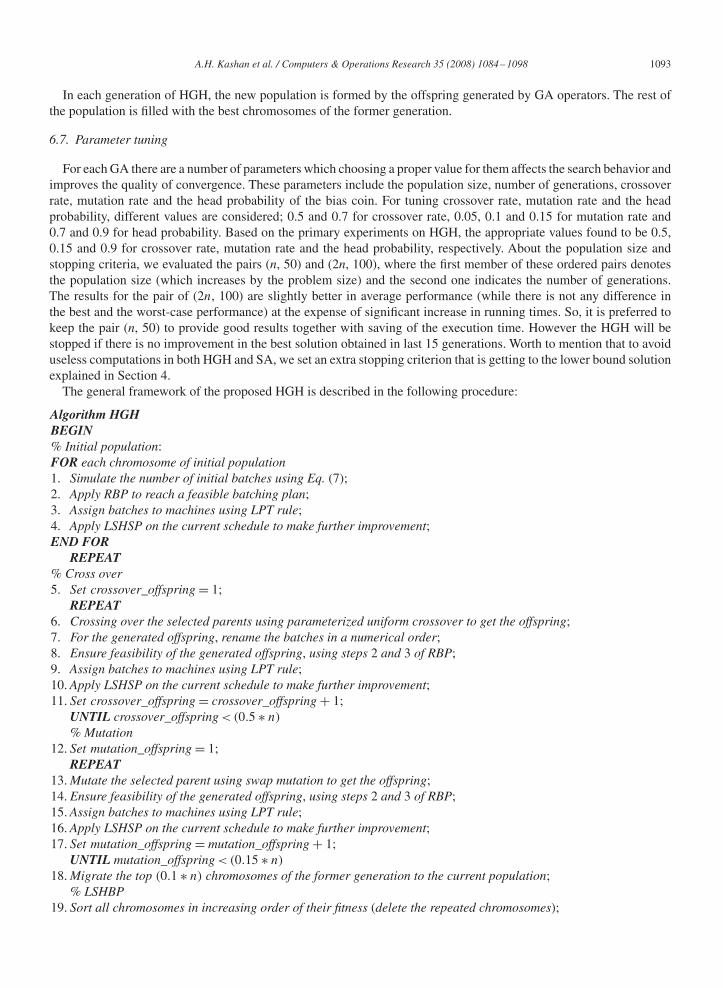
The general framework of the proposed HGH is described in the following procedure:

Algorithm HGHBEGIN% Initial population:FOR each chromosome of initial population1. Simulate the number of initial batches using Eq. (7);2. Apply RBP to reach a feasible batching plan;3. Assign batches to machines using LPT rule;4. Apply LSHSP on the current schedule to make further improvement;END FOR

REPEAT% Cross over5. Set crossover_offspring = 1;

REPEAT6. Crossing over the selected parents using parameterized uniform crossover to get the offspring;7. For the generated offspring, rename the batches in a numerical order;8. Ensure feasibility of the generated offspring, using steps 2 and 3 of RBP;9. Assign batches to machines using LPT rule;10. Apply LSHSP on the current schedule to make further improvement;11. Set crossover_offspring = crossover_offspring + 1;

UNTIL crossover_offspring < (0.5 ∗ n)

% Mutation12. Set mutation_offspring = 1;

REPEAT13. Mutate the selected parent using swap mutation to get the offspring;14. Ensure feasibility of the generated offspring, using steps 2 and 3 of RBP;15. Assign batches to machines using LPT rule;16. Apply LSHSP on the current schedule to make further improvement;17. Set mutation_offspring = mutation_offspring + 1;

UNTIL mutation_offspring < (0.15 ∗ n)

18. Migrate the top (0.1 ∗ n) chromosomes of the former generation to the current population;% LSHBP

19. Sort all chromosomes in increasing order of their fitness (delete the repeated chromosomes);

1094 A.H. Kashan et al. / Computers & Operations Research 35 (2008) 1084–1098

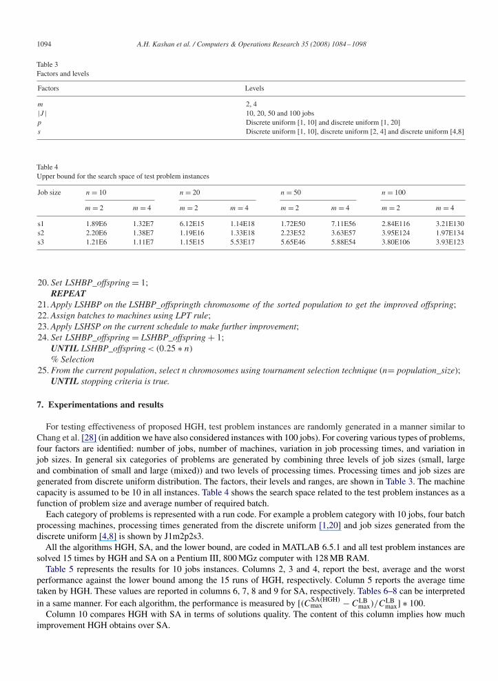
Table 3Factors and levels

Factors Levels

m 2, 4|J | 10, 20, 50 and 100 jobsp Discrete uniform [1, 10] and discrete uniform [1, 20]s Discrete uniform [1, 10], discrete uniform [2, 4] and discrete uniform [4,8]

Table 4Upper bound for the search space of test problem instances

Job size n = 10 n = 20 n = 50 n = 100

m = 2 m = 4 m = 2 m = 4 m = 2 m = 4 m = 2 m = 4

s1 1.89E6 1.32E7 6.12E15 1.14E18 1.72E50 7.11E56 2.84E116 3.21E130s2 2.20E6 1.38E7 1.19E16 1.33E18 2.23E52 3.63E57 3.95E124 1.97E134s3 1.21E6 1.11E7 1.15E15 5.53E17 5.65E46 5.88E54 3.80E106 3.93E123

20. Set LSHBP_offspring = 1;REPEAT

21. Apply LSHBP on the LSHBP_offspringth chromosome of the sorted population to get the improved offspring;22. Assign batches to machines using LPT rule;23. Apply LSHSP on the current schedule to make further improvement;24. Set LSHBP_offspring = LSHBP_offspring + 1;

UNTIL LSHBP_offspring < (0.25 ∗ n)

% Selection25. From the current population, select n chromosomes using tournament selection technique (n= population_size);

UNTIL stopping criteria is true.

7. Experimentations and results

For testing effectiveness of proposed HGH, test problem instances are randomly generated in a manner similar toChang et al. [28] (in addition we have also considered instances with 100 jobs). For covering various types of problems,four factors are identified: number of jobs, number of machines, variation in job processing times, and variation injob sizes. In general six categories of problems are generated by combining three levels of job sizes (small, largeand combination of small and large (mixed)) and two levels of processing times. Processing times and job sizes aregenerated from discrete uniform distribution. The factors, their levels and ranges, are shown in Table 3. The machinecapacity is assumed to be 10 in all instances. Table 4 shows the search space related to the test problem instances as afunction of problem size and average number of required batch.

Each category of problems is represented with a run code. For example a problem category with 10 jobs, four batchprocessing machines, processing times generated from the discrete uniform [1,20] and job sizes generated from thediscrete uniform [4,8] is shown by J1m2p2s3.

All the algorithms HGH, SA, and the lower bound, are coded in MATLAB 6.5.1 and all test problem instances aresolved 15 times by HGH and SA on a Pentium III, 800 MGz computer with 128 MB RAM.

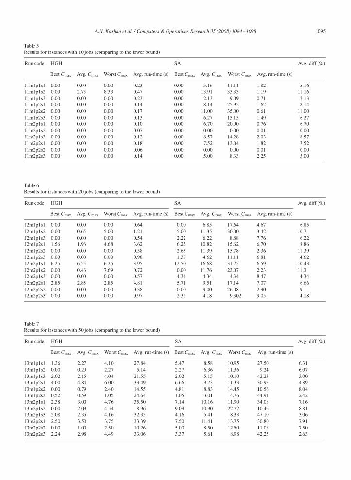
Table 5 represents the results for 10 jobs instances. Columns 2, 3 and 4, report the best, average and the worstperformance against the lower bound among the 15 runs of HGH, respectively. Column 5 reports the average timetaken by HGH. These values are reported in columns 6, 7, 8 and 9 for SA, respectively. Tables 6–8 can be interpretedin a same manner. For each algorithm, the performance is measured by [(CSA(HGH)

max − CLBmax)/CLB

max] ∗ 100.Column 10 compares HGH with SA in terms of solutions quality. The content of this column implies how much

improvement HGH obtains over SA.

A.H. Kashan et al. / Computers & Operations Research 35 (2008) 1084–1098 1095

Table 5Results for instances with 10 jobs (comparing to the lower bound)

Run code HGH SA Avg. diff (%)

Best Cmax Avg. Cmax Worst Cmax Avg. run-time (s) Best Cmax Avg. Cmax Worst Cmax Avg. run-time (s)

J1m1p1s1 0.00 0.00 0.00 0.23 0.00 5.16 11.11 1.82 5.16J1m1p1s2 0.00 2.75 8.33 0.47 0.00 13.91 33.33 1.19 11.16J1m1p1s3 0.00 0.00 0.00 0.23 0.00 2.13 9.09 0.71 2.13J1m1p2s1 0.00 0.00 0.00 0.14 0.00 8.14 25.92 1.62 8.14J1m1p2s2 0.00 0.00 0.00 0.17 0.00 11.00 35.00 0.61 11.00J1m1p2s3 0.00 0.00 0.00 0.13 0.00 6.27 15.15 1.49 6.27J1m2p1s1 0.00 0.00 0.00 0.10 0.00 6.70 20.00 0.76 6.70J1m2p1s2 0.00 0.00 0.00 0.07 0.00 0.00 0.00 0.01 0.00J1m2p1s3 0.00 0.00 0.00 0.12 0.00 8.57 14.28 2.03 8.57J1m2p2s1 0.00 0.00 0.00 0.18 0.00 7.52 13.04 1.82 7.52J1m2p2s2 0.00 0.00 0.00 0.06 0.00 0.00 0.00 0.01 0.00J1m2p2s3 0.00 0.00 0.00 0.14 0.00 5.00 8.33 2.25 5.00

Table 6Results for instances with 20 jobs (comparing to the lower bound)

Run code HGH SA Avg. diff (%)

Best Cmax Avg. Cmax Worst Cmax Avg. run-time (s) Best Cmax Avg. Cmax Worst Cmax Avg. run-time (s)

J2m1p1s1 0.00 0.00 0.00 0.64 0.00 6.85 17.64 4.67 6.85J2m1p1s2 0.00 0.65 5.00 1.21 5.00 11.35 30.00 3.42 10.7J2m1p1s3 0.00 0.00 0.00 0.54 2.22 6.22 8.88 7.76 6.22J2m1p2s1 1.56 1.96 4.68 3.62 6.25 10.82 15.62 6.70 8.86J2m1p2s2 0.00 0.00 0.00 0.58 2.63 11.39 15.78 2.36 11.39J2m1p2s3 0.00 0.00 0.00 0.98 1.38 4.62 11.11 6.81 4.62J2m2p1s1 6.25 6.25 6.25 3.95 12.50 16.68 31.25 6.59 10.43J2m2p1s2 0.00 0.46 7.69 0.72 0.00 11.76 23.07 2.23 11.3J2m2p1s3 0.00 0.00 0.00 0.57 4.34 4.34 4.34 8.47 4.34J2m2p2s1 2.85 2.85 2.85 4.81 5.71 9.51 17.14 7.07 6.66J2m2p2s2 0.00 0.00 0.00 0.38 0.00 9.00 26.08 2.90 9J2m2p2s3 0.00 0.00 0.00 0.97 2.32 4.18 9.302 9.05 4.18

Table 7Results for instances with 50 jobs (comparing to the lower bound)

Run code HGH SA Avg. diff (%)

Best Cmax Avg. Cmax Worst Cmax Avg. run-time (s) Best Cmax Avg. Cmax Worst Cmax Avg. run-time (s)

J3m1p1s1 1.36 2.27 4.10 27.84 5.47 8.58 10.95 27.50 6.31J3m1p1s2 0.00 0.29 2.27 5.14 2.27 6.36 11.36 9.24 6.07J3m1p1s3 2.02 2.15 4.04 21.55 2.02 5.15 10.10 42.23 3.00J3m1p2s1 4.00 4.84 6.00 33.49 6.66 9.73 11.33 30.95 4.89J3m1p2s2 0.00 0.79 2.40 14.55 4.81 8.83 14.45 10.56 8.04J3m1p2s3 0.52 0.59 1.05 24.64 1.05 3.01 4.76 44.91 2.42J3m2p1s1 2.38 3.00 4.76 35.50 7.14 10.16 11.90 34.08 7.16J3m2p1s2 0.00 2.09 4.54 8.96 9.09 10.90 22.72 10.46 8.81J3m2p1s3 2.08 2.35 4.16 32.35 4.16 5.41 8.33 47.10 3.06J3m2p2s1 2.50 3.50 3.75 33.39 7.50 11.41 13.75 30.80 7.91J3m2p2s2 0.00 1.00 2.50 10.26 5.00 8.50 12.50 11.08 7.50J3m2p2s3 2.24 2.98 4.49 33.06 3.37 5.61 8.98 42.25 2.63

1096 A.H. Kashan et al. / Computers & Operations Research 35 (2008) 1084–1098

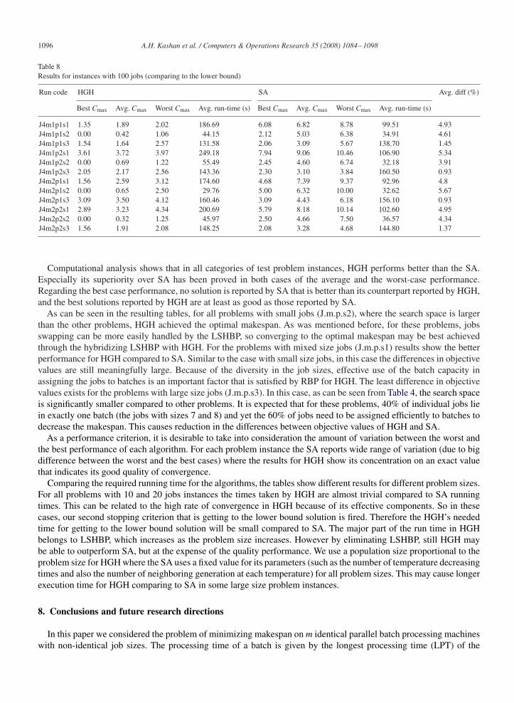
Table 8Results for instances with 100 jobs (comparing to the lower bound)

Run code HGH SA Avg. diff (%)

Best Cmax Avg. Cmax Worst Cmax Avg. run-time (s) Best Cmax Avg. Cmax Worst Cmax Avg. run-time (s)

J4m1p1s1 1.35 1.89 2.02 186.69 6.08 6.82 8.78 99.51 4.93J4m1p1s2 0.00 0.42 1.06 44.15 2.12 5.03 6.38 34.91 4.61J4m1p1s3 1.54 1.64 2.57 131.58 2.06 3.09 5.67 138.70 1.45J4m1p2s1 3.61 3.72 3.97 249.18 7.94 9.06 10.46 106.90 5.34J4m1p2s2 0.00 0.69 1.22 55.49 2.45 4.60 6.74 32.18 3.91J4m1p2s3 2.05 2.17 2.56 143.36 2.30 3.10 3.84 160.50 0.93J4m2p1s1 1.56 2.59 3.12 174.60 4.68 7.39 9.37 92.96 4.8J4m2p1s2 0.00 0.65 2.50 29.76 5.00 6.32 10.00 32.62 5.67J4m2p1s3 3.09 3.50 4.12 160.46 3.09 4.43 6.18 156.10 0.93J4m2p2s1 2.89 3.23 4.34 200.69 5.79 8.18 10.14 102.60 4.95J4m2p2s2 0.00 0.32 1.25 45.97 2.50 4.66 7.50 36.57 4.34J4m2p2s3 1.56 1.91 2.08 148.25 2.08 3.28 4.68 144.80 1.37

Computational analysis shows that in all categories of test problem instances, HGH performs better than the SA.Especially its superiority over SA has been proved in both cases of the average and the worst-case performance.Regarding the best case performance, no solution is reported by SA that is better than its counterpart reported by HGH,and the best solutions reported by HGH are at least as good as those reported by SA.

As can be seen in the resulting tables, for all problems with small jobs (J.m.p.s2), where the search space is largerthan the other problems, HGH achieved the optimal makespan. As was mentioned before, for these problems, jobsswapping can be more easily handled by the LSHBP, so converging to the optimal makespan may be best achievedthrough the hybridizing LSHBP with HGH. For the problems with mixed size jobs (J.m.p.s1) results show the betterperformance for HGH compared to SA. Similar to the case with small size jobs, in this case the differences in objectivevalues are still meaningfully large. Because of the diversity in the job sizes, effective use of the batch capacity inassigning the jobs to batches is an important factor that is satisfied by RBP for HGH. The least difference in objectivevalues exists for the problems with large size jobs (J.m.p.s3). In this case, as can be seen from Table 4, the search spaceis significantly smaller compared to other problems. It is expected that for these problems, 40% of individual jobs liein exactly one batch (the jobs with sizes 7 and 8) and yet the 60% of jobs need to be assigned efficiently to batches todecrease the makespan. This causes reduction in the differences between objective values of HGH and SA.

As a performance criterion, it is desirable to take into consideration the amount of variation between the worst andthe best performance of each algorithm. For each problem instance the SA reports wide range of variation (due to bigdifference between the worst and the best cases) where the results for HGH show its concentration on an exact valuethat indicates its good quality of convergence.

Comparing the required running time for the algorithms, the tables show different results for different problem sizes.For all problems with 10 and 20 jobs instances the times taken by HGH are almost trivial compared to SA runningtimes. This can be related to the high rate of convergence in HGH because of its effective components. So in thesecases, our second stopping criterion that is getting to the lower bound solution is fired. Therefore the HGH’s neededtime for getting to the lower bound solution will be small compared to SA. The major part of the run time in HGHbelongs to LSHBP, which increases as the problem size increases. However by eliminating LSHBP, still HGH maybe able to outperform SA, but at the expense of the quality performance. We use a population size proportional to theproblem size for HGH where the SA uses a fixed value for its parameters (such as the number of temperature decreasingtimes and also the number of neighboring generation at each temperature) for all problem sizes. This may cause longerexecution time for HGH comparing to SA in some large size problem instances.

8. Conclusions and future research directions

In this paper we considered the problem of minimizing makespan on m identical parallel batch processing machineswith non-identical job sizes. The processing time of a batch is given by the longest processing time (LPT) of the

A.H. Kashan et al. / Computers & Operations Research 35 (2008) 1084–1098 1097

jobs in the batch. To examine the problem search space, we developed an enumerative formula as a function of bothproblem size (n) and the least number of required batches (l). We proposed a hybrid genetic heuristic (HGH) based ona batch-based representation. Our computational results show that the HGH outperforms a simulated annealing (SA)approach, taken from the literature as a comparator algorithm. Also its good performance comparing to a developedlower bound is indicated.

Some characteristics such as using a robust mechanism for generating initial population, using an efficient localsearch heuristic (LSHBP) to bring longer jobs together as a batch, which has the ability of steering quickly the searchtoward the optimal solution(s) and using a local search heuristic (LSHSP) to further improve machines load, are thecases that cause HGH to dominate the SA approach.

For future research, the extension of our approach could include due date related performance measures and alsoconsidering dynamic job arrivals and incompatible families.

References

[1] Lee C-Y, Uzsoy R, Martin-Vega L-A. Efficient algorithms for scheduling semiconductor burn-in operations. Operations Research 1992;40:764–75.

[2] Ikura Y, Gimple M. Efficient scheduling algorithms for a single batch processing machine. Operations Research Letters 1986;5:61–5.[3] Li C-L, Lee C-Y. Scheduling with agreeable release times and due dates on a batch processing machine. European Journal of Operational

Research 1997;96:564–9.[4] Brucker P, Gladky A, Hoogeveen H, Kovalyov M-Y, Potts C, Tautenhahn T. et al. Scheduling a batching machine. Journal of Scheduling

1998;1:31–54.[5] Chandru V, Lee C-Y, Uzsoy R. Minimizing total completion time on batch processing machines. International Journal of Production Research

1993;31:2097–121.[6] Dupont L, Jolai Ghazvini F. Branch and bound method for minimizing mean flow time on a single batch processing machine. International

Journal of Industrial Engineering: Applications and Practice 1997;4:197–203.[7] Uzsoy R, Yang Y. Minimizing total weighted completion time on a single batch processing machine. Production and Operations Management

1997;6:57–73.[8] Lee C-Y, Uzsoy R. Minimizing makespan on a single batch processing machine with dynamic job arrivals. International Journal of Production

Research 1999;37:219–36.[9] Kempf K-G, Uzsoy R, Wang C-S. Scheduling a single batch processing machine with secondary resource constraints. Journal of Manufacturing

Systems 1998;17:37–51.[10] Uzsoy R. Scheduling batch processing machines with incompatible job families. International Journal of Production Research 1995;33:

2685–708.[11] Mehta S-V, Uzsoy R. Minimizing total tardiness on a batch processing machine with incompatible job families. IIE Transactions 1998;30:

165–78.[12] Dobson G, Nambimadom R-S. The batch loading and scheduling problem. Research Report, Simon School of Business Administration,

University of Rochester, Rochester, NY, USA; 1992.[13] Jolai F. Minimizing number of tardy jobs on a batch processing machine with incompatible job families. European Journal of Operational

Research 2005;162:184–90.[14] Chandru V, Lee C-Y, Uzsoy R. Minimizing total completion time on a batch processing machine with job families. Operations Research Letters

1993;13:61–5.[15] Hochbaum D-S, Landy D. Algorithms and heuristics for scheduling semiconductor burn-in operations. Research Report ESRC 94-8, University

of California, Berkeley, USA; 1994.[16] Uzsoy R. A single batch processing machine with non-identical job sizes. International Journal of Production Research 1994;32:1615–35.[17] Jolai Ghazvini F, Dupont L. Minimizing mean flow time on a single batch processing machine with non-identical job sizes. International Journal

of Production Economics 1998;55:273–80.[18] Dupont L, Dhaenens-Flipo C. Minimizing the makespan on a batch machine with non-identical job sizes: an exact procedure. Computers and

Operations Research 2002;29:807–19.[19] Shuguang L, Guojun L, Xiaoli W, Qiming L. Minimizing makespan on a single batching machine with release times and non-identical job

sizes. Operations Research Letters 2005;33:157–64.[20] Wang C, Uzsoy R. A genetic algorithm to minimize maximum lateness on a batch processing machine. Computers and Operations Research

2002;29:1621–40.[21] Melouk S, Damodaran P, Chang P-Y. Minimizing make span for single machine batch processing with non-identical job sizes using simulated

annealing. International Journal of Production Economics 2004;87:141–7.[22] Koh S-G, Koo P-H, Kim D-C, Hur W-S. Scheduling a single batch processing machine with arbitrary job sizes and incompatible job families.

International Journal of Production Economics 2005;98:81–96.[23] Graham R-L. Bounds on multiprocessor timing anomalies. SIAM Journal of Applied Mathematics 1969;17:416–29.[24] Balasubramanian H, Monch L, Fowler J, Pfund M. Genetic algorithm based scheduling of parallel batch machines with incompatible job

families to minimize total weighted tardiness. International Journal of Production Research 2004;42:1621–38.

1098 A.H. Kashan et al. / Computers & Operations Research 35 (2008) 1084–1098

[25] Monch L, Balasubramanian H, Fowler J, Pfund M. Heuristic scheduling of jobs on parallel batch machines with incompatible job families andunequal ready times. Computers and Operations Research 2005;32:2731–50.

[26] Koh S-G, Koo P-H, Ha J-W, Lee W-S. Scheduling parallel batch processing machines with arbitrary job sizes and incompatible job families.International Journal of Production Research 2004;42:4091–107.

[27] Malve S, Uzsoy R. A genetic algorithm for minimizing maximum lateness on parallel identical batch processing machines with dynamic jobarrivals and incompatible job families. Computers and Operations Research, 2005, in press.

[28] Chang P-Y, Damodaran P, Melouk S. Minimizing makespan on parallel batch processing machines. International Journal of Production Research2004;42:4211–20.

[29] McNaughton R. Scheduling with deadlines and loss functions. Management Science 1959;6:1–12.[30] Gen M, Cheng R. Genetic algorithms and engineering design. New York: Wiley; 1997.[31] Bean J-C. Genetic algorithms and random keys for sequencing and optimization. ORSA Journal of Computing 1994;6:154–60.