a customized gabor filter for unsupervised color image segmentation

Image and Vision Computing 27 (2009) 489–501

Contents lists available at ScienceDirect

Image and Vision Computing

journal homepage: www.elsevier .com/locate / imavis

A customized Gabor filter for unsupervised color image segmentation

Jesmin F. Khan *, Reza R. Adhami, Sharif M.A. BhuiyanDepartment of Electrical and Computer Engineering, University of Alabama in Huntsville, 272 Engineering Building, Huntsville, AL 35899, USA

a r t i c l e i n f o

Article history:Received 4 November 2007Received in revised form 18 April 2008Accepted 3 July 2008

Keywords:Unsupervised clusteringExpectation maximizationImage segmentationSchwarz criterionGabor filter

0262-8856/$ - see front matter � 2008 Elsevier B.V. Adoi:10.1016/j.imavis.2008.07.001

* Corresponding author. Tel.: +1 256 824 6316; faxE-mail addresses: [email protected], [email protected]

ece.uah.edu (R.R. Adhami), [email protected] (S.M

a b s t r a c t

This paper presents work on accurate image segmentation utilizing local image characteristics. Imagefeatures are measured by employing an appropriate Gabor filter with adaptively chosen size, orientation,frequency and phase for each pixel. An image property called phase divergence is used for the selection ofthe appropriate filter size. Characteristic features related to the change in brightness, color, texture andposition are extracted for each pixel at the selected size of the filter. In order to cluster the pixels intodifferent regions, the joint distribution of these pixel features is modeled by a mixture of Gaussians uti-lizing three variants of the expectation maximization (EM) algorithm. The three different versions of EMused in this work for unsupervised clustering are: (1) penalized EM, (2) penalized stochastic EM, and (3)penalized inverse EM. Given the desired number of Gaussian mixture components, all three EM algo-rithms estimate the parameters of the mixture of Gaussians model that represents the joint distributionof pixel features. We determine the value of the number of models that best suits the natural number ofclusters present in the image based on the Schwarz criterion, which maximizes the posterior probabilityof the number of groups given the samples of observation. This segmentation algorithm has been testedon the images of the Berkeley segmentation benchmark and the performance has demonstrated the effec-tiveness, accuracy and superiority of the proposed method.

� 2008 Elsevier B.V. All rights reserved.

1. Introduction

Image segmentation is an essential task for image analysis andpattern recognition. It is the procedure of dividing an image into itsconstituent regions, where the regions generally correspond toobjects or parts of objects. There are a wide variety of methodsin the literature for image segmentation. However, inaccurate par-titioning of an image is inevitable in most segmentation algo-rithms. In this paper, we have developed a color imagesegmentation algorithm that is good enough to yield improved im-age segmentation, so that each region is consistent and there is nounion of any two inhomogeneous regions.

Color is a powerful descriptor and humans can discern thou-sands of color shades and intensities compared to about only twodozen shades of gray. This factor is important in many pattern rec-ognition and image processing applications. The additional infor-mation provided by color often simplifies the image analysisprocess and yields better results than methods using only grayscale information. Due to increasing demand, more research hasrecently focused on color image segmentation. Approaches for col-or image segmentation can be categorized as: edge detection; sta-tistical approach; histogram thresholding; region based methods

ll rights reserved.

: +1 256 824 6803.ah.edu (J.F. Khan), adhami@

.A. Bhuiyan).

such as thresholding, region growing, region splitting, and merg-ing; color perception model; characteristic feature clustering; neu-ral network; physics based technique and fuzzy set theory [1,2].

Histogram thresholding is the most widely used technique formonochrome image segmentation [3]. For color images, multiplehistogram based thresholding divides color space by thresholdingeach color component histogram. But representing the histogramof a color image in a three-dimension (3D) array and selectingthresholds in this histogram is not a trivial job [4]. To solve thisproblem, several efficient methods are developed for storing andprocessing the information of the image in a 3D color space [5–7]. A hierarchical approach in the homogeneity domain is studied[8] for color image segmentation. Clustering of characteristic fea-tures applied to image segmentation is the multidimensionalextension of the concept of thresholding [9]. A set of effective colorfeatures extracted for image segmentation have been proposed in[10–12]. In [10], Karhunen–Loeve transformation is applied toRGB color space to extract a set of effective color features withlarge discriminant power in order to isolate the clusters in a givenregion. The same idea is used in [11] to extract the principal com-ponents of a color distribution for detecting clusters. A methodbased on K-nearest neighbor technique is proposed in [12] fordetecting fruit and leaves in a color scene. The feature vectorsare based on the YUV color space.

In [13] a color image segmentation algorithm based on a newform of contrast information and CIE L*a*b* color space, is

mailto:[email protected]


mailto:adhami@ ece.uah.edu

mailto:adhami@ ece.uah.edu


http://www.sciencedirect.com/science/journal/02628856

http://www.elsevier.com/locate/imavis

490 J.F. Khan et al. / Image and Vision Computing 27 (2009) 489–501

proposed. A multiresolution color image segmentation (MCIS)algorithm that uses Markov random fields (MRF’s) is presented in[14]. This approach is a relaxation process that converges to themaximum a posteriori (MAP) estimate of the segmentation. Therival penalization controlled competitive learning (RPCCL) algo-rithm is applied to perform unsupervised data clustering and colorimage segmentation in [15]. After generating a multiscale repre-sentation of the image information using non-parametric cluster-ing, a graph theoretic algorithm is used to synthesize regions andproduce the final segmentation results in [16]. The basic idea forunsupervised color image segmentation in [17] is to apply meanshift clustering to obtain an over-segmentation, and then mergeregions at multiple scales to minimize the minimum descriptionlength (MDL) criterion. Feature space and spatial information arecombined in [18] by using an inter-region dissimilarity relationto segment a color image.

In this paper we use multiple features clustering to performimage segmentation, where we take into account both characteris-tic features and the spatial relation between pixels simultaneously.The characteristic features are considered as a local neighborhoodproperty. Therefore, in order for those features to be useful theymust be computed in a neighborhood, which requires the determi-nation of the appropriate size of the window that defines the localstructure. This requirement is the same as the problem of scaleselection. In this paper we propose a novel method of scale selec-tion which is based on a newly introduced local image propertycalled phase divergence. Our approach for image segmentation in-volves clustering the pixels into regions by modeling the joint dis-tribution of pixel brightness, color, texture and position featureswith a mixture of Gaussians employing three variants of the EMalgorithm: penalized EM (PEM), penalized stochastic EM (PSEM)and penalized inverse EM (PIEM). PEM and PSEM are proposed in[19], and in this paper we have applied those algorithms for imagesegmentation purposes. Furthermore, we introduce and investi-

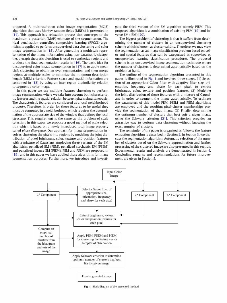
Fig. 1. Block diagram of th

gate the third variant of the EM algorithm namely PIEM. Thisproposed algorithm is a combination of existing PEM [19] and in-verse EM (IEM) [20].

The biggest problem of clustering is that it suffers from deter-mining the number of clusters in an unsupervised clusteringscheme which is known as cluster validity. Therefore, we may viewthe segmentation as an image classification problem based on col-or and spatial features that can be categorized as supervised orunsupervised learning classification procedures. The proposedscheme is an unsupervised image segmentation technique wherethe number of clusters is determined automatically based on theproblem at hand.

The outline of the segmentation algorithm presented in thispaper is illustrated in Fig. 1 and involves three stages. (1) Selec-tion of an appropriate Gabor filter with adaptive filter size, ori-entation, frequency and phase for each pixel, to extractbrightness, color, texture and position features. (2) Modelingthe joint distribution of those features with a mixture of Gaussi-ans in order to segment the image automatically. To estimatethe parameters of this model PEM, PSEM and PIEM algorithmsare employed and the resulting pixel-cluster memberships pro-vide the segmentation of that image. (3) Finally, determiningthe optimum number of clusters that best suit a given image,using the Schwarz criterion [21]. This criterion provides anattractive way to perform data clustering without knowing theexact number of clusters.

The remainder of the paper is organized as follows; the featureextraction algorithm is described in Section 2. In Section 3, we dis-cuss the segmentation algorithm. Automatic selection of the num-ber of clusters based on the Schwarz approximation and furtherprocessing of the clustered image are also presented in this section.Experimental results and analysis are demonstrated in Section 4.Concluding remarks and recommendations for future improve-ment are given in Section 5.

e presented method.

J.F. Khan et al. / Image and Vision Computing 27 (2009) 489–501 491

2. Feature extraction

The first step of the proposed approach for feature extraction isto formulate a Gabor filter with customized size w; phase /; orien-tation h; and frequency f for each pixel. In the process of computingphase, orientation and frequency, we consider eight different sizesof the filter as w ¼ 2k� 1, for k ¼ 1;2; . . . ;8. The next step is to ex-tract brightness, color, texture and position features at the selectedfilter size, orientation and frequency.

2.1. Gabor filter

A Gabor filter is a linear filter whose impulse response is de-fined by a harmonic function multiplied by a Gaussian function.The two dimensional (2D) Gabor functions have the following gen-eral form as proposed by Daugman in [22]:

Gk;h;/;r;cðx; yÞ ¼ e�x02þc2y02

2r2 ej 2px0kþ/ð Þ

x0 ¼ x cos hþ y sin h

y0 ¼ �x sin hþ y cos h

ð1Þ

where the parameter k is the wavelength and f ¼ 1k is the spatial

frequency of the cosine factor, h represents the orientation of thenormal to the parallel stripes of a Gabor function, / is the phaseoffset, the standard deviation r of the Gaussian factor determinesthe (linear) size of the support of the Gabor function, and its ellip-ticity is determined by the parameter c, called the spatial aspectratio. The ratio r

k determines the spatial frequency bandwidth, b:

b ¼ log2

rk pþ

ffiffiffiffiffiffiln 2

2

qrk p�

ffiffiffiffiffiffiln 2

2

q ð2Þ

For a circular 2D Gabor filter, c ¼ 1 and the filter can be defined asfollows:

Gf ;h;/;rðx; yÞ ¼ e�x2þy2

2r2 ejð2pf ðx cos hþy sin hÞþ/Þ ð3Þ

Now the size of the filter can be related to the standard deviationr of the Gaussian factor as w ¼ 2rþ 1. Thus, k ¼ wþ1

2 ¼ 2rþ1þ12 ¼

rþ 1. Finally the Gabor filter used in this work can be expressed as

Gf ;h;/;kðx; yÞ ¼ e� x2þy2

2ðk�1Þ2 ðcosð2pf ðx cos hþ y sin hÞ þ /Þþ j sinð2pf ðx cos hþ y sin hÞ þ /ÞÞ ð4Þ

2.2. Phase selection

The local phase of any signal can be found from its analytic sig-nal. Therefore, in order to describe the local phase of a real signal,we will first introduce the concept of an analytic signal in onedimension (1D) which can be generalized to higher dimensions[23]. Given a signal gðtÞ in 1D, its analytic signal is defined asgAðtÞ ¼ gðtÞ � jgHðtÞ, where gHðtÞ is the Hilbert transform of gðtÞand gHðtÞ is defined as gHðtÞ ¼ 1

pt � �gðtÞ ¼ 1p

R11

gðsÞs�t ds, where �� de-

notes 1D linear convolution. For a 1D discrete signal, the Hilberttransform is the convolution of the signal with a discrete filter,h1 of size 1�w, where,

h1ðnÞ ¼1 if n ¼ 01pn if n–0; and n 2 w�1

2 ; wþ12

� �(ð5Þ

Although the above discussion is given for a one dimensional signalfor the sake of simplicity, it can be generalized to higher dimensionsreadily. For image processing applications, evaluation of the localfrequency for a given image can be performed using 2D functions.We have devised an equivalent representation of the 2D version

of the quadrature filter (Hilbert transformer) based on its 1D ver-sion for the computation of local phase of an image. To get the Hil-bert transform of discretely sampled image data, we convolve theimage with a 2D discrete filter, H2 of size w�w, defined as:H2 ¼ h0�1 h1; where 0 and �, respectively, denote matrix transposeand matrix multiplication.

After obtaining the Hilbert transform of a signal, we can com-pute the local phase of that signal, which is referred to as the argu-ment of the analytic signal corresponding to the original signal. Forthe window size w ¼ 2k� 1, we represent the phase at pixel ðx; yÞas /kðx; yÞ.

2.3. Size selection

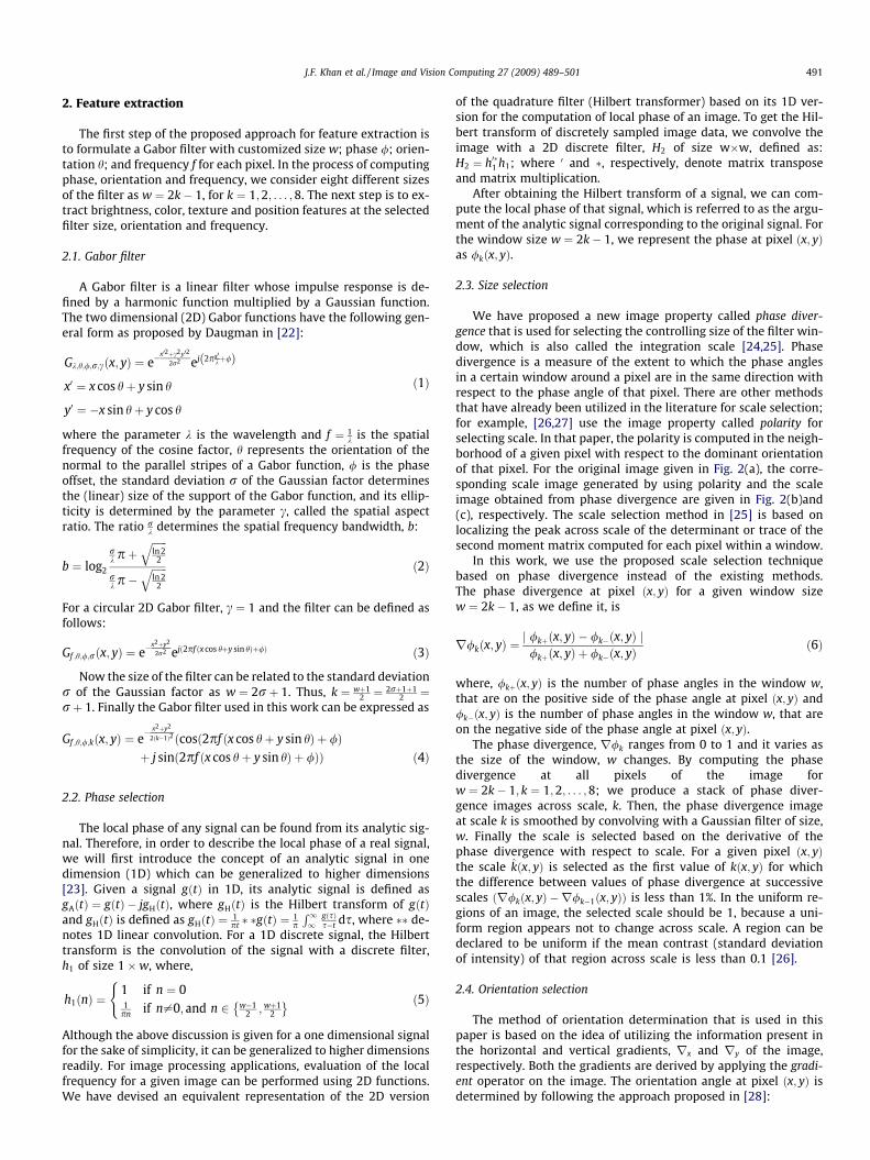
We have proposed a new image property called phase diver-gence that is used for selecting the controlling size of the filter win-dow, which is also called the integration scale [24,25]. Phasedivergence is a measure of the extent to which the phase anglesin a certain window around a pixel are in the same direction withrespect to the phase angle of that pixel. There are other methodsthat have already been utilized in the literature for scale selection;for example, [26,27] use the image property called polarity forselecting scale. In that paper, the polarity is computed in the neigh-borhood of a given pixel with respect to the dominant orientationof that pixel. For the original image given in Fig. 2(a), the corre-sponding scale image generated by using polarity and the scaleimage obtained from phase divergence are given in Fig. 2(b)and(c), respectively. The scale selection method in [25] is based onlocalizing the peak across scale of the determinant or trace of thesecond moment matrix computed for each pixel within a window.

In this work, we use the proposed scale selection techniquebased on phase divergence instead of the existing methods.The phase divergence at pixel ðx; yÞ for a given window sizew ¼ 2k� 1, as we define it, is

r/kðx; yÞ ¼j /kþðx; yÞ � /k�ðx; yÞ j/kþðx; yÞ þ /k�ðx; yÞ

ð6Þ

where, /kþðx; yÞ is the number of phase angles in the window w,that are on the positive side of the phase angle at pixel ðx; yÞ and/k�ðx; yÞ is the number of phase angles in the window w, that areon the negative side of the phase angle at pixel ðx; yÞ.

The phase divergence, r/k ranges from 0 to 1 and it varies asthe size of the window, w changes. By computing the phasedivergence at all pixels of the image forw ¼ 2k� 1; k ¼ 1;2; . . . ;8; we produce a stack of phase diver-gence images across scale, k. Then, the phase divergence imageat scale k is smoothed by convolving with a Gaussian filter of size,w. Finally the scale is selected based on the derivative of thephase divergence with respect to scale. For a given pixel ðx; yÞthe scale kðx; yÞ is selected as the first value of kðx; yÞ for whichthe difference between values of phase divergence at successivescales ðr/kðx; yÞ � r/k�1ðx; yÞÞ is less than 1%. In the uniform re-gions of an image, the selected scale should be 1, because a uni-form region appears not to change across scale. A region can bedeclared to be uniform if the mean contrast (standard deviationof intensity) of that region across scale is less than 0.1 [26].

2.4. Orientation selection

The method of orientation determination that is used in thispaper is based on the idea of utilizing the information present inthe horizontal and vertical gradients, rx and ry of the image,respectively. Both the gradients are derived by applying the gradi-ent operator on the image. The orientation angle at pixel ðx; yÞ isdetermined by following the approach proposed in [28]:

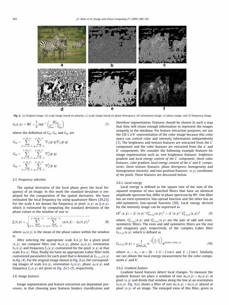
Fig. 2. (a) Original image, (b) scale image based on polarity, (c) scale image based on phase divergence, (d) orientation image, (e) phase image, and (f) frequency image.


hkðx; yÞ ¼ 90�þ 1

2tan�1 2Gxy

Gxx � Gyy

� �ð7Þ

where the definition of Gxy;Gxx and Gyy are

Gxy ¼Xxþðk�1Þ

p¼x�ðk�1Þ

Xyþðk�1Þ

q¼y�ðk�1Þrxðp; qÞryðp; qÞ

Gxx ¼Xxþðk�1Þ

p¼x�ðk�1Þ

Xyþðk�1Þ

q¼y�ðk�1Þr2

x ðp; qÞ

Gyy ¼Xxþðk�1Þ

p¼x�ðk�1Þ

Xyþðk�1Þ

q¼y�ðk�1Þr2

yðp; qÞ

2.5. Frequency selection

The spatial derivative of the local phase gives the local fre-quency of an image. In this work the standard deviation is em-ployed for the computation of the spatial derivative. We haveestimated the local frequency by using quadrature filters [29,23].For the scale k we denote the frequency at pixel ðx; yÞ as fkðx; yÞ,which is estimated by computing the standard deviation of thephase values in the window of size w:

fkðx; yÞ ¼

ffiffiffiffiffiffiffiffiffiffiffiffiffiffiffiffiffiffiffiffiffiffiffiffiffiffiffiffiffiffiffiffiffiffiffiffiffiffiffiffiffiffiffiffiffiffiffiffiffiffiffiffiffiffiffiffiffiffiffiffiffiffiffiffiffiffiffiffiffiffiffiffiffiffiffiffiffiffiffiffiffiffiffiffiffiffiffiffiffiffiXxþfkðx;yÞ�1g

p¼x�fkðx;yÞ�1g

Xyþfkðx;yÞ�1g

q¼y�fkðx;yÞ�1gð/ðx; yÞ � �/kðx; yÞÞ2

vuut ð8Þ

where �/kðx; yÞ is the mean of the phase values within the windoww.

After selecting the appropriate scale kðx; yÞ for a given pixelðx; yÞ, we compute filter size wkðx; yÞ, phase /kðx; yÞ, orientationhkðx; yÞ and frequency f kðx; yÞ customized for the pixel ðx; yÞ at thatscale kðx; yÞ. Thus, finally we have an appropriate Gabor filter withcustomized parameters for each pixel that is denoted as Gf ;h;/;kðx; yÞin Eq. (4). For the original image shown in Fig. 2(a), the correspond-ing images of scale kðx; yÞ, orientation hkðx; yÞ, phase /kðx; yÞ andfrequency f kðx; yÞ are given in Fig. 2(c)–(f), respectively.

2.6. Image features

Image segmentation and feature extraction are dependant pro-cesses, in that choosing poor features hinders classification and

therefore segmentation. Features should be chosen in such a waythat they will retain enough information to represent the imagesuniquely in the database. For feature extraction purposes, we usethe CIE L*a*b* representation of the color image because this colorspace can control color and intensity information independently[1]. The brightness and texture features are extracted from the L*

component and the color features are extracted from the a* andb* components. We consider the following example features forimage segmentation such as, two brightness features: brightnessgradient and local energy content of the L* component; three colorfeatures: color gradient, local energy content of the a* and b* compo-nents; three texture features: phase divergence, homogeneity andhomogeneous intensity; and two position features: ðx; yÞ coordinatesof the pixels. These features are discussed below.

2.6.1. Local energyLocal energy is defined as the square root of the sum of the

squared response of two matched filters that have an identicalamplitude spectrum but, differ in phase spectrum by 90�. One filterhas an even-symmetric line-spread function and the other has anodd-symmetric line-spread function [30]. Local energy derivedfor the intensity image can be expressed as

LEL� ðx; yÞ ¼ ðL�ðx; yÞ��Gok;h;/;f ðx; yÞÞ

2 þ ðL�ðx; yÞ��Gek;h;/;f ðx; yÞÞ

2 ð9Þ

where, Gok;h;/;f ðx; yÞ and Ge

k;h;/;f ðx; yÞ are the pair of odd and even-symmetric filters. The even and odd symmetric filters are the realand imaginary part, respectively, of the complex Gabor filterGk;h;/;f ðx; yÞ, which is defined as

Gk;h;/;f ðx; yÞ ¼1

2prxrye�1

2x2

r2xþy2

r2y

� �ejð2pUxþ2pVyþ/Þ ð10Þ

where rx ¼ ry ¼ w ¼ 2k� 1;U ¼ f cos h and V ¼ f sin h. Similarlywe can obtain the local energy measurement for the color compo-nents a* and b*.

2.6.2. Gradient featureGradient based features detect local changes. To measure the

gradient feature we place a window of size wkðx; yÞ � wkðx; yÞ atpixel ðx; yÞ and divide that window along the line at an orientationhkðx; yÞ. Fig. 3(a) shows a filter of size wkðx; yÞ � wkðx; yÞ placed atpixel ðx; yÞ of an image. The enlarged view of this filter, given in

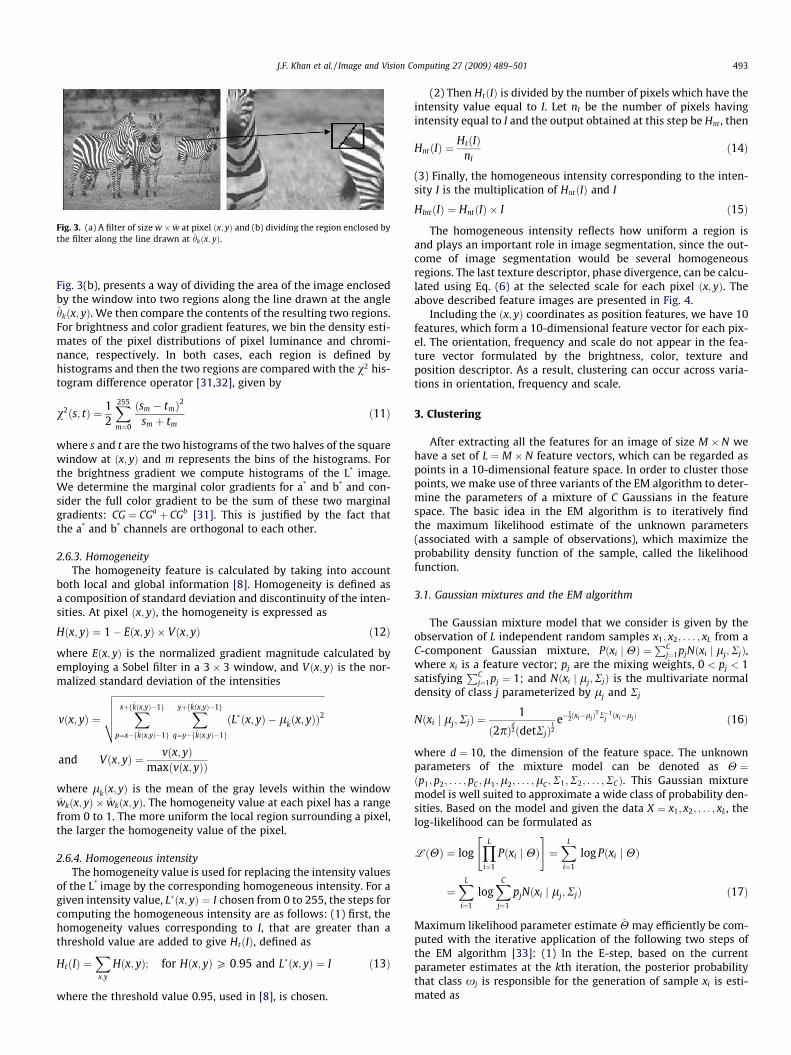
Fig. 3. (a) A filter of size w� w at pixel ðx; yÞ and (b) dividing the region enclosed bythe filter along the line drawn at hkðx; yÞ.


Fig. 3(b), presents a way of dividing the area of the image enclosedby the window into two regions along the line drawn at the anglehkðx; yÞ. We then compare the contents of the resulting two regions.For brightness and color gradient features, we bin the density esti-mates of the pixel distributions of pixel luminance and chromi-nance, respectively. In both cases, each region is defined byhistograms and then the two regions are compared with the v2 his-togram difference operator [31,32], given by

v2ðs; tÞ ¼ 12

X255

m¼0

ðsm � tmÞ2

sm þ tmð11Þ

where s and t are the two histograms of the two halves of the squarewindow at ðx; yÞ and m represents the bins of the histograms. Forthe brightness gradient we compute histograms of the L* image.We determine the marginal color gradients for a* and b* and con-sider the full color gradient to be the sum of these two marginalgradients: CG ¼ CGa þ CGb [31]. This is justified by the fact thatthe a* and b* channels are orthogonal to each other.

2.6.3. HomogeneityThe homogeneity feature is calculated by taking into account

both local and global information [8]. Homogeneity is defined asa composition of standard deviation and discontinuity of the inten-sities. At pixel ðx; yÞ, the homogeneity is expressed as

Hðx; yÞ ¼ 1� Eðx; yÞ � Vðx; yÞ ð12Þ

where Eðx; yÞ is the normalized gradient magnitude calculated byemploying a Sobel filter in a 3 � 3 window, and Vðx; yÞ is the nor-malized standard deviation of the intensities

vðx; yÞ ¼

ffiffiffiffiffiffiffiffiffiffiffiffiffiffiffiffiffiffiffiffiffiffiffiffiffiffiffiffiffiffiffiffiffiffiffiffiffiffiffiffiffiffiffiffiffiffiffiffiffiffiffiffiffiffiffiffiffiffiffiffiffiffiffiffiffiffiffiffiffiffiffiffiffiffiffiffiffiffiffiffiffiffiffiffiffiffiffiffiffiffiffiXxþfkðx;yÞ�1g

p¼x�fkðx;yÞ�1g

Xyþfkðx;yÞ�1g

q¼y�fkðx;yÞ�1g

ðL�ðx; yÞ � lkðx; yÞÞ2

vuuutand Vðx; yÞ ¼ vðx; yÞ

maxðvðx; yÞÞ

where lkðx; yÞ is the mean of the gray levels within the windowwkðx; yÞ � wkðx; yÞ. The homogeneity value at each pixel has a rangefrom 0 to 1. The more uniform the local region surrounding a pixel,the larger the homogeneity value of the pixel.

2.6.4. Homogeneous intensityThe homogeneity value is used for replacing the intensity values

of the L* image by the corresponding homogeneous intensity. For agiven intensity value, L�ðx; yÞ ¼ I chosen from 0 to 255, the steps forcomputing the homogeneous intensity are as follows: (1) first, thehomogeneity values corresponding to I, that are greater than athreshold value are added to give HtðIÞ, defined as

HtðIÞ ¼Xx;y

Hðx; yÞ; for Hðx; yÞP 0:95 and L�ðx; yÞ ¼ I ð13Þ

where the threshold value 0.95, used in [8], is chosen.

(2) Then HtðIÞ is divided by the number of pixels which have theintensity value equal to I. Let nI be the number of pixels havingintensity equal to I and the output obtained at this step be Hnt , then

HntðIÞ ¼HtðIÞ

nIð14Þ

(3) Finally, the homogeneous intensity corresponding to the inten-sity I is the multiplication of HntðIÞ and I

HIntðIÞ ¼ HntðIÞ � I ð15Þ

The homogeneous intensity reflects how uniform a region isand plays an important role in image segmentation, since the out-come of image segmentation would be several homogeneousregions. The last texture descriptor, phase divergence, can be calcu-lated using Eq. (6) at the selected scale for each pixel ðx; yÞ. Theabove described feature images are presented in Fig. 4.

Including the ðx; yÞ coordinates as position features, we have 10features, which form a 10-dimensional feature vector for each pix-el. The orientation, frequency and scale do not appear in the fea-ture vector formulated by the brightness, color, texture andposition descriptor. As a result, clustering can occur across varia-tions in orientation, frequency and scale.

3. Clustering

After extracting all the features for an image of size M � N wehave a set of L ¼ M � N feature vectors, which can be regarded aspoints in a 10-dimensional feature space. In order to cluster thosepoints, we make use of three variants of the EM algorithm to deter-mine the parameters of a mixture of C Gaussians in the featurespace. The basic idea in the EM algorithm is to iteratively findthe maximum likelihood estimate of the unknown parameters(associated with a sample of observations), which maximize theprobability density function of the sample, called the likelihoodfunction.

3.1. Gaussian mixtures and the EM algorithm

The Gaussian mixture model that we consider is given by theobservation of L independent random samples x1; x2; . . . ; xL from aC-component Gaussian mixture, Pðxi j HÞ ¼

PCj¼1pjNðxi j lj;RjÞ,

where xi is a feature vector; pj are the mixing weights, 0 < pj < 1satisfying

PCj¼1pj ¼ 1; and Nðxi j lj;RjÞ is the multivariate normal

density of class j parameterized by lj and Rj

Nðxi j lj;RjÞ ¼1

ð2pÞd2ðdetRjÞ

12

e�12ðxi�ljÞ

TR�1j ðxi�ljÞ ð16Þ

where d ¼ 10, the dimension of the feature space. The unknownparameters of the mixture model can be denoted as H ¼ðp1;p2; . . . ;pC ;l1;l2; . . . ;lC ;R1;R2; . . . ;RCÞ. This Gaussian mixturemodel is well suited to approximate a wide class of probability den-sities. Based on the model and given the data X ¼ x1; x2; . . . ; xL, thelog-likelihood can be formulated as

LðHÞ ¼ logYL

i¼1

Pðxi j HÞ" #

¼XL

i¼1

log Pðxi j HÞ

¼XL

i¼1

logXC

j¼1

pjNðxi j lj;RjÞ ð17Þ

Maximum likelihood parameter estimate H may efficiently be com-puted with the iterative application of the following two steps ofthe EM algorithm [33]: (1) In the E-step, based on the currentparameter estimates at the kth iteration, the posterior probabilitythat class xj is responsible for the generation of sample xi is esti-mated as

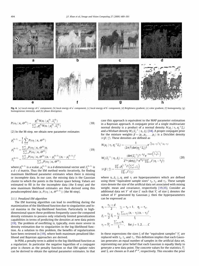
Fig. 4. (a) Local energy of L* component, (b) local energy of a* component, (c) local energy of b* component, (d) Brightness gradient, (e) color gradient, (f) homogeneity, (g)homogeneous intensity, and (h) phase divergence.


Pðxj j xi;HðkÞÞ ¼

pðkÞj Nðxi j lðkÞj ;RðkÞj ÞPCj¼1pðkÞj Nðxi j lðkÞj ;RðkÞj Þ

ð18Þ

(2) In the M-step, we obtain new parameter estimates

pðkþ1Þj ¼ 1

L

XL

i¼1

Pðxj j xi;HðkÞÞ

lðkþ1Þj ¼

PLi¼1Pðxj j xi;H

ðkÞÞxiPLi¼1Pðxj j xi;H

ðkÞÞ

Rðkþ1Þj ¼

PLi¼1Pðxj j xi;H

ðkÞÞðxi � lðkþ1Þj Þðxi � lðkþ1Þ

j ÞTPLi¼1Pðxj j xi;H

ðkÞÞ

ð19Þ

where pðkþ1Þj is a scalar, lðkþ1Þ

j is a d-dimensional vector and Rðkþ1Þj is

a d� d matrix. Thus the EM method works iteratively, for findingmaximum likelihood parameter estimates when there is missingor incomplete data. In our case, the missing data is the Gaussiancluster to which the points in the feature space belong. Values areestimated to fill in for the incomplete data (the E-step) and thenew maximum likelihood estimates are then derived using thispseudocompleted data ðxi; Pðxj j xi;H

ðkþ1ÞÞÞ (the M-step).

3.1.1. Penalized EM algorithmThe EM learning algorithm can lead to overfitting during the

maximization of the likelihood function due to singularities and lo-cal maxima in the log-likelihood function. Particularly in high-dimensional spaces these problems frequently cause the computeddensity estimates to possess only relatively limited generalizationcapabilities in terms of predicting the densities at new data points[19]. The problem of overfitting is, typically, even more severe indensity estimation due to singularities in the log-likelihood func-tion. As a solution to this problem, the benefits of regularizationhave been reviewed in [19], where both maximum penalized like-lihood and Bayesian approaches are derived.

In PEM, a penalty term is added to the log-likelihood function asa regularizer. In particular the negative logarithm of a conjugateprior is chosen as the penalty function so that EM update rulescan be derived to obtain the optimal parameter estimates. In that

case this approach is equivalent to the MAP parameter estimationin a Bayesian approach. A conjugate prior of a single multivariatenormal density is a product of a normal density Nðlj j mj;g�1

j RjÞand a Wishart density WjðR�1

j j aj; bjÞ [34]. A proper conjugate priorfor the mixture weights ~p ¼ ðp1; p2; . . . ; pCÞ is a Dirichlet densityDð~p j~cÞ. These densities are defined as

Nðlj j mj;g�1j RjÞ ¼

1

ð2pÞd2ðdet½g�1

j Rj�Þ12

e�gj2 ðlj�mjÞT R�1

j ðlj�mjÞ

WjðR�1j j aj;bjÞ ¼

ðdet½R�1j �Þ

aj�dþ12 e�trace

b�1j

R�1j

2

� �2ajdðdetbjÞ

ajpdðd�1Þ

4Qd

k¼1Cðaj � k�12 Þ

Dð~p j~cÞ ¼QC

j¼1pcj�1j C

PCj¼1cj

� �QC

j¼1CðcjÞ

ð20Þ

where aj; bj; cj;gj and mj are hyperparameters which are definedusing three ‘‘equivalent sample sizes” sp; sl and sR. These samplesizes denote the size of the artificial data set associated with mixingweight, mean and covariance, respectively [19,35]. Consider anadditional data set Y� of size L0 such that Y�j of size lj denotes thesubset of Y� generated by Gaussian j, then the hyperparameterscan be expressed as

aj ¼sR þ d

2; cj ¼ sp þ 1; gj ¼ sl;

bj ¼sR

2eSj ¼

sR

2

Pxi2Y�jðxi � mjÞðxi � mjÞT

lj;

mj ¼ Y�j ¼P

xi2Y�jxi

lj; for j ¼ 1;2; . . . ; C

In these expressions the sizes lj of the ‘‘equivalent samples” Y�j arereplaced with sp; sl and sR. This definition implies that each Gauss-ian generates an equal number of samples in the artificial data set,representing our prior belief that each Gaussian is equally likely togenerate a new data point. The concrete values for the statistics, Y�jand eSj are chosen as 0 and Id�d, respectively. This encodes the prior


belief that centers are zero and the covariance matrix is the unitmatrix. Next the degree of regularization is determined by varyingthe equivalent sample sizes and those values are set to sp ¼ sl ¼ 0and sR ¼ 0:1 as suggested in [19].

For the PEM algorithm, the prior of the Gaussian mixture is

pj ¼ Dð~p j~cÞYC

j¼1

Nðlj j mj;g�1j RjÞWjðR�1

j j aj;bjÞ ð21Þ

In the case of PEM [19], (1) the MAP parameter estimate maximizesthe following log-posterior function

LpðHÞ ¼XL

i¼1

logXC

j¼1

pjNðxi j lj;RjÞ þ logDð~p j~cÞ

þXC

j¼1

½log Nðlj j mj;g�1j RjÞ þ log WjðR�1

j j aj;bjÞ� ð22Þ

(2) the E-step remains identical to the EM algorithm and (3) theM-step becomes

pðkþ1Þj ¼

PLi¼1Pðxj j xi;H

ðkÞÞ þ cj � 1

LþPC

j¼1cj � C

lðkþ1Þj ¼

PLi¼1Pðxj j xi;H

ðkÞÞxi þ gjmjPLi¼1Pðxj j xi;H

ðkÞÞ þ gj

Rðkþ1Þj ¼

PLi¼1Pðxj j xi;H


j ÞT þ gjðlðkþ1Þj � mjÞðlðkþ1Þ

j � mjÞT þ 2bjPLi¼1Pðxj j xi;H

ðkÞÞ þ 2aj � d

ð23Þ

Though it is apparent from the above update in the M-step, only afew additional computations are required for optimizing the maxi-mum penalized likelihood in comparison to standard EM, in ouranalysis we find that the described PEM procedure leads to fasterconvergence. Moreover, Rj does not approach the null matrix, as of-ten happens in case of standard EM.

3.1.2. Penalized stochastic EM algorithmTo avoid some defects of maximum likelihood estimation

using EM, a random version called stochastic EM (SEM) has beenintroduced in [36], where instead of estimating missing dataPðxj j xi;H

ðkþ1ÞÞ, it is simulated from their conditional distribu-tion, i.e. the multinomial distribution with mixing weights. Thismethod is well known as Gibbs sampling or Bayesian sampling. Inthis approach, the unknown parameters Hðkþ1Þ at any iterationare considered to be random variables which are sampled inthe M-step, and the E-step is performed using these samples.During sampling either one sample or several samples can bedrawn. The method is known as stochastic EM (SEM) when onlyone sample is drawn, and Monte Carlo EM (MCEM) when severalsamples are drawn. In the penalized SEM, the new parametervalues are generated according to

~pðkþ1Þ � DðcqÞ; R�1ðkþ1Þ

j �Wjðaqj ;b

qj Þ

lðkþ1Þj � Nðmq

j ;gq�1

j R0jÞ; for j ¼ 1;2; . . . ; Cð24Þ

where q defines a unique partitioning of the data set X into C Gaus-sians: q ¼ ðq1;q2; . . . ;qCÞ with j qj j as the size of qj, subset of X,that is generated by Gaussian j. The definition of aq

j ;bqj ;g

qj and cq

j

are as follows:

aqj ¼ajþ

jqj j2; bq

j ¼ bjþ12jqj j eSj þ

12

gj jqj jgjþ jqj j

ðmj�XjÞðmj�XjÞT;

gqj ¼gjþ jqj j;

mqj ¼

1gjþ jqj j

ðgjmjþ jqj jXjÞ; cq¼ðc1þ jq1 j;c2þ jq2 j; . . . ;cCþ jqC jÞ

where Xj ¼P

xi2qjxi

jqj jand eSj ¼

Pxi2qj

ðxi�XjÞðxi�XjÞT

jqj j. The values of the

hyperparameters are chosen in the same way as in PEM.

3.1.3. Inverse EM algorithmIn the IEM algorithm [20], the basic modification consists of vir-

tually updating the observed covariance matrices in the first stageand then, in the second stage, the reversed updating of the esti-mated covariances. This algorithm is devoted to the estimation ofthe parameters of multivariate Gaussian mixture where the covari-ance matrices are constrained to have a linear structure such asToeplitz, Hankel, or circular constraints. The E-step for IEM is thesame as EM and the M-step updates are as follows. (1) At first, abasis fQgM

l¼1 (independent matrices, not necessarily orthogonal) of

the constrained linear space S is provided, where M is the dimen-sion of the constrained linear space. (2) The parameters are up-dated at the ðkþ 1Þth iteration as

pðkþ1Þj ¼ 1

L

XL

i¼1Pðxj j xi;H

ðkÞÞ

lðkþ1Þj ¼

PLi¼1Pðxj j xi;H

ðkÞÞxiPLi¼1Pðxj j xi;H

ðkÞÞ

Aðkþ1Þj ¼

PLi¼1Pðxj j xi;H


j ÞTPLi¼1Pðxj j xi;H

ðkÞÞ

Cðkþ1Þj ¼

Aðkþ1Þj þ tj

jqj jE�1

j

1þ tjþdþ1jqj j

ð25Þ

where Aj is the observed weighted covariance matrix, Cj is theempirical covariance matrix, Ej is a positive definite matrix belongto the class j, and tj is the degree of the freedom of the distributionfor Cj, which is the inverse Wishart density, IW

Cj � IWdðtj; EjÞ / ðdet½C�1j �Þ

tjþdþ12 e�trace

tjC�1j

E�1j

2

� �: ð26Þ

(3) Finally, the unknown covariance matrices are updated as

Rðkþ1Þj ¼ RðkÞj þ akDj ð27Þ

where Dj ¼P

xlQ l � RðkÞj is the amount of increment needed in RðkÞj

and ak is the step size. Now, the vector x needs to be computedwhich can be expressed as x ¼ B�1b. Having the basis fQgM

l¼1 of spaceS, there are the following linear systems to be solved for each classto find the vector x:


XM

l¼1

xlðtrace½RðkÞ�1

j Q lRðkÞ�1

j Q i�Þ ¼ trace½RðkÞ�1

j CðkÞj RðkÞ�1

j Q i�;

for i ¼ 1; . . . ;M

This system can be put in an algebraic form: Bx ¼ b, where the ma-trix B and the vector b are calculated according to the following:

Bil ¼ trace½RðkÞ�1

j Q lRðkÞ�1

j Q i�

bi ¼ trace½RðkÞ�1

j CðkÞj RðkÞ�1

j Q i�ð28Þ

The step size ak is calculated as

ak ¼trace½RðkÞ

�1

j DjRðkÞ�1

j Dj�

2trace½RðkÞ�1

j DjRðkÞ�1

j DjRðkÞ�1

j CðkÞj � � trace½RðkÞ�1

j DjRðkÞ�1

j Dj�ð29Þ

(4) If the updated Rðkþ1Þj is non-positive, then ak is changed by ak

2 andthe algorithm returns to step 3, otherwise the iteration number k isincremented by one and the algorithm iterates back from step 2.

3.1.4. Penalized inverse EM algorithmIn this paper, we have incorporated the favorable features of

both the PEM and the IEM to formulate PIEM. Similar to the IEMalgorithm, the PIEM algorithm also starts with the generation ofa basis fQgM

l¼1 of the constrained linear space S. Then at the sec-ond step the parameters are updated following the PEM algo-rithm [19]:

pðkþ1Þj ¼

PLi¼1Pðxj j xi;H

ðkÞÞ þ cj � 1

LþPC

j¼1cj � C

lðkþ1Þj ¼

PLi¼1Pðxj j xi;H

ðkÞÞxi þ gjmjPLi¼1Pðxj j xi;H

ðkÞÞ þ gj

Cðkþ1Þj ¼

PLi¼1Pðxj j xi;H


j ÞT þ gjðlðkþ1Þj � mjÞðlðkþ1Þ

j � mjÞT þ 2bjPLi¼1Pðxj j xi;H

ðkÞÞ þ 2aj � d

ð30Þ

Finally the covariance matrices of the Gaussian mixture models atthe ðkþ 1Þth iteration are calculated by following steps 3 and 4 ofthe inverse EM algorithm. This algorithm is found to converge muchfaster than the EM algorithms discussed previously. Moreover, theclustering performance is proved to be the best for the proposedPIEM algorithm.

3.2. Clustering using PEM, PSEM and PIEM

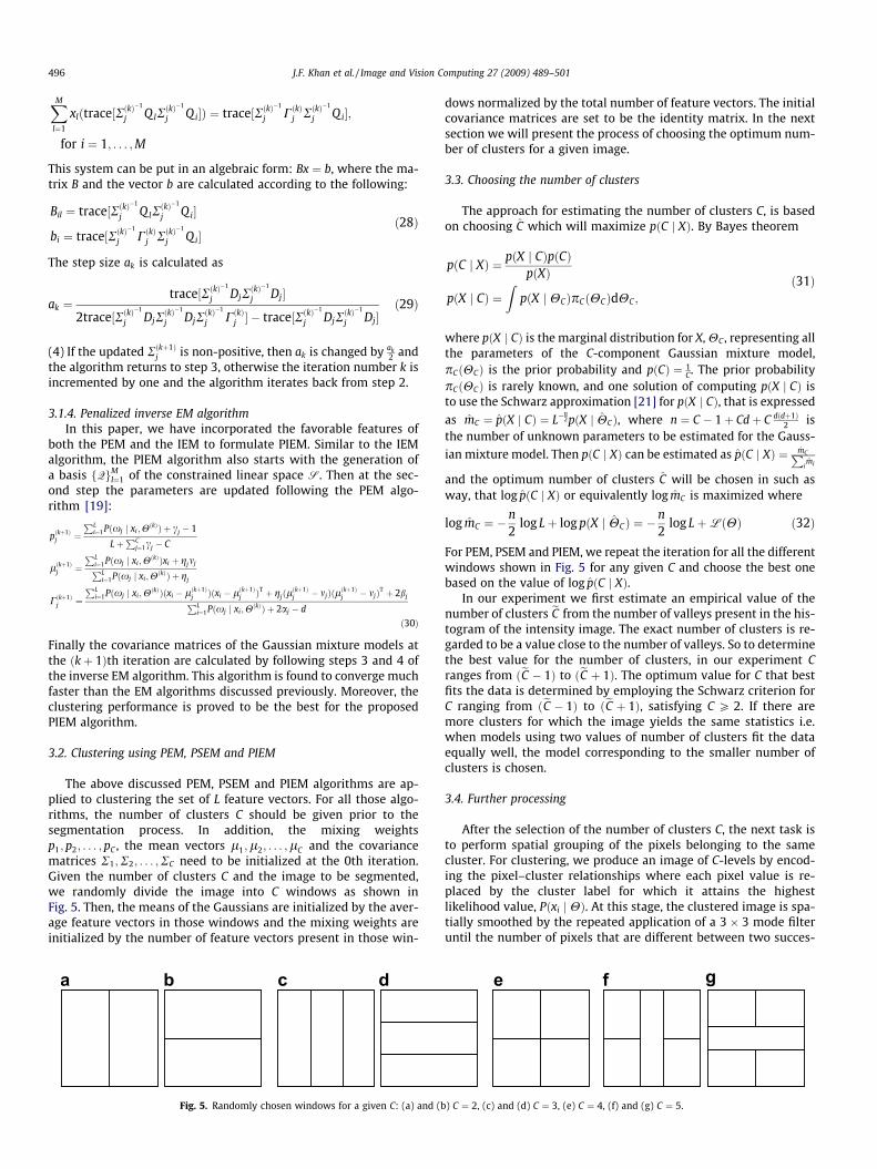
The above discussed PEM, PSEM and PIEM algorithms are ap-plied to clustering the set of L feature vectors. For all those algo-rithms, the number of clusters C should be given prior to thesegmentation process. In addition, the mixing weightsp1; p2; . . . ; pC , the mean vectors l1;l2; . . . ;lC and the covariancematrices R1;R2; . . . ;RC need to be initialized at the 0th iteration.Given the number of clusters C and the image to be segmented,we randomly divide the image into C windows as shown inFig. 5. Then, the means of the Gaussians are initialized by the aver-age feature vectors in those windows and the mixing weights areinitialized by the number of feature vectors present in those win-

Fig. 5. Randomly chosen windows for a given C: (a) and (b

dows normalized by the total number of feature vectors. The initialcovariance matrices are set to be the identity matrix. In the nextsection we will present the process of choosing the optimum num-ber of clusters for a given image.

3.3. Choosing the number of clusters

The approach for estimating the number of clusters C, is basedon choosing C which will maximize pðC j XÞ. By Bayes theorem

pðC j XÞ ¼ pðX j CÞpðCÞpðXÞ

pðX j CÞ ¼Z

pðX j HCÞpCðHCÞdHC ;

ð31Þ

where pðX j CÞ is the marginal distribution for X, HC , representing allthe parameters of the C-component Gaussian mixture model,pCðHCÞ is the prior probability and pðCÞ ¼ 1

C. The prior probabilitypCðHCÞ is rarely known, and one solution of computing pðX j CÞ isto use the Schwarz approximation [21] for pðX j CÞ, that is expressed

as mC ¼ pðX j CÞ ¼ L�n2pðX j HCÞ, where n ¼ C � 1þ Cdþ C dðdþ1Þ

2 isthe number of unknown parameters to be estimated for the Gauss-ian mixture model. Then pðC j XÞ can be estimated as pðC j XÞ ¼ mCP

imi

and the optimum number of clusters C will be chosen in such asway, that log pðC j XÞ or equivalently log mC is maximized where

log mC ¼ �n2

log Lþ log pðX j HCÞ ¼ �n2

log LþLðHÞ ð32Þ

For PEM, PSEM and PIEM, we repeat the iteration for all the differentwindows shown in Fig. 5 for any given C and choose the best onebased on the value of log pðC j XÞ.

In our experiment we first estimate an empirical value of thenumber of clusters eC from the number of valleys present in the his-togram of the intensity image. The exact number of clusters is re-garded to be a value close to the number of valleys. So to determinethe best value for the number of clusters, in our experiment Cranges from ðeC � 1Þ to ðeC þ 1Þ. The optimum value for C that bestfits the data is determined by employing the Schwarz criterion forC ranging from ðeC � 1Þ to ðeC þ 1Þ, satisfying C P 2. If there aremore clusters for which the image yields the same statistics i.e.when models using two values of number of clusters fit the dataequally well, the model corresponding to the smaller number ofclusters is chosen.

3.4. Further processing

After the selection of the number of clusters C, the next task isto perform spatial grouping of the pixels belonging to the samecluster. For clustering, we produce an image of C-levels by encod-ing the pixel–cluster relationships where each pixel value is re-placed by the cluster label for which it attains the highestlikelihood value, Pðxi j HÞ. At this stage, the clustered image is spa-tially smoothed by the repeated application of a 3 � 3 mode filteruntil the number of pixels that are different between two succes-

) C ¼ 2, (c) and (d) C ¼ 3, (e) C ¼ 4, (f) and (g) C ¼ 5.


sive images is less than 1%. The mode filter yields an output equalto the value that occurs most often in the 3 � 3 window. In thesmoothed image, there may be some regions of a few pixels locatedinside another large region. Those smaller regions are required tobe classified as the member of that large region to produce homo-geneous and united regions in the segmented image, which isaccomplished by employing a connected-component algorithm[37].

4. Experimental results

We have applied the proposed scheme for the segmentation ofseveral images. In this section, we present the experimental resultsobtained at different stages of the clustering algorithm. We havetested all four clustering algorithms presented in this papernamely PEM, PSEM, IEM and PIEM. Among those four algorithmsIEM fails to converge for the experimental data used for this workand thus the segmentation results yielded from IEM does not ap-pear to be meaningful and hence usable. Therefore, we did notpresent and discuss the results of segmentation obtained fromIEM algorithm.

For the segmentation utilizing PEM, PSEM and PIEM, at first thehistogram of the intensity image of an color image is analyzed topredict the approximate number of clusters present in the image.From the histogram of the image shown in Fig. 2(a), the estimated

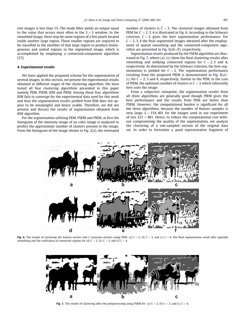
Fig. 6. The results of clustering the feature vectors into C Gaussian clusters using PEMsmoothing and the unification of connected regions for (d) C ¼ 2, (e) C ¼ 3, and (f) C ¼

Fig. 7. The results of clustering after the postprocessing

number of clusters is eC ¼ 3. The clustered images obtained fromPEM for C ¼ 2;3;4 is illustrated in Fig. 6. According to the Schwarzcriterion, C ¼ 2 gives the best segmentation performance. ForC ¼ 2;3;4 the final segmented images obtained after the employ-ment of spatial smoothing and the connected-component algo-rithm are presented in Fig. 6(d)–(f), respectively.

Segmentation results produced by the PSEM algorithm are illus-trated in Fig. 7, where (a)–(c) show the final clustering results aftersmoothing and unifying connected regions for C ¼ 2;3 and 4,respectively. As determined by the Schwarz criterion, the best seg-mentation is yielded for C ¼ 3. The segmentation performanceresulting from the proposed PIEM is demonstrated in Fig. 8(a)–(c) for C ¼ 2;3 and 4, respectively. Similar to the PEM, in the caseof PIEM, the optimum number of clusters is C ¼ 2 which inherentlybest suits the image.

From a subjective viewpoint, the segmentation results fromall three algorithms are generally good though PIEM gives thebest performance and the results from PEM are better thanPSEM. However, the computational burden is significant for allthe three algorithms, because the number of feature samples isvery large, L ¼ 154;401 for the images used in our experimentof size 321 � 481. Hence, to reduce the computational cost with-out compromising the quality of the segmentation, we analyzethe clustering of a sub-sampled version of the original dataset. In order to formulate a good representative fragment of

: (a) C ¼ 2, (b) C ¼ 3, and (c) C ¼ 4. The final segmentation result after spatially4.

using PSEM for: (a) C ¼ 2, (b) C ¼ 3, and (c) C ¼ 4.

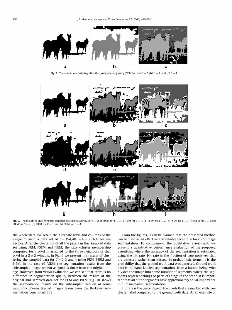
Fig. 9. The results of clustering the sampled data using (a) PEM for C ¼ 2, (b) PEM for C ¼ 3, (c) PEM for C ¼ 4, (d) PSEM for C ¼ 2, (e) PSEM for C ¼ 3, (f) PSEM for C ¼ 4, (g)PIEM for C ¼ 2, (h) PIEM for C ¼ 3, and (i) PIEM for C ¼ 4.

Fig. 8. The results of clustering after the postprocessing using PIEM for: (a) C ¼ 2, (b) C ¼ 3, and (c) C ¼ 4.


the whole data, we retain the alternate rows and columns of theimage to yield a data set of L ¼ 154;401� 4 ¼ 38;600 featurevectors. After the clustering of all the pixels in this sampled dataset using PEM, PSEM and PIEM; the pixel–cluster membershipcomputed for a pixel is assigned to the three neighbors of thatpixel in a 2 � 2 window. In Fig. 9 we present the results of clus-tering the sampled data for C ¼ 2;3 and 4 using PEM, PSEM andPIEM. In the case of PSEM, the segmentation results from thesubsampled image are not as good as those from the original im-age. However, from visual evaluation we can see that there is nodifference in segmentation quality between the results of theoriginal and sampled data set for PEM and PIEM. Fig. 10 showsthe segmentation results on the subsampled version of somerandomly chosen typical images taken from the Berkeley seg-mentation benchmark [38].

From the figures, it can be claimed that the presented methodcan be used as an effective and reliable technique for color imagesegmentation. To complement the qualitative assessment, wepresent a quantitative performance evaluation of the proposedalgorithm, where the accuracy of the segmentation is estimatedusing the hit rate. Hit rate is the fraction of true positives thatare detected rather than missed. In probabilistic terms, it is theprobability that the ground truth data was detected. Ground truthdata is the hand-labeled segmentations from a human being, whodivides the image into some number of segments, where the seg-ments represent things or parts of things in the scene. It is impor-tant that all of the segments have approximately equal importancein human-marked segmentation.

Hit rate is the percentage of the pixels that are marked with truecluster label compared to the ground truth data. As an example of

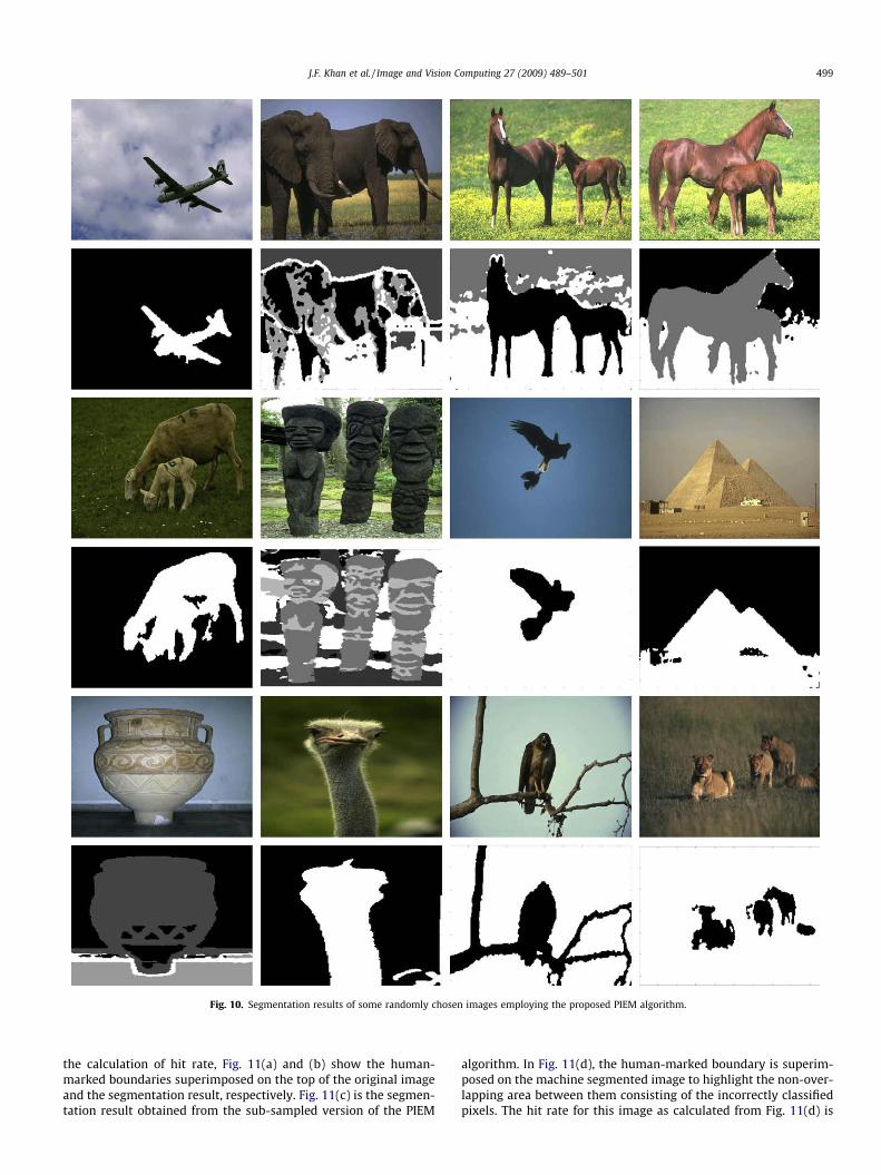
Fig. 10. Segmentation results of some randomly chosen images employing the proposed PIEM algorithm.


the calculation of hit rate, Fig. 11(a) and (b) show the human-marked boundaries superimposed on the top of the original imageand the segmentation result, respectively. Fig. 11(c) is the segmen-tation result obtained from the sub-sampled version of the PIEM

algorithm. In Fig. 11(d), the human-marked boundary is superim-posed on the machine segmented image to highlight the non-over-lapping area between them consisting of the incorrectly classifiedpixels. The hit rate for this image as calculated from Fig. 11(d) is

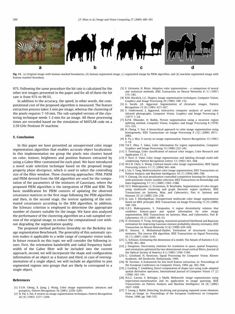
Fig. 11. (a) Original image with human-marked boundaries, (b) human segmented image, (c) segmented image by PIEM algorithm, and (d) machine segmented image withhuman-marked boundary.


97%. Following the same procedure the hit rate is calculated for theother test images presented in the paper and for all of them the hitrate is from 97% to 99.5%.

In addition to the accuracy, the speed, in other words, the com-putational cost of the proposed algorithm is measured. The featureextraction process takes 3 min per image, whereas the clustering ofthe pixels requires 7-10 min. The sub-sampled version of the clus-tering technique needs 1-2 min for an image. All those processingtimes are recorded based on the simulation of MATLAB code on a2.59 GHz Pentium IV machine.

5. Conclusion

In this paper we have presented an unsupervised color imagesegmentation algorithm that enables accurate object localization.In this implementation we group the pixels into clusters basedon color, texture, brightness and position features extracted byusing a Gabor filter customized for each pixel. We have introduceda novel scale selection technique based on the proposed imageproperty phase divergence, which is used to select the controllingsize of the filter window. Three clustering approaches: PEM, PSEMand PIEM derived from the EM algorithm are used for the compu-tation of the parameters of the mixtures of Gaussians, where theproposed PIEM algorithm is the integration of PEM and IEM. Thebasic modification for PIEM consists of updating the observedcovariance matrices in the first stage following the PEM algorithmand then, in the second stage, the reverse updating of the esti-mated covariances according to the IEM algorithm. In addition,the Schwarz criterion is employed to determine the appropriatenumber of clusters suitable for the image. We have also analyzedthe performance of the clustering algorithm on a sub-sampled ver-sion of the original image, to reduce the computational cost with-out degrading the segmentation quality.

The proposed method performs favorably on the Berkeley im-age segmentation Benchmark. The generality of this automatic sys-tem makes it applicable to a wide range of computer vision tasks.In future research on this topic we will consider the following is-sues. First, the orientation bandwidth and radial frequency band-width of the Gabor filter will be included into the currentapproach, second, we will incorporate the shape and configurationinformation of an object as a feature and third, in case of overseg-mentation of a single object, we will include an algorithm to joinsegmented regions into groups that are likely to correspond to asingle object.

References

[1] Y.S.H. Cheng, X. Jiang, J. Wang, Color image segmentation: advances andprospects, Pattern Recognition 34 (2001) 2259–2281.

[2] N. Pal, S. Pal, A review on image segmentation techniques, Pattern Recognition26 (9) (1993) 1277–1294.

[3] E. Littmann, H. Ritter, Adaptive color segmentation – a comparison of neuraland statistical methods, IEEE Transaction on Neural Networks 8 (1) (1997)175–185.

[4] R.M. Haralick, L.G. Shapiro, Image segmentation techniques, Computer Vision,Graphics and Image Processing 29 (1985) 100–132.

[5] A. Sarabi, J.K. Aggarwal, Segmentation of chromatic images, PatternRecognition 13 (6) (1981) 417–427.

[6] S. Underwood, J. Aggarwal, Interactive computer analysis of aerial colorinfrared photographs, Computer Vision, Graphics and Image Processing 6(1977) 1–24.

[7] K.P.R. Ohlander, D. Reddy, Picture segmentation using a recursive regionsplitting method, Computer Vision, Graphics and Image Processing 8 (1978)313–333.

[8] H. Cheng, Y. Sun, A hierarchical approach to color image segmentation usinghomogeneity, IEEE Transactions on Image Processing 9 (12) (2000) 2071–2082.

[9] K. Fu, J. Mui, A survey on image segmentation, Pattern Recognition 13 (1981)3–16.

[10] T.K.Y. Ohta, T. Sakai, Color information for region segmentation, ComputerGraphics and Image Processing 13 (1980) 222–241.

[11] S. Tominaga, Color classification of natural color images, Color Research andApplication 17, 4.

[12] F. Ferri, E. Vidal, Color image segmentation and labeling through multi-editcondensing, Pattern Recognition Letters 13 (1992) 561–568.

[13] W.C.H. Chen, S. Wang, Contrast-based color image segmentation, IEEE SignalProcessing Letters 11 (7) (2004) 641–644.

[14] J. Liu, Y. Yang, Multiresolution color image segmentation, IEEE Transactions onPattern Analysis and Machine Intelligence 16 (7) (1994) 689–700.

[15] Y. Cheung, On rival penalization controlled competitive learning for clusteringwith automatic cluster number selection, IEEE Transactions on Knowledge andData Engineering 17 (11) (2005) 1583–1588.

[16] S.F.S. Makrogiannis, G. Economou, N. Bourbakis, Segmentation of color imagesusing multiscale clustering and graph theoretic region synthesis, IEEETransactions on Systems, Man, and Cybernetics, Part A: Systems andHumans 35 (2) (2005) 224–238.

[17] Q. Luo, T. Khoshgoftaar, Unsupervised multiscale color image segmentationbased on MDL principle, IEEE Transactions on Image Processing 15 (9) (2006)100–104.

[18] G.E.S. Makrogiannis, S. Fotopoulos, A region dissimilarity relation thatcombines feature-space and spatial information for color imagesegmentation, IEEE Transactions on Systems, Man, and Cybernetics, Part B:Cybernetics 35 (1) (2005) 44–53.

[19] D. Ormoneit, V. Tresp, Averaging, maximum penalized likelihood and Bayesianestimation for improving Gaussian mixture probability density estimates, IEEETransaction on Neural Networks 9 (4) (1998) 639–650.

[20] H. Snoussi, A. Mohammad-Djafari, Estimation of structured Gaussianmixtures: The inverse EM algorithm, IEEE Transactions on Signal Processing55 (7) (2007) 3185–3191.

[21] G. Schwarz, Estimating the dimension of a model, The Annals of Statistics 6 (2)(1978) 461–464.

[22] J. Daugman, Uncertainty relations for resolution in space, spatial frequency,and orientation optimized by two-dimensional visual cortical filters, Journal ofthe Optical Society of America A 2 (1985) 1160–1169.

[23] G. Grunland, H. Knutsson, Signal Processing for Computer Vision, KluwerAcademic, AH Dordrecht, Netharlands, 1995.

[24] W. Forstner, A framework for low level feature extraction, in: Proceedings ofthe European Conference on Computer Vision, 1994, pp. 383–394.

[25] J. Garding, T. Lindeberg, Direct computation of shape cues using scale-adaptedspatial derivative operators, International Journal of Computer Vision 17 (2)(1996) 163–191.

[26] H.G.C. Carson, S. Belongie, J. Malik, Blobworld: image segmentation usingexpectation-maximization and its application to image querying, IEEETransactions on Pattern Analysis and Machine Intelligence 24 (8) (2002)1027–1038.

[27] T. Leung, J. Malik, Detecting, localizing and grouping repeated scene elementsfrom an image, in: Proceedings of the European Conference on ComputerVision, 1996, pp. 546–555.


[28] A. Rao, A Taxonomy for Texture Description and Identification, Springer-Verlag, New York, 1990.

[29] T. Leung, J. Malik, Regularized quadrature filters for local frequencyestimation: application to multimodal volume image registration, in:Proceedings of Conference on Vision Modeling and Visualization, 1996, pp.507–514.

[30] M. Morrone, D. Burr, Feature detection in human vision: a phase-dependentenergy model, Proceedings of the Royal Society of London 235 (1280) (1988)221–245.

[31] C.F.D. Martin, J. Malik, Learning to detect natural image boundaries using localbrightness, color, and texture cues, IEEE Transactions on Pattern Analysis andMachine Intelligence 26 (5) (2004) 1–19.

[32] C.T.Y. Rubner, J. Puzicha, J. Buhmann, Empirical evaluation of dissimilaritymeasures for color and texture, International Journal of Computer Vision andImage Understanding 84 (2001) 25–43.

[33] N.L.A. Dempster, D. Rubin, Maximum likelihood from incomplete data via theEM algorithm, Journal of Royal Statistical Society 39 (1) (1977) 1–38.

[34] A. Bruce, H.Y. Gao, Bayesian Theory, Wiley, New York, 1994.[35] D. Heckerman, D. Geiger, Likelihood and parameter priors for

Bayesian networks, Microsoft Research Technical Report MSR-TR-95-54.

[36] G. Celeux, J. Diebolt, The SEM algorithm: a probabilistic teacher algorithmderived from the EM algorithm for the mixture problem, ComputationalStatistics Quarterly 2 (1985) 73–82.

[37] R. Gonzalez, R. Woods, Digital Image Processing, Addison Wesley,Massachusetts, 1993.

[38] D.T.D. Martin, C. Fowlkes, J. Malik, A database of human segmented naturalimages and its application to evaluating segmentation algorithms andmeasuring ecological statistics, in: Proceedings of the Eighth InternationalConference on Computer Vision, 2001, pp. 416–423.

a customized gabor filter for unsupervised color image segmentation

Documents