a correction for total ozone mapping spectrometer profile shape errors at high latitude

JOURNAL OF GEOPHYSICAL RESEARCH, VOL. 102, NO. D7, PAGES 9029-9038, APRIL 20, 1997

A correction for total ozone mapping spectrometer profile shape errors at high latitude

C. G. Wellemeyer, S. L. Taylor, and C. J. Seftor Hughes STX Corporation, Greenbelt, Maryland

R. D. McPeters and P. K. Bhartia

NASA Goddard Space Flight Center, Greenbelt, Maryland

Abstract. The total ozone mapping spectrometer (TOMS) ozone measurement is derived by comparing measured backscatter ultraviolet radiances with theoretical radiances computed using standard climatological ozone profiles. Profile shape errors occur in this algorithm at high optical path lengths whenever the actual vertical ozone distribution differs significantly from the standard profile used. These errors are estimated using radiative transfer calculations and measurements of the actual ozone profile. These estimated errors include a short- term component resulting from day-to-day variability in profile shape that gives rise to a standard deviation of 10% in total column ozone amount, as well as a systematic error in the long-term trend at very high solar zenith angles. The trend error resulting from the long-term changes in the ozone profile shape is estimated using measurements from the solar backscattered ultraviolet instrument. At the maximum retrieval solar zenith angle of 88 ø , these calculations indicate that TOMS long-term ozone depletions may be overestimated by 5% per decade. For trend studies that are restricted to latitudes lower than 60 ø (a maximum of 83 ø solar zenith angle), this error is reduced to no more than 1-2% per decade. Differential impact of the profile shape error at the various TOMS wavelength pai,• 111UlCcttc• LIIdL l../ltOlll[3 1111tJ1111atltJll 111•., g.l,o Ul

high solar zenith angles. An interpolation method internal to TOMS is proposed to extract this information. It improves the retrieval at high solar zenith angle, reducing the short- term variability to a standard deviation of 5%, and essentially eliminates the long-term error. The set of standard profiles used in the algorithm are adjusted based on an analysis of empirical orthogonal functions derived from a composite climatology of Stratospheric Aerosol and Gas Experiment II and balloonsonde profile measurements.

Introduction

The total ozone mapping spectrometer (TOMS) instrument measured total column ozone continuously from its launch onboard the Nimbus 7 spacecraft in late October 1978 until it ceased to function on May 6, 1993. These data were processed as version 6 using an improved long-term instrument calibration in 1991 [Herman et al., 1991a]. A number of long-term ozone trend estimates have been derived using this valuable data set [Stolarski et al., 1991; Herman et al., 1991b]. The latitudinal extent of these trend analyses was limited by the onset of known algorithmic errors in the TOMS retrievals at high solar zenith angles [Klenk et al., 1982]. These error sources include sensitivity to the actual vertical distribution of ozone (profile shape), the temperature dependence of the ozone absorption coefficients, uncertainty in the solar zenith angle itself, and small spherical effects on multiple scattered radiation (spherical geometry is applied only to the primary radiation). Of these possible error sources, the profile shape error is the primary source of uncertainty in the TOMS retrievals at high solar zenith angles.

In the version 6 TOMS retrieval, climatological ozone and temperature profiles for various latitude zones and total ozone

Copyright 1997 by the American Geophysical Union.

Paper number 96JD03965. 0148-0227/97/96JD-03965509.00

amounts are used in a radiative transfer calculation [Dave, 1964] in order to compute radiances with which the measured radiances are compared in the ozone computation [McPeters et al., 1993]. A set of five fixed temperature profiles are used, including one each for low, middle, and high latitudes and a separate temperature profile for each of the 125 and 175 Dob- son unit (DU) ozone profiles which characterize ozone hole conditions. The temperature profiles are used in the radiative transfer calculations to take the temperature dependence of the ozone absorption cross sections into account. Pairs of wavclcngtnb are used in the ozone lculeYd• a•;ux•unn to iTiill- imize errors resulting from aerosols and surface reflectivity effects not taken into account in the radiative transfer calcu-

lation. Differences between the assumed climatological ozone profile and the actual ozone profile lead to errors in total ozone determined using this scheme at high solar zenith angles. Longer wavelength pairs are used at higher solar zenith angles since they are much less sensitive to profile shape effects. The differential impact of the profile shape error at the various wavelength pairs indicates, however, that profile shape information is present in the TOMS measurements at high solar zenith angles. An interpolation procedure internal to TOMS is presented below to extract this information by comparing interpair differences resulting from alternate choices of profile shape.

Also onboard the Nimbus 7 spacecraft is the nadir-viewing

9029

9030 WELLEMEYER ET AL.: A CORRECTION FOR TOMS PROFILE SHAPE ERRORS

Table 1. Atmospheric Layers Used to Define TOMS Standard Profiles

Layer Pressure at Altitude of Umkehr Pressure, Altitude of Layer Midpoint,

Layer hPa Midpoint km

10-12 0.000-0.990 ......

9 0.990-1.980 1.40 45.5 8 1.980-3.960 2.80 40.2 7 3.960-7.920 5.60 35.2 6 7.920-15.80 11.2 30.4 5 15.80-31.70 22.4 25.8 4 31.70-63.30 44.8 21.3

3 63.30-127.0 89.6 17.0

2 127.0-253.0 179.0 12.5

1 253.0-506.0 358.0 7.9

0 506.0-1013 716.0 2.8

solar backscattered ultraviolet (SBUV) instrument, which makes measurements at a series of shorter wavelengths that can be used to infer the ozone profile [Fleig et al., 1990]. The TOMS and SBUV instruments are coaligned so that at nadir, the SBUV provides a measurement of the actual vertical distribution of ozone that is coincident to the TOMS nadir re-

trieval. These profiles are used in radiative transfer calculations to calculate corrected TOMS total ozone amounts for

comparison with the results of the interpolation procedure.

Profile Shape Error Estimates The profile shape errors are estimated using a first-order

Taylor series based on differences in layer ozone. The sensitivity of retrieved total ozone to the difference in actual and assumed ozone amount in a single layer is estimated by recal- culating the radiative transfer using layer ozone amounts per- turbed by 10% from the climatology. This calculation is done separately in each of the Umkehr layers defined in Table 1. Figure 1 shows the resulting layer sensitivities as total ozone retrieval error per layer ozone difference (percent per percent) as a function of central layer pressure (and estimated altitude) for a nominal high-latitude profile at a range of solar zenith angles. This figure indicates a small oversensitivity of the retrieval algorithm to changes in the upper level profile shape and a somewhat smaller undersensitivity to changes in the lower level profile. The algorithm performs very well near the ozone peak where climatological variations are the strongest, in this case, at layer 3.

The undersensitivity of a wavelength pair at the lower layers comes about because the ozone-sensitive (higher ozone cross section) wavelength does not penetrate the entire ozone profile when the optical depth becomes large. The lowest part of the ozone profile is implicitly derived from the assumed climatology, and if this climatology is not correct, ozone error results. This problem is partially mitigated by using longer wavelengths at higher path lengths, but the results in Figure 1 include this correction. In layers 0 and 1, there is very little differential sensitivity in the pairs, because none of the TOMS ozone wavelengths penetrate these layers adequately to measure tropospheric ozone [Klenk et al., 1982]. The tropospheric ozone represents only a small percentage of the total column, however, so that the error sensitivity in this region is small.

The oversensitivity to differences in the upper level profile has strong differential sensitivity in the pairs. At high solar zenith angles, the upper level ozone acts like an amplifier in

controlling the amount of radiation reaching higher pressures where the bulk of the backscatter signal is generated [Dave and Mateer, 1967]. Because of this, the assumed height of the ozone maximum becomes important in TOMS measurements made at high path lengths.

The error in a particular total ozone retrieval for a particular layer (1) can be calculated using some measurement of the local profile to provide layer ozone differences (AXl) which are multiplied by the associated layer sensitivity ((O•/OX)l). The layer contributions to the total ozone error are then summed over all layers to provide the final error estimate:

/xn = (on/ox)/Xx, l

This approach is similar to one used in a previous study [Klenk et al., 1982] and agrees with error estimates based on the full radiative calculation to within better than 1% in total ozone.

This method is used in conjunction with balloonsonde measurements to estimate the variance in individual retrievals due

to profile shape effects. Coincident SBUV and balloonsonde measurements have been used so that the upper level retrieval from SBUV can be used in conjunction with the balloon to provide a complete profile for use in the calculation. The results of this calculation for measurements at Hohenpeissen- berg (48ø), Goose Bay (53ø), Churchill (59ø), and Resolute (75 ø) are consistent with similar calculations by Klenk et al. [1982] and indicate a standard deviation of about 10% in the retrieved total ozone at solar zenith angles of 86 ø and higher. These errors are less than 1% at solar zenith angles less than 70 ø. Because the SBUV is required in this type of calculation, the results are restricted to nadir-viewing conditions.

This method has also been used to estimate errors in the

long-term ozone trends derived from TOMS at high latitudes. Since the climatological profiles used in computing TOMS theoretical radiances are fixed, any long-term changes in profile shape have the potential to introduce error in the long- term trend derived from TOMS at high solar zenith angles. In this calculation the SBUV-derived profile is used by itself. As is shown in Figure 1, the sensitivity calculations indicate that the retrieved total ozone is not sensitive to profile shape errors

1

40

•o

2o• lOO

lO

lOOO o

-0.1 0.0 0.1 0.2

Totol Ozone Error(%)/Loyer Ozone Difference(Z)

Figure 1. Sensitivity of total ozone mapping spectrometer (TOMS) total ozone reported at nadir to differences in local ozone profile shape from the assumed climatology. Sensitivi- ties increase in magnitude with solar zenith angle.

WELLEMEYER ET AL.' A CORRECTION FOR TOMS PROFILE SHAPE ERRORS 9031

close to the ozone maximum. The profile shape errors occur as overestimates of total ozone changes associated with changes in the upper level profile, and underestimates of total ozone changes associated with lower level profile (tropospheric) changes. The use of SBUV data in this calculation tends to neglect the effect of possible unmeasured increases in tropospheric ozone that would tend to offset the overestimate of total ozone decrease associated with long-term decreases in upper level ozone measured by SBUV. Because of these considerations, the use of SBUV data in this calculation tends to overestimate any negative error in ozone trend and therefore provides an upper limit for the derived error estimate. Figure 2 shows monthly zonal mean results of this calculation for November. The latitude bands considered and the associated

monthly mean solar zenith angles are indicated in the figure. Also given is the slope of a least squares linear fit applied to the estimated errors. Figure 3 shows the slopes of similar regressions applied to three northern latitude bands for each of the months November through March plotted versus solar zenith angle. (Theoretically, and in these results, the profile shape error increases linearly with the optical path length of the measurement, but this presentation of the results may be interpreted more easily.) Shown on the upper abscissa is the latitude at which the corresponding solar zenith angle occurs at winter solstice. These results indicate that long-term TOMS trends derived at 63 ø north latitude, for example, will contain a seasonally dependent systematic error leading to an overestimate of long-term decreases of 2-4% per decade at the winter solstice. Note that this error is maximum in the winter months

and becomes negligible in summer due to the smaller solar zenith angles. If trend studies based on the version 6 TOMS data are restricted to latitudes of 60 ø or less, the maximum error in derived trend is reduced to 1-2% per decade. Because this error is strongly dependent on optical path, we expect the northern hemisphere to give larger error estimates than the southern hemisphere, where total ozone amounts and therefore optical path lengths are significantly smaller. Also, heterogeneous chemical depletions observed in the Antarctic "ozone hole," and more recently in the northern hemisphere as well, occur at 15-20 km, where TOMS sensitivity to profile

10

8

6

-2

-4

Symbol Lat. $.Z A. Trend Err.

o o 57.5 78 ø 0.5 g/decade A- - • 62.5 85 ø 1.8 %/decade [3- -El 67.5 86 ø 4.1%/decode

_ F4 __

78 80 82 84 86 88 90

Year

Figure 2. Estimated profile shape error in TOMS ozone due to long-term changes in profile shape measured by solar backscattered ultraviolet (SBUV) instrument. Results shown for 5 ø, high-latitude zones in the northern hemisphere from 1979 to 1990 for the month of November with the approximate solar zenith angle indicated. Trend errors are estimated by linear regression of the time series.

1

o

• -2

-5

-6

December Latitude 54 55 56 57 58 59 60 61 62 63 64

i ! i i i i i i i i i

• • Dec. H don. • Feb.

[3•D Mar.

77 78 79 80 81 82 85 84 85 86 87

Solar Zenith Angle (Degrees)

Figure 3. Linear regression slopes of estimated profile shape error in TOMS ozone for five separate months and three separate northern latitude bands plotted versus solar zenith angle. Corresponding winter solstice latitudes are given on the upper scale.

shape errors is small (Figure 1). It is the classical gas phase depletion taking place higher in the atmosphere that has the stronger effect on the retrieval. The uncertainty in these northern hemisphere trend error estimates is largely due to the uncertainty in the long-term trend of the layer ozone amounts measured by the SBUV Instrument. The long-term calibration of SBUV has been determined using an adaptation of the Langley plot method based on the equivalence of zonal mean layer ozone amounts measured at distinctly different solar zenith angles. This method provides an accuracy of 2-3% per decade [Bhartia et al., 1995].

TOMS Internal Profile Shape Correction The differential sensitivity of TOMS wavelength pairs to

upper level profile shape errors implies that profile shape information is contained in the TOMS measurements. The sit-

uation is illustrated in Figure 4, which shows the results of radiative transfer calculations indicating the dependence of TOMS measured pair N values on total ozone. The N value is a logarithmic form of the normalized radiance measured by TOMS:

N: - ] 00 Iago0 (2)

where I is the measured Earth backscatter radiance and F is

the measured solar irradiance. The pair N value is simply the difference between N values measured at a pair of wavelengths. The N value is used because its dependence on ozone amount is roughly linear. Figure 4 shows pair "N-omega" curves for middle- and high-latitude ozone profiles for the A-pair (312 and 331 nm), B-pair (317 and 331 nm), and C-pair (331 and 340 nm) wavelengths for a sample retrieval at a solar zenith angle of 82 ø . The differential sensitivity of the pairs to differences in profile shape represented by the middle- and high-latitude climatological profiles is clear in the figure. The measured A-pair N value, for example, could be associated with total ozone amounts of about 240 or 265 DU, depending on whether the middle- or high-latitude climatology is used. Note that the possible range of derived ozone value is reduced for the B-pair wavelengths.

In the version 6 TOMS algorithm, the latitude of the measurement is used to interpolate between the results of the


Interpolation Scheme for Determining Profile Mixing 120 I I I I • • I I •

_ Solar Zenith Angie = 82 ø _

_ Reflectivity =51% . • • _ Surface Pressure = 0.7 at

lOO - - _

803•__ ............ .//• .,,,,,•... M ...... d A-pair N-value• _ _

• _ -

• 60 - z

.•-.../ • M ed B-pair Nival. ue ..... .... ..... o

40 _ - _

High-Latitude (75 •) • •

20 - j C Pair : • . •

• ............................ :: - i - : ••asured C•(r•-value 100 1 50 200 250 300 350 400 450 500 550 600

Ozone (Dobson Units)

Figure 4. TOMS internal correction procedure for profile shape errors. A m•ing factor is determined for middle- and high-latitude profiles such that the measured radiances (expressed as N values) at the A-pair and B-pair wavelengths are consistent with the solution ozone amount. The solid lines represent the theoretical pair radiances calculated using middle- and high-latitude climatologies for the various pairs of TOMS wavelengths. The dotted lines indicate how the measured radiances (asterisks on the ordinate) are interpreted to provide a measurement of total ozone (asterisk on the abscissa). A unique solution exists where the same m•ture of the middle- and high-latitude climatologies for the A-pair wavelengths and the B-pair wavelengths are consistent with a single total ozone value (intersection of dotted lines).

middle-latitude (45 ø) and high-latitude (75 ø) climatologies. The resulting mixing fraction defines a linear combination of the two climatologies representing an estimate of the local profile. As one might expect, the height of the ozone maximum is the chief difference in the TOMS climatology at low, middle, and high latitudes, with the high-latitude profiles exhibiting the lowest ozone maximum [Bhartia et al., 1985]. In the real atmosphere, however, a great deal of mixing occurs between the middle- and high-latitude air masses, and at high path lengths where profile shape dependence exists, a climatology with a fixed latitudinal dependence is inappropriate. The improved interpolation procedure determines the single mixing fraction that can explain the measured radiances at the A-pair and B-pair wavelengths with a single total ozone value. This mixing factor defines the linear combination of middle- and high- latitude profile shapes that is consistent with the measured radiances.

More explicitly, we use the version 6 latitude-based mixing to determine an initial total ozone estimate and then compute A-pair N values for the middle and high latitudes separately. Then the mixing factor is calculated as

Nmi d - Nmeas

f = Nmid_ Nhig h (3) The B-pair ozone amounts are used to calculate the corrected total ozone amount as

fl : •')-'mid Jr-f(•"•high- •"•mid) (4)

This calculation is iterated if the corrected total ozone amount

is significantly different from the initial estimate. As can be seen in Figure 4, the C-pair is not significantly

affected by profile shape errors at the path length illustrated, but at higher path lengths the B-pair and C-pair wavelengths exhibit behavior analogous to that of the A-pair and B-pair wavelengths in Figure 4, and a similar procedure for correcting the C-pair ozone can be defined using the B-pair N value.

Figure 5 shows the improvement associated with this A-pair and B-pair mixing procedure, where the SBUV-based profile shape correction results have been used as "truth." The data are from a one-orbit-per-week sample data set for the period 1983-1985. The comparison is restricted to nadir by the re- quirement that the SBUV profile information be available. The upper plot shows the uncorrected TOMS profile shape error relative to ozone data corrected using the SBUV-based method. These differences are plotted as a function of optical path length computed as (1 + sec (90) x fl. The lower plot shows the result of the application of the TOMS internal mixing procedure. These results indicate significant improvement in TOMS retrieval in the optical path length region from 2 to 4. The TOMS internal method agrees with the SBUV-based method to better than 1% total ozone in the mean and to

within about 5% in standard deviation.

Because information is limited in this procedure, we assume that the true profile is some linear combination of the middle- and high-latitude climatological profiles. The two measurements, B-pair N value and A-pair N value, are used to derive two pieces of information: total ozone and mixing fraction. The residual noise with respect to the SBUV-based method is probably the result of a combination of the limitations of this two-dimensional interpolation procedure and signal-to-noise considerations. It is clear in Figure 4 that at lower ozone amounts (or solar zenith angles) we lose sensitivity to profile

WELLEMEYER ET AL.: A CORRECTION FOR TOMS PROFILE SHAPE ERRORS 9033

shape. At 175 DU, for example (path length = 1.43), there is no difference between the middle- and high-latitude cases, but at 200 DU (path length = 1.64) we begin to see a small signal. We have limited the data in Figure 5 to path lengths greater than 2.0, because for lower path lengths the procedure appears to be limited by signal to noise. At path lengths greater than 3.0 or 4.0 (about 450 DU in Figure 4), the A-pair "N-omega" curve is becoming indiscriminate. As suggested above, a similar procedure based on the C-pair and B-pair wavelengths can be used in this higher path length range.

Figure 6 shows the time series of the mixing factor derived in this developmental testing of the internal mixing procedure. Mixing factors of zero indicate selection of pure middle- latitude shape climatology, and values of one indicate pure high-latitude climatology. In the many cases where the mixing factor is greater than one, the indication is that the profile shape is of some extreme climatology of higher latitude than is characterized by the existing standard profiles. This is not sur- prising because the existing standard profiles were not developed for use in an interpolation procedure and are representative of the mean high-latitude profile [Bhartia et al., 1985]. In

A

lOO

50

' ' ' i

80 ø -50 , 85 ø 87 ø 88 ø (SZA at 350 DU)

Ozone X (1 + SEC ({9))

100

A

• 50 Q

,

ß . , i , . . i .... i

x x

x x x x

x

x

vx _ x ,•

'• •x • X .'• • X X XX• • X XX

• x x x ' --•• xx x. x x •

• x• XxX • X x xxv w•

-50 80 ø 85 ø '87 ø 88 • (S• at 350 DU) z 0 • 10 15

ozone x (1 + SEC (e))

wkh a co•½•fion procedure based on •oinddcnt SBUV measurement o• the lo•al pm•l½. (a) Unsolicited TO•S mcasu•½- merits minus SBUV •o•m•tcd mcasummcms. (b) •o•m•tcd ß O•S measurements minus SBUV ½o•½½tcd measurements.

ß h½s½ di•½•cn½½s a•½ plotted as a •unction o• optical path

an•l½s •o• a nominal ozone amount o• 350 •U a•c also shown.

High/Mid-Profile Selection Scheme 4

I I I I -2 m I m m m m m I I I I I I i m m m m m I 83.0 83.5 84.0 84.5

Year

FiBure 6. M•inB fraction determined usinB the TOMS internal correction procedure at hiBh solar zenith anBlcs and latitudes (path lenBths •-4) plotted as a function of time for a sample processinB over a •-ycar period. A m•inB factor of zero indicates pure middle-latitude climatolo•, and a m•inB factor of one indicates pure hiBh-latitudc climatolo•. M•inB factors biBher than one represent extrapolations beyond the cxistinB hi,h-latitude ozone profiles.

order to adjust the standard profiles to avoid this type of extrapolation in application of the method, a reanalysis of the standard profiles was undertaken based on the SAGE II ozone profiles in an effort to define a more extreme high-latitude climatology. This analysis is described in the next section.

Empirical Orthogonal Function Analysis of Ozone Profile Climatology

In order to optimize the profile shape interpolation procedure described in the previous section, the empirical orthogonal functions (EOF) of an external ozone profile climatology have been calculated and analyzed. Ozone profiles from the SAGE II over the period from launch in October 1984 through June 1991 when the eruption of Mount Pinatubo began to impact the SAGE II ozone retrieval are used in this study [McCormick et al., 1989]. The standard profiles of TOMS are defined in Umkehr layers (Table 1), so the SAGE II profiles are converted to pressure coordinates using the National Me- teorological Center (NMC) temperature profiles provided with the archived data and integrated into Umkehr layers. To provide a consistent data set, only retrievals with good data down through layer 2 (approximately 180 mbar, or 12.5 km) are used in the study. The depth of the SAGE II retrieval is limited by clouds. From the complete set of 27,110 profiles, 23,433 are selected using this criterion.

To provide statistically consistent lower layers for SAGE II profiles, a set of 4912 balloonsonde profiles in the period November 1978 through 1987 for 20 ground sites distributed about the globe are used (Table 2). The ozone amount in layers 0 and I (0-10 km) are regressed against the layer 2 (10-15 km) ozone amount to correlate the balloonsonde climatology with the SAGE II profiles. This is done separately in each of three broad latitude zones from 00-30 ø , 30ø-60 ø , and


Table 2. Inventory of Balloonsonde Measurements

Station Number of

Number Sondes Latitude Longitude Station Name

7 64 31.63 130.60 Kagoshima 10 9 28.63 77.22 New Delhi

12 59 43.05 141.33 Sapporo 14 142 36.05 140.13 Tateno 21 346 53.55 - 114.10 Edmonston 24 205 74.72 -94.98 Resolute

26 58 -38.03 145.10 Aspendale 38 41 39.08 9.05 Cagliari-Elmas 40 1 43.55 5.45 Haute Provence 65 2 43.78 -79.47 Toronto

76 334 53.32 -60.38 Goose Bay 77 291 58.75 -94.07 Churchill

99 1366 47.80 11.02 Hohenpeissenberg 101 88 -69.00 39.58 Syowa 107 224 37.87 -75.52 Wallops Island 174 669 52.22 14.12 Lindenberg 187 12 18.53 73.85 Poona

197 196 44.37 - 1.23 Biscarrosse 205 14 8.29 76.57 Trivandrum 215 310 47.48 11.07 Garmisch 219 19 -5.42 -35.38 Natal

221 164 52.24 20.58 Legionowo 242 298 50.11 15.50 Prague

600-90 ø latitude. The results of these regressions are used to compute representative layer amounts to be added to the SAGE II profiles. A random-number generator is used to provide variance about these layer amounts equivalent to the variance unexplained by the regressions. For layer 0 a simple mean is used, and for layer 1 a linear fit is applied.

The resulting climatology is fairly representative, except that the SAGE II only reaches latitudes higher than 70 ø twice per year, and the balloonsonde climatology is overrepresented in the northern hemisphere. As will be shown below, the profile shape is highly variable at middle and high latitudes, so the SAGE II data are probably representative of almost all possible ozone profile shapes. The balloonsonde data show a hemispheric asymmetry in tropospheric ozone, and because it is overrepresented in the northern hemisphere, it is giving an integrated total ozone amount in the resulting climatology that is slightly high. The tropospheric ozone amounts themselves

10

lOO

1000

_ First Eigenfunction Second Eigenfunction

--- Third Eigenfunction ß

\..

/ ! .,.. _

....... i ......... i i i i i , i i i ,

0 0 10 20 30

Normalized

Figure 7. The first three empirical orthogonal functions (EOF) for the composite SAGE II/balloonsonde climatology. The first two eigenfunctions explain 95 % of the variance in the climatology.

150

._• 100

._o

o 50

o 0 E

._

-5O

-9O

i i i

.• ';,•:• ..... "..'•: .,."::'"::::

i i

-60 -30 0 30 60 90

Lotitude

60 ' ' ' ' '

• 4o ß _• i:!,•:i:3.5.'!ii; '•.'•:::•.:. .......... ;:' ß • 20 '2):';?'.•'i•[•' ' '•'"%:•::'" '.• .............. "•'•::'(":"•;'::";!'•::":" ";: o 0

ø ':::" ........ '":' ........ ...... - 20 ,. ,,:•?. ' ':t...,.• ,• ,-4o m -60 , lB -80 ....

-90 -60 -50 0 50 60 90

Latitude

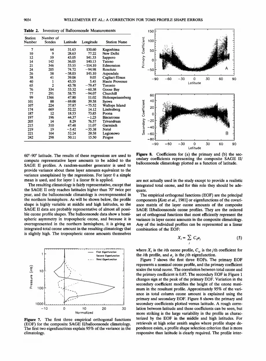
Figure 8. Coefficients for (a) the primary and (b) the secondary coefficients representing the composite SAGE II/ balloonsonde climatology plotted as a function of latitude.

are not actually used in the study except to provide a realistic integrated total ozone, and for this role they should be ade- quate.

The empirical orthogonal functions (EOF) are the principal components [Kotz et al., 1981] or eigenfunctions of the covari- ance matrix of the layer ozone amounts of the composite SAGE II/balloonsonde ozone profiles. They are the ordered set of orthogonal functions that most efficiently represent the variance in layer ozone amounts in the composite climatology. Any of the individual profiles can be represented as a linear combination of the EOF:

Xi-- • Cija j (5) J

where X• is the ith ozone profile, C o is the jth coefficient for the i th profile, and a• is the j th eigenfunction.

Figure 7 shows the first three EOFs. The primary EOF represents a nominal ozone profile, and the primary coefficient scales the total ozone. The correlation between total ozone and

the primary coefficient is 0.87. The secondary EOF in Figure 1 changes sign at the peak of the primary EOF. Variation in the secondary coefficient modifies the height of the ozone maximum in the resultant profile. Approximately 95% of the variance in total column ozone amount is explained using the primary and secondary EOF. Figure 8 shows the primary and secondary coefficients plotted versus latitude. A rough correlation between latitude and these coefficients can be seen, but more striking is the large variability in the profile as characterized by the EOF in the middle and high latitudes. For retrievals at high solar zenith angles where profile shape dependence exists, a profile shape selection criterion that is more responsive than latitude is clearly required. The profile inter-


polation procedure described in the previous section provides this capability, but to reduce the need for extrapolation in this procedure, standard profiles which better span the set of possible profiles are needed.

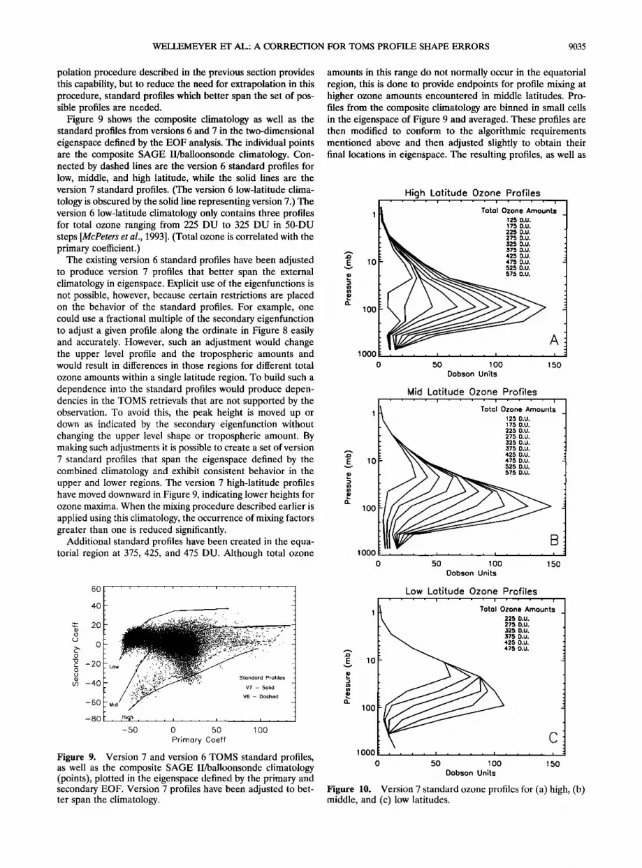
Figure 9 shows the composite climatology as well as the standard profiles from versions 6 and 7 in the two-dimensional eigenspace defined by the EOF analysis. The individual points are the composite SAGE II/balloonsonde climatology. Con- nected by dashed lines are the version 6 standard profiles for low, middle, and high latitude, while the solid lines are the version 7 standard profiles. (The version 6 low-latitude climatology is obscured by the solid line representing version 7.) The version 6 low-latitude climatology only contains three profiles for total ozone ranging from 225 DU to 325 DU in 50-DU steps [McPeters et al., 1993]. (Total ozone is correlated with the primary coetticient.)

The existing version 6 standard profiles have been adjusted to produce version 7 profiles that better span the external climatology in eigenspace. Explicit use of the eigenfunctions is not possible, however, because certain restrictions are placed on the behavior of the standard profiles. For example, one could use a fractional multiple of the secondary eigenfunction to adjust a given profile along the ordinate in Figure 8 easily and accurately. However, such an adjustment would change the upper level profile and the tropospheric amounts and would result in differences in those regions for different total ozone amounts within a single latitude region. To build such a dependence into the standard profiles would produce depen- dencies in the TOMS retrievals that are not supported by the observation. To avoid this, the peak height is moved up or down as indicated by the secondary eigenfunction without changing the upper level shape or tropospheric amount. By making such adjustments it is possible to create a set of version 7 standard profiles that span the eigenspace defined by the combined climatology and exhibit consistent behavior in the upper and lower regions. The version 7 high-latitude profiles have moved downward in Figure 9, indicating lower heights for ozone maxima. When the mixing procedure described earlier is applied using this climatology, the occurrence of mixing factors greater than one is reduced significantly.

Additional standard profiles have been created in the equatorial region at 375, 425, and 475 DU. Although total ozone

amounts in this range do not normally occur in the equatorial region, this is done to provide endpoints for profile mixing at higher ozone amounts encountered in middle latitudes. Pro- files from the composite climatology are binned in small cells in the eigenspace of Figure 9 and averaged. These profiles are then modified to conform to the algorithmic requirements mentioned above and then adjusted slightly to obtain their final locations in eigenspace. The resulting profiles, as well as

ß ,

1

10

100

1000 - . .

o

High Latitude Ozone Profiles ß , i .... i .... i

Totol Ozone Amounts 125 O.U. 175 D.U. 225 D.U. 275 D.U. 325 D.U. 37õ D.U. 425 D.U. 475 D.U. 525 D.U. 575 D.U.

ß . i .... i

50 1 O0

Dobson Units

A

150

1

10

lOO

1 ooo

o

Mid Latitude Ozone Profiles

Total Ozone Amounts 125 D.u.

• 175 D.U. X 225 D.U. •,. 275 D.U. • 325 D.U.

'•N'• 575 D.U. •'• 425 D.U.

•'• •. 475 D.U. \ \ •'•,,• 525 D.U.

ß ß , i i , , i i i , , , , i

50 1 O0 150 Dobson Units

60 f ' ' ] ' t i ' ' ' 40

ß .• ' '.•,-"--•-?,' ' .•-•-1,.%'.:'i:,.'.': .•>'.:.:./,:.:'•'.: 4,,....-.'. ß - .'.- :....,. /

o o ,ow .:½ii:•.•?t ..... :5'-'"'; ';"'5..• ...... ,

g -20 g Stondord Profiles f.D -- 40 .:?...,;5i•.•:i?'•:? }:': ' :' ":;"?' ?'"' V7 - Solid

"11 ?:5!'""•:%5'15 V6 - Dashed --60 Mid ....

--80 , ,Higth .... I .... I .... I , , ,

-5O 0 50 100

Primary Coeff

Figure 9. Version ? and version 6 TOMS standard profiles, as well as the composite SAGE II/balloonsonde climatology (points), plotted in the eigenspace defined by the primary and secondary EOF. Version ? profiles have been adjusted to better span the climatology.

10

100

1000 ß . ........ •

0 .50 100

Low Latitude Ozone Profiles ' ' i .... i .... i

Total Ozone Amounts 225 D.U. 275 D.U. 525 D.U. 375 D.U. 425 D.U. 475 D.U.

150

Dobson Units

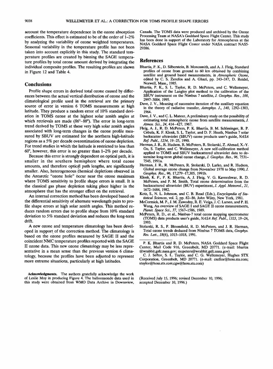
Figure 10. Version 7 standard ozone profiles for (a) high, (b) middle, and (c) low latitudes.


0.1

1.0

10.0

100.0

1000.0 ,

-1.0

I , , , • I , , , , 1

-0.5 0.0 0.5

Correlation Coefficient

Figure 11. Vertical profile of correlation between layer temperature and total ozone amount. SAGE II coincident Na- tional Meteorological Center temperatures are correlated with the integrated total ozone from individual profiles in the composite SAGE II/balloonsonde climatology.

the rest of the version 7 ozone profiles, are shown in Figure 10 and Table 3.

We note that the interpolation procedure described in the previous section does not take place in the eigenspace illustrated in Figure 9. It is a two-dimensional interpolation done by interpolation along the separate climatologies (connected by solid lines in Figure 9) which vary in total ozone and between two of the climatologies which vary in height of the ozone maximum. These coordinates are not necessarily orthogonal, though they are seen to be roughly so by examination of the primary and secondary EOF in Figure 7. As discussed in the previous section, the interpolation is limited to two dimen- sions by availability of information.

The tropospheric ozone amounts from the balloonsonde climatology exhibit a hemispheric asymmetry. The possibility of using separate sets of standard profiles in the two hemi- spheres is rejected, however, because the impact of the tropospheric ozone on the total ozone retrieval is minimal. The tropospheric ozone amount represents only 3% of the total column amount and is partly measured by TOMS [Klenk et al., 1982]. Building in a small hemispheric asymmetry based on external data sources is probably an unwarranted complication to the TOMS retrieval and the interpretation of the TOMS data. The use of symmetric tropospheres in the retrieval results in small errors that are more easily interpreted by the user. A small concession to the asymmetry is made, however, by using lower tropospheric amounts in the case of the 125- and 175-DU profiles because they are only found in the southern hemisphere. A somewhat smaller tropospheric amount is also used in the 225-DU profile. If total ozone amounts of this magnitude are' encountered in the northern hemisphere, a small error will result [Klenk et al., 1982].

10

lOO

1 ooo

1 -

High Latitude Temperature Profiles

Total Ozone Amounts _ 125 D.U. 175 D.U. 22,5 D.U.

27,5 - ,57,5 D.U.

.

125 D.U. D.U.

A , I , i , I , , , I ß ß ß i . . . i I ' ' I ' i ' i . . .

160 180 200 220 240 260 280 .300 Kelvin

10

lOO

1 ooo

Mid Lotitude Temperoture Profiles ß i ß ß ß I ß ' ß i ß ß ß i ß ß ß i ß ß ß i ß ß ß I ß ß ß

Total Ozone Amounts I - 125 D.U. 175 D.U. 225 D.U. 275 D.U. 325 D.U. 375 D.U. 425 D.U. 475 D.U. 525 D.U. 575 D.U.

125 D.U.

B , I i , , I . . ß i . . . i . . . i . . I I ' I ß I" '"

160 180 200 220 240 260 280 .300 Kelvin

10

100

1000

Low Latitude Temperature Profiles ß i ß ß ß i ' ' ß i ' ß ß i ß ' ß I ' ' ß i ß ' ' I ' ' ß

Total Ozone Amounts / - 225 D.U. 275 D.U. 325 D.U. 375 D.U. 425 D.U. 475 D.U.

225 D.U. 475 D.U.

c ß i , . o i , , , i , . , i , , ß i ß . , i o , , i , , .

160 180 200 220 240 260 280 .300

Kelvin

Figure 12. Version 7 standard temperature profiles for (a) high, (b) middle, and (c) low latitudes.

New Climatological Temperature Profiles The climatological temperature profiles have also been re-

computed for use in the version 7 algorithm. Coincident NMC temperature profiles are reported with the SAGE II ozone profiles [McCormick et al., 1989]. The temperature of the layer center determined in units of the logarithm of pressure is used to represent each Umkehr layer. These temperatures have been averaged by total ozone amount in the three separate

latitude regions in order to give a separate climatological temperature profile for each ozone profile. These results are quite similar to the version 6 climatology except for the total ozone dependence in the vicinity of the ozone maximum. Figure 11 shows a profile of layer temperature correlation with total ozone indicating a maximum of about 0.5 near the ozone maximum. Because of this, the total ozone dependent temperature profiles have been adopted in version 7 to take into


Table 3. TOMS Version 7 Standard Ozone Profiles

Umkehr Layer

Profile 0 1 2 3 4 5 6 7 8 9 >9

Low latitude 225 15.0 9.0 5.0 7.0 25.0 62.2 57.0 29.4 10.9 3.2 1.3 275 15.0 9.0 6.0 12.0 52.0 79.2 57.0 29.4 10.9 3.2 1.3 325 15.0 9.0 10.0 31.0 71.0 87.2 57.0 29.4 10.9 3.2 1.3 375 15.0 9.0 21.0 53.0 88.0 87.2 57.0 29.4 10.9 3.2 1.3 425 15.0 9.0 37.0 81.0 94.0 87.2 57.0 29.4 10.9 3.2 1.3 475 15.0 9.0 54.0 108.0 100.0 87.2 57.0 29.4 10.9 3.2 1.3

Middle latitude 125 6.0 5.0 4.0 6.0 8.0 31.8 28.0 20.0 11.1 3.7 1.4 175 8.0 7.0 8.0 12.0 26.0 41.9 33.6 22.3 11.1 3.7 1.4 225 10.0 9.0 12.0 18.0 44.0 52.1 39.2 24.5 11.1 3.7 1.4 275 16.0 12.0 15.0 29.0 58.0 63.7 40.6 24.5 11.1 3.7 1.4 325 16.0 14.0 26.0 45.0 74.7 66.9 41.7 24.5 11.1 3.7 1.4 375 16.0 16.0 39.0 64.0 85.7 71.1 42.5 24.5 11.1 3.7 1.4 425 16.0 18.0 54.0 84.0 97.7 71.7 42.9 24.5 11.1 3.7 1.4 475 16.0 22.0 72.0 107.7 101.0 72.6 43.0 24.5 11.1 3.7 1.4 525 16.0 26.0 91.0 127.7 108.0 72.6 43.0 24.5 11.1 3.7 1.4 575 16.0 30.0 110.0 147.7 115.0 72.6 43.0 24.5 11.1 3.7 1.4

High latitude 125 9.5 7.0 18.3 7.6 8.2 28.6 22.0 12.4 7.7 2.5 1.2 175 9.5 8.0 22.8 22.0 26.9 32.3 26.8 15.0 8.0 2.5 1.2 225 10.0 9.0 27.6 45.7 41.0 35.0 28.8 15.4 8.3 2.9 1.3 275 14.0 12.0 34.0 66.9 54.2 36.0 28.8 15.4 8.9 3.4 1.4 325 14.0 15.0 46.8 82.6 65.2 41.7 28.8 17.2 8.9 3.4 1.4 375 14.0 20.0 61.2 93.8 75.2 45.9 32.5 18.7 8.9 3.4 1.4 425 14.0 25.0 76.2 104.9 84.2 51.4 35.6 20.0 8.9 3.4 1.4 475 14.0 32.0 91.0 117.1 93.0 55.8 37.5 20.9 8.9 3.4 1.4 525 14.0 41.0 107.1 128.1 101.0 60.2 38.2 21.7 8.9 3.4 1.4 575 14.0 49.0 123.2 142.2 111.0 60.6 38.8 22.5 8.9 3.4 1.4

Values are in Dobson units.

Table 4. TOMS Version 7 Standard Temperature Profiles

Umkehr Layer

Profile 0 1 2 3 4 5 6 7 8 9 >9

Low latitude 225 283.0 251.0 215.6 200.7 210.7 221.6 231.1 245.3 258.7 267.4 265.4 275 283.0 251.0 215.9 203.5 211.9 222.5 231.1 245.3 258.7 267.4 265.4 325 283.0 251.0 216.5 207.0 213.6 223.0 231.1 245.3 258.7 267.4 265.4 375 283.0 251.0 216.0 210.0 216.0 224.0 231.1 245.3 258.7 267.4 265.4 425 283.0 251.0 216.0 213.0 217.0 224.5 231.1 245.3 258.7 267.4 265.4 475 283.0 251.0 216.0 216.0 219.0 225.0 231.1 245.3 258.7 267.4 265.4

Middle latitude 125 237.0 218.0 196.0 191.0 193.0 210.0 227.6 239.4 253.6 263.9 262.6 175 260.0 228.0 201.7 198.0 202.1 214.3 227.6 239.4 253.6 263.9 262.6 225 273.0 239.0 213.3 207.5 211.7 219.1 227.6 239.4 253.6 263.9 262.6 275 273.0 239.0 217.1 212.2 214.9 220.4 227.6 239.4 253.6 263.9 262.6 325 273.0 239.0 219.1 216.6 217.0 220.8 227.6 239.4 253.6 263.9 262.6 375 273.0 239.0 220.2 219.0 219.0 221.9 227.6 239.4 253.6 263.9 262.6 425 273.0 239.0 220.9 220.7 221.0 223.7 227.6 239.4 253.6 263.9 262.6 475 273.0 239.0 221.5 222.5 222.7 224.4 227.6 239.4 253.6 263.9 262.6 525 273.0 239.0 222.3 224.8 225.5 225.8 227.6 239.4 253.6 263.9 262.6 575 273.0 239.0 225.0 227.0 227.0 227.0 227.6 239.4 253.5 263.9 262.6

High latitude 125 237.0 218.0 196.0 191.0 193.0 210.0 223.3 237.1 251.6 262.4 265.6 175 260.0 228.0 201.7 198.0 202.1 214.3 223.3 237.1 251.6 262.4 265.6 225 260.0 228.0 209.7 208.5 212.5 222.0 228.0 237.1 251.6 262.4 265.6 275 260.0 228.0 222.6 223.4 223.8 226.5 231.6 237.1 251.6 262.4 265.6 325 260.0 228.0 222.6 223.4 223.8 226.5 231.6 237.1 251.5 262.4 265.6 375 260.0 228.0 222.6 223.4 223.8 226.5 231.6 237.1 251.5 262.4 265.6 425 260.0 228.0 222.6 223.4 223.8 226.5 231.6 237.1 251.5 262.4 265.6 475 260.0 228.0 222.6 223.4 223.8 226.5 231.6 237.1 251.5 262.4 265.6 525 260.0 228.0 222.6 223.4 223.8 226.5 231.6 237.1 251.5 262.4 265.6 575 260.0 228.0 222.6 223.4 223.8 226.5 231.6 237.1 251.5 262.4 265.6

Values are in Dobson units.


account the temperature dependence in the ozone absorption coefficients. This effect is estimated to be of the order of 1-2%

by analyzing the variability of ozone weighted temperatures. Seasonal variability in the temperature profile has not been taken into account explicitly in this study. The standard temperature profiles are created by binning the SAGE temperature profiles by total ozone amount derived by integrating the individual composite profiles. The resulting profiles are shown in Figure 12 and Table 4.

Conclusions

Profile shape errors in derived total ozone caused by differences between the actual vertical distribution of ozone and the

climatological profile used in the retrieval are the primary source of error in version 6 TOMS measurements at high latitude. They produce a random error of 10% standard deviation in TOMS ozone at the highest solar zenith angles at which retrievals are made (86ø-88ø). The error in long-term trend derived by TOMS at these very high solar zenith angles associated with long-term changes in the ozone profile measured by SBUV are estimated for the northern high-latitude regions as a 5 % per decade overestimation of ozone depletion. For trend studies in which the latitude is restricted to less than

60 ø , however, this error is no greater than 1-2% per decade. Because this error is strongly dependent on optical path, it is

smaller in the southern hemisphere where total ozone amounts, and therefore optical path lengths, are significantly smaller. Also, heterogeneous chemical depletions observed in the Antarctic "ozone hole" Occur near the ozone maximum

where TOMS sensitivity to •rofile shape errors is small. It is the classical gas phase depletion taking place higher in the atmosphere that has the stronger effect on the retrieval.

An internal correction method has been developed based on the differential sensitivity of alternate wavelength pairs to profile shape errors at high solar zenith angles. This method reduces random errors due to profile shape from 10% standard deviation to 5% standard deviation and reduces the long-term drift.

A new ozone and temperature climatology has been developed in support of the correction method. The climatology is based on the ozone profiles measured by SAGE II and the coincident NMC temperature profiles reported with the SAGE II ozone data. This new ozone climatology may be less representative in a mean sense than the previous version 6 climatology, because the profiles have been adjusted to represent more extreme situations, particularly at high latitudes.

Canada. The TOMS data were produced and archived by the Ozone Processing Team at NASA's Goddard Space Flight Center. This study has been done in support of the Laboratory for Atmospheres at the NASA Goddard Space Flight Center under NASA contract NAS5- 29386.

References

Bhartia, P. K., D. Silberstein, B. Monosmith, and A. J. Fleig, Standard profiles of ozone from ground to 60 km obtained by combining satellite and ground based measurements, in Atmospheric Ozone, edited by C. S. Zerefos and A. Ghazi, pp. 243-247, D. Reidel, Norwell, Mass., 1985.

Bhartia, P. K., S. L. Taylor, R. D. McPeters, and C. Wellemeyer, Application of the Langley plot method to the calibration of the SBUV instrument on the Nimbus 7 satellite, J. Geophys. Res., 100, 2997-3004, 1995.

Dave, J. V., Meaning of successive iteration of the auxiliary equation in the theory of radiative transfer, Astrophys. J., 140, 1292-1303, 1964.

Dave, J. V., and C. L. Mateer, A preliminary study on the possibility of estimating total atmospheric ozone from satellite measurements, J. Atmos. Sci., 24, 414-427, 1967.

Fleig, A. J., R. D. McPeters, P. K. Bharfia, B. M. Schlesinger, R. P. Cebula, K. F. Klenk, S. L. Taylor, and D. F. Heath, Nimbus 7 solar backscatter ultraviolet (SBUV) ozone products user's guide, NASA Ref. Publ., 1234, 19-25, 1990.

Herman, J. R., R. Hudson, R. McPeters, R. Stolarski, Z. Ahmad, X.-Y. Gu, S. Taylor, and C. Wellemeyer, A new self-calibration method applied to TOMS and SBUV backscattered ultraviolet data to determine long-term global ozone change, J. Geophys. Res., 96, 7531- 7545, 1991a.

Herman, J. R., R. McPeters, R. Stolarski, D. Larko, and R. Hudson, Global average ozone change from November 1978 to May 1990, J. Geophys. Res., 96, 17,279-17,305, 1991b.

Klenk, K. F., P. K. Bhartia, A. J. Fleig, V. G. Kaveeshwar, R. D. McPeters, and P.M. Smith, Total ozone determination from the backscattered ultraviolet (BUV) experiment, J. Appl. Meteorol., 21, 1672-1684, 1982.

Kotz, S., N. L. Johnson, and C. B. Read (Eds.), Encyclopedia of Sta- tistical Sciences, vol. 2, pp. 82-86, John Wiley, New York, 1981.

McCormick, M.P., J. M. Zawodny, R. E. Veiga, J. C. Larsen, and P. H. Wang, An overview of SAGE I and SAGE II ozone measurements, Planet. Space Sci., 37, 1567-1586, 1989.

McPeters, R. D., et al., Nimbus-7 total ozone mapping spectrometer (TOMS) data products user's guide, NASA Ref. Publ., 1323, 19-24, 1993.

Stolarski, R. S., P. Bloomfield, R. D. McPeters, and J. R. Herman, Total ozone trends deduced from Nimbus 7 TOMS data, Geophys. Re•. Lett., 18(6), 1015-1018, 1991.

P. K. Bhartia and R. D. McPeters, NASA Goddard Space Flight Center, Mail Code 916, Greenbelt, MD 20771. (e-mail: bhartia @wrabbit.gsfc.nasa.gov; mcpeters@wrabbit'gsfc'nasa'gøv)

C: J. Seftor, S. L. Taylor, and C. G. Wellemeyer, Hughes STX Corporation, Greenbelt, MD 20771. (e-mail: [email protected]. com; staylør@høss'stx'cøm;cgw@høss'stx'cøm)

Acknowledgments. The authors gratefully acknowledge the wdrk of Leslie Moy in producing Figure 4. The balloonsonde data used in this study were obtained from WMO Data Archive in Downsview,

(Received July 15, 1996; revised December 10, 1996; accepted December 10, 1996.)

a correction for total ozone mapping spectrometer profile shape errors at high latitude

Documents