3c duct design method

3C DUCT DESIGN METHOD

Huan-Ruei Shiu * Feng-Chu Ou " Sih-Li Chen "

Department of Mechanical EngineeringNational Taiwan University

Taipei, Taiwan 10617, R.O.C.

ABSTRACT

A new 3C duct design method is proposed for designing a high quality, energy-efficiencycost-effective air duct system. It not only considers the demand of volume flow rate, but also takesinto consideration a number of issues including system pressure balance, noise, vibration, spacelimitation and total system cost. This new method comprises three major calculation procedures:initial computer-aided design (CAD), computer-aided simulation (CAS) and correction processes (CP).An example is presented in this study to understand the characteristics of 3C method. It shows that 3Cduct design method provides a simple computation procedure for an optimum air duct system. It alsoshortens the design schedule, prevents human calculation errors, and reduces the dependence ondesigner experience. In addition to apply in a new duct system design, 3C duct design method is alsoa powerful design tool for the expansion of an existing duct system.

Keywords : 3C duct design method, Semiconductor factory, Exhaust system, HVAC.

1. INTRODUCTION

Duct design is important for commercial, industrial,and residential air duct systems. An optimum air ductsystem transports the required amount of conditioned,recirculated, or exhausted air to the specific space andmeets the following requirements: (1)an optimum ductsystem layout within the allocated space, (2) asatisfactory system pressure balance, (3) space noiselevel lower than the allowable limits, and (4) optimumenergy cost and initial cost. Deficiencies in ductdesign can result in systems that operate incorrectly andincrease the initial or running cost.

Most conventional Heating, Ventilating, and Air-Conditioning (HVAC) duct design methods consist ofequal velocity, equal friction, balanced capacity(pressure), and static regain. The equal velocitymethod or the equal friction method may be simple, butthey fail to achieve pressure balance. Thus, the systemdesigned does not meet the actual operations. On-siteventilation adjustment after project completion becomesnecessary. In some cases, large fans must be installedto make up for poor designs, which add to extra cost.Shieh [1] improved the static regain method to simplifythe calculation procedures and ensure the advantage ofsystem pressure balance. However it does not containthe cost concept, like other conventional design method,and thus cannot meet the optimization requirement.

T-method proposed by Tsal, et al., [2~4] is the most

comprehensive and powerful tool applied in duct design.It uses iteration computation and cost optimizationtheory, which enable the designed system to have thelowest life cycle cost and all paths to have the samepressure loss. There is no need to waste extra time ormoney to attain system pressure balance. However,T-method offers poor control of flow velocity or ductdiameter. In cases of relatively inexpensive initial cost,the flow velocity may be too high. In contrast, forcases of relatively inexpensive energy cost, the duct sizemay be too big. Nevertheless, in actual duct design,considerations of the factors of space and noise oftenrequire the limit on the duct diameter or flow velocityduring certain sections. When there are too manylimitations, it is difficult to obtain the satisfactoryoptimal solution from T-method. Thus, a new 3Cdesign method, which is suitable for the duct systemdesign, is proposed in this paper.

2. 3C DUCT DESIGN METHOD

For a complete duct design case, one should providethe information on the given design conditions andlimitations. Given design conditions and limitationsregarding the duct system include (1)basic information:such as duct system layout, liquid physical property andduct materials; (2)system requirements: such as volumeflow rate, length and cross section shape; (3) duct

* Graduate student ** Professor

The Chinese Journal of Mechanics-Series A, Vol. 18, No. 2, June 2002 67

Dow

nloaded from https://academ

ic.oup.com/jom

/article/18/2/67/5934268 by guest on 25 March 2022

information: such as the loss coefficient of variousaccessories and equipments [5,6]; (4) safety concerns:such as the minimum velocity for safety [7] or themaximum velocity to prevent vibrations and noise [8];(5) cost concern: such as total duct surface area or thevolume flow rate and performance of the fan.

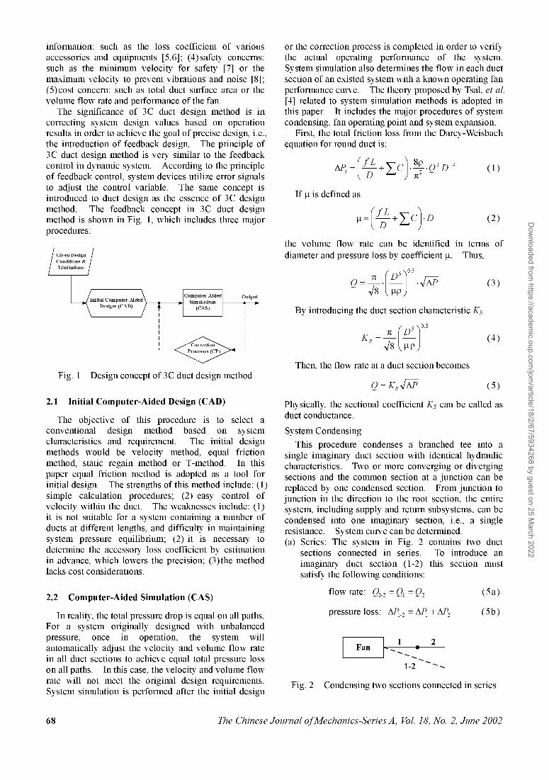
The significance of 3C duct design method is incorrecting system design values based on operationresults in order to achieve the goal of precise design, i.e.,the introduction of feedback design. The principle of3C duct design method is very similar to the feedbackcontrol in dynamic system. According to the principleof feedback control, system devices utilize error signalsto adjust the control variable. The same concept isintroduced to duct design as the essence of 3C designmethod. The feedback concept in 3C duct designmethod is shown in Fig. 1, which includes three majorprocedures:

Output

Fig. 1 Design concept of 3C duct design method

2.1 Initial Computer-Aided Design (CAD)

The objective of this procedure is to select aconventional design method based on systemcharacteristics and requirement. The initial designmethods would be velocity method, equal frictionmethod, static regain method or T-method. In thispaper equal friction method is adopted as a tool forinitial design. The strengths of this method include: (1)simple calculation procedures; (2) easy control ofvelocity within the duct. The weaknesses include: (1)it is not suitable for a system containing a number ofducts at different lengths, and difficulty in maintainingsystem pressure equilibrium; (2) it is necessary todetermine the accessory loss coefficient by estimationin advance, which lowers the precision; (3)the methodlacks cost considerations.

2.2 Computer-Aided Simulation (CAS)

In reality, the total pressure drop is equal on all paths.For a system originally designed with unbalancedpressure, once in operation, the system willautomatically adjust the velocity and volume flow ratein all duct sections to achieve equal total pressure losson all paths. In this case, the velocity and volume flowrate will not meet the original design requirements.System simulation is performed after the initial design

or the correction process is completed in order to verifythe actual operating performance of the system.System simulation also determines the flow in each ductsection of an existed system with a known operating fanperformance curve. The theory proposed by Tsal, et al.[4] related to system simulation methods is adopted inthis paper. It includes the major procedures of systemcondensing, fan operating point and system expansion.

First, the total friction loss from the Darcy-Weisbachequation for round duct is:

D

If (x is defined as

(1)

(2)

By introducing the duct section characteristic KS

y-v.

Then, the flow rate at a duct section becomes

the volume flow rate can be identified in terms ofdiameter and pressure loss by coefficient \i. Thus,

(3)

(4)

(5)

Physically, the sectional coefficient KS can be called asduct conductance.

System Condensing

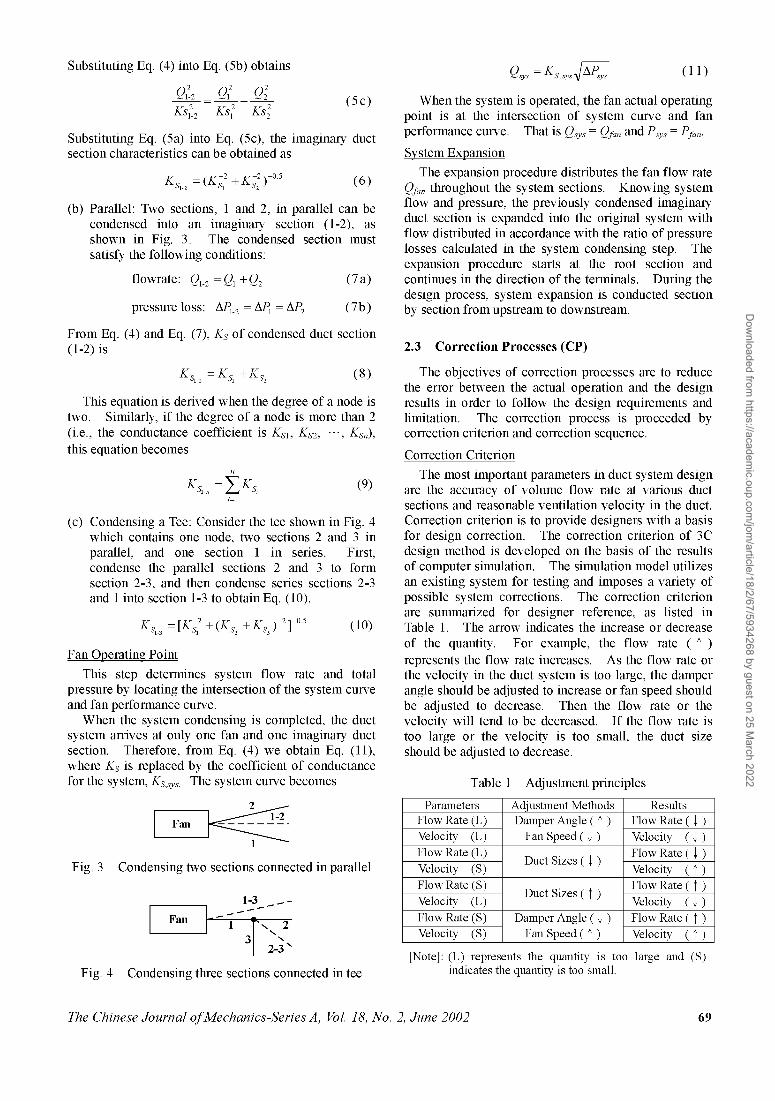
This procedure condenses a branched tee into asingle imaginary duct section with identical hydrauliccharacteristics. Two or more converging or divergingsections and the common section at a junction can bereplaced by one condensed section. From junction tojunction in the direction to the root section, the entiresystem, including supply and return subsystems, can becondensed into one imaginary section, i.e., a singleresistance. System curve can be determined.(a) Series: The system in Fig. 2 contains two duct

sections connected in series. To introduce animaginary duct section (1-2) this section mustsatisfy the following conditions:

flow rate: Q1-2=Q1=Q2

pressure loss: APU2 = APl + AP2

(5a)

(5b)

Fan

1-2

Fig. 2 Condensing two sections connected in series

68 The Chinese Journal of Mechanics-Series A, Vol. 18, No. 2, June 2002

Dow


ic.oup.com/jom


Substituting Eq. (4) into Eq. (5b) obtains

Qi-2 _ Q1 2 Q2Ks2 Ks2 + Ks2

(5c)

Substituting Eq. (5a) into Eq. (5c), the imaginary ductsection characteristics can be obtained as

) (6)

(b) Parallel: Two sections, 1 and 2, in parallel can becondensed into an imaginary section (1-2), asshown in Fig. 3. The condensed section mustsatisfy the following conditions:

flowrate: Q1-2=Q1+Q2

pressure loss: ^ = APl = AP2

(7a)

(7b)

From Eq. (4) and Eq. (7), KS of condensed duct section(1-2) is

(8)

This equation is derived when the degree of a node istwo. Similarly, if the degree of a node is more than 2(i.e., the conductance coefficient is KS1, KS2, •••, KSn),this equation becomes

(9)

(c) Condensing a Tee: Consider the tee shown in Fig. 4which contains one node, two sections 2 and 3 inparallel, and one section 1 in series. First,condense the parallel sections 2 and 3 to formsection 2-3, and then condense series sections 2-3and 1 into section 1-3 to obtain Eq. (10).

A-̂ = [A.£ -\-yK<< -\-Ktj ) J (10)

Fan Operating Point

This step determines system flow rate and totalpressure by locating the intersection of the system curveand fan performance curve.

When the system condensing is completed, the ductsystem arrives at only one fan and one imaginary ductsection. Therefore, from Eq. (4) we obtain Eq. (11),where KS is replaced by the coefficient of conductancefor the system, KS,sys. The system curve becomes

Fan

Fig. 3 Condensing two sections connected in parallel

Fan1

1-3-~ — ~~

3. 2

2-3 N

(11)

When the system is operated, the fan actual operatingpoint is at the intersection of system curve and fanperformance curve. That is Qsys = Qfan and Psys = Pfan.

System Expansion

The expansion procedure distributes the fan flow rateQfan throughout the system sections. Knowing systemflow and pressure, the previously condensed imaginaryduct section is expanded into the original system withflow distributed in accordance with the ratio of pressurelosses calculated in the system condensing step. Theexpansion procedure starts at the root section andcontinues in the direction of the terminals. During thedesign process, system expansion is conducted sectionby section from upstream to downstream.

2.3 Correction Processes (CP)

The objectives of correction processes are to reducethe error between the actual operation and the designresults in order to follow the design requirements andlimitation. The correction process is proceeded bycorrection criterion and correction sequence.

Correction Criterion

The most important parameters in duct system designare the accuracy of volume flow rate at various ductsections and reasonable ventilation velocity in the duct.Correction criterion is to provide designers with a basisfor design correction. The correction criterion of 3Cdesign method is developed on the basis of the resultsof computer simulation. The simulation model utilizesan existing system for testing and imposes a variety ofpossible system corrections. The correction criterionare summarized for designer reference, as listed inTable 1. The arrow indicates the increase or decreaseof the quantity. For example, the flow rate ( f )represents the flow rate increases. As the flow rate orthe velocity in the duct system is too large, the damperangle should be adjusted to increase or fan speed shouldbe adjusted to decrease. Then the flow rate or thevelocity will tend to be decreased. If the flow rate istoo large or the velocity is too small, the duct sizeshould be adjusted to decrease.

Table 1 Adjustment principles

ParametersFlow Rate (L)Velocity (L)Flow Rate (L)Velocity (S)Flow Rate (S)Velocity (L)Flow Rate (S)Velocity (S)

Adjustment MethodsDamper Angle ( f )

Fan Speed ( I )

Duct Sizes ( I )

Duct Sizes ( f )

Damper Angle ( I )Fan Speed ( f )

ResultsFlow Rate ( I )Velocity ( I )Flow Rate ( I )Velocity ( f )Flow Rate ( f )Velocity ( I )Flow Rate ( f )Velocity ( f )

Fig. 4 Condensing three sections connected in tee[Note]: (L) represents the quantity is too large and (S)

indicates the quantity is too small.


Dow


ic.oup.com/jom


Correction Sequence

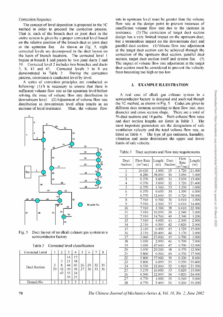
The concept of level deposition is proposed in the 3Cmethod in order to proceed the correction process.That is, each of the branch duct or joint duct in theentire system is given by a proper corrected level basedon the relative position of the branch duct or joint ductto the upstream fan. As shown in Fig. 5, eightcorrected levels are decomposed in the duct layout onthe basis of branch locations. The corrected level 1begins at branch 1 and passes by two joint ducts 2 and39. Corrected level 2 includes two branches and ducts3, 8, 42 and 43. Corrected levels 3 to 8 aredemonstrated in Table 2. During the correctionprocess, correction is conducted level by level.

A series of correction principles are conducted asfollowing: (1) It is necessary to ensure that there issufficient volume flow rate in the upstream level beforesolving the issue of volume flow rate distribution indownstream level. (2) Adjustment of volume flow ratedistribution in downstream level often results in anincrease of local resistance. Thus, the volume flow

Branch No.

Fig. 5 Duct layout of an alkali exhaust gas system in asemiconductor factory

Table 2 Corrected level classification

Corrected Level

Duct Section

Branch No.

1

239

1

Is)

38

4243

Is)

3

142144495556

3

4

171845482425

3

5

2627

1

6

2930

1

7

3233

1

8

3536

1

rate in upstream level must be greater than the volumeflow rate at the design point to prevent instances ofinsufficient volume flow rate due to the increase inresistance. (3) The correction of target duct sectiondesign has a very limited impact on the upstream duct,but a tremendous impact on the downstream duct andparallel duct section. (4) Volume flow rate adjustmentat the target duct section can be achieved through thecorrection of the upstream duct section, parallel ductsection, target duct section itself and system fan. (5)The impact of volume flow rate adjustment at the targetduct section must be considered to prevent the velocityfrom becoming too high or too low.

3. EXAMPLE ILLUSTRATION

A real case of alkali gas exhaust system in asemiconductor factory is designed and analyzed thoughthe 3C method, as shown in Fig. 5. Codes are given todifferent duct sections according to their flow rate, ductdiameter and cross section shape. There are a total of56 duct sections and 14 paths. Both exhaust flow ratesand duct section lengths are listed in Table 3. Themost important parameters are the designation of safeventilation velocity and the total volume flow rate, aslisted in Table 4. The type of gas emission, humidity,vibration and noise determines the upper and lowerlimits of safe velocity.

Table 3

DuctSection

1

Is)

345678910111213141516171819202122232425262728

Duct sections and

Flow Rate(m3/sec)

10.6208.2800.3700.3700.3700.3700.3707.9107.9107.9107.9107.9107.9102.1102.1102.1101.0601.0501.0501.0505.8005.8005.8000.5305.2700.5004.7704.770

Length(m)

1.00038.000

3.8003.0001.5009.600

12.6000.5002.5004.500

10.50014.7004.0000.5006.400

20.40023.000

2.00047.60020.200

0.50057.0006.000

22.00016.00022.000

1.0005.400

flow rate requirements

DuctSection

29303132333435363738394041424344454647484950515253545556

FlowRate

(m3/sec)1.7203.0503.0501.7201.3301.3300.7200.6100.6100.6102.3402.3402.3400.8201.5201.1700.7000.7000.7000.4700.3300.3300.3300.8200.8200.8200.5600.260

Length(m)

21.4001.000

13.40021.400

1.0006.000

18.0001.000

14.40022.400

1.0003.2002.0002.000

15.0003.0001.0007.000

12.00012.00017.5008.600

10.40021.50015.00024.000

5.00010.200


Dow


ic.oup.com/jom


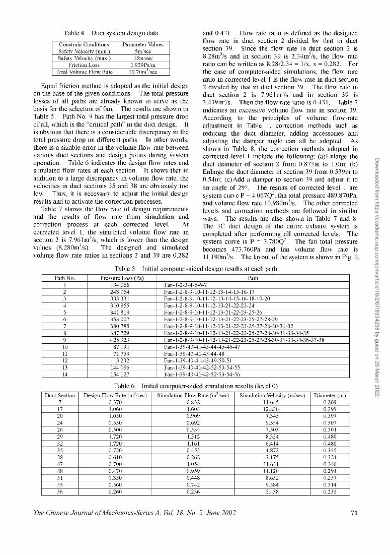
Table 4 Duct system design data

Constrain ConditionsSafety Velocity (min.)Safety Velocity (max.)

Friction LossTotal Volume Flow Rate

Parameter Values5m/sec15m/sec

1.929Pa/m10.70m3/sec

Equal friction method is adopted as the initial designon the base of the given conditions. The total pressurelosses of all paths are already known to serve as thebasis for the selection of fan. The results are shown inTable 5. Path No. 9 has the largest total pressure dropof all, which is the "critical path" in the duct design. Itis obvious that there is a considerable discrepancy in thetotal pressure drop on different paths. In other words,there is a sizable error in the volume flow rate betweenvarious duct sections and design points during systemoperation. Table 6 indicates the design flow rates andsimulated flow rates at each section. It shows that inaddition to a large discrepancy in volume flow rate, thevelocities in duct sections 35 and 38 are obviously toolow. Thus, it is necessary to adjust the initial designresults and to activate the correction processes.

Table 7 shows the flow rate of design requirementsand the results of flow rate from simulation andcorrection process at each corrected level. Atcorrected level 1, the simulated volume flow rate insection 2 is 7.961m3/s, which is lower than the designvalues (8.280m3/s). The designed and simulatedvolume flow rate ratios in sections 2 and 39 are 0.282

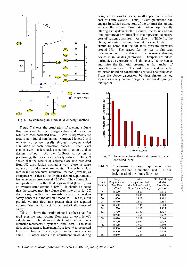
and 0.431. Flow rate ratio is defined as the designedflow rate in duct section 2 divided by that in ductsection 39. Since the flow rate in duct section 2 is8.28m3/s and in section 39 is 2.34m3/s, the flow rateratio can be written as 8.28/2.34 = 1/x, x = 0.282. Forthe case of computer-aided simulations, the flow rateratio in corrected level 1 is the flow rate in duct section2 divided by that in duct section 39. The flow rate induct section 2 is 7.961m3/s and in section 39 is3.439m3/s. Then the flow rate ratio is 0.431. Table 7indicates an excessive volume flow rate in section 39.According to the principles of volume flow-rateadjustment in Table 1, correction methods such asreducing the duct diameter, adding accessories andadjusting the damper angle can all be adopted. Asshown in Table 8, the correction methods adopted incorrected level 1 include the following: (a) Enlarge theduct diameter of section 2 from 0.873m to 1.0m; (b)Enlarge the duct diameter of section 39 from 0.539m to0.54m; (c)Add a damper to section 39 and adjust it toan angle of 29°. The results of corrected level 1 aresystem curve P = 4.067Q2, fan total pressure 489.870Pa,and volume flow rate 10.980m3/s. The other correctedlevels and correction methods are followed in similarways. The results are also shown in Table 7 and 8.The 3C duct design of the entire exhaust system iscompleted after performing all corrected levels. Thesystem curve is P = 3.780Q2. The fan total pressurebecomes 473.760Pa and fan volume flow rate is11.190m3/s. The layout of the system is shown in Fig. 6.

Table 5 Initial computer-aided design results at each path

Path No. Pressure Loss (Pa) Path1 134.066 Fan-1-2-3-4-5-6-7

243.054 Fan-1-2-8-9-10-11-12-13-14-15-16-17333.331 Fan-1-2-8-9-10-11-12-13-14-15-16-18-19-20310.955 Fan-1-2-8-9-10-11-12-13-21-22-23-24341.819 Fan-1-2-8-9-10-11-12-13-21-22-23-25-26353.007 Fan-1-2-8-9-10-11-12-13-21-22-23-25-27-28-29380.785 Fan-1-2-8-9-10-11-12-13-21 -22-23-25-27-28-30-31 -32387.729 Fan-1-2-8-9-10-11-12-13-21-22-23-25-27-28-30-31-33-34-35425.923 Fan-1-2-8-9-10-11-12-13-21-22-23-25-27-28-30-31-33-34-36-37-38

10 87.191 Fan-1-39-40-41-43-44-45-46-4711 71.759 Fan-1-39-40-41-43-44-4812 113.232 Fan-1 -39-40-41-43-49-50-5113 144.096 Fan-1-39-40-41-42-52-53-54-5514 154.127 Fan-1 -39-40-41-42-52-53-54-56

Table 6 Initial computer-aided simulation results (level 0)Duct Section

717202426293235384748515556

Design Flow Rate (m /sec)0.3701.0601.0500.5300.5001.7201.7200.7200.6100.7000.4700.3300.5600.260

Simulation Flow Rate (m /sec)0.8321.6040.9090.6920.5341.5121.1610.4550.2621.0540.9590.4480.7420.236

Simulation Velocity (m/sec)14.64512.8307.3459.3547.5038.3546.4144.8723.175

11.61114.1208.6329.5845.438

Diameter (m)0.2690.3990.3970.3070.3010.4800.4800.3450.3240.3400.2940.2570.3140.235


Dow


ic.oup.com/jom


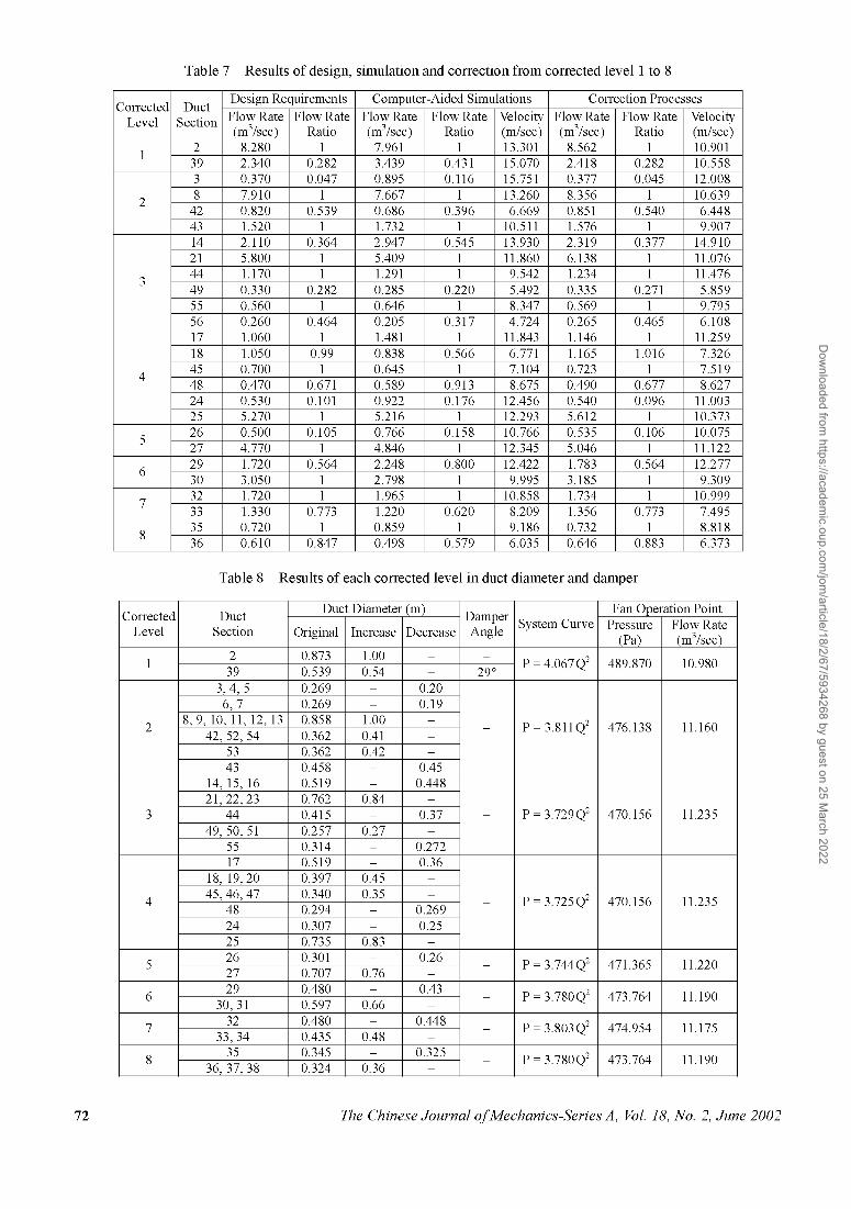
Table 7 Results of design, simulation and correction from corrected level 1 to 8

CorrectedLevel

1Is

)

3

4

5

6

7

8

DuctSection

23938

42431421444955561718454824252627293032333536

Design RequirementsFlow Rate(m3/sec)

8.2802.3400.3707.9100.8201.5202.1105.8001.1700.3300.5600.2601.0601.0500.7000.4700.5305.2700.5004.7701.7203.0501.7201.3300.7200.610

Flow RateRatio

10.2820.047

10.539

10.364

11

0.2821

0.4641

0.991

0.6710.101

10.105

10.564

11

0.7731

0.847

Computer-Aided SimulationsFlow Rate(m3/sec)

7.9613.4390.8957.6670.6861.7322.9475.4091.2910.2850.6460.2051.4810.8380.6450.5890.9225.2160.7664.8462.2482.7981.9651.2200.8590.498

Flow RateRatio

10.4310.116

10.396

10.545

11

0.2201

0.3171

0.5661

0.9130.176

10.158

10.800

11

0.6201

0.579

Velocity(m/sec)13.30115.07015.75113.2606.669

10.51113.93011.8609.5425.4928.3474.724

11.8436.7717.1048.675

12.45612.29310.76612.34512.4229.995

10.8588.2099.1866.035

Correction ProcessesFlow Rate(m3/sec)

8.5622.4180.3778.3560.8511.5762.3196.1381.2340.3350.5690.2651.1461.1650.7230.4900.5405.6120.5355.0461.7833.1851.7341.3560.7320.646

Flow RateRatio

10.2820.045

10.540

10.377

11

0.2711

0.4651

1.0161

0.6770.096

10.106

10.564

11

0.7731

0.883

Velocity(m/sec)10.90110.55812.00810.6396.4489.907

14.91011.07611.4765.8599.7956.108

11.2597.3267.5198.627

11.00310.37310.07511.12212.2779.309

10.9997.4958.8186.373

Table 8 Results of each corrected level in duct diameter and damper

CorrectedLevel

1

Is)

3

4

5

6

7

8

DuctSection

239

3,4,56,7

8,9,10,11,12,1342, 52, 54

5343

14, 15, 1621,22,23

4449, 50, 51

5517

18,19,2045, 46, 47

482425262729

30,3132

33,3435

36, 37, 38

Duct Diameter (m)

Original

0.8730.5390.2690.2690.8580.3620.3620.4580.5190.7620.4150.2570.3140.5190.3970.3400.2940.3070.7350.3010.7070.4800.5970.4800.4350.3450.324

Increase

1.000.54

--

1.000.410.42

--

0.84-

0.27--

0.450.35

--

0.83-

0.76-

0.66-

0.48-

0.36

Decrease

--

0.200.19

---

0.450.448

-0.37

-0.2720.36

--

0.2690.25

-0.26

-0.43

-0.448

-0.325

-

DamperAngle

-29°

-

-

System Curve

P=4.067Q2

P=3.811Q2

P = 3.729 Q2

P = 3.725 Q2

p = 3.744Q2

P=3.780Q2

P=3.803Q2

P=3.780Q2

Fan Operation PointPressure

(Pa)

489.870

476.138

470.156

470.156

471.365

473.764

474.954

473.764

Flow Rate(m3/sec)

10.980

11.160

11.235

11.235

11.220

11.190

11.175

11.190


Dow


ic.oup.com/jom


12

13

21

. . .

22

24

26

29

32

35

38

Exhaust Volume

Jf Damper & Angle

(££25)

Fig. 6 System diagram from 3C duct design method

Figure 7 shows the correlation of average volumeflow rate error between design values and correctionresults at each corrected level. Level 0 represents theresults from initial simulation. Corrected levels 1 to 8indicate correction results through computer-aidedsimulation at each correction process. Each levelcharacterizes the feedback correction times in 3C ductdesign method. As the feedback correction isperforming, the error is effectively reduced. Table 9shows that the results of volume flow rate predictedfrom 3C duct design method is very close to thoseobtained from design requirements. The volume flowrate in initial computer simulation method (level 0), ascompared with that at the original design requirements,has an average error around 42.68%. The volume flowrate predicted from the 3C design method (level 8) hasan average error around 5.405%. It should be notedthat the discrepancy in volume flow rate error for 3Cduct design method is primarily because of systemsafety concerns in the design procedure. That is, a fanprovide volume flow rate greater than the requiredvolume flow rate to meet the demand of allowance ofsafety.

Table 10 shows the results of total surface area, fantotal pressure and volume flow rate at each level'scalculation. The designed duct total surface areadiameter represents a system's initial cost. The totalduct surface area is increasing from level 0 to correctedlevel 8. However, the change in surface area is verysmall. In other words, the adjustment made during

design corrections had a very small impact on the initialcost of entire system. Thus, 3C design method canengage in refined corrections of the original design andachieve the volume flow rate without significantlyaltering the system itself. Besides, the values of fantotal pressure and volume flow rate represent the energycost of system operation. As shown in Table 10, thechange of system volume flow rate is very limited. Itshould be noted that the fan total pressure increasesaround 3%. The reason for the rise in fan totalpressure is due to the absence of a pressure-balancingdevice in initial design process. Dampers are addedduring design corrections, which increase the resistanceand raise the fan total pressure as the number ofcorrections increases. The cost of entire system can beestimated based on construction cost and operating cost.From the above discussion 3C duct design methodrepresents a very precise design method for designing aduct system.

50

45

r 40

& 35

I* 30 -oE 25

= 20o

a . 1 5

2£ 10<

5

0

Fig. 7

-

I I I I i!II h3 4 5

Corrected Levels

Average volume flow rate error at eachcorrected level

Table 9 Comparison of design requirement, initialcomputer-aided simulation and 3C ductdesign method in volume flow rate

DuctSection

717202426293235384748515556

DesignRequirement

Flow Rate(m3/sec)

0.3701.0601.0500.5300.5001.7201.7200.7200.6100.7000.4700.3300.5600.260

InitialComputer-Aided

Simulation (Level 0)Flow Rate (m3/sec)

0.8321.6040.9090.6920.5341.5121.1610.4550.2621.0540.9590.4480.7420.236

3C Duct DesignMethod

Flow Rate(m3/sec)

0.3761.1691.1880.5640.5601.8251.7270.7320.6460.7250.4920.3430.5760.268


Dow


ic.oup.com/jom


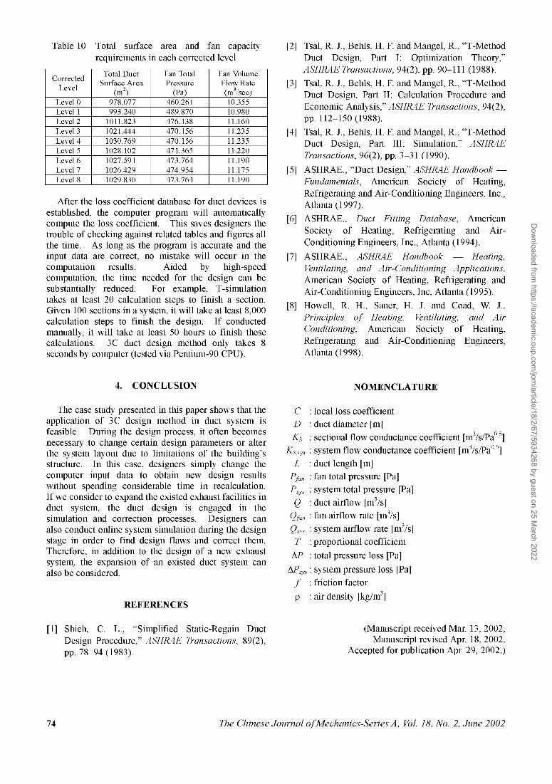
Table 10 Total surface area and fan capacityrequirements in each corrected level

CorrectedLevel

Level 0Level 1Level 2Level 3Level 4Level 5Level 6Level 7Level 8

Total DuctSurface Area

(m2)978.077993.240

1011.8231021.4441030.7691028.1021027.5911026.4291029.830

Fan TotalPressure

(Pa)460.261489.870476.138470.156470.156471.365473.764474.954473.764

Fan VolumeFlow Rate(m3/sec)10.35510.98011.16011.23511.23511.22011.19011.17511.190

After the loss coefficient database for duct devices isestablished, the computer program will automaticallycompute the loss coefficient. This saves designers thetrouble of checking against related tables and figures allthe time. As long as the program is accurate and theinput data are correct, no mistake will occur in thecomputation results. Aided by high-speedcomputation, the time needed for the design can besubstantially reduced. For example, T-simulationtakes at least 20 calculation steps to finish a section.Given 100 sections in a system, it will take at least 8,000calculation steps to finish the design. If conductedmanually, it will take at least 50 hours to finish thesecalculations. 3C duct design method only takes 8seconds by computer (tested via Pentium-90 CPU).

[2] Tsal, R. J., Behls, H. F. and Mangel, R., "T-MethodDuct Design, Part I: Optimization Theory,"ASHRAE Transactions, 94(2), pp. 90-111 (1988).

[3] Tsal, R. J., Behls, H. F. and Mangel, R., "T-MethodDuct Design, Part II: Calculation Procedure andEconomic Analysis," ASHRAE Transactions, 94(2),pp. 112-150(1988).

[4] Tsal, R. J., Behls, H. F. and Mangel, R., "T-MethodDuct Design, Part III: Simulation," ASHRAETransactions, 96(2), pp. 3-31 (1990).

[5] ASHRAE., "Duct Design," ASHRAE Handbook —Fundamentals, American Society of Heating,Refrigerating and Air-Conditioning Engineers, Inc.,Atlanta (1997).

[6] ASHRAE., Duct Fitting Database, AmericanSociety of Heating, Refrigerating and Air-Conditioning Engineers, Inc., Atlanta (1994).

[7] ASHRAE., ASHRAE Handbook — Heating,Ventilating, and Air-Conditioning Applications,American Society of Heating, Refrigerating andAir-Conditioning Engineers, Inc, Atlanta (1995).

[8] Howell, R. H., Sauer, H. J. and Coad, W. J.,Principles of Heating, Ventilating, and AirConditioning, American Society of Heating,Refrigerating and Air-Conditioning Engineers,Atlanta (1998).

4. CONCLUSION NOMENCLATURE

The case study presented in this paper shows that theapplication of 3C design method in duct system isfeasible. During the design process, it often becomesnecessary to change certain design parameters or alterthe system layout due to limitations of the building'sstructure. In this case, designers simply change thecomputer input data to obtain new design resultswithout spending considerable time in recalculation.If we consider to expand the existed exhaust facilities induct system, the duct design is engaged in thesimulation and correction processes. Designers canalso conduct online system simulation during the designstage in order to find design flaws and correct them.Therefore, in addition to the design of a new exhaustsystem, the expansion of an existed duct system canalso be considered.

REFERENCES

CD

KS

KS,sys

L

Pfan

Psys

Q

Qfan

Qsys

T

AP

APsys

fP

local loss coefficientduct diameter [m]sectional flow conductance coefficient [m3/s/Pa°5]system flow conductance coefficient [m3/s/Pa°5]duct length [m]fan total pressure [Pa]system total pressure [Pa]duct airflow [m3/s]fan airflow rate [m3/s]system airflow rate [m3/s]proportional coefficient

total pressure loss [Pa]

system pressure loss [Pa]friction factor

air density [kg/m3]

[1] Shieh, C. L., "Simplified Static-Regain DuctDesign Procedure," ASHRAE Transactions, 89(2),pp. 78-94 (1983).

(Manuscript received Mar. 13, 2002,Manuscript revised Apr. 18, 2002,

Accepted for publication Apr. 29, 2002.)


Dow


ic.oup.com/jom


3c duct design method

Documents