1

3.3 THE OPTIMIZATION BETWEEN TAMDAR DATA ASSIMILATION METHODS AND MODEL CONFIGURATION IN MM5 AND WRF-ARW

Neil Jacobs1*, Peter Childs1, Meredith Croke1, Yubao Liu2, and Xiang-Yu Huang2

1AirDat LLC, Morrisville, NC 27560 2National Center for Atmospheric Research, Boulder, CO 80307

1. INTRODUCTION AND MOTIVATION* Lower and middle-tropospheric observations are disproportionately sparse, both temporally and geographically, when compared to surface observations. The unsubstantial density of observations is likely one of the largest limiting factors in numerical weather prediction. Atmospheric measurements performed by the Tropospheric Airborne Meteorological Data Reporting (TAMDAR) sensor of humidity, pressure, temperature, winds aloft, icing, and turbulence, along with the corresponding location, time, and altitude from built-in GPS are relayed via satellite in real-time to a ground-based network operations center. Since December 2004, the TAMDAR sensors have been operating on a fleet of 63 Saab 340s operated by Mesaba Airlines in the Great Lakes region as a part of the NASA-sponsored Great Lakes Fleet Experiment (GLFE). This fleet was the primary source of data for the study presented in Jacobs et al. (2007, 2008). An example of the flight data density for a typical day in May 2007 is shown in Fig. 1, which is essentially the same density as 2006 (with Mesaba). Equipage of sensors on additional aircraft across the continental US and Alaska is currently underway. An example of the increase in observations and flights can be seen for the same day in May of 2008 (cf. Fig. 1 and Fig. 2).

Fig. 1. Flight routes and observations for 28-29 May 2007

*Corresponding author address: Neil A. Jacobs, AirDat, LLC, 2400 Perimeter Park Dr. Suite 100, Morrisville, NC 27560. Email: njacobs@airdat.com

A study of the impact of the TAMDAR data on mesoscale NWP is conducted using two mesoscale models, which employ various assimilation techniques and the available TAMDAR data. The first study reconducts the sensitivity experiment from Jacobs et al. (2007, 2008) using RAOB observations as verification instead of the North American Regional Reanalysis (NARR). The motivation for changing the verification method is discussed in Jacobs et al. (2008).

Fig. 2. Flight routes and observations for 28-29 May 2008 The study is essentially unchanged from the Jacobs et al. (2008) six parallel 12-h simulations, where the three experimental (control) runs include (withhold) TAMDAR data, are performed, with one of the three pair of experimental and control simulations having 36 σ-levels, while the other two pair of experimental and control simulations have 48 σ-levels. One of the 48-σ-level pairs has a single domain of 10-km grid spacing, while the other two pair have a 36-km outer domain which feeds a 12-km inner domain. The main difference introduced in this study is several additional aircraft from different regions. The additional regions include Alaska, the Pacific Northwest, and most of the CONUS east of the Mississippi. The additional planes (in COUNS) are primarily ERJs, which fly higher than the previous turboprops. With more sophisticated avionics, the ERJs also provide more precise heading information, so it is expected that the wind vectors derived from these airplanes will be more accurate. The objectives of this study are to (i) optimize impacts that TAMDAR data may have on the forecast

2

system by increasing the horizontal distribution of vertical atmospheric profiles during initialization, and (ii) to isolate the effects of various data assimilation techniques at a higher horizontal and vertical resolution with respect to temperature and relative humidity forecast variables.

Table 1. The six different parallel model runs in this study

Fig. 3. The Lambert conformal grid for the outer domain of all the simulations. 2. METHODOLOGY AND MODEL CONFIGURATION There are six parallel model runs in this study (Table 1), which is a continuation of the ongoing analysis described in Jacobs et al. (2008). The AirDat-standard run (AD) features an outer domain of 36-km grid spacing and a two-way nested 12-km inner domain. The AD run has 36 σ-levels and assimilates the TAMDAR data. The AirNot-standard run (AN) has an identical model configuration except AN does not include TAMDAR data. The AirDat-2 (AD2) and AirNot-2 (AN2) runs have an identical nested-domain structure to both the AD and AN runs; however, 12 additional σ-levels have been added in both AD2 and AN2 for a total of 48 levels. As in AD and AN, the only difference between AD2 and AN2 is that AD2 assimilates TAMDAR data, while AN2 does not. The majority of the additional σ-levels for AD2 and AN2 are added in the lowest 3 km, or between the 1000 and 700-hPa pressure-levels. This spacing was chosen to best utilize the observation density provided by the TAMDAR data. The final two parallel simulations are the AirDat-10 (AD10) and the AirNot-10 (AN10). These two runs have only one domain of 10-km grid spacing. This

domain has the same latitude and longitude dimensions as the outer domain of the previously discussed runs. Both the AD10 and AN10 runs have 48 σ-levels, which are identically spaced to those in the AD2 and AN2 runs. Comparisons are drawn between the like-runs (e.g., AD to AN, AD2 to AN2, etc.) to ascertain any TAMDAR-related impacts. Additionally, comparisons are drawn between AD, AD2, and AD10, with the AN runs as controls, to quantify the effects of increased vertical resolution on the utilization of TAMDAR data. Comparisons are also drawn between the AD and AD2 runs to the AD10 run to quantify any change in forecast skill as a function of finer horizontal radial influence during the observation assimilation stage. The final stage compares differences between the current study and the previous year (2007), which had fewer planes with a more limited geography. The study covers the entire month of May 2008. The model cycling and assimilation is left unchanged from the 2007 study, but is covered here again for convenience. The MM5 simulations were initialized at 1800 UTC for all model runs. All simulations were initialized with identical analysis fields provided by the NCAR/AirDat RT-FDDA-MM5. The NCAR/AirDat RT-FDDA system is built around the Fifth Generation of the Penn State/National Center for Atmospheric Research (PSU/NCAR) Mesoscale Model (MM5, Dudhia 1993; Grell et al. 1994). The outer domain of the RT-FDDA-MM5 has a 100 x 97 grid spacing of 36 km, and is centered over the Great Lakes region (Fig. 3). A continuous data ingestion system using Newtonian relaxation is utilized during an analysis period to generate balanced 4-D analyses. This method greatly reduces the time and errors associated with typical model spin-up (Stauffer and Seaman 1994; Cram et al. 2001; and Liu et al. 2002). The NCAR/AirDat RT-FDDA is run on a 3-h cycle with cycle times occurring at 23Z, 2Z, 5Z, 8Z, 11Z, 14Z, 17Z, and 20Z. For this study, the 1-h output from the 1700 UTC RT-FDDA cycle, valid 1800 UTC, were used as first-guess fields. These files include 1 hour of additional 4DDA nudging; however, they do not include TAMDAR data (i.e., AIRNOT cycles). After the first-guess field is generated, it is then passed through a 3DVAR-style technique to assimilate additional observations and construct the analysis from which each MM5 simulation is initialized. All of the additional observations are identical for all runs with the exception of the TAMDAR data, which is only assimilated by the AD runs using this 3DVAR approach.

The MM5 was employed as a means to ascertain optimal combinations and settings for various ingestion, weighting, resolution, and parameterization options. Extensive testing of various parameterizations has been performed to optimize the impact of TAMDAR data (Jacobs and Liu 2006). Those studies suggest that the Kain-Fritsch (KF) cumulus parameterization (CP) is better suited for 20 to 30-km grid spacing, while the Grell CP is better suited for 10-km spacing, and are consistent with findings from Kain and Fritsch (1993). Kain-Fritsch, which generates more convection, may be acceptable if only using the 36-km domain, but when that domain is used as boundary conditions for a finer nested domain

3

such as 12-km, too much convective feedback may occur. Additionally, some CP schemes are better for summer and tropical convection, and some are better for winter mid-latitude convection. Grell tends to handle thunderstorms much better, while KF handles winter frontal systems better (Mahoney and Lackmann 2005).

Based on these findings, as well as the season of the study, the Grell cumulus parameterization was chosen for its handling of convective precipitation at smaller grid scales. The MRF planetary boundary layer scheme, as well as the Mixed-phase (Reisner-1) microphysics were also chosen to be consistent with the analysis field generation methods. All simulations were integrated for 12 hours; however, only the forecast-hour 6 (i.e., 0000 UTC for the 1800 UTC run) was used for verification purposes. This was also done to remain consistent with the previous (2007) study.

For consistency, verification was conducted at the same three locations as the previous study: Minneapolis/St. Paul, MN (KMPX; 44.8489 N, 93.5656 W; Elev: 946'), Detroit/Pontiac, MI (KDTX; 42.6997 N, 83.4717 W; Elev: 1072'), and Green Bay, WI (KGRB; 44.4983 N, 88.1114 W; Elev: 682'). It should be noted that the majority of the ERJs cover a region over, and east, of these hubs, and greater differences from those planes would likely be seen downstream. As in the previous study, the model-generated soundings were compared to RAOB observations. The RH value is obtained from the RAOB temperature and dewpoint using the calculation outlined in Bolton (1980). The forecast bias is simply defined as the 6-hour forecast value (X) minus the observed value (θ). In the case of the 1800 UTC simulations, differences are calculated at 0000 UTC. The forecast RMS error is defined as

!

RMSE(X) =1

nX " X ( )

n=1

n

#2

+ X "$( )2%

& '

(

) *

1

2 , (1)

where n is the number of compared values. Since there is one run a day, for this case it is equal to the number of days. A percent reduction in error is seen as a percentage increase in forecast skill. This percent improvement is defined as

!

%IMP = "# "$

$%100, (2)

where simulation α is compared to simulation β, and appears contextually below as α versus β (Brooks and Doswell 1996). 3. SENSITIVITY TO σ -LEVEL DENSITY AND HORIZONTAL GRID SPACING It should be noted that all of the plots below correspond to the 0000 UTC comparison. The 0000 UTC time historically shows a larger difference because (i) there are more flights between 1400 and 2200 UTC, and (ii) the lower-troposphere is less stable. The figures

presented here are plotted from the average statistics derived from the three locations of verification.

0 0.5 1 1.5 2 2.5

200

400

600

800

1000

Temperature 6-h Forecast RMS Error6-h forecast (from 18 UTC) against 00 UTC RAOBs

ADANAD2AN2AD10AN10

Pre

ssu

re (

hP

a)

Temperature Error (K) Fig. 4. Vertical profile of 6-h temperature RMS error verified against 00 UTC RAOBs for May 2008. Average of the three locations KMPX, KDTX, KGRB. The 6-h temperature forecast error shown in Fig. 4 appears to be greater in magnitude above 300 hPa; however, it is assumed to be unrelated to the TAMDAR data and grid variations since similar trends are seen for all simulations. Despite this increase, error above 400 hPa is about 0.2-0.3 K less than the previous year. Divergence between the simulations begins to occur around 200 hPa. Between 400 and 800 hPa, the error in the runs diverge further, but in general, the error magnitude does not change. The AN/AN2 runs have an average error of around 1.35 K, while the AD and AD2 runs were 1.1 and 1.2 K, respectively -- a reduction across the board including the controls. Below 500 hPa, the AN10/AD10 runs were nearly identical in error to the 2006/07 study; however, between 500 and 200 hPa, the AD10 run averaged approximately 0.3 K less error than the control (AN10). It is evident from these differences that a finer outer grid during the data assimilation phase improves the forecast skill. Below 900 hPa, the error increases at a linear rate unlike what was observed in the previous study.

The method for quantifying forecast skill is given by (2). The improvement as a function of TAMDAR data for temperature is assumed to be the difference in corresponding like-runs in Fig. 4. Minor positive impact is seen for the AD run over the AN run, while the largest improvement noted is between AD2 and AN2. This is different than the previous study, where the largest differences were seen between AD10/AN10. This still supports the hypothesis that vertical resolution plays a role in forecast skill with respect to TAMDAR data assimilation. The differences between the years may be showing that the additional TAMDAR observations (in 2008) are helping improve the skill of the non-10 runs.

4

A vertical profile of the 6-h relative humidity forecast error (%), averaged for the entire month of May 2008, is shown in Fig. 5. All simulations follow a similar trend above 300 hPa. Between 300 and 400 hPa, significant divergences between the two 10-km simulations, as well as the other AD runs appear. The error in both AD10 and AN10 ranges from 15 to 18% above 500 hPa, and improves to as low as 10% near 800 hPa for AD10. The decrease in error seen around the 700 hPa level for the TAMDAR-excluded runs, which was also noted in the previous study, was somewhat expected, as that is a mandatory level, and typically has a large amount of observations. The substantial decrease in error seen in the 2007 study around the 900 hPa level was not apparent in 2008, and since it occurred in all of the runs, it was assumed to be a climatological event unrelated to TAMDAR.

0 5 10 15 20 25

200

400

600

800

1000

Relative Humidity 6-h Forecast RMS Error6-h forecast (from 18 UTC) against 00 UTC RAOBs

ADANAD2AN2AD10AN10

RH Error (%)

Pre

ssu

re (

hP

a)

Fig. 5. Vertical profile of 6-h relative humidity RMS error verified against 00 UTC RAOBs for May 2008. Average of the three locations KMPX, KDTX, KGRB.

The most notable improvement as a function of TAMDAR data appears to be linked to the utilization of RH observations in the AD10 simulation. However, between 400 and 600 hPa, as well as between 750 and 850 hPa, a reduction in error (> 2%) is seen between all of the TAMDAR-included runs and their respective controls. The vertical profile of the 6-h wind forecast error (m s-1) is shown in Fig. 6. An increase in the wind error is seen near the top of the profile. Since all of the simulations align while showing identical trends in this region, it is assumed that this bias is either MM5 code-related or a function of the boundary conditions. This feature was also present in the 2007 study; however, the error here appears to be greater above 200 hPa.

The important focus of the study deals with the differences between the runs, more than the error magnitude, within the lower and middle troposphere. The AD10 simulation clearly outperforms the other runs

throughout the vertical profile, albeit to a lesser degree than the previous year, which is attributed to the increase in skill of both the AD and AD2. The error from 1000 to 400 hPa is steady around 4 m s-1. The addition of TAMDAR data decreased the error by about 0.2 m s-1

between 950 and 800 hPa. Elsewhere, improvements of approximately 0.1 - 0.2 m s-1 are seen for most of the lower and middle troposphere.

2 2.5 3 3.5 4 4.5 5 5.5 6

200

400

600

800

1000

<U, V> Wind 6-h Forecast RMS Error6-h forecast (from 18 UTC) against 00 UTC RAOBs

ADANAD2AN2AD10AN10

Pre

ssu

re (

hP

a)

Wind Error (m s-1) Fig. 6. Vertical profile of 6-h wind RMS error verified against 00 UTC RAOBs for May 2008. Average of the three locations KMPX, KDTX, KGRB. 4. UPDATE ON WRF-ARW TESTING

During the fall of 2008, AirDat added version 3.01 of the WRF-ARW to the fleet of models to test parameterizations and assimilation methods. Several updates to the WRFDA system have been implemented. These include a revised First Guess at Appropriate Time (FGAT) package, which allows for a more accurate calculation of innovation vectors and a more optimal use of observations when their valid time differs from that of the analysis, an observation ingest interface and quality control module, and a TAMDAR observation forward, tangent linear and adjoint operator, which is discussed in Childs et al. (2009).

Results of the WRFDA are compared against the standard 3DVAR MM5. Initial comparisons were done for the 48-h forecasted 850-hPa fields against the operational GDAS analysis. The WRF runs include a no-DA run (control), a MADIS-only no-TAMDAR run, and a full-MADIS complete-TAMDAR (including non-Mesaba fleets) run. Also included (for comparison) is the older MM5, which has been running at AirDat since 2004.

The comparisons between WRFDA and 3DVAR MM5 suggest that the WRF-ARW has a slight edge outside of the data assimilation; however, this is just for one case, and several months of monitoring need to be completed before this can be considered a trend. It should also be mentioned that the assimilation methods

5

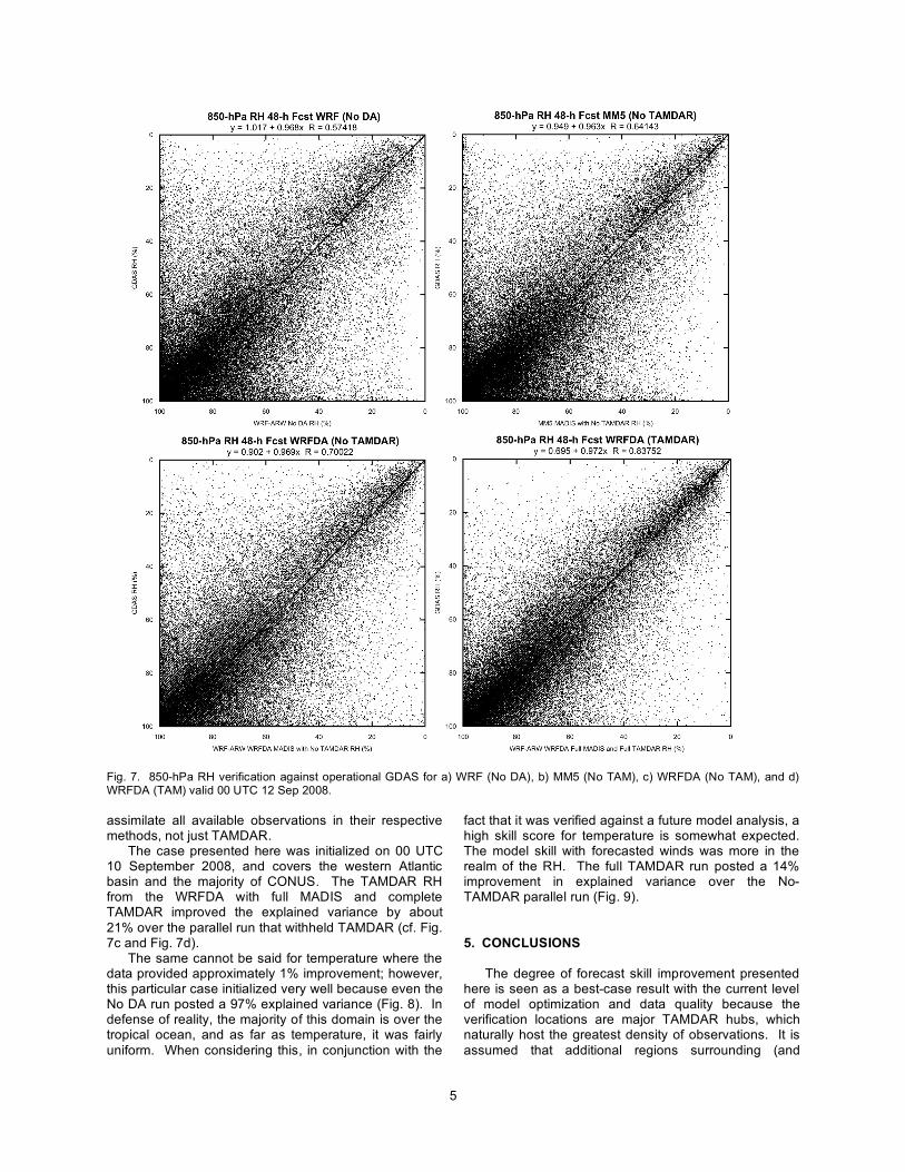
Fig. 7. 850-hPa RH verification against operational GDAS for a) WRF (No DA), b) MM5 (No TAM), c) WRFDA (No TAM), and d) WRFDA (TAM) valid 00 UTC 12 Sep 2008. assimilate all available observations in their respective methods, not just TAMDAR.

The case presented here was initialized on 00 UTC 10 September 2008, and covers the western Atlantic basin and the majority of CONUS. The TAMDAR RH from the WRFDA with full MADIS and complete TAMDAR improved the explained variance by about 21% over the parallel run that withheld TAMDAR (cf. Fig. 7c and Fig. 7d).

The same cannot be said for temperature where the data provided approximately 1% improvement; however, this particular case initialized very well because even the No DA run posted a 97% explained variance (Fig. 8). In defense of reality, the majority of this domain is over the tropical ocean, and as far as temperature, it was fairly uniform. When considering this, in conjunction with the

fact that it was verified against a future model analysis, a high skill score for temperature is somewhat expected. The model skill with forecasted winds was more in the realm of the RH. The full TAMDAR run posted a 14% improvement in explained variance over the No-TAMDAR parallel run (Fig. 9). 5. CONCLUSIONS

The degree of forecast skill improvement presented here is seen as a best-case result with the current level of model optimization and data quality because the verification locations are major TAMDAR hubs, which naturally host the greatest density of observations. It is assumed that additional regions surrounding (and

6

downstream) of future fleet hubs will likely realize similar improvements.

Fig. 8. 850-hPa T verification against operational GDAS for WRF (No DA), MM5 (No TAM), WRFDA (No TAM), and WRFDA (TAM) valid 00 UTC 12 Sep 2008.

Fig. 9. 850-hPa wind vector magnitude verification against operational GDAS for WRF (No DA), MM5 (No TAM), WRFDA (No TAM), and WRFDA (TAM) valid 00 UTC 12 Sep 2008. Results suggest that the addition of TAMDAR data improves all three experimental simulations for key model variables, albeit to various degrees. In general, increasing the number of σ-levels from 36 to 48 results in better utilization of the higher resolution TAMDAR data. The most notable improvements, when increasing the number of model σ-levels, were found to occur in the

vicinity of 850 hPa. This peak is likely a result of the balance between the increase in TAMDAR observations and the increase in expected model error (i.e., seen in the control runs) when approaching the surface layer from the middle-troposphere. This was expected, and has commonly been the case when dealing with TAMDAR data regardless of model type or assimilation method. Changing the outer domain grid spacing from 36 km to 10 km reduces the bias and error for both the experimental (AD10) and the control (AN10); however, the magnitude of reduction is greater in AD10. This is likely because all of the non-TAMDAR observations assimilated into the first-guess fields of both runs improved the respective analysis fields. The additional reduction in error magnitude seen in AD10 is attributed to the TAMDAR data (the only difference between AD10 and AN10).

This study, when compared to the previous (2007) study, showed a much greater improvement in the AD2 run, while not showing gains of similar magnitude in AD10. It is hypothesized that the greater geographic distribution, as well as the larger number of sensors reporting in 2008, played a role in improving the AD2 skill. Additionally, many of these additional planes were ERJs, which reach higher altitudes, and this was where AD2 was previously limited. 6. ACKNOWLEDGMENTS

The authors are very grateful for the technical and computer support provided by NCAR. The authors would like to thank Stan Benjamin (NOAA/ERL/FSL) for his comments and suggestions on RAOBs as a better means of verification. Also, the authors are very grateful to Dr. Tom Rosmond for his valued suggestions and insight during this project. We would like to acknowledge the NASA Aeronautics Research Office’s Aviation Safety Program, the FAA Aviation Weather Research Program, and AirDat, LLC for their support in this effort. Additionally, the authors would like to thank The Tropical Prediction Center for the timely availability of observed and model forecast data for Hurricane Ike. 7. REFERENCES Bolton, D., 1980: The Computation of Equivalent Potential Temperature. Mon. Wea. Rev., 108, 1046-1053. Brooks, H. E., and C. A. Doswell, 1996: A Comparison of Measures-Oriented and Distributions-Oriented Approaches to Forecast Verification. Weather and Forecasting, 11, 288-303. Childs, P., N. Jacobs, M. Croke, Y. Liu, and X. Y. Huang, 2009: TAMDAR-Related Impacts on the AirDat Operational WRF-ARW as a Function of Data Assimilation Techniques, (IOAS-AOLS), AMS, Phoenix, AZ.

7

Cram, J. M., Y. Liu, S. Low-Nam, R-S. Sheu, L. Carson, C. A. Davis, T. Warner, J. F. Bowers, 2001: An operational mesoscale RT-FDDA analysis and forecasting system. Preprints 18th WAF and 14th NWP Confs., Ft. Lauderdale, AMS, Boston, MA. Dudhia, J., 1993: A nonhydrostatic version of the Penn State / NCAR mesoscale model: Validation tests and simulation of an Atlantic cyclone and cold front. Mon. Wea. Rev., 121,1493-1513. Grell, G. A., 1993: Prognostic evaluation of assumptions used by cumulus parameterizations. Mon. Wea. Rev., 121, 764-787. Grell, G. A., J. Dudhia, and D. R. Stauffer, 1994: A description of the Fifth-Generation Penn State/NCAR Mesoscale Model (MM5). NCAR Tech. Note NCAR/TN-398+STR,122 pp. Jacobs, N. A., and Y. Liu, 2006: A Comprehensive Quantitative Precipitation Forecast Statistical Verification Study, Documentation and Tech. Note AirDat, LLC, 25 pp. Jacobs, N. A, Y. Liu, and C.-M. Druse, 2007: The effects of vertical resolution on the optimization of TAMDAR data in short-range mesoscale forecasts, AMS Annual Meeting, 11th Symp. IOAS-AOLS.

Jacobs, N., P. Childs, M. Croke, and Y. Liu, 2008: The Effects of Horizontal Grid Spacing and Vertical Resolution on TAMDAR Data assimilation in Short-Range Mesoscale Forecasts, AMS Annual Meeting, 12th Symposium on Integrated Observing and Assimilation Systems for the Atmosphere, Oceans, and Land Surface (IOAS-AOLS). Kain, J. S., and J. M. Fritsch, 1993: Convective parameterization for mesoscale models: The Kain-Fritsch scheme. The representation of cumulus convection in numerical models, K. A. Emanuel and D. J. Raymond, Eds., Amer. Meteor. Soc., 246 pp. Liu, Y., S. Low-Nam, R. Sheu, L. Carson, C. Davis, T. Warner, S. Swerdlin, J. Bowers, M. Xu, H-M Hsu, and D. Rife, 2002: Performance and Enhancement of the NCAR/ATEC mesoscale FDDA and forecast system. 15th Conference on Numerical Weather Prediction, 12-16 August, 2002, San Antonio, Taxes, 399-402. Mahoney, K.M., and G.M. Lackmann, 2006: The sensitivity of numerical forecasts to convective parameterization: A case study of the 17 February 2004 east coast cyclone. Wea. Forecasting, 21, 465–488. Stauffer, D. R., and N. L. Seaman, 1994: Multiscale four-dimensional data assimilation. J. Appl. Meteor., 33, 416-434.