Earth Planets Space, 51, 1135–1143, 1999

2D inversion of 3D magnetotelluric data: The Kayabe dataset

Xavier Garcia1, Juanjo Ledo1,2, and Pilar Queralt2

1Geological Survey of Canada, 615 Booth Street, Ottawa, Ontario, K1A 0E9, Canada2Departament de Geodinamica i Geofısica, Universitat de Barcelona, Spain

(Received November 9, 1998; Revised May 13, 1999; Accepted May 17, 1999)

In the last two Magnetotelluric Data Interpretation Workshops (MT-DIW) the participants were asked to modelthe Kayabe magnetotelluric dataset, a dense (100 m) grid of thirteen lines, with thirteen stations in each line. Bahr’sphase-sensitive skew and the Groom and Bailey decomposition were used to select those lines for which the datacould be considered two-dimensional. For these lines we used a 2D inversion algorithm to obtain a series of resistivitymodels for the earth. Finally, we constructed a 3D model using the 2D models and critically examined the validityand practicality of this approach based on 3D model study. We found that in the Kayabe dataset case the commonpractice of using 2D models to depict 3D models, can only be used to create a starting model for 3D interpretation.The sequential 2D models as a representation of a 3D body is unacceptable in terms of fit to the observed data. Wequestion the validity of some of the conductivity structures in the 2D models, as they can be mere artifacts createdby the algorithm to match 3D effects.

1. IntroductionThe main objective of MT-DIW3 and MT-DIW4 was to

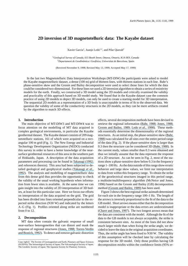
focus attention on the modelling of MT data acquired incomplex geological environments, in particular the Kayabegeothermal dataset. The Kayabe dataset consists of 209 mag-netotelluric stations, 161 of which were acquired on a rect-angular 100 m grid (Fig. 1). The New Energy and IndustrialTechnology Development Organization (NEDO) conductedthis survey in order to have a better knowledge of the near-surface geothermal resources of this area in the southern partof Hokkaido, Japan. A description of the data acquisitionparameters and processing can be found in Takasugi (1992;and references therein). This area had been subjected to de-tailed geological and geophysical studies (Takasugi et al.,1992). The analysis and modelling of magnetotelluric datafrom this dense grid thus provides the opportunity to checkthe validity of the usual working hypothesis when informa-tion from fewer sites is available. At the same time we cangain insight into the validity of 2D interpretation of 3D bod-ies, at least for this particular case. Here we focus our effortson interpretation of the data acquired on the grid. The gridhas been divided into lines oriented perpendicular to the ex-pected strike direction (N30 W) and indicated by the lettersA–G (Fig. 1). Profiles oriented along strike are numberedfrom 0 to 12.

2. DecompositionMT data often contain the galvanic response of small

near-surface heterogeneities that can distort and mask theresponse of regional structures (Jones, 1988; Torres-Verdinand Bostick, 1992). To detect and remove galvanic distortion

Copy right c© The Society of Geomagnetism and Earth, Planetary and Space Sciences(SGEPSS); The Seismological Society of Japan; The Volcanological Society of Japan;The Geodetic Society of Japan; The Japanese Society for Planetary Sciences.

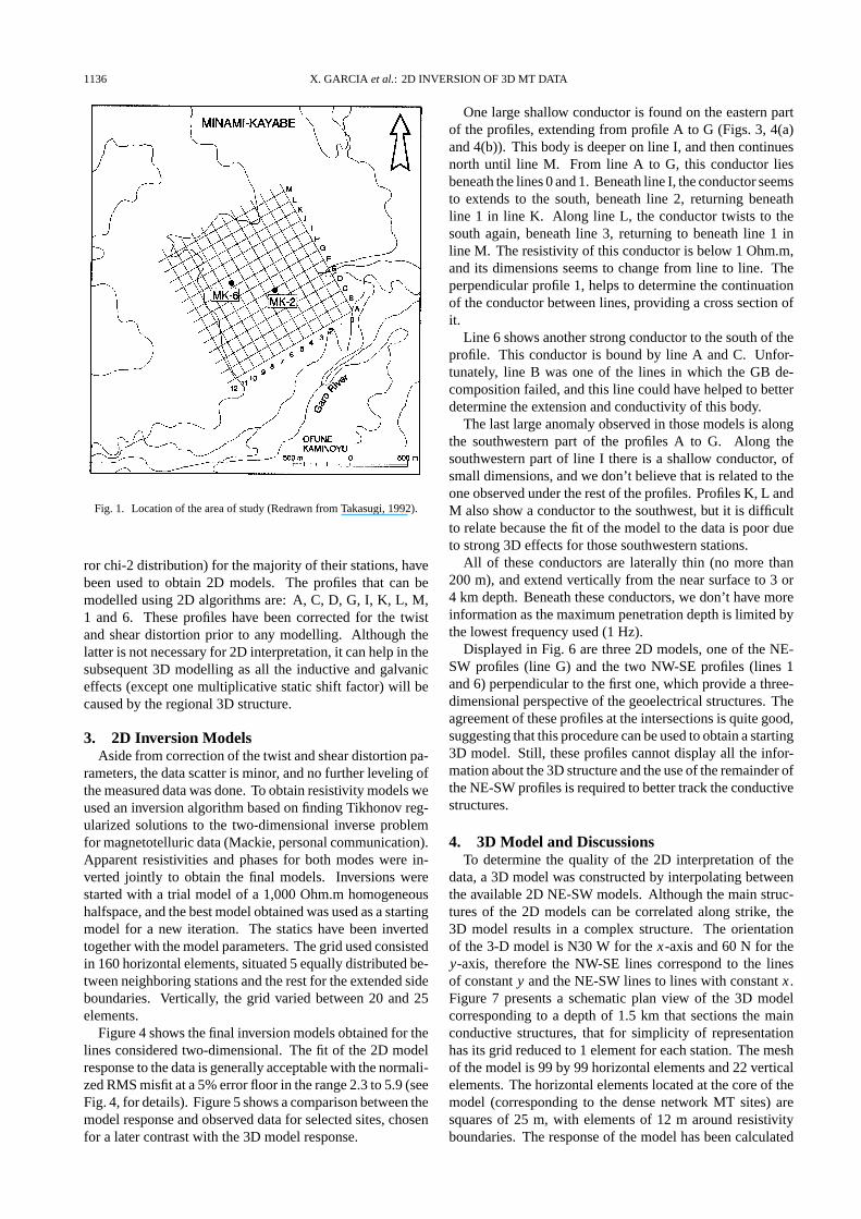
effects, several decomposition methods have been devised toretrieve the regional information (Bahr, 1988; Jones, 1988;Groom and Bailey, 1989; Ledo et al., 1998). These meth-ods essentially determine the dimensionality of the regionalstructures. As an initial step, the phase-sensitive skew (Bahr,1988) was calculated for all sites over the entire period rangeof the data (Fig. 2). If the phase-sensitive skew is larger than0.3 then the structure can be considered 3D (Bahr, 1988). Inthe current study, values smaller than 0.3 were obtained andthus we initially assume that the data represent the responseof a 2D structure. As can be seen in Fig. 2, most of the sta-tions show a phase-sensitive skew below 0.3 in the frequencyrange 1–100 Hz. As the data outside of this range show erraticbehavior and large skew values, we limit our interpretationto data from within this frequency range. To obtain the strikeof the geoelectrical structures imaged in this period range,a multisite/multifrequency algorithm (McNeice and Jones,1996) based on the Groom and Bailey (GB) decompositionmethod (Groom and Bailey, 1989) has been used.

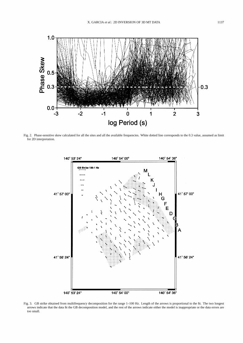
Figure 3 shows the best regional strike azimuth determinedfor each site in the frequency range 100–1 Hz. The length ofthe arrows is inversely proportional to the fit of the data to theGB model. Short arrows means either that the decompositionmodel is inappropriate or the data errors are underestimated(Chave and Jones, 1997). The two longest arrows mean thatthe data are consistent with the model. Although the fit of thedata to the GB models is not always acceptable, the strike isconsistent between sites. As most of the lines did not showmuch larger misfit than when fixing the strike angle, we de-cided to leave the data in the original acquisition coordinates.Thus, the strike angle has been fixed to N30 W. The validityof this assumption will be checked later by calculating theresponse for the 3D model. Only those profiles having GBdecomposition misfits within the confidence limits (95% er-

1135

1136 X. GARCIA et al.: 2D INVERSION OF 3D MT DATA

Fig. 1. Location of the area of study (Redrawn from Takasugi, 1992).

ror chi-2 distribution) for the majority of their stations, havebeen used to obtain 2D models. The profiles that can bemodelled using 2D algorithms are: A, C, D, G, I, K, L, M,1 and 6. These profiles have been corrected for the twistand shear distortion prior to any modelling. Although thelatter is not necessary for 2D interpretation, it can help in thesubsequent 3D modelling as all the inductive and galvaniceffects (except one multiplicative static shift factor) will becaused by the regional 3D structure.

3. 2D Inversion ModelsAside from correction of the twist and shear distortion pa-

rameters, the data scatter is minor, and no further leveling ofthe measured data was done. To obtain resistivity models weused an inversion algorithm based on finding Tikhonov reg-ularized solutions to the two-dimensional inverse problemfor magnetotelluric data (Mackie, personal communication).Apparent resistivities and phases for both modes were in-verted jointly to obtain the final models. Inversions werestarted with a trial model of a 1,000 Ohm.m homogeneoushalfspace, and the best model obtained was used as a startingmodel for a new iteration. The statics have been invertedtogether with the model parameters. The grid used consistedin 160 horizontal elements, situated 5 equally distributed be-tween neighboring stations and the rest for the extended sideboundaries. Vertically, the grid varied between 20 and 25elements.

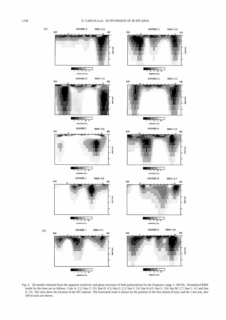
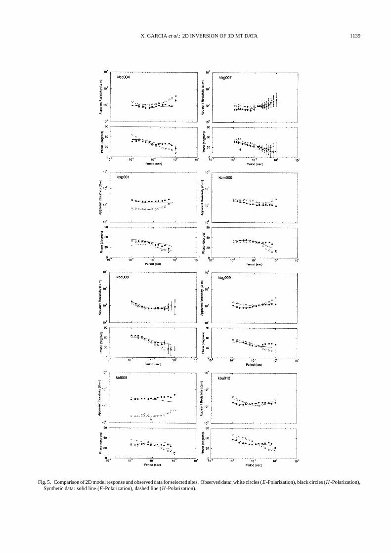
Figure 4 shows the final inversion models obtained for thelines considered two-dimensional. The fit of the 2D modelresponse to the data is generally acceptable with the normali-zed RMS misfit at a 5% error floor in the range 2.3 to 5.9 (seeFig. 4, for details). Figure 5 shows a comparison between themodel response and observed data for selected sites, chosenfor a later contrast with the 3D model response.

One large shallow conductor is found on the eastern partof the profiles, extending from profile A to G (Figs. 3, 4(a)and 4(b)). This body is deeper on line I, and then continuesnorth until line M. From line A to G, this conductor liesbeneath the lines 0 and 1. Beneath line I, the conductor seemsto extends to the south, beneath line 2, returning beneathline 1 in line K. Along line L, the conductor twists to thesouth again, beneath line 3, returning to beneath line 1 inline M. The resistivity of this conductor is below 1 Ohm.m,and its dimensions seems to change from line to line. Theperpendicular profile 1, helps to determine the continuationof the conductor between lines, providing a cross section ofit.

Line 6 shows another strong conductor to the south of theprofile. This conductor is bound by line A and C. Unfor-tunately, line B was one of the lines in which the GB de-composition failed, and this line could have helped to betterdetermine the extension and conductivity of this body.

The last large anomaly observed in those models is alongthe southwestern part of the profiles A to G. Along thesouthwestern part of line I there is a shallow conductor, ofsmall dimensions, and we don’t believe that is related to theone observed under the rest of the profiles. Profiles K, L andM also show a conductor to the southwest, but it is difficultto relate because the fit of the model to the data is poor dueto strong 3D effects for those southwestern stations.

All of these conductors are laterally thin (no more than200 m), and extend vertically from the near surface to 3 or4 km depth. Beneath these conductors, we don’t have moreinformation as the maximum penetration depth is limited bythe lowest frequency used (1 Hz).

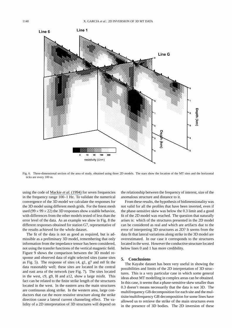
Displayed in Fig. 6 are three 2D models, one of the NE-SW profiles (line G) and the two NW-SE profiles (lines 1and 6) perpendicular to the first one, which provide a three-dimensional perspective of the geoelectrical structures. Theagreement of these profiles at the intersections is quite good,suggesting that this procedure can be used to obtain a starting3D model. Still, these profiles cannot display all the infor-mation about the 3D structure and the use of the remainder ofthe NE-SW profiles is required to better track the conductivestructures.

4. 3D Model and DiscussionsTo determine the quality of the 2D interpretation of the

data, a 3D model was constructed by interpolating betweenthe available 2D NE-SW models. Although the main struc-tures of the 2D models can be correlated along strike, the3D model results in a complex structure. The orientationof the 3-D model is N30 W for the x-axis and 60 N for they-axis, therefore the NW-SE lines correspond to the linesof constant y and the NE-SW lines to lines with constant x .Figure 7 presents a schematic plan view of the 3D modelcorresponding to a depth of 1.5 km that sections the mainconductive structures, that for simplicity of representationhas its grid reduced to 1 element for each station. The meshof the model is 99 by 99 horizontal elements and 22 verticalelements. The horizontal elements located at the core of themodel (corresponding to the dense network MT sites) aresquares of 25 m, with elements of 12 m around resistivityboundaries. The response of the model has been calculated

X. GARCIA et al.: 2D INVERSION OF 3D MT DATA 1137

Fig. 2. Phase-sensitive skew calculated for all the sites and all the available frequencies. White dotted line corresponds to the 0.3 value, assumed as limitfor 2D interpretation.

Fig. 3. GB strike obtained from multifrequency decomposition for the range 1–100 Hz. Length of the arrows is proportional to the fit. The two longestarrows indicate that the data fit the GB decomposition model, and the rest of the arrows indicate either the model is inappropriate or the data errors aretoo small.

1138 X. GARCIA et al.: 2D INVERSION OF 3D MT DATA

(a)

(b)

Fig. 4. 2D models obtained from the apparent resistivity and phase inversion of both polarizations for the frequency range 1–100 Hz. Normalized RMSmisfit for the lines are as follows: Line A: 2.3; line C: 3.9; line D: 4.3; line G: 2.3; line I: 5.9; line K:4.5; line L: 2.6; line M: 2.7; line 1: 4.1 and line6: 2.6. The stars show the location of the MT stations. The horizontal scale is shown by the position of the first station (0 km), and the 1 km tick, also100 m ticks are shown.

X. GARCIA et al.: 2D INVERSION OF 3D MT DATA 1139

Fig. 5. Comparison of 2D model response and observed data for selected sites. Observed data: white circles (E-Polarization), black circles (H -Polarization),Synthetic data: solid line (E-Polarization), dashed line (H -Polarization).

1140 X. GARCIA et al.: 2D INVERSION OF 3D MT DATA

Fig. 6. Three-dimensional section of the area of study, obtained using three 2D models. The stars show the location of the MT sites and the horizontalticks are every 100 m.

using the code of Mackie et al. (1994) for seven frequenciesin the frequency range 100–1 Hz. To validate the numericalconvergence of the 3D model we calculate the responses forthe 3D model using different mesh grids. For the finest meshused (99×99×22) the 3D responses show a stable behavior,with differences from the other models tested of less than theerror level of the data. As an example we show in Fig. 8 thedifferent responses obtained for station G7, representative ofthe results achieved for the whole dataset.

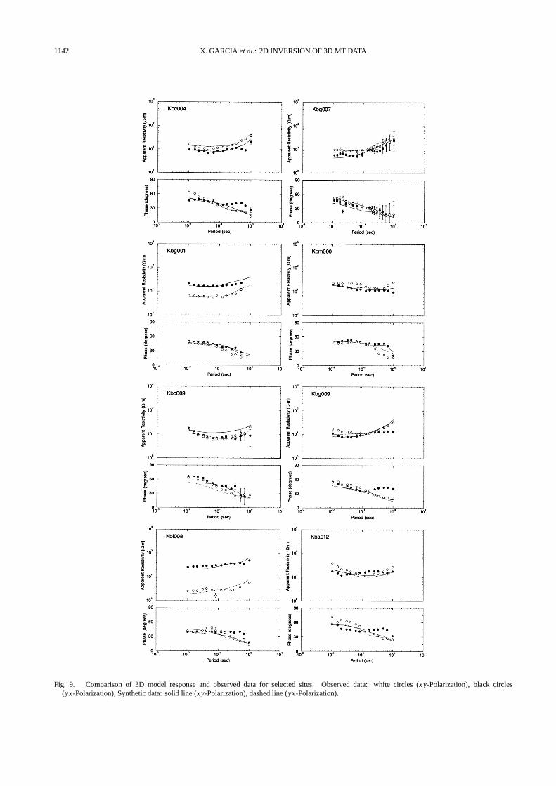
The fit of the data is not as good as required, but is ad-missible as a preliminary 3D model, remembering that onlyinformation from the impedance tensor has been considered,not using the transfer functions of the vertical magnetic field.Figure 9 shows the comparison between the 3D model re-sponse and observed data of eight selected sites (same sitesas Fig. 5). The response of sites c4, g1, g7 and m0 fit thedata reasonably well; these sites are located in the centraland east area of the network (see Fig. 7). The sites locatedin the west, c9, g9, l8 and a12, show a large misfit. Thisfact can be related to the finite strike length of the structureslocated in the west. In the eastern area the main structuresare continuous along strike. In the western area, large con-ductors that cut the more resistive structure along the strikedirection cause a lateral current channeling effect. The va-lidity of a 2D interpretation of 3D structures will depend on

the relationship between the frequency of interest, size of theanomalous structure and distance to it.

From these results, the hypothesis of bidimensionality wasnot valid for all the profiles that have been inverted, even ifthe phase-sensitive skew was below the 0.3 limit and a goodfit of the 2D model was reached. The question that naturallyarises is: which of the structures presented in the 2D modelcan be considered as real and which are artifacts due to theerror of interpreting 3D structures as 2D? It seems from thedata fit that lateral variations along strike in the 3D model areoverestimated. In our case it corresponds to the structureslocated in the west. However the conductive structure locatedbelow lines 0 and 1 has more credibility.

5. ConclusionsThe Kayabe dataset has been very useful in showing the

possibilities and limits of the 2D interpretation of 3D struc-tures. This is a very particular case in which some generalideas about MT modelling in complex areas can be obtained.In this case, it seems that a phase-sensitive skew smaller than0.3 doesn’t means necessarily that the data is not 3D. Themultifrequency GB decomposition for each site and the mul-tisite/multifrequency GB decomposition for some lines haveallowed us to retrieve the strike of the main structures evenin the presence of 3D bodies. The 2D inversion of these

X. GARCIA et al.: 2D INVERSION OF 3D MT DATA 1141

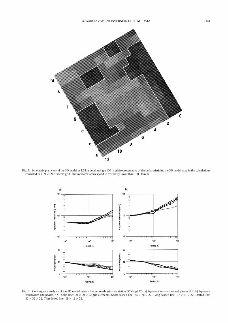
Fig. 7. Schematic plan view of the 3D model at 1.5 km depth using a 100 m grid representative of the bulk resistivity, the 3D model used in the calculationsconsisted in a 99 × 99 elements grid. Outlined areas correspond to resistivity lower than 100 Ohm.m.

Fig. 8. Convergence analysis of the 3D model using different mesh grids for station G7 (kbg007). a) Apparent resistivities and phases XY . b) Apparentresistivities and phases Y X . Solid line: 99 × 99 × 22 grid elements. Short dashed line: 74 × 76 × 22. Long dashed line: 57 × 61 × 22. Dotted line:32 × 32 × 22. Thin dotted line: 19 × 19 × 22.

1142 X. GARCIA et al.: 2D INVERSION OF 3D MT DATA

Fig. 9. Comparison of 3D model response and observed data for selected sites. Observed data: white circles (xy-Polarization), black circles(yx-Polarization), Synthetic data: solid line (xy-Polarization), dashed line (yx-Polarization).

X. GARCIA et al.: 2D INVERSION OF 3D MT DATA 1143

profiles gives us a first approach to the electrical structurewith a good data fit for all the sites along the lines. However,when a 3D model was created using the 2D models, the misfitpresents an important bias and it is not uniformly distributed.The sites located near finite strike structures have larger mis-fits. This result must be related to lateral current channelingeffects, due to the lateral finite extension of the structures.The current channeling introduces false structures in the 2Dmodels. Although not all the available data have been used,the 3D model obtained from the 2D data inversion will be auseful starting model.

Acknowledgments. NEDO kindly allows us the use of this data.The authors would like to thank Alan G. Jones, David Boerner andDon White for the comments and suggestions. Two anonymousreviewers and John Weaver are also acknowledged. XG gratefullyacknowledges the MT-DIW4 organization for the financial supportto attend the workshop held in Sinaia. The attendance of PQ atthe MT-DIW4 was supported by DGICYT of Spain, project PB95-0269. The attendance of JL was supported by a grant from theSpanish Ministry of Education. GSC contribution 1999048.

ReferencesBahr, K., Interpretation of the magnetotelluric impedance tensor: regional

induction and local telluric distortion, J. Geophys., 62, 119–127, 1988.

Chave, A. and A. G. Jones, Electric and magnetic field galvanic distortiondecomposition of BC87 data, J. Geomag. Geoelectr., 49, 767–789, 1997.

Groom, R. W. and R. C. Bailey, Decomposition of magnetotelluric im-pedance tensors in the presence of local three-dimensional galvanic dis-tortions, J. Geophys. Res., 94, 1913–1925, 1989.

Jones, A. G., Static shift of magnetotelluric and its removal in a sedimentaryenvironment, Geophysics, 43, 1157–1166, 1988.

Ledo, J. J., P. Queralt, and J. Pous, Effects of galvanic distortion on magne-totelluric data over a three-dimensional structures, Geophys. J. Int., 132,295–301, 1998.

Mackie, R. L., J. T. Smith, and T. R. Madden, Three-dimensional electro-magnetic modeling using finite difference equations: the magnetotelluricexample, Radio Sci., 29(4), 923–935, 1994.

McNeice, G. and A. G. Jones, Multisite, multifrequency tensor decomposi-tion of magnetotelluric data, in Society of Exploration Geophysicists 66thAnnual Meeting, Expanded Abstracts, pp. 281–284, 1996.

Takasugi, S., Analyses of magnetotelluric fields for a three dimensionalEarth on the basis of the transfer functions, J. Geomag. Geoelectr., 44,325–344, 1992.

Takasugi, S., K. Tanaka, N. Kawakami, and S. Muramatsu, High spa-tial resolution of the resistivity structure revealed by a dense networkMT measurements—A case study in the Minabikayabe area, Hokkaido,Japan, J. Geomag. Geoelectr., 44, 289–308, 1992.

Torres-Verdin, C. and F. X. Bostick, Implication of the Born approxima-tion for the magnetotelluric problem in three-dimensional environments,Geophysics, 57, 587–602, 1992.

X. Garcia (e-mail: garcia@cg.nrcan.gc.ca), J. Ledo, and P. Queralt