28590.pdf - durham research online
TRANSCRIPT
Durham Research Online
Deposited in DRO:
02 July 2019
Version of attached �le:
Published Version
Peer-review status of attached �le:
Peer-reviewed
Citation for published item:
Berg�e, J. and Massey, R. and Baghi, Q. and Touboul, P. (2019) 'Exponential shapelets : basis functions fordata analysis of isolated features.', Monthly notices of the Royal Astronomical Society., 486 (1). pp. 544-559.
Further information on publisher's website:
https://doi.org/10.1093/mnras/stz787
Publisher's copyright statement:
c© 2019 The Author(s). Published by Oxford University Press on behalf of the Royal Astronomical Society.
Use policy
The full-text may be used and/or reproduced, and given to third parties in any format or medium, without prior permission or charge, forpersonal research or study, educational, or not-for-pro�t purposes provided that:
• a full bibliographic reference is made to the original source
• a link is made to the metadata record in DRO
• the full-text is not changed in any way
The full-text must not be sold in any format or medium without the formal permission of the copyright holders.
Please consult the full DRO policy for further details.
Durham University Library, Stockton Road, Durham DH1 3LY, United KingdomTel : +44 (0)191 334 3042 | Fax : +44 (0)191 334 2971
https://dro.dur.ac.uk
MNRAS 486, 544–559 (2019) doi:10.1093/mnras/stz787Advance Access publication 2019 March 16
Exponential shapelets: basis functions for data analysis of isolated features
Joel Berge,1‹ Richard Massey ,2 Quentin Baghi3 and Pierre Touboul41DPHY, ONERA, Universite Paris Saclay, F-92322 Chatillon, France2Centre for Extragalactic Astronomy, Department of Physics, Durham University, Durham DH1 3LE, UK3NASA Goddard Space Flight Center, 8800 Greenbelt Rd, Greenbelt, MD 20771, USA4DSG, ONERA, Universite Paris Saclay, Chemin de la Huniere, F-91123 Palaiseau Cedex, France
Accepted 2019 March 8. Received 2019 February 20; in original form 2018 December 19
ABSTRACTWe introduce one- and two-dimensional ‘exponential shapelets’: orthonormal basis functionsthat efficiently model isolated features in data. They are built from eigenfunctions of thequantum mechanical hydrogen atom, and inherit mathematics with elegant properties underFourier transform, and hence (de)convolution. For a wide variety of data, exponential shapeletscompress information better than Gauss–Hermite/Gauss–Laguerre (‘shapelet’) decomposition,and generalize previous attempts that were limited to 1D or circularly symmetric basisfunctions. We discuss example applications in astronomy, fundamental physics, and spacegeodesy.
Key words: methods: data analysis.
1 IN T RO D U C T I O N
A frequent task in data analysis is to categorize and quantifythe shapes of localized objects – such as transient events in a(one-dimensional) time-series, or regions of interest in a (two-dimensional) image. It is such a universal challenge that methodsdeveloped for one field frequently turn out to be useful in others.For example, astrophysicists measure the shapes of distant galaxiesby decomposing them into orthogonal basis functions, such asCHEFs (Jimenez-Teja & Benıtez 2012) or (Gaussian) shapelets(Bernstein & Jarvis 2002; Refregier 2003; Refregier & Bacon 2003;Massey & Refregier 2005). Shapelets have been used to analysedata in other branches of astrophysics, modelling extrasolar planets(Hoekstra et al. 2005; Amara & Quanz 2012), the distribution ofdark matter (Birrer, Amara & Refregier 2015; Tagore & Jackson2016), or flashes of pulsars (Ellis & Cornish 2015; Lentati et al.2015; Desvignes et al. 2016). They have also been used in medicalimaging (Weissman, Hancewicz & Kaplan 2004; Apostolopouloset al. 2017), pattern recognition in human vision (Sharpee &Victor 2009) or artificial vision (Sabzmeydani & Mori 2007), datacompression (Holbrey 2006), and the manufacture of nanoscale thinfilms (Suderman & Lizotte 2015; Akdeniz, Lizotte & MohieddinAbukhdeir 2018).
Gaussian shapelets are based on eigenfunctions of the quantummechanics harmonic oscillator. In one-dimensional form, they areGauss–Hermite functions, which seem to be well adapted in severaltime-series analyses, especially when transients (whose shape isclose to damped oscillations) must be detected, characterized,and/or corrected for. This is the case for instance in fundamental
� E-mail: [email protected]
physics for MICROSCOPE ‘crackles’ (e.g. Baghi et al. 2015;Berge et al. 2015), space geodesy for GRACE ‘twangs’ (Flury,Bettadpur & Tapley 2008; Peterseim, Jakob & Schlicht 2010;Peterseim et al. 2014), or ‘glitches’ in gravitational wave searcheswith LIGO (Cornish & Littenberg 2015; Powell et al. 2015, 2017;Principe & Pinto 2017 and references therein). In two-dimensionalform, they can be expressed equivalently as either Gauss–Hermite(Cartesian; Refregier 2003) or Gauss–Laguerre (polar; Bernstein &Jarvis 2002; Massey & Refregier 2005) functions. Owing to theirquantum mechanical origin, they have elegant properties (they makea complete set) under Fourier transform, and are hence efficient foroperations involving convolution or deconvolution of two images.
The main limitation of shapelets is that they are perturbationsaround a Gaussian, which is flat near its peak. They inefficientlyparametrize peaky features, including the distant galaxies for whichthey were originally suggested (Melchior et al. 2010). Galaxies havea two-dimensional surface density that decreases approximatelyexponentially with distance from the centre. Capturing the steepgradient near the centre requires a weighted sum of many Gaussianshapelet basis functions, which then overfit noise in the extendedwings. Attempting to overcome this limitation, Ngan et al. (2009)developed ‘Sersiclets’, although they were forced to be circularlysymmetric, and have not seen wider applications.
In this paper, we extend the quantum mechanical frameworkunderpinning Gaussian shapelets, and define 1D and 2D exponentialshapelets based on wavefunctions of the hydrogen atom. Thesefunctions are perturbations around a decreasing exponential, andshould efficiently model any arbitrarily shaped but centrally peakedregions of interest. The perturbations themselves are Laguerrepolynomials.
We introduce 1D exponential shapelets in Section 2, and 2Dexponential shapelets in Section 3. In both cases, we describe their
C© 2019 The Author(s)Published by Oxford University Press on behalf of the Royal Astronomical Society
Dow
nloaded from https://academ
ic.oup.com/m
nras/article-abstract/486/1/544/5382063 by University of D
urham user on 02 July 2019
Exponential shapelets 545
main properties, compare them to Gaussian shapelets, and provideexample uses. We conclude in Section 4.
2 1 D EXPONENTIAL SHAPELETS
2.1 Definition
The 1D hydrogen atom is the solution to the motion of a particle ina 1D Coulomb potential 1/|x|. In this paper, we will neither dwell onits rich history, nor the debates about the finitude of its ground state,and about the existence of even wavefunctions (see Nieto 1979;Palma & Raff 2006; Nu nez-Yepez, Salas-Brito & Solis 2011, 2014and references therein). Instead, we simply exploit the normalized1D hydrogen atom wavefunctions as given by Palma & Raff (2006)to define the 1D exponential shapelet basis functions
�+n (x; β)= (−1)n−1√
n3β
2x
nβL1
n−1
(2x
nβ
)exp
(− x
nβ
)∀x � 0, (1)
for n ≥ 1, where L1n−1 are the generalized Laguerre polynomials
(see e.g. Massey & Refregier 2005). The characteristic scale size β
corresponds to the Bohr radius, and n is the eigenfunction energylevel.
Note that, contrary to normal procedure in quantum physics, werestrict 1D exponential shapelets on positive x, and refrain fromdefining the negative-x part �−
n (x; β) = −�+n (−x; β) (for x < 0).
Hence, we do not follow Palma & Raff (2006) and do not define theeven and odd wavefunctions �+
n (x; β) ± �−n (x; β). Events in time-
series can often be adequately described by their behaviour after acertain moment (in this case, x = 0). Henceforth, we shall thereforedrop the + superscript, to write more simply �n(x; β) ≡ �+
n (x; β).These functions are continuously differentiable, smoothly departingfrom zero at x = 0 and tending back to zero as x → ∞.
Because the basis functions (1) are eigenfunctions of the 1Dhydrogen atom’s Hamiltonian, they form an orthogonal basis ofthe square integrable functions L2([0, ∞[, 〈 ·, ·〉) Hilbert spaceequipped with the inner product 〈f (x), g(x)〉 = ∫ ∞
0 f (x)g∗(x)dx
and an asterisk denotes complex conjugation. They are orthonor-mal, in the sense that
∫ ∞0 �n(x; β)�m(x; β) dx = δnm, where
δnm is the Kronecker symbol, and complete, in the sense that∑∞n=1 �n(x; β)�n(x ′; β) = δ(x − x ′).They thus form a basis on which we can uniquely decompose a
function as
f (x) =∞∑
n=1
fn�n(x; β), (2)
with coefficients fn given by an overlap integral
fn =∫ ∞
0f (x)�n(x; β) dx. (3)
Bessel’s inequality then assures us that for any function f ∈ L2([0,∞[, 〈 ·, ·〉),
∞∑n=1
|fn|2 � ||f ||2, (4)
where ||.|| is the L2 norm, so that the series (2) converges andcoefficients fn must vanish as n increases. The series can thereforebe truncated for suitably localized functions, at some value n ≤nmax.
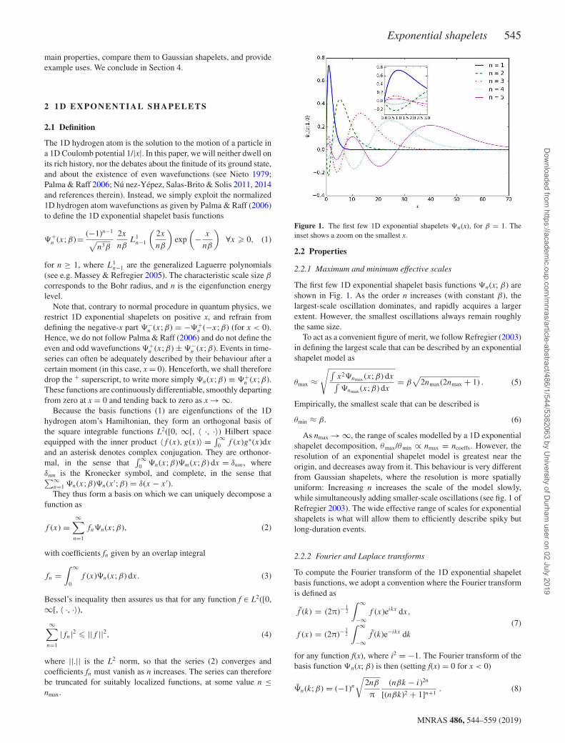
Figure 1. The first few 1D exponential shapelets �n(x), for β = 1. Theinset shows a zoom on the smallest x.
2.2 Properties
2.2.1 Maximum and minimum effective scales
The first few 1D exponential shapelet basis functions �n(x; β) areshown in Fig. 1. As the order n increases (with constant β), thelargest-scale oscillation dominates, and rapidly acquires a largerextent. However, the smallest oscillations always remain roughlythe same size.
To act as a convenient figure of merit, we follow Refregier (2003)in defining the largest scale that can be described by an exponentialshapelet model as
θmax ≈√∫
x2�nmax (x; β) dx∫�nmax (x; β) dx
= β√
2nmax(2nmax + 1) . (5)
Empirically, the smallest scale that can be described is
θmin ≈ β. (6)
As nmax → ∞, the range of scales modelled by a 1D exponentialshapelet decomposition, θmax/θmin ∝ nmax = ncoeffs. However, theresolution of an exponential shapelet model is greatest near theorigin, and decreases away from it. This behaviour is very differentfrom Gaussian shapelets, where the resolution is more spatiallyuniform: Increasing n increases the scale of the model slowly,while simultaneously adding smaller-scale oscillations (see fig. 1 ofRefregier 2003). The wide effective range of scales for exponentialshapelets is what will allow them to efficiently describe spiky butlong-duration events.
2.2.2 Fourier and Laplace transforms
To compute the Fourier transform of the 1D exponential shapeletbasis functions, we adopt a convention where the Fourier transformis defined as
f (k) = (2π)−12
∫ ∞
−∞f (x)eikx dx,
f (x) = (2π)−12
∫ ∞
−∞f (k)e−ikx dk
(7)
for any function f(x), where i2 = −1. The Fourier transform of thebasis function �n(x; β) is then (setting f(x) = 0 for x < 0)
�n(k; β) = (−1)n√
2nβ
π
(nβk − i)2n
[(nβk)2 + 1]n+1. (8)
MNRAS 486, 544–559 (2019)
Dow
nloaded from https://academ
ic.oup.com/m
nras/article-abstract/486/1/544/5382063 by University of D
urham user on 02 July 2019
546 J. Berge et al.
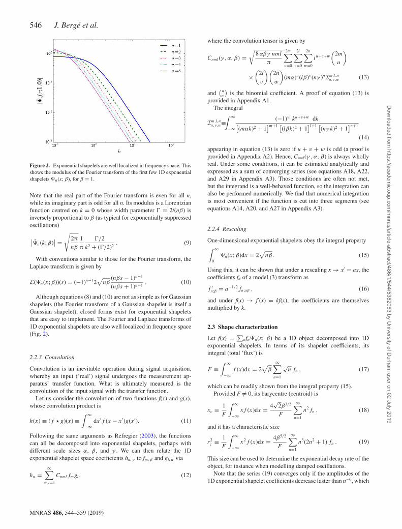
Figure 2. Exponential shapelets are well localized in frequency space. Thisshows the modulus of the Fourier transform of the first few 1D exponentialshapelets �n(x; β), for β = 1.
Note that the real part of the Fourier transform is even for all n,while its imaginary part is odd for all n. Its modulus is a Lorentzianfunction centred on k = 0 whose width parameter � ≡ 2/(nβ) isinversely proportional to β (as typical for exponentially suppressedoscillations)
∣∣�n(k; β)∣∣ =
√2π
nβ
1
π
�/2
k2 + (�/2)2. (9)
With conventions similar to those for the Fourier transform, theLaplace transform is given by
L(�n(x; β))(s) = (−1)n−12√
nβ(nβs − 1)n−1
(nβs + 1)n+1. (10)
Although equations (8) and (10) are not as simple as for Gaussianshapelets (the Fourier transform of a Gaussian shapelet is itself aGaussian shapelet), closed forms exist for exponential shapeletsthat are easy to implement. The Fourier and Laplace transforms of1D exponential shapelets are also well localized in frequency space(Fig. 2).
2.2.3 Convolution
Convolution is an inevitable operation during signal acquisition,whereby an input (‘real’) signal undergoes the measurement ap-paratus’ transfer function. What is ultimately measured is theconvolution of the input signal with the transfer function.
Let us consider the convolution of two functions f(x) and g(x),whose convolution product is
h(x) ≡ (f � g)(x) ≡∫ ∞
−∞dx ′f (x − x ′)g(x ′). (11)
Following the same arguments as Refregier (2003), the functionscan all be decomposed into exponential shapelets, perhaps withdifferent scale sizes α, β, and γ . We can then relate the 1Dexponential shapelet space coefficients hn; γ to fm; β and gl; α via
hn =∞∑
m,l=1
Cnmlfmgl, (12)
where the convolution tensor is given by
Cnml(γ, α, β) =√
8 αβγ nml
π
2m∑u=0
2l∑v=0
2n∑w=0
iu+v+w
(2m
u
)
×(
2l
v
)(2n
w
)(mα)u(lβ)v(nγ )nIm,l,n
u,v,w (13)
and(
n
m
)is the binomial coefficient. A proof of equation (13) is
provided in Appendix A1.The integral
Im,l,nu,v,w≡
∫ ∞
−∞
(−1)w ku+v+w dk[(mαk)2 + 1
]m+1 [(lβk)2 + 1
]l+1 [(nγ k)2 + 1
]n+1
(14)
appearing in equation (13) is zero if u + v + w is odd (a proof isprovided in Appendix A2). Hence, Cnml(γ , α, β) is always whollyreal. Under some conditions, it can be estimated analytically andexpressed as a sum of converging series (see equations A18, A22,and A29 in Appendix A3). Those conditions are often not met,but the integrand is a well-behaved function, so the integration canalso be performed numerically. We find that numerical integrationis most convenient if the function is cut into three segments (seeequations A14, A20, and A27 in Appendix A3).
2.2.4 Rescaling
One-dimensional exponential shapelets obey the integral property∫ ∞
0�n(x; β)dx = 2
√nβ. (15)
Using this, it can be shown that under a rescaling x → x′ = ax, thecoefficients fn of a model (3) transform as
f ′n;β = a−1/2fn;aβ , (16)
and under f(x) → f′(x) = kf(x), the coefficients are themselvesmultiplied by k.
2.3 Shape characterization
Let f(x) = ∑nfn�n(x; β) be a 1D object decomposed into 1D
exponential shapelets. In terms of its shapelet coefficients, itsintegral (total ‘flux’) is
F ≡∫ ∞
−∞f (x)dx = 2
√β
∞∑n=1
√n fn , (17)
which can be readily shown from the integral property (15).Provided F �= 0, its barycentre (centroid) is
xc ≡ 1
F
∫ ∞
−∞xf (x)dx = 4
√2β3/2
F
∞∑n=1
n2fn , (18)
and it has a characteristic size
r2c ≡ 1
F
∫ ∞
−∞x2f (x)dx = 4β5/2
F
∞∑n=1
n3(2n2 + 1) fn . (19)
This size can be used to determine the exponential decay rate of theobject, for instance when modelling damped oscillations.
Note that the series (19) converges only if the amplitudes of the1D exponential shapelet coefficients decrease faster than n−6, which
MNRAS 486, 544–559 (2019)
Dow
nloaded from https://academ
ic.oup.com/m
nras/article-abstract/486/1/544/5382063 by University of D
urham user on 02 July 2019
Exponential shapelets 547
may not always be the case. Care must therefore be taken to checkfor convergence when characterizing the shape of a feature usingthis technique.
2.4 Exponential shapelet modelling in practice
As shown above (equation 2), a 1D feature is straightforward tomodel for a given couple (nmax, β), where nmax is the maximumorder of the truncated sum (2). For example, a linear least-squaremethod can be efficiently used for this purpose. Then the modeldepends non-linearly on the two parameters nmax and β that canbe optimized by iteratively minimizing the residuals between theobserved feature and its model. This procedure was described atlength, in the 2D case, by Massey & Refregier (2005).
2.5 Example applications
This section demonstrates three possible applications of 1D expo-nential shapelets. We start by modelling exponentially suppressedoscillations, which are measurements throughout experimentalphysics, including the response of accelerometers1 onboard thespace missions MICROSCOPE (Touboul, Metris & Rodrigues2017), GRACE (Tapley et al. 2004), and GOCE (Rummel, Yi &Stummer 2011). We then discuss a potential application to un-modelled bursts in the analysis of gravitational waves. Exponentialshapelets may also be convenient to model charge transfer inef-ficiency trailing due to radiation damage in spacebourne imagingdetectors (Massey et al. 2010), although we do not explore thatfurther here.
2.5.1 Cleaning accelerometer time series data, and modelling anexperiment’s response function
MICROSCOPE tested the weak equivalence principle (WEP) byprecisely measuring the differential acceleration experienced bytwo concentric cylindrical test masses onboard a drag-free satellitein Low Earth Orbit.2 In theory, any non-zero difference at a well-defined frequency fEP (which depends on the orbit and attitudecharacteristics of the satellite) is a signature of violation of theWEP.
In practice, many transients are apparent in MICROSCOPE data(the upper panel of Fig. 3 shows a typical high-signal-to-noiseexample). These transients are generally caused by crackles ofthe satellite’s coating (because of temperature variations), cracklesof the satellite’s gas tanks (as their pressure decreases as the gasis consumed), or impacts with micro-meteorites. Such transientsoccupy frequencies higher than fEP, so they do not directly impact apossible WEP violation signal. However, it is necessary to detect andmask them in measured time-series, and then either reconstruct thecorresponding ‘missing data’ (Berge et al. 2015; Pires et al. 2016) toallow for a least-square fit of the expected WEP violation signal inthe frequency domain (Touboul et al. 2017), or adapt the maximumlikelihood technique to take missing data into account (Baghi et al.2015, 2016). Existing techniques are suboptimal, as they may affectthe noise characteristics. Moreover, transients could be consideredas conveying useful information. They are created by an externalimpulse; if this is assumed to be instantaneous (Dirac), the shape
1http://www.onera.fr/en/dphy2The mission ended on 2018 October 16; data analysis is still underway.
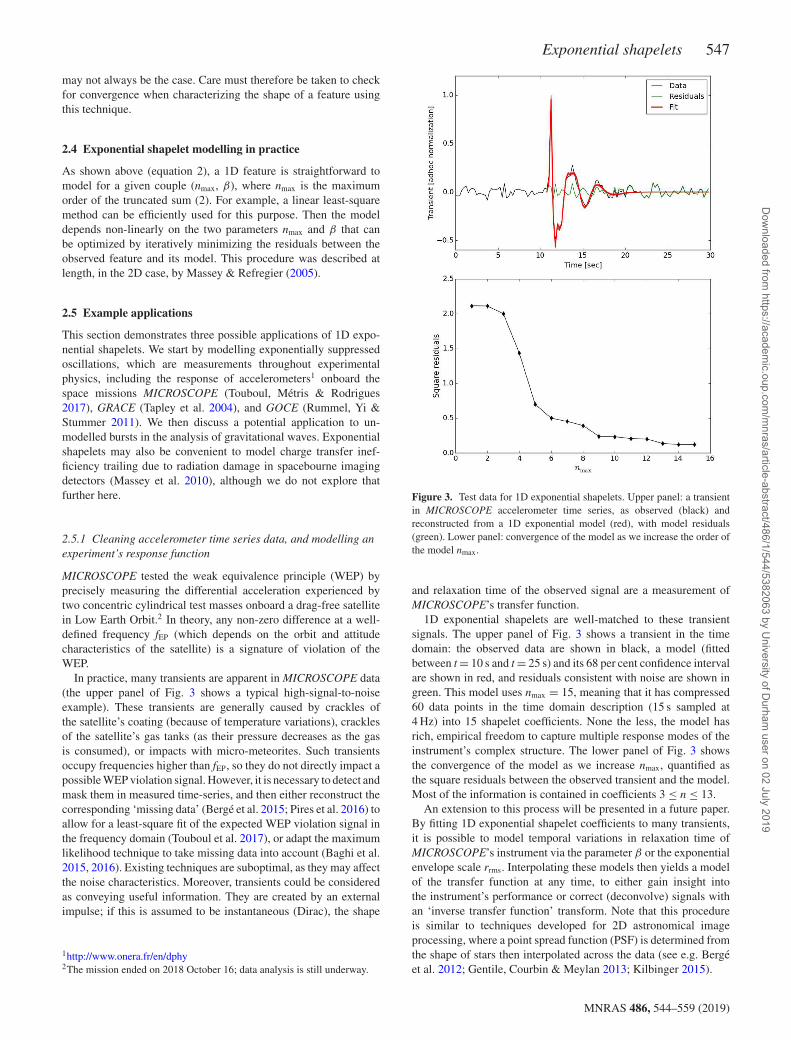
Figure 3. Test data for 1D exponential shapelets. Upper panel: a transientin MICROSCOPE accelerometer time series, as observed (black) andreconstructed from a 1D exponential model (red), with model residuals(green). Lower panel: convergence of the model as we increase the order ofthe model nmax.
and relaxation time of the observed signal are a measurement ofMICROSCOPE’s transfer function.
1D exponential shapelets are well-matched to these transientsignals. The upper panel of Fig. 3 shows a transient in the timedomain: the observed data are shown in black, a model (fittedbetween t = 10 s and t = 25 s) and its 68 per cent confidence intervalare shown in red, and residuals consistent with noise are shown ingreen. This model uses nmax = 15, meaning that it has compressed60 data points in the time domain description (15 s sampled at4 Hz) into 15 shapelet coefficients. None the less, the model hasrich, empirical freedom to capture multiple response modes of theinstrument’s complex structure. The lower panel of Fig. 3 showsthe convergence of the model as we increase nmax, quantified asthe square residuals between the observed transient and the model.Most of the information is contained in coefficients 3 ≤ n ≤ 13.
An extension to this process will be presented in a future paper.By fitting 1D exponential shapelet coefficients to many transients,it is possible to model temporal variations in relaxation time ofMICROSCOPE’s instrument via the parameter β or the exponentialenvelope scale rrms. Interpolating these models then yields a modelof the transfer function at any time, to either gain insight intothe instrument’s performance or correct (deconvolve) signals withan ‘inverse transfer function’ transform. Note that this procedureis similar to techniques developed for 2D astronomical imageprocessing, where a point spread function (PSF) is determined fromthe shape of stars then interpolated across the data (see e.g. Bergeet al. 2012; Gentile, Courbin & Meylan 2013; Kilbinger 2015).
MNRAS 486, 544–559 (2019)
Dow
nloaded from https://academ
ic.oup.com/m
nras/article-abstract/486/1/544/5382063 by University of D
urham user on 02 July 2019
548 J. Berge et al.
2.5.2 Characterization of perturbing signals in space-bornegeodesy missions
The GRACE mission (Tapley et al. 2004) revolutionized geodesyby measuring the Earth’s gravitational field with unprecedentedprecision. Two satellites followed each other on the same orbit,monitoring the distance between them via microwave ranging. Intheory, any variation in their relative speed or distance can beascribed to variations in the Earth’s geopotential.
In practice, the satellites were also subject to non-gravitationalforces. These were measured by ultrasensitive accelerometers, forremoval during post-processing (Flury et al. 2008; Peterseim et al.2010). Peterseim (2014) and Peterseim et al. (2014) modelled tran-sients (known as ‘spikes’) in accelerometer data using a piecewisefunction made from the derivative of a Gaussian, a third-orderpolynomial, and a damped oscillation. Some were successfullyclassified as either due to the satellite’s heaters or due to activationof its magnetic torquers – but no physical origin could be assignedto others, known as ‘twangs’.
Tentative correlations of twangs with the position of the satellitealong its orbit hint at a possible geophysical origin. Both categoriesof twangs are compactly represented as 1D exponential shapelets,so we will investigate in a future paper whether these provide acleaner set of shape parameters to categorize and understand theirorigin.
2.5.3 Unmodelled bursts and glitches in gravitational wave dataanalysis
A wealth of methods have been developed to search for, charac-terize, and classify unmodelled bursts and instrumental glitchesin searches for gravitational waves (see e.g. Cornish & Litten-berg 2015; Powell et al. 2015, 2017; Principe & Pinto 2017,and references therein). Glitches are often modelled using ‘sine-Gaussian waveforms’ (Principe & Pinto 2017). These have similarproperties to Gaussian shapelets, although shapelets can encodemore details. One-dimensional exponential shapelets could furtheroptimize the data compression of complex glitch shapes that oftenexhibit damped oscillations.
Shapelets might therefore improve the detection, characteriza-tion, and classification of instrumental glitches in gravitational wavedetectors. Indeed, bursts and glitches are usually detected in thetime–frequency domain, which is easily reproduced in Gaussianshapelet-time space. If 1D exponential shapelets more efficientlymodel the information in a glitch, exponential shapelet-time spacewould be even better. We will investigate in a future paper whetherglitches can be detected by scanning a matched filter and correlatingthe measured signal with a 1D exponential shapelet model whileleaving β (and possibly nmax) free.
2.6 Comparison with Gaussian shapelets
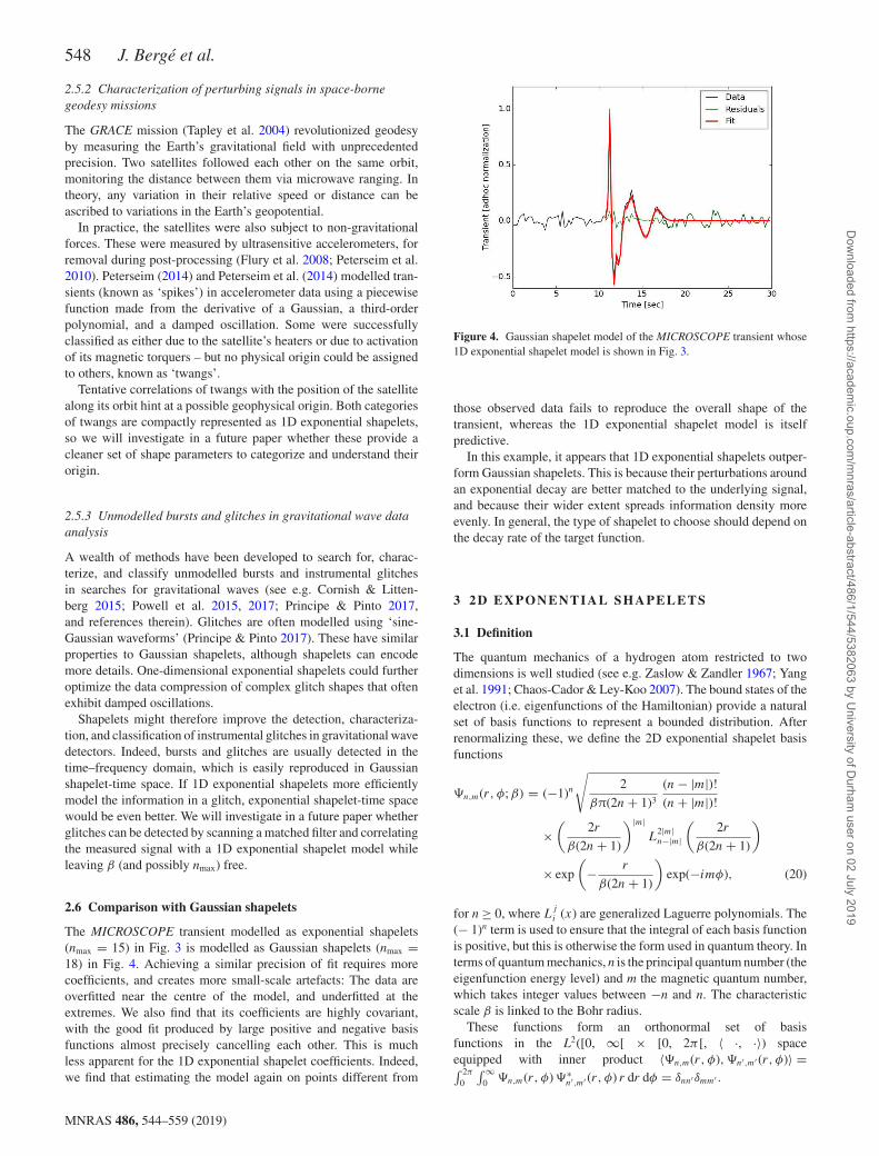
The MICROSCOPE transient modelled as exponential shapelets(nmax = 15) in Fig. 3 is modelled as Gaussian shapelets (nmax =18) in Fig. 4. Achieving a similar precision of fit requires morecoefficients, and creates more small-scale artefacts: The data areoverfitted near the centre of the model, and underfitted at theextremes. We also find that its coefficients are highly covariant,with the good fit produced by large positive and negative basisfunctions almost precisely cancelling each other. This is muchless apparent for the 1D exponential shapelet coefficients. Indeed,we find that estimating the model again on points different from
Figure 4. Gaussian shapelet model of the MICROSCOPE transient whose1D exponential shapelet model is shown in Fig. 3.
those observed data fails to reproduce the overall shape of thetransient, whereas the 1D exponential shapelet model is itselfpredictive.
In this example, it appears that 1D exponential shapelets outper-form Gaussian shapelets. This is because their perturbations aroundan exponential decay are better matched to the underlying signal,and because their wider extent spreads information density moreevenly. In general, the type of shapelet to choose should depend onthe decay rate of the target function.
3 2 D EXPONENTI AL SHAPELETS
3.1 Definition
The quantum mechanics of a hydrogen atom restricted to twodimensions is well studied (see e.g. Zaslow & Zandler 1967; Yanget al. 1991; Chaos-Cador & Ley-Koo 2007). The bound states of theelectron (i.e. eigenfunctions of the Hamiltonian) provide a naturalset of basis functions to represent a bounded distribution. Afterrenormalizing these, we define the 2D exponential shapelet basisfunctions
�n,m(r, φ; β) = (−1)n√
2
βπ(2n + 1)3
(n − |m|)!(n + |m|)!
×(
2r
β(2n + 1)
)|m|L
2|m|n−|m|
(2r
β(2n + 1)
)
× exp
(− r
β(2n + 1)
)exp(−imφ), (20)
for n ≥ 0, where Lj
i (x) are generalized Laguerre polynomials. The(− 1)n term is used to ensure that the integral of each basis functionis positive, but this is otherwise the form used in quantum theory. Interms of quantum mechanics, n is the principal quantum number (theeigenfunction energy level) and m the magnetic quantum number,which takes integer values between −n and n. The characteristicscale β is linked to the Bohr radius.
These functions form an orthonormal set of basisfunctions in the L2([0, ∞[ × [0, 2π [, 〈 ·, ·〉) spaceequipped with inner product 〈�n,m(r, φ), �n′,m′ (r, φ)〉 =∫ 2π
0
∫ ∞0 �n,m(r, φ) �∗
n′,m′ (r, φ) r dr dφ = δnn′δmm′ .
MNRAS 486, 544–559 (2019)
Dow
nloaded from https://academ
ic.oup.com/m
nras/article-abstract/486/1/544/5382063 by University of D
urham user on 02 July 2019
Exponential shapelets 549
Any localized function f(r, φ) can be uniquely decomposed intoa weighted sum of these basis functions
f (r, φ) =∞∑
n=0
n∑m=−n
fn,m �n,m(r, φ; β), (21)
where the 2D exponential shapelet coefficients are given by
fn,m =∫ 2π
0
∫ ∞
0f (r, φ) �n,m(r, φ; β) r dr dφ. (22)
Using Bessel’s inequality like in the 1D case, we find that series(21) converges, and the coefficients fn,m must vanish when n andm increase. For a real function f (r, φ) ∈ R, fn,m = f ∗
n−m. In thiscase, truncating the series at n ≤ nmax results in ncoeffs = (nmax + 1)2
independent coefficients.It may also be possible to define elliptical 2D exponential
shapelets by applying a shear transformation to the coordinatesystem, as Nakajima & Bernstein (2007) suggested for Gaussianshapelets. This preserves their orthonormality, and can increasetheir rate of data compression, at the cost of two additional non-linear parameters to specify the shear.
3.2 Properties
3.2.1 Maximum and minimum effective scales
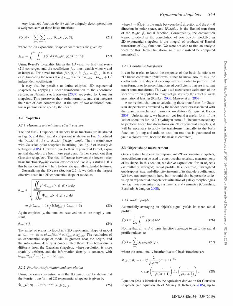
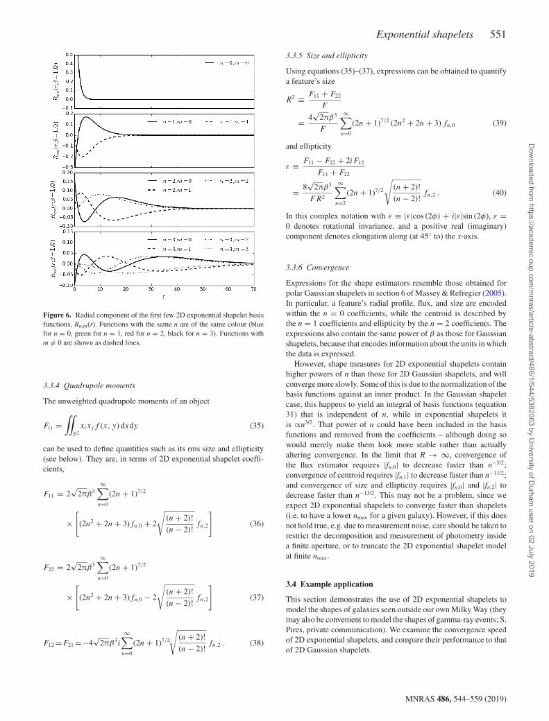
The first few 2D exponential shapelet basis functions are illustratedin Fig. 5, and their radial component is shown in Fig. 6, definedvia �n,m(r, φ; β) ≡ Rn,m(r; β)exp (−imφ). Their resemblancewith Gaussian polar shapelets is striking (see fig. 2 of Massey &Refregier 2005). However, due to their exponential kernel, expo-nential shapelets are both more peaky and further spread out thanGaussian shapelets. The size difference between the lowest-orderbasis function �00 and even a low-order one like �40 is striking. It isthis behaviour that will help to describe spatially extended features.
Generalizing the 1D case (Section 2.2.1), we define the largesteffective scale in a 2D exponential shapelet model as
θmax ≈
√√√√√√√√“
R2r2 �nmax,0(r, φ; β) rdrdφ
“R2
�nmax,0(r, φ; β) rdrdφ
= β(2nmax + 1)√
2(2n2max + 2nmax + 3) . (23)
Again empirically, the smallest resolved scales are roughly con-stant,
θmin ≈ β. (24)
The range of scales included in a 2D exponential shapelet modelas nmax → ∞ is (θmax/θmin)2 ∝ n4
max ∝ n2coeffs. The resolution of
an exponential shapelet model is greatest near the origin, andthe information density is concentrated there. This behaviour isdifferent from the Gaussian shapelets, where resolution is morespatially uniform, and the information density is constant, with(θmax/θmin)2 = n2
max + 1 ∝ ncoeffs.
3.2.2 Fourier transformation and convolution
Using the same convention as in the 1D case, it can be shown thatthe Fourier transform of 2D exponential shapelets is given by
�n,m(�k; β) = 2πime−imφk [Fm(k)]n,β , (25)
where k = |�k|, φk is the angle between the �k direction and the φ = 0direction in polar space, and [Fm(k)]n,β is the Hankel transformof the Rnm(r, β) radial function. Consequently, the convolutiontensor involved in the convolution of two objects modelled in2D exponential shapelets is the integral of products of Hankeltransforms of Rn,m functions. We were not able to find an analyticform for this Hankel transform, so it must instead be computednumerically.
3.2.3 Coordinate transforms
It can be useful to know the response of the basis functions to2D linear coordinate transforms: either to know how to mix thecoefficients of a shapelet decomposition in order to perform thattransform, or to form combinations of coefficients that are invariantunder some transforms. This was used to construct estimators of theshear distortion applied to images of galaxies by the effect of weakgravitational lensing (Kuijken 2006; Massey et al. 2007).
A convenient shortcut to calculating those transforms for Gaus-sian shapelets was provided by the ladder operators associated withthe quantum mechanical harmonic oscillator (Refregier & Bacon2003). Unfortunately, we have not yet found a useful form of theladder operators for the 2D hydrogen atom. If it becomes necessaryto perform linear transformations on 2D exponential shapelets, itwill be necessary to apply the transforms manually to the basisfunctions (a long and arduous task, but one that is guaranteed toyield a closed form, because the basis is complete).
3.3 Object shape measurement
Once a feature has been decomposed into 2D exponential shapelets,its coefficients can be used to construct characteristic measurementsof its shape. In this section, we derive expressions for an object’s(azimuthally averaged) radial profile, flux, centroid, unweightedquadrupoles, size, and ellipticity, in terms of its shapelet coefficients.We have not attempted it here, but it should also be possible to de-velop an exponential-shapelet classification of galaxy morphologiesvia e.g. their concentration, asymmetry, and symmetry (Conselice,Bershady & Jangren 2000).
3.3.1 Radial profile
Azimuthally averaging an object’s signal yields its mean radialprofile
f (r) ≡ 1
2π
∫ 2π
0f (r, φ) dφ. (26)
Noting that all m �= 0 basis functions average to zero, the radialprofile reduces to
f (r) =∞∑
n=0
fn,0�n,0(r; β), (27)
where the (rotationally invariant) m = 0 basis functions are
�n,0(r; β) = (−1)n2
β√
2π(2n + 1)−3/2
× exp
(− r
β(2n + 1)
)Ln
(r
β(n + 12 )
). (28)
Equation (26) is identical to the equivalent derivation for Gaussianshapelets (see equation 16 of Massey & Refregier 2005), up to
MNRAS 486, 544–559 (2019)
Dow
nloaded from https://academ
ic.oup.com/m
nras/article-abstract/486/1/544/5382063 by University of D
urham user on 02 July 2019
550 J. Berge et al.
Figure 5. The first few 2D exponential shapelet basis functions: real part (left) and imaginary part (right). Red is positive; blue is negative. The normalizationof both the colour scale and the spatial scale is arbitrary, but is the same in every box.
the fact that m = 0 basis functions with odd n do not exist in theGaussian case.
3.3.2 Flux
Integrating the signal inside a circular aperture of radius R yieldsits ‘flux’
FR ≡∫ 2π
0
∫ R
0f (r, φ) r dr dφ. (29)
To evaluate this integral, it is useful to note that, once again, all m �=0 basis functions cancel out to zero during integration over φ, andalso a closed form for the generalized Laguerre polynomials,
Lαn (x) =
n∑k=0
(−1)k(
n + α
n − k
)xk
k!. (30)
Using this, it can be shown that
FR = 2√
2πβ
∞∑n=0
fn,0 (2n + 1)1/2
×n∑
k=0
2k(−1)n+k
k!
(n
k
)γ
(k + 2,
R
β(2n + 1)
), (31)
where γ (y, x) is the lower incomplete gamma function. Extrapolat-ing FR to a large radius, and taking the limit R → ∞, we obtain
F ≡“
R2f (r, φ) rdrdφ = 2
√2πβ
∞∑n=0
(2n + 1)3/2fn,0 . (32)
3.3.3 Centroid
Similarly, it can be shown that the unweighted centroid (xc, yc),defined by
xc + iyc ≡
“R2
(x + iy)f (x, y) dxdy
“R2
f (x, y) dxdy
, (33)
is, in terms of 2D exponential shapelet coefficients,
xc + iyc = −4√
2πβ2
F
∞∑n=1
√n(n + 1)(2n + 1)5 fn,1 . (34)
MNRAS 486, 544–559 (2019)
Dow
nloaded from https://academ
ic.oup.com/m
nras/article-abstract/486/1/544/5382063 by University of D
urham user on 02 July 2019
Exponential shapelets 551
Figure 6. Radial component of the first few 2D exponential shapelet basisfunctions, Rn,m(r). Functions with the same n are of the same colour (bluefor n = 0, green for n = 1, red for n = 2, black for n = 3). Functions withm �= 0 are shown as dashed lines.
3.3.4 Quadrupole moments
The unweighted quadrupole moments of an object
Fij =“
R2xixjf (x, y) dxdy (35)
can be used to define quantities such as its rms size and ellipticity(see below). They are, in terms of 2D exponential shapelet coeffi-cients,
F11 = 2√
2πβ3∞∑
n=0
(2n + 1)7/2
×[
(2n2 + 2n + 3)fn,0 + 2
√(n + 2)!
(n − 2)!fn,2
](36)
F22 = 2√
2πβ3∞∑
n=0
(2n + 1)7/2
×[
(2n2 + 2n + 3)fn,0 − 2
√(n + 2)!
(n − 2)!fn,2
](37)
F12 =F21 =−4√
2πβ3i
∞∑n=0
(2n + 1)7/2
√(n + 2)!
(n − 2)!fn,2 . (38)
3.3.5 Size and ellipticity
Using equations (35)–(37), expressions can be obtained to quantifya feature’s size
R2 ≡ F11 + F22
F
= 4√
2πβ3
F
∞∑n=0
(2n + 1)7/2 (2n2 + 2n + 3) fn,0 (39)
and ellipticity
ε ≡ F11 − F22 + 2iF12
F11 + F22
= 8√
2πβ3
FR2
∞∑n=2
(2n + 1)7/2
√(n + 2)!
(n − 2)!fn,2 . (40)
In this complex notation with ε ≡ |ε|cos (2φ) + i|ε|sin (2φ), ε =0 denotes rotational invariance, and a positive real (imaginary)component denotes elongation along (at 45◦ to) the x-axis.
3.3.6 Convergence
Expressions for the shape estimators resemble those obtained forpolar Gaussian shapelets in section 6 of Massey & Refregier (2005).In particular, a feature’s radial profile, flux, and size are encodedwithin the n = 0 coefficients, while the centroid is described bythe n = 1 coefficients and ellipticity by the n = 2 coefficients. Theexpressions also contain the same power of β as those for Gaussianshapelets, because that encodes information about the units in whichthe data is expressed.
However, shape measures for 2D exponential shapelets containhigher powers of n than those for 2D Gaussian shapelets, and willconverge more slowly. Some of this is due to the normalization of thebasis functions against an inner product. In the Gaussian shapeletcase, this happens to yield an integral of basis functions (equation31) that is independent of n, while in exponential shapelets itis ∝n3/2. That power of n could have been included in the basisfunctions and removed from the coefficients – although doing sowould merely make them look more stable rather than actuallyaltering convergence. In the limit that R → ∞, convergence ofthe flux estimator requires |fn,0| to decrease faster than n−5/2;convergence of centroid requires |fn,1| to decrease faster than n−11/2;and convergence of size and ellipticity requires |fn,0| and |fn,2| todecrease faster than n−13/2. This may not be a problem, since weexpect 2D exponential shapelets to converge faster than shapelets(i.e. to have a lower nmax for a given galaxy). However, if this doesnot hold true, e.g. due to measurement noise, care should be taken torestrict the decomposition and measurement of photometry insidea finite aperture, or to truncate the 2D exponential shapelet modelat finite nmax.
3.4 Example application
This section demonstrates the use of 2D exponential shapelets tomodel the shapes of galaxies seen outside our own Milky Way (theymay also be convenient to model the shapes of gamma-ray events; S.Pires, private communication). We examine the convergence speedof 2D exponential shapelets, and compare their performance to thatof 2D Gaussian shapelets.
MNRAS 486, 544–559 (2019)
Dow
nloaded from https://academ
ic.oup.com/m
nras/article-abstract/486/1/544/5382063 by University of D
urham user on 02 July 2019
552 J. Berge et al.
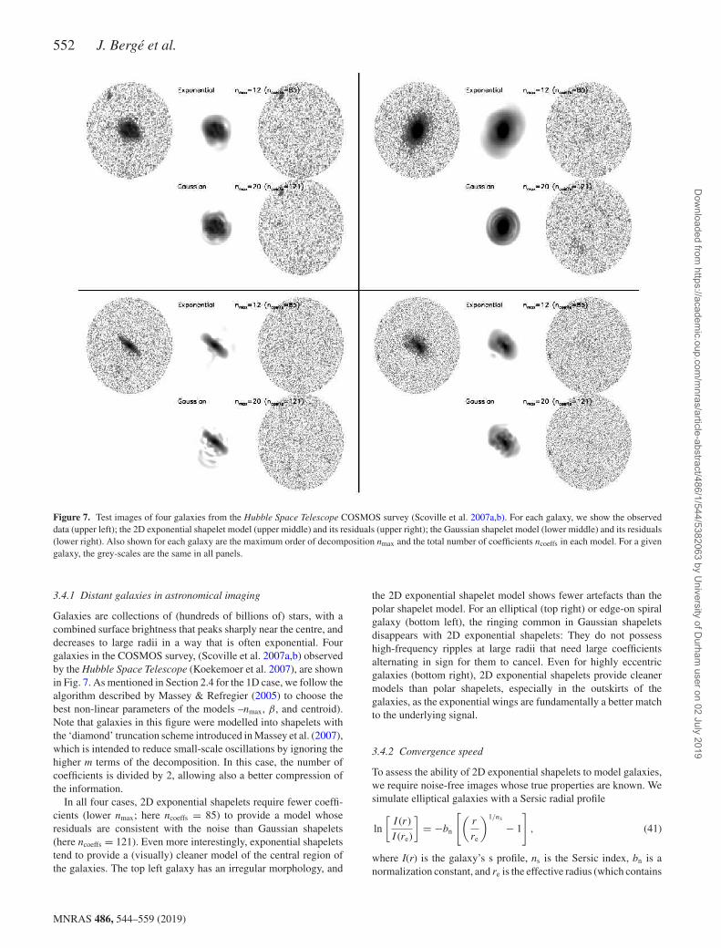
Figure 7. Test images of four galaxies from the Hubble Space Telescope COSMOS survey (Scoville et al. 2007a,b). For each galaxy, we show the observeddata (upper left); the 2D exponential shapelet model (upper middle) and its residuals (upper right); the Gaussian shapelet model (lower middle) and its residuals(lower right). Also shown for each galaxy are the maximum order of decomposition nmax and the total number of coefficients ncoeffs in each model. For a givengalaxy, the grey-scales are the same in all panels.
3.4.1 Distant galaxies in astronomical imaging
Galaxies are collections of (hundreds of billions of) stars, with acombined surface brightness that peaks sharply near the centre, anddecreases to large radii in a way that is often exponential. Fourgalaxies in the COSMOS survey, (Scoville et al. 2007a,b) observedby the Hubble Space Telescope (Koekemoer et al. 2007), are shownin Fig. 7. As mentioned in Section 2.4 for the 1D case, we follow thealgorithm described by Massey & Refregier (2005) to choose thebest non-linear parameters of the models –nmax, β, and centroid).Note that galaxies in this figure were modelled into shapelets withthe ‘diamond’ truncation scheme introduced in Massey et al. (2007),which is intended to reduce small-scale oscillations by ignoring thehigher m terms of the decomposition. In this case, the number ofcoefficients is divided by 2, allowing also a better compression ofthe information.
In all four cases, 2D exponential shapelets require fewer coeffi-cients (lower nmax; here ncoeffs = 85) to provide a model whoseresiduals are consistent with the noise than Gaussian shapelets(here ncoeffs = 121). Even more interestingly, exponential shapeletstend to provide a (visually) cleaner model of the central region ofthe galaxies. The top left galaxy has an irregular morphology, and
the 2D exponential shapelet model shows fewer artefacts than thepolar shapelet model. For an elliptical (top right) or edge-on spiralgalaxy (bottom left), the ringing common in Gaussian shapeletsdisappears with 2D exponential shapelets: They do not possesshigh-frequency ripples at large radii that need large coefficientsalternating in sign for them to cancel. Even for highly eccentricgalaxies (bottom right), 2D exponential shapelets provide cleanermodels than polar shapelets, especially in the outskirts of thegalaxies, as the exponential wings are fundamentally a better matchto the underlying signal.
3.4.2 Convergence speed
To assess the ability of 2D exponential shapelets to model galaxies,we require noise-free images whose true properties are known. Wesimulate elliptical galaxies with a Sersic radial profile
ln
[I (r)
I (re)
]= −bn
[(r
re
)1/ns
− 1
], (41)
where I(r) is the galaxy’s s profile, ns is the Sersic index, bn is anormalization constant, and re is the effective radius (which contains
MNRAS 486, 544–559 (2019)
Dow
nloaded from https://academ
ic.oup.com/m
nras/article-abstract/486/1/544/5382063 by University of D
urham user on 02 July 2019
Exponential shapelets 553
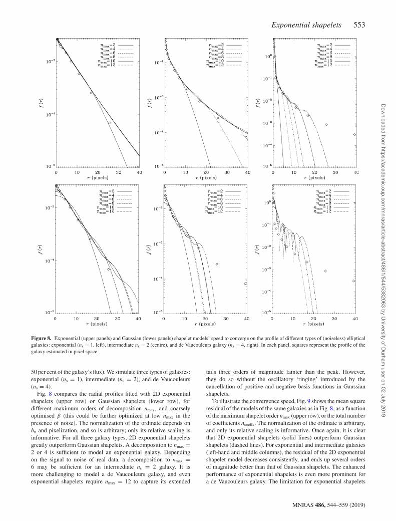
Figure 8. Exponential (upper panels) and Gaussian (lower panels) shapelet models’ speed to converge on the profile of different types of (noiseless) ellipticalgalaxies: exponential (ns = 1, left), intermediate ns = 2 (centre), and de Vaucouleurs galaxy (ns = 4, right). In each panel, squares represent the profile of thegalaxy estimated in pixel space.
50 per cent of the galaxy’s flux). We simulate three types of galaxies:exponential (ns = 1), intermediate (ns = 2), and de Vaucouleurs(ns = 4).
Fig. 8 compares the radial profiles fitted with 2D exponentialshapelets (upper row) or Gaussian shapelets (lower row), fordifferent maximum orders of decomposition nmax, and coarselyoptimised β (this could be further optimized at low nmax in thepresence of noise). The normalization of the ordinate depends onbn and pixelization, and so is arbitrary; only its relative scaling isinformative. For all three galaxy types, 2D exponential shapeletsgreatly outperform Gaussian shapelets. A decomposition to nmax =2 or 4 is sufficient to model an exponential galaxy. Dependingon the signal to noise of real data, a decomposition to nmax =6 may be sufficient for an intermediate ns = 2 galaxy. It ismore challenging to model a de Vaucouleurs galaxy, and evenexponential shapelets require nmax = 12 to capture its extended
tails three orders of magnitude fainter than the peak. However,they do so without the oscillatory ‘ringing’ introduced by thecancellation of positive and negative basis functions in Gaussianshapelets.
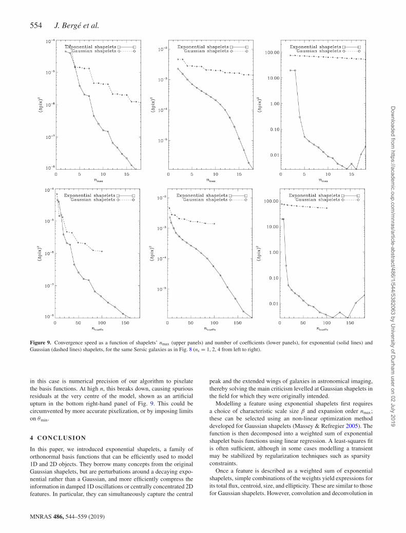
To illustrate the convergence speed, Fig. 9 shows the mean squareresidual of the models of the same galaxies as in Fig. 8, as a functionof the maximum shapelet order nmax (upper row), or the total numberof coefficients ncoeffs. The normalization of the ordinate is arbitrary,and only its relative scaling is informative. Once again, it is clearthat 2D exponential shapelets (solid lines) outperform Gaussianshapelets (dashed lines). For exponential and intermediate galaxies(left-hand and middle columns), the residual of the 2D exponentialshapelet model decreases consistently, and ends up several ordersof magnitude better than that of Gaussian shapelets. The enhancedperformance of exponential shapelets is even more prominent fora de Vaucouleurs galaxy. The limitation for exponential shapelets
MNRAS 486, 544–559 (2019)
Dow
nloaded from https://academ
ic.oup.com/m
nras/article-abstract/486/1/544/5382063 by University of D
urham user on 02 July 2019
554 J. Berge et al.
Figure 9. Convergence speed as a function of shapelets’ nmax (upper panels) and number of coefficients (lower panels), for exponential (solid lines) andGaussian (dashed lines) shapelets, for the same Sersic galaxies as in Fig. 8 (ns = 1, 2, 4 from left to right).
in this case is numerical precision of our algorithm to pixelatethe basis functions. At high n, this breaks down, causing spuriousresiduals at the very centre of the model, shown as an artificialupturn in the bottom right-hand panel of Fig. 9. This could becircumvented by more accurate pixelization, or by imposing limitson θmin.
4 C O N C L U S I O N
In this paper, we introduced exponential shapelets, a family oforthonormal basis functions that can be efficiently used to model1D and 2D objects. They borrow many concepts from the originalGaussian shapelets, but are perturbations around a decaying expo-nential rather than a Gaussian, and more efficiently compress theinformation in damped 1D oscillations or centrally concentrated 2Dfeatures. In particular, they can simultaneously capture the central
peak and the extended wings of galaxies in astronomical imaging,thereby solving the main criticism levelled at Gaussian shapelets inthe field for which they were originally intended.
Modelling a feature using exponential shapelets first requiresa choice of characteristic scale size β and expansion order nmax;these can be selected using an non-linear optimization methoddeveloped for Gaussian shapelets (Massey & Refregier 2005). Thefunction is then decomposed into a weighted sum of exponentialshapelet basis functions using linear regression. A least-squares fitis often sufficient, although in some cases modelling a transientmay be stabilized by regularization techniques such as sparsityconstraints.
Once a feature is described as a weighted sum of exponentialshapelets, simple combinations of the weights yield expressions forits total flux, centroid, size, and ellipticity. These are similar to thosefor Gaussian shapelets. However, convolution and deconvolution in
MNRAS 486, 544–559 (2019)
Dow
nloaded from https://academ
ic.oup.com/m
nras/article-abstract/486/1/544/5382063 by University of D
urham user on 02 July 2019
Exponential shapelets 555
exponential shapelets are significantly more difficult than in theGaussian case, with the convolution tensor being time-consumingto calculate via numerical integration.
We described possible applications of exponential shapelets inseveral fields of experimental and observational science. One-dimensional exponential shapelets can be used to model (andsubtract or understand) spurious transients in time-series, such asmeasurements by the MICROSCOPE or GRACE satellites, or theLIGO search for gravitational waves. Thanks to their exponentialdecay, 2D exponential shapelets overcome the main criticism aimedat Gaussian shapelets (though at the cost of losing some simplicity)and can be used to measure the brightness, shape, and size of distantgalaxies in astronomical imaging. The characteristics of exponentialshapelets should make them well suited to data compression andanalysis in a wide range of fields; their convenient mathematicalproperties should see them frequently adopted.
AC K N OW L E D G E M E N T S
The concepts in this paper matured over many years, after apreliminary study to generalize Gaussian polar shapelets for HubbleSpace Telescope data, for which we acknowledge support fromNASA through grant HST-AR-11747 – and which was carried outat the Jet Propulsion Laboratory, California Institute of Technology,under a contract with NASA. We are indebted to Barnaby Rowe forresearching Kummer functions and the literature of the 2D hydrogenatom. We also acknowledge helpful and motivating discussionswith Jason Rhodes, Richard Ellis, Alexandre Refregier, SandrinePires, James Nightingale, Bernard Foulon, Bruno Christophe, GillesMetris, Manuel Rodrigues, Alain Robert, and Nicolas Touquoy. Thiswork makes use of technical data from the CNES-ESA-ONERA-CNRS-OCA Microscope mission, and has received financial sup-port from ONERA and CNES. JB acknowledges the financialsupport of the UnivEarthS Labex programme at Sorbonne Paris Cite(ANR-10-LABX-0023 and ANR-11-IDEX-0005-02) and of CNESthrough the APR programme (LISA project). RM is supported by aRoyal Society University Research Fellowship and through STFCgrant ST/N001494/1.
RE FERENCES
Akdeniz T. J., Lizotte D., Mohieddin Abukhdeir N., 2018, IOP Nanotech-nology, 30, 075703
Amara A., Quanz S. P., 2012, MNRAS, 427, 948Apostolopoulos G., Koutras A., Christoyianni I., Dermatas E., 2017, IEEE
25th European Signal Processing Conference (EUSIPCO). IEEE, p. 56Baghi Q., Metris G., Berge J., Christophe B., Touboul P., Rodrigues M.,
2015, Phys. Rev. D, 91, 062003Baghi Q., Metris G., Berge J., Christophe B., Touboul P., Rodrigues M.,
2016, Phys. Rev. D, 93, 122007Berge J., Price S., Amara A., Rhodes J., 2012, MNRAS, 419, 2356Berge J., Pires S., Baghi Q., Touboul P., Metris G., 2015, Phys. Rev. D, 92,
112006Bernstein G. M., Jarvis M., 2002, AJ, 123, 583Bezrodnykh S. I., 2016, Math. Notes, 100, 318Birrer S., Amara A., Refregier A., 2015, ApJ, 813, 102Chaos-Cador L., Ley-Koo E., 2007, Int. J. Quantum Chem., 107, 12Conselice C. J., Bershady M. A., Jangren A., 2000, ApJ, 529, 886
Cornish N. J., Littenberg T. B., 2015, Class. Quantum Gravity, 32, 135012Desvignes G. et al., 2016, MNRAS, 458, 3341Ellis J. A., Cornish N. J., 2016, Phys. Rev. D, 93, 084048Flury J., Bettadpur S., Tapley B. D., 2008, Adv. Space Res., 42, 1414Gentile M., Courbin F., Meylan G., 2013, A&A, 549, A1Hasanov A., Srivastava H. M., 2007, Comput. Math. Appl., 53, 1119Hoekstra H., Wu Y., Udalski A., 2005, ApJ, 626, 1070Holbrey R., 2006, Dimension Reduction Algorithms for Data Mining and
Visualization. University of Leeds, EdinburghJimenez-Teja Y., Benıtez N., 2012, ApJ, 745, 150Kilbinger M., 2015, Rep. Prog. Phys., 78, 086901Koekemoer A. M. et al., 2007, ApJS, 172, 196Kuijken K., 2006, A&A, 456, 827Lentati L., Alexander P., Hobson M. P., 2015, MNRAS, 447, 2159Massey R., Refregier A., 2005, MNRAS, 363, 197Massey R., Rowe B., Refregier A., Bacon D. J., Berge J., 2007, MNRAS,
380, 229Massey R., Stoughton C., Leauthaud A., Rhodes J., Koekemoer A., Ellis R.,
Shaghoulian E., 2010, MNRAS, 401, 371Melchior P., Bohnert A., Lombardi M., Bartelmann M., 2010, A&A, 510,
A75Nakajima R., Bernstein G., 2007, AJ, 133, 1763Ngan W., van Waerbeke L., Mahdavi A., Heymans C., Hoekstra H., 2009,
MNRAS, 396, 1211Nieto M. M., 1979, Am. J. Phys., 47, 1067Nu nez-Yepez H. N., Salas-Brito A. L., Solis D. A., 2011, Phys. Rev. A, 83,
064101Nu nez-Yepez H. N., Salas-Brito A. L., Solis D. A., 2014, Phys. Rev. A, 89,
049908Palma G., Raff U., 2006, Can. J. Phys., 84, 787Peterseim N., 2014, PhD Thesis. Technische Universitat, MunchenPeterseim N., Jakob F., Schlicht A., 2010, 38th COSPAR Scientific Assem-
bly, 38, 4Peterseim N., Schlicht A., Flury J., Dahle C., 2014, in Flechtner F., Sneeuw
N., Schuh W., eds, Identification and Reduction of Satellite-InducedSignals in GRACE Accelerometer Data; Observation of the SystemEarth from Space - CHAMP, GRACE, GOCE and Future Missions.GEOTECHNOLOGIEN Science Report No. 20 , Vol. 2014. Springer,p. 53
Pires S., Berge J., Baghi Q., Touboul P., Metris G., 2016, Phys. Rev. D, 94,123015
Powell J., Trifiro D., Cuoco E., Heng I. S., Cavaglia M., 2015, Class.Quantum Gravity, 32, 215012
Powell J., Torres-Forne A., Lynch R., Trifiro D., Cuoco E., Cavaglia M.,Heng I. S., Font J. A., 2017, Class. Quantum Gravity, 34, 034002
Principe M., Pinto I. M., 2017, Phys. Rev. D, 95, 082006Refregier A., 2003, MNRAS, 338, 35Refregier A., Bacon D., 2003, MNRAS, 338, 48Rummel R., Yi W., Stummer C., 2011, J. Geod., 85, 777Sabzmeydani P., Mori G., 2007, IEEE Conference on Computer Vision and
Pattern Recognition, Vol. 1, p. 90Scoville N. et al., 2007a, ApJS, 172, 1Scoville N. et al., 2007b, ApJS, 172, 38Sharpee T. O., Victor J. D., 2009, J. Comput Neurosci, 26, 203Suderman R., Lizotte D. J., Abukhdeir N. M., 2015, Phys. Rev. E, 91, 033307Tagore A. S., Jackson N., 2016, MNRAS, 457, 3066Tapley B. D., Bettadpur S., Watkins M., Reigber C., 2004, Geophys. Res.
Lett., 31, L09607Touboul P. et al., 2017, Phys. Rev. Lett., 119, 231101Weissman J., Hancewicz T., Kaplan P., 2004, Opt. Express, 12, 5760Yang X. L., Guo S. H., Chan F. T., Wong K. W., Ching W. Y., 1991, Phys.
Rev. A, 43, 1186Zaslow B., Zandler M. E., 1967, Am. J. Phys., 35, 1118
MNRAS 486, 544–559 (2019)
Dow
nloaded from https://academ
ic.oup.com/m
nras/article-abstract/486/1/544/5382063 by University of D
urham user on 02 July 2019

556 J. Berge et al.
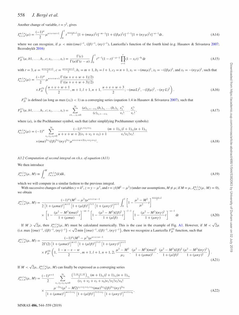
APPENDIX A : D ERIVATION O F C ONVO LUTI ON K ERNEL TENSOR Cnml F O R 1 D EX P O N E N T I A LSHAPELETS
A1 Proof of equation (13)
Let f(x) and g(x) be two one-dimensional functions, whose convolution product is h(x) = f(x)�g(x). In Fourier space, h(k) = f (k)g(k), where
f (k) = 1√2π
∫f (x)eikxdx, (A1)
and similarly for g(k).Decomposing f(x) and g(x) into exponential shapelets (f (x) = ∑∞
m=1 fm�m(x, α)), substituting in equation (A1) and rearranging terms,we get
h(k) =∞∑
m=1
∞∑l=1
fmgl�m(k, α)�l(k, β), (A2)
where we recall that
�l(k, β) = (−1)l√
2lβ
π
(lβk − i)2l[(lβk)2 + 1
]l+1 . (A3)
Using the Parseval–Plancherel theorem, we get
hn =∫
dkh(k)�n(k, γ ), (A4)
where the bar denotes the complex conjugate.Substituting equation (A2) in equation (A4), and rearranging terms, we find
hn =∞∑
m=1
∞∑l=1
fmgl
∫ ∞
−∞dk(−1)n+m+l
√αβγ
√mnl
(mαk − i)2m
[(mαk)2 + 1]m+1
(lβk − i)2l
[lβk)2 + 1]l+1
(nγ k − i)2n
[(nγ k)2 + 1]n+1, (A5)
which defines Cnml such that
hn =∞∑
m,l=1
fmglCnml. (A6)
The final expression for Cnml (equation 13) is then found using the binomial decompositions of (mαk − i)2m, (lβk − i)2l, and (nγ k − i)2n.It can be noted that Cnml is a complex number, unless u + v + w is even, such that iu + v + w = −1. If u + v + w is odd, then the integral is
0 (see equation A2). Hence, we do not need to impose any restriction on u + v + w for Cnml to be real. We can also note that since u ≤ 2m, v
≤ 2l, and w ≤ 2n, the integral in equation (13) converges.We will then aim to look for an analytic expression for the integral in equation (13). We introduce
Im,l,nu,v,w ≡
∫ ∞
−∞dk(−1)w
ku+v+w[(mαk)2 + 1
]m+1 [(lβk)2 + 1
]l+1 [(nγ k)2 + 1
]n+1 . (A7)
A2 Properties of Im,l,nu,v,w’s integrand
In this section, we derive some properties of the integrand that appears in the definition of Im,l,nu,v,w . Let us name it f(x) (rigorously, we should
write f m,l,nu,v,w (x), but we drop the u, v, w, n, m, l indices to simplify the notation), such that
f (x) = (−1)wxu+v+w[
(mαx)2 + 1]m+1 [
(lβx)2 + 1]l+1 [
(nγ x)2 + 1]n+1 , (A8)
where 0 ≤ u ≤ 2m, 0 ≤ v ≤ 2l, and 0 ≤ w ≤ 2n (see equation 13).
A2.1 Alternative definition
When developing binomial expressions in f, we get another form for the function, which appears as the inverse of a series of x
1/f (x) = (−1)wm+1∑νm=0
l+1∑νl=0
n+1∑νn=0
(m + 1
νm
)(l + 1
νl
)(n + 1
νn
)(mα)2νm (lβ)2νl (nγ )2νnx2(νm+νl+νn)−u−v−w. (A9)
A2.2 Parity
It is obvious that f(− x) = (− 1)u + v + wf(x), so that f is even (resp. odd) when u + v + w is even (resp. odd). Hence, Im,l,nu,v,w vanishes when u +
v + w is odd, in which case Cnml = 0. As mentioned in the main text, Cnml is real if u + v + w is even (then, Cnml is real for all combinationsof u, v, w, n, m, l). In the remainder of this appendix, we restrict ourselves to x ≥ 0.
MNRAS 486, 544–559 (2019)
Dow
nloaded from https://academ
ic.oup.com/m
nras/article-abstract/486/1/544/5382063 by University of D
urham user on 02 July 2019

Exponential shapelets 557
Figure A1. f(x) function. Left: f(x) for different values of α, β, γ , n, m, l, u, v, w. Right: f(x) for γ = α = β) = 1, n = 2, m = 1 l = 1, w = 2, u = 1, v = 1;the grey region shows the domain [min ((mα)−1, (lβ)−1, (nγ )−1), max ((mα)−1, (lβ)−1, (nγ )−1)].
A2.3 Value in 0
Evidently, f(0) = 0 if u + v + w �= 0. If u + v + w = 0, then f(0) = 1.
A2.4 Limit at x → ∞Since 0 ≤ u ≤ 2m, 0 ≤ v ≤ 2l, and 0 ≤ w ≤ 2n, it is easy to see that limx → ∞ = 0.
A2.5 Dependence on n, m, l
For a given x, f quickly decreases as m2(m + 1) (and similarly for n and l), showing that only the contributions of low n, m, and l are significantin Cnml. Then, the series hn (equation A6) converges quickly.
The left-hand panel of Fig. A1 shows f(x) for some realistic combinations (α, β, γ , n, ml, u, v, w). It can be seen that f(x) is well behaved,and tends quickly towards 0 for large x. Its extent depends on α, β, and γ . As mentioned above, for a given x, it quickly decreases when n,m, l increase. The right-hand panel of Fig. A1 shows f(x) when γ = α = β = 0.1, n = 2, m = 1 l = 1, w = 2, u = 1 and v = 1, togetherwith the values x = min ((mα)−1, (lβ)−1, (nγ )−1) and x = max ((mα)−1, (lβ)−1, (nγ )−1) (borders of the grey area), which are key values incomputing Im,l,n
u,v,w (see below).
A3 Computation of the integral in Cnml
We now turn to look for an analytic expression for Im,l,nu,v,w . We first note that, due to the parity property of f m,l,n
u,v,w (x),
Im,l,nu,v,w ≡ 2Im,l,n
u,v,w,> = 2∫ ∞
0f m,l,n
u,v,w (k)dk (A10)
if u + v + w is even, or Im,l,nu,v,w = 0 otherwise.
We decompose Im,l,nu,v,w,> as
Im,l,nu,v,w,> =
∫ μ
0f m,l,n
u,v,w (k)dk +∫ M
μ
f m,l,nu,v,w (k)dk +
∫ ∞
M
f m,l,nu,v,w (k)dk, (A11)
where, as we show below, we impose μ < min ((mα)−1, (lβ)−1, (nγ )−1) and M > max ((mα)−1, (lβ)−1, (nγ )−1).
A3.1 Computation of first integral on r.h.s. of equation (A11)
We first introduce
Im,l,nu,v,w(μ) ≡
∫ μ
0f m,l,n
u,v,w (k)dk, (A12)
where, for clarity, we wrote f with all its indices.Changing variable such that k = yμ, we get
Im,l,nu,v,w,1(μ) = (−1)wμu+v+w+1
∫ 1
0dy[(mαμ)2y2 + 1]−m−1[(lβμ)2y2 + 1]−l−1[(nγμ)2y2 + 1]−n−1yu+v+w. (A13)
MNRAS 486, 544–559 (2019)
Dow
nloaded from https://academ
ic.oup.com/m
nras/article-abstract/486/1/544/5382063 by University of D
urham user on 02 July 2019
558 J. Berge et al.
Another change of variable, t = y2, gives
Im,l,nu,v,w(μ) = (−1)w
2μu+v+w+1
∫ 1
0t
u+v+w−12 [1 + (mαμ)2t]−m−1[1 + (lβμ)2t]−l−1[1 + (nγμ)2t]−n−1dt, (A14)
where we can recognize, if μ < min ((mα)−1, (lβ)−1, (nγ )−1), Lauricella’s function of the fourth kind (e.g. Hasanov & Srivastava 2007;Bezrodnykh 2016)
F(r)D (a, b1, . . . , br , c; x1, . . . , xr ) = �(c)
�(a)�(c − a)
∫ 1
0ta−1(1 − t)c−a−1
r∏i=1
(1 − xi t)−bi dt (A15)
with r = 3, a = u+v+w+12 , c = u+v+w+3
2 , b1 = m + 1, b2 = l + 1, c2 = n + 1, x1 = −(mαμ)2, x2 = −(lβμ)2, and x3 = −(nγμ)2, such that
Im,l,nu,v,w(μ) = (−1)w
2μu+v+w+1 � ((u + v + w + 1)/2)
� ((u + v + w + 3)/2)
×F(3)D
(u + v + w + 1
2, m + 1, l + 1, n + 1,
u + v + w + 3
2; −(mαL)2, −(lβμ)2, −(nγL)2
). (A16)
F(3)D is defined (as long as max (|xi|) < 1) as a converging series (equation 1.4 in Hasanov & Srivastava 2007), such that
F(r)D (a, b1, . . . , br , c; x1, . . . , xr ) =
∞∑ν1,...,νr=0
(a)ν1+···+νr(b1)ν1 . . . (br )νr
(c)ν1+···+νr
xν11
ν1!. . .
xνrr
νr !, (A17)
where (a)ν is the Pochhammer symbol, such that (after simplifying Pochhammer symbols):
Im,l,nu,v,w(μ) = (−1)w
∞∑ν1,ν2,ν3=0
(−1)ν1+ν2+ν3
u + v + w + 2(ν1 + ν2 + ν3) + 1
(m + 1)ν1 (l + 1)ν2 (n + 1)ν3
ν1!ν2!ν3!
×(mα)2ν1 (lβ)2ν2 (nγ )2ν3μu+v+w+2(ν1+ν2+ν3). (A18)
A3.2 Computation of second integral on r.h.s. of equation (A11)
We then introduce
Jm,l,nu,v,w(μ, M) ≡
∫ M
μ
f m,l,nu,v,w (k)dk, (A19)
which we will compute in a similar fashion to the previous integral.With successive changes of variables y = k2, z = y − μ2, and t = z/(M2 − μ2) (under our assumptions, M �= μ; if M = μ, Jm,l,n
u,v,w(μ, M) = 0),we obtain
Jm,l,nu,v,w(μ, M) = (−1)w(M2 − μ2)μu+v+w−1
2[1 + (μmα)2
]m+1 [1 + (μlβ)2
]l+1 [1 + (μnγ )2
]n+1
∫ 1
0
[1 − μ2 − M2
μ2t
] u+v+w−12
×[
1 − (μ2 − M2)(mα)2
1 + (μmα)t
]−m−1 [1 − (μ2 − M2)(lβ)2
1 + (μlβ)t
]−l−1 [1 − (μ2 − M2)(nγ )2
1 + (μnγ )t
]−n−1
dt (A20)
If M �√
2μ, then Jm,l,nu,v,w(μ, M) must be calculated numerically. This is the case in the example of Fig. A1. However, if M <
√2μ
(i.e. max {(mα)−1, (lβ)−1, (nγ )−1} <√
2 min{
(mα)−1, (lβ)−1, (nγ )−1}
, then we recognize a Lauricella F(4)D function, such that
Jm,l,nu,v,w(μ, M) = (−1)w(M2 − μ2)μu+v+w−1
2�(2)[1 + (μmα)2
]m+1 [1 + (μlβ)2
]l+1 [1 + (μnγ )2
]n+1
×F(4)D
(1,
1 − u − v − w
2, m + 1, l + 1, n + 1, 2;
μ2 − M2
μ2,
(μ2 − M2)(mα)2
1 + (μmα)2,
(μ2 − M2)(lβ)2
1 + (μlβ)2
(μ2 − M2)(nγ )2
1 + (μnγ )2
).
(A21)
If M <√
2μ, Jm,l,nu,v,w(μ, M) can finally be expressed as a converging series
Jm,l,nu,v,w(μ, M) = (−1)w+1
2
∞∑ν1,ν2,ν3,ν4=0
(1−u−v−w
2
)ν1
(m + 1)ν2 (l + 1)ν3 (n + 1)ν4
(ν1 + ν2 + ν3 + ν4)ν1!ν2!ν3!ν4!
× μ−2ν1 (μ2 − M2)ν1+ν2+ν3+ν4 (mα)2ν2 (lβ)2ν3 (nγ )2ν4[1 + (μmα)2
]m+1+ν2[1 + (μlβ)2
]l+1+ν3[1 + (μnγ )2
]n+1+ν4. (A22)
MNRAS 486, 544–559 (2019)
Dow
nloaded from https://academ
ic.oup.com/m
nras/article-abstract/486/1/544/5382063 by University of D
urham user on 02 July 2019

Exponential shapelets 559
A3.3 Computation of third integral on r.h.s of equation (A11)
We now introduce
Km,l,nu,v,w(M) ≡
∫ ∞
M
f m,l,nu,v,w (k)dk, (A23)
which we will compute in a similar fashion to Im,l,nu,v,w and Jm,l,n
u,v,w .We first note that
∫ ∞M
f m,l,nu,v,w (k)dk = limξ→∞ Iξ (M), where, for simplicity, we dropped the indices from the Kξ definition, and ξ is some
positive cut-off, and
Kξ ≡∫ ξ
M
f m,l,nu,v,w (k)dk. (A24)
Kξ can be computed using successive changes of variable. First, we set y = 1/k, so that (after rearranging some terms)
Kξ =∫ 1/M
1/ξ
(−1)wy−2−(u+v+w)−2(3+n+m+l)
(mα)2(m+1)(lβ)2(l+1)(nγ )2(n+1)
[1 + y2
(mα)2
]−m−1 [1 + y2
(lβ)2
]−l−1 [1 + y2
(nγ )2
]−n−1
dy. (A25)
Additional changes of variables (z = y2, t′ = z − 1/ξ 2, t = M2ξ2
ξ2−M2 t) then yield
Kξ = (−1w)
2(mα)2(m+1)(lβ)2(l+1)(nγ )2(n+1)
ξ 2 − M2
ξ 2M2
(ξ 2(mα)2 + 1
ξ 2(mα)2
)−m−1 (ξ 2(lβ)2 + 1
ξ 2(lβ)2
)−l−1 (ξ 2(nγ )2 + 1
ξ 2(nγ )2
)−n−1
×∫ 1
0
(1
ξ 2+ ξ 2 − M2
ξ 2M2t
)g (1 + ξ 2 − M2
M2[(ξmα)2 − 1]t
)−m−1 (1 + ξ 2 − M2
M2[(ξ lβ)2 − 1]t
)−l−1 (1 + ξ 2 − M2
M2[(ξnγ )2 − 1]t
)−n−1
dt (A26)
where g = 3 + n + m + l − (3 + u + v + w)/2. Taking the limit ξ → ∞, we obtain
Km,l,nu,v,w(M) = (−1)wM−2(3+n+m+l)+1+u+v+w
2(mα)2(m+1)(lβ)2(l+1)(nγ )2(n+1)
×∫ 1
0t3+n+m+l−(3+u+v+w)/2
[1 + t
(Mmα)2
]−m−1 [1 + t
(Mlβ)2
]−l−1 [1 + t
(Mnγ )2
]−n−1
dt . (A27)
Under the assumption that M > max ((mα)−1, (lβ)−1, (nγ )−1), we recognize a Lauricella F(3)D function, such that
Km,l,nu,v,w(M) = (−1)wM−2(3+n+m+l)+1+u+v+w
2(mα)2(m+1)(lβ)2(l+1)(nγ )2(n+1)
�(n + m + l − u+v+w+5
2
)�(n + m + l − u+v+w+7
2
)×F
(3)D
(n + m + l − u + v + w + 5
2, m + 1, l + 1, n + 1, n + m + l − u + v + w + 7
2;
− (Mmα)−2,−(Mlβ)−2, −(Mnγ )−2
). (A28)
and we can finally express Km,l,nu,v,w(M) as a converging series
Km,l,nu,v,w(M) = (−1)w
∞∑ν1,ν2,ν3=0
(−1)ν1+ν2+ν3
5 + 2(n + m + l) − (u + v + w)
(m + 1)ν1 (l + 1)ν2 (n + 1)ν3
ν1!ν2!ν3!
× (mα)−2(m+1−ν1)(lβ)−2(l+1−ν2)(nγ )−2(n+1−ν3)M−2(3+n+m+l)+u+v+w+1−2(ν1+ν2+ν3). (A29)
This paper has been typeset from a TEX/LATEX file prepared by the author.
MNRAS 486, 544–559 (2019)
Dow
nloaded from https://academ
ic.oup.com/m
nras/article-abstract/486/1/544/5382063 by University of D
urham user on 02 July 2019