244028.pdf - king's research portal
TRANSCRIPT

This electronic thesis or dissertation has been
downloaded from the King’s Research Portal at
https://kclpure.kcl.ac.uk/portal/
Take down policy
If you believe that this document breaches copyright please contact [email protected] providing
details, and we will remove access to the work immediately and investigate your claim.
END USER LICENCE AGREEMENT
Unless another licence is stated on the immediately following page this work is licensed
under a Creative Commons Attribution-NonCommercial-NoDerivatives 4.0 International
licence. https://creativecommons.org/licenses/by-nc-nd/4.0/
You are free to copy, distribute and transmit the work
Under the following conditions:
Attribution: You must attribute the work in the manner specified by the author (but not in anyway that suggests that they endorse you or your use of the work).
Non Commercial: You may not use this work for commercial purposes.
No Derivative Works - You may not alter, transform, or build upon this work.
Any of these conditions can be waived if you receive permission from the author. Your fair dealings and
other rights are in no way affected by the above.
The copyright of this thesis rests with the author and no quotation from it or information derived from it
may be published without proper acknowledgement.
A navigation strategy for mobile robots in a manufacturing environment.
Ko, Wen-Shen
Download date: 15. Sep. 2022

A NAVIGATION STRATEGY FOR MOBILE ROBOTS IN A MANUFACTURING ENVIRONMENT
A thesis for the degree of Doctor of Philosophy
in the
Faculty of Engineering
University of London
by
Wen-Shen Ko
Department of Mechanical Engineering
King's College London
University of London
fy
February 1996

ABSTRACT
The aim of the project is to develop a feasible navigation strategy for a mobile robot
working in a manufacturing factory environment. General-purpose and off-the-shelf
systems are used as hardware elements, a mobile robot, an articulated robot, ultrasonic
sensors, a vision camera and a personal computer, integrated to construct a working
system, capable of performing the principal functions of material transportation.
triangulation based navigation strategy is proposed, which at the planning stage generates
a collision-free navigational route, and at the executing stage, system behaviours are co-
ordinated to perform the planned navigational route.
The planning stage is sequentially divided into a global journey step and a local route
step. The global journey step carries out operations for spatial reasoning and graph
mapping. Within the free space is constructed a triangulation graph. A node of the
triangulation graph represents a triangular partition of the free space, and an edge
represents the topological connectivity of two triangular partitions (nodes). The
triangulation graph is searched to produce a solution graph path. This path is a space
channel bounded by physical objects, and represents a global journey (trend) for a mobile
robot towards the given destination. A variety of navigational routes, for the mobile robot
to follow, are included in the solution space channel. The final navigational route is locally
determined according to criterion, such as cost requirement and unexpected obstruction.
The local route planning step only works on the space channel produced by the global
journey planning step. The space channel is a sub-set of the overall free space of the
mobile robot, and only searching efforts relevant to the final navigational route need to be
carried out. A navigational route thus planned is always within the free space of the
mobile robot, and, therefore, collision free.
The executing stage of the navigation strategy is to manage operations of motion co-
ordinating and sensing. Since the final navigational route to be followed is designed to
I

keep a clearance distance from obstacles and to be parallel to the environment boundary,
ultrasonic sensors are integrated to generate reliable observations for morutoring the
navigation. Implementations of the planned navigational route in computational graphical
simulation environments, and experimental simulation systems, including using the
manipulative robot, are presented.
It is shown that the developed triangulation based navigation strategy provides a safe,
flexible and efficient solution for mobile robots carrying out material transportation in a
manufacturing environment. Given more sophisticated sensors and means for handling
unexpectations, further implementations, towards completely autonomous performance,
can be accomplished.
11

ACKNOWLEDGEMENTS
am grateful to many people who have helped me in numerous ways during my
stuclyirýg at King's College London.
First, I wish to express my sincere thanks and gratitude to Professor S. W. E. Earles,
my supervisor, for guidance and constructive advise throughout the research and the
preparation of this thesis. To Dr. L. D. Seneviratne, my joint supervisor, for valuable
inspiration during the project and for introducing me to robotics research conferences. To
Ms. S. -L. Choong, the departmental secretary, and Mr. M. Harrington, the departmental
superintendent, for their help on administrative matters. To Dr. K. Jiang, Dr. U. Sezgin,
Dr. H. Yu, Mr. A. Ngmoh, Mr. Y. Zhu and Mr. A. Macleod, my research colleagues, for
their useful discussions and enjoyable conversations with me. And to SUNUP Co. Ltd.
and HOTAI Co. Ltd. for their financial support.
I also want to thank my host family, Mr. and Mrs. Stoner in Crowborough, for always
offering me a warm place in the cold weather. To my friends, Dr. Yao-Nan Shieh, Dr.
Wen-Chi Tsai, Mr. and Mrs. Chien-Liang Yeh, Mr. and Mrs. Hsi-Yao Wang, Ms. Yu-
Shan Chang, Mr. and Mrs. Ying-Cheng Wu, Ms. I-Chien Wu, Mr. Kuan-Chu Chen, Dr.
Ming-Der Su, Ms. Mei-Hsing Wang, Ms. Chi-Lin Yeh, and many others, for their
company and sharing experiences with me.
Finally, this thesis is dedicated to my parents and family, many thanks for their constant
support and encouragement during the five and half years of study. And to a peaceful
Britain and a fearless Taiwan.
iii

CONTENTS page
CHAPTER ONE INTRODUCTION
............................................... 1.1. MANUFACTURING ENVIRONMENT
....................... 1.1.1. Factory Automation
1.1.2. Flexible Manufacturing System 1.1.3. Material Transportation
1.2. MOBILE ROBOT SYSTEMS ..................................
1.2.1. Definition
1.2.2. General Survey
1.3. NAVIGATIONAL METHODS ...................................
14
1.4. KING'S COLLEGE MOBILE ROBOT PROJECT .................
15
1.4.1. Operational Domain
1.4.2. System Construction
1.4.3. Navigation Strategy
1.5. STRUCTURE OF THE TBESIS .............................
17
CHAPTER TWO THE PROJECT: A MOBILE ROBOT SYSTEM
....................... 19
2.1. STRUCTURAL ORGANISATION .............................
19
2.2. PROJECT WORKING ENVIRONMENT ....................... 20
2.3. SYSTEM HARDWARE .........................................
22
2.3.1. Manipulative Robot
2.3.2. Mobile Robot 2.3.3. Sensors
2.3.4. Computers and Control Language
2.4. CONMUNICATIONS CHANNELS
2.4.1. Parallel Communications Channel
2.4.2. Serial Communications Channel
............................ 29
2.5. PREVIEW OF TBE NAVIGATION STRATEGY .................
31
2.5.1 Planning Stage
2.5.2. Executing Stage
2.5.3. Structure
2.6. SUMMARY ...............................................
34
IV

CHAPTER THREE PLANNING PRELIMINARY: PLANAR TRIANGULATION
........... 36
3.1. TRIANGULATION AND NAVIGATION STRATEGY ...........
37 3.2. TERMINOLOGY AND NOTATION
............................. 38
3.2.1. Co-ordinate System 3.2.2. Polygon
3.2.3. Planar Triangulation
3.2.4. Steiner Point
3.2.5. Computational Complexity 3.3. TRIANGULATING POLYGONAL REGION
....................... 51
3.3.1. Triangulation Algorithm without Steiner Point 3.3.2. Triangulation Algorithm Using Steiner Points 3.3.3. Feature
3.4. TRIANGULATING POLYGONAL REGION WITH POLYGONAL HOLES 62 3.4.1. Problem Formulation 3.4.2. Bridge Building 3.4.3. Equivalent Polygonal Region 3.4.4. Bridge Building Algorithm 3.4.5. Algorithm to Triangulate Polygonal Region with Polygonal Holes 3.4.6. Computational Complexity
3.4.7. Feature
3.5. SUMMARY ...............................................
75
CHAPTER FOUR PLANNING: SPATIAL REASONING AND ROUTE SEARCHING
..... 77
4.1. GENERAL DESCRILPTION ...................................
77
1.1. The Problem
4.1.2. Related Techniques and Strategies
4.1.2.1. Configuration Space and Non-configuration Formulation
4.1.2.2. Graph and Field Searching Methods
4.1.2.3. Global and Local Planning Methods
4.1.2.4. Gross and Fine Planning Methods
4.2. PLANNING NAVIGATION ...................................
85
4.2.1. Specifications and Notations
4.2.1.1. Orthographic Projection
V

4.2.1.2. The Geometrical Issue 4.2.2. Inspiration and Observation 4.2.3. Triangulation Based Strategy 4.2.3.1. Considering Uncertainty at the Planning stage 4.2.3.2. Process and Structure 4.3. SPATIAL REASONING
......................................... 95 4.3.1. Establishing Numerical Model 4.3.1.1. Configuration Space of Mobile robot 4.11.2. Mapping Obstacles onto Configuration Space 4.3.1.3. Polygonal Approximation
4.3.2. Constructing Triangulation Graph
4.3.2.1. Triangulating Configuration Free Space 4.3.2.2. Triangulation Graph
4.4. SEARCBING FOR GLOBAL JOURNEY .......................
108
4.4.1. Retraction by Point Containment 4.4.2. Optimal Global Journey 4.2.2.1. Weighted Triangulation Graph 4.2.2.2. Motion Principles 4.4.2.3. Graph Searching Algorithm 4.4.2.4. Weight Function 4.4.2.5. Clearance of Solution Channel 4.5. FINDING LOCAL ROUTE AND OPERATION SCHEME
........... 118
4.5.1. Normal Case Using Central Line 4.5.2. Handling Unexpected Obstruction
4.5.2.1. Type of Unexpected Obstruction
4.5.2.2. Detouring
4.5.2.3. Updating Triangulation Graph and Re-planning 4.6. SUMMARY
............................................... 128
CHAPTER FIVE EXECUTING: MOTION CO-ORDINATING AND SENSING
........... 130
5.1. GRAPFUCAL USER INTERFACE ............................. 131
5.1. . 1. Software Structure
5.1.2. Techniques and Results
5.1.2.1. Direct Interaction Mode
5.1.2.2. Indirect Interaction Mode
vi

5.2. SIMULATION USING MANIPULATIVE ROBOT AND CAMIERA ....
137 5.2.1. System Construction 5.2.2. Techniques and Results 5.2.2.1. Motion Co-ordinating 5.2.2.2. Sensing
5.2.2.3. Results
5.2.3. Design and Simulation 5.3. MOTION CO-ORDINATING FOR MOBILE ROBOT
............... 146
5.3.1. Structure and Techniques 5.3.1.1. Structure
5.3-1-2. Techniques
5.3.2. Physical Features 5.3.2.1. Translation
5.3.2.2. Rotation
5.3.2.3. Motor Control Profiles 5.3.3. Characteristics
5.4. EXTERNAL SENSING BY ULTRASONIC SENSORS ...........
158
5.4.1. Structure of Sensing Mechanism 5.4.2. Physical Features and Experimental Results
5.4.2.1. Physical Features 5.4.2.2. Results
5.4.3. Geometrical Arrangement and Applying Techniques
5.5. IWLEMENTATION .........................................
171
5.5.1. Managing Mechanism
5.5.1.1. Management of Sensory Information
5.5.1.2. Management of Activities
5.5.2. Implementation Results
5.6. SUMMARY .............. I ................................
185
CHAPTER SIX
DISCUSSIONS, CONCLUSIONS AND FUTURE DEVELOPMENT ..... 187
6.1. DISCUSSIONS ............................................... 188
6.1.1. Project Features
6.1.2. The Flexible Material Transport System
6.1.3. The Triangulation Based Navigation Strategy
6.1.4. Experiments
Vil

6.2. CONCLUSIONS ...............................................
195
6.3. FUTURE DEVELOPMENT ...................................
198
6.3.1. System Improvement
6.3.2. Further Applications
LIST OF PUBLICATIONS .........................................
201
APPENDIX A: MOVEMASTER-EX NUNIEPULATIVE ROBOT ..... 202
APPENDIX B: B12 MOBILE ROBOT .............................
205
APPENDIX C: COMPUTERS ...................................
209
REFERENCES ..............................................
212
vili

LIST OF FIGURES page
2.1. Structural proposal of system ................................... 20
2.2. Example layout of working environment ............................. 21
2.3. Parallel cable arrangement ................................... 30
2.4. Serial cable arrangement ......................................... 31
2.5. Program structure for the navigation strategy ....................... 34
2.6. Flexible material transport system and information flow .................
35
3.1. Polygons ..................................................... 40
3.2. Illustration of theorem 3.1 ...................................
44 3.3. Four types of triangular region ...................................
47
3.4. Theorem 3.2 ...............................................
47
3.5. Theorem 3.3 ...............................................
48
3.6. Triangulation algorithm by trimming Type III region ................. 54
3.7. Partitioning concave polygonal region ............................. 60
3.8. Bridge-building operation ................................... 65
3.9. Equivalent simple polygons of Fig. 3.8 .............................
67
3.10. Bridge building algorithm ................................... 70
3.11. Rate of growth of triangular regions and triangulating diagonals .....
74
4.1. Orthographic projection ......................................... 87
4.2. Navigation behaviour model ................................... 92
4.3. Establishing configuration space ................................... 98
4.4. Constructing configuration obstacle ............................. 100
4.5. Approximated configuration obstacle ............................. 101
4.6. Constructing triangulation graph ................................... 106
4.7. Motion schedule of discrete navigation ............................. 112
4.8. Space path vs. route and associated operation scheme ................. 115
4.9. Projection image of solution channel ............................. 121
4.10. Tangent detouring .........................................
124
4.11. Triangulation detouring .........................................
125
5.1. Graphical user interface ......................................... 136
5.2. Simulation environment ......................................... 138
5.3. Intermediate points and tolerance width ............................. 141
5.4. Pixel boundary ...............................................
143
5.5. Design cycle ............................................... 145
Ix

5.6. Motion co-ordinating mechanism ................................... 147 5.7. Time interval and discrete navigation .............................
150 5.8. Continuous navigation ......................................... 152 5.9. Motor control profiles ......................................... 156 5.10. Unfeasible paths ............................................... 157 5.11. Beam pattern ............................................... 160 5.12. Situations using ultrasonic sensor .............................
164 5.13. Defusion and angular resolution ...................................
165 5.14. Multiple reflections ......................................... 166 5.15. Example environmental map with 30 degree sampling intervals
..... 168
5.16. Geometrical arrangement of six ultrasonic sensors ................. 169
5.17. Managing mechanism ......................................... 172 5.18. Localisation and correction ...................................
174
5.19. Thresholds for clearance ................................... 175
5.20. Optical encoders only ......................................... 179
5.21. Error analysis ............................................... 180
5.22. Optical encoders and ultrasonic sensors ............................. 181
5.23. Navigation examples ......................................... 182
5.24. Detouring by local triangulation ................................... 183
5.25. Re-planning ...............................................
184
5.26. Re-planning ...............................................
185 6.1. Flexible material transport system .............................
190 A. 1. Robot articulation and reference configuration .......................
203
B. 1. Synchronous driving mechanism offering omni -directional movement ..... 206
x

LIST OF TABLES page
I-I. Robotics languages ......................................... 10
1.2. Mobile robot systems ........................................ 13
5.1. Distance travelled versus encoder count ............................. 154
5.2. Heading change versus encoder count ............................. 155
5.3. Range distance versus ultrasonic sensor reading ....................... 163
A. 1. Specifications of MOVEMASTER-EX .............................
203
LIST OF PLATES page
1.1. A typical work station, King's College Robotics Laboratory ........... 3
2.1. MOVEMASTER-EX manipulative robot ....................... 23
2.2. Outlook of B 12 mobile robot ... I ............................... 24
2.3. The Flexible material transport system ............................. 35
6.1. (a) & (b) The Flexible material transport system ....................... 191
xi

CHAPTER ONE
INTRODUCTION
The world has become smaller with the result of intensive and free trading activities
across continents. Competing for the global market is a world-wide challenge worthy for
all manufacturers. Declining productivity has been diagnosed by many as one of the
problems of lacking world competitiveness. According to [I], productivity may be
defined as output per worker-hour, and is usually expressed as units manufactured per
worker-hour invested in the manufacturing industry. To meet the steady increase in
labour and over-head costs [2][3], the introduction of automation provides a prospective
direction to improving manufacturing productivity. Through the efficient and innovative
investment in automation, productivity can be raised.
1.1. MANUFACTURING ENVIRONMENT
Automation in manufacturing environments, factory automation, is defined as "the
automatically controlled manufacturing operation of an apparatus, process or system in the
factory by mechanical or electronic devices that take the place of human observation,
effort and decision" [4]. Considerations for improving productivity by factory automation
I

are focused on reducing costs per unit of product and increasing quality by using
automated and computerised machines and tools.
I. I. I. Factorv Automation
At the early stage of factory automation, hard automation [5][6][7] was the central
issue, and factory mechanisation and machinery automation to acquire fixed, special
purposed automation were discussed. Higher output rate per shift can be achieved
through full scale widespread use of industrial robots and automatic machines. However,
hard automation is confined to the philosophy of conventional mass production methods,
which perform a series of tasks on a very narrow range of products by dedicated
machinery and particular plant construction. It may necessitate holding large inventories
of raw materials and finished parts when production runs are extended. High volumes are
required in order to be cost-effective.
Nowadays the typical life cycle of products is generally shorter than before. Hard
automation can well outlive the product for which it was developed, and equally the
dedicated machinery can become obsolete early in the product life. In order to quickly
respond to diversified market demands, the production process and manufacturing
environment have to be adjusted, even re-configured, often and rapidly. Flexible
automation [5][6][7] is thus introduced. Increasingly in the future there are likely to be
more flexible manufacturing systems (FMS) deployed, capable of handling different
products in a flexible order within the same manufacturing environment.
1.1.2. Flexible Manufacturin2 Svstem
A FMS may be described as programming and reprogramming a manufacturing system
in its broadest scene, dealing with high level distributed data processing and automated
material flow, using highly flexible, computer controlled material and information
processors within an integrated, multi-layered feedback control architecture [4][5][8].
2

Usually, a FMS is a co-ordinated arrangement of manufacturing cells, or work stations,
interconnected by a material transport system and controlled by a master computer.
A manufacturing cell [4] is a stand alone functional unit, designed using group
technology [9], within a factory in which computers, robots, numerical control machines,
material transport systems and auxiliary devices work together in a production group and
perform a set of integrated product-oriented operations. It is the place where
manufacturing tasks are performed. There is usually a communications network
associated with the machines contained so that they can exchange data and inform other
machines of their current states. A typical work station is shown In Plate 1.1.
Plate 1.1. A tNTical Nvork station. King's College Robotics Laboratory
The main advantage of flexible manufacturing systems is their flexibility. A FMS
normally allows a variety of items to be manufactured in the sarne plant by collaborating
material flow control with the minimum re-configuration of its manufacturing cells.
3

Through planning an efficient processing sequence and corresponding material flow
according to customer orders, low volume, versatile manufacturing can be achieved. As a
result, material transport systems, which link manufacturing cells and are responsible for
the sequence and flow of material being processed, are crucial to flexible automation. Conveyors and automated guided vehicles are two automated material transport systems
at present.
1.1.3. Material Transportation
The conveyor method [10], also shown in Plate 1.1, provides a high and steady flow of
materials for production. However, because conveyors are fixed in position and route,
they are obstructive and tend to block access to the connected manufacturing cells, and
can not be easily re-configured. In addition, conveyors normally may only be used for the
machines to which they are connected, and consume space.
An automated guided vehicle, AGV, is, in general, a driverless wheeled vehicle
equipped with guidance equipment for automatically following a network of explicit
physical routes, such as electrical cables laid beneath the floor and optically reflective lines
painted, marked or taped on the floor [ 10] [II]. Using AGVs can overcome some of the
obstructive and inflexible drawbacks of conveyors. However, AGVs are restricted to
network of explicit routes, which may easily wear away or be covered over.
Automation of material transportation by means of conveyors and AGVs is most
suitable for the regular movement of large quantities of materials along fixed paths. The
maximum advantage from these systems can only be derived when the goods handled are
in standardised units. Also, conveyors and automated guided vehicles are restrictive and
inflexible in relation to route layouts. Therefore, the use of flexible material transport
systems to cope with diversifying distribution and product range in market change is
required. Flexible material transport systems with reliable and flexible guidance
capabilities, which allow automated operations without explicit physical routes, and can be
4

easily set up for varied production schemes, have to be developed for manufacturing
environments.
Potential candidates for flexible material transportation are free ranging automated
guided vehicles [12][13], able to navigate freely without explicit physical route guidance,
and mobile robot systems [11][14][15] which are, in general, combinations of
manipulators and free ranging automated guided vehicles. Automated guided vehicles and
free ranging automated guided vehicle are both included in the context of mobile robot
systems.
1.2. MOBILE ROBOT SYSTEMS
Mobile robotics has attracted the attention of researchers from many engineering areas,
and has become a fast growing field because of the potential applications.
1.2.1. Definition
The British Robot Association, in a 1985 report, defined an industrial robot as a re-
programmable device designed to both manipulate and transport parts, tools or specialised
manufacturing implements through variable programmed motions for the performance of
specific manufacturing tasks [14]. At the IFR (International Federation of Robotics)
meeting held in October 1990 during the 21st HUS (International Symposium on
Industrial Robot) period, mobile robots were included as a type of industrial robot with
locomotive function in place of manipulation. Although an universal agreement on what
should be contained in a mobile robot has not yet been reached, "an automatically
controlled, re-programmable, multipurpose, locomotive machine" [16], has been widely
recognised as the basic content of mobile robots. The term 'mobile robot system' is
normally used to describe a system combining a mobile robot with other functional
mechanisms, such as a manipulative robot and sensor systems.
5

To independently and autonomously complete a material transportation task, a mobile
robot system basically needs four functions; mobility, manipulation, perception and
control. Hardware modules to carry out these functions are mobile robots, manipulative
robots,, sensors and computers respectively. Fwrt6r, ovs iY1 the nervous system
transmitting signals inside a human body, and activating reflex and cognitive behaviours, a function to harmonise the four modules is necessary. Communications channel %together
with control and supervision softwareconstruct the required function.
1.2.2. General Survey
Since the first reported mobile robot system, Shakey [ 18], was introduced, researchers
in related fields have continuously contributed efforts to the study. A general survey on
existing and developing technologies for mobile robot systems is conducted.
(a) Mobility. The locomotive mechanism of a mobile robot system has three functional
features; supporting, driving, and steering. Six types of mobility are being used, or under
development:
(a. 1) Gantry mechanism. The first step in mobility was the gantry robot introduced by
Olivetti in 1975 [14, P. 190]. In a gantry robot, such as Kawasaki Unimate and Cincinnati
Milacron [17, P. 20-21], the base moves along rails, allowing the working envelope of the
manipulative robot to be expanded.
(a. 2) Wheeled mechanism. A wheeled mobile robot is the primary type in use since it
applies the simplest method of mobility. Besides, it performs well and has good traction if
the terrain is smooth and level, or has only a limited slope. Three basic ways of steering a
wheeled mechanism are:
(a. 2.1) all-wheel steering, such as KRA by Cybermation [ 14, P. 194] and B 12 developed in
Massachusetts Institute of Technology and produced by Real World Interface [ 19],
allowing the mobile robot to rotate about its central axis and move omm-directionally,
6

(a. 2.2) differential steering, such as FRAGV developed in Imperial College [12][13] and
Shakey by Stanford University [18], using two side wheels revolving differently for
steering, and also allowing rotation on a spot,
(a. 2.3) car-like steering, such as Seeing-eye mel dog from MITI Ibaraki [17, P. 213],
applying the method used by cars and bicycles, and turning around in a confined space
using back-and-forth manoeuvring.
(a. 3) Tracked mechanism. A tracked mobile robot, such as Explosive Ordinance
Disposal EOD robot from OAO Corporation [ 17, P. 18 1 ], is well-suited for outdoor, off-
road applications, since its mobility mechanism can climb over obstacles lower than the
height of the track ramp. Differential steering is normally used for turning.
(a. 4) Legged mechanism. A legged mobile robot, such as Savannah River walking robot
from Odetics Inc. [ 17, P. 189], has the greatest capability of going over different types of
terrain and climbing stairs. A smooth ride may be achieved even on a very rough ground
surface. However, building a legged mobile robot able to walk or run in a satisfactorily
stable manner is still very difficult.
(a. 5) Special mechanism. In addition to the solo-mobile mechanisms, some special
arrangements/combinations, such as TO-ROVER designed by University of Tokyo and
Mars rover produced by Jet Propulsion Laboratory, have been constructed to extend the
wandering capability in special applications.
The mobile mechanisms above may be called land surface vehicles [I I], since they are
constrained to the supporting ground surface. To attain more degrees of mobility, mobile
mechanisms which can move through a medium have also been developed.
(a. 6) Air and water cushioned mechanism. An aerial mobile robot, such as the one in
the University of Southern California, consists of a flying machine. Georgia Tech's
Heliquad [20] can fly over barriers to execute the shortest route. A submarine mobile
robot, such as French Epaulard capable of autonomous underwater operations, has also
been proposed for naval applications. Since aerial and submarine mobile robots either fly
7
or float in a three dimensional medium, three translational and three rotational degrees of freedom need to be controlled. The stability and balance issues are important.
(b) Manipulation. The manipulative mechanism of a mobile robot system is a
polyarticular structure made up of joints, limbs and an end effector, or segments and
articulations [21]. Joints are designed to move with two basic types of motion, linear and
angular. The work envelop [4] of a manipulative mechanism is the collective space its end
effector can achieve. Most manipulative robots at present have three or four major joints (more than three axes) to define their work envelopes. Five types of movement pattern,
subject to the co-ordinate system, are currently available- (b. 1) Cartesian movement. A Cartesian type manipulative robot, such as KLTKA IR400
from KUKA Inc. [11, P. 23 ], has three linear joints moving in the X, Y and Z directions to
reach its target, ensuring that the motion of the end-effector is in Cartesian co-ordinates.
(b. 2) Cylindrical movement. A cylindrical type manipulative robot, such as Prab E from
Prab Robots Inc. [7, P. 33], has two linear j oints, one for in-and-out and the other for up-
and-down movement, and one angular joint with rotational axis normal to the base plane.
The resulting work envelope is a cylinder.
(b. 3) Polar movement. A polar type manipulative robot, such as Unite 2000 from
Unimation Inc. [1, P. 56], has three operational axes. Using two angular joints, one with
its rotational axis normal to the base plane and the other with its rotational axis parallel to
the base plane, and a linear joint for in-and-out movement, a polar mechanism may sweep
in a spherical movement pattern.
(b. 4) Articulated movement. An articulated type manipulative robot, such as PUMA
from Unimation Inc. [8, P. 15] and MOVEMASTER-EX from Nfitsubishi Inc., is
descriptive of a jointed system. It uses the anthropomorphic arm structure, having all
angular joints, to produce a greater degree of flexibility.
8

(b. 5) Special movement. Special movement pattern are also available. For instance, a SCARA (Selective Compliance Assembly Robot Arm) type manipulative robot, such as IBM 7537 [1, P. 57], has two angularjoints, one with its rotational axis normal to the base
plane and the other's parallel to the first rotational axis, and one linear joint attached to the
terminal limb, performing rigidly vertical movement. Another example is the Spine
manipulator [11, P. 125] designed to offer very flexible movement by stacking many
identical joints in series.
A collection of manipulative robots and their manufacturers are detailed in [7].
(c) Perception. Mobile robot systems use sensors for perception. A sensor [4] is a
measurement device, consisting of a transducer, which can detect characteristics of
physical phenomena through some form of interaction with them. A transducer [22] is a
device that converts'different forms of energy. To supply information about a mobile
robot system to its electrical controllers for interpretation, transducers converting non-
electrical energy into electrical signals are usually used.
Sensors implemented in mobile robot systems may be classified in different ways. For
instance, external sensors are primarily used to learn the working environment and objects
being manipulated, and internal sensors inform a mobile robot system of its internal states.
Sensors may also be classified as remote and contact according to technologies used. A
remote sensor measures the response of its target to some forms of electromagnetic
radiation such as visible light (camera), X-ray, infrared (IR beacon scanner), laser (laser
range finder), acoustic (sonar), and electric or magnetic radiation. A contact sensor
measures the response of its target to some forms of physical contact, such as touch,
force, torque, pressure and tactility.
As the types and number of sensors implemented increase, so does the capability of a
mobile robot system to perform complicated operations. However, the complexity of the
sensor fusion problem also increases.
9

(d) Control. Since the tasks a mobile robot system may perform are described more in
software than in hardware, computers which accommodate and execute the corresponding
control software are important. Computers used in mobile robot systems may be
functionally classified as dedicated controllers and general purpose computers. A dedicated controller is one devoted to a specific application. It is normally invisible
to the user of a mobile robot system in which it is located. Typically, a dedicated
controller contains only the components strictly necessary for executing its allocated tasks.
Most mobile robots, manipulative robots and sensor systems have their own dedicated
controllers only for processing commands and driving mechanisms. A general purpose
computer has sufficient memory and peripherals to handle a wide range of applications. It
always has facilities for expansion, thereby enabling users to add more memory or
peripherals later. For example, IBM personal computers, and their compatibles, can be
used for programming, word processing and remote device controlling.
In addition, control languages must be established between human users and computer-
based robotics systems so that the users can direct the systems to perform desired tasks.
Table 1.1 is a list of robotics languages with the high-level languages they are based on or
similar to.
Assembly FORTRAN Algol BASIC Pascal PL/1 Lisp Numerical language control T3 RCL AL VAL HELP Maple MIM Anorad Emily RPL VAL-11 JARS Autopass RPL APT SIGLA MCL AML ANIL ML RAPT RAIL
Karel
Table 1.1. Robotics languages [ 14]
(e) Communications. The communications problem arises when a group of systems need
to exchange data and to interface with others For example, the fetched sensor
10

information must be fed back to the controller of a mobile robot system. Communications
in mobile robot systems are done in two methods, parallel and serial. (e. 1) Parallel communications. Since microprocessors handle internal binary signals
simultaneously in parallel formats, the most natural pattern of data transmission is parallel
communications [23][24].
(e. 1.1) When various single board controllers have to be interconnected compactly to
share data, system bus boards are normally used. At least 35 different bus structures are
currently being manufactured [25, P. 72], but only a few of them are supported by
peripheral single board microcomputers from different manufacturers. For example, LSI-
1, Multibus, STD bus, S-100 bus, STE bus, VMIE bus. ) Multibus, Q-bus and G-64 bus are
some of the most commonly used system bus boards [26].
(e. 1.2) When data signals have to be transmitted from a system to a remote peripheral,
data exchange through an external way is required. By using a multi-channel passage,
such as a group of wires and connectors or bandwidth in radio media, parallel
communIcations can be achieved. For example, 24-pin IEEE-488,86-conductor CAMAC
(Computer Automated Measurement And Control), 36-pin Centronics and 25-pin EBM
parallel configurations are some widely recognised industrial interface standards [23].
However, an important disadvantage is that the distance for parallel communications is
usually lin-fted due to the distortion of data signals (synchronisation), caused by the finite
and variable speed of data bits in each channel.
(e. 2) Serial communications. When digital data have to be exchanged over a long
distance, serial communications,, transmitting (or receiving) binary data sequentially and
one bit at a time through one channel, alleviates the synchronisation problem. The serial
data bits can be sent over any electrical path, such as a pair of wires, a coaxial cable,
telephone lines, or with a proper interface media such as radio, microwave, light, infrared
or sound. Since data to and from a microprocessor are in parallel format, parallel-to- serial
and serial-to-parallel data conversion is necessary. The universal asynchronous receiver
II

transmitter (UART) circuitry [25][27] is usually used to accomplish this task. Some serial
standards commonly used with microprocessor based systems are TTY, RS-232 and RS-
449 [27].
Appropriate communications software which fully supports parallel or serial data
transmission is also important.
(f) Operational Modes. To run a mobile robot system, operational software is required
as well as hardware construction. Many control programs have been developed, which
enable mobile robot systems to behave in either tele-operated or autonomous modes.
A tele-operated mobile robot system or telechiric machine [28] works under direct
human user instruction. In addition to being disability assistants, tele-operated mobile
robot systems usually work in remote or hazardous environments, where direct human
access to the working sites is restricted. For example, the surveillance and sampling tasks
in outer space exploration and maintenance jobs in nuclear plants [ 17, P. 186] may be
taken over by tele-operated mobile robot systems. Information feedback from on-board
sensors is important for users to understand the working sites.
An autonomous mobile robot system is commanded by intelligent robotics control
programs [29] to perform tasks through program execution. No direct human interference
is required. Computers and appropriate control software take the equivalent place of
human operators in tele-operated systems, and are directly in charge of running the mobile
robot systems. Although programs in some artificial intelligence fields, such as planning,
decision making and sensing, have been incorporated into real mobile robot systems, a
control program for universal tasks has not yet been attained.
(g) Projects. Many universities and laboratories have studied mobile robot systems.
Manufacturers are also interested in the commercial applications. Only few mobile robot
systems are, so far, mature enough for the real world environment. Among other robotics
12

research institutions of University of London, which have projects involving mobile robot
systems, Queen Mary and Westfield College has tele-operated walking robots [30, P. 62],
and Imperial College has Free Ranging AGVs [12][13]. For commercial applications,
Denning Sentry robot [17, P. 206] from Denning Mobile Robotics is for warehouses,
prisons and office buildings, and Hero [17, P. 219] from Heathkit is for household tasks.
The Transitions Research Corp. has Helpmate [ 17, P. 13 6] that delivers meals in hospitals.
Mobile Robot BUZZ
CARMEL CHW
Crowley DARPA
FLAKEY Ground Surveillance Robot Hermies 11B HILARE
Research Institute Georgia Institute of Technology U. of Michigan U. of Chicago
J. L. Crowley FMC
Sensor on Board Sonar, camera, infrared range finder
Sonar, camera, bumper detectors Infrared range finder, sonar, colour camera, bumper detector sonar, tactile sensor Colour camera, sonic sensor, laser range finder Laser, sonar Acoustic sensor, laser range finder, colour camera, grey level camera CCD camera, sonar, laser range finder Contact sensor, sonar, laser range finder, vision Sonar Cameras
SRI International Scott Y. Harmon
CESAR LAAS
HUEY Brown U. HLTMVEE National Institute of
Standards & Technology ICAGV Imperial College EPAMAR Fraunhofer Institute
Mark 5 NAVLAB ODYSSEUS Robuster SCARECROW SHAKY
Queen Mary College Carnegie Mellon U. Carnegie Mellon U. Oxford U. David Miller Stanford U.
SODA-PUP
Stanford
T. J.
UNCLE BOB
Yarnabiko
Johnson Space Centre
Stanford
IBM T. J. Watson Centre
Nfitre Corp.
Tsukuba U.
Sonar, bumper switch, camera Sonar, optical range finder, tactile bumper Sonar, Infrared sensor, camera Colour camera, laser range finder, sonar Sonar, two cameras Sonar Bumper detectors TV camera, tactile sensor, optical range finder Sonar, infrared rang finder, colour camera, bumper detector Laser range finder, stereo vision, sonar, tactile sensor Sonar, infrared range finder, compass, camera Sonar, infrared range finder. laser
Sonar
Table 1.2. Mobile robot systems [ 12] [15] [16][17] [201
13

A list of some mobile robot projects are shown in Table 1.2. A mobile robot system
with a full range of flexible and universal human features and behaviours is the ultimate
goal of mobile robotics researches. However, such a system is still at the research stage. Most mobile robot systems only combine necessary functions for dedicated applications.
1.3. NAVIGATION METHODS To accomplish a task, a mobile robot system has to move independently in its working
environment. A fundamental behaviour required is autonomous navigation. A successful
and feasible navigation method is crucial to controlling a mobile robot system. Three
types of navigation are currently used or being investigated for applications in
manufacturing environments, explicit network following, fixed beacon guiding and free
ranging navigating.
The easiest navigation method for a mobile robot system is to follow a network of
explicit routes. This method is well-studied, and has been widely used in many
manufacturing applications. Although such a mobile robot system has little ability to go
around objects when following explicit routes , it can still do useful work autonomously in
an industrial setting, without direct human instructions. However, the explicit network
following method is too rigid and not flexible enough to handle applications requiring
wide-ranging mobility.
An improvement in flexibility over the explicit network following method is to fix
guiding beacons around the working environment. Information, such as position or job
assignment, specific to each beacon is sent out continuously to be detected and used in
locating, configuring or instructing the mobile robot system [31][32]. The construction
cost, for fully covering a large working environment with beacon signals, may be very
14

high. Also, signal free zones, where the beacon information is blocked by objects or can
not be received due to poor relative receiving angles, have to be carefully considered.
Another step towards flexibility is the free ranging navigation method. Planning paths by space reasoning techniques, in co-operation with perceived natural features of the
working environment [33][34][35], a free ranging type of mobile robot system can greatly
expand its working territory. However, only a few simple manipulations, such as wall following [15], have been implemented in the real world since many aspects of the free
ranging method are still immature.
1.4. KING'S COLLEGE MOBILE ROBOT PROJECT It is envisaged that in future factory automation most of the operations of a
manufacturing environment will be under automatic process control, linked together by
flexible material flows and information channels. The King's College mobile robot project
is to develop a mobile robot system as a flexible material transport system for factory
automation.
1.4.1. Operational Domain
As mentioned earlier, flexible manufacturing systems are a possibility in coping with
changing uncertain market demands. To achieve the maximal flexibility, the project is to
study applications where a FMS is integrated with other computer tools to form a
computer aided flexible manufacturing system. By linking computer aided design, CAD,
with a material transport system, two levels of flexibility may be incorporated into the
design of manufacturing schemes:
(a) Process level. Process level flexibility describesthe planning and designing of
production processes, based on the current spatial arrangement of manufacturing cells.
15

All component machines and equipment remain at their positions. At this level, the
material transport system has to deliver materials according to a variety of planned
manufacturing schemes and material flows in the same factory layout.
(b) Plant level. Plant level flexibility describesthe re-locating of the manufacturing
cells in a factory. To fabricate a new series of products, a different machine allocation
inside the factory may be necessary. A new spatial arrangement of the component
machines is thus planned using a CAD design tool. The material transport system has to
be fitted into the manufacturing system, and work appropriately again in the new plant
layout with the least possible delay.
In addition to the changeable material flow and variable floor layout, the operational
domain of the project, in which the mobile robot system works, may be characterised as-
(1) There is a consistent information flow for all systems in the environment.
(2) The configurations and locations of all contained machines are completely known.
(3) There may be unexpected events occurring.
1.4.2. Svstem Construction
The mobile robot project is to build a working flexible material transport system,
consisting of a mobile robot, manipulative robot, sensor devices and control computers.
The mobile robot is cylindrical. It has an omni-directional three wheel synchronic drive
mechanism, equipped with optical encoders. Six ultrasonic sensors are installed for on-
board perception. The manipulative robot is of the articulated type, with five joints and a
gripper. A vision system, consisting of a CCD type camera, monitor screen and dedicated
processing boards, is also used.
The central computer of the mobile robot system is a personal computer. Since the
flexible material transport system is designed to work efficiently under a centralised
16

control scheme [36][37], all levels of control calculations and intelligent activities are
performed by the central personal computer. Communication channels together with
interface and control programs, connecting the personal computer with the mobile robot,
ultrasonic sensors, manipulative robot and vision system, are also constructed.
1.4.3. Navigation Strategy
The developed navigation strategy is basically divided into planning and executing
stages. At the planning stage, a practicable route with collision tolerance space between
obstacles and the mobile robot is planned. At the executing stage, the planned route is
followed according to the physical specifications of the mobile robot. Since the route
planning approach is developed to accommodate minor errors from the mobile robot and
models [38], the planned route is feasible. During the navigation, knowledge about the
manufacturing environment is updated with information from sensors. If the planned
route can not be executed successfully, unexpected event handlers will be activated to
divert the original route or re-plan a new one. These actions are performed until the
completion of the navigational task, or some pre-defined conditions of the mobile robot
system, subject to failures, are reached.
1.5. STRUCTURE OF THE THESIS
The thesis addresses several parts of the mobile robot project: system construction,
theoretical development of a navigation strategy, implementation techniques, experimental
conclusions and future directions. It is organised in six chapters.
The project is to construct a flexible -material transport system for factory automation.
Problem definition, operational domain, project motivation and goals to attain have been
introduced in chapter one. A general survey of existing mobile robot systems is also
conducted.
17

In chapter two, construction of the flexible material transport system is discussed in
detail. Physical features of the - hardware components, and communications
methods, are described. To make the system work, control programs for environment
modelling, route planning, obstacle avoiding, sensing, motion executing and unexpected
event handling are necessary. The structure of these programs is also previewed.
In chapter three, applied mathematical tools and theories are described. The
formulation of polygonal triangulation and related mathematical results are discussed.
Computational algorithms for achieving polygonal triangulation are proposed. A P-
Aner discussing other path planning methods, chapter four describes an environment
model based on the proposed triangulation algorithms. A feasible route planning approach
"seaon the model is developed for mobile robots. An unexpected event handling approach is
also proposed. Once a route has been planned, the execution of the route is discussed.
In chapter five, considerations for sensing and motion co-ordinating in accordance with
the planned route are discussed. Implementation techniques and experimental results are
described, which demonstrate the feasibility and practicability of the triangulation based
route planning approach.
Chapter six finally concludes the mobile robot project, and addresses some directions
for further development.
18
CHAPTER TWO
0 THE PROJECT, A MOBILE ROBOT SYSTEM
The mobile robot project is to construct a working flexible material transport system,
and particularly to develop a feasible navigation strategy, for factory automation. Since a
complete system built from specialised components is likely to cost more to achieve the
same purpose, the philosophy of the project is to use general-purpose and off-the-shelf
hardware elements to 'assemble' the flexible material transport system. In this chapter,
industrial robots and standardised devices, as hardware components, are integrated into
the system, capable of performing the principal functions of material transportation. The
structural design of the system, and the physical specifications with operational features of
the hardware components, are discussed. A navigation strategy, allowing the mobile robot
to freely and safely move in a manufacturing environment, is also introduced.
2.1. STRUCTURAL ORGANISATION
Material transportation in manufacturing applications is to deliver work pieces from
one location to another inside factories and warehouses. Four interrelated fundamental
functions, required to accomplish a delivery task, are material handling, material
19

transporting, on-line sensing and decision making. In other words, the constructed system
should embody together manipulation, mobility, perception and intelligence in an
autonomous mode. Since the project uses general-purpose off-the-shelf systems and devices instead of specialised components, the corresponding modules to perform those
functions are a manipulative robot, mobile robot, sensor systems and microcomputers. In order to exchange data among these off-the-shelf general-purpose component
systems, communications channels together with interface and control programs for
data/signal transmission are constructed. Also, supervision programs, enabling all
component systems to work as a whole, are developed. The communications channels
physically connect the manipulative robot, mobile robot and sensor systems to controllers
and microcomputers, and transfer signals among them. The transmission and supervision
programs, running on mi cro computers, co-operatively activate these component systems
to do jobs properly as an integrated flexible material transport system. Figure 2.1
illustrates the structural organisation of the flexible material transport system.
sensor monitor controller
local sensor remote mmanii ppull attive console host
ffrobot robot ot
computer co control ler 1/0 1/0
mobile robot robot
controller --Fz i/o
Figure 2.1 Structural proposal of system
2.2. PROJECT WORKING ENVIRONMENT
A 319cm by 319cm fenced, level and solid platform has been constructed to simulate a
manufacturing environment. Various machines, objects and work stations in a
manufacturing environment are represented by polyhedral obstacles, constructed using
20

cardboards. The layout re-arrangement on the platform can thus be achieved easily. Docking sites are settled in the manufacturing environment for the material transport agent (mobile robot) to load and unload materials, standby or re-charge energy. The
manipulative robot is designed to reside aside a docking site to work with the mobile
robot. Figure 2.2 shows an example layout of a working environment.
.................... environment boundarv
.................... flexible work bench
.............. ............... 0 randomly located obýject docking
site .........
ýe, Xi: ý, -, mobile manipulative robot robot
docking site
........... computer
............... .....................
Figure 2.2. Example layout of working environment
The geometrical features of the working environment, with contained machines and
objects, are known a priori. However, machines, objects and docking sites fornung the
plant layout are likely to be re-located and re-arranged after a period of manufacture,
Humans, other robot systems or unknown objects may unexpectedly enter the working
environment. Therefore, the flexible material transport system has to deliver work pieces
subject to production processes and plant layouts, and cope with unexpected events
during a material transportation task.
21

2.3. SYSTEM HARDWARE
The hardware components of the developed mobile robot system are introduced in this
section.
2.3.1. Manipulative Robot
The function of the manipulative robot in the flexible material transport system is to
help the mobile robot to handle work pieces in a docking site. There are two electric-
actuated manipulative robots available in the robotics laboratory, a MOVEMASTER-EX
[39][40] and a PUMA [41][42]. The MOVEMASTER-EX robot is applied in the project
mainly because it can be removed and re-installed much easier than the PUMA one, if the
layout is re-designed. Besides, size and capabilities of the MOVEMASTER-EX robot are
compatible with the applied mobile robot. Although the manipulative robot is an off the-
shelf and ready-to-use industrial system with reliable performance, two main inherent
features exist, which are common to other manipulative robots with articulated
mechanisms and similar control methods.
(a) Position repeatability. The load-free position repeatability, relative to the robot base
to which the mechanism is positioned, is 0.3mm [39], statically measured at the roll centre
of the wrist tool surface. However, the position repeatability is much worse when the
system is dynamically operated. The position repeatability is also affected by applications,
load, and mechanical maintenance.
(b) Line-following difficulty. Due to the movement restrictions of articulated
mechanisms, this manipulative robot can only achieve the line-followIng function, (stralght
or curve path for the wrist tool surface or the gripper), by dividing the travel distance and
the angular positions, between the two end configurations, into a number of intermediate
points according to the path accuracy required. Each intermediate point is sequentially
22

executed by linear articulated interpolation. The greater the number of intermediate
points, the smoother the movement path, and the closer it will be to the desired
performance. But more time will be consumed by the calculation. Nevertheless, an ideal
line-following performance is hard to attain precisely.
Plate 2.1 shows the MOVEMASTER-EX manipulative robot, nomenclature and
specifications are described in Appendix A.
2.3.2. Mobile Robot
SIASAAM.
ý50 71. WW. 71-
Plate 2.1. MOVEMASTER-EX manipulative robot
The functional component of the flexible material transport system, tyovi ding
mobility, is a 1312 mobile robot manufactured by Real World Interface Inc. [19][43].
The circular-shaped, three-wheeled mobile robot is a self-contained system, consisting of
motors, power amplifiers, batteries, optical encoders, and microprocessor-based control
23

boards with supporting operational software. Plate 2.2 shows the B 12 mobile robot. Specifications of this mobile robot are described in Appendix B.
Plate 2.2. Outlook of B12 mobile robot
in
The mobile robot has independent translation and rotation transmission systems to
achieve omni -directional movement. Through the synchronous driving mechanism, the
mobile robot can be programmed to navigate in discrete or continuous modes. By de-
coupling the translation and rotation motions, the mobile robot can move forward and
backward, and turn about its central axis to achieve discrete navigation. This discrete
navigation is simply characterised by a sequence of move-stop-turn movements.
Continuous navigation is the result of precisely controlling two servo loops
si iven route which the mobile robot has to follow. Curve imultaneously, according to the gi
trajectories are possible in continuous navigation.
24

Similar to the manipulative robot, operational (navigational) errors of the mobile robot
in location, orientation, and motion (velocity and acceleration) are likely when a planned
route is performed in the actual scene.
(a) Internal error. Although the mobile robot has optical shaft encoders providing feedback information for closeA4oop control, because of internal reasons, mainly from the
mechanical structure, mechanism accuracy and control accuracy, errors occur. Internal
error sources, such as gear backlash, timing belt slippage, mecharnsm resolution,
mechanical wear, control resolution, inertia, and calculation and conversion resolution, are
inherent to the mobile robot. Compare d, with external errors, internal errors have minor
effects on the performance of the mobile robot.
(b) External error. The seriousness of external errors on the mobile robot behaviour is
highly dependent on the working environment. The resulting performance affected by
external errors varies from one application to another. External error sources such as
wheel slippage, friction, wheel wear, and vibration are mainly caused by the features
(roughness, ramp and slope) of the ground surface. In the worst cases when the mobile
robot is navigating in an outdoor off-road working environment, the navigational
behaviour is unpredictable and uncontrollable.
(c) Error multiplication and cumulation. Although the translation and rotation
transmission systems can be operated independently, they contribute vibrations affecting
each other. Errors of the overall performance are usually a multiplying function of the
steering and driving errors. Without adjustment or correction, the mobile robot navigation
will be cumulatively diverted from the desired route.
25

2.3-3. Sensors
To self-control adaptively to variations in working environments, a flexible material transport system needs self-supporting and compliant functions with perception [44][45].
In this project, the use of ultrasonic sensors, compasses and vision camera is discussed,
and efforts are concentrated on integrating these sensors into the developed navigation
strategy.
(a) Ultrasonic Sensor. Similar to animal sonar systems, ultrasonic sensors are designed
for measurement of distance and detection of objects [46]. They work on the principle of
either sending a single sound pulse or emitting a continuous-wave signal, where the pulse
displacement is measured between the transmission and the return of the signal. The
interest in ultrasonics as a sensing technique in robotics has been growing steadily, and
may be classified into three main areas: ranging and navigation for mobile robots
[47][48][49150], gripper-mounted sensors [51], and imaging methods [52][53][54]. In
this project, ultrasonic sensors are used to support the ranging and navigation of the
mobile robot.
A ring of six ultrasonic ranging sensors, manufactured by Polaroid Inc. [55][56], are
mounted around the mobile robot; each device embodying together a transmitter and a
receiver. Having a dedicated drive card, each sensor is individually addressable by
connecting to one of the four 8-bit analogy/digital converters on a sensor control board.
The sensor control board is based on a Motorola 68HCII microprocessor, and is
equipped with 32 kbyte of ROM and 32 kbyte of RAM to support sensor operations.
Commutucations with the sensor control board can be achieved through the serial port,
compatible with the EIA-RS232C standard, or the bus connector conforming to the G-64
bus interface configuration. An on-board 4-pin plug accepts 5-volt power input for
operating in a stand-alone mode.
26

In general, ultrasonic sensors are low-cost and easy to use, which explains their
widespread use. However, ultrasonic sensors suffer from low measurement rate, and
measurement results are notoriously difficult to interpret correctly. Hence, there is a tendency to limit the use of ultrasonic sensors only to obstacle avoidance in the immediate
neighbourhood of the mobile robot [57][58][59].
(b) Compass. A compass is an instrument for showing the direction of magnetic north
and bearing from it. Although compasses have contributed to marine navigation, there are
very few reports, with unsatisfactory results, of applying them to the navigation of mobile
robots in a manufacturing environment. From the experimental results acquired,
compasses are found not suitable for use in indoor manufacturing applications, because of
following reasons:
(b-1) Manufacturing environments are always full of electromagnetic fields, caused by
running machines and high iron materials, which seriously affect the compass performance.
(b. 2) Time for stabilisation of the compass may laS far behind the requirement for rapid
mobile robot response.
(b. 3) It is important that the compass be elevated from the floor due to the structural steel
in the concrete and the platform.
Compasses operate by tracking the earth's natural magnetic fields. They are inevitably
thrown off by any stray magnetic field, such as a machine made with steel parts. To use
compasses successfully in a manufacturing environment, magnetic sensor technologies
have to be employed to calibrate the devices, by gauging the 'artificial' magnetic effect and
eliminating it from the overall reading. A similar experience is also suggested by [37].
(c) Vision camera. The Automated Vision Association defines machine vision as "a
device used for optical non-contact sensing to receive and interpret automatically an image
of a real scene in order to obtain information and/or to control machines or processes". A
27

great advantage of the use of vision cameras is that a vast amount of data can be collected
and processed at a glance, and so provides plentiful information to initiate corrective
actions before the system goes out of control [60][61][62].
The applied vision system, from Data Translation Inc. [63], has a CCD (Charged
Coupled Device) solid-state camera. The vision system is currently being investigated, by
a research colleague, as an independent project for efficient algorithms on image
acquisition and analysis, and pattern recognition. Reliable integration of the vision system into the working control scheme, especially robust sensor fusion approaches, will be
further investigated.
2.3.4. Comuters and Control Language
In the architecture design of the flexible material transport system, a centralised control
scheme [64][65] is used. All calculations of task-level intelligent activities, such as
supervising, decision making, planning, modelling, scheduling, module co-ordinating and
exception handling, are carried out by a host computer. An IBM compatible personal
computer, equipped with an Intel 80386SX-16Mhz microprocessor based mother board, is
used for the purpose. In addition, a Gespac MPL-4080 single board computer [66],
manufactured by MPL AG Elektronikunternehmen and based on a Motorola 68HCOOO-
8NIHz nucroprocessor, is equipped on the mobile robot to deal with general action-level
activities on the remote moving platform. This single board computer connects the mobile
robot and the ultrasonic sensor system through a G-64 passive system bus board.
Appendix C describes the specifications of the computers.
As to the control language for system control and user interface, commercial
progranumng languages can be used, instead of developing system specific language sets,
since the proposed flexible material transport system has a personal computer as its central
controller. Languages providing functions for controlling external input/output of the
personal computer are appropriate. Among the available language packages, Nficrosoft
28

Visual BASIC [67], based on the BASIC language, is selected for programming the
flexible material transport system, because of its well-written, English-like statements and
mathematical notations, as well as its support for handling string data. The
communications among the host computer and all stand-alone component systems use
ASCII (American Standards Code for Information Interchange) codes, and many
command parameters are in hexadecimal notations. Data interchanges have to be
interpreted often, by some decoding programs, into their string formats. BASIC has many
build-in routines and commands for manipulating strings. These string handling
capabilities are not as easy in C, Pascal, COBOL, or FORTRAN as they are in BASIC
[68][69][70].
2.4. COMMUNICATIONS CHANNELS
The input/output interface function of a system is to carry message signals between
systems, and to prevent the system from damage when connecting to a dissimilar
environment. Two cables, one for parallel communications and one for serial
communications, are produced, in the project, to link the host computer with the
manipulative robot and the mobile robot respectively.
2.4.1. Parallel Communications Channel
In the application envirom-nent, the host computer is located aside the base docking
site,, and is in close proximity to the maniPulative robot. Since the distance of signal
transn'llssion is short and fixed, the EEC-625 (International Electrotechnical Conifnission)
compatible 25-pin EBM parallel port of the host computer links through a cable with the
Centronics compatible 36-pin parallel port of the manipulative robot's control unit
[39][71]. Figure 2.3 illustrates the produced connection cable. An important feature is
29

that data signals are only transmitted in one direction, from the personal computer to the
manipulative robot, in this parallel communication.
Function
I Data strobe 2 Data bit 0 3 Data bit 1 4 Data bit 2 5 Data bit 3 6 Data bit 4 7 Data bit 5 8 Data bit 6 9 Data bit 7 10 Acknowledge II Busy < 12 Paper end 13 Select 14 Auto feed
Sub miniature-D 25-pin connector IBM parallel
host computer
Function
I Data strobe 2 Data bit 0 3 Data bit 1 4 Data bit 2 5 Data bit 3 6 Data bit 4 7 Data bit 5 8 Data bit 6 9 Data bit 7 10 Acknowledge II Busy 12 Ground 13 14
Amphenol 57 36-pin connector Centronics compatible
manipulative robot
Function
15 Error 16 Initialia 17 Select in 18 Ground 19 Ground 20 Ground 21 Ground 22 Ground 23 Ground 24 Ground 25 Ground
host comput(
Function
15 16 Ground 17 18 19 Ground 20 Ground 21 Ground 22 Ground 23 Ground 24 Ground 25 Ground 26 Ground 27 Ground 28 Ground 29 Ground 30 Ground 31 32 33 Ground 34 35 36
manipulative robot
Figure 2.3. Parallel cable arrangement (subject to EEEE-488 or IEC-625 standard)
2.4.2. Serial Communications Channel
A serial communications cable, confining to the EIA-RS232C standard [71][72], is
produced to link the host computer and the mobile robot. This serial cable links the 9-pin
sub-miniature D connector of the mobile robot with the 9-pin sub-miniature D connector
of the host computer, using a transmission protocol configured as 8 data bits, I stop bit,
none parity check and 9600 Baud Rate.
Since the serial communications interface on the mobile robot does not support the
handshaking signals for Data Carrier Detect, Data Tern-ýinal Ready, Data Set Ready and
Clear To Send [19], pins 1,4,6,8 of the 9-pin sub-n-ýiniature D connectors (or 5,6,8,
and 20 pins of a DB25 connector) at the host computer end of the cable are shorted
together. Figure 2.4 illustrates the cable arrangement.
30

Through the serial communications cable, the mobile robot can be operated as a full
duplex terminal through the host computer. All characters are echoed, and a carriage
return (enter) is expanded into a carriage return plus a linefeed. A command can be edited
with the backspace key or the delete key on the keyboard.
Function (direction)
I Data Carrier Detect (to) 2 Receive Data (to) 3 Transmit Data (from) 4 Data Terminal Ready (from) 5 Signal Ground 6 Data Set Ready (to) 7 Request to Send (from) 8 Clear to Send (to) 9 Ring Indicator (to)
Function (direction)
1 2 Transmit Data (from) 3 Receive Data (to) 4 5 Signal Ground 6 7 8 9
Function (direction)
1 1
2 ýý 2 Transmit Data (from) 3 3 Receive Data (to) 4 4 Request to Send (from) 5- 5 Clear to Send (to) 6 6 Data Set Ready (to) 7 7 Signal Ground 8 8 Data Carrier Detect (to) 9 9
- 20 Data Terminal Rady (from)
DB9 connector DB9 connector 22 Ring Indicator (to) host computer mobile robot 25 (in our case) DB25 connector
or host computer
Figure 2.4. Serial cable arrangement (subject to EIA-RS232C standard)
2.5. PREVIEW OF THE NAVIGATION STRATEGY
The flexible navigation ability of a mobile robot is an important issue. Dealing with
uncertainties and errors in practical scenes is also crucial to successful navigation. In this
project, a triangulation based navigation strategy for mobile robots is developed, which
proposes an error-tolerant solution to the navigation problem. This navigation strategy
works in two stages; planning and executing.
A navigation is error-tolerant if a mobile robot will not come to harm if it makes a
small deviation from the intended navigation. Due to errors and uncertainties in position,
orientation and motion, a mobile robot is never able to exactly execute a planned
navigation, even with the aid of sensors (sensors also have uncertainty problems). A
31

Im
possible solution to error tolerance is a youie that maintains a prescribed minimum
clearance from obstacles. The prescribed-clearance formulation also addresses the fact
that a mobile robot is a physical entity with physical dimensions. Because a mobile robot
occupies a finite space in the working environment, the minimum-cost navigation of zero
width, that is computed by shortest-path algorithms [73][74][75], is not feasible without
modification. In addition, the optimum navigation for a mobile robot of width DI can not be obtained by simply widening or narrowing the optimum navigation for a mobile robot
of width D2. The proposed navigation strategy, at the planning stage, is to develop
error-tolerant navigation with clearance, which can be performed at the executing stage
without much difficulty.
2.5.1 Planning Sta2
The proposed triangulation based strategy plans a navigation in two steps. journey
searching and route finding. In the journey searching step, the working environment is
first modelled as a topological graph by triangulation. Searching on this topological graph
produces a solution graph path, which is equivalent to a continuous obstruction-free space
containing the start and the goal of the navigation. Then comes the route finding step. A
feasible route, maintaining clearance spaces from obstacles, is planned inside the
obstruction-free space, based on a particular boundary-parallel and maximum-clearance
strategy. The planned route thus reflects the boundary layout of the obstruction-free
space, or the solution graph path. This route also facilitates the ultrasonic sensors to fetch
information along it. In addition, an unexpected-event handling function is used to divert
gqelrtý the navigation, in case of any unexpect"( -n the worst case, a new route is re-planned.
2.5.2. Executing Stage
The navigation strategy at the executing stage is to carry out the route from the
planning stage. Practical actions considered at the executing stage are system specific
32

[76][77][78][79], including de-coupling servo mechanisms to move along the route and
triggering system sensors accordingly. Mobile robots with different mobility mechanisms
require different servo control schemes to trace the same route. Once a solution route has
been planned, a set of servo control schemes are derived, enabling the mobile robot to
execute the route. Integration of the system sensors into the mobile robot control
schemes is also considered to ensure successful performance, mainly for obstacle detection
and error correction at present. Finally, if events beyond the prescribed navigation plans
are detected, the unexpected-event handling functions will be activated, and the control
will be transferred back to the planning stage.
2.5-3. Structure A
-r- Aner the theoretical analyses of the principle navigation functions, synthesising all
functional programs in an efficient structure is another important issue [80][81]. The
triangulation based navigation strategy is organised as a three-layer structure.
On the top of the structure is the strategy layer. Functions contained in this layer are
mainly for computations of high-level intelligence, including data organising and updating,
modelling, triangulating, graph searching, routing, and unexpected event handling. The
bottom layer is the operation layer comprising functional programs for driving all
component systems and mechanisms, and interpreting the perceived information. The
middle management layer consists of an interactive user interface, and a central linker
connecting programs of the other two layers. The linker program manages files and
information sources,, directs data flow in the structure, and activates programs at the right
moment. In short,, the interface between the top and the bottom layers is a route
description in one way and posture feedback in the other. Figure 2.5 shows the structure
of the navigation scheme.
33

14
I modelling I
I triangulating I
I journey searching I
route finding
I user interface I
world model
layer data organizing & updating rs-t -r
a-t e-g-y
unexpected event route handling
description
central linker ----------
Planning TExecuting
------------ ------------ ---
management
servo ------------------ ---------------------- ---------- ---------- -------- --- ---------- mechanism driving servo sensor
mechanism driving data ------ 11 ---------------- ------ rpr driving interpreting manipulative
----------- --- ---- .................. robot reting ultrasonic sensor
------------ - ------------- & camera vision
optical encoder --------------------------------------------------- ------------- mobile robot
Figure 2.5. Program structure of the navigation strategy
2.6. SUMMARY
present state
operation
The project is to construct a working flexible material transport system, using general-
purpose and off-the-shelf hardware components. Figure 2.6 and Plate 2.3 show the
constructed system, which consists of a personal computer, dedicated computer,
manipulative robot,, mobile robot, vision camera and ultrasonic sensors. To
exchange/share data among these hardware components, communications channels
together with interface and control programs for signal transmission are composed.
Programs enabling the host personal computer to drive the hardware components are also
developed. Then, a triangulation based navigation strategy is introduced, which will be
shown to have the advantages of simplicity and efficiency. In addition, having clearance
34

space to tolerate errors and uncertainties, the planned navigation is able to be executed by
the mobile robot without difficulty.
sonar ultrosonic sI . ngle controlicr ti ansducers board bus
computer mobile lation motor trans task
bus robot rotation motor *
description ýL controller I
optical encoders serial cable inampulativc
ro ot . 40 joint motors -yo. - personal p -allel pai -oiler conti switch. s limit 11P uter computei c, le cable
vision bus PI 7 WEE]
cards
Figure 2.6. Flexible material transpoil systern & Infomiation flow
Plate 2.3. The flcxlblc material transport systcin
'3 ____________ 4
35

CHAPTER THREE
40 PLANNING PRELIMINARY, PLANAR TRIANGULATION
The problem statement to a mobile robot's navigational controller normally only
specifies the desired task in general terms, e. g. move the mobile robot from work station A
to docking site B. In order to use computers to plan (calculate) a feasible navigation, a
preliminary task is to "computerise" the domain and the statement of the physical
navigation problem. In other words, the problenrhas to be translated into (modelled as) a
collection of mathematical objects such as values, symbols, expressions, etc., which
are structured to represent the environmental states with corresponding initial and final
postures of the mobile robot. Then, appropriate computational algorithms [82][83][84]
are implemented to produce a series of intermediate environmental states, transforming the
initial state to the final state. The given mobile robot navigation problem is consequently
computed and planned.
In practice, geometric descriptions are used to model the mobile robot and the
environment. Therefore, a navigation strategy, consisting of a series of computational
algorithms for achieving the geometric input/output transformation of the mobile robot I
navigation problem, will be developed. Since this strategy will use the planar polygonal
36

triangulation as a fundamental mathematical tool, "'computational algorithms for carrying the
out the triangulation processes are developed in this chapter.
3.1. TRIANGULATION AND NAVIGATION STRATEGY The proposed navigation strategy is based on the planar polygonal triangulation of
computational geometry [85][86], which uses computational algorithms to decompose a
polygonal region Into triangular components.
At the planning stage, this navigation strategy first partitions the 'free' working
environment of the mobile robot, a simple closed polygonal boundary with interior
polygonal obstacles, into a set of non-overlapping triangular regions. These triangular
regions together cover the part of the working environment where the mobile robot can
move without collision. To process the triangulation, a pre-processing algorithm, bridge
building, is proposed. This bridge-building pre-processing reduces the problem to a
regular polygonal triangulation, so that existing triangulation algorithms can be
implemented.
From the produced triangle set, a graph, called the triangulation graph, is constructed
to represent the topological connectivity of the free working envirom-nent by a graph
building algorithm. Every point of the free working environment can be retracted
(mapped) onto a corresponding point on the triangulation graph. In-itial and final locations
of the mobile robot are also mapped onto the triangulation graph by a point location
algorithm. Using general graph searching algorithms on the triangulation graph yields an
optimal solution graph path. A physically feasible route for the mobile robot is then
planned by resolving the solution graph path with an interpretation algorithm.
To complete the navigation task, the mobile robot must move itself in a co-ordinated
fashion along that prescribed route. At the executing stage, a series of conversion
37
'A
Im
algorithm s, c onverting the planned route to motor and sensor control profiles, are finally
carried out to perform the route.
3.2. TERMINOLOGY AND NOTATION Since the planar polygonal triangulation is fundamental to the development of the
navigation strategy, a thorough discussion and related definitions applied will be specified.
Also, notations used in computational geometry to quantitatively express efficiency, size,
and complexity of a computational algorithm are described.
3.2.1. Co-ordinate System
The objects considered in computational geometry are sets of points and their
combination in Euclidean space. A reference co-ordinate system has to be defined first so
that each point can be represented as a combination of co-ordinates, or a vector with
appropriate dimension from the system's reference origin.
Definition 3.1. The d-dimensional Euclidean space, denoted by Ed, is the space of d-
tuples (xi,..., Xd) of real numbers xi, i=],..., d with metric d
xj 2) ý12
( YA-.
dj=l
Definition 3.2. A d-tuple (xi,..., Xd) denotes a point P of Ed. This point may also be
interpreted as a d-component vector applied to a reference origin of Ed, whose free
terymnus is the point P
Derinition 3.3. If a point Pi has co-ordinates (X], X2, X3), P2 has co-ordinates (V4, y5, y6),
and (x is a real number, then the sum of points Pi and P2, PI+P2, is the point with co-
ordinates (X]+Y], X2+y2, X3+y3), and the product of a and point Pi, aPi, is the point with
co-ordinates (GLXIýCLX2jCtX3).
38

Derinition 3.4. Given two distinct points Pi and P2 in Ed, the linear combination L(Pj,, P2) expresses the straight line passing through Pi and P2'.
L(Pi, P2):: --': IPIP-': ýýl+(I-OC)P2, oceRj
Derinition 3.5. Given two distinct points Pi and P2 in Ed, the set R[Pj, P2) represents the
oriented ray from PI to P2'
R[Pi, P2):: --fPIP-': --(I-CC)P]+OCP2, CCA)
Definition 3.6. Given two distinct points Pi and P2 in Ed, the parameter combination S(P], P2) describes the open straight-line segment joining points Pi and P2.
S(Pj, P2)ýjPjPýOPI+(l-OC)P2, O<Ot<ll
S(P], P2]: ---': S(P], P2)UIP2)
S[P], P2): --S(P], P2)U JPI I
S[PJ, P2]:::::: S(Pl, P2)UjPJ, P2)
Derinition 3.7. A domain D in Ed is convex if, for any two points Pi and P2 in D, the
segment S[P], P2] is entirely contained in D. That is, PI, P2E: -: D implies S[P], P2]cD.
Definition 3.8. The convex hull of a set of points P in Ed is the boundary of the smallest
convex domain in Ed containing P. The number of elements of set P, or size of P, is
called the cardinality of P, and is denoted by IPI.
Although the definitions above can be applied to any d-dimensional Euclidean space,
the reference system used in this thesis is confined to the Cartesian co-ordinate system
(two R2 or three R3 dimensions) with Euclidean metrics. Axes of the Cartesian co-
ordinate system, usually represented by X, Y (and Z), are perpendicular to each other.
3.2.2. Poly2on
Once a co-ordinate system is specified, properties of polygons which are the objects to
be manipulated can be defined:
39

(a) Open (b) Closed (c) Closed and simple
Figure 3.1. Polygons
Derinition 3.9. A closed polygon (usually simplified as a polygon) is a finite set of
straight-line segments, that each segment extreme is shared by exactly two segments and
no subset of the segments has the same property. The straight-line segments are the sides,
and their extremes are the vertices of the polygon. The numbers of sides and vertices of a
closed polygon are identical.
Derinition 3.10. A closed polygon is simple, as illustrated in Fig. 3.1, if there is no pair of
non-consecutive sides sharing the same point (intersecting each other). A n-vertex closed
simple polygon is usually called a n-gone.
Definition 3.11. A graph G is a pair (VE), where V is a finite set and E is a binary relation
on V. The set V is called the node set of G, and its elements are called nodes. The set E is
called the edge set of G, and its elements are called edges.
Graph theory [87] has many applications. However, a graph is mentioned in this
chapter merely to represent the union of a point set and an edge set, that an edge is a
straight-line segment connecting elements of the point set.
Definition 3.12. A graph is planar if it can be drawn in a plane so that its edges intersect
only in the nodes of the graph. A planar graph has no crossing edges and deternunes a
partition of the host plane called planar subdivision or map.
40

Although non-planar graphs are also included in definitions 3.9 and 3.10, discussions
afterwards in this chapter will be focused only on planar graphs in the Euclidean space, that is all elements involved are co-planar. Let P be a closed simple polygon with n
vertices in a plane. P is usually expressed by its vertices in a consecutive order, VIV2... Vn,
that is these vertices in sequence are maintained as a linked circular list. Each vertex vi,
/'=1,2,..., n, m! 3, is represented by its X and Y (and Z) co-ordinates.
n P: --VIV2
... V&--ýPjPGUS[V,
ýVj+j], whereVn+]=Vl i=l
V S(vi, vi+]), S(vjvj+])(--P,
l:! J<j:!! mAj#i+j At ijl#l i, n I => s(v,, vi+, )r)s(v,, v, +, )=o. Definition 3.13. The left-side half plane of a straight line L(Pj, P2) or a straight-line
segment S(P], P2) is the union of points P that ray R[Pj, P) can be turned to ray R[Pj, P2)
by a clockwise rotation of less than 1800.
Definition 3.14. A polygonal region is the union of a closed simple polygon P with its
interior, where the interior, represented as In(P), is defined as the intersection of the open
left-side half planes of every sides of the polygon while the sequence of straight-line sides
and vertices are traversed in counter-clockwise manner. The closed simple polygon is also
called the boundary of its polygonal region.
Derinition 3.15. A triangle formed by three non-collinear points 0, P, and Q is defined as
an union set AOPQ=S[O, P]uS[P, Q]uS[Q, O]. A triangle is the smallest simple polygon,
and a triangular region is the union of a triangle and its interior.
From the above definitions, a closed simple polygon consists of a sequence of sides and
vertices that form a closed loop with no two non-consecutive sides intersecting. Starting
from a vertex and traversing the boundary of a polygonal region in counter- clo ckwi se
order, all sides and vertices will be passed over only once, and the interior lies to the left
of the boundary. A closed simple polygon partitions the residing Euclidean plane into two
41

disjoint regions, the bounded interior and the unbounded exterior (Jordan curve theorem)
[88].
In addition, it can be derived that a polygonal region I-IcR 2 iS convex if and only if the
internal angles measuring at all vertices of its boundary, P, are less than 180'. Otherwise,
any straight-line segment connecting elements of sides of the non-convex (concave)
vertices will lie in the exterior of P, which contradicts with definition 3.7.
3.2.3. Planar Trianimlation
Although triangulation problems are many and varied, planar triangulation only
concerns planar graphs. Rigorous descriptions of the planar triangulation which
decomposes polygonal regions into triangular regions in an Euclidean plane are given.
Derinition 3.16. Let Pý (P], P2, P3..., Pn In is an integer) be a set of n points. A
triangulation of P, T(P), is a maximum set of non-intersecting straight -line segments
connecting elements of P:
V S(Pi, Pj), S(Pk, Pl) G T(P)5
S(Pi, Pj)#S(Pk, PI) =: > S(Pi, Pj)(-'S(Pk, Pl): --O.
Triangulation of a set of points is not unique. There may be a variety of ways of
triangulating a point set. However, in many cases the point triangulation problem may be
of a constrained nature. For example, a set of triangulation straight-line segments may be
pre-specified in the problem statement. The problem becomes triangulating a given set of
points P with a set of non-intersecting straight-line segments on P (the constraints), and
that these non-intersecting straight-line segments must appear in the triangulation. This is
the polygonal triangulation.
42
Typically, the most-studied polygonal triangulation is the case when the interior of a
closed simple polygon is required to be triangulated. The previous convention of
triangulating a point set must be modified.
Derinition 3.17. Let Pc--R 2 be a closed simple polygon and 1-1 be its polygonal region, a
diagonal of P or 11 is an open straight-line segment joining two non-adjacent vertices of P
such that the open straight-line segment lies entirely in the interior of P-
V Vi, VjGP, Vi, Vj are distinct vertices of P,
S(Vi, vj) is a diagonal of P <ý: > S(Vi, vj)r-)fl=S(vi, vj)AS(vi, vj)r-)P=O.
Since two end points of a diagonal, Vi, Vj, are vertices of P, a diagonal partitions the
interior of P into two adjacent parts. For a convex polygon, any straight-line segment
joining two non-adjacent vertices must be a diagonal of the polygon.
Derinition 3.18. The triangulation of a polygonal region fl, T(H), is a triangulation of its
verticesvthat all triangulating straight-line segments are diagonals of fl- Suct\,
S(Vi, Vj), S(Vk, Vl)c- T(1-1)=: > S(Vi, Vj), S(Vk, vl)c=ln(P)
S(Vi, Vj)#S(Vk, Vl) =: > S(Vi, Vj)nS(Vk, Vl): --O.
In other words, the polygon-triangulation problem is to find a maximum set of non-
intersecting diagonals partitioning the interior of the polygon into a mammum set of non-
overlapping regions whose union covers the whole polygonal region. Through the
following theorem, the conclusion that the set of disjoint regions iSa set a triangular
regions can be attained.
43

Theorem 3.1. A polygonal region with n vertices can be decomposed (triangulated) by at
most n-3 non-intersecting diagonals into a set of n-2 triangular regions whose vertices are
vertices of the polygonal region.
Proof: This theorem can be proved using mathematical induction on the number of sides (vertices) of the polygonal region. Set a two-dimensional Cartesian co-ordinate system as the reference, let H represent a polygonal region with n vertices, and P.,::::::::: VIV2 ... Vn be its
boundary (n-gone). Also, let the vertices be labelled counter-clockwise, and vi be the
vertex with the minimum y co-ordinate. Figure 3.2 illustrates the case.
When n=3,, the cardinality (size) of the set of triangular regions decomposed is I T(rl)Tl=n-
2=3-2=1, and the cardinality of the set of triangulating diagonals is jT(I-I)Dj=n-3=3-3=0-
The theorem is true for the simplest polygonal region n=3, and no diagonal is needed to produce the only triangular region.
Suppose the theorem is true for all polygonal regions having no more than n=m sides,
where M is a positive integer greater than 3.
M+l
(b)
Figure 3.2. Illustration of theorem 3.1.
When n=m+], the polygon is P=VIV2 ...
VM+j.
If no vertex lies inside Avm+]VIV2. as in Fig. 3.2(a), then rl=171'un", where P'=AVm+]VIV2
and P"=V2V3 ... VmVm+j. Since n" has M sides, n" can be decomposed into a set of IT(n")TI
=M-2 triangular regions by jT(n, 1)Dj=M-3 triangulating diagonals by the induction
hypothesis. It follows that n=n'un" can be decomposed into jT(1I)Tj=jT(n1)Tj +I T(11'1)TI
44

=]+(M-2)=(M+])-2 triangular regions. The set of triangulating diagonals is S(Vm+], V2)
plus triangulating diagonals of R", thus I T(rl)Dl=]+IT(I-1")Dl=]+(M-3)=(M+])-3. If AVm+]VIV2contains vertices of P within its interior, as in Fig. 3.2(b), letVkbe such a vertex that the measure of Zvkvm+jVj is the minimum for these vertices. Then no vertex of P is in AVkvn+jvi, and Vk, Vm+i and Vi form a triangular region. Segment S(V], Vk) is a diagonal of P which partitioning 11 into two regions I'l' and I'I", where 1-141'Url", PI=VIV2
... Vk-]Vk has k sides, and P"=V]VkVk+l ... vmvm+i has m-k+3 sides. Since 3: 4:! ýM
implies 3:! ým-k+3:! ýM,, both P and P" have no more than M sides. By the induction hypothesis, 11' can be decomposed into a set of IT(IFI')Tl=k-2 triangular regions by IT(H)DI
=k-3 triangulating diagonals, and IFV can be similarly decomposed into a set of Wril')Tj
=(M-k+3)-2=m-k+l triangular regions by IT(TI'I)Dl=(M-k+3)-3=M-k triangulating diagonals. Therefore, H can be decomposed into a set of IT(rl)TI=IT(H')Tl+l T(rl")Tl=(k- 2)+(M-k+])=M-]=(M+])-2 triangular regions. The triangulating diagonals of 11 is the
union of triangulating diagonals of H' and rI" Plus S(V], Vk), therefore I TjI)Dj=j T(rll)Dl+l T(H11)Dj+ I =(k-3)+(M-k)+ I =M-2=(M+])-3. The theorem is true for n=m + 1.
Proof is completed and theorem 3.1 is true for all polygonal regions. 11
Correctness of Theorem 3.1 can also be confirmed by that it satisfies the Euler's
formula V-E+F=X [89][90], where V, E and F are the numbers of vertices, edges, and
facets of a topology object respectively. Objects having the common Euler characteristic
expressed as the invariant X are classified in the same topology-equivalent group. Any
closed simple polygon on an Euclidean plane is a planar graph, and can be deformed
(shrunk) to a point by topology means. A polygonal region is, hence, topology-equivalent
to a topology disk [91] on the surface of a sphere, that the genus (Euler characteristic) of
this topology-equivalent class (polygonal regions) is X=2. For a map (planar subdivision)
formed by a triangulated n-vertex polygonal region, the number of vertices is n, the
number of edges is n sides plus n-3 triangulating diagonals, and the number of regions is
n-2 triangular regions plus the planar region outside the polygon boundary-
V=n, E=n+(n-3), F=(n-2)+], . -. Euler's formula V-E+F=2
45

According to theorem 3.1, it follows that any polygonal region H having n vertices can
be decomposed by n-3 non-intersecting diagonals into a set of n-2 triangular regions
which intersect only on their sides (i. e. diagonals of H) and whose vertices are vertices of
11. The triangulation of a polygonal region can be concluded as-
Triangulation of a simple polygon (or polygonal region) with n vertices is to find a set of non-intersecting n-3 diagonals that n-2 non-overlapping triangular regions are formed.
After triangulating a polygonal region IFI, the sides of the produced triangular regions
may fall into two groups: diagonal sides which are identical to the triangulating diagonals,
and boundary sides which are identical to the sides of the polygonal region. Hence, the
produced triangular regions of H can be classified into four types* type I triangular region
consisting of three diagonal sides, type 11 triangular region having two diagonal sides and
one boundary side, type III triangular region consisting of one diagonal side and two
boundary sides, and type IV triangular region having three boundary sides. Figure 3.3 is
the illustration. However, type IV triangular region is rarely included in the discussions.
Theorem 3.2. Every side of a polygonal region except the vertices occurs in one and only
one triangular region in any triangulation of the polygonal region.
Proof: Since triangulating operations are performed only on the vertices in any triangulation of a polygonal region, vertices of the set of decomposed triangular regions
must be vertices of the polygonal region. When a side of the polygonal region is shared by
more than one triangular regions in a triangulation as illustrated in Fig. 3.4, it is obvious that there must be additional vertices on this side. This is a contradiction to the definition
of triangulating a polygonal region. Proof is completed and theorem 3.2 is true. 0
46

q, ý IV
V.
V. 3
Figure 3.3. Four types of triangular region Figure 3.4. Theorem 3.2
From the above discussions, only vertices of the polygonal region are involved in its
planar triangulation and additional points on the boundary are not considered. Nevertheless, some particular applications do not restrict the triangle-decomp o sing to be
performed on the vertices of polygonal region, because the usage of additional points on
the boundary may increase the processing speed and facilitate the decomposition.
3.2.4. Steiner Point
To decompose a polygonal region into a set of triangular components (regions) by
introducing additional vertices on the boundary, so called Steiner points [I I], theorem 3.3
is to be proved to provide the required theoretical support.
Theorem 3.3. Any polygonal region can be expressed as the union of a finite set of
triangular components which intersect only on their sides if they intersect at all.
Proof: This theorem can also be proved by using mathematical induction on the number of sides (vertices) of the polygonal region. Let 1-1 represent a polygonal region, n be the
number of its sides (vertices), and P::::::::: VIV2 ... Vn be the n-gone (boundary). Also, assume that the vertices have been labelled counter-clockwise so that Vi has the minimum y co- ordinate of the two-dimensional Cartesian reference system among all vertices. The notations are illustrated in Fig. 3.5.
When n=3, the theorem is true for a triangular region, the smallest polygonal region.
47

Suppose the theorem is true for all polygonal regions with less than n=k sides, where k is a positive integer.
When n=k+],, the polygon iS P=VIV2 ...
Vk+J.
If P is convex, theorem 3.1 applies. Linking any two non-adjacent vertices Vi and vi
makes a diagonal S(Viyi) which partitions I-I into two parts IT and IT', and I-PITUI"I".
Since rl' and IT' are both polygonal regions with no more than k vertices, the theorem is
true for IT and IT'. According to the induction hypothesis, the theorem is true for 1-1.
If P is not convex,, let Ve be one of the concave vertices whose internal angle is larger than 1800, Ve#V1. SideS(Ve-1, Ve) is adjacent to sideS(Ve, Ve+]). When ray R[Ve-1, Ve) is emitted into rI, it will encounter a set of points of P. Let Vf be the first intersection of R[Ve-I. Ve)
with P other thanS[Ve-1, Ve], i. e. Vf is the projection of R[Ve-1, Ve) onto P andS(Ve, Vf)(-_I_I.
Point Vf is either a vertex or a non-vertex element of P. If Vf is a vertex of P, S(Ve, Vf) is a diagonal of P. DiagonaIS(Ve, Vf) partitions 1`1 into I-F and rV two parts, that 1-14TUIT'.
Since both IT and IT' have no more than k vertices, by the induction hypothesis and theorem 3.1,11, rl' and fl" all satisfy the theorem. If Vf is a non-vertex element of boundary P, let Vf be on a side S(Vi, vi) of P so that VfeS(Vi, vi). SegmentS(Ve, vf) also partitions H into IT and I_Y two parts, making 1-1 the union of IT and I-I". Since 111' and 11"
are polygonal regions formed by polygons P'=VfVeVe+1 ... Wivi and P"=VfVjVj+j ... Ve-]Ve
respectively, both rl' and IT' have no more than k vertices. By the induction hypothesis
and theorem 3.1, the theorem is true for rl, TY and 11". Therefore, the theorem is true when n=k+].
Figure 3.5. Theorem 3.3
Proof is completed and theorem 3.3 is true for all polygonal regions. 0
48

v Adding Steiner points to the boundary of polygonal region, n applications where a- formal triangulation is not required, may facilitate the decomposition. This triangle-
decomposition (instead of triangulation) can be viewed as applying the polygonal
triangulation to the new set of vertices with the existing sides. However, the triangle-
decomposition is likely to produce a set of irregular triangular partitions, whose features
are to predict , since there are many ways of adding Steiner points. The
triangulation applied to the mobile robot navigation is without Steiner points.
3.2.5. Computational Complexity
An algorithm is usually implemented as an instructing program and carried out by a
computer. Analysing a computer algorithm means predicting the resources the algorithm
requires, which mostly include storage space (or memory occupied) and computational
time (or number of primitive operations or steps executed). These resources taken by an
algorithm normally grow with the number of items (size) of the input. When computer
instructions of an algorithm are executed one after another in the computational model of
single-processor-random-access machine (serial not parallel machine) without operations
being performed concurrently, it is rather natural to describe the computational complexity
[93][94] of the algorithm as a function of the size of the input.
Notations used to describe the order of growth of the resource requirements
(computational complexity) for executing an algorithm, such as running time and storage
space, are expressed as functions of the input size of the algorithm-
(1) 0(f(N)) denotes the set of all functions g(N) such that there exist positive constants C1, C2,, and No with Cif(N):! ýg(N):! ýC2f(N) for all N->No. O(f (N)) is an asymptotically tight
bound for g(N).
49

(2) O(J(N)) denotes the set of all functions g(N) such that there exist positive constants C
and No with 0:! ýg(N):! ýCf(N) for all N-:: ýNo. O(f (N)) is an asymptotically upper bound for
g(N), 0(f(N))gO(f(N)).
(3) Q(f (N)) denotes the set of all functions g(N) such that there exist positive constants C
and No with 0:! ýCf(N):! ýg(N) for all N-::: ýNo. f2(f(N)) is an asymptotically lower bound for
g(N). E)(f (N))gQ(f (N)).
(4) o(f (N)) denotes the set of all functions g(N) such that for all positive constants C there
is a positive constant No with 0:! ýg(N):! ýCf (N) for all Ný! No. o(f(N)) in the notation is Just
an upper bound that is not asymptotically tight. Equivalently, g(N) becomes insignificant
g(N) relative to f(]V) as N approaches infinity, i. e. JjmN f(N) =0
(5) w(f (N)) denotes the set of all functions g(N) such that for all positive constants C there
is a positive constant No with 0:!! ýCf (N):! ýg(N) for all Ný! No. o)(f (N)) in the notation is
merely an lower bound that is not asymptotically tight. Equivalently, g(N) becomes
g(N). I im arbitrarily large relative to f(N) as N approaches infinity, i. e. II MN ->, Do f
These notations require that the range of every f (Aý be asymptotically non-negative,
since the computational complexity of an algorithm expressed as functions of the input
size should be always non-negative. That is, f(N) is non-negative whenever N is
sufficiently large. In general, the notations, O(f (N)) for example, are used to evaluate the
rate of growth or order of growth in determining the computational efficiency of an
algorithm, denoted by g(N), for an input of large enough size N. Describing
computational complexity by these notations is dependent on neither the computer
hardware nor the languages used, because it is assumed that all algorithms analysed are
executed on computing machines of the same serial computational model.
50

Although there are three basic types of analysis- best-case analysis, average-case
analysis and worst-case analysis, this thesis concentrates on the worst-case analysis since
the worst-case behaviour of an algorithm is an upper bound on evaluating resource
requirements for any input to the algorithm. An algorithm is generally thought to be more
efficient than another if its evaluation in worst-case analysis has a lower order of growth,
although the evaluation may be in error for some particular inputs. For example, to solve
the same problem, an algorithm with O(ný worst-case running time will run more quickly
than another with O(n) worst-case running time, since the former performs much less
steps of calculation than the latter does for large enough inputs. Also, an O(n) algorithm
may only use O(n) running time if the input is arranged in a good order.
3.3. TRIANGULATINGvPOLYGONAL REGION A
In computational geometry, many interesting subjects regarding decomposition of an
object into simple elements [95] have been discussed. Most notable are the decomposition
of polygonal region into convex parts [96][97] and monotone parts [98], the triangulation
of a set of points [99][100], the triangulation of planar region [101][102][103], the
triangulation of simple polygon [104][105][106], the decomposition of simple polygon
into star-shaped polygons [ 107], and the trapezoidization of simple polygon [ 108].
TVxe motivation for studying these decomposition subjects, beyond their theoretical interest,
is that further processing in practical applications such as CAD, computer graphics and
pattern recognition, especially for surface interpolation, is usually easier on the produced
simple elements. Moreover, it is expected that the simplification will offset the increase in
storage and processing time due to the large number of elements caused by the
decomposition. For example, for the purposes of computer graphical display and for
calculations in numerical analysis, it is often essential to manipulate only convex polygon,
trapezoids, or triangles [109][110][111] for speed and simplicity of hardware
51

implementation. In pattern recognition, the decomposition of a polygonal region into
simpler components allows easier classification and analysis [112]. Triangles, in
particular, are helpful for applications requiring interpolating two-dimensional functions
whose ranges are independent of the orientation of the triangles.
In our applications, triangulation algorithms are fundamental to the spatial reasoning
operation [113] at the planning stage of the mobile robot navigation strategy. Since
triangles are easier to handle compared with other simple elements, it is believe that
spatial reasoning of this nature should facilitate the computational tasks required to
navigate the mobile robot. Algorithms either with or without Steiner points can all be
implemented depending on the requirements of the application scenes, and will be
developed in this section. Above all, problem formulation and input/output format have to
be specified-
Given the n vertices of a polygonal region sequentially in counter-clockwise order, develop a triangulation algorithm which produces n-2 triangular regions and n-3 triangulating diagonals.
3.3.1. Trianimlation Algorithm without Steiner point
As to the triangulation without Steiner points, it is to decompose a polygonal region
into a set of non-overlapping triangular regions (except their boundaries) without using
additional vertices on the boundary when manipulating the polygonal region.
(a) Algorithm. Avery ,V-,. algorithm which merely uses a routine recursively to SýYOýIxt folf "Ica
examine intersection between two straight-line segments can produce a triangulation. For
each of the n vertices of a polygonal region, there are at most n-2 candidate vertices
(except two adjacent vertices) which can be linked to form a diagonal. Each of the
potential diagonals has to be exan-iined, by a checking routine, that is its intersection with
52

every side of the boundary and with every diagonal already produced. So, the
intersection-checking routine is to be performed O(n) times before a diagonal can be
verified. Since there are n vertices and a routing checking intersection between two
straight-line segments only takes a constant running time 0(l), the overall running time is
bounded by O(W). This algorithm is straightforward but time-consuming.
An algorithm is developee, which takes advantage of some characteristics of Wese
triangulation, using neither Steiner points nor pre-conditioning of data structure, and
io, V, Ing less computational time:
Subject: Triangulation of Simple Polygonal Region 1-1 by Trinuming Ear
Input: Boundary of 11 B0(171)ýVIV2 ...
Vn-]Vnin a counter-clockwise sequence Output: T(II)T:::::::::: (A(k) I k--1 to n-2 1, T(I`1)D-:: _-(D(k) I k--1 to n-3) Algorithm:
1. JTDJý<-O
2. i<- 0
3. j4-0
4. while I TDI<n-3
5. do ifjý! 3 andZUj-2Uj-1Uj<J800
6. then TESTý-(Concave vertex of Bo(II)r-)AUj-2Uj-]Uj): Inclusion Test
7, if TEST=O 8. then I TDjý-jTDj+1
9. A(I TDI)<--AUj- 2 Uj- I Uj
10. D(I TDI)<-S(Uj-2, Uj)
11. Ui-]<-Ui
12. j<-j- 1
13. e1sef(-j+1 14. i<-i+l
15. Uj<-Vi
16. elseP-j 1
17. i<-i+l
18. Uj<-Vi
19. A(I TDI+I)<-AUj-2Uj- I Uj
20. end
53

V5 V5
VV44 V4 V4
14
vu st,
nj njrjý Vk
u4
U3 V3
V3
k u stack or U3 Vk pnolygoonal chain V,
ul V2 ul
V2 U2 U2
(a) Testing inclusion: failure (b) Adding vertex to u stack & testing: success
VI
ul
V5
v U3
V3
V2 U2
(d) Test new chain: failure
VI
uI
V. 5
V V4 U 4
V3
V Vý kN VI V2 uU2
(c) Trimming
V5 U4
v4U3
V3
V2
U2
(e) Adding vertex
Figure 3.6 Triangulation algorithm by trimming Type III region
This algorithm is illustrated in Fig. 3.6. Three consecutive vertices Vi, Vi+i andVi+2are
said to form an ear at Vi+i if S(Vi, Vi+2) is a diagonal of the polygonal region. A stack of U
vertices are maintained by the algorithm, which dynamically represent a polygonal chain.
New V vertices are added to the U stack at steps 16 to 18 until conditions 4 and 5 are
satisfied. Then the latest three vertices uj, Uj-j andUj-2of the stack are exarnined by steps
6 and 7 to decide whether they form a type III triangular region (ear) or not. In other
words, the idea of the algorithm is to find a type III triangular region from the current U
stack, and to trim the ear from the polygonal region to produce a new and smaller
polygonal region. By recursively doing the operation, the ear-trimming algorithm finally
54

converges to a triangulation solution. During processing, this algorithm always makes the locally optimal choice, at the moment, to produce a triangulating diagonal.
(b) Correctness. The correctness of the algorithm is based on the assumption that there
are always type III triangular regions produced after triangulating an n-vertex polygonal
region except for n=3. This assumption is to be proved in theorem 3.4.
Theorem 3.4. Any triangulation of a polygonal region has at least two type III triangular
regions.
Proof: Let 11 represent an n-vertex polygonal region, n:! 4, whose boundary is a closed simple polygon denoted by P. Assuming that the numbers of triangular region type 1,11 and III produced after triangulating 11 are x, y and z respectively. First, the total number of triangular regions is n-2: (1) x+y+z--n-2. Second, the sum of numbers of boundary
sides of these triangular regions is the number of sides of P- (2) Ox+y+2z--n. Third, the sum of numbers of diagonal sides of triangular regions is two times the number of triangulating diagonals of P because each triangulating diagonal is shared by two triangular regions. (3) 3x+2y+z--2(n-3). Therefore, equality z--x+2 can be achieved from (1)(2)(3). Since xý! O, thus zý! 2. That is, at least two type III triangular regions will be produced in any triangulation of a polygonal region. Proof is completed. El
(c) Complexity analysis. Regarding the computational complexity of the algorithm for
an input polygonal region with n vertices, a collection of lists Vi, Uj, A(k) and D(k) are
regularly maintained. Since Vi, A(k) and D(k) have n, n-2, n-3 elements respectively, all
are in O(n), and there are at most n elements in uj which is in O(n), the overall storage
requirement of the algorithm is thus a polynomial upper-bounded by O(n).
As to the running time analysis, steps 4 to 18 construct a recurrent loop. Operations
for calculating conditions 4,5 and 6,7 take 0(1) constant and O(n) running time
respectively. If conditions 4,5 are not satisfied, a new vertex vi, or a side S(Vi, Ui-i) of 1-1,
is added to the U chain at steps 16,17,18 that O(l) operations are required. Otherwise,
55

steps 6,7 will be taken. When condition step 7 can not be satisfied, the algorithm goes to
steps 13,14,15 to add another new vertex to the U stack. Else, a diagonaIS(V/, UJ-2) and a
triangular region (ear) Aviuj-jUj-2 are produced at steps 8,91 10, and the ear is trimmed
from the polygonal chain at steps II and 12.
After trimming the ear, steps 4,5,6,7 are to be executed again to examine the newly formed but shorter polygonal chain containing diagonal S(Vi, Uj-2). As the tracing-back
examinations along the U stack continue, the loop is performed recursively. Each of the
examinations produces a diagonal and a triangular region until the conditions are no longer
satisfied. In other words. ) whenever a new polygonal chain is formed, i. e. the relation
(edge) between the latest two consecutive elements of the U stack is changed, steps 4,5,
6,7 with O(n) total running time will be executed once. A new U stack is only formed by
either adding a new vertex Vi to the polygonal chain or by linking a triangulating diagonal
which changes the U stack. Since the input polygonal region 1-1 has an n-side boundary, it
must have n-3 triangulating diagonals. Therefore, steps 4,5,6,7 are to be performed at
most n+(n-3) times in the worst cases. That is, the running time of the algorithm is in
O(ný. An optimal O(ný running time can be attained when the input polygonal region
has a convex boundary, because adding a new vertex to the polygonal chain always
produces a triangulating diagonal.
3.3.2. Triangulation Algorithm Using Steiner Points
As to the triangulation using Steiner-points, a set of non-overlapping triangular regions
which cover the polygonal region are to be produced while some new vertices on the
boundary are allowed during the processing and/or on the resulted decomposition.
However, only 'triangulation' algorithms without Steiner points on the final decomposition
are implemented to the mobile robot's navigation strategy.
56

(a) Algorithm. A triangulation algorithm with no Steiner points in the final
decomposition and without pre-conditioning of the data structure is developed as follows-
Subject: Triangulation of Simple Polygonal Region 171 by Sweeping Input: Boundary of 11 Bo(11):::::::::: V1V2
... Vn-]Vnin a counter-clockwise sequence
Output: T(1F1)D:::::::: JD(k) I k--1 to n-3, D(k) is a diagonal) Algorithm: 1. J<--1, k<-] 2. rl(])<--rl 3. for iý-] to 2n-5 4. while 11(i) is not a triangular region 5. do call algorithm (Partitioning Simple Polygonal Region 1-1(i)) 6.1-1(j+I)<-1Fb; fl(j+2)<-1-12 7. D(k)<--D 8. j<-j+2; k<-k+l
9. next 10. end
Subject: Partitioning Simple Polygonal Region IFI(i) with n(i) vertices Input: Boundary of 11(i): B0(1I(i))::::::::: V1V2
... Vn(i)-]Vn(i) in a counter-clockwise sequence
Output: D is the diagonal; IT & 1712 thatr1(i)-_-'-: TI1Ur12
Algorithm: 11. examine convexity of rl(i)- let the first concave vertex examined (internal angle larger
than 180') in order beVb
12. if Vb: --:: O* IFI(i) is a convex polygonal region
13. then D<-S(Vi, 1In(iY2J)
14. rll<--VIV2... 'Vln(i)121-llln(iy2j; r12<-Vjn(iY2JRn(iY2J+I ...
Vn(i)-]Vn(i)
15. else Vb#-0: IFI(i) is a concave polygonal region 16. X<-00; S[Vd, Vd+])<-O
17. for c<-] to n(i)- find the first intersection X of ray R[Vb-1, Vb) with Bo(rl(i))
18. whileVcZ {Vb-1, Vb)
19. do X(c)ý<-R[Vb-1, Vb)r-)S[Vc, Vc+I)
20. if S(Vb, X)DS(Vb, X(C))
21. then X<-X(c); S[Vd, Vd+])<-S[Vc, Vc+])
22. else X<-XS[Vd, Vd+])<-S[Vd, Vd+])
23. next c
57

24. if X: --Vd: X is a vertex Vd Of 1-1(i)
25. then D<--S(Vb, Vd)
26. if d>b 27. then rN-Vj ...
VbVdVd+l ...
Vn(i); 112<-VbVb+l ...
Vd-]Vd
28. else M<--Vj ... VdVbVb+l
... Vn(i); rl2<--VdVd+l
... Vb-]Vb
29. else XGS(VdVd+]): X is a point on sideS(Vd, Vd+])
30. Vf<-Vd+l
31. for eý-] to n(i): find Vf from vertices contained in AVbXVd+lwhich makes ZVfVbX the minimum 32. whileVe IZ I Vb, Vd+I 1
33. do Y(e)<-Ver-)AVbXVd+l
34. if Y(e)=O: vf not contained in AVbXVd+l
35. then Vf<-Vf 36. else Y(e)=Ve'Vecontained in AVbXVd+l
37. case 1: Z VfV bX< z-"-'V eV bX =: > Vf<- Vf
38. case 2- z-"-"VfVbXýý, ZVeVbX => Vf<--Ve
39. case 3: 1-"-'VfVbX= ZVeVbX
40. if S(Vb, Vf)=)S(Vb, Ve)
41. thenVf<--Ve
42. else Vf<-Vf 43. next e 44. D<-S(Vb, Vf)
45. iff>b 46. then M<-Vi ...
Vb VfVf+ I ... Vn(i); rl2<-VbVb+l
... Vf- I Vf
47. else flj<-Vi ...
VfVbVb+l ...
Vn(i); rl2<--VfVf+l ...
Vb-]Vb
48. Return
The algorithm has two parts: a main program from steps I to 10 and a sub-routine
from steps II to 48. By recursively calling the partitioning sub-routine 2n-5 times in the
main program at steps 3,4,5, the algorithm continuously divides the polygonal region by
its diagonals until a triangulation is achieved. In other words, the algorithm will stop
processing when no polygonal regions can be further partitioned. A maximum set of n-3
diagonals and n-2 triangular regions will be produced.
58

A set of polygonal regions organised as a binary tree are built up along with the progressing of the algorithm. The root of the binary tree is the input n-vertex polygonal
region. When the partitioning sub-routine is performed, one diagonal and two child nodes are produced that each child node represents a polygonal region just attained (divided). In
the binary tree, a node is a leaf if it stands for a triangular region. When a triangulation is completed, n-3 diagonals are required according to theorem 3.1 so that 2(n-3) nodes (polygonal regions), including leaf nodes (triangular regions) and non-leaf nodes (intermediate polygonal regions), are produced. Therefore, the node set of the binary tree
totally has 2(n-3) nodes plus the root, or 2n-5 nodes. This is why the partitioning sub-
routine has to be called 2n-5 times.
(b) Correctness. The correctness of the algorithm is based on the assumption that an
arbitrary polygonal region, except triangular region, can be pa II into two child rtitioned i
polygonal regions by a diagonal. This assumption is obviously true for a convex polygonal
region since any vertex-vertex segment is a diagonal of the polygonal region. To complete
the correctness, the assumption also has to be verified for non-convex polygonal regions.
Theorem 3.5. For a concave polygonal region, there is at least a diagonal induced from
each concave vertex to partition the polygonal region.
Proof: When a polygonal region is not convex as shown in Fig. 3.7, it has concave vertices. LetVbbe a concave vertex in counter clockwise order. Ray R[Vb-1, Vb)must be inward and intersect the boundary Bo(11) of the polygonal region. Let the first intersection
of ray R[Vb-1, Vb) and Bo(H) be X located on sideS(Vd, Vd+]). If no vertex is included in the
triangular region AVbXVd+], segment S(Vb, Vd+]) is a diagonal. Otherwise, for all vertices Vfj contained in AVbXVd+], the vertex making angle ZVfVbX is the minimum that can be
connected to Vb by a diagonal. Hence, there is at least one diagonal induced from the
concave vertex Vb. Proof is completed. El
59

Vd
v b-I b-i
(a) diagonal: Vb & Vd+, (b) diagonal: Vb & Vf
Figure 3.7. Partitioning concave polygonal region
During the processing, the algorithm may emit an 'inward' ray from a concave vertex
which may intersect the boundary of the polygonal region and cause some Steiner points.
However, these Steiner points are only for intermediate use such that the output of the
algorithm is a triangulation of the polygonal region.
(c) Complexity analysis. Regarding the complexity analysis of the algorithm when the
input polygonal region has n vertices, the storage requirement is the summatIon of the
sizes of all nodes in the binary tree. This can be estimated by multiplying the number of
nodes with the upper bound of the node size. Since there are 2n-5 nodes in the binary
tree, each node representing a polygonal region with O(n) vertices, the overall storage
space required by the algorithm is a polynomial upper-bounded by O(ný.
As to the running time analysis, the total running time of the algorithm can be attained
consequently if the running time of the sub-routine is computed. The input polygonal
region 1-1(i) to the partitioning sub-routine has n(i) vertices, BO(rl(i)):::::::: VIV2 ...
Vn(i)-lVn(i)
and 1=1 to 2n-5. At step 11, the convexity of rl(l) with n(i) vertices is exan-ýined to find
a concave vertex Vb that 0(n(i)) running time is required. Steps 12,13,14 are for
handling convex polygonal regions and 0(1) running time is needed to link the diagonal
S(V], VLn(iy2j). Steps 15 to 47 are for handling concave polygonal regions. From steps 15
60

to 23 , 0(n(i)) running time is taken to find the first intersection X between ray R[Vb-1, Vb)
and Boffl(i)). If X is a vertex of 11(i), steps 24 to 28 will take O(l) running time to
connect a diagonal S(Vb, Vd). Otherwise, X is on a side of I-I(i). In this case, O(n(i))
running time will be required by steps 29 to 43 to find the vertex Vf making angle 1-1-lvfvbX, the minimum among vertices contained in AVbXVd+l
. Finally, steps 44 to 47 connect a diagonaIS(Vb, vf) and take O(J) running time. Step 48 returns the algorithm control back
to the main program.
By summing up all individual steps, the running time required to divide a n(i)-vertex
polygonal region into two components by the partitioning sub-routine from steps II to 48
is in 0(n(i)). Since the partitioning sub-routine is called by the main program 2n-5 times
in step 3, the total running time of the algorithm is
2n-5
In other words, the computational time required by the algorithm is upper-bounded by the
summation of the upper bounds of all 0(n(i)).
In the worst case, each n(i), the number of vertices of polygonal region I'l(i), is in
order O(n). Therefore, the algorithm totally takes O(n) running time in the worst case.
The best result happens when the input polygonal region is convex. The running time of
the algorithm is the running time for handling n-3 triangular regions, n(i)=3 for i=n-I to
2n-5, plus the running time for partitioning a series of n-2 polygonal regions whose vertex
numbers are. n(])=n, n(2)-nl2, n(3)-nl2, n(4)., ztn14, n(5). zýnN, n(6)ýýW4, n(7)-nl4,
n(k), -%. l n(ý)UgýJ,,.... That is, using this algorithm to triangulate a n-vertex
convex polygonal region requires O(Aý running time-
N,, z: ý3(n-3)+n+nl2+nl2+nl4+nl4+nl4+nl4+nl8
61

n-2 I .d ')
L
=O(n)+ lim 1] n(-ý 19 ý] -O(n)+O(nlgn)=O(nlgn). n -> oo k=l 2
3.3.3. Feature
Algorithms for triangulating a simple polygonal region rl with and without Steiner
points have been developed. Final partitioned triangular regions by the algorithms contain
only original vertices of 11, even though there may be Steiner points produced on the
boundary of 11 during processing. There are also many up-to-date algorithms using other
types of triangulating philosophy and of input/output format, such as first decomposing H
into monotone, trapezoid, convex, or star shaped elements, and then triangulating each
elements recursively. Although the rate of growth of running time, storage space and the
pre-conditioning of data structure of these algorithms are variable, numbers of triangular
regions and triangulating diagonals produced are both finite in O(n). These triangulation
algorithms are equally adoptable as a tool to triangulate a polygonal region with polygonal
holes rl' provided that TI' has been transformed by a pre-processing step, the bridge-
building operation, into an equivalent polygonal region. The bridge-building operation
will be presented next.
3.4. TRIANGULATING POLYGONAL REGION WITH
POLYGONAL HOLES
Although algorithms for triangulating or decomposing simple polygonal regions have
been studied for a while, the triangulation of a polygonal region containing polygonal
holes has not been fully explored yet. In this section, efforts have been made to define the
problem first. Once the polygonal region with polygonal holes has been specified, its
62

triangulation can be defined in a way similar to that of a simple polygonal region. A
computational algorithm for this triangulation is also developed.
3.4.1. Problem Formulation
A polygonal region with polygonal holes rl'is a planar object formed by superimposing
a set H of disjoint closed simple polygons Pi (corresponding polygonal region Hi, TJ:! ýJHJ
=h) on a polygonal region H (boundary P), so that the overlapping regions, rI with 1-11's,
can be treated as polygonal holes in H. Obviously, 171' has the union of P and all polygons
of H as its boundary,, denoted by P'. In this polygonal region with polygonal holes fl', P is
called the outer boundary, and all Pi's of H together are called the inner boundary of 11'.
The area between P and all polygons of H is the interior of P'. The exterior of F is the set
of points lying outside P and in the interior of Pi's. Vertices (sides) of the polygonal
region and the polygonal holes are all vertices (sides) of P'.
P'=IPIP(-=PvPePi PýI<-hj
In(P')=In(P)-Pi-In(Pi), Pic H
rl'=P'uIn(P')= (PIP e HAPoIn(P) LJ<-h)
In terms of the planar triangulation and decomposition of a polygonal region with
polygonal holes, all h polygonal holes are assumed to be rigid and can not be penetrated
through by any diagonal of fl. Since the interior of P, In(P'), is the area within P and
outside all h polygons Pi's of H, definition of the planar triangulation of a polygonal region
with polygonal holes rl' needs some adjustment.
Derinition 3.19. The triangulation of a polygonal region with polygonal holes fl' is to
find a maximum set of non-intersecting diagonals, whose end points belong to the union of
vertices of composing polygonal region and polygonal holes, that the interior of H' is
partitioned into non-overlapping triangular regions.
63

To triangulate a polygonal region with polygonal holes, a pre-processing step, called bridge-building operation, is introduced to transform the we'ý3', Yiat, polygonal region with
polygonal holes into a region bounded by an equivalent simple polygon. The proposed bridge-building operation facilitates the triangulation of a polygonal region with polygonal holes so that general triangulation algorithms for simple polygonal regions can be directly
applied. In addition, the bridge building operation also helps understanding features of the
triangulated polygonal region with polygonal holes.
3.4.2. Brid2e Buildin2
In graph theory, a bridge of a connected graph is an edge whose removal disconnects
the graph. The presented bridge-building operation is similarly defined. To perform the
bridge-building operation on a polygonal region with polygonal holes IT, the boundary of
IT is treated as an embedded planar graph G=(VE) first. G is thus a disconnected planar
graph that the outer boundary and the inner boundary formed by the polygonal holes are
disjoint sub-graphs (isolated simple cycles) of G. Finding bridges for G in graph theory is
to produce a collection of additional edges on elements of V so that G can be transformed
into a connected planar graph G'. Similarly, the set of additional edges constructed in the
corresponding graph G are also called the bridges of the polygonal region with polygonal
holes rl', whose removal disconnects G' and transforms G' back to G. It is obvious that
the two end vertices of a bridge belong to different cycle sub-graphs. In addition, each
cycle sub-graph should have at least one bridge, otherwise, there are still isolated cycle
sub-graphs left to be connected.
Theorem 3.6. All bridges built on a polygonal region with polygonal holes fl' to
transform the corresponding planar graph G (boundary) must be diagonals of 11'.
64

Proof: Since a bridge constructed is an edge linking two vertices on two different cycle sub-graphs of the corresponding planar graph G, it must be an edge linking two vertices of 11'. If an edge produced by the bridge-building operation is not a diagonal of 11', it must cross the boundary (edges of G) and lie on the exterior of 11'. Consequently, the connected graph produced after such an operation is not a planar graph. This is a contradiction. Hence bridges must be diagonals of 11'. Proof is completed. El
When extracting the boundary from a polygonal region fl containing h polygonal holes
to form the corresponding planar graph G, a set of h+J disconnected simple cycles can be
identified. Obviously, a set of h bridges are required rtýiinimally in the bridge-building
operation since each of the h inner disconnected cycle sub-graphs has to be de-isolated by
at least one bridge. After adding h bridges, all polygonal holes (inner boundary) are
connected directly or indirectly to H (outer boundary).
Definition 3.20. The bridge-building operation for a polygonal region with polygonal
holes IT is to find a minimum set of its diagonals which transform the corresponding
planar graph G, formed by the boundary of IT, to a connected planar graph G'. The
removal of these constructed diagonals disconnects G' and transform G' back to G.
bridge
hole extenor
t inner 1, boundary interior
eZ)
outer boundary
Figure 3.8. Bridge-building operation
Figure 3.8 shows two example ways of building bridges. The purpose of doing the
bridge-building operation is to delete isolation of the cycle sub-graphs, each formed by the
65

inner boundary and the outer boundary of the polygonal region with polygonal holes, and produce an equivalent polygonal region.
3.4.3. Eauivalent Poly2onal Re2ion
Once the bridge-building operation is performed on a polygonal region with polygonal holes rl' which contains h holes,, totally h bridges are added to de-isolate the inner and the
outer boundary. Each bridge is mounted on vertices of two distinc+ objects, and
each polygonal hole is connected by at least one bridge.
Physically, the polygonal region with polygonal holes 11' and the bridges produced can
be thought of as a traffic map. A bridge is a dual passage with two lanes each allowing
traffic in one direction. A side of the boundary of H' is a one-way passage, and vertices
are junctions connecting one-way and dual passages. Let one start traversing from a point
on the outer boundary of rl' in the counter-clockwise manner. Whenever a bridge-
mounted vertex (entrance) is encountered, a left turn is taken to enter the 'left' lane of the
bridge to leave for another polygonal object. A left turn is taken again when the other
vertex (exit) of the bridge is reached. One then embarks on the new polygonal object and
continues to traverse around the polygonal object along the boundary until a bridge-
mounted vertex is come across. The bridge-crossing is performed again.
By always following the left-turn policy at every bridge-mounted vertices in a counter-
clockwise traverse started from the outer boundary, every side and non-bridge vertex of
IT are traversed once, and every bridge and bridge-mounted vertex are passed twice, once
in each direction. Finally the traversing converges to the original starting point. If each
bridge-mounted vertex is treated as two regular vertices and each bridge is treated as two
sides, one at the time encountered, the boundary of IT and the bridges can be transformed
(unfolded) to a corresponding equivalent simple polygon which satisfies definitions 3.9
and 3.10.
66

Example equivalent simple polygons caused by the bridge-building operations of Fig. 3.8 are illustrated in Fig. 3.9. These corresponding equivalent simple polygons of 11' are formed by 'unfolding' 11' from a bridge-mounted vertex, and consecutively doing so for all bridge-mounted vertices and bridges. Similar to the definition of a simple polygon, the
union of an equivalent simple polygon with its interior is a called equivalent polygonal
region of the original object 11'.
Figure 3.9. Equivalent simple POlYgons of Fig. 3.8
Theorem 3.7. If a polygonal region with polygonal holes 11' contains h holes and
vertices in total, any equivalent polygonal region of IT has n+2h vertices.
Proof: In the bridge-building operation, h bridges are added to 'break' and 'unfold' the boundary of H'. Each bridge is accompanied by two new vertices, and 2h vertices in total are inserted into the origin object to form an equivalent simple polygon. Hence the boundary of H' and the h added bridges can be transformed into an equivalent simple polygon with n+2h vertices. The equivalent simple polygon has the same topology features as a simple polygon. Proof is completed. 0
Since an equivalent simple polygon of a polygonal region with polygonal holes is
equivalent to a simple polygon, it can be triangulated by regular triangulation algorithms
according to theorems 3.1 and 3.2. The triangulation of a polygonal region with polygon
holes can consequently be achieved by triangulating its equivalent polygonal region.
67

3.4.4. Bridge Buildinp- Algorithm
Algorithms solving the triangulation of a simple polygonal region have been developed
in section 3.3. To triangulate a polygonal region with polygonal holes, the proposed idea
is to produce an equivalent polygonal region by a bridge-building operation first. Then
those previously developed or mentioned triangulation algorithms can be implemented to
the equivalent polygonal region.
(a) Algorithm. A bridge building algorithm is listed as follows:
Subject: Bridge Building for Polygonal Region with Polygonal Holes rl' Input: Total vertex and hole number: n and h Outer boundary of fl'- Po=V(O, J)V(0,2) ... V(0, n(0)) in counter-clockwise order
Inner boundary. Pj=V(I, 1)V(1,2) ... V(1, n(1)), P2=V(2, I)V(2,2) ... V(2, n(2)),..., and
h
Ph': T(h, I)V(h, 2) ... V(h, n(h)), each hole in clockwise order, and L n(i)= n i=O
Output: T(IFI')B: --IB(k)l k--J to h, B(k) is a bridge (diagonal)) and ESP- an equivalent simple polygon Algorithm: 1. for i<-] to h: for all h holes
doVminy(i)<-the vertex with the minimum Y co-ordinate among all vertices of P,
next i
4. sort h holes by theirVminY(i): in increasing Y-co-ordinate order and in increasing X-co-
ordinate order for equal minimum Y co-ordinates; re-arrange polygons PI, P2,..., Ph
according to the order 5. ESP(O)<-Po=V(O, I)V(0,2) ... V(On(O))
6. for i<--l to h- for all h holes in order 7. do q<-the first intersection point of R[Vminy(i), -oo)r)ESP(1-J):
R[VminY(i), -OC)) is a
ray emitting infinýitely from Vminy(i) along line Y=Y(Vminy(i)) towards left (X=Z-00);
Y(q)=Y(Vminy(i)) and q(=-S[Vi-ijVi-ij+i)
8. if q=Vi-jj: q is a vertex of ESP(i-1)
9. then B(i)<-S(q, VminY(i))
10. else qeS(Vi-j, j, Vi-ij+j)-. q is on a side of ESP(i-1)
68

11. Vbý-Vi-Ij+1
12. for ký-] to n(ESP(i-1)): findVbfrom vertices of ESP(i-1) contained in mangle AVminy(i)qVi-j, j+i making angle ZqvminY(i)Vb the minimum 13. whileVi-], k'Z {Vi-lj+l 1
14ý do p(k)<-Vi-i, k(-)AVminy(i)qVi-jj+i 15. if p(k)=O: Vi-I, knot contained in AVminY(i)qVi-ij+j 16. thenVb+-Vb
17. else p(k)==Vi-i, k*. Vi-I, kcontained in AVminy(i)qVi-ij+j 18. case 1. ZqVmmY(i)Vb<ZqVminY(i)Vi-J, k Vb+--Vb
19. case 2: ZqvminY(i)Vb- ZqVminY(i)Vi-], k Vb<--Vi-], k
20. case 3: ZqVmmY(i)Vb=ZqVmJnY(i)Vi-J, k
21. if S(VminY(i), Vb)=)S(VminY(i), Vi-], k)
22. thenVb<--Vi-], k
23. elseVb<-Vb
24. next k 25. B(i)<--S(VminY(i), Vb)
26. ESP(i)<-ESP(i-I)uB(i)uPi- vertices in counter-clockwise order 27. next 28. end
(c) Correctness. The correctness of the algorithm is based on the assumption that there is
always a bridge induced from the minimum Y-co-ordinate vertex of each polygonal hole.
Theorem 3.8. For a polygonal region with polygonal holes H' having a hole H, there is at
least a diagonal (bridge) of 11' connecting the minimum Y-co-ordinate vertex Vmin Of H
with a vertex of the outer boundary of TV whose Y co-ordinate is less thanVmin.
Proof: Let R[Vmin, -oc) be the ray emitting fromVmin along line Y=--Y(Vmin) toward left
infinitely (X=-oc), as shown in Fig. 3.10. Since vertex Vmin has the minimum Y-co-
ordinate among all vertices of H, the internal angle of H at Vmin must be convex and
R[Vmin, -00) intersects with no point of H. However, there must be a set of intersection
points Q between R[Vmin, -c)o) and the outer boundary of IT. Let q be the nearest element
Of Q to Vmin. If q is a vertex of the outer boundary of H', segmentS(Vmin, q) is a diagonal
of I'T. If q is not a vertex, q must locate on a side S(Vi, vi+i) of the outer boundary of IFF.
69

When q traverses along S(Vi, Vi+i) toward vi+i, segment S(Vmin, q) sweeps across a triangular area AvminqVi+j. If there is no other vertex lying inside Avminqvi+j, S(Vmin, Vl+])
is a diagonal of IT. Otherwise,, segmentS(Vmin, Vk) is a diagonal whereVk is the first vertex encountered by the sweeping. Hence, Vminhas at least one edge which is a diagonal of rl' and connects Vmin to a vertex of the outer boundary of IT. Proof is completed. El
(a) q is a vertex (b) q is on a side
Figure 3.10. Bridge building algorithm
In theorem 3.8, the case of a polygonal region containing one polygonal hole has been
proved. For a general case, step 4 of the algorithm sorts h holes by their VminY(i) in
increasing Y-co-ordinate order and in increasing X-co-ordinate order forVminY(i) vertices
with equal minimum Y co-ordinates. That is, the bridge-building operation from steps 7
to 26 will be performed on the polygonal holes according to the order. The bridge-
building operation is to find a vertex on the current equivalent simple polygon for the
imnimum Y-co-ordinate vertex of the currently handled polygonal hole to connect with.
By recursively proceeding the bridge-building operation h times at step 6, the proposed
algorithm can achieve the desired result.
The set of bridges produced are basically a sub-set of the visibility graph [3]. Thus the
computational complexity of building bridges should have the similar features of that of
constructing a visibility graph.
70
-

(c) Complexity analysis. As to the storage requirement, the algorithm has to keep a set
of O(n) vertices representing the current equivalent simple polygon and a matrix of
vertices of the polygonal region with polygonal holes. Since the matrix has h+I rows (boundary), and each row has O(n) columns (vertices), the total storage requirement is O(hn).
As to the running time analysis, steps 1,2,3 are to find the minimum Y-co-ordinate
h
vertex for each of the h polygonal holes, so that n(i), or O(n), running time in total is
required. Step 4 sorts the h polygonal holes and takes 0(hIgh) running time by the merge
sort algorithm, or 0(h2) running time by the insertion sort algorithm. Steps 6 to 27 are the
main part of the algorithm which search for a diagonal (bridge) connecting the minimum Y-co-ordinate vertex of the currently handled polygonal hole and a vertex on the current
equivalent simple polygon. Step 7 needs n(ESP(i-1)) operations to find the first
intersection q. The decision making steps 8,9,10 and the assignment step II all take
0(l) constant running time. Step 12 calls the inclusion-checking operation from 14 to 23
n(ESP(i-1)) times, while each of the steps 13 to 23 takes 0(l) constant running time.
Step 25 takes 0(l) running time and step 26 needs 0(n)operations.
By summing up all the operations, O(n) running time is required for each bridge-
building operation from step 7 to step 26. Since the bridge building operation is called h
times by step 6, or there are h bridges to be built, the running time from steps 6 to 27 is
O(hn). To sum up, the total running time of the bridge building algorithm is O(hn).
3.4.5. Algorithm to Triangulate Polygonal Region with Polygonal Holes
The overall algorithm for triangulating a polygonal region with polygonal holes is
finally a combination of the bridge-building algorithm and a triangulation algorithm-
Subject: Triangulation of Polygonal Region with Polygonal Holes 11'
71

lnpnt: Total vertex and hole number- n and h Outer boundary of rl': Po=V(O, J)V(0,2) ... V(On(O)) in counter-clockwise order Inner boundary: Pi=V(I, I)V(1,2) ... V(I, n(l)), P2=V(2, I)V(2,2) ... V(2, n(2)),.,., and
h Ph=V(h, I)V(h, 2) ...
V(h, n(h)), each hole in clockwise order, and n(i)= n i=O
Output:
Triangular regions: T(IFI')T::::::: (A(k)l k--J to n+2h-2) Triangulating diagonals-. T(rII)D---`jD(k)j k--I to n+3h-31 Algorithm: I. Building bridge for II'to produce a set of bridges T(Il')Band an equivalent polygonal region 11" 2. Triangulating equivalent polygonal region 171" 3. T(rll)T= T(H 11 )T 4. T(rI')D=T(rI'I)DuT(I_I')B 5. end
, 3.4.6. Computational Complexity
The triangulation of a polygonal region with polygonal holes is divided into two sub-
problems; bridge building and triangulating an equivalent polygonal region, which are
solved one after the other successively. The computational complexity is thus the sum of
the two individual algorithms. The bridge build algorithm takes O(hn) running time and
O(hn) space to produce an equivalent polygonal region. The triangulating algorithm
needs O(n2) running time and O(n) space. Therefore, the algorithm developed to
triangulate a polygonal region with polygonal holes totally requires 0(n2) runmng time
and O(hn) storage space.
3.4.7. Feature
The triangulation of a polygonal region with polygonal holes can be done by the
algorithm developed above. Some features of this triangulation such as numbers of
triangular regions and triangulating diagonals can be specified.
72

The triangulation of a polygonal region with polygonal holes can be realised by
building bridges on the object to transform it to an equivalent polygonal region, as
previously discussed. Triangulating this equivalent polygonal region then produces a finite
set of triangular regions and triangulating diagonals. The cardinality of the set will be
shown to be a function whose arguments are equal to the overall vertex number and the
hole number only. The cardinality function is independent of the shape complexity of each boundary and the ways of triangulation.
Theorem 3.9. Let IT represent a polygonal region with polygonal holes. Suppose that fl'
contains a set of h disjoint simple polygonal holes, and has total of n vertices on its 06
boundary. Then rl' can be triangulated into n+2h-2 triangular regions by n+3h-3
triangulating diagonals.
Proof: An equivalent polygonal region of H' can be constructed by building h bridges in the interior, with each of the h bridges brings two vertices (a bridge has two ends) to the corresponding equivalent simple polygon. Therefore, the equivalent polygonal region has n+2h vertices. From theorem 3.1, this equivalent polygonal region can be triangulated
into n+2h-2 triangular regions by n+2h-3 triangulating diagonals. Since the interior of rI, is equivalent to the interior of the equivalent polygonal region, 11' should equally have T(fll)Tl=n+2h-2 triangular regions after being triangulated. As to the triangulating diagonals, the h edges constructed in the bridge-building operation are also diagonals of H', and they should be included in the set of triangulating diagonals of R. Consequently,
the number of triangulating diagonals of IT is jT(I_I')Dj=(n+2h-3)+h=n+3h-3. That is, 1-1,
can be triangulated into n+2h-2 triangular regions by n+3h-3 triangulating diagonals, both
functions using variables n and h only. Proof is completed. El
Theorem 3.10. The triangulation of a polygonal region with polygonal holes whose total
vertex number is n has O(n) triangulating diagonals and O(n) triangular regions.
Proof: Let 11'be a polygonal region with polygonal holes containing h disjoint polygonal holes and having totally n vertices, the triangulation of 11' produces IT(fll)Tl=n+2h-2
73

triangular regions and I T(I-l')Dl=n+3h-3 triangulating diagonals from theorem 3.9. Since the simplest form of 11' is a polygonal region containing one polygonal hole and the simplest polygon is a triangle, two inequalities hý! ] and m! 3(h+])ý! 6 must hold, Inequalities I T(rll)Tl=n+2h-2>n and I T(fI')Dj=n+3h-3ý! n can be derived directly. IT(Il')T
2555 =n+2h-2:! ýn+-(n-3)-2=-n-4:! ý-n. Since there exist positive constants Cj=l, C2=-
, and 3333
no=6 such that 0:! ýCin:! ýJT(1111)Tj:! ýOn for all m! no, thus I T(III)TIGE)(n). Sirmlarly, IT(IT)DI
==n+3h-3:! m+(n-3)-3=2n-6:! ý2n can be derived. There exist positive constants Ci=l,
C2=2, and no=6 such that 0:! ýCin:! ýJT(IFII)Dj! ýOn for all m: no, hence I T(n')DjcE)(n). Proof
is completed. Ei
The triangulation of a polygonal region with polygonal holes (hý! ]) produces a set of
triangular regions and triangulating diagonals whose cardinality (6:! mfý, jT(HI)Tj=n+2h-2:! ý
5 n-4 and 6:! ýn:! ýIT(I-II)Dl=n+3h-3:! ý2n-6) is finite and asymptotically tilght-bounded by E)
3
(n), where n is the total vertex number. The finite cardinality is one of the important
features of the triangulation to be adopted by the mobile robot navigation strategy. Figure
3.11 illustrates the rate of growth of the cardinality.
5n13 f(n)
(a)
f(n) 2n
I
n (b)
n
Figure 3.11 (a) Rate of growth of triangular regions E) (n)
(b) Rate of growth of triangulating diagonals Wn)
74

3.5. SUMMARY
A closed simple polygon in a plane is a piecewise-linear curve ending on itself, which is
formed by a sequence of sides and vertices. The set of points in the plane enclosed by this
polygon forms the interior of the polygon. The set of points surrounding the polygon
forms its exterior. And the set of points on the polygon itself forms its boundary.
A triangulation of the region encompassed by a closed simple polygon T(IFI) is a set T
of diagonals of the polygon that divide the polygonal region into disjoint (non-
overlapping) triangular regions. In such a triangulation, no diagonals intersect (except at
end vertices) and the set of diagonals is maximal. Every triangulation of a n-vertex
polygon produces JT(rI)DJ=n-3 triangulating diagonals which divide the polygonal region
into I T(I-I)TJ=n-2 triangular regions. The numbers are both of order O(n).
For the triangulation of a polygonal region with polygonal holes T(11'), when the input
object has totally n vertices and contains h holes, h bridges are first constructed to de-
isolate the inner boundary (polygonal holes) with the outer boundary. An equivalent
polygonal region with n+2h vertices is formed, whose features are equivalent to a
polygonal region. The triangulation can then be performed on the equivalent polygonal
region by the regular polygonal triangulation. The triangulation of a polygonal region
with polygonal holes consequently produces a set of IT(rl')Dl=n+3h-3 triangulating
diagonals, where the interior is decomposed into I T(Il')Tl=n+2h-2 triangular regions. The
cardinality of the set is independent of the shape complexity of I-F, and is O(n). The
triangulation of a simple polygonal region is a special case of the triangulation of a
polygonal region with polygonal holes whose contained hole set is 0, or h=O.
Triangulation algorithms have been presented in this chapter, together with an
indication of their computational complexity. In applications described in the following
chapters, the algorithms will be used as a fundamental tool for the mobile robot
navigation. Since triangles are easy to handle, a navigation strategy of this nature
75

simplifies tasks, such as testing for intersection, inclusion, etc., required by the spatial
reasoning at the planning stage of the mobile robot navigation. It is likely that there will
be advanced triangulation algorithms, approaching theoretical optimal triangulating
performance, developed in the future. However, the overall computational compleXity of
navigating a mobile robot will also benefit from these up-to-date developments.
76

CHAPTER FOUR
40 PLANNING. SPATIAL REASONING AND ROUTE SEARCHING
V This chapter theoretically with the planning aspect of the navigation problem 4emis faced by the developed flexible material transport system when its mobile robot agent is
performing a delivery task. The target is to embody the mobile robot with a navigation
planning capability in order to accomplish a given task specified by a start and goal spatial
arrangement of the mobile robot. The mobile robot has to automatically decide a feasible
route, and an associated operation scheme to move along the route. It should also have
functions anticipating various contingencies, and must survive with limited sensing ability.
4.1. GENERAL DESCRIPTION
Generating collision-free motions of acceptable quality is one of the main concerns in
robotics. A robot system typically has a manipulative mechanism with a fixed base, or a
mobile mechanism,, or a combination of the two operating in the three-dimensional
Euclidean space. Whatever form it takes, the robot system is expected to move purposely
77

and safely in an often complex environment filled with obstacles. When mobile
mechanisms are involved in the generation of collision-free motions, it is a navigation
planning problem. During a navigational task, the entire mobile robot system must not
collide with any obstacle, such as machines, other robot systems, or human workers, in the
working environment. The purpose of the navigation planner is, therefore, to
automatically develop feasible collision-free routes together with associated operation
schemes for the mobile robot system to execute.
4.1.1. The Problem
The navigation planning problem for a mobile robot may be basically described as:
Given the mobile robot a start posture S and a goal posture G, plan a route and associated
operation scheme such that the mobile robot can move along the planned route from S to
G using the operation scheme without crashing into any obstacle in the working
environment. A posture usually describes the location and heading direction of the mobile
robot with respect to a world model.
Inputs to the navigation planner include models of the mobile robot and working
environment as well as requirements for the navigation. The model of the mobile robot
consists of its geometrical descriptions, such as shape and dimensions, as well as
kinematics and dynamics descriptions such as location and orientation, weight, and driving
and steering capabilities and constraints. The model of the working environment contains
complete geometrical or algebraic descriptions of the workplace for the mobile robot, e. g.
features of walls, partitions, and contained furniture and machines. The navigational
requirements consist of conditions for the solution navigation to meet. In the most
common cases, the navigational requirements involve moving the mobile robot with the
minimum required costs.
78

4.1.2. Related Technigues and Strategies
11. Planning navigation for a mobile robot has been one of the great fields in 0ý I w+R1(RS+ robotics for years. In general, researchers apply the problem solving methods and
techniques in artificial intelligence to the navigation planning problem to find some compositions of states of the mobile robot, which transform a given initial world model into one that satisfies the intended goal conditions. Existing techniques and strategies are
principally surveyed.
4.1.2.1. Configuration Space and Non-configuration Space Formulation
For a mobile robot, its features and working environment consist of a collection of
objects, which are expressed in physical terms instead of being explicitly described by
mathematical functions. To have the planning calculations performed on computers,
transforming from the physical terms into attributes in a mathematical structure is
necessary. The configuration space formulation [114][115] is a representational tool to
formulate states for the robot motion planning problem.
(a) The philosophy of the configuration space formulation is to treat a mobile robot as a
point in an appropriate space, the configuration space of the mobile robot. A
configuration of a mobile robot is a specification of the position of every point in the
mobile robot relative to a fixed reference frame [116]. The configuration space is,
therefore, the union of all configurations of the mobile robot.
Physical
concepts such as obstructions can also be represented in the configuration space as
additional geometrical constructs. The original navigation planning problem for a mobile
robot is consequently transformed into that of planning navigation for a point robot
moving in the configuration space. Constructing the configuration space for a mobile
robot with many degrees of freedom, and mapping physical concepts onto the
79

configuration space are expensive computational tasks. However, the complication is
compensated by the simplicity of planning navigation for the corresponding point robot.
(b) There are also non-configuration space formulations [117] such as the generalised
cone [ 118]. These formulations transform the physical features of the mobile robot and
working environment into direct mathematical structures, using -Cwe e=mýk an algebraic formulation in the Euclidean co-ordinate system, without the configuratlon space
treatment. A solution navigation can be planned in the mathematical structures in a --L.. - %PvT963ý+f"YO1,10manner. However, planning navigation in a straight manner does not imply
simplicity. Many factors still need to be considered when planning navigation in these
direct mathematical structures. 4 techniques used usually consist of functions for checking The
admissibility for the mobile robot, detecting collision with obstacles, and examining
continuity of a route. Complicated computational operations are also required.
4.1.2.2. Graph and Field Searching Methods
Once a mathematical representation has been established, the navigation planning can
be performed on computers. There are computational methods developed to solve the
navigation planning problem in different mathematical representations. According to the
ways of treating and searching on the mathematical representations, these methods may
generally be classified into graph methods (or road map methods [119]) and field methods.
(a) A graph method solves the navigation planning problem by searching paths on a graph.
First, it interprets the free working environment or configuration free space of a mobile
robot into a graph. The free working environment or configuration free space is the union
space wh', (4i the mobile robot can safely occupy without overlapping with other objects.
The interpretation is accomplished ,ýI extracting some distinctive features of the free
working environment or configuration free space to form the nodes and edges of the
80

graph. Two nodes (edges) with the specifically defined spatial relationship are connected by an edge (intersect at a node) reflecting the spatial connectivity of their representing
sub-sets of the free working environment or configuration free space. That is, the
constructed graph topologically represents the free working environment or configuration free space. Well developed searching algorithms in graph theory [87][120], such as the
A* algorithm [121] and the Dijkstra algorithm [122], are finally applied to the
representative graph to find a solution graph path connecting the corresponding node
elements of the start and goal. There are various ways of extracting spatial features from
the free working environment or configuration free space to form a graph. Among them,
some representative methods are the visibility graph [ 123 ], the Voronol diagram [ 124], the
free way [125], and the cell decomposition and connectivity graph [126].
(b) A field method deals with the navigation planning problem by a totally different
philosophy. The general idea behind field methods is that the goal generates an attraction,
which pulls the mobile robot towards the goal, and the obstruction produces a repulsion,
which pushes the mobile robot away from the obstruction. Given a suitable field function,
a total field value at every location spot of the mobile robot within the free working
environment or configuration free space can be calculated. An overall artificial field with
gradients towards the goal is then collectively generated. The free working environment
or configuration free space is represented by a continuous field model. The negated
gradient of the artificial field is treated as the tendency of movement. The navigation of
the mobile robot towards the goal is, therefore, performed by always tracking the most
descent gradient in the artificial field from the start. The potential field method [127], for
example, depicts the free working environment of the mobile robot by a quadratic field
function to construct the collision gradients. The potential grid method [128] decomposes
the free working environment into fine regular grids such that each grid has an attribute
expressing the inclination towards the goal.
81

4.1.2.3. Global and Local Planning Methods
Techniques solving the navigation planning problem for mobile robots may also be
categorised into global and local planning methods. Each category includes provable (or
non-heuristic) as well as heuristic methods, and each has its own advantages and difficulties.
V (a) Some other names in literature [129] for global planning are the piano movers model,
*he model-based approach, and motion planning with complete information. An important
requirement in this category is that full information about the mobile robot and obstacles
in the working environment is given in advance, so that the navigation planning becomes a
one-time off-line operation. Geometrical information about the working environment is
usually presented algebraically, e. g. obstacles are assumed to be polygonal. Global
planning methods follow the paradigm of a human cognitive process which is in essence as
follows: First, information necessary for the task is collected. A world model as accurate
as possible is then built. And finally, a complete solution to the task is found. Only after
that does the navigation executing begin. In other words, the navigation executing is seen
as a pre-programmed rigid process with little information. Global planning methods could
be described as act-after-thinking. The main advantages and disadvantages of global
planning methods are all related to the requirement for complete information. In principle,
most general planning cases can be handled, and optimal performance can be produced. In
terms of applications, global planning methods are at their best in tightly structured
environments such as a manufacturing factory. On the other hand, the computational
bottleneck is the major weakness of global planning methods. Besides, the open-loop
nature of global planning methods makes them brittle in an unstructured and time-
changing environment where sensory feedback is essentially vital.
82

(b) Some other names for local planning are sensor-based motion planning, motion planning with incomplete information, and the South Pole Search model [ 13 0] [13 1 ]. The
main feature of local planning methods is that knowledge about the working environment and obstacles is partially known or unknown. This insufficiency is compensated by local
on-line information from sensory feedback. Since no detailed model of the working environment is assumed,, the navigation planning is done constantly, based on whatever partial information available at the planning moment. The paradigm of this cognitive process could be described as act-while-thinking. An obvious advantage of local planning
methods is the capability of dealing with unstructured working environments as well as
uncertainties. Since relatively little information is used at a single planning step, the
computational resources required, such as memory, are low. On the negative side, having
a local planning method with generality and completeness for all applications is elusive,
and the global optimality is usually disregarded. Handling multi-dimensional cases and
assuring convergence of achieving the destination are also difficult algorithmic issues. In
addition, on-line real-time manipulation of sensory signals is a computational difficulty
which normally affects the efficiency of, and costs more than, the planning process.
Although the existing navigation planning methods may be thus classified, the seenung
incompatibility of the global and local models has not stopped researchers from attempting
to combine their advantages while mininýiising their drawbacks [132][133]. For example,
by using the techniques of the graph methods, based on the given, even incomplete,
information about the working environment, the navigation planning can be reduced to a
simpler problem of following a global physical road map. Once the physical road map has
been computed off-line, it can be explored using the potential field techniques which
locally quantify the road map. Generally speaking, carefully separating the planning task
into sub-tasks requiring respectively global and local information is the crucial part of the
development of successful global-local methods.
83

4.1.2.4. Gross and Fine Planning Methods
Another categor of navigation planning methods is subject to the way of dealing V somet%'mes caý%+used with the uncertainty issues. The use of terms gross and fine is vith that of It pe
global and local. However, the distinction is described.
(a) Gross planning. In many planning cases, a mobile robot is assumed to be capable of perfectly controlling its mobility mechanism to exactly move along the routes generated by
the navigation planner. This assumption is reasonable and realistic when the working
environment is relatively uncluttered, and the destination does not have to be achieved too
precisely. In these cases, the control uncertainty of the mobile robot can be taken into
account by slightly growing the obstacles if such a consideration is necessary. Navigation
towards the goal can then be performed rapidly within the free working environment or
configuration free space. Methods based on the precise-control assumption, and having
the motions planned and executed in such a quick manner, can be classified as the gross
navigation.
(b) Fine planning. When the working environment is densely occupied by obstacles, a
gross method which slightly grows the obstacles may result in discontinuity of the free
working environment or configuration free space, so that collision-free routes to the
destination are hindered by the overlapping of the grown obstacles. Moreover, even if the
start and goal are within a connected space, executing the planned route may not allow the
mobile robot to attain the goal since the passage is narrowly bounded. In such a case,
sensing must be intensively incorporated into the navigation planning to properly
command corrective motions. The navigation plan, therefore, should consist of a
combination of motion commands and sensor readings, which interact to reduce
uncertainties and to guide the mobile robot towards the destination with the desired
84

precision. Such a plan is usually called a motion strategy, and the motions thus produced
are called the fine motions. A fine method directs a mobile robot by fine motions.
4.2. NAVIGATION PLANNING Given a manufacturing environment, a mobile robot navigation strategy for flexible
material transportation is developed. Complete knowledge about the spatial arrangement
inside the manufacturing environment is presented beforehand for the planning. This prior knowledge can be provided by a user and a computer-aided design system, or obtained
through sensing. To develop the strategy, specifications and fundamentals of the
navigational task are clearly identified first.
4.2.1. Specifications and Notations
in the application, the mobile robot is the only object moving around in the
manufacturing environment. The dynamic properties of the mobile robot are ignored, thus
avoiding the temporal issues. Except the contact between the ground surface and wheels,
motions are restricted to be non-contact, so that issues related to the mechanical
interaction between two physical objects in contact can be disregarded. With these
specifications, planning a physical navigation for the mobile robot is essentially
transformed into a purely geometrical issue.
A rigid object is an object whose points are fixed with respect to each other. As the
mobile robot is a single rigid cylindrical object, constrained to move on the ground
surface, and the physical obstruction is caused by obstacles in the manufacturing
environment, i. e. other rigid objects that may impede the movement of the robot, the
geometrical planning issue can be further transformed to a two-dimensional problem by
orthographic projection [134]. In the orthographic projection, all lines of projection are
85

parallel, and are perpendicular to the plane of projection. The projecting processes will be described next.
4.2.1.1. Orthographic Projection
Assume that there is a two-dimensional Euclidean co-ordinate system embedded in the level ground surface on which the mobile robot is navigating. The Euclidean plane formed
is denoted by E, and treated as the orthographic projection plane. Let MR be the
orthographic projection image of the mobile robot onto E, Fig. 4.1. Since the mobile
robot is a single cylindrical rigid object whose centre axis (height) is perpendicular to the
ground surface, MR is a circle with mobility in E. Let OBo represent the union image of the orthographic projection of the building of the manufacturing environment onto E.
This union image is formed by projecting all parts of the environmental boundary (usually
walls of the building), whose altitudes are lower than the height of the mobile robot, onto E. Further let WE be the continuous sub-set of E,, bounded by the interior boundary of OBo. WE is a simple polygonal region. The mobility of MR is thus constrained within
WE.
Similarly, all parts of the polyhedral obstacles lower than the height of the mobile robot
are projected onto E. These orthographic projection images, denoted by OBj,..., OBh, are
closed simple polygonal regions distributed in E. Since the overlapping images of
obstacles or manufacturing environment can be merged into OBo or combined into one
union image, all produced obstacle images OBi's are assumed to be disjointed in WE. The
collision-free working environment for MR, denoted by IfEF, is thus
h wEF=WE-UOBi.
i=l
As a result, the original physical navigation problem for the mobile robot in a
manufacturing enviromrnent is transformed by the orthographic projection to that of
86

solving a two-dimensional geometrical issue
projection.
OB]
oor
Figure 4.1 illustrates the orthographic
------- ----
0 heading
height "00 LL-U
AIR WE OBO
heading OB2
(top view)
Figure 4.1. Orthographic projection
4.2.1.2. The Geometrical Issue
Since the prior knowledge about the mobile robot, manufacturing environment and
obstacles are provided, both the geometry of MR, OBo,..., OBh, and the spatial
arrangement of OBj,..., OBh with respect to WE are known. The navigation of MR is only
physically constrained by images OBo,..., OBh because the mobile robot has an omni-
directional mobile mechanism. As described in chapter two, the omni-directional mobile
mechanism has a translation (driving) motor and a rotation (steering) motor, which can be
independently controlled to move forward and backward, and to revolve at a place about
its centre axis. The mobile robot therefore, is able to park at any location on the ground
surface with any heading direction if there is no physical obstruction. In other words,
every position and orientation of MR with respect to the frame of E can be achieved if
there are no obstacle images OBi's. A posture, expressing a location and heading direction
of the mobile robot with respect to a world model, can be equally used to describe the
87

position and orientation of MR with respect to E. Since the mobile robot can always
navigate from one posture to another with the omni -directional mobile mechanism, MR
can be viewed as a free-flying object in the two-dimensional Euclidean plane E. However,
the navigation between the two postures may be discrete.
The navigation planning problem is consequently re-stated as a two-dimensional
geometrical issue: Given an admissible start posture S and goal posture G of MR, plan a
collision-free route in WE from S to G, generate an associated operation scheme which
can be used to move MR along the route, and report failure if no such route or operation
scheme exists. A route describes a trajectory of positions of the centre (the reference
point) of MR with respect to WE. The associated operation scheme includes a continuous
sequence of orientations of MR corresponding to every position along the route, which
starts at the orientation of S and terminates at the orientation of G. The developed
navigation strategy deals with such a geometrical issue first. Once a route and associated
operation scheme for MR are planned, the mobile robot will derive the required control
profiles and operation schedules for its component systems, at the executing stage, to
accomplish the plan. Several extensions of the navigation problem involving non-
geometrical issues, such as the temporal and kinematics issues, will also be handled at the
executing stage. By successfully performing the control profiles and operation schedules,
MR can move its centre along the planned route such that no physical contact between
MR and OBi's will occur.
4.2.2. Inspiration and Observation
The development of the mobile robot navigation strategy is inspired from an
observation of the navigational pattern of blind people. Having no visual ability, a blind
person can access to a desired place in a familiar environment purposely and safely. Using
simple aid tools such as a guide cane, he can move around in, for example, his own house
or neighbourhood area independently without difficulty. A major explanation seems to be
88

that some topological maps are kept in mind, which record the corresponding floor
layouts. To embody this navigational intelligence of blind people into the mobile robot, it
would be helpful to construct a behaviour model of navigation through closely analysing
the observation.
(a) Planning: global journey and local route. Take the scene of a blind person moving
around in his house. General information about the interior layout of the house, such as
the locations and dimensions of the furniture, contained in corridors and rooms, as well as
their spatial arrangement is remembered. If then, for example, he wishes to move from the
sitting room to the kitchen, he quickly reviews the layout map of the house In his memory
to decide first a globally ideal journey. The chosen journey is only a preferable trend of
movement, and includes a sequence of segments and passages consisting of, for example,
the sitting room, corridor A, dinning room and kitchen. Then he begins to move locally in
each segment of the decided journey.
In the first segment of the journey which is in the sitting room, he has to move along a
safe route starting from his current location towards the first passage, door A, that
interfaces the sitting room with corridor A, the second segment. Being familiar with the
interior layout of the sitting room by remembering approximately the geometrical features
of the furniture contained, he is likely to plan and then use a collision-free route which has
large clearance spaces to the furniture or a short travelling distance. Although the
collision-free route may be specified in different forms subject to the individuals and
circumstances, it is always performed by a blind person through a sequence of movements
and evaluations of locations and heading directions.
(b) Executing: sensing and motion co-ordinating. Without visual information, the
sequence of movements and evaluations of locations and heading directions are normally
accomplished by using aid tools and associated methods to attain the required surrounding
89

information and co-ordinated motions. For example, a guide cane is usually used to detect
obstacles in front and check clearance when moving straight ahead, and to confirm space
availability and sense heading directions when following a curve or making a turn. In
order to move through a narrow passage, such as a door or crowded area, the guide cane
is usually intensively used to co-ordinate motions. By mainly counting steps and turns
made, and/or using a guide cane to help match the physical features of the surroundings
with the recorded layout maps, the distance travelled can be estimated, and the locallsation
can be consequently achieved. Since the environment of the sitting room is basically static
and known, the blind person can move towards door A purposely and smoothly along the
planned collision-free route. Detecting unexpected obstructions and dynamic disturbances
is also being carried out in real time while he is navigating in the first segment of the
planned journey.
The same behaviour pattern of planning and executing is applied to the subsequent
segments and passages of the globally ideal journey, i. e. corridor A and the din'. rlý room,
until the kitchen, or the final segment, is achieved. To complete the entire navigation, a
collision-free route in the kitchen is determined to approach the goal position. Getting
closer to the goal position, the blind person slows down his movement gradually, and uses
the aid tool more intensively to guide his motions. In other words, a compliant navigation
behaviour is kept activating until the goal position is reached. The overall navigational
task is accomplished through sequentially planning and executing the local route in every
segment of the globally ideal journey.
(c) Handling unexpected obstruction. An unexpected obstruction is an object or event,
which is not considered at the planning stage but encountered at the executing stage,
always causes the discontinuity of the planned navigation. If no unexpected obstruction
has been encountered, every local collision-free route within the globally ideal journey can
be traversed safely, and the entire navigation from the sitting room to the kitchen can be
90

accomplished successfully by the described pattern. However, unexpected obstructions
beyond the original plan, such as a re-located piece of furniture or a locked door, may happen when performing the planned navigation. In such a situation, the reactive
behaviours have to be activated to handle the unexpected obstruction.
An unexpected obstruction generally causes problems at four levels of seriousness.
The associated handling behaviours are accordingly different. At the first level, there are
enough clearance spaces to bypass the unexpected obstruction, and the blind person can
go around it through the clearance spaces to continue the original route. Secondly, the
unexpected obstruction can be resolved in order to proceed on the original planned route,
e. g. the obstruction moved to one side. At the third level, the unexpected obstruction can
neither be bypassed through the clearance spaces nor be solved at the place. Since e. Aer
the first dy second approaches can , handle the third situation, a re-planning process is
necessary to produce a new route or journey from the obstructed position. For example, a
new journey through door B via the living room and din-'mj room to the kitchen maybe
generated and used. At the fouv%level, the re-planning is not realisable either, the blind
peywi can only wait until the unexpected obstruction 1 cleared automatically. He can
also call for help and give up trying.
(d) Duplication of behaviour pattern. From the observations described, the main
concern of the navigation is to arrive at the kitchen safely. The overall navigational task is
accomplished only when the sequence of local routes in the globally ideal journey have
been successfully planned and executed. Without the powerful and reliable visual ability,
other considerations about cost requirements for the navigation, such as the time spent,
are second any to the safety and completeness.
The behaviour pattern is finally modelled in Fig. 4.2.
91

r -- --------------------------------------
planning I executing generating producing
global -jw, - local performing co-ordinating journey route motion sensing
L-------------- ýt --------k- -- -------
13 handling 1,2
assistance -"IF-- unexpected
4 obstruction
Figure 4.2. Navigation behaviour model
4.2.3. Trianpulation Based StrateLry
The development of the navigation strategy is to"'duplicate the kind of intelligence t&yiký
which could make the mobile robot resemble the behaviour pattern of the blind person
moving around in a familiar environment. Since the mobile robot has a mechanism
capable of moving forward and backward and turning at a place about its centre axis, as a
human being does, the navigation pattern of the blind person can be a reasonable mobility
model for the mobile robot. Therefore, the global journey planning, local route planning,
unexpected obstruction handling, motion performing, and sensing co-ordination are all
considered as major functions of the developed navigation strategy.
4.2.3.1. Considering Uncertainty at the Planning Stage
According to the survey in section 4.1.2, global navigation is performed when
complete knowledge about the working environment is available; local navigation needs
the on-line real-time surrounding information to be perceived, and intensively integrated
into motion control; gross navigation in a loose environment is expected to be executed at
a relatively high speed; and fine navigation with a low executing speed and high precision
is required when the navigation is performed in a tight environment. Whatever type of
navigation is performed, a fundamental difficulty for a mobile robot is that uncertainties
92

exist not only at the planning time but also executing time
the following kinds of uncertainties [38]:
(1) inaccuracy and errors in control,
(2) inaccuracy and errors in modelling, and
(3) inaccuracy and errors in sensing.
A mobile robot is subject to
The navigation strategy is to find an accessible route and associated operation scheme
at the planning stage, and to employ them at the executing stage. To successfully perform
a navigational task, uncertainties must be taken into account at both stages. The objective
is, therefore, to arrive at the goal even when the mobile robot is unable to perfectly
execute the planned scheme along the planned route due to control, modelling and sensing
inaccuracies and errors.
To minimise the effects of the imprecision in motion control, a mobile robot should
navigate avoiding any physical contact with objects. Some clearance to objects has to be
further assured, since the geometry of the mobile robot and working environment is likely
to be imprecisely known (the model uncertainty). Besides, sensing is not perfect either
and does not provide exact knowledge about the current situations of and around the
mobile robot. This requires the best use of the equipped sensors as well as carefully
filtering the perceived signals in order to attain as accurate as possible sensory data. This
also requires the planner to generate proper routes and associated operation schemes
along which the specific features or landmarks of the working environment can be made
reliably identifiable by the equipped sensors. Furthermore, it is necessary for the mobile
robot to anticipate knowledge that will only be available during the executiqR and there
should be functions to co-operate the knowledge to achieve the task. As a result, a single
motion command is not enough; instead, a navigation strategy involving several motion
commands and co-operating sensory input is required.
93
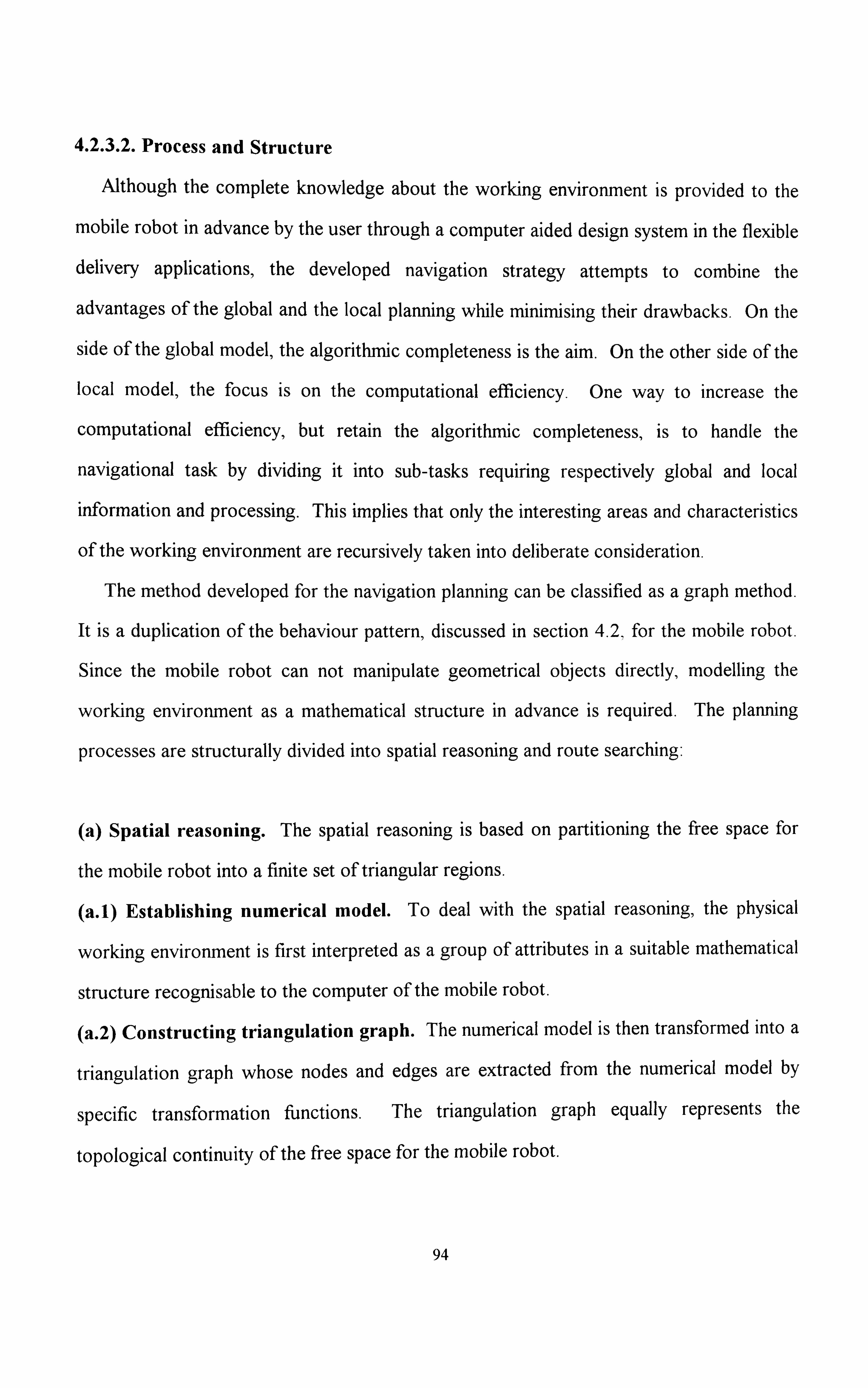
4.2.3.2. Process and Structure
Although the complete knowledge about the working environment is provided to the
mobile robot in advance by the user through a computer aided design system in the flexible
delivery applications, the developed navigation strategy attempts to combine the
advantages of the global and the local planning while nýiinimising their drawbacks. On the
side of the global model, the algorithmic completeness is the aim. On the other side of the
local model, the focus is on the computational efficiency. One way to increase the
computational efficiency, but retain the algorithmic completeness, is to handle the
navigational task by dividing it into sub-tasks requiring respectively global and local
information and processing. This implies that only the interesting areas and characteristics
of the working environment are recursively taken into deliberate consideration.
The method developed for the navigation planning can be classified as a graph method.
It is a duplication of the behaviour pattern, discussed in section 4.2, for the mobile robot.
Since the mobile robot can not manipulate geometrical objects directly, modelling the
working environment as a mathematical structure in advance is required. The planning
processes are structurally divided into spatial reasoning and route searching:
(a) Spatial reasoning. The spatial reasoning is based on partitioning the free space for
the mobile robot into a finite set of triangular regions.
(a. 1) Establishing numerical model. To deal with the spatial reasording, the physical
working environment is first interpreted as a group of attributes in a suitable mathematical
structure recognisable to the computer of the mobile robot.
(a. 2) Constructing triangulation graph. The numerical model is then transformed into a
triangulation graph whose nodes and edges are extracted from the numerical model by
specific transformation functions. The triangulation graph equally represents the
topological continuity of the free space for the mobile robot.
94

(b) Route searching. Once the triangulation graph has been constructed, the
corresponding nodes to the start and goal postures are identified. A graph-searching
algorithm is then implemented to find a solution path connecting the two nodes. (b. 1) Global journey searching. The solution path on the triangulation graph is called a journey. The produced journey is not yet a physical route for the mobile robot to directly
execute. It is only an isolated sub-set of the free space, representing a globally preferable
movement trend of the mobile robot towards the goal.
(b. 2. ) Local route rinding. Since the journey physically represents a sub-set of the free
space for the mobile robot, the final route to be executed is generated within the journey.
Due to the clearance space of the journey, alternative routes can be considered to handle
unexpected obstacles and uncertainties.
The route produced is finally interpreted as an associated operation scheme which
constitutes the performance of the mobile robot along the route. According to the
operation scheme, motion and perception commands will be derived and carried out at the
executing stage of the navigation strategy. Although the computational effort is huge
when planning navigation for the mobile robot in a large and complicated working
environment, the calculation is decreased by carefully and recursively identifying only the
parts of the working envirorument required for global or local considerations.
4.3. SPATIAL REASONING
The spatial reasoning approach adopts the triangulation algorithms
developed in chapter three. The configuration space of the mobile robot is identfied first,
and the physical obstruction mapped onto the configuration space to generate the
configuration obstacles. The configuration free space is then partitioned into a continuous
set of triangular regions. Specific functions are subsequently used to transform the
95

triangular regions into a triangulation graph. If the configuration free space of the mobile robot is connected, the triangulation graph is a connected graph. Finally, the start and goal postures of the mobile robot are retracted onto the triangulation graph according to the topological containment.
4.3.1. Establishim! Numerical Model
When establishing a numerical model, the configuration space formulation is applied. The configuration free space of the mobile robot is obtained by shrinking the mobile robot to a point, and expanding the physical obstacles accordingly. The navigation problem Is thus transformed to that of moving a point robot amongst the enlarged configuration
obstacles.
4.3.1.1. Configuration Space of Mobile robot
Six parameters are minimally required to define the status of a free-flying single rigid
object in a three-dimensional space; three for the position of a reference point on the
object, and three for the orientation with respect to axes passing through the reference
point. The mobile robot is a single rigid object with three identical wheels and a hard
suspension. Since it is constrained to move on the level ground of the manufacturing
environment, the vertical displacement to the ground surface is restricted. In addition, the
mobile mechanism can rotate about its centre axis, which is perpendicular to the ground
surface, and only one orientation is variable. That is, three constraint equations are
generated to reduce the number of the status parameters of the mobile robot from six to
three; two for position and one for orientation. The dimensions of the configuration space
of the mobile robot are three. This theoretically supports the transformation of the
navigation problem for the mobile robot to an equivalent geometrical problem for the
projected images, as described in section 4.2.1.1, by using the orthographic projection to
define the associated co-ordinate axes.
96

(a) Choosing reference. Due to the omni -directional mobility, the centre of MR is a
perfect candidate for the reference point. The three-dimensional configuration space of MR is illustrated in Fig. 4.3. A Cartesian co-ordinate frame Fw is embedded in the level
ground surface or the projection plane E. The origin and two axes are denoted by Ow,
Xw and Yw respectively. Another Cartesian co-ordinate frame Fm is attached to MR.
The origin of Frn, denoted by Orn, is superimposed on the centre of AIR, and the Xm axis is aligned with the heading direction of AIIR. Every point of MR has a pair of fixed co-
ordinate attributes with respect to Fm, and Fm is a co-ordinate frame moving within Fw.
A configuration of MR is hence a specification of Fm with respect to Fw.
(b) Configuration and posture. Since the centre of MR is identical with Om and the
angle between Xm and Xw at any instant is equal to the heading direction of AIR, a
configuration of MR can also be equally described by the quantity of the corresponding
posture of the mobile robot with respect to the working environment. For example,
posture I in Fig. 4.3(a) is represented as a triple (a, b, )(x) where a and b detertnine the
position of the centre of MR (origin Orn of Fin) with respect to Fw, and (x determines the
heading of MR (orientation of the Xm axis) with respect to the Xw axis. Posture I
corresponds to configuration I in Fig. 4.3(b).
Conf-iguration space. The configuration space of MR, denoted by C, is the union of
all possible configurations of MR. The construction of the configuration space C of AIR is
a continuous mapping from the projection plane E.
E->C- R2-->R 3
A point in E can be mapped onto a vertical line in C. As illustrated in Fig. 4.3(b), a three-
dimensional Euclidean frame Fc is embedded in the configuration space C, whose axes are
denoted by Xc, Yc and 0 respectively. Practically, Xw, Yw and Ow of frame Fw can be
97

treated as Xc, Yc and Oc of frame Fc directly, and the 0 axis as the axis normal to plane E and passing through Ow.
Yw
Yc
f
b
E posture 2 Ym
------------ --- Ym
I, O=P exrn
xm O=a
nj MR posture I
Fw Ow
(X
Oc, 0
ß
xw
(a) Orthographic projection Om overlaps with centre of MR Xm aligns with heading of MR
Xc
(b) Configuration space A patb by discrete navigation
Figure 4.3. Establishing configuration space
Since the mobile robot has an omni-directional mobility mechanism, whose driving and
steering motors are independently controlled to move forward and backward and revolve
at a place about the centre axis, all configurations (postures of MR) in C are valid if there
is no physical obstruction. The configuration space of MR is hence an open three-
dimensional space. In other words, every two configurations are continuous in C since the
two corresponding postures of MR can be connected by a route in E, although a discrete
navigation mode may be required. A path between configurations I and 2 in the
configuration space is illustrated in Fig. 4.3(b). The route on the ground surface E
between postures I and 2, as shown in Fig. 4.3(a), corresponds to the path, and the route
is performed by the discrete navigation:
turn(-a), move(e-a), turn(+90'), move(f-b), and turn(-90'+P).
6 4
f path
confi atioý
40 Orn
point robot /&onfiguration 2
98

4.3.1.2. Mapping Obstacles onto Configuration Space
Since the mobile robot navigation is physically constrained by objects in the
manufacturing environment, images WE and OBi's have to be mapped onto the
configuration space of MR. Let the sub-set of plane E occupied by MR at a configuration
c be represented by MR(c). The configuration obstacle COBi in space C associated with
an obstacle image OBi is a region defined by:
COBi=ýcc-C"R(c)r-)OBi#0j, COBi(--C, ic=[O, h].
The union of all configuration obstacles is called the configuration obstacle region-
hh U COBi =fce CVtIR(c)n U OBi: #O). i=O i=O
The configuration free space CF is the sub-set of C excluding the configuration obstacle
region:
CF=C- U COBi =ýce C"R(c)n U OBi =0). i=O i=O
Since MR is constrained to move within WE, CF should be revised to:
CF= ýc cz C[UR(c)(-- WE /\ MR(c)(-) U OBi =O ý- i=O
The configuration free space can also be produced by mapping the collision-free working
environment WEF onto the C space-
h
CF=jceC"R(c)(--TfEF, WEF=[fE-UOBi). i=l
A configuration in CF is a free configuration whose corresponding posture of the mobile
robot is collision free.
In practice, the mapping is performed by the following equations:
VP(EMR
Xw(p): --Xw(om)+(Xm(P)COSO-Ym(P)sinO)
Yw(P)=Yw(Om)+(Ym(P)sinO+Ym(P)COSO)
99

where P is a point of MR, 0 is the heading of MR with respect to Fw, (Xw(Om), Yw(Om))
is the co-ordinates of the centre of MR (origin of Fm) with respect to Fw, and
(Xw(P), Yw(P)) and (Xm(P), Ym(P)) represent the co-ordinates of point P with respect to
Fw and Fm respectively. The geometrical symmetry of the mobile robot is considered in
order to rapidly build the configuration free space for MR. Since MR is a circle and Om is
at the centre of MR. the cross section of a configuration obstacle COBi at a fixed
orientation 0 can be generated by enlarging the dimension of OBi with r units which is the
radius of the mobile robot. Constructing COBi is then accomplished by extending the
cross section vertically along axis E) subject to the imposed restriction on the heading of
the mobile robot. In the application, the [7c, -7c) interval of the steering angles is adopted.
The configuration obstacle COBi is hence a tower with 27u height in the three-dimensional
configuration space. Figure 4.4 illustrates an example configuration obstacle, and its
construction.
Yw
EI original OBi
y
Ym xm 0
JMR
Fw Ow
(a) Orthographic projection
xw
100

------------------- Yc (Yw)
Fc conliguration obstacle COBi
Oc (OW) x
(b) Enlarging dimension with r
Xc (Xc)
0
Om
yc Fc x
-lt -
(c) Extending vertically
Figure 4.4. Constructing configuration obstacle
4.3.1.3. Polygonal Approximation
It has been learned from section 4.3.1.2 that a convex vertex of an obstacle image
results in an arc surface when building the configuration obstacle for the mobile robot.
Since directly dealing with arc surfaces is difficult and computationally expensive, most
planning methods apply approximation approaches, such as [135], to the arc
interpretation. An approximation approach capable of generating prism configuration
obstacles is proposed to cut computational costs. The processes of the approach are
illustrated in Fig. 4.5 and outlined as follows:
y
I Fw Ow x
(a) Orthographic projection
r
---------- ----------------------- r
Yc OBi
r r ----------- ------------- r
/r
Om y -------
E)=o Fc w Xc
Oc
(b) Enlarge by radius r
101
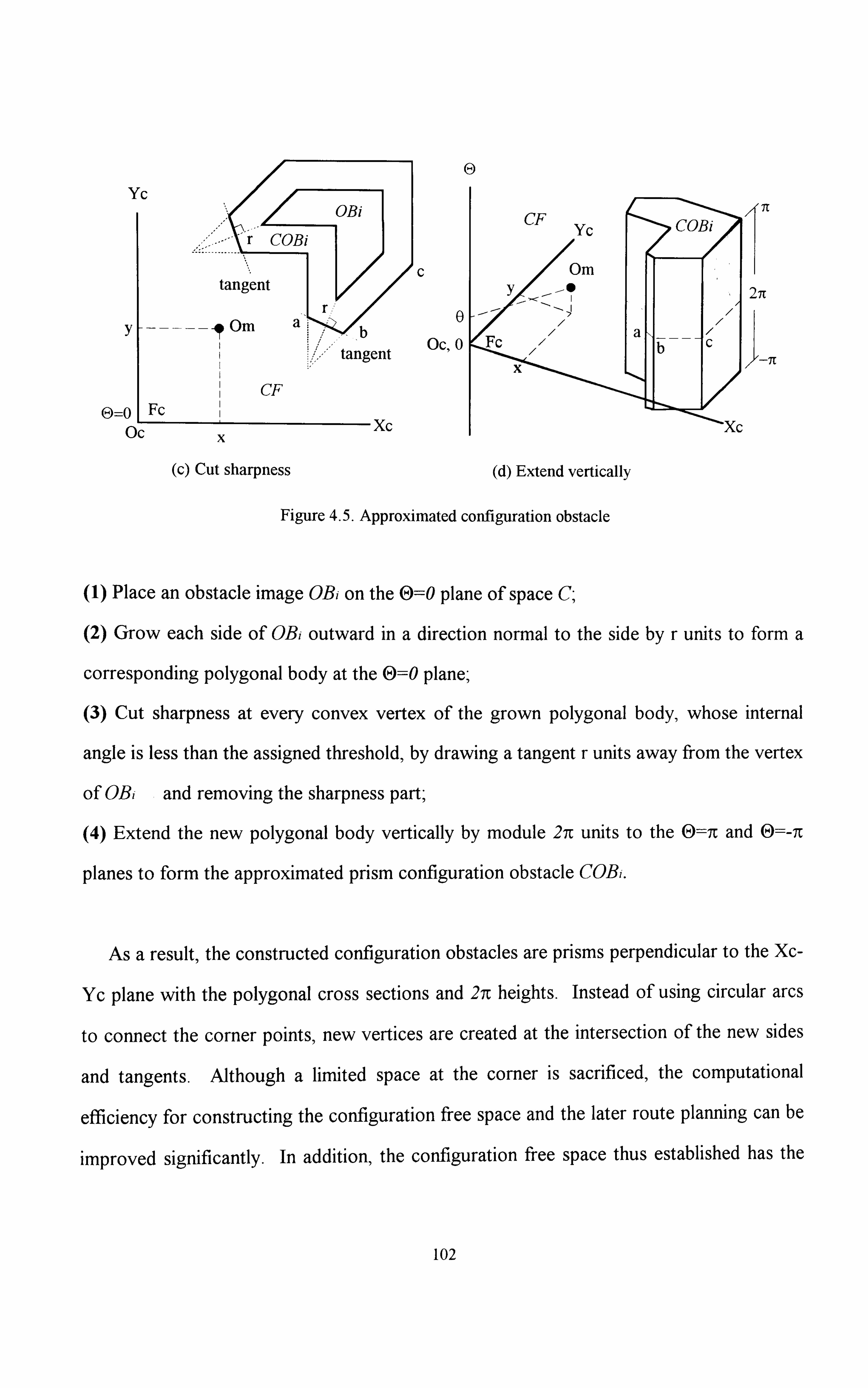
a
y
6=0 L Oc
Yc
------ Om
Fc
x
(c) Cut sharpness
c 0 b
ocý 0 tangent
- Xc
(d) Extend vertically
Figure 4.5. Approximated configuration obstacle
(1) Place an obstacle image OBi on the 0=0 plane of space C.
Y 271
/-71
(2) Grow each side of OR outward in a direction normal to the side by r units to form a
corresponding polygonal body at the 0=0 plane;
(3) Cut sharpness at every convex vertex of the grown polygonal body, whose internal
angle is less than the assigned threshold, by drawing a tangent r units away from the vertex
of OR and removing the sharpness part;
(4) Extend the new polygonal body vertically by module 27r units to the 0=7c and 0=-7r
planes to form the approximated prism configuration obstacle COR.
As a result, the constructed configuration obstacles are prisms perpendicular to the Xc-
Yc plane with the polygonal cross sections and 27c heights. Instead of using circular arcs
to connect the corner points, new vertices are created at the intersection of the new sides
and tangents. Although a limited space at the corner is sacrificed, the computational
efficiency for constructing the configuration free space and the later route planning can be
improved significantly. In addition, the configuration free space thus established has the
102

extra tolerance at the corner to account for the uncertainties of the mobile robot. The
space sacrificed by the approximation approach can be reduced by increasing the threshold
angle (90' at present) at step (3) and recursively performing step (3), but at the expense of the computational efficiency.
4.3.2. Constructing Triangulation Graph
The configuration space formulation is a mathematical representational tool to describe
the states of the mobile robot in the environment. Once the mathematical model has been
established, computational algorithms can be implemented on it to plan the navigation. The developed navigation strategy treats the mathematical representation as a graph, and
searches on the graph to produce a journey for the mobile robot. To construct the graph,
transforming the configuration space C into the attributes of the graph is necessary.
4.3.2.1. Triangulating Configuration Free Space
The graph transformation is based on decomposing the configuration free space of the
mobile robot. Since the configuration obstacles established in space C are prisms
perpendicular to the Xc-Yc plane, with approximate polygonal cross sections and 271
heights, the orthographic projection of the configuration free space CF onto the Xc-Yc
plane is a polygonal region containing polygonal holes. Using the triangulation algorithms
developed in chapter three, the orthographic projection of CF can be triangulated into a
finite set of non-overlapping triangular regions-
(1) Equivalent simple polygon. The bridge-building operation is performed first to
transform the orthographic projection of CF into an equivalent polygonal region.
(2) Triangulation. Once the equivalent polygonal region has been produced, it can be
triangulated into a set of triangular regions.
Although the triangulation is performed on the orthographic projection of CF, each
triangular region actually represents a prism , in the C space, normal to the Xc-Yc plane
103

and with a triangular cross section and 271 height. CF is thus decomposed into a collection
of non-overlapping triangular prismatic spaces whose union is CF. This triangulation of CF is subsequently used as the spatial features of the configuration free space to form a
graph, which is called the triangulation graph.
4.3.2.2. Triangulation Graph
To produce the nodes and edges of the triangulation graph Gy--(NTET) from the
triangulated CF, an implicit way of topological modelling is applied-
(a) Node. Modelling the node set NT is done by extracting some distinctive spatial features of the triangulated configuration free space; each triangular prismatic space being
abstractly interpreted as a node. The configuration free space is then represented by a set
of nodes.
(b) Edge. The edge set ETis a binary relation on NT, which consists of unordered pairs of
nodes. A pair of nodes whose representing triangular prismatic spaces are spatially
adjacent are connected by a non-directed edge. Two triangular prismatic spaces are
spatially adjacent if they share a common facet. The graph is accomplished by connecting
edges in the node set, NT.
The configuration free space of the mobile robot is finally modelled as a non-directed
triangulation graph, associated with the triangulation of the orthographic projection of
CF. Obviously, the triangulation graph being connected implies that the configuration free
space is connected. Since the triangular prismatic spaces are convex, it is easy to find a
free path connecting any two configurations in the same triangular prismatic space. That
is, all configurations within a triangular prismatic space are qualitatively equivalent. For
two configurations, each belonging to one of a pair of adjacent triangular prismatic spaces,
104

it is also easy to compute a free path connecting them by crossing the facet shared by the
two adjacent spaces. In addition, due to the geometrical simplicity of the triangular
prismatic spaces, the adjacency of any two triangular prismatic spaces is easy to examine,
and the degree of every node of the non-directed triangulation graph is at most three.
Theorem 4.1. Given a collision-free working envirorunent REF with n vertices in total,
the triangulation graph constructed is GT--(NTET). The node and edge sets of GT, denoted
by INTI and JETI , are both of order O(n).
Proof: Since TfEF has n vertices, WEF has k concave (km) and n-k convex vertices. At most the cut-sharpness is performed k times by the approach in section 4.3.1.3. Each operation produces two new vertices to replace the original one. The orthographic projection of the configuration free space CF thus produced is a polygonal region with polygonal holes, which has at most n+k vertices in total. Since n:! m+k:! ý2n, n+keO(n). Triangulating the n+k-vertex polygonal region with polygonal holes thus generates O(n) triangular regions and O(n) triangulating diagonals according to Theorem 3.10 of chapter three. Every triangulating region is represented by a node in NT, and every triangulating diagonal corresponds to an edge in ET. Therefore, INTI and JETI are both of order O(n).
The proof is completed. El
As a result, the numbers of the nodes and edges of the triangulation graph are of the
same order of complexity, and both are linearm the number of the vertices of WEE
Figure 4.6 illustrates the processes of the implicit topological modelling and
triangulation graph correspondingly constructed.
105

WEF BO
OBI
Ym
OB2
--I A/M
:1
Yw OBO
E Xw
Figure 4.6(a) Orthographic projection of manufacturing environment
- ------------------------------ -- ---------- - -------- (70BO
-------------------------- ------------------------------ - -------------------- ---------------------- CF
----------
---------------- COB] Ym xm
(Yw) Yc IC
-------------- COB2
Ll
C ---- 0 ---
B
----------
- ------------------- --------------- - ------- ---------- --------- ------- -------------------------
0 %ý- xc (xw) [7E, -7E]
Figure 4.6(b) Orthographic projection of configuration space n=29, h=2
106

(YW) Yc
0 LC
17T, -7T]
-------- -- 1411i 3 CF
3 /7 8
COB] 2 30
ý% 25 /24
/29 6\\// --
22 2 COB2 \27
19 16ý 28\ COBO lira -------- 17
- Xc (Xw)
Figure 4.6(c) Triangulation of configuration free space triangular regions: n+2h-2 triangulating diagonals: n+3h-3
Om
Figure 4.6(d) Associated triangulation graph
The produced triangulation graph GT physically stands for the adjacent relationship
among the triangular prismatic spaces resulted from the triangulation of CF. In other
words, GT consists of an implicit network of one-dimensional edges, reflecting the
topological connectivity of the configuration free space. The edges could also be
explicitly obtained by selecting a representative point (configuration) for every triangular
prismatic space, and joining a physical path between the representative points of every pair
of adjacent triangular prismatic spaces. However, the explicit triangulation graph is
restrictive since it does not provide the useful information about the clearance space, and
107

alternative paths, for the mobile robot to deal with the kinematics/dynamics constraints and unexpected obstruction at the executing stage. The implicit triangulation graph is flexible, and the journey searching operation on it will be discussed next.
4.4. SEARCHING FOR GLOBAL JOURNEY By transforming the configuration free space CF of the mobile robot to a non-directed
triangulation graph GT--(NTET), the navigation planning has proceeded from finding a free
path in the configuration space C to finding a path in CF, and finally to searching for a
graph path on GT. Well developed graph searching algorithms can be applied to the
triangulation graph to generate a solution graph path connecting the nodes corresponding
to the start and goal configurations (postures) of MR. To search for a solution graph path
on the triangulation graph, the start and goal configurations of MR have to be retracted to
the triangulation graph first. A weight function has to be defined to evaluate the weight of
every node and edge of GT SO that the graph searching algorithms can be implemented to
work on GT. The solution graph path generated is called a journey, physically representing
a globally preferable movement trend of the mobile robot towards the goal. A free path in
C is finally produced in the journey, consisting of a series of local routes and the
associated operation schemes.
4.4.1. Retraction bv Point Containment
In the triangulation graph GT--(NTET), a node of NT represents a collection of free
configurations ofMR in C, enclosed by the triangular prismatic space corresponding to the
node. All configurations within the triangular prismatic space are qualitatively equivalent,
and the corresponding collision-free postures of the mobile robot are also represented by
the node. Retracting the start configuration (posture) S and goal configuration (posture)
G to graph GT IS, therefore, equivalent to finding the nodes of GTwhose representing
108

triangular prismatic spaces contain S and G. Such a problem can be solved by performing the point containment test on the orthographic projection of the triangulated configuration free space.
Given a test point and polygon in a plane, the point containment test is to determine
whether the point is inside or outside the polygon [134]. In the application, the polygon to be tested is a triangular region. A point P is inside or on the boundary of a triangular
region ARK, PcAIJK, if and only if
A(AIJK)=A(AIJP)+A(AIPK)+A(ApjK).
Point P is outside ARK, POARK, if and only if
A(AIJK)<A(AIJP)+A(AIPK)+A(ApjK).
In the equations, A(AJJK) is the area of ARK, computed by:
1 X(I) Y(I) 1
A (A IJK) abs( X(ý Yo 1 X(K) Y(K) 1
where X(J) and Y(J) are the co-ordinates of point I with respect to the Euclidean frame
embedded in the plane.
By comparing the projection images of configurations S and G, on the Xc-Yc plane of
the C space, with that of each of the triangular prismatic spaces, the triangular prismatic
spaces containing S and G can be identified. The representing nodes are subsequently the
start and goal nodes on the triangulation graph, denoted by Ns and Ng respectively.
4.4.2. Optimal Global Journey
Once the spatial reasoning has been completed, the implicit triangulation graph can be
manipulated to search for the optimal solution graph path. The solution graph path
generated is an ordered sequence of nodes and edges beginning from Ns, and terminating
at Ng. Since the nodes represent a set of triangular prismatic spaces in CF, and the edges
109

represent the adjacency of these triangular prismatic spaces, the solution graph path
spatially describes a channel of configuration free spaces containing the start and goal
configurations. No explicitly physical route is planned directly from the triangulation
graph, instead a global journey representing a connected subset of CF. The final collision-
free navigation of the mobile robot, from postures S to G, can be planned in the global
journey as a path in the channel of configuration free space. To use graph searching
algorithms, a weight function has to be defined to evaluate the triangulation graph.
4.4.2.1. Weighted Triangulation Graph
A weighted triangulation graph GT--(NTET) is a graph .. every edge has an Onwicir-K
associated weight, typically given by a weight function W. ET-->R mapping the edges to
real-valued weights: W(Ni, N2) if Ni, N2eNTand Ej, 2::: --(Ni, N2)cET
ýO otherwise
The weight of a graph path PG: --(No, Nj,..., Nk) is the sum of the weights of its constituent
edges- k
W(PG)-= i=l
W(Ni -1 A), where Ni eNTand (Ni-i, Ni)c=ETf6r i=l to k.
The optimal weight from Ni to N2is defined by (min I W(PG): Ni-PG->N21 if there is a graph path PG from Nj to N2
6(Ni, N2)--ý
ýoc otherwise
A graph path with the optimal weight is the shortest graph path. The shortest graph path
from the start node Ns to goal node Ng in the weighted triangulation graph is hence defined
as a graph path PG whose weight is optimal:
W(P G): -- 6 (Ns, Ng).
110

Obviously, there is no loop in the shortest graph path PG from Ns to Ng, PG=(N,,..., Ng),
otherwise, the generated optimal weight from Ns to Ng is not the optimal, and can be
further reduced:
N,, NjEz- (Ns, -- -Ng I => Ni#Nj
Although the shortest graph path generated on the weighted triangulation graph is not the
route to be directly executed by the mobile robot, it is still useful to have the optimal
weight indicating the minimum costs for reference, that may be expected at the executing time. To determine the weight function for an edge between two adjacent nodes for this
purpose, the physical contents of the edges have to be defined. In other words, the
motion principles concerning how the mobile robot performs the navigation from one
triangular prismatic space to an adjacent one should be realised.
4.4.2.2. Motion Principles
As described in chapter two, the mobile robot has a mechanism which can move
forward and backward, and revolve at a place about the centre axis, and supports two
navigation modes; continuous and discrete. In terms of realising the physical contents of
the edges of the triangulation graph in order to define the weight function, the discrete
navigation mode provides a better reference indication of costs, and is more essential, than
the continuous mode.
In the discrete navigation mode, the moving and steering motions of the mobile robot
are performed at different time intervals. That is, the translation distance and the angular
displacement of MR between two configurations (postures) are considered independently.
There is no change in the heading direction of the mobile robot while the translation motor
is working:
d0 =O
dD 0 :;, --0 .,. w= =O or
dD dt dt
III

moving straight . -. dYc=dYw
=tano=constant .,. d(tanO).
0 ... (O=C/O==O. dXc dXw dt dt '
and vice versa, v-- dD=:
O while the rotation motor is workin ; where dt 91)
(dD)2=[(tAC)2+(ayC)2]=[(aXW)2+(ayW)2].
Figure 4.7 illustrates the motion schedule of the discrete navigation in Fig. 4.3, where the
total performing time of the navigational task is divided into a series of time intervals.
Rotation displacement 0 +90 0 -90+0 Translation distance 0 e-a 0 f-b 0
beginning ti Q0 t4 terminati. c rý (performing time)
Figure 4.7 Motion schedule of discrete navigation
Apart from the motion principles concerning the movement of MR using the discrete
navigation mode, no slippage is assumed in the application. The kinematics constraint
defining the no-slippage condition is
(dXw)Sino-(dy, w)coso=o.
Since dYw--vSinO=dYc and dXw--vCOSO=dXc, (dXc)SinO-(dYc)COSO=O.
In the above equations, v and co are the instantaneous translation velocity and orientation
velocity of the mobile robot respectively, t is the time, and all the other terms are subject
to Fig. 4.3.
As a result, there are only horizontal and vertical movements while the point robot is
moving in the configuration space by the discrete navigation mode. To resolve a path,
produced in the configuration space, into a route and associated operation scheme, the
horizontal parts of the path constitute the route, and the vertical parts the associated
operation scheme. In other words, the route describing the trajectory of the centre of MR
in WE consists of a sequence of straight-line segments in the E plane. The associated
112

operation scheme' a continuous sequence of orientatIons of MR along the route,
which are constant along a straight-line segment, and change only at the intersection of two consecutive straight-line segments.
4.4.2.3. Graph Searching Algorithm
Before the weight function is defined, graph searching algorithms are discussed in
order to realise how the weight function is applied in the algorithms. Given the weighted
triangulation graph evaluated by the defined weight function, the graph searching
algorithms are implemented on it to search for the optimal graph path. The graph
searching algorithms can be outlined as follows-
(1) Put start node Ns on a list called OPEN and compute f (Ns)
(2) If OPEN is empty, exit with failure; otherwise continue.
(3) Remove from OPEN the node whose f value is the smallest and put it on a list called
CLOSED. Call this node Ni. (Resolve ties for minimal f values arbitrarily, but always in
favour of the goal node).
(4) If Ni is the goal node Ng, exit with the solution graph path obtained by tracing back
through the pointers; if Ni is on CLOSED, go to (2); otherwise continue.
(5) Expand node Ni by finding all of its successors. [If there are no successors, go
immediately to (2). ] For each successor Ni, compute f(Ni) by f (Nj)=f(N, )+W(N,, Nj). Put
these successors on OPEN, associating with them the f values just computed, and provide
pointers back to Ni.
(6) Go to (2).
In the steps outlined, the OPEN list contains a set of nodes to be The set of
nodes and pointers, generated by the algorithms, forms a tree (the search tree) with the
nodes on OPEN at the tips of the tree. The weight function W(N,, Nj) is used to define
113

the required cost from nodes Ni to Nj along the edge (N,, Nj). Providing that the cost to
achieve a node N, is f(N), the cost to achieve its successor node Ni through the edge (N,, Nj) is f (N) plus W(N,, Nj), and denoted by f(Ni). The CLOSED list maintains a set of nodes whose final optimal weights from Ns have already been determined.
The Dijkstra algorithm [121][122] is a typical example of such a graph searching
algorithm. The running time for the Dijkstra algorithm is O(IV12+IEI) provided that the
input graph has IVI nodes and JEJ edges, and can be modified to 0((IVI+IEI)IgIVI) [83].
Another example is the A* algorithm [121] which uses o- heuristic function to improve
the computational efficiency. It works by replacing the f function, f(Nj)=f(N, )+W(N,, Nj)
at step (5), with a new one, f(Nj)=g(Nj)+h(Nj, Ng). In the new f function, g(Nj) is the
actual cost from Ns to Ni produced by adding the weight W(Ni, Ni) to the actual cost from
Ns to Ni, denoted by g(N), and g(Nj)=g(N, )+W(N,, Nj). h(Nj, Ng) is the heuristic function
indicating an approximated cost from Nj to Ng. It has been theoretically shown that the A*
algorithm is efficient as long as the heuristic function is a lower bound of the actual cost
[ 12 1 ]. The A* algorithm becomes an ordinary one if the heuristic function is assigned to
be zero. - aThe Euclidean distance is usually used to define the heuristic function
in the navigation planning.
4.4.2.4. Weight Function
Two free configurations are connected if and only if they are linked by a free path. In
the configuration space C ofMR, a free path between two connected free configurations S
and G is a continuous map Pc: [0,1]->CF, CF is the configuration free space with
Pc(O)=S and Pc(])=G. Since Pc is produced using the discrete navigation mode, Pc
should consist of a sequence of horizontal straight-line segments at different E) planes of
space C, and vertical straight-line segments connecting the horizontal segments. The final
local route on plane E and the associated operation scheme, to be performed by MR (the
mobile robot) at the executing stage, are then mapped from Pc. Obviously, the mapping
114

can be accomplished by using the orthographic projection of Pc onto plane E to produce the route. That is, the route is the projection image of Pc on E, which should be
polygonal and zigzag shaped. In addition, the angle between two consecutive segments of the zigzag shaped route should be equal to the quantity of the corresponding vertical
segment of Pc. The operation scheme is consequently produced. Figure 4.8 is an illustration.
S3 space path Yc
route
xc ------ --------
triangular prismatic space
Figure 4.8 Space path vs. route and associated operation scheme
As already discussed, the path Pc between S and G is planned in the optimal
journey, and the optimal journey is generated by searching on the triangulation graph
according to the weight function defined. Since the optimal journey is a channel of
configuration free space consisting of triangular prismatic spaces, one way to plan Pc in
the spatial channel is to select representative configurations for the constituent triangular
prismatic spaces, and to link every pair of adjacent configurations by a free path. Two
configurations are adjacent if their representing triangular prismatic spaces are identical or
adjacent. Once the selection is defined, the movement of the point robot from one node N,
to another Nj on the triangulation graph along the edge (N,, Nj) is simply interpreted as the
path linking the representative configurations for the adjacent triangular prismatic spaces.
The weight WWAD of an edge (N,, Nj) can thus be defined to be the cost of the path
115

between the representative configurations. As a result, the definition of the weight function is highly related to the selection of the representative configurations for the
triangular prismatic spaces.
The cost of a path can be interpreted as metrics in many forms, which is often used to
represent time, distance, turn, energy, penalties, loss, or any other quantity that
accumulate linearly along a navigation (space path) that one wishes to minimise. In the
discrete navigation mode, a path in C is composed of a sequence of horizontal and vertical
straight-line segments. A horizontal segment is a translation distance to be performed by
the translation motor, and a vertical segment is an angular displacement to be carried out
by the rotation motor. Since a path with short translation distances and few angular
displacements is preferred, and the translation distance and angular displacement have
different units, the time consumed is used to express the cost. The weight function can be
derived consequently. If the maximum safe translation velocity and rotation velocity for
the mobile robot are given, the time to navigate from one configuration to
another is hence lower-bounded by:
time--Y translation distance rotation displacement
translation velocit y rotation velocity
As to the selection of the representative configurations for the triangular prismatic spaces,
the central vertical segment of the facet shared by two spaces is selected to represent the
triangular prismatic space to enter. It will be further discussed in section 4.5.
A weight function W(N,, Nj) has been defined to express the time cost required from
nodes N, to Nj along edge (N,, Nj). The cost to achieve a node Nj, f(NI), is equal to
W(N,, Nj) plus the cost required to achieve node Ni, if Ni is an ancestor of Nj and they are
connected by edge (N,, Nj). As in Fig. 4.8, the start configuration S is given by a triple
(XS, YS, OS), and the representative configuration of node Nj which contains S is a triple
(XI, YI, 01). Since Ns=Ni, (XI, YI, 01)=(XS, YS, OS) and f(Ns)=f(Nj)=O;
f(N2)=f(Nj)+W(Ni, N2), where
116

W(Nj, N2)-= 02-01
+ ý(-X2-Xlý+(Y2-Ylý
and 02=tan-'( Y2-YI CO safe Vsafe X2-XI '
W(N2, N3): -- 03-02
(0 safe
f(N3)=f(N2)+W(N2, N3), where
(X3-X2)2 +(Y3-Y2)2 and 03=tan-' Y3 - Y2
Vsafe X3 - X2
Similarly, the cost to achieve a node is thus evaluated. Although the shortest graph path is
just the optimal journey, and is not the route to be executed by the mobile robot, the
optimal weight still indicates the performing time for reference, which is a lower bound of
what may occur at the executing time if no unexpected obstruction is encountered.
4.4.2.5. Clearance of Solution Channel
The shortest graph path generated on the explicit triangulation graph is physically a
spatial channel. This spatial channel represents a connected subset of the configuration
free space containing the navigation solutions for the mobile robot from S to G.
Navigation along the graph path physically means that the mobile robot begins its journey
from the start triangular prismatic space, passes consecutively through all constituent
triangular prismatic spaces of the graph path, and terminates at the goal triangular
prismatic space. Since every configuration in CF corresponds to a collision-free posture
of MR in WK) a path produced in the spatial channel can always be mapped to a collision-
free navigation for the mobile robot to perform in the manufacturing environment.
The final route and associated operation scheme applicable to the mobile robot will be
planned inside the spatial channel according to the motion principles of the discrete
navigation mode. Obviously, when the mobile robot performs a path thus produced in the
optimal channel, some clearance to the obstacles can be assured. Due to the clearance, the
continuous navigation mode consisting of curve routes can also be planned in the spatial
channel.
117

4.5. FINDING LOCAL ROUTE AND OPERATION SCHEME Once a solution graph path (the optimal journey) from the start to the goal node has
been generated on the triangulation graph, a channel of configuration free space contalning
configurations S and G can be identified. The next task Is to locally produce a feasible
path connecting S and G in the spatial channel. This path can then be used to derive the
route and associated operation scheme for the mobile robot. In addition, the function is
developed of proposing alternative paths for the mobile robot to handle accidental happenings, such as avoiding collisions with unexpected obstacles.
4.5.1. Normal Case Usim! Central Line
Since the triangulation graph only represents the topological connectivity of the
configuration free space, the generated graph path from the start to the goal node implicitly represents a channel of configuration free space, if such a graph path exists.
This solution spatial channel not only contains configurations S and G but also provides
vox'%vtx-5 possibilities of linking S and G within it. However, a qualified free path, consisting
of an ordered continuous combination of configurations from S to G within the channel,
should satisfy the physical constraints on the mobility mechanism of the mobile robot.
This ordered continuous combination of configurations from S to G should, in addition,
satisfy the navigation mode and cost requirements.
The motion principles concerning the physical constraints on the mobility mechanism
have been described in section 4.4.2.2, and the discrete navigation mode is used to
produce a solution free path. As a result, the solution free path must consist of a sequence
of horizontal straight-line segments at different E) planes of the C space, and vertical
straight-line segments connecting the horizontal segments. Also, the final local route and
associated operation scheme, for the mobile robot to perform in the manufacturing
118

environment, can be produced from the orthographic projection image of the solution free
path on plane E.
As to the cost requirements, a solution free path having a short travelling distance and few turns is preferred. Any path containing loops and identical configurations (position
and orientation) should not be considered, and the mobile robot should not go to a posture
more than once. Above all, the safety cost is the most important issue In the
application. One easy way to take safety into account is to plan a free path with tolerance for errors and inaccuracies. This tolerance can be realised by keeping some relatively large clearance between the mobile robot and the obstacles, and making the best use of the
on-board sensors, the impact of the uncertainties being relieved by the clearance, and
corrected by the sensors.
To plan a path, the fact that the spatial channel is composed of a sequence of
connected non-overlapping triangular prismatic spaces is considered. The central vertical
segment of the facet interfaced between each pair of consecutive triangular prismatic
spaces is used. The solution free path planned is the one that enables the point robot to
start from S, move upwards or downwards vertically to a suitable 0 plane, and move in
the 0 plane towards the first central vertical segment in order to leave the first triangular
prismatic space and enter the second. At the first central vertical segment, the point robot
moves upwards or downwards vertically again, subject to the other central vertical
segment of the facet interfaced between the second and third triangular prismatic spaces.
These movements proceed sequentially until the point robot arrives at the last triangular
prismatic space via the last central vertical segment. The point robot finally moves
horizontally towards the configuration whose position components are equal to those of
the goal configuration, and vertically to stop at
Once the polygonal free path is produced, the route and associated operation scheme
can be derived, by finding the orthographic projection image of the solution free path on
plane E, or the Xw-Yw plane. The route is polygonal and zigzag shaped, consisting of
119

straight-line segments on plane E. The operation scheme along a straight-line segment of
the route is constant, and equal to the angle of the straight-line segment with respect to
the Xw axis. The operation scheme at an end point of a straight-line segment is in a
transient state, the mobile robot changing its heading direction but not location. The sub-
routine program is outlined as follows-
Finding route and operation scheme in spatial channel without unexpected obstruction Sub-routine(Normal case) CurrentC. <-S- Position(CurrentC)ý<--Position(S). Orientation(CurrentC)<--Orientation(S) Ratio<---O. 5 DO
IF NextFacet(CurrentC)=O THEN Position(NextC)<--Position(G) ELSE Position(NextC)<-Position(VerticalSegment(Ratio, NextFacet(CurrentC))) END IF Orientation(NextC)4---Angle(Segment(Position(CurrentC),
)Position(NextC)), XwAxis)
NextCý(-(Position(NextC), Orientation(NextC)) OperationScheme<-Orientation(NextC)-Orientation(Currentc) Route<- Segment(Position(CurrentC), Position(NextC)) CurrentC<-NextC IF Position(CurrentC)=Position(G) THEN Operation S cheme=Orientati on(G)-Ori entation(CurrentC) STOP END IEF
LOOP
Figure 4.9 illustrates a route and associateAoperation scheme found within the solution
spatial channel. The clearance requirement is assured since the solution free path always
keeps some distance from the boundary facets of the spatial channel (configuration
obstacles). In addition, the route and operation scheme derived are specially suitable for
the on-board ultrasonic sensors to attain reliable information, since the horizontal parts of
the solution free path are always parallel with the boundary facets of the spatial channel.
120

Yw
xw triangulation navigation route
Figure 4.9 Projection image of solution channel Local route and operation scheme
4.5.2. Handling Unexpected Obstruction
The central-line free path produced is a good safe solution, since the clearance
provides the mobile robot with tolerance for control, model and sensing uncertainties.
Also, the path supports the best use of the equipped ultrason-ic sensors to perceive reliable
feedback. However, when an unexpected obstruction, which interferes with the original
global/local plan,, is encountered, handling behaviours must be activated. These
behaviours should propose alternative solutions, around the unexpected obstruction, to
achieve the goal, and help build a reliable mobile robot planner.
4.5.2.1. Type of Unexpected Obstruction
As described in section 4.2.2, an unexpected obstruction is likely to cause problems at
four levels of seriousness. In practice, the problems can also be classified into software,
hardware and external state failures [ 13 6] -
(1) Software failures are used to indicate logic errors and bugs in the programs. It is
assumed that the developed programs are logically correct, and the unexpected
obstruction is only due to hardware or external state failure.
(2) Hardware failures include physical errors and system inaccuracies of the mobile robot,
such as motor disability. It might not be possible to recover from a hardware failure.
121

However , it is reasonable to assume that a hardware failure of the mobile robot, in a
manufacturing application, is detectable and correctable, and the mobile robot is able to
continue functioning.
(3) External state failures describes the circumstance where the state of the world,
assumed by the mobile robot, does not match that perceived by the equipped sensors. Although an external state failure is sometimes interrelated with hardware failures in
practice, it is only used here to indicate an unexpected obstruction exclusive of the effects
caused by hardware failures.
At the planning stage of the navigation strategy, the mobile robot only deals with
unexpected *Wades classified as external state failures, and leaves hardware failures to
be handled at the executing stage. The handling behaviours for an unexpected obstacle are
hierarchically organised at the planning stage. The presence of an unexpected obstacle in
the path of the mobile robot need not immediately invoke the planner to produce a new
path to avoid the obstruction. Instead, the mobile robot waits in case the unexpected
obstacle will be cleared. If this simple handling behaviour fails, the unexpected
obstruction is propagated to a higher level of the handling behaviours. The handling
behaviours developed are classified into local detouring and global re-planning.
4.5.2.2. Detouring
When the simple wait-and-see handling behaviour fails, the control is propagated to a
higher level of the handling behaviours. At this level, the handler deals with the
obstruction if the presence of the unexpected obstacle does not disconnect the planned
spatial channel. The detouring handler is initiated to avoid the unexpected obstacle, by
locally adjusting the original path in the spatial channel. Handling the unexpected obstacle
at this level heavily relies on the perceiving ability of the mobile robot. Therefore, it Is
assumed that the equipped sensors are capable of reliably detecting or localising the
122
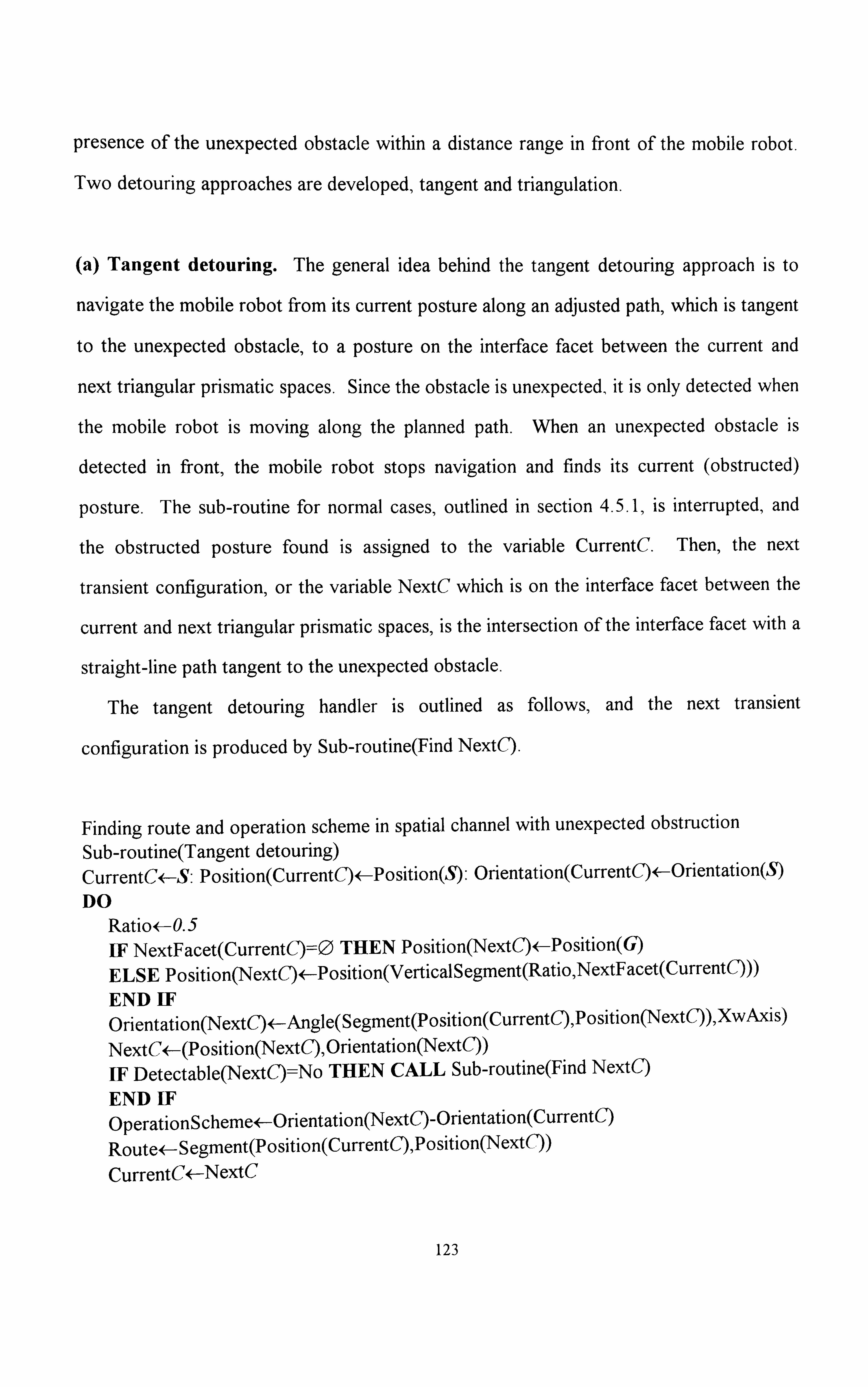
presence of the unexpected obstacle within a distance range in front of the mobile robot.
Two detouring approaches are developed, tangent and triangulation.
(a) Tangent detouring. The general idea behind the tangent detouring approach is to
navigate the mobile robot from its current posture along an adjusted path, which is tangent
to the unexpected obstacle, to a posture on the interface facet between the current and
next triangular prismatic spaces. Since the obstacle is unexpected, it is only detected when
the mobile robot is moving along the planned path. When an unexpected obstacle is
detected in front, the mobile robot stops navigation and finds its current (obstructed)
posture. The sub-routine for normal cases, outlined in section 4.5.1, is interrupted, and
the obstructed posture found is assigned to the variable CurrentC. Then, the next
transient configuration, or the variable NextC which is on the interface facet between the
current and next triangular prismatic spaces, is the intersection of the interface facet with a
straight-line path tangent to the unexpected obstacle.
The tangent detouring handler is outlined as follows, and the next transient
configuration is produced by Sub-routine(Find NextC).
Finding route and operation scheme in spatial channel with unexpected obstruction Sub-routine(Tangent detouring) CurrentC<-S- Position(CurrentC)<-Position(S). Orientation(CurrentC)<-Orientation(S) DO
Ratio<-0.5 ILF NextFacet(CurrentC)=O THEN Position(NextC)<-Position(G) ELSE Position(NextC)<-Position(VerticalSegment(Ratio, NextFacet(Currentc)))
END IF Orientation(NextC)<-Angle(Segment(Position(CurrentC), Position(NextC)), XwAxis)
NextC+-(Position(NextC), Orientation(NextC)) IF Detectable(NextC)=No THEN CALL Sub-routine(Find NextC)
END IF Operation S cheme+-Orientation(NextC)-Orientation(CurrentC) Route<- Segment(Position(CurrentC), Position(Next(. ))
CurrentC<-NextC
123

IF Position(CurrentC)=Position(G) THEN Operation S cheme=Orientation(G)-Orientation(CurrentC) STOP END IF
LOOP
Sub-routine(Find NextC) NextC'<-Line(Position(CurrentC), Position(Tangentpoint(Obstacle)))r-) NextFacet(CurrentC) Position(NextO<-Position(NextC') Orientation(NextC)<--Angle(Segment(Position(CurrentC), Position(Nextc)), XwAxis) RETURN
A tangent free path to avoid the unexpected obstacle is planned, and the physical
contact between the mobile robot and the unexpected obstacle is minimised to be at the
tangent point. Once the obstruction has been handled, the normal movement pattern
(central line) is called again to restore the navigation in the spatial channel. Figure 4.10
illustrates an example.
v
YW
L xw Figure 4.10 Tangent detouring
The tangent detouring handler locally proposes an adjusted path for the mobile robot
to avoid the unexpected obstacle. This adjusted path is tangent to the unexpected obstacle
and through the clearance space of the spatial channel. In general, there are two such
tangent detouring paths for the unexpected obstacle, and the one with the shorter distance
124
normal pattern from Fig. 4.9 tangent detouring

is used. Since only information about the width of the unexpected obstacle is required, the
tangent detouring approach is not computationally expensive. However, completeness is
not assured.
(b) Triangulation detouring. The second detouring approach uses operations similar to
the triangulation global planning approach, but in the local environment. It is based on
further decomposing the free space of the obstructed (occupied) triangular prismatic
spaces of the spatial channel into a set of smaller triangular prismatic spaces. A local
triangulation graph can be formed consequently. Searching for the optimal graph path on
this local triangulation graph generates a sub-local spatial channel within the obstructed
triangular prismatic spaces. A detouring route and associated operation scheme avoiding
the unexpected obstacle can be produced within the sub-local spatial channel, using the
central-line method described in section 4.5.1. If the unexpected obstacle does not
disconnect the spatial channel, the triangulation detouring approach is able to complete the
handling task by finding a sub-local free path, to avoid the unexpected obstacle, through
the clearance space of the spatial channel. The adjusted free path thus produced, or the
route and associated operation scheme found, is illustrated in Fig. 4.11.
Yw
L xw
G
normal pattern from Fig. 4.9 triangulation detouring triangulation from Fig. 4.9
---- ------- additional triangulation
Figure 4.11 Triangulation detouring
125

The triangulation detouring approach is specially suitable for dealing with cases when the unexpected obstacle can be precisely detected. Completeness of handling the
unexpected obstacle is assured, provided that the presence of the unexpected obstacle does not disconnect the spatial channel. Once the adjusted polygonal free path is
produced, the route and associated operation scheme to avoid the unexpected obstacle can be generated consequently by mapping the orthographic projection image of the produced detouring path onto the E plane. However, the triangulation detouring approach is more
expensive than the tangent detouring approach. Also, complete information about
geometrical features of the unexpected obstacle is required.
Two detouring approaches to locally modify the original path, planned in the spatial
channel, are developed to handle unexpected obstacles. When an unexpected obstacle is
detected, and Sub-routine(Find NextC) of the tangent detouring approach can not produce
a value for NextC, the triangulation detouring approach is initiated. Since handling
unexpected obstacles by the detouring approaches requires the obstacle information be
available at the handling instant, it is assumed that the equipped sensors are able to reliably
detect and identify the presence and geometry of the unexpected obstacle within a distance
range in front of the mobile robot. If this is not the case or the presence of the unexpected
obstacle disconnects the spatial channel, the obstruction will be propagated to the highest
level of the handling behaviours, described in the next section.
4.5.2.3. Updating Triangulation Graph and Re-planning
If a free path can not be produced in the spatial channel to locally avoid the unexpected
obstacle by the previous detouring handlers, the obstruction is propagated to the global re-
planning handler. This handler globally updates the triangulation graph, inserts the
126
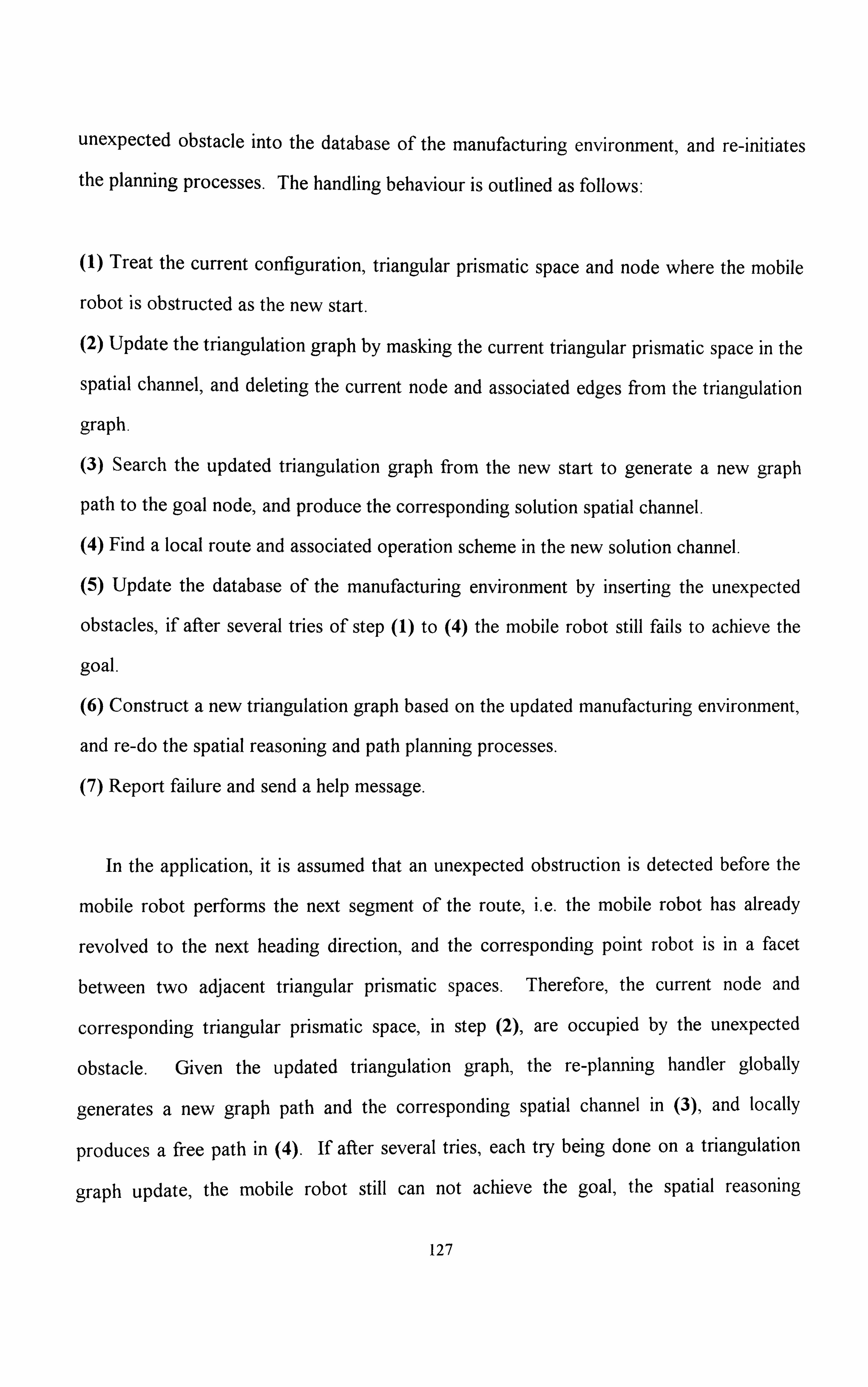
unexpected obstacle into the database of the manufacturing environment, and re-Initiates the planning processes. The handling behaviour is outlined as follows.
(1) Treat the current configuration, triangular prismatic space and node where the mobile
robot is obstructed as the new start.
(2) Update the triangulation graph by masking the current triangular prismatic space in the
spatial channel, and deleting the current node and associated edges from the triangulation
graph.
Search the updated triangulation graph from the new start to generate a new graph
path to the goal node, and produce the corresponding solution spatial channel.
(4) Find a local route and associated operation scheme in the new solution channel.
(5) Update the database of the manufacturing environment by inserting the unexpected
obstacles, if after several tries of step (1) to (4) the mobile robot still fails to achieve the
goal.
(6) Construct a new triangulation graph based on the updated manufacturing environment,
and re-do the spatial reasoning and path planning processes.
(7) Report failure and send a help message.
In the application, it is assumed that an unexpected obstruction is detected before the
mobile robot performs the next segment of the route, i. e. the mobile robot has already
revolved to the next heading direction, and the corresponding point robot is in a facet
between two adjacent triangular prismatic spaces. Therefore, the current node and
corresponding triangular prismatic space, in step (2), are occupied by the unexpected
obstacle. Given the updated triangulation graph, the re-planning handler globally
generates a new graph path and the corresponding spatial channel in (3), and locally
produces a free path in (4). If after several tries, each try being done on a triangulation
graph update, the mobile robot still can not achieve the goal, the spatial reasoning
127

processes will be carried out again in (5). A new triangulation graph is constructed, and the planning is performed again in (6). Similarly, if after several tries, each try being done
on an environmental datebase update, the mobile robot fails to achieve the goal, the program terminates with an appropriate message in (7).
4.6. SUMMARY
In this chapter, a new approach for planning collision-free navigation for mobile robots
in a manufacturing environment has been presented. This planning approach is based on triangulation from computational geometry. Since triangles are easy to handle, an
approach of this nature simplifies the task of planning coll'sion-free navigation.
A navigation planning task is divided for mobile robots into four sub-tasks- (1) modelling the manufacturing environment as a group of numerical data in a suitable
mathematical construction accessible to the computing system of the mobile robot;
(2) transforming the mathematical model to a graph;
(3) applying a graph searching algorithm to the graph to produce a solution graph path,
(4) interpreting the solution graph path as a navigation proposal for the mobile robot.
Given a mobile robot and manufacturing environment, the configuration free space of
the mobile robot is constructed. The planning approach then models the configuration
free space of the mobile robot as a connected set of triangular related cells, and builds a
triangulation graph accordingly. This triangulation graph implicitly represents the
topological connectivity of the configuration free space. If the start and goal
configurations, denoted by S and G, are given in a connected sub-set of the configuration
free space, a corresponding graph path can be produced on the triangulation graph, using
an optimal graph searching algorithm. This solution graph path is a journey indicating a
globally preferable movement trend of the mobile robot. Since the journey physically
represents a spatial channel in the configuration free space, which contains S and G, there
128

are many free paths from S to G, available in the journey. A solution path connecting S
and G with maximum clearance is locally planned in the journey channel, using the discrete
navigation mode. The route and associated operation scheme for the mobile robot to
navigate are finally derived from the path.
Due to the clearance advantage of the journey, the solution path is also adjustable to
avoid unexpected obstacles. Handling behaviours capable of proposing alternative paths
to avoid unexpected obstacles are developed, and organised in a hierarchical structure. When an unexpected obstacle has been encountered, the mobile robot waits for a moment in case the obstruction will be cleared automatically. Otherwise, the obstruction is
propagated to a higher level of handler, which plans a tangent or triangulation detouring
path in the journey, through the clearance space, to locally avoid the obstruction. At the
highest level of the handlers, the triangulation graph and database for the manufacturing
environment are updated, and a global re-planning process, including spatial reasoning and
path searching, is carried out.
At the executing stage of the navigation strategy, the mobile robot will follow the
planned route and operation scheme, as required by the motion and sensing commands, to
perform the navigation in the manufacturing environment.
129
CHAPTER FIVE EXECUTING: MOTION CO- ORDINATING AND SENSING
This chapter deals with the executing aspect of the navigation strategy. The proposals
produced at the planning stage are to be implemented in practical scenes. The
implementation is carried out in three steps:
(1) Computer. A graphical user interface tool is developed for the host personal
computer to interactive y communicate with the user through its visual di 'splay unit, by
graphically demonstrating the planning procedure and results.
(2) Manipulative robot and camera. The planned navigation is simulated, using the
MOVEMASTER-EX manipulative robot. The camera system (Data Translation Inc. and
Prostab International Limited) is used to attain the initial environmental information.
(3) Mobile robot and ultrasonic sensors. The navigation planning approach is
implemented in the B 12 mobile robot, using six ultrasonic sensors for external sensing.
Whatever system is used for the implementation, motion co-ordinating and sensing
mechanisms are two major subjects to be considered at the executing stage. Given a
planned route and associated operation scheme, the motion co-ordinating mechanism is to
compose and initiate appropriate motion instructions at appropriate moments, which can
direct system behaviours to as accurately as possible perform the route and operation
scheme. The sensing mechanism is to provide on-line navigation-related information for
130

the system to make decisions, performance corrections and further plans. However, the aim of the implementation is to prove the feasibility of the triangulation based navigation planning approach in manufacturing environments. Only minimum basic equipment is used for external sensing, so that the advantages of the planning approach can be verified.
Different systems use different types of mechanisms for motion co-ordinating and
sensing. Therefore, the implementation techniques in the three steps are system specific, and are described individually.
5.1. GRAPHICAL USER INTERFACE The flexible material transport system itself is not likely to understand a user-requested
task. Therefore, a tool for graphical user interface is developed, which converts
the user's input to the system's knowledge, and the system's responses to graphical
displays for the user's convenience. The flexible material transport system, that waits for
the user is thus a collection of machinery (hardware) and programs (software) to be
instructed or initiated. 'functions of the graphical user interface tool may be partially The
achieved by using a commercial CAD/CAM package. A major task is to
transform/transfer the database foring, used in the CAD/CAM package, to a compatible
set of the flexible material transport system [ 12]. However, the graphical user interface
tool is developed in order to understand the internal communications mechanism among
the component systems of the flexible material transport system.
The development of the graphical user interface tool is to put the user into direct and
interactive communication with the flexible material transport system, through the visual
display unit (screen) of the host personal computer. Using the tool, the user can interface
with the flexible material transport system, operate every component system individually,
and compose control programs off-line for automatic operations. The turnaround time
131

and costs for designing and re-designing layouts of a manufacturing environment, and finding and adjusting the system performance, can be reduced.
5.1.1. Software Structure
The graphical user interface tool supports two modes of interaction to operate the
flexible material transport system, which are the direct and indirect modes. They are distinguished by whether the user or the navigation planner (planning approach) is in
control of the system's behaviours.
(a) Direct interaction mode. In this mode, the tool has two functions-
(a. 1) The user can create and edit an environmental layout. Geometrical features and
spatial arrangement of the contained objects, which are to be avoided by the mobile robot,
can be illustrated on-line on the computer screen.
(a. 2) The flexible material transport system is to work under direct supervision of the user.
No intelligent or decision making task is done by the system itself All component systems
of the flexible material transport system are at their standby states, waiting for instructions
from the user. Only one instruction can be executed at a time since the host computer is a
serial machine. All entered instructions are carried out sequentially, and each is responded
immediately. Any response produced by the flexible material transport system is a result
of the user's activities.
(b) Indirect interaction mode. On the other hand, the flexible material transport system
is controlled by the navigation planner, based on the developed triangulation planning
approach. In the indirect mode, there are also two functions:
(b. 1) A function for computational graphical simulation is developed, in order to preview
the planned navigation for the mobile robot in a given environmental layout. The
computer is graphically simulating the navigation performance of the mobile robot on the
132

screen. This function enables the user to enter variable information, and to preview possible navigation results correspondingly. The user can also monitor the steps of the
navigation planning approach as it progresses. As a result, much unnecessary trial-and-
error implementation in practical scenes can be saved. Due to the rapid response of the
computational graphical simulation function, an environmental layout can be designed,
tested, and edited rapidly on the host computer through this function.
(b. 2) The mobile robot can navigate to the goal posture itself without direct human
interference, until any occurrence of non-recoverable errors. The navigation result,
consisting of a sequence of "current" postures of the mobile robot, is on-line graphically
displayed on the computer screen for the user's reference.
5.1.2. Technigues and Results
As described in chapter two, the hardware set-up of the flexible material transport
system has been completed. The manipulative robot, camera vision system, and mobile
robot with six ultrasonic sensors are connected to the host personal computer through the
parallel cable, internal bus board, and serial cable respectively. The flexible material
transport system is ready to operate without further hardware modification. To develop
the graphical user interface tool, a major task required is to produce software for
communications and control) which can drive each of the component systems and
mechanisms from the host computer.
The software is produced using the Visual BASIC programming language. A 640 by
480 resolution is defined to the computer's visual display unit to construct the graphical
environment for computational simulation. To prevent any disaster happening, the
emergency buttons, provided by manufacturers of the component systems, are treated as
the first priority interruption for all processing. When any emergency button of the
component systems is pressed , the flexible material transport system is immediately
133

brought to a stop. A reset procedure is necessary to activate the flexible material transport system again.
5.1.2.1. Direct Interaction Mode
The direct interaction mode is developed for designing layouts of a manufacturing
environment, testing system commands and reactions', and previewing operational
procedures.
(a) To achieve the (a. 1) function of section 5.1.1, a drawing program is produced, using
the versatile graphic commands provided by the progranuning language. The drawing
program can graphically display an environmental layout on the computer screen, by
combining geometrical shapes, such as points, lines, rectangles, circles, arcs, and wedges,
to form a variety of screen images. Since an environmental layout is designed by the user v
as a set of numerical data, the drawing program manipulates the data to produce a 0A-k; 'Az
clear and simple picture. The picture illustrates the set of numerical data, and thus the
environmental layout. This function can communicate facts and ideas that would be
abstractly difficult for the user to grasp from the equivalent set of numerical data.
(b) As to the (a. 2) function of section 5.1.1, a specific communications program is
produced, enabling the user to interactively instruct the flexible material transport system.
The communications program is completed by knowing the format and protocol for data
transmission among the component systems. Apart from the serial commumcatIons cable
produced to connect the host computer and the mobile robot with six ultrasonic sensors, a
communications setting of 9600 Baud Rate, 8 Data Bits, I Stop Bits, None Parity Check
and Xon/Xoff Flow Control is required to transmit signals mutually. In addition, since a
parallel communications cable has been produced to connect the manipulative robot with
the host computer, no such serial communications setting is required. However, if serial
134

communications is used between the manipulative robot and host computer instead of
parallel communications, 9600 Baud Rate,, 7 Data Bits, 2 Stop Bits, Even Parity,
Xon/Xoff Flow Control, and Enable Parity Check are assigned to meet the default
configurations of the manipulative robot for serial communications.
Technically, every communications port of the host computer is managed as a random
access file [67][69] in the communications program. In addition to the hardware cable
configurations and the communications settings, interpretation sub-programs are also
produced to convert the transmitted digital signals, complying with the ASCII code, and
associated data protocols to languages or symbols understandable to the user. The
communications program is invoked to function as a terminal emulation tool, which makes
the host computer act as a full duplex operational terminal for the flexible material
transport system, echoing all user entered instructions.
5.1.2.2. Indirect Interaction Mode
The indirect mode of interaction is based on the programs produced for the direct
mode, and on the previously developed triangulation based navigation planning approach.
The software begins by manipulating the input information about the environmental
layout, in order to identify the free work space where the mobile robot can move freely.
The free work space is then given to the planning approach, as a polygonal region with
polygonal holes, to be processed.
(a) There are many situations in which understandiný erformance of a dynan-fic system, ,L
without practically running the system in the real world , is required. For example, the real
world version might perform too slowlyl or yield potentially devastating consequences. In
these situations, it is better to reason how the system would behave, than to observe its
behaviours. The computational graphical simulation function, described in (b. 1) of section
5.1.1, is for this purpose. This function is achieved by using a circular image, moving on
135

the visual display unit of the host computer, to perform the behaviours of the mobile
robot. This circular image is controlled by an executing approach, simulating the
executing mechanism of the mobile robot. By intely-ating the executing approach with
the triangulation planning approach, the circular image can perform the planned route and
associated operation scheme. zr, -&441ýlon, all intermediate processes, including layout
defining, free space constructing, bridge building, triangulating, triangulation graph
searching, global journey generating, and local route and associated operation scheme
producing, are displayed on the screen sequentially. Although the graphical simulation
function is not able to replace the real implementation in the mobile robot, the function
provides a useful tool for reasoning about possible consequences due to an input
environmental layout. This function is an important design aid. Figure 5.1 illustrates a
simulation example.
obstacle
G obstacle
mobile robot Eobstacle
obstacle S
-------------------- obstacle
1. layout designing
2. free space constructing
3. bridge building
4. triangulating
S. triangulation graph searching
6. journey generating
7. route and operation scheme producing
Figure 5.1. Graphical user interface
(b) The (b. 2) function of section 5.1.1 is only invoked when the mobile robot itself is
executing the navigation. Given a layout of a manufacturing environment, the mobile
robot navigates along the planned route and associated operation scheme. Due to
136

uncertainties, the practical performance of the mobile robot is not likely to be identical to
the theoretically planned navigation. By manipulating the information produced by on- board sensors, the "actual" postures of the mobile robot with respect to the defined world
co-ordinate frame, at instants of sensor-triggering (sampling time), are calculated. These
postures are graphically displayed on the screen. Since the sampling time is discrete,
postures between two instants of sensor-triggering are linearly interpreted. As a result,
the actual navigation performance of the mobile robot, in the given manufacturing
environment, is illustrated. Although the displayed actual navigation result may not
precisely describe the real performance of the mobile robot, due to uncertainties, sensor
insufficiency and linear interpretation, the displayed result can still be a useful reference.
5.2. SIMULATION USING MANIPULATIVE ROBOT AND
CAMERA
In addition to the computational graphical simulation function developed for the
graphical user interface tool, another simulation environment is constructed. The purpose
of the construction is to set up a quick-responding and small-scaled simulation system,
which can be used to practically test the triangulation planning approach. It is also to
identify possible factors, which could affect the mobile robot implementation. This
construction is a correlated project with a fellow research student, Mr. Y. Zhu, who is
investigating image processing issues [137], both theoretically and experimentally.
5.2.1. System Construction
The simulation system is constructed, using the manipulative robot and vision camera
of the flexible material transport system. The working domain of the simulated
manufacturing environment is defined by a camera stand. The base board of the camera
stand represents the "floor" of a manufacturing environment. Several pieces of plastic
137

plate are placed on the base board to represent possible obstacles in a real manufacturing
environment. The plastic plates have polygonal shapes and 2mm thickness, and are
allocated according to a designed environmental layout.
The vision camera is fixed overhead, 70cm above and with its optical axis
perpendicular to the base board, to cover the working domain. Images grabbed by the
vision camera are processed to produce useful information about the environmental layout. This information is used as the input to the developed navigation planning
approach. Output of the navigation planning approach is used to drive the manipulative
robot. The manipulative robot is located along side the base board. A pencil is held by
the gripper of the manipulative robot to draw the planned navigation trajectory on the base
board. Figure 5.2 illustrates the constructed simulation environment.
base board
Figure 5.2. Simulation environment
5.2.2. Technigues and Results
Having constructed the simulation system,, the triangulation based navigation planning
approach is implemented. First, an image of the environmental layout is grabbed and
processed by the vision camera to abstract useful information. Once the start and goal
points have been assigned, the triangulation planmng approach can produce a route and
138
tasks planning approaches
associated operational scheme in the environmental layout. The route and associated
operational scheme is finally performed by the MOVEMASTER-EX manipulative robot. When using the simulation system to execute the planned result, three co-ordinate
systems are involved-
(1) the co-ordinate system for planning navigation,
(2) the co-ordinate system for co-ordinating motion,
(3) the co-ordinate system for sensing.
The three co-ordinate systems are illustrated in Fig. 5.2. Since the simulation system has
to work harmonically, data signals are transferred from the camera vision system to the
navigation planner, and from the navigation planner to the manipulative robot. Data with
respect to one co-ordinate frame have to be transformed to their equivalent values with
respect to the other co-ordinate frame, before they are processed by the corresponding
system. Transformation among the co-ordinate systems is required.
The co-ordinate system for planning navigation is defined by superimposing a Cartesian
co-ordinate system on the working domain, or the base board of the camera stand. This
co-ordinate frame is intuitively settled, complying with the right-hand rule and I-I scale
rate, and has its origin at a corner of the base board. Data produced by the camera vision
system have to be transformed into this co-ordinate system, in order to be exported to the
navigation planning approach.
5.2.2.1. Motion Co-ordinating
The motion co-ordinating mechanism of the simulation system controls the
manipulative robot to draw, using a pencil, in the simulated manufacturing environment,
or on the base board. In other words, it is to find the necessary torque to actuate the joint
motors at every instant of sampling time. Three levels of controllers [401 are included in
the motion co-ordinating mechanism of the manipulative robot-.
139

(1) Supervisor level controller. A supervisor is either a human user or the planning
approach. The supervisor level controller provides instructions for the manipulative robot to perform the desired behaviours.
(2) Command level controller. The command level controller converts the instructions,
from the supervisor level controller, to voltage values, which are used by the Joint level
controller.
(3) Joint level controller. The joint level controller manages angular movements of the
robot joints, by using position servos for the joint motors.
The manipulative robot is a commercially off-the-shelf and ready-to-use industrial
system. It has a control unit supporting the command level and joint level controllers for
reliable performance. Therefore, the supervisor level controller is produced to complete
the motion co-ordinating mechanism. The supervisor level controller is used mainly to
convert the output from the triangulation based navigation planner to a combination of
available robot motions. To draw on the base board smoothly, the gripper of the
manipulative robot, which holds a pencil, is always kept perpendicular to the base board.
However, some working space of the simulated manufacturing environment is sacrificed
due to this restriction.
The manipulative robot has a manufacturer defined Cartesian co-ordinate system.
Comparing it with the Cartesian co-ordinate system for planning navigation, the co-
ordinate system for motion co-ordinating has the same unit scale. Since the manipulative
robot is fixed along side the simulated manufacturing environment, making the two
Cartesian co-ordinate systems parallel, the transformation between the two co-ordinate
systems is constant.
To deal with the position repeatability and line-following difficulty, a number of
intermediate points are introduced to all straight-line routes, in order to perform the
planned discrete navigation. The more number of intermediate points, the smoother and
closer the performance is to the planned discrete navigation. However, more executing
140

time is also required. In addition, a tolerance width, which is about 3mm and experimentally produced, is defined to the navigation route. Any gap, between obstacles in the simulated manufacturing environment, narrower than the tolerance width is assumed obstructed. Gaps are determined by the heights of the triangular regions, produced by the triangulation planning approach. Figure 5.3 illustrates the implementation techniques.
tolerance width
planned route actual route
3mm (not to scale)
(a)
obstacle obstacle
; route gap
!
obstacle (b)
Figure 5.3. Intermediate points and tolerance width
5.2.2.2. Sensing
The vision system comprises a camera, processing boards, a monitor, and lighting
equipment. The camera is placed above the simulated manufacturing environment. After
taking an image of the environment, the camera returns a matrix of pixels. Each pixel
represents a voltage proportional to the light level of its corresponding part in the image.
Since the vision system is monochrome, the pixels are quantified by 8 bits of discrete grey
levels, black through to white. Information about the environment is inferred by
processing the pixel data. Understanding an image usually requires a sequence of complex
processing and a large amount of computations. In addition, the processing must raise the
quality of the raw data to the standard required by the navigation planner.
A grey-level representation of the matrix of pixels may not truly stand for the
corresponding environmental image. This may be due to factors such as reflectance
function, illumination, shadowing, electrical noise, visual noise, distortion, orientation of
obstacles, etc. Since the simulation system is mainly to test the feasibility of the navigation
141

planning approach in practical scenes, attempts are made to technically eliminate problems
caused by these factors.
Four lamps of the lighting equipment are positioned around the base board to provide
sufficient light sources. Therefore, the simulation system has illumination bright enough to deal with the suffering from varying light condition and noise. The distortion effect is
minimised, by excluding the boundary area of an image from processing, and setting the
overhead camera to point perpendicularly downward to the base board.
The camera is fixed 70cm high above the working domain. Since the camera is fixed,
the co-ordinate system for sensing can be calibrated to refer the co-ordinate system of the
navigation planner. The two co-ordinate systems are parallel, and have the same
directions but different unit scales. At 70cm height, the camera produces a 40cm by 40cm
square of coverage on the base board. Since the co-ordinate system of the camera, or the
resolution for processing an image, is a square of 512 pixel by 512 pixel, the
transformation rate between the co-ordinate systems for sensing and navigation planning
can be produced; I cm= I 2.8pixels.
In addition, all obstacles in an environmental image are assumed to have zero heights,
when the edge-detection processing is performed to identify obstacle boundaries. That is,
Thi it is assumed that environmental images are taken from an infinitely far di is
orthographic projection assumption avoids the complexity of distinguishing three
dimensional obstacles from a two dimensional image. However, information about an
obstacle thus produced is slightly larger than the real one. The thin thickness of the plastic
plates is to submerge the shadowing noise.
As to the effect of obstacle orientation, different positions and orientations of an
obstacle on the base board may result in irregularity of obstacle edges in the corresponding
pixel representations. This problem is handled by assuming that all obstacles in the
working domain are polygons. When processing an environmental image, boundaries of
obstacles are produced, by first identifying pixels with discontinuity in grey levels. Each
142

obstacle boundary consists of a connected set of pixels. By setting a width threshold,
consecutive pixels within the width threshold are represented by a straight-line segment, which is tangent to these pixels. Boundary information about the 'polygonal' obstacles is finally produced. After processing, an obstacle may present a 6-gone at a position and orientation, but an 8-gone at another. Figure 5.4 illustrates an example. The information
produced is the input to the navigation planner, if the camera image system provides the
only environmental information.
actual boundary
I
Figure 5.4. Pixel boundary
5.2.2.3. Results
A simulation system is accomplished, using the manipulative robot and the vision
camera of the flexible material transport system. The camera scans the simulated
manufacturing environment, and passes the produced obstacle information to the
triangulation based navigation planner. A navigation is then planned for the manipulative
robot to execute. The camera and manipulative robot being fixed, with respect to the
camera stand, enables calibration of the three co-ordinate systems to be made. The zero-
height obstacle model introduces a gross navigation effect, which slightly enlarges
obstacles, and enhances clearance for the planned navigation.
The feasibility of the triangulation based planning approach, in a small-scaled simulated
manufacturing environment, is verified. The simulation system also helps identifying
possible factors, which could affect the mobile robot implementation In addition,
143
produced boundary
hardware of the simulation system can be used to test other navigation planning approaches. However, expensive computational costs for processing vision images (approximately 1.5 minutes) are the main disadvantage of the simulation system. A real- time performance may be achieved by improving approaches, techniques, and hardware for processing vision images, which reduces the time required to update the input to the
navigation planner.
5.2-3. Desijzn and Simulation
The graphical user interface tool, running on the host personal computer, and the
simulation system,, using the manipulative robot and the vision camera, are both developed
to model the navigation performance of the mobile robot in a manufacturing environment.
Simulation represents a particularly useful function for reasoning about a possible spatial
arrangement of obstacles, and the corresponding navigation results, that avoids the
imprecision of intuition or prediction. Also, it provides a more practical formulation than
mathematics for modelling the navigation planning approach.
In the development of the flexible material transport system, the two simulation
functions are both regarded as important aid tools in designing layouts of a manufacturing
environment. If simulation runs can conveniently test, or verify, the navigation processes
of the mobile robot in a simulated environmental layout, then, in situations where the
structural characteristics of the corresponding real manufacturing environment are user
controlled, the simulation information can be used as a basis for judging and modifying the
layout structure of the real manufacturing environment.
The design of a physical system is often accomplished by a cycle of activities [138],
including phases that construct models, test behavioural consequences of the models by
simulation, diagnose the causes fQrpoor behaviour in terms of design weakness, and
propose model changes. Ideally, a cycle of such activities should produce a system with
the desired behavioural properties.
144

Similarly, designing structural layouts of a manufacturing environment is also an iterative procedure. Candidate layout designs are proposed first, according to the
manufacturing target. Their Implications for the mobile robot navigation are followed by
simulation. Selection or modification on these candidates is then madel based on the
simulation results. The design cycle is repeated until a layout design is decided, which has
satisfactory simulation results of the mobile robot navigation. The designed environmental layout is finally employed to construct or re-locate the physical objects in the
manufacturing environment. The design cycle is illustrated in Fig. 5.5. Using the two
simulation tools to design a layout of a manufacturing environment, implementation costs
and damages due to trial-and-error practices by navigating the mobile robot can be
reduced.
graphical user interface tool
simulation system
I
mobile robot implementation
(b)
Figure 5.5. Design cycle
The final step is to implement the triangulation based navigation planning approach to
the mobile robot. The manufacturing environment is constructed according to the
designed layout and simulation results. In the implementation, the motion co-ordinating,
sensing, and managing mechanisms are required to execute the planned navigation.
145
exit

5.3. MOTION CO-ORDINATING FOR MOBILE ROBOT To perform the planned navigation, the mobile robot must move itself from the start
posture to the goal posture in a co-ordinated fashion,, and along the prescribed route and
associated operation scheme. Therefore, an important concern at the executing stage is to develop a motion co-ordinating mechanism, which can automatically compose a sequence
of motions of the mobile robot. This sequence of motions is then converted to proper
motor control profiles, used to drive the translation (wheeling) and rotation (steering)
motors. In other words, the motion co-ordinating mechanism is to derive systematic
motor control profiles for the mobile robot to execute the planned route and associated
operation scheme.
5.3.1. Structure and Techniques
As described in chapter two, the mobile robot has a translation and a rotation servo
loop. Each servo loop consists of a motor and an encoder, and can be independently
operated in velocity, position, power, and limp modes, within a range of velocities and
accelerations. As a result, the three wheel driving and three wheel steering mechanism
gives the mobile robot an om-ni-directional travelling capability. Also, this synchronous
mobile mechanism provides the robot system with two modes of navigation; discrete and
continuous.
5.3.1.1. Structure
Whatever navigation mode is performed by the mobile robot, three levels of
hierarchically organised controllers are used to construct the motion co-ordinating
mechanism, as those of the simulation system in section 5.2.2.1.
(a) Motor level controller [431. Two motor level controllers are at the lowest level of
the motion co-ordinating mechanism; one for translation and the other for rotation. Each
146

consists of control circuits for managing a motor and an optical encoder, and forms a
servo loop. The motor level controllers work by controlling state vectors of angular
position and angular velocity for the motors, and integrating signals from the optical
encoders.
(b) Command level controller. The command level controller converts the motion
instructions, from the supervisor level controller, to voltage values. The voltage values
are used by the motor level controllers to drive the two servo loops. The command level
controller also produces an encoder count for each of the servo loops through
accumulating encoder signals, captured by the corresponding motor level controller.
(c) Supervisor level controller. The supervisor level controller describes the route and
associated operation scheme, produced by the navigation planning approach, as a set of
motion instructions of the mobile robot. It also informs the navigation planning approach
the current posture and failure performance of the mobile robot. Using the produced
motion instructions, the mobile robot can perform the planned navigation.
desired navigation ý Tposture estimate & failure
Fsupervisor level controller motion instructions jf
encoder readings
command level con! oller driving signals eý 5 driving signals encoder sipals
----------------------------------- ---------- ------------------------------------- ....... m to level controller motor level controller
encoder
----------------- ------------------- ---------------------------------------- ---------------------- -------------------- translation rotation
Figure 5.6 Motion co-ordinating mechanism
147

Figure 5.6 illustrates the hierarchical structure of the motion co-ordinating mechanism. The control unit of the B 12 mobile robot has the functions of the motor level controllers. Also, a manufacturer-defined operation system is pre-loaded in the mobile robot. This
operation system consists of a set of control commands for the two servo loops, and can be used to function as the command level controller of the mobile robot. Therefore, the supervisor level controller is produced to complete the motion co-ordinating mechanism.
5.3.1.2. Techniques
A major concern for the development of the supervisor level controller is to achieve a
prescribed navigation, which is expressed in the co-ordinate system of the navigation
planning approach, or of the manufacturing environment. Two principal functions are included in the supervisor lever controller; to perform the prescribed navigation and to
make posture estimates with respect to the manufacturing environment while navigating.
(a)Performing prescribed navigation. Methods enabling the mobile robot to perform
the two modes of navigation are developed. Technically, discrete and continuous
navigation can be accomplished by the following control methods:
(a. 1) The discrete navigation mode is achieved, if the translation and rotation servo loops
are sequentially controlled in a scheduled order. The overall navigation is divided into a
sequence of performance intervals. Each performance interval is formulated by executing
velocity, acceleration, displacement, and time of either the translation or rotation servo
loops. One motor is only initiated, when the other stops. Therefore, the mobile robot can
move forward and backward, or revolve on its central axis, but not together in the same
performance interval. In this mode, a navigation trajectory of the mobile robot is
presented as a sequence of move- stop-revolve movements. Given the geometrical
parameters of a prescribed discrete navigation, time parameters are used by the supervisor
level controller to compose the velocity and acceleration functions for the performance
148
intervals, and to co-ordinate the translation and rotation motors. A desired discrete
navigation can always be described as a sequence of motion instructions of the mobile
robot.
(a. 2) The continuous navigation mode is achieved by simultaneously controlling the two
servo loops of the mobile robot. A curve navigation trajectory is presented by the mobile
robot in the continuous navigation mode. To perform a prescribed continuous navigation,
a set of translation and rotation motions of the mobile robot are carefully combined, in
order to match the performed trajectory with mathematical features of the prescribed
curve route. The combination is a result of complicated and precise computations. Time-
based parameters are used to control the translation and rotation motors. However,
translation- displacement based parameters are considered for controlling the rotation
motor, if the given curve route is characterised by a curvature function. That is, the
rotation motor is controlled by the travelling distance of the mobile robot. The general
expression for curvature of a curve route is K=dE)IdS, where S is the route-length
(travelling distance) variable, and 0 is the angle of the tangent to the route (the heading
direction of the mobile robot since its centre of rotation is following the route). An
arbitrarily prescribed curve route may not be feasible due to kinematics constraints of the
mobile robot.
(b) Making posture estimate. To perform a prescribed navigation, expressed in the co-
ordinate system of the planning approach, the supervisor level controller has to make
posture estimates of the mobile robot, with respect to the manufacturing environment.
The posture-estimation is done by a dead reckoning method, mainly using readings from
the two optical encoders. Assuming that at time to, the mobile robot is at an initial posture
(Xo, Yo, Oo), with respect to the manufacturing environment. In the triple, (Xo, Yo) is the
position of the revolving axis (centre of rotation), and Oo the heading direction, of the
149

mobile robot. This dead reckoning method makes posture estimates for the two
navigation modes by the following approaches-
(b. 1) In the discrete navigation mode, the translation and rotation servo loops are
sequentially controlled in a scheduled order. One motor is only initiated when the other
motor stops. When the mobile robot is performing a discrete navigation, the overall
performing time is divided into n time intervals (tO, tl, t2,..., tn), and each time interval
equivalently represents a performance interval as illustrated in Fig. 5.7. During a time
interval Ati, Ati=ti-ti-j and ha! ýn, either the translation or the rotation servo loop is
working. Since a time instant tj (O: q':! ýn), dividing the performing time, is also a sensor
sampling time, encoder readings of the translation and rotation servo loops at tj are
fetched. Therefore, Si and 0j, respectively representing the translation and rotation
positions at tj, can be produced from the encoder readings.
t
mobile robot tI A si+ C. C. W. + Aý j
i+I ýO As =0
. W. - discrete navigation X 6=0
manufacturing environment
Figure 5.7. Time interval and discrete navigation
Let (So, Si, S2,..., Sn) and be the position ntervals for translation and
rotation respectively, corresponding to (to, b, t2, ---,
tn), ý0:: -E)O- Furthermore, let (X, Yi, Oi)
be the posture estimate of the mobile robot with respect to the manufacturing
environment, at a sampling time ti, tie Ito, tI, t2,..., tn). (Xi, Yi, E)i) can be produced by the
following equations:
E)i=E)o+ 1. =,
Aok=oo+ I Aok=oi lk lk=l
150

Xi=Xo+lk=l (ASk XCOSE)k-])= XO+ lk=l k -1 (ASk XCOS(00+1, =,
Aoi))
I. Yi=Yo+lk=l (ASkxsinE)k-, )= I. Yo+lk=, k-I (ASkxsin(E)o+l,
=, Aoi))
where Aýk4k-ýk-j and ASk=Sk-Sk-j.
Similarly, at an arbitrary time instance ti, ti-i<t1<ti and tiGtti, t2, ...
tn), the posture
estimate (Xl, Yi, 01) is-
Or--Oi-i+Aoi--ol
Xi--X-j+ASlxCOSE)i-i
Yi--Yi-j+ASixsinOi-,
where *--ý1+-i and AS1--Si-Si-i respectively represent the displacements of rotation and
translation from ti-j to ti.
(b. 2) The continuous navigation mode is to simultaneously control the two servo loops of
the mobile robot. It is also formulated from the velocity, acceleration, displacement and
time inputs to the translation and rotation servo loops. Let Vi, o)j, ýi and Si respectively
represent the instantaneous translation velocity, rotation velocity, heading direction and
travelling distance of the mobile robot at time ti. Let (X-, Y,, Oi) be the posture estimate of
the mobile robot with respect to the manufacturing environment at ti. (Xi, Yi, Oi) can be
theoretically calculated by the following equations- ný "040
ný Oi=E)o+Aý-E) codt--ýi or to
Oi=Oo+ si Kds and Si= ti vdt f sso soyto
where K is a curvature function. The variations of X and Y at the neighbourhood of time
t are AX, and AY, respectively
AX=ViCOSOiAt
Ayi=visinE)iAt
151

Therefore, the X and Y positions of the mobile robot with respect to the manufacturing environment at time ti are:
Xi=X ti VCOSOdt olto
Yi=Y ti vsinOdt olto
The dead reckoning method uses encoder readings to make posture estimates of the
mobile robot. Practically, fetching and processing encoder readings takes time, and the
time intervals between sampling instants have to be considered. In other words, when the
mobile robot is performing a continuous navigation, an interpretation model of the curve
route, between two sampling instants, has to be used instead of the theoretical model. As
a result, the following equations are proposed to make practical posture estimates in a
continuous navigation: la VW4
X=X-j+ASiCOS((ýi+ýi-i)/2)
Yi=Yi-i+ASiSin((ýi+ýi-, )/2)
if ti and ti-i are the current and previous sampling instants, and AS, =S, -S, -j- Obviously, the
proposed equations use a heuristic model for the continuous navigation mode, and the
mobile robot can only make approximate posture estimates. However, this interpretation
model provides a practical means for localising the mobile robot in continuous navigation.
Figure 5.8 illustrates an example of continuous navigation.
AS it
`00ý I, manufacturing environment
x
Figure 5.8. Continuous navigation
152

The dead reckoning method, using readings from the optical encoders, is very economical to implement. However, making posture estimates by this method is recognised to be prone to modelling errors, and noises from encoder quantization and floor roughness. The mobile robot requires other methods to make posture estimates, as a supplement to the dead reckoning method, at least on an occasional basis.
5.3.2. Physical Features
In order to develop the motion co-ordinating mechanism, physical features of the
control unit of the mobile robot (the command and motor level controllers of the motion
co-ordinating mechanism) have to be realised.
There are incremental optical encoders mounted on both the translation and rotation
motors, providing dead reckoning and feedback control for the mobile robot. Each optical
encoder provides 500 counts per motor revolution. Since the control unit zeros the
encoder counters at every system reset, angular positions of the motors can be measured
cumulatively from the reset moment. By using constant time intervals, and consistently
checking the variations of angular position and angular velocity over the time intervals, the
control unit can maintain the motors at the desired angular velocity and angular
acceleration respectively.
The motion commands and parameters, provided by the manufacturer, are motor based
and in hexadecimal notation. Therefore, they have to be converted into the notation which
is recognisable to the supervisor level controller.
5.3.2.1. Translation
To transmit work from the translation motor to the wheels, three gear sets are available
to drive the mobile robot; 71: I for light loads and high speed, II-I for medium loads and 3
medium speed, and 14.1 for heavy loads and slow speed The gear sets serve for work
153

transmission as well as speed reduction. Each ratio is a speed reduction rate, representing
the number of revolutioncof the translation motor per wheel revolution.
Given a gear set, the travelling distance of the mobile robot, D, can be calculated by
the following equations:
D=2 x7r xRxRev. w=2 x 7c xRx (Rev. m--: --Rate)=2 x 7c xRx (Count-5 00--Rate)
where R, Rev. w, Rev. m, Rate, Count and 500 respectively represent the wheel radius
(4.15cm), number of revolution of the wheels, number of revolution of the translation
motor, reduction rate, counts of the translation optical encoder, and encoder counts per
motor revolution. For example, the three reduction rates, 14: 11 11 A and 71-1, enable the 3
mobile robot to travel 1000cm by 268267,210302 and 139882 counts (decimal) of the
translation optical encoder. In addition, an encoder count in decimal notation has to be
converted to a corresponding value in hexadecimal notation, before it is used to command
the mobile robot. Table 5.1 is a conversion table for translation distance versus encoder
count. At present, the 11: 1 gear set is used, enabling the mobile robot to travel
approXimately 26cm for every II motor revolutions.
r gear set
14: 1 14: 1 11: 1 11: 1 1 1 7 1 7 :1
count 3 3 distance (dec. ) (hex. ) (dec. ) (hex. ) (dec. ) (hex. ) lCm 268 10C 210 D2 140 8C
10CM 2683 A7B 2103 837 1399 577
100CM 26827 68CB 21030 5226 13988 36A4
1000CM 268267 417EB 210302 3357E 139882 2226A
Table 5.1. Distance travelled versus encoder count
5.3.2.2. Rotation
As to the transmission system employed by the rotation motor, a 236.4-1 reduction
ratio is provided. Every 236.4 revolutions of the rotation motor the mobile robot revolves
360 degrees about its central axis. Therefore, there are
154

236.4x5OO=l 18200 encoder counts (decimal)
for every 360 degrees of change of the heading direction. In other words, there are
118200-360=3281 encoder counts (decimal) 3
per degree of change of the heading direction.
Similarly, an encoder count in decimal notation has to be converted to a corresponding
value in hexadecimal notation, before it is used to instruct the mobile robot. Table 5.2 is a conversion table for rotation displacement versus encoder count.
degree dec. hex degree dec. hex. degree dec. hex. 10 3283 CD3 130 42683 A6BB 250 82083 140A3 20 6567 19A7 140 45967 B38F 260 85367 14D77 30 9850 267A 150 49250 C062 270 88650 15A4A 40 13133 334D 160 52533 CD35 280 91933 1671D 50 16417 4021 170 55817 DA09 290 95217 173F 1 60 19700 4CF4 180 59100 E6DC 300 98500 180C4 70 22983 59C7 190 62383 F3AF 310 101783 18D97 80 26267 669B 200 65667 10083 320 105067 19A6B 90 29550 736E 210 68950 IOD56 330 108350 IA73E 100 32833 8041 220 72233 IIA29 340 111633 IB411 110 36117 8D 15 230 75517 126FD 350 114917 1 COE5 120 39400 99E8 240 78800 133DO 360 118200 ICDB8
Table 5.2. Heading change versus encoder count
5.3.2.3. Motor Control Profiles
Another important physical feature is how the command and motor level controllers
instruct the mobile robot. That is, the motor control profiles for translation and rotation
have to be understood. This feature is reallsed, through analysing experimental results,
and using the following kinetics equations, for constant translational and rotational
accelerations-
v=v, +at, s=vot+0.5at2, V2=VO2 +2as
ü)=ü)o+ut, O=ü)ot+O. 5(xt2, )
o) 2=Cgo2+2a0
155

where Vo, coo, v, (o, s, 0, a, a, and t respectively, represent the initial translation velocity,
initial rotation velocity, current translation velocity, current rotation velocity, translation
displacement, rotation displacement, translation acceleration, rotation acceleration, and
time. Experimental results are produced by recording the motor states, when the mobile
robot is performing a given translation displacement, using assigned translation velocities
and accelerations. The same experiments are applied to the rotation motor.
Experimental results show that the motor control profiles are acceleration symmetrical.
In other words, when the acceleration values are given, the deceleration values are equally
assigned automatically. Two experimental examples are illustrated in Fig. 5.9, that
acceleration and velocity profiles over time are produced.
t
t
Figure 5.9. Motor control profiles
5.3.3. Characteristics
t
t
The motion co-ordinating mechanism of the mobile robot has three levels of
controllers. Each of the two motor level controllers, including an optical encoder and a
motor, provides an independent servo loop for translation or rotation. The command level
controller delivers motion instructions to the motor level controllers, and produces
information about the motor level controllers for the supervisor level controller.
Therefore, it is possible to make posture estimates as the mobile robot moves, by the
156

supervisor level controller, using the dead reckoning method and encoder readings from
the motor level controllers.
Although both discrete and continuous navigation modes are discussed, the discrete
navigation mode is considered in the implementation. This is because an arbitrarily
planned path in the configuration space may not be executed by the mobile robot. For
example, as the mobile robot can not change its heading direction while it is moving along
a straight route, the "shortest" path between the two configurations, Fig. 5.1 O(a), can not
be performed. Also, a constant-curvature route may not be feasible due to the kinematic
constraints of the mobile robot. For example, the circular curve route in Fig. 5.1 O(b) can
not be practically followed, since the rotation motor has an accelerating-decelerating
procedure. Besides, making an accurate estimate of postures along a continuous
navigation is in practice a difficult issue. Using the dead reckoning method and shaft
encoders alone, the posture-estimating is prone to modelling errors and noises from
encoder quantization intervals. Therefore, the route and operation scheme, locally
proposed by the triangulation based planning approach in the globally produced spatial
channel Oourney), is a discrete navigation. The planned discrete navigation is always able
to be executed by the mobile robot directly.
(5,1,50)
YC path I
/000, <0 Oý
xc (a)
L path 2 Yc
Xc
(b)
Figure 5.10. Unfeasible paths
157

5.4. EXTERNAL SENSING BY ULTRASONIC SENSORS A mobile robot can navigate in three types of working environment according to the a
priori knowledge the mobile robot has about its working environment', (1) structured: a complete model is supplied,
(2) less structured: the working environment is partially known,
(3) unstructured: no a priori knowledge is given. An external sensing ability can benefit a mobile robot in navigating safely in a
structured environment, and is necessary to extend its navigational capability to a less
structured or unstructured environment. In general, the external sensing ability of a
mobile robot provides environmental information to both the planning and executing
stages of the navigation strategy. At the planning stage, a model of the working
environment can be provided through the external sensing ability. The more complete the
environmental model is, the more precise navigation a mobile robot can plan. At the
executing stage, a mobile robot is capable of doing close-loop navigation and dealing with
uncertainties by integrating the external sensing ability with its motion co-ordinating
mechanism. The newly attained information is also helpful to update the knowledge of a
mobile robot about its current state and the working environment. The updated
knowledge can be used to detect obstruction or errors.
In the project, the mobile robot is navigating within a constructed manufacturing
environment, and a complete environmental model is supplied. Therefore, the concern is
to develop a sensing mechanism for the mobile robot, which can monItor and assist the
ni making navigation. Two principal functions are included in the sensing mecha
posture estimates and detecting objects.
When the mobile robot is performing a navigational task, it must have some ways of
finding its postures with respect to the manufacturing environment. Implementing a
sensing mechanism that uses artificial beacons, fixed in the manufacturing environment,
together with beacon-detecting sensors may provide accurate and reliable measurements
158

of beacon locations. Postures of the mobile robot with respect to the detected beacons,
and thus to the manufacturing environment, can be derived from the measurements [139].
The beacon methods may provide a straightforward procedure. However, it is
normally expensive to equip the manufacturing environment with beacons, covering the
whole working site. Besides, modification costs and flexibility sacrifice have to be
considered. Techniques, using naturally occurring structures of the manufacturing
environment as beacons, and being capable of achieving comparable performance to the
artificial beacon methods without modifying the manufacturing environment, are preferred. In addition to the dead reckoning method using the two optical encoders, which has
been incorporated into the motion co-ordinating mechanism, a sensing mechanism, using
six ultrasonic sensors, is developed. Its purpose is to help the mobile robot to cope with
uncertainties and to detect unexpected obstacles. Ultrasonic sensors have unique
properties which make them extremely useful for mobile robot navigation. The
transducers are safe and cheap, and physically robust and reliable. They can scan a wide
variety of objects since most solids in manufacturing environments are good ultrasound
reflectors. Also, data about range estimates are easy to extract from sensor signals. These
properties are very useful for detecting objects, and are difficult to obtain by other sensing
methods.
5.4.1. Structure of Sensim! Mechanism
Hardware of the ultrasonic sensing mechanism consists of six transn-ýit/receive
transducers and circuits, and a dedicating timing, driving and interfacing circuitry. The
control software is hierarchically structured, including the following three levels of
controllers:
(a) Transducer level controller. There are six transducer level controllers. Each
manages an ultrasonic transducer and a transmit/receive circuit. The transducers are
159

Polaroid grade electrostatic instruments [ 140], converting acoustic waves into voltage
signals, and vice versa. Technical specifications, frequency range, and beam pattern for
these transducers can be found in [141][142]. A description of the acoustic beam pattern is illustrated in Fig. 5.11, where the horizontal axis is the azimuth angle with respect to the
transducer axis, in degrees, and the vertical axis shows acoustic intensity in dB relative to
the on-axis level.
dB
Figure 5.11 also indicates that the transducer has a central acoustic lobe whose beam
width is 12 degrees between the -6dB points, at 50kHz [140]. This indication agrees well
with our experimental results. However, the beam width is not very meaningful for
interpreting Polaroid sensor data [33], and should be used only as a rough measure of
probability of reception of an echo from a smooth surface [141]. In addition, the beam
patterns of the transducers are not symmetrical [33], and vary from transducer to
transducer. These effects are significant for the side-lobes. The differences in the surface
area, texture, orientation, and size of an object will all affect the echo signal strength.
(b) Command level controller. The command level controller has a dedicated timing,
driving and interfacing circuitry, which interacts with the six transducer level controllers.
Operating theory behind the command level controller for detecting objects is based on the
160
-60 -40 -20 0 20 40 60 degree
Figure 5.11. Beam pattern 11401

propagation of acoustic waves. The speed of sound in air depends on the ambient temperature, humidity, and pressure. If this speed is measured or calculated, the distance
travelled by an acoustic wave can be determined by measuring the elapsed time, or the time of flight of the acoustic wave. Practically, the command level controller initiates the transducer level controllers. The ultrasonic transducers, each embodying a transmitter and
a receiver, transmit acoustic signals into space. Upon encountering an object, reflections.
or echoes, may be detected by the ultrasonic transducers acting as receivers. Each
transducer has a dedicated timing counter. A pulse reading is produced when amplitude
of an echo, received by a transducer, exceeds a pre-set threshold level. The time of flight
corresponding to the pulse reading is obtained, and is stored in the counter. If a detected
echo signal does not exceed the threshold value, no pulse reading is registered in the
counter. In this case, an arbitrary range value, such as zero or some large value, may be
produced. The minimum distance at which an object can be detected is determined by the
required duration of the blanking. Experimental results have shown that reliable readings
can be obtained as close as 10cm. In addition, the command level controller has a
manufacturer-defined operation system for controlling the circuitry. This operation
system supports a set of control commands, which use two letter mnemonic commands
and can be divided into status and action commands. A status command either changes a
control parameter on the G96 Sonar Board [143], or returns a response regarding current
states of the sensors. A action command causes a transducer driver to emit acoustic
signals. Parameters following or responding to the control commands are in hexadecimal
notation.
(c) Supervisor level controller. The supervisor level controller manages operations of
the ultrasonic sensors at the highest level of the sensing mechanism. Programs are
produced to initiate the transducers through the driving function of the command level
controller. Once range, or time of flight, values are obtained, they are interpreted by the
161

supervisor level controller to corresponding values in distance notation. The command level controller operates on the first echo received, whose amplitude exceeds the pre-set
threshold value. Therefore, multiple reflections from the same object are filtered, since
these occur later than the first qualified reflection. As a result,, a produced time of flight
value is assumed to represent the distance from the transducer to the nearest reflecting
point on an object within the transducer range. However, this assumption does not work
well in some cases, which will be discussed in section 5.4.2. Similarly, signals that return
to the receiver by bouncing off the floor and ceiling can be also ignored, allowing the use
of a two dimensional model. To interpret a range value, a time of flight dot is placed at
the transducer range along the line-of-sight [144][145][146] of the transducer, or the
central axis of the acoustic beam.
A manufacturing environment is a constructed work space whose internal conditions
can be maintained at some states. Our manufacturing environment for the mobile robot
implementation is maintained, on average, at 25 degrees Celsius and 17% humidity.
Therefore, a table for converting transducer readings from hexadecimal notation, to
decimal notation, and to distance notation is experimentally produced, Table 5.3. The
conversion table can also be theoretically produced, in that a reading count represents the
number of 3.2552 microsecond cycles [143] for the echo to return, and the sound speed is
20.05V25+273.16 metres per second [14]. However, Table 5.3 is used for data
interpretation in the implementation. If a reading is between two sampling instances, it is
linearly interpreted.
Ultrasonic sensors provide a safe, convenient and inexpensive means for determining
proximity of objects. Since information produced by the ultrasonic sensing mechanism can
be used quantitatively and qualitatively, the ultrasonic sensing mechamsm constructs a
useful function for implementing the planned navigation to the mobile robot. However,
the main task, or problem, with the ultrasonic sensing mechanism is that the produced
162

ranging measurements require reliable geometrical interpretation to obtain meaningful environmental information.
cm hex. dec. cm hex. dec. cm hex. dec. 0 0000 0 60 0449 1097 115 0819 2073 10 OOCC 204 65 04AO 1184 120 0875 2165 15 0126 294 70 04FB 1275 125 08CF 2255 20 017A 378 75 0553 1363 130 0925 2341 25 OID6 470 80 05BI 1457 135 097F 2431 30 022C 556 85 0609 1545 140 09DA 2522 35 0288 648 90 0661 1633 145 OA32 2610 40 02E2 738 95 06BB 1723 150 OA8C 2700 45 033A 826 100 0714 1812 155 OAEO 2784 50 0393 915 105 076F 1903 160 OWE 2878 55 03ED 1005 110 07BA 1978 165 OB94 2964
cm hex. dec. 170 OBED 3053 175 OC50 3152 180 OCA7 3239 185 OD03 3331 190 OD5B 3419 195 ODBI 3505 200 OEIO 3600 205 OE6B 3691
Table 5.3 Range distance versus ultrasonic sensor reading
5.4.2. Physical Features and Experimental Results
In order to interpret the ranging data, provided by the ultrasonic sensing mechanism, to
meaningful environmental information, three principal assumptions have been made
[33][58][141][144][145][146] as previously described-
(1) A ranging data is produced by a reflecting point (dot) on an object.
(2) A reflecting point is at the central axis of the transducer, which produces the data.
(3) A reflecting point is the nearest point of the object to the transducer in the range.
However,, experimental results show that these assumptions may not reliably explain the
ranging data in some applications. These applications are analysed in order to propose
guidelines for implementing the ultrasonic sensing mechanism, which can avoid causing
the same problems and wrong interpretation.
5.4.2.1. Physical Features
When the ultrasonic sensing mechanism is initiated to detect an object within a
transducer range, four situations may occur as illustrated in Fig. 5.12. In situations (a) and
(c), ranging data, produced by the ultrasonic sensing mechanism, quantitatively and
163

qualitatively represent the existence of the object in a correct manner. In situation (d), no object exists but a ranging value is returned. Apart from the sensor hardware failure, the
ranging value is usually caused by receiving an echo from another transducer. This
problem can be technically solved by firing transducers sequentially, and hence a transducer can avoid being affected by others. In situation (b), the sensing mechanism can
not quantitatively or qualitatively detect the existence of the target object correctly within
a transducer range. This situation usually causes serious problems.
object to be detected ultrasonic sensor exist? produce correct information? yes (a) yes qualitatively? yes (b) no- no quantitatively?
no (C) yes yes-T-2-)(3) no no (d) no Figure 5.12. Situations using ultrasonic sensor
In situation (b), the sensing mechanism produces wrong environmental interpretation
and causes problems. The problems may be classified into three types, Fig. 5.12,
(1) No reflection echo has been detected.
(2) The produced ranging distance is longer than the real one.
(3) The produced ranging distance is shorter than the real one.
Problem (3) is normally caused by the same reason as situation (d). Since situation (d) has
been technically handled, problem (3) can be solved. As to problems (1) and (2),
theoretical analysis provides good explanations for the phenomena.
The ultrasonic sensing mechanism uses the pulse-echo ranging principle, that a short
acoustic wave train is emitted from a transducer first. The ranging distance to an object is
produced by measuring the time difference between the transmission of a pulse and
reception of its echo. If an acoustic wave train is transmitted towards an object, but no
reflection echo is detected, there are two possible reasons. First, energy of the acoustic
164

waves may be absorbed orJifýused by the surface area and texture of the target object. 7 Therefore, there is no echo, or no echo amplitude is large enough to be detected by the
receiver circuit of the transducer. Second, the waves are reflected away from the receiver
by an object surface which is not perpendicular to the transducer axis. The theoretical y
explanations behind are discussedloe[&W. OAAS
There are certain object configurations, which cause an acoustic sensor to fail to detect
an object. Take an object with a specular surface for example. A specular surface is one
with roughness less than 5% of the acoustic wavelength [147], or 13mils (13/1000 inch)
for 50kHz ultrasonic waves [141]. If a specular surface forms an angle with the
transducer axis, which is greater than a critical value, the emitted acoustic wave train will
be reflected away from the transducer by the surface, and no echo will be received. The
critical value is equal to half of the beam width, or angular resolution [33], of the
transducer. The principles are illustrated in Fig. 5.13.
roughD
transducer (a) (b)
Figure 5.13. (a)VliýLSOh (b) Angular resolution
Six degrees is half of the beam width (central lobe), or angular resolution, of a Polaroid
transducer, corresponding to a 50% drop in pressure amplitude from on-axis response
[141]. However, experimental results show that the effective angular resolution of the
ultrasonic sensing mechanism in the manufacturing environment is generally between 20 to
25 degrees. In this case, side lobes and objects with non-specular surfaces are the main
spe
transducer (transmitter/receiver)
165
specular surface

reasons for reflection echoes. Since the sensing mechanism is operated to attain
surrounding information about nearby objects, detectable reflection echoes are likely to be
received at that (20'-25') angular resolution. Due to these physical features, it is only
possible to detect an object with specular surfaces over the critical angle in the
manufacturing environment, if complementary sensing systems, based on principles other
than acoustics, are used.
Apart from the problem of no reflection echo, problem (1), large distance readings may
be produced in some applications, which do not correspond to obvious objects within the
transducer range, problem (2). This problem is the result of multiple reflections. Due to
the physical features discussed before, the problem of multiple reflections can occur when
an acoustic wave train is diverted away by an oblique surface of the target object. If the
diverted acoustic wave train encounters other objects, and a reflection echo is detected by
the receiver, the ranging distance thus produced for the target object is larger than the real
one. Figure 5.14 illustrates the case.
object target object
dI
d d2
0
transducer
2
target object
distance readings (dl+d2+d3)/2
Figure 5.14. Multiple reflections
Finally, when aiming an ultrasonic sensor perpendicularly at an object surface, or
directly at an object corner, there are clear and accurate readings produced, which are
visible over a range of angles. Both convex and concave corners produce the same
phenomenon [145][146] . Although ultrasonic sensors can produce accurate ranging
166

measurements in these cases, they typically have poor angular resolutions. This makes it hard to determine which characteristic of the working environment is being observed.
Also,, the physical features combine to make the interpretation of ranging data, produced
by the ultrasonic sensing mechanism, very difficult. A reliable filtering strategy, or
application guidelines, for effective data interpretation is required.
5.4.2.2. Results
Using the ultrasonic sensing mechanism to scan and build a local map, which can
correctly represent the surrounding environment, turns out to be surprisingly difficult.
The main source of difficulty is the relatively long wavelength of sound in the usable
frequency range (7mm at 50kHz). This makes a transducer of a reasonable size (a few
centimetres) to produce beam patterns with significant side-lobes (side lobes frequently
produce detectable echoes), and to be diffraction-limited to an extremely poor angular
resolution [ 148]. This lack of angular resolution makes an ultrasonic sensor very difficult,
in many applications, to reliably produce ranging information about objects in its working
environment.
The long wavelength also implies that objects with specular surfaces have to be
carefully handled. Such a surface may reflect an ultrasonic wave train away from the
transducer entirely, or bounce it back from an unexpected direction after multiple
reflections. Unfortunately, these unexpected ranging data, caused by multiple reflections,
are common, especially in artificial environments. Figure 5.15 illustrateS an example
environmental map, corresponding to a corner of the Mechanical Engineering robotics
laboratory, produced by the ultrasonic sensing mechanism.
In summary, a number of features, inherent to the ultrasonic sensing mechanism, are-
(1) The timing circuitry limits the ranging precision.
(2) Detection sensitivity of an ultrasonic sensor varies with the angle of the reflecting
object to the transducer axis.
167

(3) Sensor beams can be diverted away from transducers, and given unexpected distance
readings, due to multiple reflections or specular reflections.
0
1ý-
5.4.3. Geometrical Arran2ement and Applyin2 Techniaues
According to the experimental results summarised in section 5.4.2, some techniques
are used for the ultrasonic sensing mechanism to aid the mobile robot navigation in
practical scenes. When aiming an ultrasonic sensor directly and perpendicular at an object
surface, clear and accurate information can be produced. Otherwise, a target object may
not be detected correctly. As a result, ranging data produced by the ultrasonic sensing
mechanism does not always correspond to an object at that range. A filter for effectively
and correctly interpreting ranging data is required. Due to the low speed of sound, the
sampling rate has to be kept low. In addition, it is necessary to pause operations of the
ultrasonic sensing mechanism for about one second between supplying power to the driver
168
Figure 5.15. Example environmental map with 30 degree sampling intervals

boards and the first transducer triggering
circuitry to charge and stabilise.
(X2, Y2)m
:: 'beam
D2 x
Y111
As to the implementation of the ultrasonic sensing mechanism to the mobile robot
navigation, if the six ultrasonic sensors are properly mounted on the mobile robot, reliable
ranging information can be obtained. Since every route of the navigation, proposed by the
triangulation based planning algorithm, is parallel to a boundary side of the solution
channel, the six ultrasonic sensors are arranged in a ring, considering their physical
features, in order to make the best use of the sensors. Figure 5.16 illustrates the
geometrical arrangement of the six ultrasonic sensors.
boundaiýy
(X4, Y4)
D4 2 IC
m il sensor 3 e ro 5C obile robot -
D6
This pause allows the transducer driver
(XI, Yl)m
(X3, Y3) DI ni
planned route D3
D5
(X5, Y5)m
rm: mobile robot radius (X6, Y6)m
Figure 5.16. Geometrical arrangement of six ultrasonic sensors
The axes of the front three sensors, 1,2 and 3, lie in the same horizontal plane at 30
degrees of azimuth intervals. They are for detecting unexpected objects in front, or
measuring clearance space ahead. Two sensors, 4 and 5, are equipped on both sides of the
mobile robot to monitor the navigational performance. When the mobile robot is
performing the planned navigation, sensor 4 is routinely triggered to collect ranging data
frorn the left side. This distance information can be used to tell whether the mobile robot
169
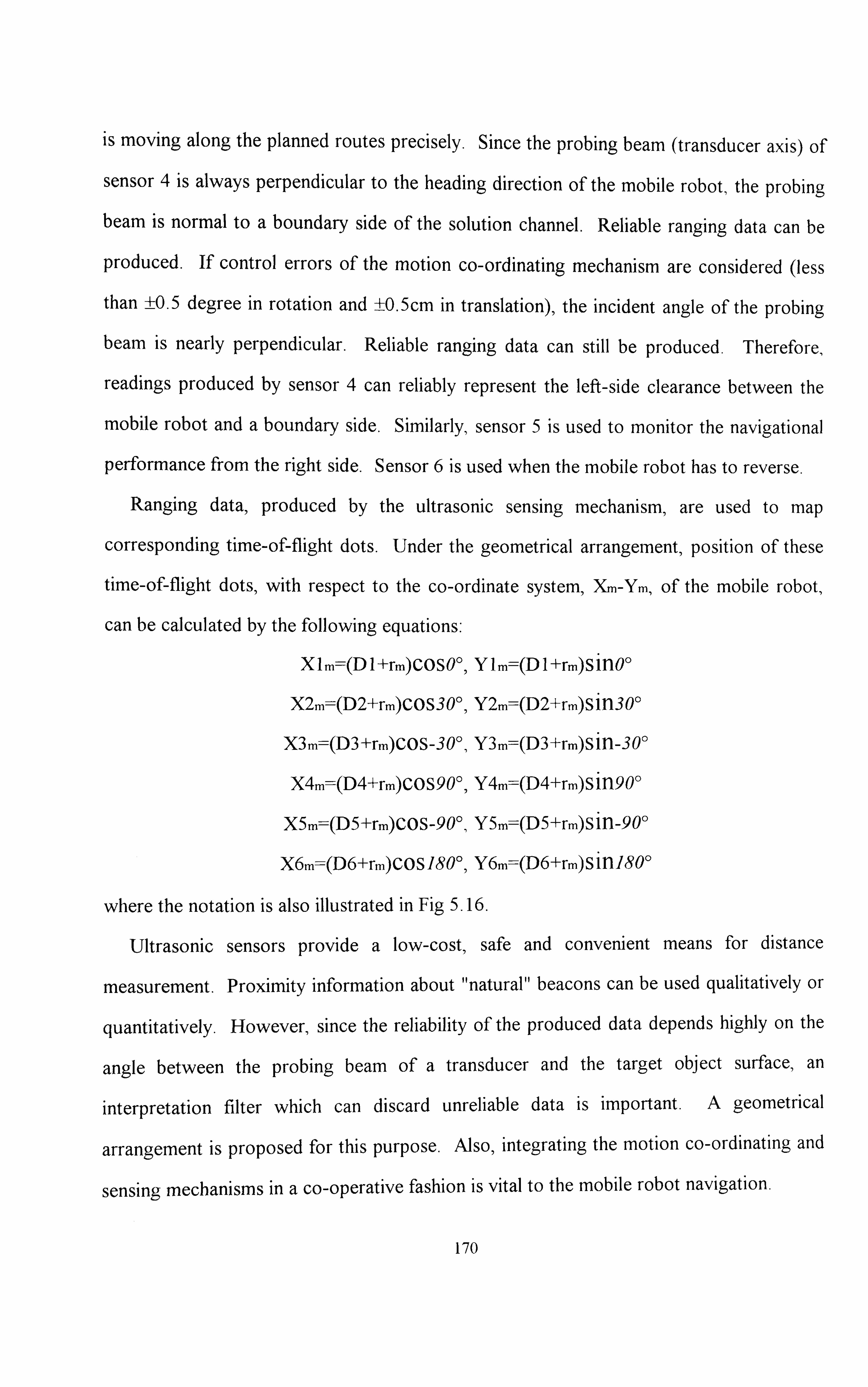
is moving along the planned routes precisely, Since the probing beam (transducer axis) of
sensor 4 is always perpendicular to the heading direction of the mobile robot, the probing beam is normal to a boundary side of the solution channel. Reliable ranging data can be
produced. If control errors of the motion co-ordinating mechanism are considered (less
than ±0.5 degree in rotation and ±0.5cm in translation), the incident angle of the probing beam is nearly perpendicular. Reliable ranging data can still be produced. Therefore,
readings produced by sensor 4 can reliably represent the left-side clearance between the
mobile robot and a boundary side. Similarly, sensor 5 is used to monitor the navigational
performance from the right side. Sensor 6 is used when the mobile robot has to reverse.
Ranging data, produced by the ultrasonic sensing mechanism, are used to map
corresponding time-of-flight dots. Under the geometrical arrangement, position of these
time-of-flight dots, with respect to the co-ordinate system, YM-Ym, of the mobile robot,
can be calculated by the following equations-
Xlm=(Dl+rm)COSOO, YIM
X2m=(D2+rm)COS30', Y2m
X3m=(D3+rm)COS-30', Y3m
X4m=(D4+rm)COS90', Y4m
X5m=(D5+rm)cos-900, Y5m
X6m=(D6+rm)COS]800, Y6m
(D I +rm) Sinoo
(D2+rm)Sin3O'
(D3+rm)Sin-30'
(D4+rm)Singoo
(D5+rm)Sin-goo
(D6+rm)Sini8oo
where the notation is also illustrated in Fig 5.16.
Ultrasonic sensors provide a low-cost, safe and convenient means for distance
measurement. Proximity information about "natural" beacons can be used qualitatively or
quantitatively. However, since the reliability of the produced data depends highly on the
angle between the probing beam of a transducer and the target object surface, an
interpretation filter which can discard unreliable data is important. A geometrical
arrangement is proposed for this purpose. Also, integrating the motion co-ordinating and
sensing mechanisms in a co-operative fashion is vital to the mobile robot navigation.
170

5.5. IMPLEMENTATION
This section describes the implementation of the triangulation based planning approach to the mobile robot. The target is to embody the mobile robot with an executing
capability, which can manage the motion co-ordinating and sensing mechanisms to achieve the proposed discrete navigation, specified by a route and associated operation scheme of the mobile robot.
5.5.1. Mana2im! Mechanism
In order for the mobile robot to smoothly execute a navigation, co-operatively
integrating the navigation planning, motion co-ordinating and sensing mechanisms is
important [48]. Since the three mechanisms have been individually discussed and
developed, a managing mechanism is developed for the integration purpose. This
managing mechanism is functionally similar to the two used in the graphical user interface
tool and the manipulator simulation system, section 5.1 and 5.2, but operates a different
motion co-ordinating mechanism (mobile robot vs. computer screen vs. manipulative
robot) and sensors (optical encoders and ultrasonic sensors vs. human operator vs. vision
camera).
During navigation, the managing mechanism continuously receives on-line sensory
information, which comes from the ultrasonic sensing mechanism and the optical encoders
of the motion co-ordinating mechanism. As a result, the managing mechanism has to filter
and integrate the sensory information Figure 5.17 illustrates the implementation
structure.
171

I navigation planning mechanism I
user reference -4 managing mechanism --------------- motion co-ordinating mechanism
supervisor level controller
-------------------- --- - --- - ---------- Ic ommand level contro
motor level controller
--- --- ----------- motor dg riVin
sensor driving
signal interpreting
optical enc oders mobile robot
----------- -------- -------- ---------------
- ---------------------- -------- - --------------- -- ---------------- -- - ---------
-------------- - L sensing mechanism
supervisor level controller
command level contr oller
transducer level controller
sensor II signal driving interpreting
ultrasonic sensors ------------------------- ------
Figure 5.17. Managing mechanism
5.5.1.1. Management of Sensory Information
The acquisition of sensory information, by the motion co-ordinating mechanism
(optical encoders) or the sensing mechanism (ultrasonic transducers), is individually
interpreted. Each mechanism produces sensory information of a specific module. The
two information modules are both exported to the managing mechanism to construct a
common environmental representation in the co-ordinate system of the navigation planner.
Due to the intrinsic limitations of the qualitatively different sensing devices, it is essential
to integrate information coming from these sensors. Specific assertions provided by the
information modules are correlated to each other in the managing mechanism.
In general, sensory information can be used by a mobile robot for four purposes-
(1) obtaining a priori information about the environment for the initial planning [57],
(2) localisation by matching against the build-in or constructed map [49][149],
(3) correction of the position and orientation errors [50][150][15 1],
(4) detection of potential obstruction and miMmisation of the effects [47][51][152].
172
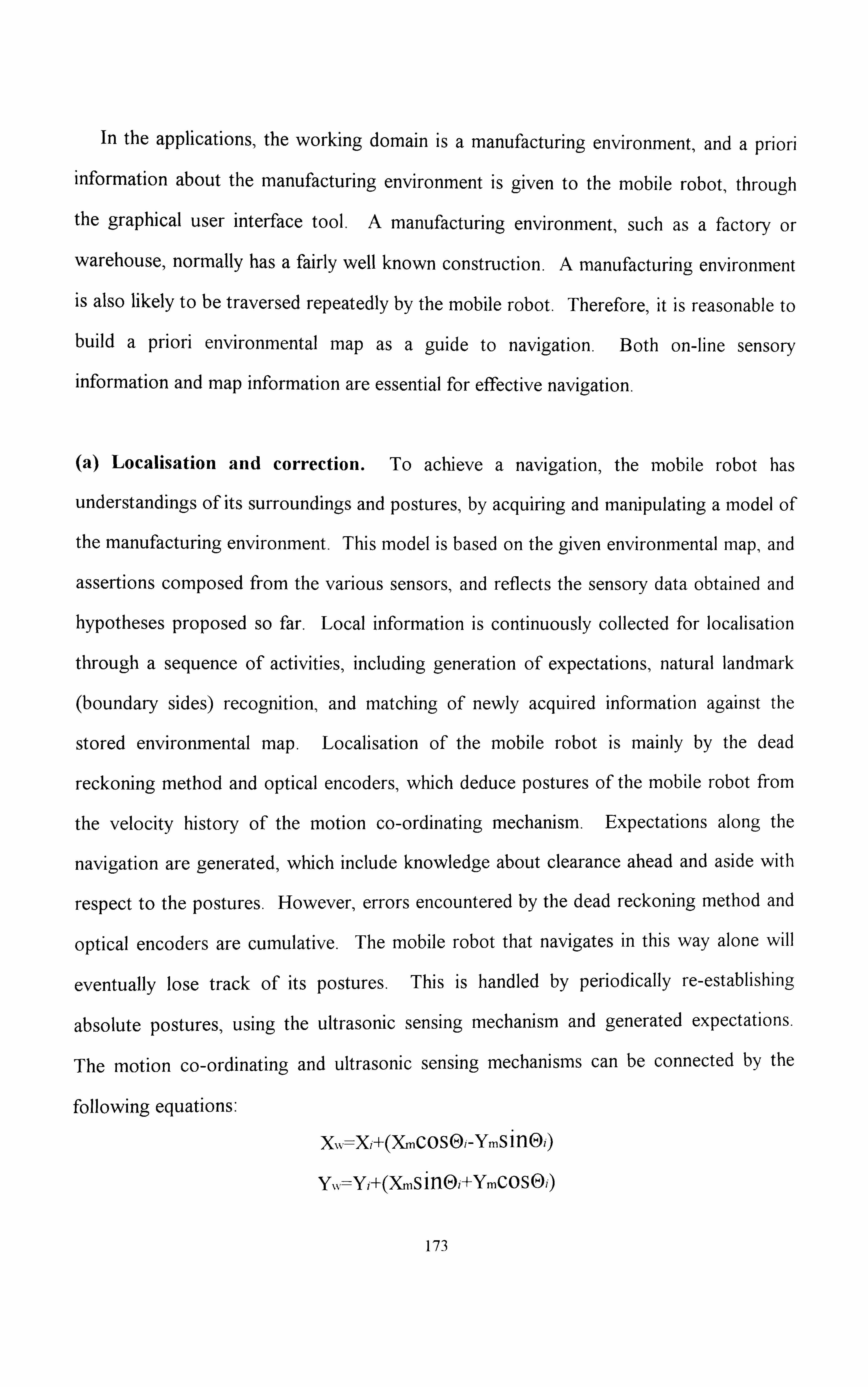
In the applications, the working domain is a manufacturing environment, and a priori
information about the manufacturing environment is given to the mobile robot, through
the graphical user interface tool. A manufacturing environment, such as a factory or
warehouse,, normally has a fairly well known construction. A manufacturing environment is also likely to be traversed repeatedly by the mobile robot. Therefore, it is reasonable to
build a priori environmental map as a guide to navigation. Both on-line sensory
information and map information are essential for effective navigation.
(a) Localisation and correction. To achieve a navigation, the mobile robot has
understandings of its surroundings and postures, by acquiring and manipulating a model of
the manufacturing environment. This model is based on the given environmental map, and
assertions composed from the various sensors, and reflects the sensory data obtained and
hypotheses proposed so far. Local information is continuously collected for localisation
through a sequence of activities, including generation of expectations, natural landmark
(boundary sides) recognition, and matching of newly acquired information against the
stored environmental map. Localisation of the mobile robot is mainly by the dead
reckoning method and optical encoders, which deduce postures of the mobile robot from
the velocity history of the motion co-ordinating mechanism. Expectations along the
navigation are generated, which include knowledge about clearance ahead and aside with
respect to the postures. However, errors encountered by the dead reckoning method and
optical encoders are cumulative. The mobile robot that navigates in this way alone will
eventually lose track of its postures. This is handled by periodically re-establishing
absolute postures, using the ultrasonic sensing mechanism and generated expectations.
The motion co-ordinating and ultrasonic sensing mechanisms can be connected by the
following equations:
X,, v: l--Xi+(Y... mcosOi-YmsinE)i)
Yýk, -----7: Yi+(XniSinoi+ymcosoi)
173

where (X, yi, R) is the posture of the mobile robot at the time instant ti, (ViNni) the
position of one of the six time-of-flight dots with respect to the mobile robot, and (Xvv, Y-w)
the position of the time of flight dot with respect to the co-ordinate system of the
manufacturing environment, Fig. 5.18(a).
Although the mobile robot can reliably navigate, an error in rotation can cause a
significant offset displacement after a long translation distance. The rotation error has
been experimentally showed to be small (less than ±0.5'), but happening often and
randomly. If posture (X,, Y,, Oi) is produced by the dead reckoning method and optical
encoders, section 5.3.1.2, the produced (Xw, Yw) position will be different to the expected
(Xw, Yw) position. Since a route segment of the planned discrete navigation is always
parallel to a boundary side (or nearly parallel if the rotation error is considered), the two
side ultrasonic sensors can reliably produce ranging information. By comparing the
ranging information with the expected distance, posture correction is made. Figure
5.18(b) illustrates the method.
Yw Ym Xm
0 4 Oi
Y, 06 3
0
. -xw
boundarv ýj ýý D4' D4 It
2 (C planned 4T 2 ()\ A t 1(ýrj executed ý6 16'
33)
S Xi
Ao= tan-' ((D4'-D4)/S) (a) (b)
Figure 5.18. Localisation and correction
(b) Obstacle detection. When the mobile robot is navigating, the ability to avoid
colliding with unexpected obstacles in the path is necessary and important. In order to
avoid objects, the mobile robot has to detect them first. In the implementation, the
ultrasonic sensing mechanism is also used for the detection of unexpected obstacles. An
174

obstacle is viewed as a solid object, which extends vertically from the ground surface to a
height more than the altitude of the sensor ring (about 30cm). Detection is defined as a
discontinuous state variation in one of the six ultrasonic sensors due to the acquisition of
sensed data relating to an obstacle. The front three sensors, 1,2 and 3, are mainly for
detecting unexpected obstacles ahead, acting as sensor bumpers. Since thresholds can be
assigned to the front three sensors, a safety strategy for the mobile robot is produced.
Figure 5.19 illustrates the safety strategy.
boundary (D2+r. )sln30>r,,,
irrevelant data D2>r..
clearance space 'ý"'-blind zone 4 2 2
............. ........................ route .................... 3
Dl> 2sin o
Dl> r n, (D3+r.. )sln30>r,, sin 0
D3>r. rn, -. radius of mobile robot
(a) (b)
Figure 5.19. Thresholds for clearance
r 2
rm Ideally, if a DI value, D1> -. ýý-90crn, is given to sensor 1, enough clearance space sino
for the mobile robot to pass through can be assured, Fig. 5.19(a). However, this strategy
is not practical for small or crowded environments, since the angular resolution of the
transducer, 20, is known to be low (20-250), and hence DI is large. Therefore, sensors 2
and 3 are used to assist sensor I in crowded environments, Fig. 5 . 19(b). A threshold
value greater than the radius of the mobile robot (rmýý15.5cm) is given to sensors 2 and 33,
D2, D3>rm, which confirms the clearance space. As a result, the threshold value, assigned
to D 1, can be reduced to D I> rim;: t45cm. A blind zone is an area which is not covered
2sinO
I- by any sensor beam. Although there are blind zones among the three sensor ranges, the
175

DI> riM- assignment can assure that an unexpected obstacle, which is within a blind 2sinO
zone of the clearance space, will be detected by sensor 2 or 3 before collision. Any discontinuous state variation of the two side sensors, 4 and 5, which is irrelevant to the
expectations for boundary edges , is ignored.
5.5.1.2. Management of Activities
The goal of the navigation strategy at the executing stage is to automatically compose
and perform suitable motor profiles for wheeling and steering, as well as to activate
sensors, according to the planned route and associated operation scheme. This stage
carries out the navigation plan that is exported to it, while adapting the motion co-
ordinating mechanism to real-world conditions as detected by the sensing mechanism. It
also provides an interface for user reference, through a function of the graphical user interface tool. Therefore, a successful collision free navigation is a result of the managing
mechanism co-operatively integrating the planning, sensing, and motion co-ordinating
mechanisms to move the mobile robot between two admissible postures.
The managing mechanism is responsible for the scheduling of activities of the
mechanisms, and for combining plan driven (actions) and sensory data driven (reactions)
activities in an integrated manner to achieve coherent behaviours. These activities are
mainly for two purposes- maintaining navigation and handling unexpected obstacles.
(a) Maintaining navigation. To achieve the prescribed discrete navigation, the motion
co-ordinating mechamsm is requested to provide a sequence of motor actions first. These
motor actions describe the performance of the mobile robot along the navigation. The
mobile robot is then initiated to perform the motor actions. During the performance, the
posture estimates for the mobile robot, with respect to the environmental map, are mainly
based on the velocity history of wheeling and steering, and subject to readings from the
176
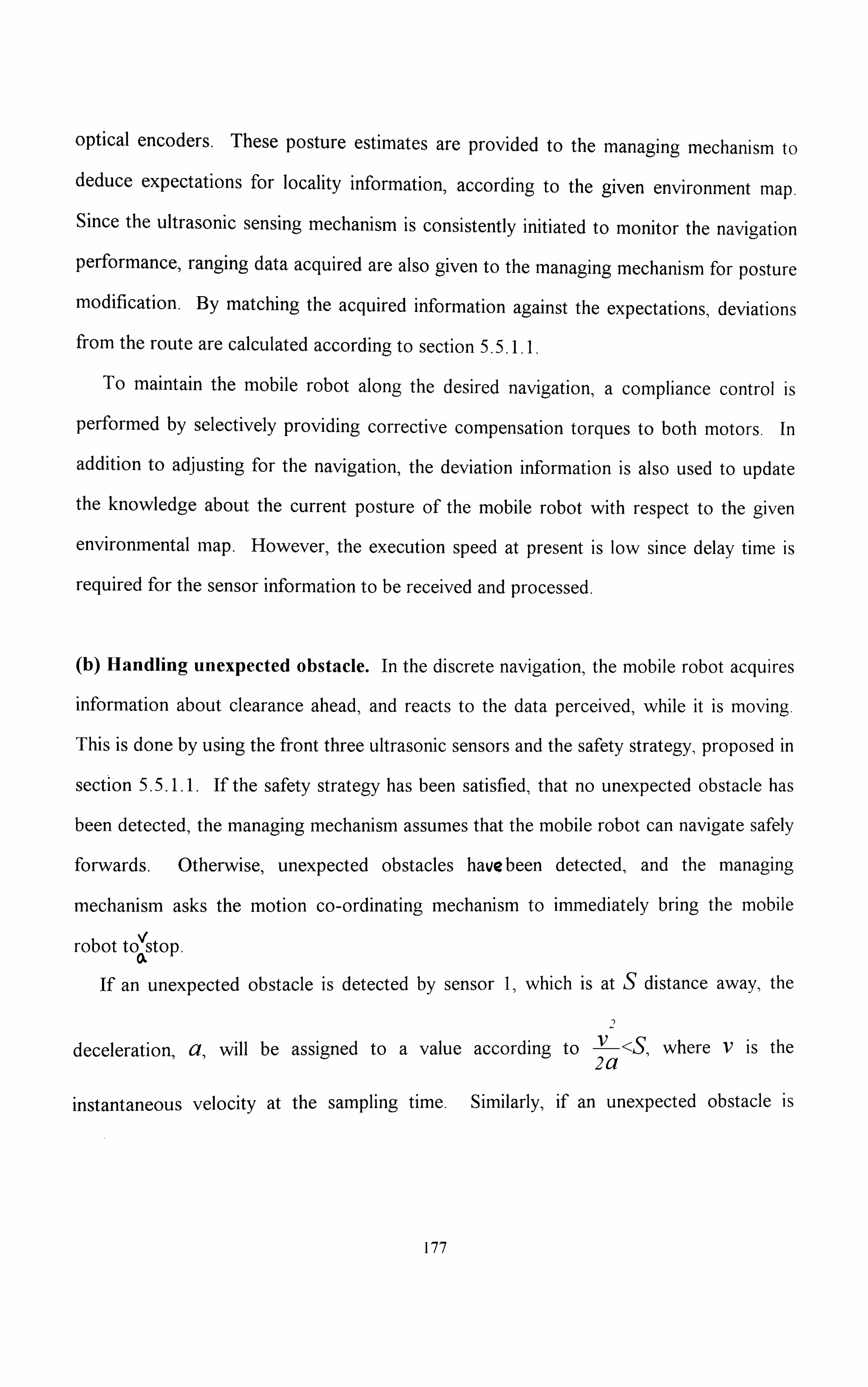
optical encoders. These posture estimates are provided to the managing mechanism to deduce expectations for locality information, according to the given environment map. Since the ultrasonic sensing mechanism is consistently initiated to monitor the navigation
performance, ranging data acquired are also given to the managing mechanism for posture
modification. By matching the acquired information against the expectations, deviations
from the route are calculated according to section 5.5.1.1.
To maintain the mobile robot along the desired navigation, a compliance control is
performed by selectively providing corrective compensation torques to both motors. In
addition to adjusting for the navigation, the deviation information is also used to update
the knowledge about the current posture of the mobile robot with respect to the given
environmental map. However, the execution speed at present is low since delay time is
required for the sensor information to be received and processed.
(b) Handling unexpected obstacle. In the discrete navigation, the mobIle robot acquires
information about clearance ahead, and reacts to the data perceived, while it is moving.
This is done by using the front three ultrasonic sensors and the safety strategy, proposed in
section 5.5.1.1. If the safety strategy has been satisfied, that no unexpected obstacle has
been detected, the managing mechanism assumes that the mobile robot can navigate safely
forwards. Otherwise, unexpected obstacles havebeen detected, and the managing
mechanism asks the motion co-ordinating mechanism to immediately bring the mobile
robot tAtop. 0. If an unexpected obstacle is detected by sensor 1, which is at S distance away, the
2
deceleration, a, will be assigned to a value according to -E-<S, where V is the 2a
instantaneous velocity at the sampling time Similarly, if an unexpected obstacle is
177

detected by sensor 2 or 3, which is at S distance away, the deceleration, a, will be
2 V-3 assigned to a value according to V <-S.
2a 2
Once the mobile robot stops, the managing mechanism will export the unexpected obstruction message and posture information to the planning mechanism to plan a diverted
or new navigation, and direct the navigation plan executing again.
5.5.2. Implementation Results
A general task for the flexible material transport system is to safely deliver materials from one location to another within a manufacturing environment. The mobile robot
navigation is fundamental. Presented is the implementation results of the triangulation
based navigation planning approach, using aB 12 three-wheel omni-directional mobile
robot and six Polaroid ultrasonic sensors.
To initiate a navigational task, a job description (goal posture) as well as an
environmental map (obstacle information) are given to the planning mechanism through
the graphical user interface tool. A discrete navigation is planned, which consists of a
route and associated operation schemes. This navigation plan is interpreted, by the motion
co-ordinating mechanism, to a sequence of motion commands of the mobile robot. The
sensing mechanism, operating a ring of ultrasonic sensors, produces surrounding
information for the detection of unexpected collisions and modification of navigational
behaviours. The managing mechanism routinely integrates the sensing and motion co-
ordinating mechanisms to monitor and correct the navigation performance, while the
mobile robot is carrying out the planned discrete navigation.
In the implementation, the ultrasonic sensing mechanism performs two functions. First,
it provides a means for safe encoder-based movement. Range readings from the three
forward sensors are subjected to the safety strategy, so that the mobile robot navigation is
sensitive only to unexpected obstacles located in the path. When an unexpected obstacle
178

is detected, the mobile robot brings itself to stop. The second function of the ultrasornc
sensing mechanism is to maintain clearance between the mobile robot and the
environmental boundary. Since the environmental map is given, clearance expectations
along the planned discrete navigation can be produced. By matching the ranging data
from the two side sensors against the produced expectations, posture errors can be
supplied to the motion co-ordinating mechanism, which then steers and drives the mobile
ro ot wit compensations.
S&G I
----- ------ low-
------------------ 78cm
planned clockwise route -01 ---------------- -- ------- -- -- ------- 156cm
position distribution
planned discrete navigation
Figure 5.20. Optical encoders only
179

Figure 5.20 illustrates experimental examples when the mobile robot is performing
navigation without integrating the ultrasonic sensing mechanism. A "point" obstacle is
assumed at the centre of the platform. Two discrete navigational tasks, requiring the
mobile robot to move along two square routes (78cm x 78cm and 156cm x 156cm) and
terminate at the start postures, are assigned. The terminating positions of the mobile robot
after several discrete navigational cycles are distributed as illustrated in the figure. Since
the motion repeatability of the mobile robot in this manufacturing environment has been
experimentally shown to be randomly within ±0.5cm and ±0.5 degree, the navigation
results can be analytically explained in Figure 5.21(a). From the start position, S, errors
are cumulative in turning at the four corners before reaching the goal position, G. Should
all the errors be positive and of maximum value then the total error, SG, for the case of the
156cm square route, can be estimated to be around I 1.2cm for a cycle run, Fig 5.21 (b).
s
planned practical
error one cycle GS
not to scale ----------------- -- ---- ------ -------- ------
(a)
78.5 156.5
S78 156 156
not to scale
78.5 G'
ii.
156 78 G
(b)
Figure 5.21. Error analysis
Similar to the implementation in Fig. 5.20, Fig. 5.22 illustrates experimental examples
when the ultrasonic sensing mechanism is invoked in the discrete navigation. Since the
ultrasonic sensing mechanism provides a function to maintain clearance between the
mobile robot and the environmental boundary, used for posture estimate and correction,
180

the lateral and longitudinal deviation is improved, compared with Fig. 5.20. The lateral deviation stops growing "out" after several runs of discrete navigation, which is subject to the reliability tolerance (5cm in the example) defined to the ultrasonic sensing mechanism. The longitudinal deviation also reduces since a compensation scheme (2.5cm for a cycle run) is applied.
S&G
all
--- -------- 78cm
planned clockwise route -- ------------- ------ ---------- 156cm
T
location distribution planned discrete navigation
Figure 5.22. Optical encoders 8-, ultrasonic sensors
Finally, Fig. 5.23 illustrates two discrete navigation experimental examples within a
layout of the manufacturing environment. In example 1, S1 to G1, the mobile robot
navigates to the goal without collision. In example 2, S2 to G2, an unexpected obstacle,
located in the path after the mobile robot starts the discrete navigation, is detected by one
181

(left-hand) of the three forward ultrasonic sensors (readings do not match the clearance expectations). The mobile robot then brings itself to stop.
example I example 2----- route to be contmued
Figure 5.23. Navigation examples
The ultrasonic sensors are not, at present, sufficiently developed to enable the extent of
the unexpected obstacle to be determined. When this is possible then from the stop
position further local triangulation might produce a safe navigation to the goal position
G2. Figure 5.24 illustrates the case.
182
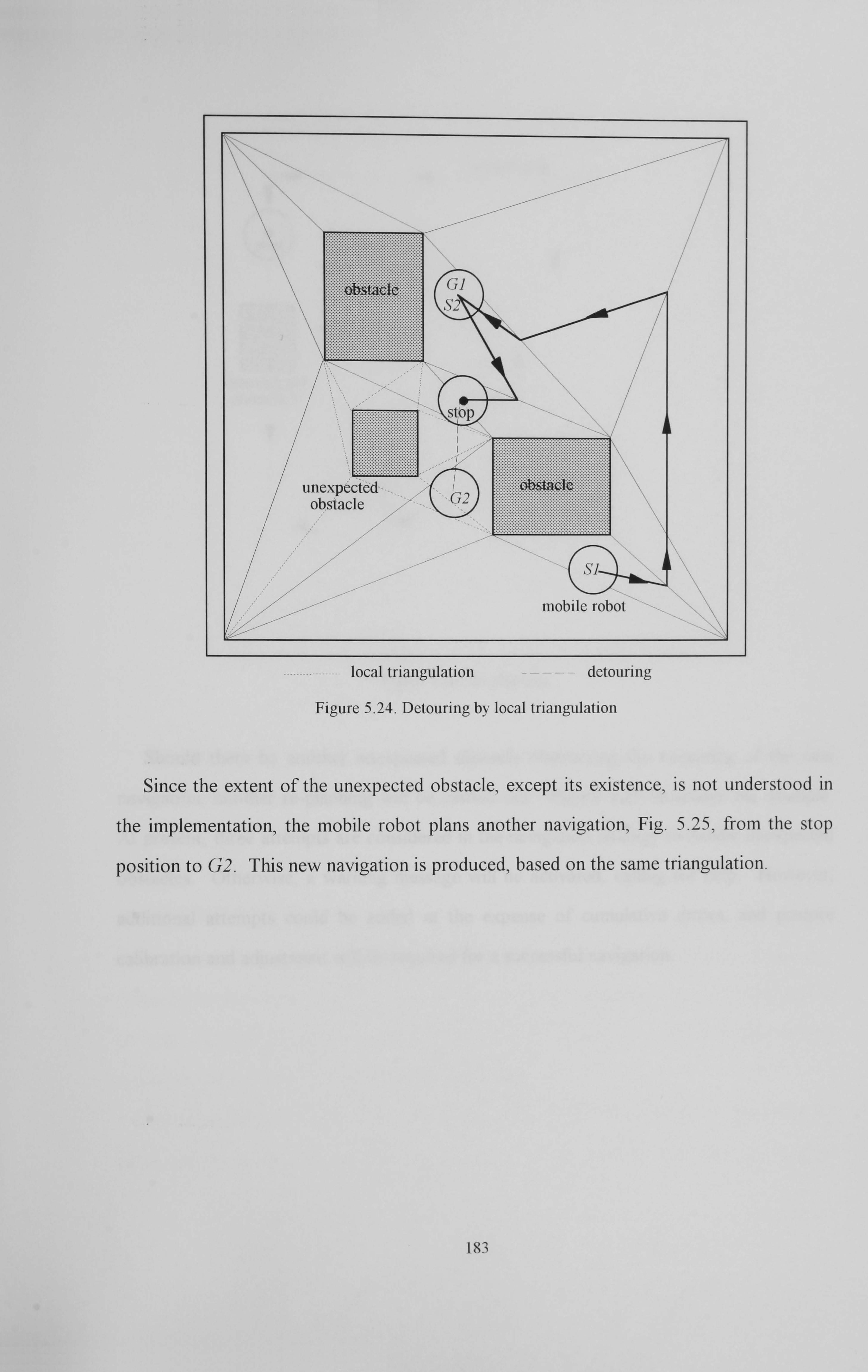
local triangulation detouring
Figure 5.24. Detouring by local triangulation
Since the extent of the unexpected obstacle, except its existence, is not understood in
the implementation, the mobile robot plans another navigation, Fig, 5.25, from the stop
position to G2. This new navigation is produced, based on the same triangulation.
183

Figure 5.25. Re-planning
Should there be another unexpected obstacle obstructing the executing of the new
navigation, another re-planning will be carried out. Figure 5.26 illustrates the example.
At present, three attempts are considered in the navigation strategy to handle unexpected
obstacles. Otherwise, a warning message will be activated, calling for help. However,
additional attempts could be added at the expense of cumulative errors, and posture
calibration and adjustment will be required for a successful navigation.
184

ON Do- gas ----
st p
..............
177777777777
77777
unexpected obstacle 2
..................... .................... ........... ............ ................... ........ .................. ..... ............ ....... - --- ....... ........ .......... ..........
. ......... unexpected obstacle I
...........
re-planning -04 - . --- -of
Figure 5.26. Re-planning
Thus the feasibility is shown of applying the triangulation based navigation planning
approach to a mobile robot within a manufacturing environment.
5.6. SUMMARY
At the executing stage, two motors of the mobile robot are co-operatively managed to
perform the planned navigation. The optical encoders and ultrasonic sensors are used to
provide navigation-related information. This information is necessary for making
decisions, performance corrections and further plans.
Posture estimates of the mobile robot along the navigation route are produced by the Z: )
dead reckoning method and optical encoders. These posture estimates are used to
185

generate surrounding expectations according to the given environmental map. These
surrounding expectations include information about the front and side clearance of the
mobile robot at the produced postures. Since the posture estimates by the dead reckoning
method and optical encoders are based on the kinematic history of the mobile robot, and
are thus prone to accumulated errors, making as regular as possible corrections is
necessary.
The correction method activates the ultrasonic sensors to obtain the clearance distances between the mobile robot and the surrounding obstacles. Although the
ultrasonic sensors also have uncertainties, each measurement is an independent event, directly interacting with an object. Therefore, the sensory errors are "absolute" but
"accumulated", and can be handled if a reliability tolerance is defined to the ultrasonic
sensing mechanism. By matching the obtained clearance distances against the surrounding
expectations, errors can be calculated, and unexpected obstacles can also be detected.
Compensations are then provided to adjust the mobile robot navigation.
The feasibility of the triangulation based navigation strategy has been verified by three
steps of practical implementation, using the computational graphical simulation,
manipulative robot, and mobile robot. Since the developed strategy does not use artificial
beacons or physical guidance, the navigational tasks the mobile robot can perform are
flexible. In other words, costs for re-initiating delivery tasks, given a new manufacturing
environment or production plan, are low.
186

CHAPTER SIX
DISCUSSIONS, CONCLUSIONS AND FUTURE DEVELOPMENT
Principal tasks of the flexible material transportation include delivering documents or
parts within a constructed (known) work place such as a warehouse, factory or office.
This constructed work place normally consists of stationary boundary walls (building
structure), and temporarily fixed but removable objects such as space partitions, working
benches and tooling machines. Once a new production plan is given, a new interior layout
of the work place, or a new manufacturing procedure, will be designed correspondingly.
The temporarily fixed but removable objects may consequently be re-located. The
delivery system has to be re-initiated as soon as possible for the new production plan. In
addition, the less system adjustment and associated modification costs the better.
At present, goods conveyors are widely used in industries for material transportation,
and floor-buried cable-guided vehicles are used in many instances. These systems have
advantages for mass production. However, due to their inherent physical constraints, it is
difficult to modify the delivery routes and re-irUtiate them for flexible production. They
are too rigid and restrictive to satisfy the required flexibility. Constructing a flexible
187

material transport system which contains functions for mobility, manipulation, perception
and automated control, and can deliver materials freely according to a given production
plan , is a desired solution to the problem. A mobile robot project, aiming at developing a
navigation strategy for a flexible material transportation system in a manufacturing
environment , is the accomplished objective of this work.
6.1. DISCUSSIONS
A flexible material transport system is constructed, consisting of off-the-shelf systems,
and software for communications and control. A navigation strategy is developed for the
mobility agent of the flexible material transport system, including triangulation based
planning and executing approaches. This navigation strategy produces collision-free
delivery in an efficient and flexible manner, and can handle unexpected obstacles and
emergencies.
6.1.1. Pro*ect Features
The ultimate goal of studying robotics is to produce universal human like behaviours.
As a contribution towards this, the mobile robot project is focused on the flexible material
transportation for factory automation. The purpose is to enable a mobile robot to navigate
itself freely, safely and efficiently from one location to another. Features of the mobile
robot project are.
(a) The mobile robot navigates in a manufacturing, indoor and constructed environment.
This feature makes it easier to model the working place, to attain surrounding information
and communications, and to plan navigation. The types of problems that may be
encountered are also constrained. However, the mobile robot may not continue its current
188

navigation due to unexpected obstacles. In these cases, the mobile robot reports failure,
or determines its location and then plans another navigation to achieve the destination.
(b) The mobile robot functions with minimum impact on the manufacturing environment.
That is, the mobile robot can navigate between the current inhabitants in the environment,
and avoid obstructions, without causing danger to itself, other machines, and buildings.
This also implies that the mobile robot is self-contained, and the manufacturing
environment is not equipped with external guidance mechanisms, such as embedded wires
(or painted stripes) in the floor or sensory beacons on the walls that can be followed. All
perceiving and guiding functions are performed by the on-board equipment.
(c) Efforts have been devoted to developing a system which can autonomously plan,
perceive, and co-ordinate actions. The mobile robot project has two functional parts,
hardware (the flexible material transport system) and software (the triangulation based
navigation strategy), together with four development principles:
(c. 1) modularity- integrating general-purpose off-the-shelf systems and devices-,
(c. 2) expandability. capable of adding components for future expansion,
(c. 3) flexibility: rapidly adjustable to different applications,
(c. 4) feasibility: applicable to practical scenes.
6.1.2. The Flexible Material Transport System
A working flexible material transport system, which consists of a mobile robot, an
articulated robot, ultrasonic sensors, a vision camera, and a personal computer, has been
constructed as a research test bed. Its hardware structure is principally divided into an
operational unit and a processing unit. To function, the system also needs on-board
power and input information.
189
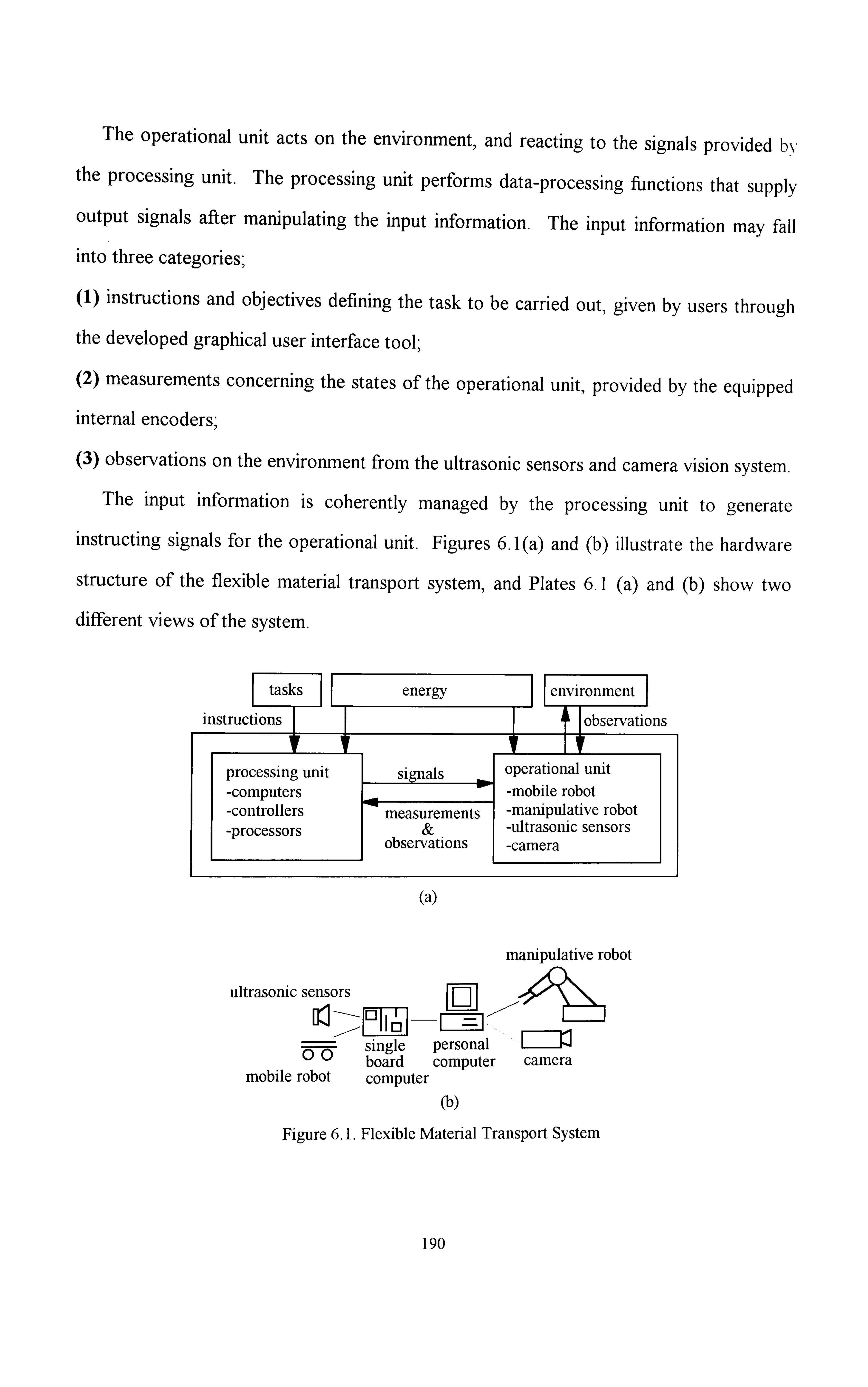
The operational unit acts on the environment, and reacting to the signals provided bN' the processing unit. The processing unit performs data-processing functions that supply output signals after manipulating the input information. The input information may fall into three categories,
(1) instructions and objectives defining the task to be carried out, given by users through the developed graphical user interface tool;
(2) measurements concerning the states of the operational unit, provided by the equipped
internal encoders;
(3) observations on the environment from the ultrasonic sensors and camera vision system. The input information is coherently managed by the processing unit to generate
instructing signals for the operational unit. Figures 6.1 (a) and (b) illustrate the hardware
structure of the flexible material transport system, and Plates 6.1 (a) and (b) show two
different views of the system.
energy environment I
instruc 41 observations
processing unit signals so operational unit
-computers . 09 -mobile robot -controllers measurements -manipulative robot -processors & -ultrasonic sensors
observations -camera
(a)
ultrasonic sensors
single 00 board mobile robot computer
manipulative robot
personal computer camera
(b)
Figure 6.1. Flexible Matenal Transport System
190

Plates 6.1 (a) & (b) The Flexible Material
IP 4
Transport System In % 'A
fI
-46
191

6.1.3. The Trianulation Based Navigation Strategy
A new navigation strategy for mobile robots in a manufacturing environment has been developed. This strategy works at two stages, planning and executing, and is based on triangulation approaches. The planning stage is to generate a collision-free navigational route. System behaviours are then co-ordinated, at the executing stage, to perform the
planned navigational route.
The planning stage of the navigation strategy is sequentially divided into a global
journey planning step and a local route planning step. The global 'ourney plannin(I step
carries out operations for spatial reasoning and graph mapping. AtFlangulated model of
the free space is employed to construct a triangulation graph. A node of the triangulation
graph represents a triangular partition of the free space, and an edge represents the
topological connectivity of two triangular partitions (nodes). Searching the triangulation
graph will produce a solution graph path. This solution graph path is actually a space
channel bounded by physical objects, which represents a global journey (trend) for a
mobile robot towards the given destination. A variety of navigational routes for the
mobile robot to follow are included in the solution space channel. The final navigational
route is then locally determined according to physical criteria, which contain cost
requirement, robot kinematic constraints, and unexpected obstruction.
The local route planning step only works on the space channel produced by the global
journey planning step. Since the space channel is a sub-set of the overall free space of the
mobile robot, searching efforts irrelevant to the final navigational route can be saved. In
addition, a navigational route planned by the triangulation based strategy is always within
the free space of the mobile robot, and, thus, collision free.
The executing stage of the navigation strategy is to manage operations of motion co-
ordinating and sensing. Since the final navigational route to be followed is designed to
keep clearance distances to obstacles and to be parallel to the- environment boundary,
ultrasonic sensors can be integrated to generate reliable observations for monitoring the
192

navigation. Executing programs for performing the planned navigational route in the
computational graphical simulation environment, or using the manipulative robot have also been developed.
The advantages of the navigation strategy are summarised as follows-
(a) Efficiency. The planning efficiency of a navigation strategy depends on the C65i; n
environment yeFyeseniatori and route searching approaches. For navigation strategies using
graphs, the efficiency is described by the computational complexity for constructing and
searching the graphs. Given a manufacturing environment with n vertices in total, the
developed navigation strategy takes O(ný running time to produce a triangulation graph
with O(n) nodes and O(n) edges. The visibility graph has O(n) nodes and O(n 2) edges,
and requires O(n 2) computation cost to form [73][114][119][123]. The Voronoi diagram
is another useful environmental representation, taking O(n 2) running time to construct,
and has a network of linear and parabolic line segments of 0(nlgn) data size [ 119][124].
The approximate cell decomposition produces connectivity graphs, with cell-resolution
dependent computation costs, but leads to loss of completeness [75][119][126].
Comparing with these existing approaches, the developed navigation strategy provides a
solution of similar efficiency.
(b) Simplicity. When planning a navigation, the larger and more complicat(Athe
manufacturing environment is, the more computational effort Is required. The global
journey planning stage works on the currently available environmental information to
produce a spatial channel (a journey), which merely indicates a preferable movement trend
of the mobile robot. Since the local route planning stage only concentrates on the
produced spatial channel, a much smaller space of interest rather than the whole
manufacturing environment is manipulated. A solution navigation is then locally planned
within the journey, subject to local criteria, and on-line knowledge update about the
193

neighbouring environment. As a result, calculations that are irrelevant to the solution
navigation are saved , in addition to the structural simplicity (small data size) of the triangulation graph.
(c) Clearance. Since the produced journey, or solution channel, is a subset of the free
space, it accommodates clearance distances to the environmental boundary. Due to this
clearance, the final navigation to be performed can be flexibly planned locally In the
journey according to the navigation mode, sensors equipped, and cost requirement. Once
a navigation is planned, it is adjustable to avoid unexpected obstacles through the
clearance space. The mobile robot performance can be monitored through using on-board
ultrasonic sensors to maintain the clearance space. Impact on the manufacturing
environment, caused by the executing uncertainties, can be decreased. In addition,
continuous navigations (curve routes) can be planned in the journey.
6.1.4. Experiments
The feasibility of the triangulation based navigation strategy has been demonstrated and
verified by three steps of practical implementation, using a computational graphical
simulation tool, a manipulative robot, and a mobile robot-
(a) A graphical simulation environment has been developed on a personal computer. It is
a useful and convement tool for a user to preview and exarmne the navigational
performance of the mobile robot in a possible interior layout, when designing or renewing
the manufacturing environment.
(b) A practical scene is imitated by incorporating a manipulative robot with a vision
camera system to draw the planned paths on a board, clustered with toy blocks. This
work enables a user to investigate the candidate environmental layout designed at the (a)
194

step, and to do fine adjustments before the candidate design is finally applied to the manufacturing environment.
(C) Implementation of the navigation strategy is completed by using a mobile robot with
ultrasonic sensors on board. As the developed triangulation based navigation strategy
always provides clearance space for uncertainty and error correction, collision-free
performance is produced by the mobile robot.
6.2. CONCLUSIONS
Presented in this thesis is the design and construction of a mobile robot system, which
is able to perform flexible material transportation tasks in a manufacturing environment. An attempt to actually implement a working system with imprecise control, capable of functioning in an environment with uncertainties, is also represented. Although the
difficulties of autonomous system operation are still not completely understood, the
research efforts have given some insight into what the problems really are.
This research project has produced a simple and flexible navigation strategy for mobile
robots working within a manufacturing environment, and has investigated the
implementation issues. Three major parts of the project are concluded as following:
(a) System. A fleXible material transport system with a centralised control structure has
been constructed for manufacturing applications. To be capable of autonomous
operations, this system requires functions for manipulation, mobility, perception, and
intelligence. Therefore, off-the-shelf systems, including a manipulative robot, a mobile
robot., ultrasonic sensors, a compass, a camera, a single board computer, and a personal
computer, are put together, as component systems, for the purpose. Since signals have to
be exchanged frequently and smoothly among these component systems, and different
195

systems have different interface configurations, cables and control programs for
communications are produced. To achieve the centralised control mode, the personal
computer is used to manage the other component systems. Since all intelligent processing tasks are performed by the personal computer, software which can drive and supervise the
component systems from the personal computer is also composed. Hence the flexible
material transport system is ready to be operated by the developed navigation strategy.
(b) Navigation strategy. A common feature for mobile robots and navigation problems
is that uncertainties and errors exist, which accumulate along with the working time.
Therefore, clearance spaces for navigation to tolerate control, modelling, and operational
uncertainties, and sensors and sensing methods to detect errors and unexpected obstacles
are two required features for a working strategy to accomplish a safe navigation. A new
triangulation based navigation strategy has been developed for mobile robots to perform
navigational tasks for flexible material transportation. Given a mobile robot and a
manufacturing environment, this strategy can plan a feasible and collision-free navigation,
and direct the mobile robot to safely execute the navigation. The strategy also has
functions anticipating various contingencies, and can survive with limited sensing ability.
At the planning stage of the strategy, triangulation approaches are used to model the free
space of the environment as a graph. Since triangles are easy to handle, a graph model of
this feature has a simple structure, and is easy to manipulate. The solution navigation
planned by searching on the graph is safe and collision free, because clearance spaces for
uncertainty tolerance are considered. Handlers for unexpected obstacles are also
developed to use the clearance spaces. In addition, searching efficiency is provided due to
the simplicity of the graph structure. At the executing stage of the strategy, the two
motors of the mobile mechanism are co-operatively managed to perform the planned
navigation. The optical encoders and ultrasonic sensors are used to provide on-line
navigation-related information, which is necessary for decision making, performance
196

correcting, and further planning. Posture estimates of the mobile robot, and thus the
surrounding expectations, along the navigation are produced. By matching the
surrounding expectations against the clearance distances between the mobile robot and the
surrounding obstacles, obtained by the ultrasonic sensors, errors as well as unexpected
obstacles can be detected. Compensations are then provided to adjust the mobile robot
navigation. Since the developed strategy does not use artificial beacons or external
equipment for guidance, the navigational tasks the mobile robot can perform are flexible.
(c) Implementation. Practical implementations and demonstrations have been conducted
to verify the feasibility of the developed navigation strategy, using a computational
graphical simulation, a manipulative robot with camera, and a mobile robot with six
ultrasonic sensors as tools. In the computational simulation, users can input and renew
information of a manufacturing environment, and communicate with the flexible material
transport system, through the developed graphical user interface tool. The planning
operations of the strategy as well as the solution navigation can be illustrated on a
computer screen. The implementation using a manipulative robot with camera is to set up
a quick-responding and small-scaled simulation system. Information about the working
environment,, produced by a camera, is given to the navigation strategy. A solution
path is planned, which is then plotted on a board by a manipulative robot. This
implementation shows that the developed navigation strategy works well with an
automatic information provider, the camera. In the implementation using a mobile robot
and six ultrasonic sensors, uncertainties have been recognised as an important factor to the
navigation safety. Optimality is only meaningful when collisions and damages can be
avoided. The implementation shows that the solution navigation planned by the developed
strategy is error tolerant due to the clearance feature. In addition, the navigation strategý',
based on the ultrasonic sensors working on the clearance feature, can effectively reduce
the errors.
197

The thesis describes contributions to an on-going mobile robot project. The system is not yet a perfectly integrated autonomous system, and does not perform all the tasks that its hardware is designed and integrated to do. However, significant progress has been
made given the time and monetary constraints. Further developments are issued.
6.3. FUTURE DEVELOPMENT
The developed mobile robot system, thougý t is able to perform autonomous navigation,
rt is confined to the flexible material transportation in a manufacturing environment.
Therefore, future research efforts will be focused on improving the system towards stand-
alone ions. .
and extending the system applicability to other applicati
6.3.1. System Improvement
One of the ultimate goals of robotics is to create an autonomous system that can
perform tasks independently for hours without outside assistance. Such an unattended
autonomous system will accept and execute high-level descriptions of tasks without
further human intervention. In general, an autonomous system needs four principle
functions; mobility, manipulation, perception, and intelligence. Since the constructed
flexible material transport system is a working system, already consisting of component
systems for the four functions, the hardware improvement will be carried out in two ways'.
(a) System integration. Currently the manipulative robot and the vision camera system
of the flexible material transport system are installed aside a docking site. A mobile robot
system having an onboard manipulator to acquire and retrieve objects will be an economic
solution to loading and unloading materials instead of setting systems for every docking
sites. In addition, equipping the vision camera system on the mobile robot to make it
198

capable of visual tracking and visual detectio'n will be helpful for controlling system behaviours. Therefore, the first step of improvement will be to integrate the present
component systems into a compact form. Then, the module functions for manipulation,
perception, and intelligence will be available on the mobility platform to achieve moblie robot operations autonomously.
(b) Advanced Perception. After the system integration, the mobile robot system will have optical encoders, ultrasonic sensors, and a vision camera on board for assessing
tasks, environment and related interface interactions. Different types of sensory information will have to be handled.
(b. 1) The raw data obtained by the three different types of sensors have to be processed
by the corresponding pattern recognition functions before use. A considerable amount of
work will have to be done, such as in [153], to make these sensing functions more reliable
and efficient.
(b. 2) Equipping the mobile robot system with more sensors implies that more information
about the environment can be obtained, and sensory data fusion is important. Sensory
data fusion approaches filtering conflict or superfluous information will be investigated.
(b. 3) Independently building maps of the real world for navigation planning may not be
necessary at present, since the environmental maps are provided by users. However, a
representation of the environment autonomously determinable in a period of time by the
mobile robot system, capable of being integrated into the navigation, will increase the
safety, as suggested in [154]. Much work will have to be done to develop techniques to
construct environmental maps from the raw sensory data.
(b. 4) A low-cost and reliable self-localisation strategy is the key to many unsolved
problems in mobile robotics. Once a map building function is available, investigations into
a feasible and robust self-localisation method will be carried out.
199

6.3.2. Further Applications
A flexible material transport system and a working navigation strategy for its mobile
robot have been developed to handle material delivery in a manufacturing environment.
Further implementations will be to employ the developed system to other applications.
(a) Continuous navigation. It seems to be more natural for a mobile robot system to
perform continuous navigation than discrete navigation. This research subject is attracting
attentions in the mobile robotics community. When directing a mobile robot system to
perform continuous navigation, three physical factors, the driving capability, the steering
capability and the centre of gravity of the mobile robot system, will have to be intensively
considered. These considerations will be vital to maintain navigation stability. Since the
developed navigation strategy preserves clearance spaces to the environmental boundary,
continuous navigation can be planned using the clearance advantage.
(b) Moving obstacles. In the basic application, all obstacles are assumed to be fixed.
Also,, there is only one mobile robot, made of a rigid object, navigating in the
manufacturing environment. However, the navigation problem can easily be made
complicate in dynamic environments. One extension of the problem consists of including
moving obstacles in the environment. Another one allows multiple mobile robots to
operate within the same environment; each being a potential obstacle to others. Since
unexpected obstacle handlers have been proposed, efforts will focus on extending the
unexpected obstacle handlers to these problems.
200

LIST OF PUBLICATIONS
Parts of the research project have been presented and published in the following
conferences and associated proceedings. The present work has benefited by helpful
feedback and comments from other researchers in this field.
(1) The International Conference on Automation, Robotics, and Computer Vision,
ICARCV92, Singapore, September 1992- Implementation of Robot Collision-Free Path
Planning in a Maze Using the Triangulation Algorithm,
(2) The IEEE International Workshop on Emerging Technologies and Factory
Automation, EFTA'92, Australia, August 1992. An Algorithm for Robot Path Planning
with Obstacle Avoidance Using Triangulated Model,
(3) The IEEE/RSJ International Conference on Intelligent Robotics and Systems - Intelligent Robots for Flexibility, IROS'93, Japan, July 1993 Japan- Space Representation
and Map Building -a Triangulation Model to Path Planning with Obstacle Avoidance,
(4) The International Conference on Advanced Mechatronics - Great Advancement of
Intelligent Machines, ICAM'93, Japan, August 1993 - Implementation of the Triangulation
Algorithm to Robot Path Planning Problem;
(5) The ASME European Joint Conference on Engineering Systems Design and Analysis,
ESDA'94, United Kingdom, July 1994- Extended Triangulation Algorithm for Robot Path
Planning with Obstacle Avoidance.
201

APPENDIX A
MOVEMASTER-EX MANIPULATIVE ROBOT
The MOVEMASTER-EX manipulative robot, manufactured by Mitsubishi company, is
a vertical articulated link structure comprising five revolute joints. Physically, it has 19kgf
of weight, up to 1.2kgf of lift capacity, and 1000mm/sec of maximum path velocity
measuring at the wrist tool surface [39] Nomenclature of this manipulative robot is
illustrated in Fig. A. 1.
A. l. Mechanism
The manýipulative robot has five DC electrical servo motors which are powered from an
ordinary 240-voltage electrical socket through an internal adapter in the control unit.
Motors for J I, J2 and B produce 30W of output, motors for J4 and J5 yield I IW, and
there are relay cards handling in/out signals from the control unit to motor circuitry [39].
The upper arm and fore arm are rigid with 250mm and 160mm of length respectively. All
five joint movements are rotary. Joints JI and J5 are directly driven by motors, while
timing belts are used to transmit mechanical power to joints J2, B and J4, from the
corresponding motors. Limit switches and brakes are equipped to define the work
envelop of the manipulative robot. The end effector is a DC servo motor driven gripper
202

with two rigid fingers. Its opening/closing stroke range is from Omm to 60mm. This
600gf weighted gripper has a grip capability of up to 3.5kgf [39]. Table A. I is a brief
summary of the robot specifications.
Joint Limit Brake Timing Belt Specifications (from Origin Switch reference configuration)
ii Yes No Direct Drive ±150' (max. 120'/sec) J2 Yes Yes Yes +100', -30' (max. 72'/sec) J3 Yes Yes Yes -110' (max. 1090/sec) J4 Yes No Yes ±90' (max. 100'/sec) J5 Yes No Direct Drive ±1800 (max. 1630/sec)
Table A. I Specifications of MOVENIASTER-EX
J3
(Wrist roll) J5 Joint 5
J4
Gripper
T-I-+ A/N JVIIIL -r
(Wrist pitch)\ Joint 2 (Shoulder)
Wrist tool surface (Gripper installation surface)
J2
Joint I (Waist)
Power & signal cables 171
Zý- to control system Base
Figure A. 1. (a) Robot articulation [3 91
Side view
Figure A. L(b) Reference configuration (Origin) 139]
Fore arm
\
Joint 3 (Elbow)
Upper arm
203
Top vicNN I

A. 2. Control Unit
The MOVENIASTER-EX manipulative robot has a dedicated control computer, the Drive Unit, functioning as power adapter, motor amplifier, motion controller and monitor,
and signal input/output interface, to support the robot's mechanism.
A motor pulse encoder system, instead of hardware (optical) encoders, is equipped for
position detection and motion control of the robot mechanism. In addition to ROM
memory accommodating the operational system, battery-backed static RAMs are used for
data storage, - 629 positions and 2048 program steps can be recorded for programming
[39]. Also, there is a built-in EPROM writer for EPROM recording. The input/output
module of the Drive Unit supports one parallel interface (Centronics standard), one serial
interface (EIA-RS232C standard), one teaching box input port and one motor signal
output port for interface with peripheral systems and the robot mechanism. The
emergency stop action can be initiated by pressing the emergency button on the Drive
Unit,, or on the teaching box.
As to the operational software, the Drive Unit uses the PTP (Point-To-Point) position
control approach, with the linear interpolation on the articulated movements to manage
joint motions, enabling the robot mechanism to move in either articulated or Cartesian
patterns [39]. The Drive Unit can be programmed through the teaching box (NIDI,
Manual Data Input) or an external computer. The lead-through programming, using the
teaching box, can be accomplished by playing back recorded positions and operational
processes. The operational software has a set of programming languages with BASIC-like
structure and syntax. Using these 63 commands, designed to control five joints and one
additional axis (gripper), off-line programm-ing can be achieved from an external
computer, via the serial/parallel interface. All parameters required by the commands can
be directly entered in the form of millimetre or degree [39]. Ten steps of speed, up to
"' 9 1000mm/sec of path velocity at the wrist tool surface, can be set to run the robot [)
204

APPENDIX B
B12 MOBILE ROBOT
The mobile robot used is aB 12 mobile robot manufactured by Real World Interface
Inc. It is a cylindrical, three-wheeled and self-contained platform with motors, power
amplifiers, batteries, optical encoders, microprocessor-based control boards, and
supporting operational software. Dimensionally, the mobile robot is 17.15cm (6.75
inches) in height and 30.48cm (12 inches) in diameter [191. It is structurally rigid with an
aluminium frame, and 11.3 5 kgf (25 pounds) in total weight [ 19].
B. I. Mechanism
The mobile robot has two DC motors, each independently functioning as the
translation (driving) actuator and the rotation (steering) actuator. Both motors provide
1.13Nm of torque enabling the mobile robot to carry loads of up to 20kgf [ 19]. Four on-
board re-chargeable lead-acid batteries, providing 144 watt hours of electrical power, are
also able to support additional devices, such as computers and sensors, with 12-voltage
power through the 24-pin connector on the top surface of the mobile robot [ 19].
The mobile robot has a three-wheeled synchronous mobile mechanism. Through the
specially designed transmission apparatus, the translation motor and the rotation motor
can independently drive and steer the mobile robot. The three wheels remain parallel at all
205

times, even during the steering. The parts of the mobile robot that interact with the ground are three identical wheels whose treads are made of moulded polyurethane [ 19].
They are pivoted with rigid suspensions to the robot's body frame, measuring 4.15cm
radii. For measuring movement, the mobile robot has two incremental optical shaft
encoders mounted on the shafts of the motors. Each optical shaft encoders provides 500
counts per motor revolution [ 19].
The three-wheeled driving and three-wheeled steering mechanism gives the mobile
robot stable traction and an omni-directional moving capability. Figure B. I illustrates the
driving mechanism.
.......... ........... ... ......... - .... ............ ........... .......... ...... .............. ............... ....... ................ ........ ................. ....... .................. .......... ..... ...... .......... .......
........... ........... ..... .............. .... ...... ............ ................... .................. ....... ................... ............ . .... ................... ............
...................... ................................. ............ .................. ................................. ............... ... . .................. ............. ................. ......... ................. ....... ................. ............... ...... ......... ..... ...... ................ ..... ................ .... ..................... .... ...................... .... ..................... ... .......... ..................... .................... .............. ........... ....... ................... ................... .................. .................. .................. ................ ...........
................ ................ ................ ................. ...............
w heading direction
Figure B. 1. Synchronous mobile mechanism offering omm -directional movement
B. 2. Control Unit
The control unit of the mobile robot has six control boards including power amplifier
module, encoder module, central processing module, memory module and input/output
module. The control unit also monitors electrical current levels of the batteries and
motors. This current-monitoring function can be used as a kind of bumper sensor. A set
of motion/position control commands are provided by the manufacturer for off-line
programming.
206

(a) Circuitry. The power amplifier module has two similar pulse-width modulator boards. Each board contains servo amplifier and current monitoring cIrcuitr-y, and manages the servo-drive current to one motor. The encoder module is accomplished b\,
two encoder drive boards. Each shaft encoder has its own drive board to inanage
operations, and produces feedback counting signals. Since both encoder drive boards zero their counters in every system reset,, the angular positions of the motors can be
cumulatively measured from the reset moment. Motor velocity and acceleration are derived by constantly checking the first and second differentiation of the angular position (position and velocity changes over a stable time base) respectively.
The central processing and memory modules are carried out by two boards built
around a NEC78310 rnicroprocessor with 32k bytes of ROM and 32k bytes of RAM.
Operational software and instructions are stored in ROM, and user programs of up to
32768 8-bit words, or approximately 550 commands, can be stored in the RAM [ 19]. The
input/output module facilitates the system interface in two modes-
(a-1) Human user. The present control level is displayed by the indicating LEDs on the
front panel. In case of non-recoverable errors, error messages will be illuminated on the
'Status' LED using the international Morse codes. An exclusive input port accepting
signals from a remote emergency switch has the first interruption priority. Pressing the
emergency switch will disconnect both translation and rotation motors to the batteries, and
also immobilise the mobile robot with brakes.
(a. 2) Serial communications. The mobile robot interfaces with external systems only
through its serial communications port with 4kb receive buffer, 2kb transmit buffer, and
two connectors. This serial communications port is partially compatible with the EIA-
RS232C standard, but has a different configuration in that it does not provide the
handshaking signals for Data Carrier Detect, Data Terminal Ready, Data Set Ready. and
Clear To Send. The two connectors are logically wired in parallel, and will cause data
207

collisions if they are used simultaneously. The 9-pin sub-miniature D connector is on the
front panel, and the 24-pin double row 0.1 -inch connector is on the top surface of the
mobile robot.
(b) Operational software. The motion/position control commands use two alphabetic
mnemonic characters, and can be classified as status and action commands. A status
command either returns an internal status of the mobile robot, such as elapsed time,
present motor angular position, battery condition, or assigns a velocity or acceleration
value to the mobile robot. An action command causes the mobile robot to move, limp or
halt. Each of the translation and the rotation servo loops can be independently operated in
velo . city, position, power or limp modes. Parameters responding to or required by control
commands are in hexadecimal notations, and extra conversion programs are necessary to
translate the particular parameters into meaningful values (metre, second, etc. ) for user
debugging and programming. The default value is zero if no parameter is entered after a
command.
208

APPENDIX C
COMPUTERS
In the design of the flexible material transport system, all calculations of intelligent I- activities,, such as supervising, decision making, planning, modelling, scheduling, module
co-ordinating, monitoring, exception handling, are carried out by a host personal
computer. A single board computer is equipped on the mobile robot to deal with general
operations on the remote moving platform. This single board computer connects the
control units of the mobile robot and the ultrasonic sensor system through a passive back
plane (a system bus board).
C. I. Host Computer
The host computer, from ELONEX Inc., is based on a standard architecture designed
by IBM Inc. The mother board has an Intel 803 86SX- I 6Mhz microprocessor and I N1B of
random access memory. The adapter for the visual display unit supports a VGA colour
monitor. The use of the VGA monitor provides an animation environment for the
developed graphical user interface tool with resolutions of 640 by 480. As to system
interface and external signal transmission, the personal computer has two serial
communications Ports, with 9-pin sub-miniature D connectors, supportIng the EIA-
RS232C configurations [71][72]. It also has one parallel communications port with a -'ý-
209

pin sub-miniature D connector (EEC-625, International Electrotechnical Commission),
supporting the IEEE-488 GPIB (General Purpose Interface Bus) configurations [155][156]. Operational software running on this personal computer is the MS-DOS
(Nficrosoft Disk Operating System) and the Nlicrosoft VaNDOWS.
C-2. Sin2le Board Computer
The applied single board computer is a Gespac MPL-4080 single board computer [66],
manufactured by MPL AG Elektronikunternehmen and based on a Motorola 68HCOOO-
8NfRz microprocessor. This single board computer has 1024 bits of EEPROM allowing
the storage of useful operating parameters [66]. The 512kb RAM is backed up by an on-
board lithium battery [66]. For input/output extension, the single board computer
supports two programmable serial ports and a G-64 bus interface. At the software level, a
low-level software tool, Xbug [ 157], is contained in the monitor ROM for developing and
debugging programs. At present, the single board computer is installed on the mobile
robot for instructing ultrasonic perception and mobility performance through the G-64 bus
interface.
C. 3. Miscellaneous
A GESBUS-8M bus board, manufactured by GESPAC S. A. [158], is used to connect
the control board of the ultrasonic sensors and the interface board of the mobIle robot
with the N4PL-4080 single board computer. This bus board supports the G-64 bus
configuration, and has eight slots accepting Euroboard expansion cards [26]. It caters for
8-bit or 16-bit processors (sixteen individual data lines are provided), and permits
asynchronous as well as synchronous data transfer [26]. The eight expansion slots apply
the DIN41612 form-C 96-pin connectors.
A DC to DC adapter is included to supply the bus board and other accessories with
volt power at 8 amps. Power to this adapter is provided by the batteries on the mobile
210

robot through the 24-pin connector and the mobile robot interface board. The mobile
robot interface board, also supporting the G-64 configuration, is plugged into the
GESBUS-8M bus board to manage power from the mobile robot and organise serial
communications with other systems.
211

REFERENCES
11] Robotics and Automated Manufacturing; Richard C. Dorf, Reston Publishing Company Inc. 1983 [2] Economic Indicators; The Economist 1993,1994,1995, The Economist Publications [31 Fortune International 1993,1994,1995; TIME Inc. [41 RIA Robotics Glossary; Robotic Industries Association [5] Robotics and Automated Manufacturing; D. Sharon, J. Harstein, G. Yantian; World ORT Union. Pitman Publishing 1987 [6] Robotics: Introduction, Programming, and Projects; James L. Fuller; Macmillan Publishing Company 1991 [71 Fundamentals of Industrial Robots and Robotics; Rex Miller, PWS-KENT Publishing Company 1988 [81 Industrial robotics; Bernard Hodges; Butterworth-Heinemann Newnes Ltd. 1992 [9] Robotics and Automated Systems; Robert L. Hoekstra; South-Western Publishing Co. 1986 [ 10] Assembly with Robots; Tony Owen; Kogan Page Ltd. 1985 [I I] Fundamentals of Robot Technology; D. J. Todd; Kogan Page Ltd. 1986 112] A Supervisory System for Free Ranging Automated Guided Vehicles; Chung-Shing Wang. PhD Thesis 1991, Imperial College, University of London [ 13 ]A Free Ranging AGV; G. Drunk; International Journal of Machine Tools and Manufacture. Volunie 28, Number 3,1988, Page 263-272 [14] Fundamentals of Robotics Engineering; Harry H. Poole; Van Nostrand Reinhold Co. Ltd. 1989 [ 151 Mobile Robots: Inspiration to Implementation; Joseph L. Jones, Anita M. FIN-nn. A. K. Peters Ltd. 1993 [ 16] Robotics Japan: New Technology Japan, Special Edition 1991 & Robotics Japan: Robot Technologý - Past, Present and Future; Machinery and Technology Department; Japan External Trade Organisation (JETRO) 1991 117] Robotics in Service; Joseph F. Engelberger; Kogan Page Ltd. 1989 [ 181 A Mobile Automaton: An Application of Artificial Intelligence Techniques. Niles J. Nilsson-. Proceedings of the International Joint Conference on Artificial Intelligence, U. S. A. 1969 [ 191 B 12 Operational Manual; Real World Interface Inc. [20] Popular Science 1992,1993,1994,1995, Times Mirror Magazines, Inc. [2 1] Robot Technology-Modelling and Control, Volume L, Phillippe Coiffet; Kogan Page Ltd. 1983 [22] Computer and Interfacing: Connection to the Real World; Martin Cripps, Edward Arno d Inc- & Hodder & Stoughton Ltd. 1989 [23] Microcomputers and Their Interfacing; R. C. Holland; Pergamon Press Ltd. 1984 [24] Computers and Microprocessors-Components and Systems-, A. C. Downton; Van Nostrand Reinhold (UK) Co. Ltd. 1988 [25] Microprocessor Systems: Interfacing and Applications; Robert J. Bibbero, David M_ Stern-' John Wiley and Sons Inc. 1982 [26] Bus-Based Industrial Process Control; Michael Tooley; Heinemann Newnes Ltd. 1988 [27] The RS-232 Solution-How to Use Your Serial Port; Joe Campbell. SYBEX Inc. 1989 [28] Robots and Telechirs; M. W. Thring; Ellis Horwood Ltd. 1983
1 [29] Intelligent Robotics Control; George N. Saridis; IEEE Transactions on Automatic Control. Volume AC-28, Number 8, August 1983, Page 547-557 [30] Computing Techniques for Robots; Igor Aleksander-, Kogan Page Ltd. 1985 [3 1] Robot Rover Visual Navigation; Hans P. Moravec-, University Microfilms International Research Press 1980 [32] A New Method of Vehicle Position Measurement by Using Laser Beam Tracking-. T. Tsurnura. N.
Fujiwara, M. Hashimoto, T. Tang; Advanced Robotics, Volume 2, Number 2,1987, Page 12 1- I') ý
133] Directed Sonar Sensing for Mobile Robot Navigation; John J. Leonard, Hugh F. Durrant-WhNle*.
Kluwer Academic Publishers 1992 1 Simple Maps of an Indoor Environment, Karen Beth [341 Visual Navigation: Constructing and Utilizing
Sarachik (Master Thesis, March 1989). Al-TR 1113, Technical Report 1113, Artificial Intellu4crice
Laboratory, Massachusettes Institute of Technology
212

[351 MARVEL: A System for Recognising World Locations with Stereo Vision; David J. Braunegg (PhD Thesis, June 1990); AI-TR 1229, Technical Report 1229, Artificial Intelligence Laboraton-. Massachusettes Institute of Technology 136] Robot Builder's Bonanza: 99 Inexpensive Robotics Projects; Gordon McComb. TAB Books, McGraw-Hill Inc. 1987 [37] A Colony Architecture for an Artificial Creature; Jonathan Connell (PhD Thesis, August 1989). Al- TR 115 1, Technical Report 15 5 1, Artificial Intelligence Laboratory, Massachusettes I nstitute of Technology [38] Error Detection and Recovery for Robot Motion Planning with Uncertainty; Bruce Randall Donald (PhD Thesis, June 1987); Al-fR 982, Technical Report 982, Artificial Intelligence Laboraton-. Massachusettes Institute of Technology [3 9] MOVEMASTER-EX Instruction Manual: Industrial Nficro-robot System Model RV-M I MITSUBISHI Co., Ltd. [40] Making Complex Machinery Move: Automatic Programming and Motion Planning, David A. Sanders; Research Studies Press Ltd. 1993 [4 11 PUMA Instruction Manual; Stdubli Unimation Inc. [421 Efficient Kinematic Transformations for the PUMA 560 Robot; S. Elgazzar; IEEE Journal of Robotics and Automation, 1985 September, Volume RA- 1, Number 3, Page 142-151 [431 Coordination of Action and Perception in a Surveillance Robot. James L. Crowley. IEEE Expert. Winter, 1987, Page 32-43 [44] An Efficient Algorithm for One-Step Planar Compliant Motion Planning with Uncertainty: Aiuy J. Briggs; Algorithmica, Volume 8, Number 3,1992, Page 195-208 [45] Robust Compliant Motion for Manipulators, Part 1: The Fundamental Concepts of Compliant Motion; H. Kazerooni, T. B. Sheridan, P. K. Houpt; IEEE Journal of Robotics and Automation. Volume RA-2, Number 2, June 1986, Page 83-92 [46] Animal Sonar Systems; R. G. Busnel, J. F. Fish; Plenum Press 1980 [47] A Bat-like Sonar System for Obstacle Localisation, Billur Barshan, Roman Kuc. IEEE Transactions on Systems, Man, And Cybernetics, Volume 22, Number 4. July/August 1992, Page 636-646 [48] Incorporating Range Sensing in the Robot Navigation Functions; Vladimir Lumelsky, Tim Skewis; IEEE Transactions on Systems, Man, and Cybernetics, Volume 20, Number 5, September/October 1990, Page 1058-1069 [49] Sensor-Based Self-localisation for Wheeled Mobile Robot, A. Curran, K. J. Kyrikopoulos'. Proceedings of 1993 IEEE Internal Conference on Robotics and Automation, U. S. A.. Page 8-13 150] Sonar-Based Real-World Mapping and Navigation, Alberto Elfes, IEEE Journal of Robotics and Automation, Volume RA-3, Number 3, June 1987, Page 249-265 [5 1] Obstacle Avoidance with Ultrasonic Sensors; J. Borenstein, Y. Koren; IEEE Journal of Robotics and Automation, Volume 4. Number 2, April 1988, Page 213-217 [52] A Kalman Filter Approach to Sensor-Based Robot Control; D. G. Johnson, J. J. Hill, IEEE Journal of Robotics and Automation, Volume RA-1, Number 3, September 1985. Page 159-162 1531 Laserrader and Sonar Based World Modelling and Motion Control for Fast Obstacle Avoidance of the Autonomous Mobile Robot MOBOT-11", Markus Buchberger, Klaus-Werner J6rg, Ewald von Puttkamer: Proceedings of 1993 IEEE International Conference on Robotics and Automation, May 2-6, 1993, U. S. A., Page 534-540 [54] Ultrasonic Sensing for Mobile Robot to Recognise an Envirorurnent-Measuring the Normal Line of Walls; Y. Nagashima, S. Yuta; IROS'92 Proceedings of the 1992 IEEE/RSJ International Conference on Intelligent Robots and Systems, July 7-10,1992, U. S. A., Page 805-812 155] Ultrasonic Sensor Information Sheets*, Polaroid Inc. [56] Tri-aural Perception on a Mobile Robot; H. Peremans, J. Van Campenhout, Proceedings of 1993
IEEE International Conference on Robotics and Automation, May 2-6.1993. U. S. A., Page 265-270
[571 Map Building for a Mobile Robot from Sensory Data; Minoru Asada. IEEE Transactions on Sý'stems.
Man, and Cybernetics, Volume 20, Number 6, November/December 1990, Page I) 1 26-1336
[58] Mobile Robot Localisation Using Sonar. Michael Drumheller, IEEE Transactions on Pattern
Analysis and Machine Intelligence, Volume pAMI-9, Number 2, March 1987. Page 325-3,2
213

[59] Sonarbased Outdoor Vehicle Navigation and Collision Avoidance; D. Langer, C. Thorpe: IROS'92 Proceedings of the 1992 lEEE/RSJ International Conference on Intelligent Robots and Systems. JuIv 7- 10. 1992, U. S. A., Page 1445-1450 [60] Toward Autonomous Driving: The CMU Navlab Part I-Perception; Charles Thorpe, Martial Hebert. Takeo Kanade, Steven Shafer; IEEE Expert, August 1991 [6 1]A Camera Space Control System for an Automated Forklift-, R. K. Miller, D. G. Stewart. H. Brockman, S. B. Skaar; IEEE Transactions on Robotics and Automation, Volume 10, Number 5. October 1994, Page 710-716 [621 MARVEL: A System that Recognises World Locations with Stereo Vision-, David J. Braunegg. IEEE Transactions on Robotics and Automation, Volume 9, Number 3, June 1993, Page 303-308 [631 Vision Camera Operational Manual; Data Translation Inc. 164] Structured Control for Autonomous Robots; Reid G. Simmons; IEEE Transactions on Robotics and Automation, Volume 10, Number 1, February 1994, Page 34-43 [65] A Control Architecture for an Advanced Fault-Tolerant Robot System; Andreas Hormann. Wolfgang Meir, Jan Schloen; Robotics and Autonomous Systems, 7(1991), Page 211-225 [66] WL-4080 Computer Information Sheet; MPL AG Elektronikunternehmen [67] Running Visual Basic for Windows: a Hands-On Introduction to Programming for Windows-, Ross P. Nelson; Microsoft Press 1993 [68] GW-BASIC Operating System User's Guide and Reference; Microsoft Corporation 1987 [69] Microsoft Quick BASIC: programmer's quick reference; Kris A. Jamsa; Microsoft Press 1989 [701 Absolute Beginner's Guide to Programming; Greg Perry, Sams Publishing Ltd. 1993 171] Complete Guide to RS232 and Parallel Connections- A Step-by-step Approach to Connecting Computers, Printers, Terminals, and Modems; Martin D. Seyer; Prentice-Hall Inc. 1988 [72] RS-232 Made Easy: Connecting Computers, Printers, Terminals, and Modems-, Martin D. Seycr', Prentice-Hall Ins. 1991 [73] Path Planning for Mobile Robot; Christos Alexopoulos, Paul M. Griffin; IEEE Transactions on Systems, Man, and Cybernetics, Volume 22, Number 2, March/April 1992, Page 318-322 [74] Shortest Paths for Line Segments; Christian Icking, Ganter Rote, Emo Welzi, Chee Yap'. Algorithn-iica, Volume 10, Number 2/3/4, August/September/October 1993, Page 182-200 [75] Shortest Path Planning in Discretized Workspaces Using Dominance Relation, Sungtaeg Jun, Kang G. Shin-, IEEE Transactions on Robotics and Automation, Volume 7, Number 3. June 199 1, Page 342-3 -50 [76] Continuous Steering-Function Control of Robot Carts-, Winston L. Nelson. IEEE Transactions on Industrial Electronics, Volume 36, Number 3, August 1989, Page 330-337 [771 Blanche-An Experiment in Guidance and Navigation of an Autonomous Robot; Ingermar J. Cox1 IEEE Transactions on Robotics and Automation, Volume 7, Number 2, April 1991, Page 193-204 [78] A New Family of Oninidirectional and Holonomic Wheeled Platform for Mobile Robot; Franois G. Pin, Stephen M. Killough-. IEEE Transactions on Robotics and Automation, Volume 10, Number 4. August 1994, Page 480-489 [79] A Motion Planning for Nonholononiic Mobile RoboC Jean-Paul Launiond, Paul E. Jacobs. Michel Taix, Richard M. Murray; IEEE Transactions on Robotics and Automation, Volume 10, Number 5. October 1994, Page 577-593 [801 A Robust Layered Control System for a Mobile Robot; Rodney A. Brooks-, IEEE Journal of Robotics
and Automation; Volume RA-2, Number 1, March 1986, Page 14-23 [811 Robot Motion Planning: A Distributed Representation Approach-, Jerome Barraquandý Jean-Claud Latombe; The International Journal of Robotics Research, Volume 10, Number 6, December 199 1, Pagc
51-72 [821 Algorithmic: The Spirit of Computing; David Harel; Addison-Weslev Publishing Company 1987
[83 ] Introduction to Algorithms; Thomas H. Cormen, Charles E. Leiserson, Ronald L. RiN esc The
Massachusetts Institute of Technology Press 1990 [84] Algorithms and Automatic Computing Machinesý B. A. Trakhtenbrot (translated and adapted from
Russian by Jerome Kristian, James D. McCawley)-, D. C. Heath Inc. 1963
[85] Computational Geometry-An Introduction, Franco P. Preparata. Michael Ian Shamos: Springer-
Verlag New York Inc. 1985
214

[861 Computational Geometry-A Survey; D. T. Lee. Franco P. Preparata; IEEE Transactions on Computers, Volume C-33, Number 12, December 1984, Page 1072-1101 [87] Introduction to Graph Theory; Robin James Wilson; Longman Group Ltd. 1979 [88] Euclidean Geometry and Convexity; Bussell V. Benson; McGraw-Hill New York Inc. 1966 [89] Elementary Topology: A Combinatorial and Algebraic Approach; Donald W. Blackett: Academic Press Ltd. 1982 [90] Convex Figures and Polyhedra; L. A. Liusternik (translated from Russian by T. Jefferson Smith). Dover Publication Inc. New York 1963 [9 1] From Geometry to Topology; H. Graham Flegg; The English Universities Press Ltd. 1974 1921 Decomposing a polygon into its convex parts; B. Chazelle, D. Dobkin; Proceedings of the II th Symposium on Theory of Computing (Atlanta, Ga, U. S. A., April 30-May 2). ACM New York 1979. Page 38-48 [93] Algorithms and Complexity; Herbert S. Wilf Prentice-Hall London Ltd. 1986 [941 Computer Algorithms: Introduction to Design and Analysis; Sara Baase; Addison-Wesley Inc. 1988 [95] Decomposing A Polygon into Simpler Components; J. Mark Keil; SIAM Journal on Computing. Volume 14, Number 4, November 1985, Page 799-817 [96] Convex Decomposition of Simple Polygons; S. B. Tor, A. E. Middleditch, ACM Transactions on Graphics, Volume 3, Number 4, October 1984, Page 244-265 [97] Decomposition of Polygons into Convex Sets-, Bruce Schachter; IEEE Transactions on Computers. Volume C-27, Number 11, November 1978, Page 1078-1082 [98] On Decomposing Polygons into Uniformly Monotone Parts; Robin Liu, Simeon Ntafos. Information Processing Letters, 27(1988) Page 85-89,29 February 1988 [99] An O(logn) Time Parallel Algorithm for Triangulating a Set of Points in the Plane, Cao An Wang, Yung H. Tsin; Information Processing Letters, 25(1987) Page 55-60,20 April 1987 [1001 New Results for the Minimum Weight Triangulation Problem; L. S. Heath, S. V. Pemmaraju. Algorithmica, Volume 12, Number 6,1994, Page 533-552 [101] Triangulation and Shape-Complexity; Bernard Chazelle, Janet Incerpi; ACM Transactions on Graphics, Volume 3, Number 2, April 1984, Page 135-152 [102] A Linear Time Algorithm for Triangulating a Point-Visible Polygon; T. C. Woo, S. Y. Shin, ACM Transactions on Graphics, Volume 4, Number 1, January 1985, Page 60-70 [ 103 ] Optimal Search in Planar Subdivisions; D. G. Kirkpatrick-, SIAM Journal on Computing, Volume 12, Number 1, February 1983, Page 28-35 [ 104] Triangulating Simple Polygons and Equivalent Problems, Alain Fournier, Delfin Y. Montuno, ACM Transactions on Graphics, Volume 3, Number 2, April 1984, Page 153-174 [105] Triangulating a Simple Polygon; Michael R. Garey, David S, Johnson, Franco P. Preparata, Robert E. Tarjan; Information Processing Letters, Volume 7 Number 4, Page 175-179, June 1978 [1061 An O(nloglogn)-Time Algorithm for Triangulating A Simple polygon-, Robert E. Tarjan, Christopher J. VanWyk; SIAM Journal on Computing, Volume 1.7, Number 1, February 1988, Page 143- 178 [107] An Efficient Algorithm for Decomposing a Polygon into Star-Shaped Polygons. D. Avis. G. T. Toussaint; Pattern Recognition, Volume 13, Number 6,1981, Page 395-398 11081 A Simple and Fast Incremental Randomized Algorithm for Computing Trapezoidal Decompositions
and for Triangulating Polygons; Raimund Seidel-, Computational Geometry: Theory and Applications, 1(1991), Page 51-64 [ 109] Convex Decomposition of Polyhedra and Robustness; Chandeijit L. Bajaj, Tamal K. Dcy: SIAM Journal on Computing, Volume 21. Number 2. April 1992. Page 339-364 [I 10] A Triangulation Algorithm from Arbitrary Shaped Multiple Planar Contours; A. B. Ekoule, F. C.
Peyrin, C. L. Odet; ACM Transactions on Graphics. Volume 10, Number 2, April 199 1. Page 182-199
[I III Shading of Regionson Vector Displav Devices; D. T. Lee, ACM Computer Graphics Volume 15.
Number 3, July 1981, Page 34-44 Feature Generation for Svntactic Pattern [1121 Decomposition of Polygons into Simpler Components.
Recognition; Hou-Yuan F. Feng, Theodosios Pavlidis; IEEE Transactions on Computers. Volume C-24.
Number 6, June 1975, Page 636-650
15

1113] A Survey of Motion Planning and Related Geometric Algorithms; J. T. Schwartz, M. Sharir: Artificial Intelligence, 37(1988), Page 157-169 [ 114] An Algorithm for Planning Collision-Free Paths Among Polyhedral Obstacles; Tomas Lozano- Perez, Michael A. Wesley; Communications of the ACM, Volume 22, Number 10. October 1979, Page 560-570 [115 ] Spatial Planning: A Configuration Space Approach-, Tomas Lozano-Perez; IEEE Transactions on Computers, Volume C-32, Number 2, February 1983, Page 108-120 [1 t6j A Subdivision Algorithm in Configuration Space for Findpath with Rotation; Rodney A. Brooks. Tomas Lozano-Perez; IEEE Transactions on Systems, Man, and Cybernetics, Volume SMC- 15. Number 2, March/April 1985, Page 224-233 1117] A Novel Representation for Planning 3-D Collision-Free Paths; Susan Bonner, Robert B. Kelley. IEEE Transactions on Systems, Man, and Cybernetics, Volume 20, Number 6, November/December 1990, Page 1337-1351 [ 118] Solving the Find-Path Problem by Good Representation of Free Space, Rodney A. Brooks. - IEEE Transactions on Systems, Man, and Cybernetics, Volume SMC-13, Number 3, March/April 1983, Page 190-197 119] Robot Motion Planning; Jean-Claude Latombe; Kluwer Academic Publishers 1993 120] Graphs and Their Uses; Oystein Ore; Random House 1963
[121] Principles of Artificial Intelligence; Nils J. Nilsson; Springer-Verlag Inc. 1982 [122] Finding the Shortest Route Using Cases, Knowledge, and Dijkstra's Algorithm-, Bing Liu, SicN%, - Hwee Choo, Shee-Ling Lok, Sing-Meng Leong, Soo-Chee Lee, Foong-Ping Poon, Hwee-Har Tan. IEEE Expert, October 1994, Page 7-11 [ 123 ] Computation of the Tangent Graph of Polygonal Obstacles by Moving-Line Processing*, Yun-Hui Liu; Suguru Arimoto; IEEE Transactions on Robotics and Automation, December 1994, Volume 10, Number 6, Page 823-830 [124] Motion Planning in a Plane Using Generalised Voronoi Diagrams; Osamu Takahashi. R. J. Schilling; IEEE Transactions on Robotics and Automation, Volume 5, Number 2, April 1989, Page 143- 150 [125] Motion Planning for an Autonomous Vehicle, Proceedings of the IEEE International Conference on Robotics and Automation, Page 529-533 1126] Navigation of a Car-Like Mobile Robot Using a Decomposition of the Environment in Conv
i ex
Cells; Hubert A. Vasseur, Franqois G. Pin, Jack R. Taylor; Proceedings of the 1991 IEEE International Conference on Robotics and Automation, Page 1496-1502 [ 127] A Potential Field Approach to Path Planning; Yong K. Hwang, Narendra Ahuja; IEEE Transactions on Robotics and Automation, Volume 8, Number 1, February 1992, Page 23-32 [128] Real-Time Robot Motion Planning Using Rasterizing Computer Graphics Hardware-, Jed Lengyle, Mark Reichert, Bruce R. Donald, Donald P. Greenberg; Computer Graphics, Volume 24, Number 4, August 1990, P327-335 [129] On the "Piano Movers"' Problem 1. The Case of a Two-Dimensional Rigid Polygonal BodN'Movlng Arnidst Polygonal Barriers; Jacob T. Schwartz, Micha Sharir, Communications on Pure and Applied Mathematics, VolumeXXXVI, P345-398 (1983) [130] Simulation and Animation of Sensor-Driven Robots; ChuXin Chen, Mohan M. Trivedi, Clint R. Bidlack; IEEE Transactions on Robotics and Automation, Volume 10, Number 5, October 1994. Page 684-704 [ 13 1] Introduction to the Special Section on Perception-Based Real-World Navigation; Bir Bhanu. Olivier Faugeras, Banavar Sridhar, Charles E. Thorpe; IEEE Transactions on Robotics and Automation. Volume 10, Number 6, December 1994, Page 725-727 [132] Navigation Templates: Mediating Qualitative Guidance and Quantitative Control in Mobile Robots-. Marc G. Slack; IEEE Transactions on Systems, Man, and CN-bernetics, Volume 23, Number 2, March/April 1993, Page 452-466 1133] An Integrated Architecture for Robot Motion Planning and Control in the Presence of Obstacles
with Unknown Trajectories-ý R. Spence, S. Hutchinson, IEEE Transactions on SN, steiiis. Man. and Cybernetics, Volumn 25, Number 1. January 1995. Page 100-110
'? 16

[ 134] Computer Graphics: An Introduction to the Mathematics and Geomet -- chae E. Mo enson: Heinemann Newnes Ltd. 1989 n Mi I rt 1135] An Obstacle Avoidance Algorithm for an Autonomous Land Vehicle; T. S. Chang, K. Q1u, J. J. Nitao; International Journal of Robotics and Automation, Volume 2. Number 1,1987. Page 21 25 [136] Exception Handling in Robotics; Ingemar J. Cox, Narain H. Gehani; Computer, March 1989, Page 43-49 [ 13 7] Optimal Polygonal Approximation of Digitized Curves; Y Zhu, L. D. Seneviratne, S. W. E. Earles: International Workshop on Image Analysis and Synthesis, Graz, Austria, June 1993 [138] An object-oriented Language for Constructing Simulations; David McArthur, Herm, Sowlzral. 7th International Joint Conference on Artificial Intelligence, IJCAI-81,24-28 August 198 1, University of British Columbia, Vancouver, B. C. Canada, Page 800-809 11391 A Beacon Navigation Method for Autonomous Vehicles-, Clare D. McGillem, Theodore S. Rappaport; IEEE Transactions on Vehicular Technology, Volume 38, Number 3, August 1989, Page 132- 139 [140] The Polaroid Ultrasonic Ranging System; C. Biber, S. Ellin, E. Sheck, J. Stempeck, 67th Audio Engineering Society Convention, New York, October 1980; Reprinted in Polaroid Ultrasonic Ranging System handbook [ 14 1] The Sonar Ring: Obstacle Detection for a Mobile Robot; Scott A. Walter-, Proceedings of the 1987 IEEE International Conference on Robotics and Automation, Page 1574-1579 1142] Ultrasonic Range Finders; Polaroid Corporation, Cambridge, MA, 1982 [ 143 ] G96 Sonar Board Guide to Operations, version 1.1, Real World Interface. Inc. [144] Physically Based Simulation Model for Acoustic Sensor Robot Navigation, Roman Kuc, M. W. Siegel; IEEE Transactions on Pattern Analysis and Machine Intelligence, Volume PAMI-9, Number 6, November 1987, Page 766-778 [ 145] Differentiating Sonar Reflections from Corners and Planes by Employing an Intelligent Sensor-, Billur Barshan, Roman Kuc; IEEE Transactions on Pattern Analysis and Machine Intelligence, Volume 12, Number 6, June 1990, Page 560-569 [146] A Spatial Sampling Criterion for Sonar Obstacle Detection; Roman Kuc; IEEE Transactions on Pattern Analysis and Machine Intelligence, Volume 12, Number 7. July 1990, Page 686-690 [147] Ultrasonics; B. Carlin, McGraw Hill New York Inc. 1960 [ 1481 Sonar Localisation for Mobile Robots: A Model-Based Approach; Bill Trigge, Stephen Cameron; IEEE International Workshop on Emerging Technologies and Factory Auto mation-Technol ogY for the Intelligent Factory, ETFA'92, August 11-14,1992, Melbourne, Australia, Page 387-392 149] Optimal Estimation of Position and Heading for Mobile Robots Using Ultrasonic Beacons and
Dead-reckoning; Lindsay Kleeman; Proceedings of the 1992 IEEE International Conference on Robotics and Automation, Page 2582-2587 1150] A Physically Based Navigation Strategy for Sonar-Guided Vehicles; Roman Kuc, Victor Brian Viard; The International Journal of Robotics Research, Volume 10, Number 2, April 1991. Page 75-87 [ 15 11 ROBNAV: A Range-Based Robot Navigation and Obstacle AN, oidance Algorithm; David F. Cahn. Stephen R. Phillips; IEEE Transactions on Systems, Man, and Cybernetics, September 1975, Page 544- 551 [1521 Feature Extraction Techniques for Recognising Solid Objects with an Ultrasonic Sensou. M. K. Brown, IEEE Journal of Robotics and Automation, 1985 December, Volume RA- 1, Number 4. Page 19 1- 205 [ 15 31 Border Detection of the Object Segmented by the Pyranud Linking Method, Z. Tomon. IEEE Transactions on Systems, Man, and Cybernetics, Volumn 25. Number 1, January 1995, Page 176-181 [ 154] Evidential Reasoning for Building Environment Maps; A. P. Tirumalai. B. G. Schunck, R. C. Jam-. IEEE Transactions on Systems, Man, and Cybernetics, Volurnn 25. Number 1. January 1995, Page 10-20 [1551 PET/CBM and the IEEE 488 Bus (GPIB); Eugene Fisher, C. W. Jensen-. Osbome/McGralx-H ill Inc. 1982 [1561 Computer Controlled Testing and Instrumentation: An Introduction to the IEC-625: IEEE-488 Bus:
Martin Colloms; Pentech Ltd. London 1983 [157] XBug Information Sheet-, Real World Interface Inc. 11581 GESBUS-8M Bus Board Information Sheet, GESPAC S. A.
217
7 H