Class Notes, Trajectory Planning, COMS4733

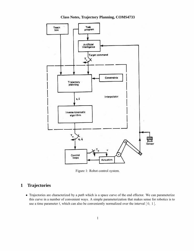
Figure 1: Robot control system.

1 Trajectories

• Trajectories are characterized by a path which is a space curve of the end effector. We can parameterizethis curve in a number of convenient ways. A simple parameterization that makes sense for robotics is touse a time parameter t, which can also be conveniently normalized over the interval [ 0, 1 ].

1

Criteria for Trajectories include:

• Efficient - easy to compute and execute

• Predictable and accurate - should not degenerate near a singularity

• Position, Velocity and Acceleration should be smooth functions of time

• The output of the trajectory planner is a sequence of arm configurations (either in joint or Cartesian space)that form the input to the feedback control system of the robot arm.

While this problem seems fairly straight forward at first glance, it is not. Complications include:

• Hand rotation also needs to be planned and controlled (e.g. last 3 joints of a 6-axis robot like a puma)

• Trajectory planning is often kinematic analysis only; the actual dynamics of the robot (acceleration of thelink masses, friction, gravity, gear backlash etc.) are usually ignored.

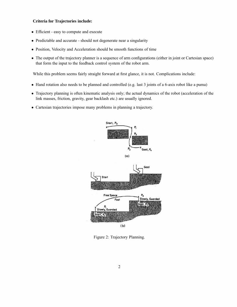
• Cartesian trajectories impose many problems in planning a trajectory.

Figure 2: Trajectory Planning.

2

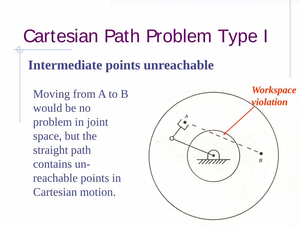
Cartesian Path Problem Type I

Workspace violation

Intermediate points unreachable

Moving from A to B would be no problem in joint space, but the straight path contains un-reachable points in Cartesian motion.

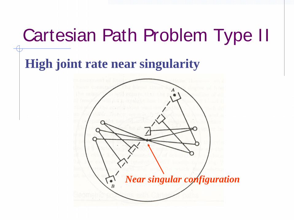
Cartesian Path Problem Type II

Near singular configuration

High joint rate near singularity

2 Joint Space Trajectories

• PRO: Actual control of the robot occurs in joint space

• PRO: Simpler to plan trajectories in real-time; less computation

• PRO: No problem with singularities

• CON: Actual robot position is sometimes unclear, particularly in presence of known obstacles (e.g. is therobot below or above the work table?)

3 Cartesian Space Trajectories

• PRO: Path we desire is usually a Cartesian path - how we reason about 3-space.

• PRO: Easy to “visualize” the trajectory

• PRO: occurs in many robotic activities- peg in hole, tracking a conveyor, welding a seam, etc.

• PRO: gives shortest Euclidean path (although not necessarily the fastest, or most energy conservative)

• PRO: straight line path minimizes inertial forces on gripper and anything it may be carrying

• PRO: Cartesian trajectory can be “robot independent”

• CON: Inverse kinematics needed, which can be multi-valued

• CON: Smooth trajectory in Cartesian space may not map to continuous joint space trajectory - wrist mayhave to flip, arm configuration may have to change

• CON: joint limits may prevent position from being realized

• CON:end-effector paths may not be safe for rest of manipulator

• CON: computational demand and analytic complexity

4 Planning a Joint Space Trajectory

• The problem in its simplest case is: given starting joint position vector q0 and ending joint position vectorq1, find intermediate joint positions over the time interval [0,1] with separate joint space trajectory foreach joint. This avoids any problems with singularities. If we can find a function f(t) that satisfies thecriteria f(0) = 0, f(1) = 1 and the range of f is the interval [0,1], then:

q(t) = f(t)q1 + (1 − f(t))q0

• If f(t) = t, then we have the case of linear interpolation between the joints.

• Problem with linear interpolation: Given a set of multiple via points, position continuity is assured, butvelocity and acceleration are not. The trajectory may be “jerky” as each point is reached, but the robotneeds to stop and then resume a new linear interpolation between the next set of points.

3

5 Polynomial Interpolation

Our choice of the function f(t) can include more constraints (i.e. velocity and acceleration) if we use a higherorder polynomial function f which still satsifies the criteria. If we choose a cubic polynomial, we can specify 4constraints that fully determine the cubic trajectory space curve.

q(t) = a t3 + b t2 + c t + d

q(t) = 3 a t2 + 2 b t + c

Parameterizing time t for the trajectory in the range [0,1] yields strating and ending positions q(0) =q0 , q(1) = q1 which are two constraints. We also can specify q(0) = v0, q(1) = v1 (starting and endingvelocities).

This yields:

q0 = d

v0 = c

q1 = a + b + c + d

v1 = 3 a + 2 b + c

Since we know the values of coefficients d and c, we can solve the last 2 equations for coefficients a and b

and fully specify the polynomial q(t).

a = 2 q0 − 2 q1 + v0 + v1

b = −v1 − 2 v0 − 3 (q0 − q1)

We can also pose this as a matrix equation, solved by inverting the leftmost matrix below:

0 0 0 10 0 1 01 1 1 13 2 1 0

a

b

c

d

=

q0

v0

q1

v1

(1)

a

b

c

d

=

2 1 −2 1−3 −2 3 −10 1 0 01 0 0 0

q0

v0

q1

v1

(2)

We can also inlcude more constraints, including intial acceleration and final acceleration and use a higherorder polynomial. Here we can specify q0 q1 v0 v1 a0 a1, the starting and ending positions, velocities, andaccelerations. These 6th constraints can be fitted with a 5th order polynomial (quintic):

q(t) = a t5 + b t4 + c t3 + d t2 + e t + f

q(t) = 5 a t4 + 4 b t3 + 3 c t2 + 2 d t + e

q(t) = 20 a t3 + 12 b t2 + 6 c t + 2 d

4

and q0 = f , q1 = a+b+c+d+e+f , v0 = e, v1 = 5a+4b+3c+2d+e, a0 = 2d, a1 = 20a+12b+6c+2d,which can be solved for the 6 co-efficients of the quintic polynomial.

0 0 0 0 0 11 1 1 1 1 10 0 0 0 1 05 4 3 2 1 00 0 0 2 0 020 12 6 2 0 0

a

b

c

d

e

f

=

q0

q1

v0

v1

a0

a1

(3)

6 Piece-wise Polynomial Interpolation

The analysis above using cubic or quintic polynomials is only good for specifying 2 endpoint positions and2 velocities (and 2 accelerations if using a quintic). However, when we get above degree 3 polynomials, weadd to our computational burden of computing the trajectory, as well as introducing trajectory curves that haveoscillations in them (a quintic has 5 roots). Even if we use a quintic, we still have to treat each set of 2 pointsseparately, which means we may have continuity at the endpoints of each trajectory segment, but not necessarilyvelocity or acceleration continuity. However, if we use the method of composite splines, we can create curvesthat are piecewise C2 continuous (continuous in position, velocity, and acceleration). The idea is to createpolynomial segments between two points in the trajectory, and include constraints that the position, velocity,and acelerations are equal where one segment ends and another begins, thus insuring smooth continuous motion.Using figure 3, we can see that:

• We have n + 1 “knot” points ( labeled 0...n)

• We need n cubic interpolating curves between each pair of points

• If each interpolating curve is a cubic, then we have 4 n constraints total that we need to find.

The constraints we can use are:

• the interior knot points are position constraints on each of 2 interpolating curves (start and end of 2different curves). There are n − 1 interior points which yield 2 (n − 1) constraints

• We can specify that the velocity at the end of one curve is the same as the velocity at the start of thenext curve to yield n − 1 constraints (this happens at each interior knot point). If we also constrain theaccelerations to be equivalent at the interior points, we generate an additional n − 1 constraints.

• The first and last knot points add 2 position constraints.

Total: 2 (n − 1) + n − 1 + n − 1 + 2 = 4n − 2 constraints.

By simply specifying 2 other constraints (starting or ending velocity or starting or ending acceleration) wecan create smooth jerk free trajectories in space. However, we are not specifying the velocites and accelerationsexplicitly at the joins of the curves, just requiring them to be smooth and continuous there.

5

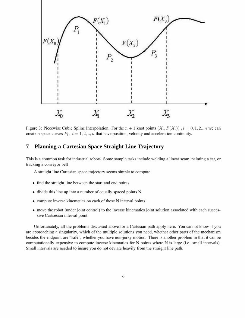
Figure 3: Piecewise Cubic Spline Interpolation. For the n + 1 knot points (Xi, F (Xi)) , i = 0, 1, 2...n we cancreate n space curves Pi , i = 1, 2, .., n that have position, velocity and acceleration continuity.

7 Planning a Cartesian Space Straight Line Trajectory

This is a common task for industrial robots. Some sample tasks include welding a linear seam, painting a car, ortracking a conveyor belt

A straight line Cartesian space trajectory seems simple to compute:

• find the straight line between the start and end points.

• divide this line up into a number of equally spaced points N.

• compute inverse kinematics on each of these N interval points.

• move the robot (under joint control) to the inverse kinematics joint solution associated with each succes-sive Cartsesian interval point

Unfortunately, all the problems discussed above for a Cartesian path apply here. You cannot know if youare approaching a singularity, which of the multiple solutions you need, whether other parts of the mechanismbesides the endpoint are “safe”, whether you have non-jerky motion. There is another problem in that it can becomputationally expensive to compute inverse kinematics for N points where N is large (i.e. small intervals).Small intervals are needed to insure you do not deviate heavily from the straight line path.

6

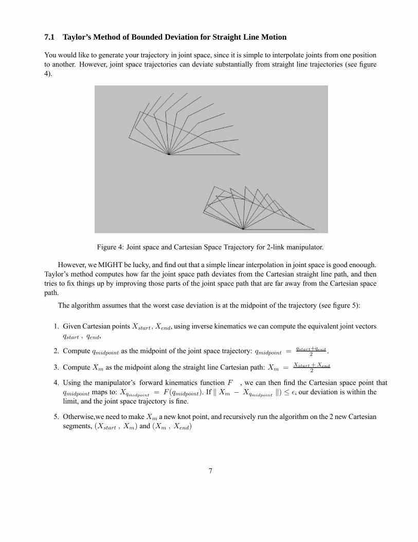
7.1 Taylor’s Method of Bounded Deviation for Straight Line Motion

You would like to generate your trajectory in joint space, since it is simple to interpolate joints from one positionto another. However, joint space trajectories can deviate substantially from straight line trajectories (see figure4).

Figure 4: Joint space and Cartesian Space Trajectory for 2-link manipulator.

However, we MIGHT be lucky, and find out that a simple linear interpolation in joint space is good enoough.Taylor’s method computes how far the joint space path deviates from the Cartesian straight line path, and thentries to fix things up by improving those parts of the joint space path that are far away from the Cartesian spacepath.

The algorithm assumes that the worst case deviation is at the midpoint of the trajectory (see figure 5):

1. Given Cartesian points Xstart, Xend, using inverse kinematics we can compute the equivalent joint vectorsqstart , qend,

2. Compute qmidpoint as the midpoint of the joint space trajectory: qmidpoint = qstart+qend

2.

3. Compute Xm as the midpoint along the straight line Cartesian path: Xm = Xstart + Xend

2

4. Using the manipulator’s forward kinematics function F , we can then find the Cartesian space point thatqmidpoint maps to: Xqmidpoint

= F (qmidpoint). If ‖ Xm − Xqmidpoint‖) ≤ ǫ, our deviation is within the

limit, and the joint space trajectory is fine.

5. Otherwise,we need to make Xm a new knot point, and recursively run the algorithm on the 2 new Cartesiansegments, (Xstart , Xm) and (Xm , Xend)

7

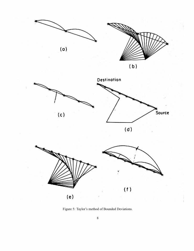
Figure 5: Taylor’s method of Bounded Deviations.

8

7.2 Resolved Rate Motion Control: Jacobian Control

We previously specified the Jacobian matrix relationship as:

[

X]

= J[

Θ]

which relarted Cartesian velocities X to joint velocities Θ. Inverting the Jacobian yields

[

J−1] [

X]

=[

Θ]

which allows us to specify Cartesian velocities and compute joint rates of change. Accordingly, we canspecify a discrete trajectory of very finely sampled points along a Cartesian path, and use Jacobian control tofind the appropriate joint rates. If we think of the finely sampled points along the Cartesian path as x1 . . . xn,then we can incrementally move an amount ∆x at each time step. This is equivalent to ∆x

∆t, or the Cartesian

velcoity between each set of adjacent, finely sampled points where

∆x = xi+1 − xi

Once we compute this set of ∆x changes, we can multiply them by the inverse Jacobian and find theresultant joint rates of change.

Although this is very straightforward, there are some caveats. First we need a closed form solution to theJacobian matrix in order to be able to invert it fast. Second, the method does not handle singularites as it assumesthe Jacobian is not singular. One needs to check on this as driving the robot through a singularity can be verypainful!

9