1-s2 0-s0142061514000064-main
TRANSCRIPT
Electrical Power and Energy Systems 58 (2014) 64–74
Contents lists available at ScienceDirect
Electrical Power and Energy Systems
journal homepage: www.elsevier .com/locate / i jepes
Small signal stability analysis of power systems with DFIG based windpower penetration
0142-0615/$ - see front matter � 2014 Elsevier Ltd. All rights reserved.http://dx.doi.org/10.1016/j.ijepes.2014.01.005
⇑ Corresponding author. Mobile: +91 9427339896.E-mail address: [email protected] (P. Bhatt).
Bhinal Mehta a, Praghnesh Bhatt a,⇑, Vivek Pandya b
a Department of Electrical Engineering, C.S. Patel Institute of Technology, CHARUSAT, Changa, Gujarat, Indiab Department of Electrical Engineering, School of Technology, PDPU, Gandhinagar, Gujarat, India
a r t i c l e i n f o a b s t r a c t
Article history:Received 12 April 2013Received in revised form 6 December 2013Accepted 2 January 2014
Keywords:Doubly fed induction generatorPower system oscillationsEigenvalue analysisWind turbine generators
With the increasing penetration of wind power generation into the power system, it is required tocomprehensively analyze its impact on power system stability. The present paper analyzes the impactof wind power penetration by doubly fed induction generator (DFIG) on power system oscillations fortwo-area interconnected power system. The aspects of inter-area oscillations which may affect the oper-ation and behaviour of the power systems are analyzed with and without the wind power penetration.Eigenvalue analysis is carried out to investigate the small signal behaviour of the test system and theparticipation factors have been determined to identify the participation of the states in the variation ofdifferent mode shapes. The penetration of DFIG in a test system results in an oscillatory instability, whichcan be stabilized with the coordinated operation of automatic voltage regulator (AVR) and power systemstabilizer (PSS) equipped on synchronous generators. Also, the variations in oscillatory modes are pre-sented to observe the damping performance of the test system at different wind power penetration level.
� 2014 Elsevier Ltd. All rights reserved.
1. Introduction
The electricity industry worldwide is turning increasingly torenewable sources of energy to generate electricity. Wind is thefastest growing and the most widely utilized emerging renewableenergy technology for power generation at present, with a total ofapproximately 250 GW installed worldwide up to 2012 [1].
The wind turbine generators (WTGs) are divided into two basiccategories: fixed speed and variable speed. A fixed-speed WTGgenerally uses a squirrel-cage induction generator (SCIG) to con-vert the mechanical energy from the wind turbine into electricalenergy. DFIG and direct drive synchronous generator (DDSG) arepopular types of variable speed WTGs. Variable-speed WTGs canoffer increased efficiency in capturing the energy from wind overa wider range of wind speeds, along with better power qualityand with the ability to regulate the power factor, by eitherconsuming or producing reactive power. In the DFIG, the rotor isconnected to the power system through the back-to-back ac/dc/ac converter, while the stator is connected directly to the powersystem. The control scheme of DFIG decouples the rotational speedof rotor from the grid frequency [2,3].
Modelling of DFIG for stability studies has lead to various mod-els developed using different approaches presented in [4–8]. Theinfluence of load increase, the length of transmission network
interface and the different penetration levels of a constant speedwind turbine generator on power system oscillations is studiedin [9] with the consideration of SCIG.
In [10], supplementary control strategy is designed for the DFIGpower converters to mitigate the impact of reduced inertia due tosignificant DFIG penetration in a large power system. Small signalbehaviour of DFIG in power factor control mode and voltage con-trol mode were extensively analyzed in [11]. Improved controllertuning is proposed to damped inter area mode oscillations. The im-pacts of DFIGs on the electromechanical modes are demonstratedto be highly dependent on their control strategies. The authors in[12,13] have reported the likelihood of the contribution of DFIGsto the system damping with application of appropriate coordinatedtuning of controllers by evolutionary techniques. In [14], an ap-proach of sensitivity analysis of electromechanical modes to theinertia of the generators is introduced and the results have shownboth detrimental and beneficial impacts of increased DFIG penetra-tion into the power system.
The dynamic behaviour of the DFIG has been investigated byvarious authors. The majority of these studies are to show theimpact of DFIG on power system dynamics, the merits of decou-pled control and maximum power tracking and the response togrid disturbances, the fault ride through behaviour, the controlmethods to make the DFIG behave like a synchronous generator[15–20]. The advanced control capabilities of DFIG are used in[21] to enhance network damping via an auxiliary power systemstabilizer loop.
B. Mehta et al. / Electrical Power and Energy Systems 58 (2014) 64–74 65
The literature survey shows that the small signal stability anal-ysis with the integration of wind power generation has been ad-dressed for single machine infinite bus system (SMIB) whereasthe less attention has been paid for multi machine system whichare equipped with AVR and PSS on synchronous machines. Themodes of response introduced by DFIG in interconnected powersystems, as well as the effect of increased penetration of DFIG oninter area oscillations considering two-area power system havebeen investigated in the present paper. The influence on modeswith the displacement of synchronous generators equipped withor without AVR and PSS are shown. Further, the effects of place-ment of DFIG at different locations and stepwise penetration ofwind power on small signal stability are analyzed in the presentwork.
The paper is organized in six sections. Section 2 presents thecharacteristics and modelling concepts associated with DFIGs.The small signal stability and eigenvalue analysis has been dis-cussed in Section 3. Section 4 details the approach developed toanalyze the impact of increased penetration of DFIGs on small sig-nal and transient stability along with case description. Simulationand results with different cases are presented and discussed in Sec-tion 5 followed by the conclusion in Section 6.
2. Characteristic and modelling of DFIG
2.1. Electrical dynamics
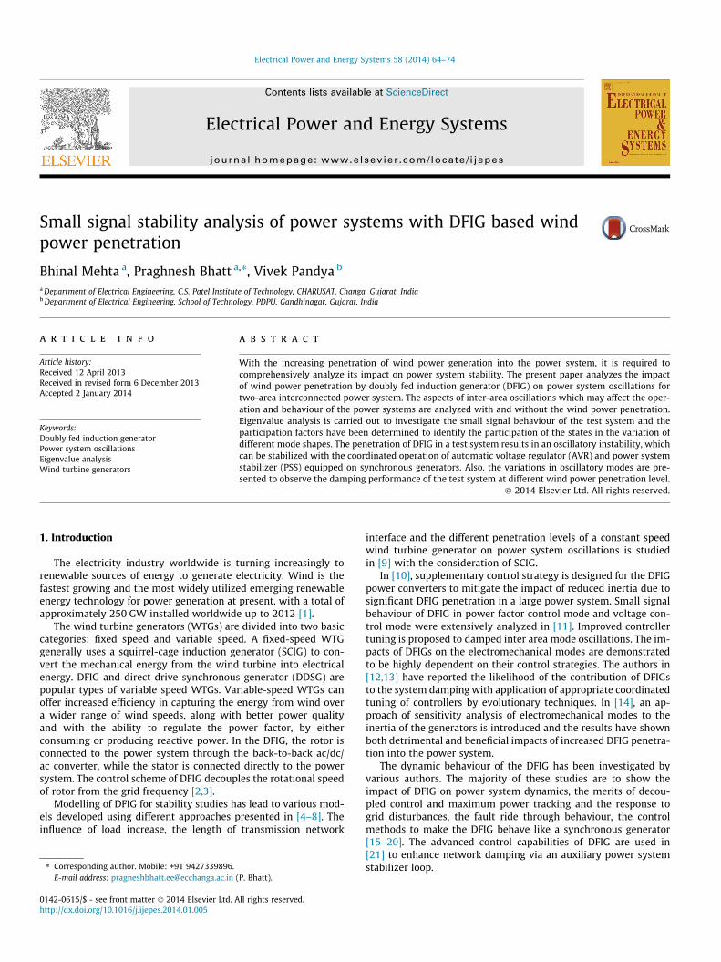
The schematic of DFIG interfaced with electrical grid is shownin Fig. 1. The stator and rotor flux dynamics of induction machineare assumed to be fast in comparison with grid dynamics and theconverter controllers decouple the generator rotational speed fromthe grid. As a result, steady-state electrical equations of DFIG canbe represented by (1)–(4) [22–25].
vds ¼ �Rsids þ ððXs þ XmÞiqs þ XmiqrÞ ð1Þ
vqs ¼ �Rsiqs � ððXs þ XmÞids þ XmidrÞ ð2Þ
vdr ¼ �Rridr þ ð1�xmÞððXr þ XmÞiqr þ XmiqsÞ ð3Þ
vqr ¼ �Rriqr � ð1�xmÞððXr þ XmÞidr þ XmidsÞ ð4Þ
where vds and vqs are d- and q-axis stator voltages, respectively, vdr
and vqr are d- and q-axis rotor voltages, respectively, ids and iqs ared- and q-axis stator currents, respectively, idr and iqr are d- andq-axis rotor currents respectively, RS is stator resistance, Rr is rotorresistance, Xs is stator reactance, Xm is magnetization reactance, Xr isrotor reactance and xm is the rotor speed.
Gear Box
Doubly Fed Induction Generator
(DFIG)
PWM Conver(Rotor SideConverter
(RSC)
SlipRings
AC low voltage andVariable frequency
Fig. 1. Schematic of DFIG integ
2.2. Power dynamics
The power injected in the grid depends on the operating modeof the converter and it is also a function of stator and rotor cur-rents. Hence, the converter powers on the grid side and rotor sideare represented by (5)–(6) and (7)–(8), respectively.
The converter powers on grid side:
Pg ¼ vdgidg þ vqgiqg ð5Þ
Qg ¼ vqgidg � vdgiqg ð6Þ
The converter powers on rotor side:
Pr ¼ vdridr þ vqriqr ð7Þ
Qr ¼ vqridr � vdriqr ð8Þ
where vdg and vqg are d- and q-axis voltages of the grid side conver-tor respectively, idg and iqg are d- and q-axis current of the grid sideconvertor, respectively.
2.3. Wind turbine dynamics
In stability studies of DFIG wind turbine, the model of drivetrain is important. It is assumed that the convertor controls areable to filter shaft dynamics and therefore the generator motionequations, which represent mechanical dynamics of wind turbine,are as follows:
_xm ¼ ðTm � TeÞ=2Hm ð9Þ
Te ¼ Xmðiqrids � idriqsÞ ð10Þ
where Te is electromagnetic torque and is approximated as follows:
Te � �XmViqr
xbðXs þ XmÞð11Þ
where xb is the system frequency rate in rad/s, Hm is inetia con-stants in kW s/kV A. The mechanical torque Tm which is the powerinput of the wind turbine is as follows:
Tm ¼Pw
xmð12Þ
where Pw the mechanical power extracted from the wind and is asfollows:
Pw ¼q2
cpðk; hpÞArv3w ð13Þ
where q is the air density, vw is the wind speed, hp is the pitch angle,Ar is the area swept by the rotor and k is the blade tip speed ratio.
ter I
)
PWM Converter II(Grid Side Converter)
(GSC)
DC
AC Side
Three Winding Transformer
LV
MVHV
ElectricalNetwork
rated with electrical grid.
66 B. Mehta et al. / Electrical Power and Energy Systems 58 (2014) 64–74
The performance co-efficient or the power co-efficient cp is asfollows:
cp ¼ 0:22116ki� 0:4hp � 5
� �e�
12:5ki ð14Þ
With1ki¼ 1
kþ 0:08hp� 0:035
h3p þ 1
ð15Þ
Cpðk; hpÞ has a maximum cmaxp for a particular tip speed ratio kopt and
pitch angle hp = 0. The aim for variable wind turbine at wind speedslower than rated value is to adjust the rotor speed at varying windspeeds; therefore, k and cp are always maintained at the optimaland maximum value, respectively. The speed control of the DFIGis achieved by driving the generator speed along the optimumpower–speed characteristic curve (see Fig. 5), which correspondsto the maximum energy capture from the wind. In this curve, whengenerator speed is less than the low limit or higher than the ratedvalue, the reference speed is set to the minimal value or rated value,respectively. When generator speed is between the lower limit andthe rated value, the rotor speed reference can be obtained by substi-tuting k into (13) as follows:
k ¼ v t
vw¼ gGB
2Rxwr
pvwð16Þ
where vt is the blade tip speed, vw the wind speed upstream the ro-tor, gGB is the gear box ratio, p is the number of poles of the induc-tion generator and R is the rotor radius.
2.4. Pitch angle control
The pitch angle of the blade is controlled to optimize the powerextraction of wind turbine as well as to prevent overrated powerproduction in strong wind. The pitch servo is modelled as follows:
_hp ¼ ðKp£ðxm �xref Þ � hpÞ=Tp ð17Þ
where £ is a function which allows varying the pitch angle setpoint only when the difference (xm �xref) exceeds a predefined va-lue ±Dx.
For the sake of simplicity, the reference of the pitch angle hp = 0when wind speed is below rated value. When wind speed is higherthan rated value, the power limitation is active by adjusting thepitch angle using the pitch-control scheme shown in Fig. 2.
2.5. Converter dynamics
The ac–dc–ac converter model in DFIG system comprises of twopulse width modulation invertors connected back to back via dclink as shown in Fig. 1. The rotor side converter (RSC) and the gridside converter (GSC) act as a controlled voltage source and con-trolled current source, respectively. The RSC injects an ac voltageat slip frequency to the DFIG rotor, whereas the GSC injects an accurrent at grid frequency to the network and maintains the dc-linkvoltage constant.
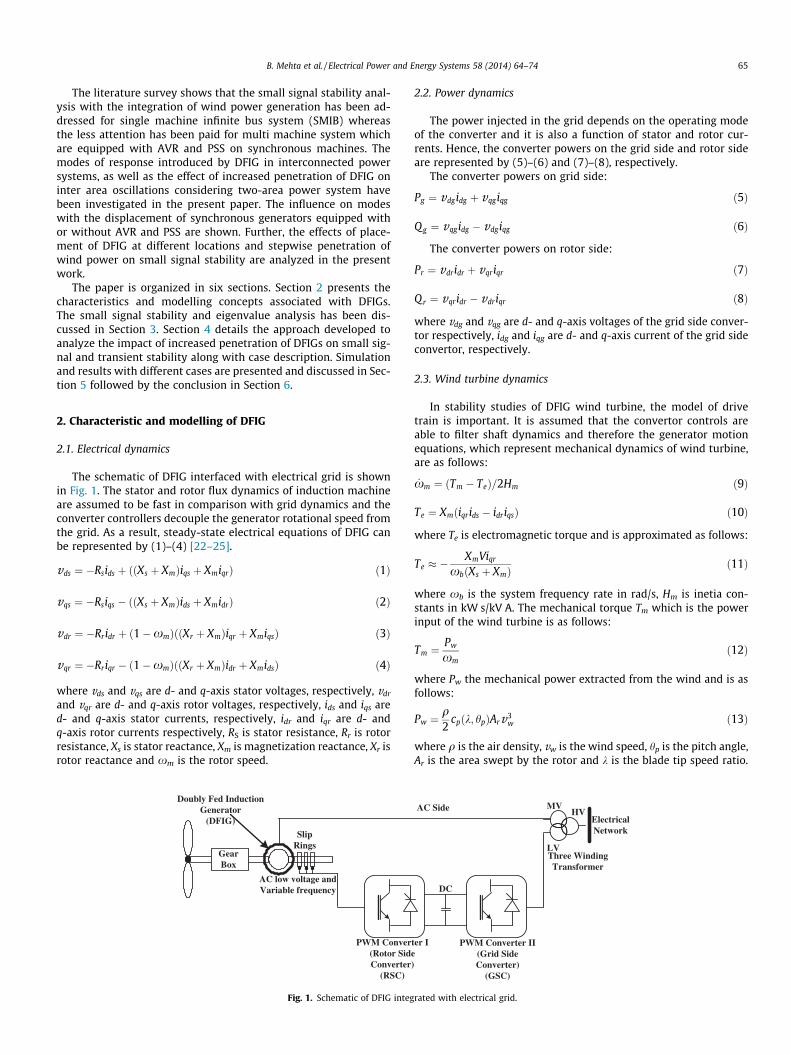
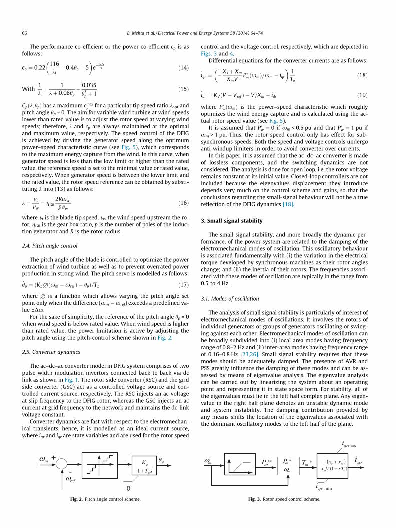
Converter dynamics are fast with respect to the electromechan-ical transients, hence, it is modelled as an ideal current source,where iqr and iqr are state variables and are used for the rotor speed
Fig. 2. Pitch angle control scheme.
control and the voltage control, respectively, which are depicted inFigs. 3 and 4.
Differential equations for the converter currents are as follows:
_iqr ¼ �Xs þ Xm
XmVP�wðxmÞ=xm � iqr
� �1Te
ð18Þ
_idr ¼ KV ðV � Vref Þ � V=Xm � idr ð19Þ
where P�wðxmÞ is the power–speed characteristic which roughlyoptimizes the wind energy capture and is calculated using the ac-tual rotor speed value (see Fig. 5).
It is assumed that P�w ¼ 0 if xm < 0.5 pu and that P�w ¼ 1 pu ifxm > 1 pu. Thus, the rotor speed control only has effect for sub-synchronous speeds. Both the speed and voltage controls undergoanti-windup limiters in order to avoid converter over currents.
In this paper, it is assumed that the ac–dc–ac converter is madeof lossless components, and the switching dynamics are notconsidered. The analysis is done for open loop, i.e. the rotor voltageremains constant at its initial value. Closed-loop controllers are notincluded because the eigenvalues displacement they introducedepends very much on the control scheme and gains, so that theconclusions regarding the small-signal behaviour will not be a truereflection of the DFIG dynamics [18].
3. Small signal stability
The small signal stability, and more broadly the dynamic per-formance, of the power system are related to the damping of theelectromechanical modes of oscillation. This oscillatory behaviouris associated fundamentally with (i) the variation in the electricaltorque developed by synchronous machines as their rotor angleschange; and (ii) the inertia of their rotors. The frequencies associ-ated with these modes of oscillation are typically in the range from0.5 to 4 Hz.
3.1. Modes of oscillation
The analysis of small signal stability is particularly of interest ofelectromechanical modes of oscillations. It involves the rotors ofindividual generators or groups of generators oscillating or swing-ing against each other. Electromechanical modes of oscillation canbe broadly subdivided into (i) local area modes having frequencyrange of 0.8–2 Hz and (ii) inter-area modes having frequency rangeof 0.16–0.8 Hz [23,26]. Small signal stability requires that thesemodes should be adequately damped. The presence of AVR andPSS greatly influence the damping of these modes and can be as-sessed by means of eigenvalue analysis. The eigenvalue analysiscan be carried out by linearizing the system about an operatingpoint and representing it in state space form. For stability, all ofthe eigenvalues must lie in the left half complex plane. Any eigen-value in the right half plane denotes an unstable dynamic modeand system instability. The damping contribution provided byany means shifts the location of the eigenvalues associated withthe dominant oscillatory modes to the left half of the plane.
Fig. 3. Rotor speed control scheme.
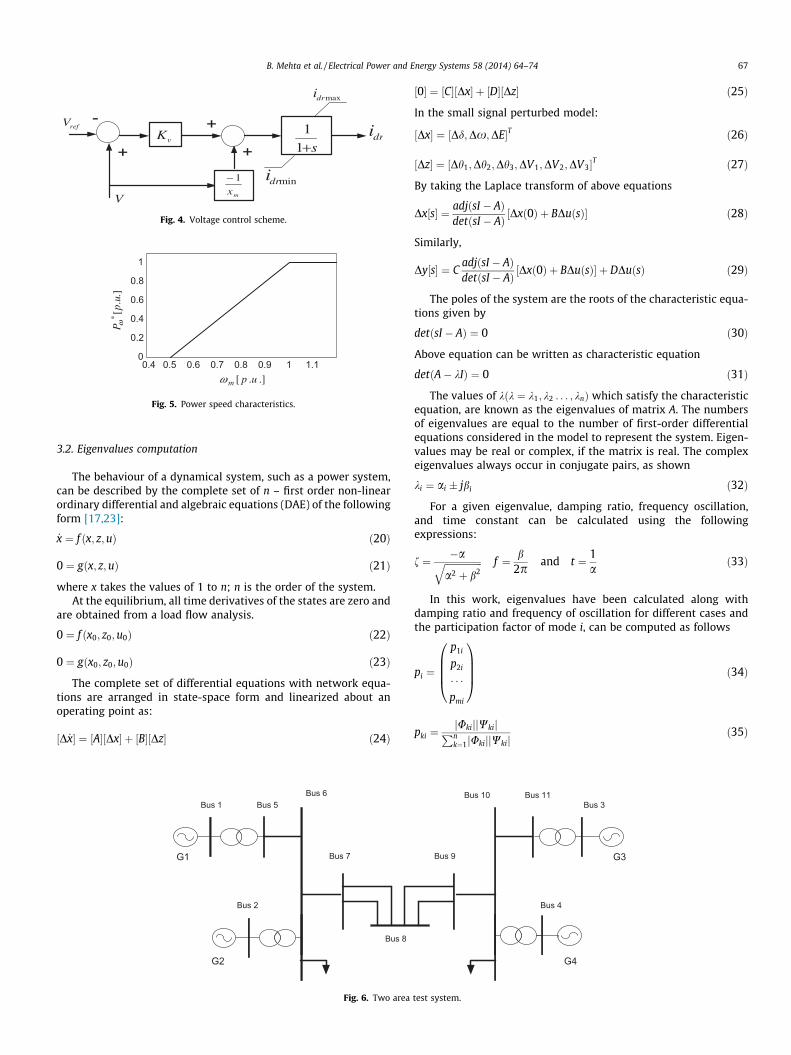
Fig. 4. Voltage control scheme.
.].
[*
up
P ω
.].[ upmω0.4
0.8
0.4
0.6
1
0.2
00.60.5 0.7 0.8 0.9 1 1.1
Fig. 5. Power speed characteristics.
B. Mehta et al. / Electrical Power and Energy Systems 58 (2014) 64–74 67
3.2. Eigenvalues computation
The behaviour of a dynamical system, such as a power system,can be described by the complete set of n – first order non-linearordinary differential and algebraic equations (DAE) of the followingform [17,23]:
_x ¼ f ðx; z;uÞ ð20Þ
0 ¼ gðx; z;uÞ ð21Þ
where x takes the values of 1 to n; n is the order of the system.At the equilibrium, all time derivatives of the states are zero and
are obtained from a load flow analysis.
0 ¼ f ðx0; z0;u0Þ ð22Þ
0 ¼ gðx0; z0;u0Þ ð23Þ
The complete set of differential equations with network equa-tions are arranged in state-space form and linearized about anoperating point as:
½D _x� ¼ ½A�½Dx� þ ½B�½Dz� ð24Þ
G1
G2
Bus 1
Bus 2
Bus 5Bus 6
Bus 8
Bus 7
Fig. 6. Two area
½0� ¼ ½C�½Dx� þ ½D�½Dz� ð25Þ
In the small signal perturbed model:
½Dx� ¼ ½Dd;Dx;DE�T ð26Þ
½Dz� ¼ ½Dh1;Dh2;Dh3;DV1;DV2;DV3�T ð27Þ
By taking the Laplace transform of above equations
Dx½s� ¼ adjðsI � AÞdetðsI � AÞ ½Dxð0Þ þ BDuðsÞ� ð28Þ
Similarly,
Dy½s� ¼ CadjðsI � AÞdetðsI � AÞ ½Dxð0Þ þ BDuðsÞ� þ DDuðsÞ ð29Þ
The poles of the system are the roots of the characteristic equa-tions given by
detðsI � AÞ ¼ 0 ð30Þ
Above equation can be written as characteristic equation
detðA� kIÞ ¼ 0 ð31Þ
The values of kðk ¼ k1; k2 . . . ; knÞ which satisfy the characteristicequation, are known as the eigenvalues of matrix A. The numbersof eigenvalues are equal to the number of first-order differentialequations considered in the model to represent the system. Eigen-values may be real or complex, if the matrix is real. The complexeigenvalues always occur in conjugate pairs, as shown
ki ¼ ai � jbi ð32Þ
For a given eigenvalue, damping ratio, frequency oscillation,and time constant can be calculated using the followingexpressions:
f ¼ �affiffiffiffiffiffiffiffiffiffiffiffiffiffiffiffia2 þ b2
q f ¼ b2p
and t ¼ 1a
ð33Þ
In this work, eigenvalues have been calculated along withdamping ratio and frequency of oscillation for different cases andthe participation factor of mode i, can be computed as follows
pi ¼
p1i
p2i
� � �pmi
0BBB@
1CCCA ð34Þ
pki ¼jUkijjWkijPnk¼1jUkijjWkij
ð35Þ
G3
G4
Bus 10 Bus 11Bus 3
Bus 4
Bus 9
test system.
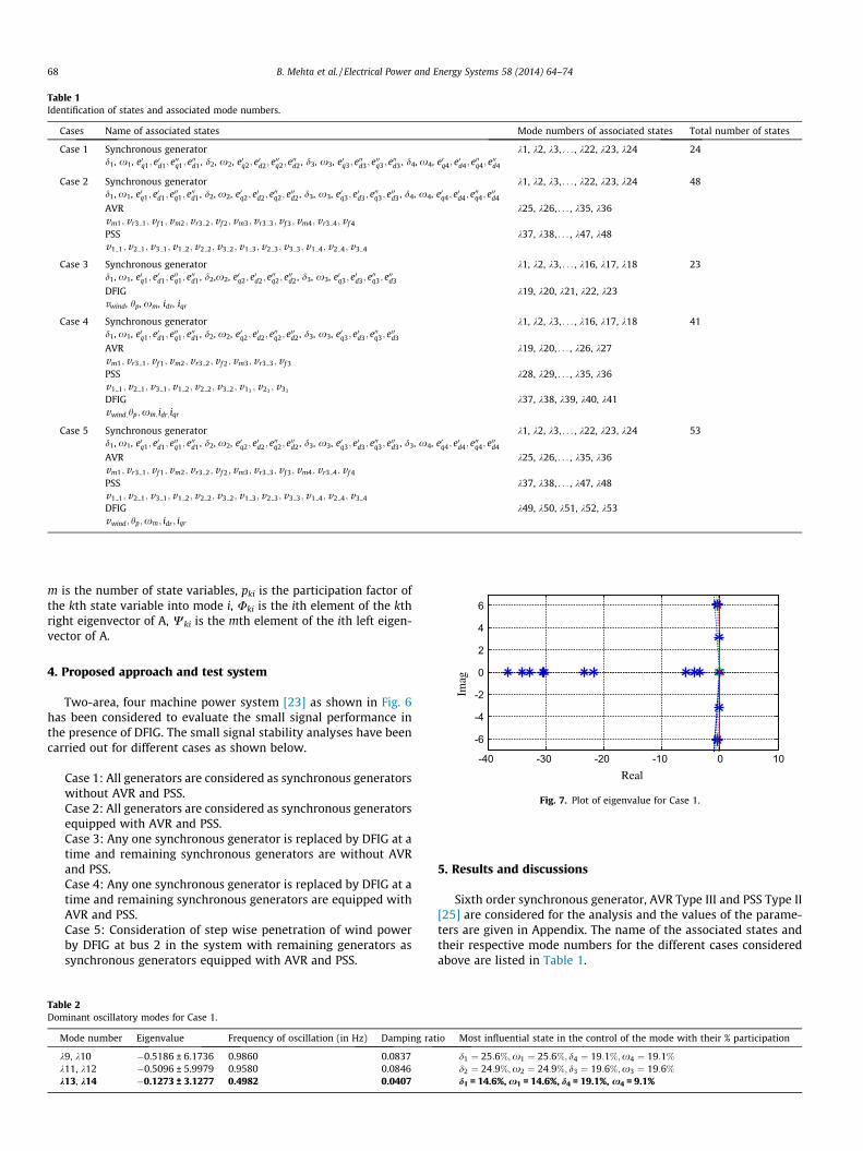
Table 1Identification of states and associated mode numbers.
Cases Name of associated states Mode numbers of associated states Total number of states
Case 1 Synchronous generator k1, k2, k3, . . . , k22, k23, k24 24d1, x1, e0q1; e
0d1; e
00q1; e
00d1, d2, x2, e0q2; e
0d2; e
00q2; e
00d2, d3, x3, e0q3; e
00d3; e
00q3; e
00d3, d4, x4, e0q4; e
0d4; e
00q4; e
00d4
Case 2 Synchronous generator k1, k2, k3, . . . , k22, k23, k24 48d1, x1, e0q1; e
0d1; e
00q1; e
00d1, d2, x2, e0q2; e
0d2; e
00q2; e
00d2, d3, x3, e0q3; e
0d3; e
00q3; e
00d3, d4, x4, e0q4; e
0d4; e
00q4; e
00d4
AVR k25, k26, . . . , k35, k36vm1;vr3 1; v f 1;vm2; vr3 2;v f 2; vm3;vr3 3; v f 3;vm4; vr3 4;v f 4
PSS k37, k38, . . . , k47, k48v1 1;v2 1;v3 1;v1 2; v2 2; v3 2; v1 3;v2 3;v3 3;v1 4; v2 4; v3 4
Case 3 Synchronous generator k1, k2, k3, . . . , k16, k17, k18 23d1, x1, e0q1; e
0d1; e
00q1; e
00d1, d2,x2, e0q2; e
0d2; e
00q2; e
00d2, d3, x3, e0q3; e
0d3; e
00q3; e
00d3
DFIG k19, k20, k21, k22, k23vwind, hp, xm, idr, iqr
Case 4 Synchronous generator k1, k2, k3, . . . , k16, k17, k18 41d1, x1, e0q1; e
0d1; e
00q1; e
00d1, d2, x2, e0q2; e
0d2; e
00q2; e
00d2, d3, x3, e0q3; e
0d3; e
00q3; e
00d3
AVR k19, k20, . . . , k26, k27vm1;vr3 1; v f 1;vm2; vr3 2;v f 2; vm3;vr3 3; v f 3
PSS k28, k29, . . . , k35, k36v1 1;v2 1;v3 1;v1 2; v2 2; v3 2; v13 ; v23 ; v33
DFIG k37, k38, k39, k40, k41vwind;hp;xm;idr;iqr
Case 5 Synchronous generator k1, k2, k3, . . . , k22, k23, k24 53d1, x1, e0q1; e
0d1; e
00q1; e
00d1, d2, x2, e0q2; e
0d2; e
00q2; e
00d2, d3, x3, e0q3; e
0d3; e
00q3; e
00d3, d3, x4, e0q4; e
0d4; e
00q4; e
00d4
AVR k25, k26, . . . , k35, k36vm1;vr3 1; v f 1;vm2; vr3 2;v f 2; vm3;vr3 3; v f 3;vm4; vr3 4;v f 4
PSS k37, k38, . . . , k47, k48v1 1;v2 1;v3 1;v1 2; v2 2; v3 2; v1 3;v2 3;v3 3;v1 4; v2 4; v3 4
DFIG k49, k50, k51, k52, k53vwind; hp ;xm; idr ; iqr
4
6
68 B. Mehta et al. / Electrical Power and Energy Systems 58 (2014) 64–74
m is the number of state variables, pki is the participation factor ofthe kth state variable into mode i, Uki is the ith element of the kthright eigenvector of A, Wki is the mth element of the ith left eigen-vector of A.
-40 -30 -20 -10 0 10
-6
-4
-2
0
2
Real
Imag
Fig. 7. Plot of eigenvalue for Case 1.
4. Proposed approach and test system
Two-area, four machine power system [23] as shown in Fig. 6has been considered to evaluate the small signal performance inthe presence of DFIG. The small signal stability analyses have beencarried out for different cases as shown below.
Case 1: All generators are considered as synchronous generatorswithout AVR and PSS.Case 2: All generators are considered as synchronous generatorsequipped with AVR and PSS.Case 3: Any one synchronous generator is replaced by DFIG at atime and remaining synchronous generators are without AVRand PSS.Case 4: Any one synchronous generator is replaced by DFIG at atime and remaining synchronous generators are equipped withAVR and PSS.Case 5: Consideration of step wise penetration of wind powerby DFIG at bus 2 in the system with remaining generators assynchronous generators equipped with AVR and PSS.
Table 2Dominant oscillatory modes for Case 1.
Mode number Eigenvalue Frequency of oscillation (in Hz) Damping rat
k9, k10 �0.5186 ± 6.1736 0.9860 0.0837k11, k12 �0.5096 ± 5.9979 0.9580 0.0846k13, k14 �0.1273 ± 3.1277 0.4982 0.0407
5. Results and discussions
Sixth order synchronous generator, AVR Type III and PSS Type II[25] are considered for the analysis and the values of the parame-ters are given in Appendix. The name of the associated states andtheir respective mode numbers for the different cases consideredabove are listed in Table 1.
io Most influential state in the control of the mode with their % participation
d1 ¼ 25:6%;x1 ¼ 25:6%; d4 ¼ 19:1%;x4 ¼ 19:1%
d2 ¼ 24:9%;x2 ¼ 24:9%; d3 ¼ 19:6%;x3 ¼ 19:6%
d1 = 14.6%, x1 = 14.6%, d4 = 19.1%, x4 = 9.1%
-40 -30 -20 -10 0 10
-20
-10
0
10
20
Real
Imag
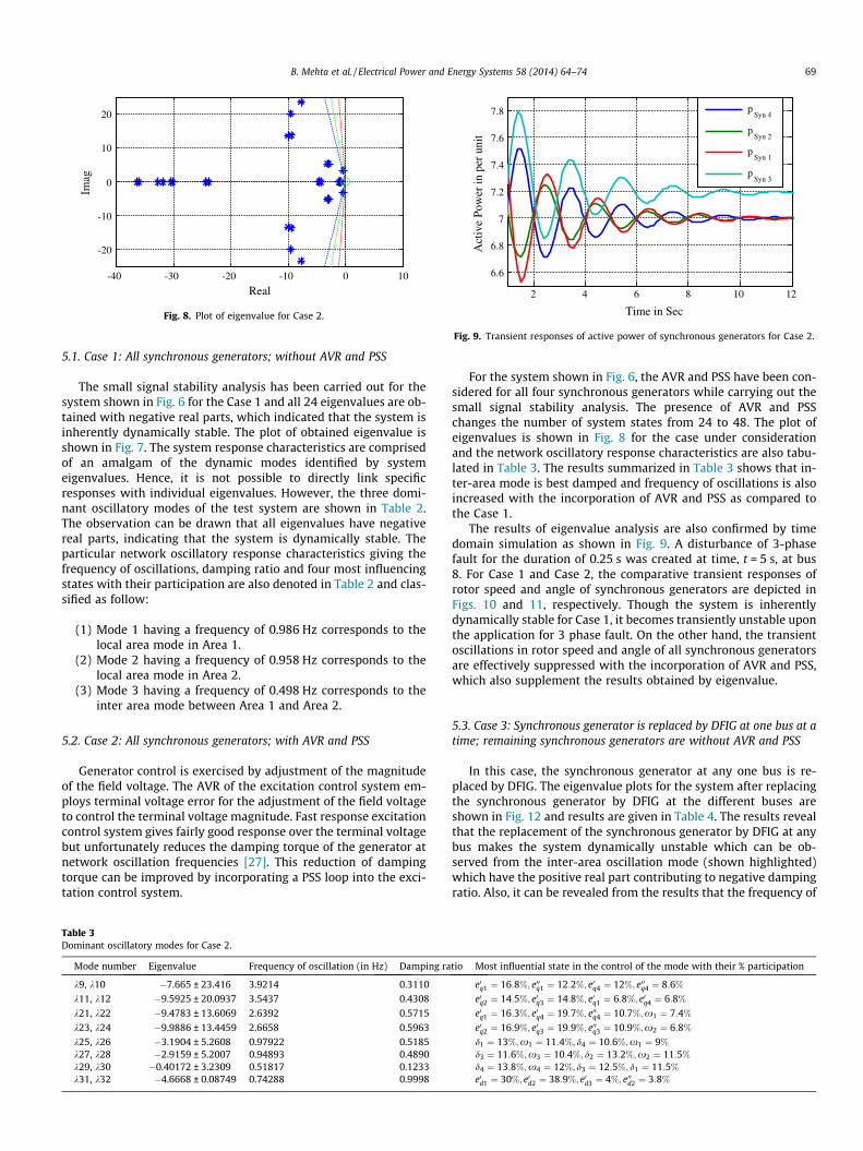
Fig. 8. Plot of eigenvalue for Case 2.
2 4 6 8 10 12
6.6
6.8
7
7.2
7.4
7.6
7.8
Time in Sec
Act
ive
Pow
er in
per
uni
t
pSyn 4
pSyn 2
pSyn 1
pSyn 3
Fig. 9. Transient responses of active power of synchronous generators for Case 2.
B. Mehta et al. / Electrical Power and Energy Systems 58 (2014) 64–74 69
5.1. Case 1: All synchronous generators; without AVR and PSS
The small signal stability analysis has been carried out for thesystem shown in Fig. 6 for the Case 1 and all 24 eigenvalues are ob-tained with negative real parts, which indicated that the system isinherently dynamically stable. The plot of obtained eigenvalue isshown in Fig. 7. The system response characteristics are comprisedof an amalgam of the dynamic modes identified by systemeigenvalues. Hence, it is not possible to directly link specificresponses with individual eigenvalues. However, the three domi-nant oscillatory modes of the test system are shown in Table 2.The observation can be drawn that all eigenvalues have negativereal parts, indicating that the system is dynamically stable. Theparticular network oscillatory response characteristics giving thefrequency of oscillations, damping ratio and four most influencingstates with their participation are also denoted in Table 2 and clas-sified as follow:
(1) Mode 1 having a frequency of 0.986 Hz corresponds to thelocal area mode in Area 1.
(2) Mode 2 having a frequency of 0.958 Hz corresponds to thelocal area mode in Area 2.
(3) Mode 3 having a frequency of 0.498 Hz corresponds to theinter area mode between Area 1 and Area 2.
5.2. Case 2: All synchronous generators; with AVR and PSS
Generator control is exercised by adjustment of the magnitudeof the field voltage. The AVR of the excitation control system em-ploys terminal voltage error for the adjustment of the field voltageto control the terminal voltage magnitude. Fast response excitationcontrol system gives fairly good response over the terminal voltagebut unfortunately reduces the damping torque of the generator atnetwork oscillation frequencies [27]. This reduction of dampingtorque can be improved by incorporating a PSS loop into the exci-tation control system.
Table 3Dominant oscillatory modes for Case 2.
Mode number Eigenvalue Frequency of oscillation (in Hz) Damping ra
k9, k10 �7.665 ± 23.416 3.9214 0.3110
k11, k12 �9.5925 ± 20.0937 3.5437 0.4308
k21, k22 �9.4783 ± 13.6069 2.6392 0.5715
k23, k24 �9.9886 ± 13.4459 2.6658 0.5963
k25, k26 �3.1904 ± 5.2608 0.97922 0.5185k27, k28 �2.9159 ± 5.2007 0.94893 0.4890k29, k30 �0.40172 ± 3.2309 0.51817 0.1233k31, k32 �4.6668 ± 0.08749 0.74288 0.9998
For the system shown in Fig. 6, the AVR and PSS have been con-sidered for all four synchronous generators while carrying out thesmall signal stability analysis. The presence of AVR and PSSchanges the number of system states from 24 to 48. The plot ofeigenvalues is shown in Fig. 8 for the case under considerationand the network oscillatory response characteristics are also tabu-lated in Table 3. The results summarized in Table 3 shows that in-ter-area mode is best damped and frequency of oscillations is alsoincreased with the incorporation of AVR and PSS as compared tothe Case 1.
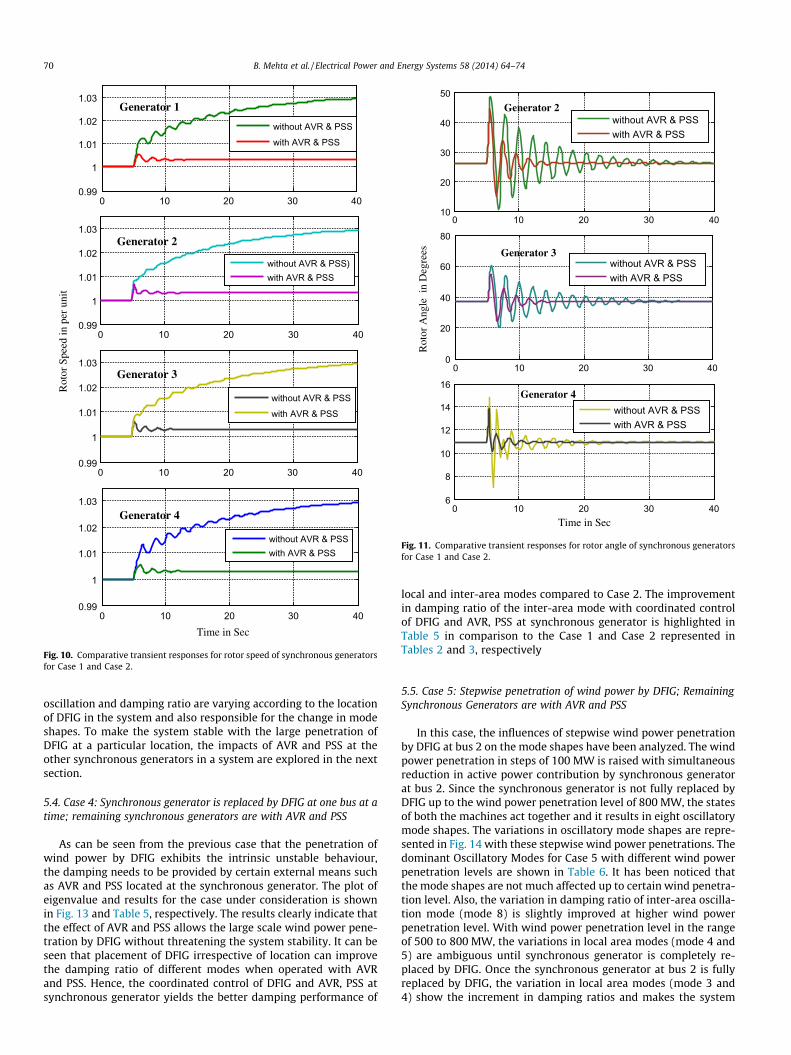
The results of eigenvalue analysis are also confirmed by timedomain simulation as shown in Fig. 9. A disturbance of 3-phasefault for the duration of 0.25 s was created at time, t = 5 s, at bus8. For Case 1 and Case 2, the comparative transient responses ofrotor speed and angle of synchronous generators are depicted inFigs. 10 and 11, respectively. Though the system is inherentlydynamically stable for Case 1, it becomes transiently unstable uponthe application for 3 phase fault. On the other hand, the transientoscillations in rotor speed and angle of all synchronous generatorsare effectively suppressed with the incorporation of AVR and PSS,which also supplement the results obtained by eigenvalue.
5.3. Case 3: Synchronous generator is replaced by DFIG at one bus at atime; remaining synchronous generators are without AVR and PSS
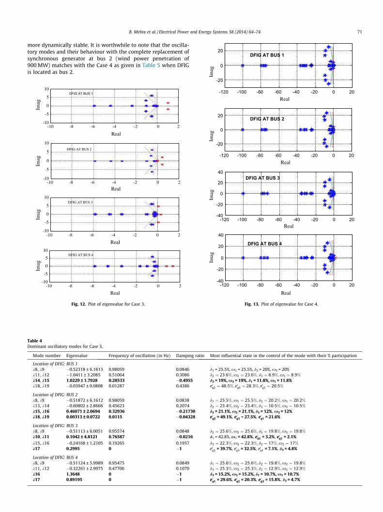
In this case, the synchronous generator at any one bus is re-placed by DFIG. The eigenvalue plots for the system after replacingthe synchronous generator by DFIG at the different buses areshown in Fig. 12 and results are given in Table 4. The results revealthat the replacement of the synchronous generator by DFIG at anybus makes the system dynamically unstable which can be ob-served from the inter-area oscillation mode (shown highlighted)which have the positive real part contributing to negative dampingratio. Also, it can be revealed from the results that the frequency of
tio Most influential state in the control of the mode with their % participation
e0q1 ¼ 16:8%; e00q1 ¼ 12:2%; e0q4 ¼ 12%; e00q4 ¼ 8:6%
e0q2 ¼ 14:5%; e0q3 ¼ 14:8%; e0q1 ¼ 6:8%; e0q4 ¼ 6:8%
e0q1 ¼ 16:3%; e0q4 ¼ 19:7%; e00q4 ¼ 10:7%;x1 ¼ 7:4%
e0q2 ¼ 16:9%; e0q3 ¼ 19:9%; e00q3 ¼ 10:9%;x2 ¼ 6:8%
d1 ¼ 13%;x1 ¼ 11:4%; d4 ¼ 10:6%;x1 ¼ 9%
d3 ¼ 11:6%;x3 ¼ 10:4%; d2 ¼ 13:2%;x2 ¼ 11:5%
d4 ¼ 13:8%;x4 ¼ 12%; d3 ¼ 12:5%; d1 ¼ 11:5%
e0d1 ¼ 30%; e0d2 ¼ 38:9%; e0d3 ¼ 4%; e00d2 ¼ 3:8%
0 10 20 30 400.99
1
1.01
1.02
1.03
Time in Seconds
Generator 1
0 10 20 30 400.99
1
1.01
1.02
1.03
Time in Seconds
Generator 2
0 10 20 30 400.99
1
1.01
1.02
1.03Generator 3
0 10 20 30 400.99
1
1.01
1.02
1.03
Time in Sec
Rot
or S
peed
in p
er u
nit
Generator 4
without AVR & PSS
with AVR & PSS
without AVR & PSS)with AVR & PSS
without AVR & PSS
with AVR & PSS
without AVR & PSSwith AVR & PSS
Fig. 10. Comparative transient responses for rotor speed of synchronous generatorsfor Case 1 and Case 2.
0 10 20 30 4010
20
30
40
50Generator 2
0 10 20 30 400
20
40
60
80
Generator 3
Rot
or A
ngle
in
Deg
rees
without AVR & PSSwith AVR & PSS
0 10 20 30 406
8
10
12
14
16
Time in Sec
Generator 4
without AVR & PSSwith AVR & PSS
without AVR & PSSwith AVR & PSS
Fig. 11. Comparative transient responses for rotor angle of synchronous generatorsfor Case 1 and Case 2.
70 B. Mehta et al. / Electrical Power and Energy Systems 58 (2014) 64–74
oscillation and damping ratio are varying according to the locationof DFIG in the system and also responsible for the change in modeshapes. To make the system stable with the large penetration ofDFIG at a particular location, the impacts of AVR and PSS at theother synchronous generators in a system are explored in the nextsection.
5.4. Case 4: Synchronous generator is replaced by DFIG at one bus at atime; remaining synchronous generators are with AVR and PSS
As can be seen from the previous case that the penetration ofwind power by DFIG exhibits the intrinsic unstable behaviour,the damping needs to be provided by certain external means suchas AVR and PSS located at the synchronous generator. The plot ofeigenvalue and results for the case under consideration is shownin Fig. 13 and Table 5, respectively. The results clearly indicate thatthe effect of AVR and PSS allows the large scale wind power pene-tration by DFIG without threatening the system stability. It can beseen that placement of DFIG irrespective of location can improvethe damping ratio of different modes when operated with AVRand PSS. Hence, the coordinated control of DFIG and AVR, PSS atsynchronous generator yields the better damping performance of
local and inter-area modes compared to Case 2. The improvementin damping ratio of the inter-area mode with coordinated controlof DFIG and AVR, PSS at synchronous generator is highlighted inTable 5 in comparison to the Case 1 and Case 2 represented inTables 2 and 3, respectively
5.5. Case 5: Stepwise penetration of wind power by DFIG; RemainingSynchronous Generators are with AVR and PSS
In this case, the influences of stepwise wind power penetrationby DFIG at bus 2 on the mode shapes have been analyzed. The windpower penetration in steps of 100 MW is raised with simultaneousreduction in active power contribution by synchronous generatorat bus 2. Since the synchronous generator is not fully replaced byDFIG up to the wind power penetration level of 800 MW, the statesof both the machines act together and it results in eight oscillatorymode shapes. The variations in oscillatory mode shapes are repre-sented in Fig. 14 with these stepwise wind power penetrations. Thedominant Oscillatory Modes for Case 5 with different wind powerpenetration levels are shown in Table 6. It has been noticed thatthe mode shapes are not much affected up to certain wind penetra-tion level. Also, the variation in damping ratio of inter-area oscilla-tion mode (mode 8) is slightly improved at higher wind powerpenetration level. With wind power penetration level in the rangeof 500 to 800 MW, the variations in local area modes (mode 4 and5) are ambiguous until synchronous generator is completely re-placed by DFIG. Once the synchronous generator at bus 2 is fullyreplaced by DFIG, the variation in local area modes (mode 3 and4) show the increment in damping ratios and makes the system
0
20
mag
DFIG AT BUS 1
B. Mehta et al. / Electrical Power and Energy Systems 58 (2014) 64–74 71
more dynamically stable. It is worthwhile to note that the oscilla-tory modes and their behaviour with the complete replacement ofsynchronous generator at bus 2 (wind power penetration of900 MW) matches with the Case 4 as given in Table 5 when DFIGis located as bus 2.
-10 -8 -6 -4 -2 0 2-10
-5
0
5
10
Real
Real
Real
Real
Imag
Imag
Imag
Imag
DFIG AT BUS 1
-10 -8 -6 -4 -2 0 2-10
-5
0
5
10DFIG AT BUS 2
-10 -8 -6 -4 -2 0 2-10
-5
0
5
10DFIG AT BUS 3
-10 -8 -6 -4 -2 0 2-10
-5
0
5
10DFIG AT BUS 4
Fig. 12. Plot of eigenvalue for Case 3.
Table 4Dominant oscillatory modes for Case 3.
Mode number Eigenvalue Frequency of oscillation (in Hz) Damping ratio Most influential state in the control of the mode with their % participation
Location of DFIG: BUS 1k8, k9 �0.52318 ± 6.1613 0.98059 0.0846 d1 = 25.5%, x1 = 25.5%, d3 = 20%, x3 = 20%k11, k12 �1.0411 ± 3.2085 0.51064 0.3086 d2 ¼ 23:6%;x2 ¼ 23:6%; d3 ¼ 8:9%;x3 ¼ 8:9%
k14, k15 1.0229 ± 1.7928 0.28533 �0.4955 d2 = 19%, x2 = 19%, d1 = 11.8%, x1 = 11.8%k18, k19 �0.03947 ± 0.0808 0.01287 0.4386 e0q2 ¼ 48:5%; e0q3 ¼ 28:3%; e0q1 ¼ 20:5%
Location of DFIG: BUS 2k8, k9 �0.51872 ± 6.1612 0.98059 0.0838 d1 ¼ 25:5%;x1 ¼ 25:5%; d3 ¼ 20:2%;x3 ¼ 20:2%
k13, k14 �0.60802 ± 2.8666 0.45623 0.2074 d2 ¼ 23:4%;x2 ¼ 23:4%; d3 ¼ 10:5%;x3 ¼ 10:5%
k15, k16 0.46071 ± 2.0694 0.32936 �0.21730 d2 = 21.1%, x2 = 21.1%, d3 = 12%, x3 = 12%k18, k19 0.00313 ± 0.0722 0.0115 �0.04328 e0q2 = 49.1%, e0q3 = 27.5%, e0q1 = 21.6%
Location of DFIG: BUS 3k8, k9 �0.51113 ± 6.0051 0.95574 0.0848 d2 ¼ 25:6%;x2 ¼ 25:6%; d3 ¼ 19:8%;x3 ¼ 19:8%
k10, k11 0.1042 ± 4.8121 0.76587 �0.0216 d1 = 42.8%, x1 = 42.8%, e0d1 = 3.2%, e0q1 = 2.1%
k15, k16 �0.24168 ± 1.2105 0.19265 0.1957 d3 ¼ 22:3%;x3 ¼ 22:3%; d2 ¼ 17%;x2 ¼ 17%
k17 0.2995 0 �1 e0q2 = 39.7%, e0q3 = 32.5%, e0q1 = 7.1%, d3 = 4.8%
Location of DFIG: BUS 4k8, k9 �0.51124 ± 5.9989 0.95475 0.0849 d1 ¼ 25:6%;x2 ¼ 25:6%; d2 ¼ 19:8%;x2 ¼ 19:8%
k11, k12 �0.32261 ± 2.9975 0.47706 0.1070 d3 ¼ 25:3%;x3 ¼ 25:3%; d2 ¼ 12:9%;x2 ¼ 12:9%
k16 1.3648 0 �1 d3 = 15.2%, x3 = 15.2%, d1 = 10.7%, x1 = 10.7%k17 0.89195 0 �1 e0q1 = 29.6%, e0q2 = 20.3%, e0q3 = 15.8%, d3 = 4.7%
-120 -100 -80 -60 -40 -20 0 20
-20
Real
I
-120 -100 -80 -60 -40 -20 0 20
-20
0
20
Real
Imag
DFIG AT BUS 2
-120 -100 -80 -60 -40 -20 0 20-40
-20
0
20
40
Real
Imag
DFIG AT BUS 3
-120 -100 -80 -60 -40 -20 0 20-40
-20
0
20
40
Real
Imag
DFIG AT BUS 4
Fig. 13. Plot of eigenvalue for Case 4.
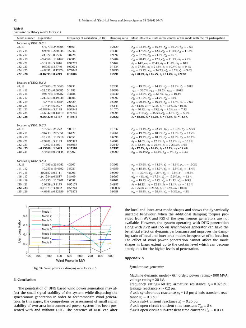
Table 5Dominant oscillatory modes for Case 4.
Mode number Eigenvalue Frequency of oscillation (in Hz) Damping ratio Most influential state in the control of the mode with their % participation
Location of DFIG: BUS 1k8, k9 �5.4273 ± 24.9008 4.0561 0.2129 e0q2 ¼ 23:1%; e00q2 ¼ 15:4%; e0q1 ¼ 10:7%; e00q1 ¼ 7:5%
k14, k15 �8.9891 ± 20.0948 3.5036 0.4083 e0q2 ¼ 17:9%; e0q1 ¼ 12%; e00q2 ¼ 11:8%; e0q3 ¼ 11:8%
k16, k17 �24.327 ± 0.5506 3.8728 0.9997 e00q2 ¼ 37:2%; e00d3 ¼ 23:8%; e00d1 ¼ 16:5,
k18, k19 �9.4566 ± 13.6167 2.6385 0.5704 e0q3 ¼ 20:4%; e0q1 ¼ 17%; e00q3 ¼ 11:1%;x1 ¼ 7:7%
k20, k21 �3.1718 ± 5.2616 0.97779 0.5162 d1 ¼ 14%;x1 ¼ 12:4%; d3 ¼ 11:8%;x3 ¼ 10%
k22, k23 �0.5083 ± 3.7749 0.60621 0.1334 d2 ¼ 27:8%;x2 ¼ 21:8%; d3 ¼ 10:4%;x3 ¼ 9:1%
k24, k25 �4.8391 ± 0.12474 0.77042 0.9996 e0d2 ¼ 35:7%; ;e0d2 ¼ 34:2%; e00d2 ¼ 3:7%; e0d2 ¼ 3:6%
k27, k28 �0.16995 ± 0.7219 0.11805 0.2291 d2 = 20.3%, d1 = 16.7%, d3 = 11.4%, x2 = 9.7%
Location of DFIG: BUS 2k8, k9 �7.2263 ± 23.5663 3.9231 0.2931 e0q1 ¼ 19:9%; e00q1 ¼ 14:2%; e0q3 ¼ 13:8%; e00q3 ¼ 9:8%
k11, k12 �32.535 ± 0.06085 5.1782 0.9999 v2 1 ¼ 36:7%; v2 3 ¼ 18:5%;v2 2 ¼ 16:6%
k14, k15 �9.9679 ± 19.0282 3.4188 0.4640 e0q2 ¼ 33:6%; ;e00q2 ¼ 22:7%;vm 1 ¼ 10:4%
k16, k17 �24.063 ± 0.49938 3.8306 0.9997 e00d2 ¼ 41:5%; e00d3 ¼ 24:7%; e00d1 ¼ 18%;
k18, k19 �9.474 ± 13.6384 2.6429 0.5705 e0q3 ¼ 20:8%; e0q1 ¼ 16:2%; e0q3 ¼ 11:4%;x1 ¼ 7:6%
k20, k21 �3.1534 ± 5.2577 0.97575 0.5143 d1 = 13.8%, x1 = 12.3%, d3 = 12.1%, x3 = 10.1%k22, k23 �0.38984 ± 3.6198 0.57943 0.1070 d2 ¼ 30:1%;x2 ¼ 25%; d3 ¼ 8:3%;x3 ¼ 7:5%
k24, k25 �4.6942 ± 0.14419 0.74746 0.9995 e0d2 ¼ 41%; e0d1 ¼ 35:5%; e00d2 ¼ 4:1%; e0d3 ¼ 5:6%
k27, k28 �0.26422 ± 1.2167 0.19815 0.2122 d1 = 18.3%, d2 = 15.2%, d3 = 14.6%, x3 = 11.5%
Location of DFIG: BUS 3k8, k9 �4.7252 ± 25.272 4.0919 0.1837 e0q1 ¼ 34:3%; e00q1 ¼ 22:7%;vm 3 ¼ 10:9%; e00d1 ¼ 5:5%
k10, k11 �9.6733 ± 20.5351 3.6127 0.4261 e0q2 ¼ 19:2%; e00q3 ¼ 18:9%; e0q2 ¼ 13:6%; e00q3 ¼ 13:2%
k18, k19 �10.211 ± 13.2716 2.6651 0.6098 e0q3 ¼ 19:7%; e00q2 ¼ 18:5%; e0q3 ¼ 10:9%; e00q3 ¼ 10:1%
k20, k21 �2.9401 ± 5.2183 0.95327 0.4908 d2 ¼ 14:6%;x2 ¼ 12:8%; d3 ¼ 12:2%;x3 ¼ 10:9%
k22, k23 �0.867 ± 3.6021 0.58967 0.2340 d1 ¼ 32:4%;x1 ¼ 25:4%; d3 ¼ 7:2%;x3 ¼ 6%
k24, k25 �0.23608 ± 1.0483 0.17102 0.2197 d2 = 17.5%, d1 = 16.4%, d3 = 15.1%, x3 = 12.4%k30, k31 �4.4559 ± 0.04145 0.7092 0.9999 e0d3 ¼ 36:1%e0d2 ¼ 33:2%; e0q3 ¼ 6%; e00d3 ¼ 3:3%
Location of DFIG: BUS 4k8, k9 �7.1295 ± 25.8042 4.2607 0.2663 e0q1 ¼ 23:6%; e00q1 ¼ 18:3%; e0q2 ¼ 11:6%;vm 3 ¼ 10:2%
k11, k12 �10.253 ± 19.4692 3.5021 0.4659 e0q1 ¼ 18:1%; e0q3 ¼ 13:7%; e00q1 ¼ 12:9%; e0q2 ¼ 11:4%
k14, k15 �30.2187 ± 0.2111 4.8096 0.9999 v2 3 ¼ 30:4%; e00d2 ¼ 21%; e00d3 ¼ 17:9%; m2 1 ¼ 9:8%
k16, k17 �24.1284 ± 0.4887 3.8409 0.9997 e00d1 ¼ 41%; e00d3 ¼ 17:5%; e00d2 ¼ 17:5%; e0d1 ¼ 4:1%;
k18, k19 �10.235 ± 13.2901 2.6698 0.6101 e0q3 ¼ 19:9%; e0q2 ¼ 18%; e00q3 ¼ 11:1%; e00q2 ¼ 9:9%
k20, k21 �2.9229 ± 5.2173 0.95179 0.4887 d2 ¼ 14:2%;x2 ¼ 12:8%; d3 ¼ 12:4%;x3 ¼ 11:1%
k22, k23 �0.31873 ± 3.4892 0.55763 0.09096 d1 = 25.6%, x1 = 24.5%, d3 = 12.5%, x3 = 10.6%k25, k26 �4.6361 ± 0.22359 0.73872 0.9988 e0d2 ¼ 38:4%; e0d1 ¼ 29:4%; e0d3 ¼ 9:3%; e0q2 ¼ 2%
100 200 300 400 500 600 700 800 9000
0.2
0.4
0.6
0.8
1
Wind Power in MW
Dam
ping
Rat
io
Mode 1Mode 2Mode 3Mode 4Mode 5Mode 6Mode 7Mode 8
Fig. 14. Wind power vs. damping ratio for Case 5.
72 B. Mehta et al. / Electrical Power and Energy Systems 58 (2014) 64–74
6. Conclusion
The penetration of DFIG based wind power generation may af-fect the small signal stability of the system while displacing thesynchronous generation in order to accommodate wind genera-tion. In this paper, the comprehensive assessment of small signalstability of two-area interconnected power system has been pre-sented with and without DFIG. The presence of DFIG can alter
the local and inter-area mode shapes and shows the dynamicallyunstable behaviour, when the additional damping torques pro-vided from AVR and PSS of the synchronous generators are notavailable. However, the system operating with DFIG penetrationalong with AVR and PSS on synchronous generator can have thebeneficial effect on dynamic performance and improves the damp-ing ratio of local and inter-area modes irrespective of its location.The effect of wind power penetration cannot affect the modeshapes in larger extent up to the certain level which can becomeambiguous for the higher levels of penetration.
Appendix A
Synchronous generator
Machine dynamic model = 6th order; power rating = 900 MVA;voltage rating = 20 kV.Frequency rating = 60 Hz; armature resistance ra = 0.025 pu;leakage reactance x1 = 0.2 pu.d-axis synchronous reactance xd = 1.8 pu; d-axis transient reac-tance x0d ¼ 0:3 pu.d-axis sub-transient reactance x00d ¼ 0:25 pu.d-axis open circuit transient time constant T 0d0 ¼ 8 s.d-axis open circuit sub-transient time constant T 00d0 ¼ 0:03 s.
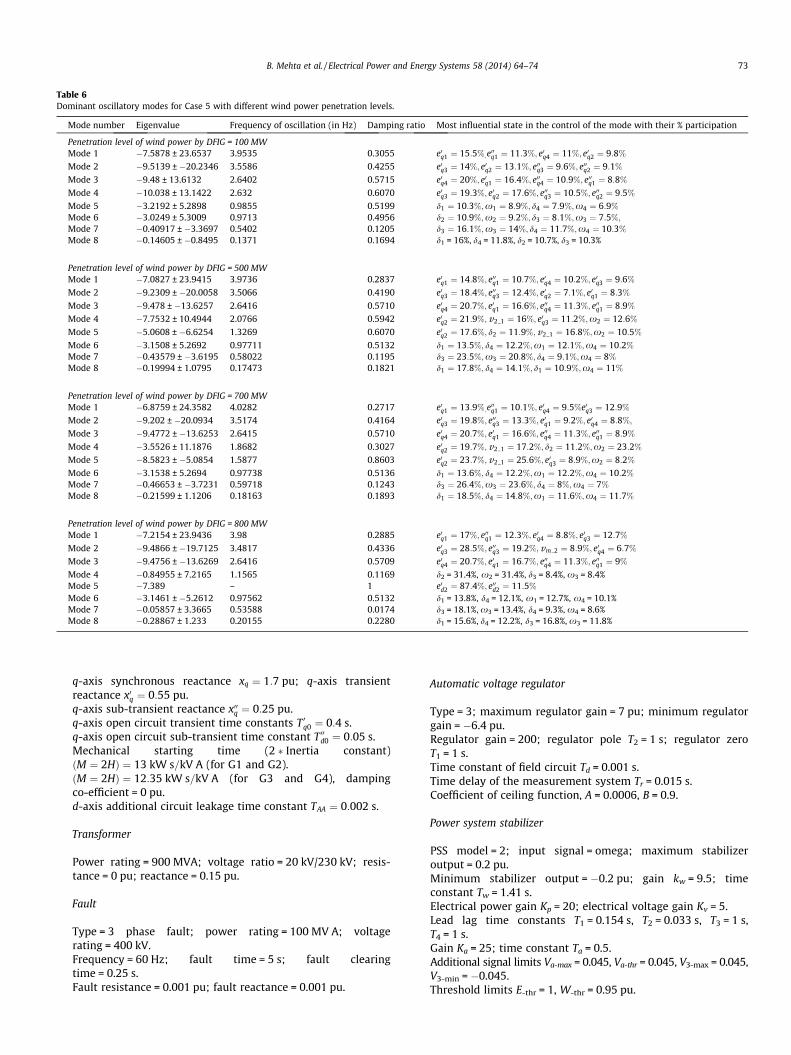
Table 6Dominant oscillatory modes for Case 5 with different wind power penetration levels.
Mode number Eigenvalue Frequency of oscillation (in Hz) Damping ratio Most influential state in the control of the mode with their % participation
Penetration level of wind power by DFIG = 100 MWMode 1 �7.5878 ± 23.6537 3.9535 0.3055 e0q1 ¼ 15:5%;e00q1 ¼ 11:3%; e0q4 ¼ 11%; e0q2 ¼ 9:8%
Mode 2 �9.5139 ± �20.2346 3.5586 0.4255 e0q3 ¼ 14%; e0q2 ¼ 13:1%; e00q3 ¼ 9:6%; e00q2 ¼ 9:1%
Mode 3 �9.48 ± 13.6132 2.6402 0.5715 e0q4 ¼ 20%; e0q1 ¼ 16:4%; e00q4 ¼ 10:9%; e00q1 ¼ 8:8%
Mode 4 �10.038 ± 13.1422 2.632 0.6070 e0q3 ¼ 19:3%; e0q2 ¼ 17:6%; e00q3 ¼ 10:5%; e00q2 ¼ 9:5%
Mode 5 �3.2192 ± 5.2898 0.9855 0.5199 d1 ¼ 10:3%;x1 ¼ 8:9%; d4 ¼ 7:9%;x4 ¼ 6:9%
Mode 6 �3.0249 ± 5.3009 0.9713 0.4956 d2 ¼ 10:9%;x2 ¼ 9:2%; d3 ¼ 8:1%;x3 ¼ 7:5%;
Mode 7 �0.40917 ± �3.3697 0.5402 0.1205 d3 ¼ 16:1%;x3 ¼ 14%; d4 ¼ 11:7%;x4 ¼ 10:3%
Mode 8 �0.14605 ± �0.8495 0.1371 0.1694 d1 = 16%, d4 = 11.8%, d2 = 10.7%, d3 = 10.3%
Penetration level of wind power by DFIG = 500 MWMode 1 �7.0827 ± 23.9415 3.9736 0.2837 e0q1 ¼ 14:8%; e00q1 ¼ 10:7%; e0q4 ¼ 10:2%; e0q3 ¼ 9:6%
Mode 2 �9.2309 ± �20.0058 3.5066 0.4190 e0q3 ¼ 18:4%; e00q3 ¼ 12:4%; e0q2 ¼ 7:1%; e0q1 ¼ 8:3%
Mode 3 �9.478 ± �13.6257 2.6416 0.5710 e0q4 ¼ 20:7%; e0q1 ¼ 16:6%; e00q4 ¼ 11:3%; e00q1 ¼ 8:9%
Mode 4 �7.7532 ± 10.4944 2.0766 0.5942 e0q2 ¼ 21:9%; v2 1 ¼ 16%; e0q3 ¼ 11:2%;x2 ¼ 12:6%
Mode 5 �5.0608 ± �6.6254 1.3269 0.6070 e0q2 ¼ 17:6%; d2 ¼ 11:9%;v2 1 ¼ 16:8%;x2 ¼ 10:5%
Mode 6 �3.1508 ± 5.2692 0.97711 0.5132 d1 ¼ 13:5%; d4 ¼ 12:2%;x1 ¼ 12:1%;x4 ¼ 10:2%
Mode 7 �0.43579 ± �3.6195 0.58022 0.1195 d3 ¼ 23:5%;x3 ¼ 20:8%; d4 ¼ 9:1%;x4 ¼ 8%
Mode 8 �0.19994 ± 1.0795 0.17473 0.1821 d1 ¼ 17:8%; d4 ¼ 14:1%; d1 ¼ 10:9%;x4 ¼ 11%
Penetration level of wind power by DFIG = 700 MWMode 1 �6.8759 ± 24.3582 4.0282 0.2717 e0q1 ¼ 13:9%;e00q1 ¼ 10:1%; e0q4 ¼ 9:5%e0q3 ¼ 12:9%
Mode 2 �9.202 ± �20.0934 3.5174 0.4164 e0q3 ¼ 19:8%; e00q3 ¼ 13:3%; e0q1 ¼ 9:2%; e0q4 ¼ 8:8%;
Mode 3 �9.4772 ± �13.6253 2.6415 0.5710 e0q4 ¼ 20:7%; e0q1 ¼ 16:6%; e00q4 ¼ 11:3%; e00q1 ¼ 8:9%
Mode 4 �3.5526 ± 11.1876 1.8682 0.3027 e0q2 ¼ 19:7%; v2 1 ¼ 17:2%; d2 ¼ 11:2%;x2 ¼ 23:2%
Mode 5 �8.5823 ± �5.0854 1.5877 0.8603 e0q2 ¼ 23:7%; v2 1 ¼ 25:6%; e0q3 ¼ 8:9%;x2 ¼ 8:2%
Mode 6 �3.1538 ± 5.2694 0.97738 0.5136 d1 ¼ 13:6%; d4 ¼ 12:2%;x1 ¼ 12:2%;x4 ¼ 10:2%
Mode 7 �0.46653 ± �3.7231 0.59718 0.1243 d3 ¼ 26:4%;x3 ¼ 23:6%; d4 ¼ 8%;x4 ¼ 7%
Mode 8 �0.21599 ± 1.1206 0.18163 0.1893 d1 ¼ 18:5%; d4 ¼ 14:8%;x1 ¼ 11:6%;x4 ¼ 11:7%
Penetration level of wind power by DFIG = 800 MWMode 1 �7.2154 ± 23.9436 3.98 0.2885 e0q1 ¼ 17%; e00q1 ¼ 12:3%; e0q4 ¼ 8:8%; e0q3 ¼ 12:7%
Mode 2 �9.4866 ± �19.7125 3.4817 0.4336 e0q3 ¼ 28:5%; e00q3 ¼ 19:2%; vm 2 ¼ 8:9%; e0q4 ¼ 6:7%
Mode 3 �9.4756 ± �13.6269 2.6416 0.5709 e0q4 ¼ 20:7%; e0q1 ¼ 16:7%; e00q4 ¼ 11:3%; e00q1 ¼ 9%
Mode 4 �0.84955 ± 7.2165 1.1565 0.1169 d2 = 31.4%, x2 = 31.4%, d3 = 8.4%, x3 = 8.4%Mode 5 �7.389 – 1 e0d2 ¼ 87:4%; e00d2 ¼ 11:5%
Mode 6 �3.1461 ± �5.2612 0.97562 0.5132 d1 = 13.8%, d4 = 12.1%, x1 = 12.7%, x4 = 10.1%Mode 7 �0.05857 ± 3.3665 0.53588 0.0174 d3 = 18.1%, x3 = 13.4%, d4 = 9.3%, x4 = 8.6%Mode 8 �0.28867 ± 1.233 0.20155 0.2280 d1 = 15.6%, d4 = 12.2%, d3 = 16.8%, x3 = 11.8%
B. Mehta et al. / Electrical Power and Energy Systems 58 (2014) 64–74 73
q-axis synchronous reactance xq ¼ 1:7 pu; q-axis transientreactance x0q ¼ 0:55 pu.q-axis sub-transient reactance x00q ¼ 0:25 pu.q-axis open circuit transient time constants T 0q0 ¼ 0:4 s.q-axis open circuit sub-transient time constant T 00d0 ¼ 0:05 s.Mechanical starting time (2 � Inertia constant)ðM ¼ 2HÞ ¼ 13 kW s=kV A (for G1 and G2).ðM ¼ 2HÞ ¼ 12:35 kW s=kV A (for G3 and G4), dampingco-efficient = 0 pu.d-axis additional circuit leakage time constant TAA ¼ 0:002 s.
Transformer
Power rating = 900 MVA; voltage ratio = 20 kV/230 kV; resis-tance = 0 pu; reactance = 0.15 pu.
Fault
Type = 3 phase fault; power rating = 100 MV A; voltagerating = 400 kV.Frequency = 60 Hz; fault time = 5 s; fault clearingtime = 0.25 s.Fault resistance = 0.001 pu; fault reactance = 0.001 pu.
Automatic voltage regulator
Type = 3; maximum regulator gain = 7 pu; minimum regulatorgain = �6.4 pu.Regulator gain = 200; regulator pole T2 = 1 s; regulator zeroT1 = 1 s.Time constant of field circuit Td = 0.001 s.Time delay of the measurement system Tr = 0.015 s.Coefficient of ceiling function, A = 0.0006, B = 0.9.
Power system stabilizer
PSS model = 2; input signal = omega; maximum stabilizeroutput = 0.2 pu.Minimum stabilizer output = �0.2 pu; gain kw = 9.5; timeconstant Tw = 1.41 s.Electrical power gain Kp = 20; electrical voltage gain Kv = 5.Lead lag time constants T1 = 0.154 s, T2 = 0.033 s, T3 = 1 s,T4 = 1 s.Gain Ka = 25; time constant Ta = 0.5.Additional signal limits Va-max = 0.045, Va-thr = 0.045, V3-max = 0.045,V3-min = �0.045.Threshold limits E-thr = 1, W-thr = 0.95 pu.
74 B. Mehta et al. / Electrical Power and Energy Systems 58 (2014) 64–74
Doubly fed induction generator
Power rating = (2 MV A � 450); voltage rating = 20 kV;frequency = 60 Hz.Stator resistance Rs = 0.01 pu; stator reactance Xs = 0.10 pu;rotor resistance Rr = 0.01 pu.Rotor reactance Xr = 0.08 pu; magnetization reactanceXm = 3 pu.Inertia constants, Hm = 3 kW s/kV A; pitch control gain = 10 pu;time constants = 3 s.Voltage control gain Kv = 10 pu; power control time constantTe = 0.01 s.Number of poles = 4; gear box ratio = 1:89; bladelength = 75.0 m; number of blade = 3.
References
[1] Global Wind Energy Council. Global wind energy outlook 2012 report. <http://www.gwec.net>.
[2] Muller S, Deicke M, De Doncker RW. Doubly fed induction generator systemsfor wind turbines. In: IEEE industrial application magazine; May/June, 2002.p. 26–33
[3] Xu Lie, Cartwright Phillip. Direct active and reactive power control of DFIG forwind energy generation. IEEE Trans Energy Convers 2006;21(3):750–8.
[4] Ekanayake JB, Holdsworth L, Wu X, Jenkins N. Dynamic modelling of doublyfed induction generator wind turbines. IEEE Trans Power Syst2003;18(2):803–9.
[5] Mei Francoise, Pal Bikash C. Modelling and small-signal analysis of a gridconnected doubly-fed induction generator. In: IEEE power engineering societygeneral meeting, vol. 3; June 2005. p. 2101–8
[6] Lei Y, Mullane A, Lightbody G, Yacamini R. Modeling of the wind turbine with adoubly fed induction generator for grid integration studies. IEEE Trans EnergyConvers 2006;21(1):257–64.
[7] Akhmatov V, Knudsen H. An aggregate model of a gridconnected, large-scale,offshore wind farm for power stability investigations-importance of windmillmechanical system. Elect Power Energy Syst 2002;24:709–17.
[8] Yang Lihui, Xu Zhao, Østergaard Jacob, Dong Zhao Yang, Wong Kit Po, Ma Xikui.Oscillatory stability and eigenvalue sensitivity analysis of a DFIG wind turbinesystem. IEEE Trans Energy Convers 2011;26(1):328–39.
[9] Thakur D, Mithulananthan N. Influence of constant speed wind turbinegenerator on power system oscillation. Elect Power Compon Syst2009;37:478–94.
[10] Gautam Durga, Goel Lalit, Ayyanar Raja, Vittal Vijay, Harbour Terry. Controlstrategy to mitigate the impact of reduced inertia due to doubly fed inductiongenerators on large power systems. IEEE Trans Power Syst 2011;26(1):214–24.
[11] Tsourakis G, Nomikos BM, Vournas CD. Effect of wind parks with doubly fedasynchronous generators on small signal stability. Elect Power Syst Res2009;79:190–200.
[12] Mishra Y, Mishra S, Li Fangxing. Coordinated tuning of DFIG-based windturbines and batteries using bacteria foraging technique for maintainingconstant grid power output. IEEE Syst J 2012;6(1):16–26.
[13] Mishra Y, Mishra S, Tripathy M, Senroy N, Dong ZY. Improving stability of aDFIG-based wind power system with tuned damping controller. IEEE TransEnergy Convers 2009;24(3):650–60.
[14] Guatam D, Vittal V, Harbour T. Impact of increased penetration of DFIG-basedwind turbine generators on transient and small signal stability of powersystems. IEEE Trans Power Syst 2009;24(3):1426–34.
[15] Meegahapola Lasantha Gunaruwan, Littler Tim, Flynn Damian. Decoupled-DFIG fault ride-through strategy for enhanced stability performance duringgrid faults. IEEE Trans Sust Energy 2010;1(3):152–62.
[16] Hagstrom E, Norheim I, Uhlen K. Large-scale wind power integration inNorway and impact on damping in the Nordic grid. Wind Energy J2005;8(3):375–84.
[17] Fernandez RD, Mantz RJ, Battaiotto PE. Impact of wind farms on a powersystem: an eigenvalue analysis approach. Renew Energy2007;32(10):1676–88.
[18] Mei F, Pal B. Modal analysis of grid-connected doubly fed induction generators.IEEE Trans Energy Convers 2007;22(3):728–36.
[19] Vittal V. Consequence and impact of electric utility industry restructuring ontransient stability and small-signal stability analysis. Proc IEEE2000;88(2):196–207.
[20] Attya AB, Hartkopf T. Penetration impact of wind farms equipped withfrequency variations ride through algorithm on power system frequencyresponse. Int J Elect Power Energy Syst 2012;40:94–103.
[21] Hughes FM, Anaya-Lara O, Jenkins N, Strbac G. Control of DFIG-based windgeneration for power network support. IEEE Trans Power Syst2005;20(4):1958–66.
[22] Krause PC, Wasynczuk O, Sudhoff SD. Analysis of electric machinery and drivesystems. 2nd ed.. John Wiley and Sons, Inc. Publication; 2002.
[23] Kundur P. Power system stability and control. The EPRI power systemengineering series. New York: McGraw-Hill Inc; 1994.
[24] Milano Federico. Power system analysis toolbox. PSAT version 2.1.6.[25] MATLAB help tutorial. The Math Works, Inc., version 7.8.0.347; 2009.[26] Ghosh Sudipta, Senroy Nilanjan. The localness of electromechanical
oscillations in power systems. Int J Elect Power Energy Syst 2012;42:306–13.[27] deMello FP, Concordia C. Concepts of synchronous machine stability as
effected by excitation control. IEEE Trans Power Appl Syst PAS1969;88:316–29.