Ministry of Education and Science of Ukraine

National Aerospace University n. a. N. E. Zhukovsky “Kharkiv Aviation Institute”

V. Sklyar, O. Illiashenko, V. Kharchenko, N. Zagorodna, R. Kozak, O. Vambol,

S. Lysenko, D. Medzatyi, O. Pomorova

SECURE AND RESILIENT COMPUTING FOR INDUSTRY AND HUMAN DOMAINS.

Fundamentals of security and resilient computing

Multi-book, Volume 1

V. S. Kharchenko eds.

Tempus project SEREIN 543968-TEMPUS-1-2013-1-EE-TEMPUS-JPCR

Modernization of Postgraduate Studies on Security and Resilience for Human and Industry Related Domains

2017

V. Sklyar, O. Illiashenko, V. Kharchenko, N. Zagorodna, R. Kozak, O. Vambol, S. Lysenko, D. Medzatyi, O. Pomorova. Secure and resilient computing for industry and human domains. Volume 1. Fundamentals of security and resilient computing / Edited by Kharchenko V. S. – Department of Education and Science of Ukraine, National Aerospace University named after N. E. Zhukovsky “KhAI”, 2017.

Reviewers: Dr. Peter Popov, Centre for Software Reliability, School of Informatics, City Universi-

ty of London Prof. Stefano Russo, Consorzio Interuniversitario Nazionale per l’Informatica (Na-

ples, Italy) Prof. Todor Tagarev, Centre for Security and Defence Management, Institute of In-

formation and Communication Technologies of the Bulgarian Academy of Sciences; Prof. Jüri Vain, School of Information Technologies, Department of Software Tallinn

University of Technology The first volume of the three volume book called “Secure and resilient computing

for industry and human domains” contains materials of the lecture parts of the study modules for MSc and PhD level of education as well as lecture part of in-service training modules developed in the framework of the SEREIN project "Modernization of Postgraduate Studies on Security Resilience for Human and Industry Related Domains"

1

(543968-TEMPUS-1-2013-1-EE-TEMPUS-JPCR) funded under the Tempus programme are given. The book material covers fundamentals issue of secure and resilient computing, in particular, description of related standards, methods of cryptography, software security assurance and post-quantum computing methods review.

The descriptions of trainings, which are intended for studying with technologies and means of assessing security guarantees, are given in accordance with international stand-ards and requirements. Courses syllabuses and description of practicums are placed in the correspondent notes on practicums and in-service training modules.

Designed for engineers who are currently or tend to design, develop and implement information security systems, for verification teams and professionals in the field of quali-ty assessment and assurance of cyber security of IT systems, for masters and PhD stu-dents from universities that study in the areas of information security, computer science, computer and software engineering, as well as for lecturers of the corresponding courses.

The materials in the book are given in a form “as is”, desktop publishing of this book is available in hard copy only. © V. Sklyar, O. Illiashenko, V. Kharchenko, N. Zagorodna, R. Kozak, O. Vambol, S. Lysenko, D. Medzatyi, O. Pomorova. 2017 This work is subject to copyright. All rights are reserved by the authors, whether the whole or part of the material is concerned, specifically the rights of translation, reprinting, reuse of illustrations, recitation, broadcasting, reproduction on microfilms, or in any other physical way, and transmission or information storage and retrieval, electronic adaptation, computer software, or by similar or dissimilar methodology now known or hereafter developed.

1 This project has been funded with support from the European Commission. This publication (com-

munication) reflects the views only of the author, and the Commission cannot be held responsible for any use which may be made of the information contained therein.

1 STANDARDS FOR SECURITY OF SAFETY CRITICAL SYSTEMS

1.1 Survey of standards in security At the present security standards are developed by many national

and international standardization organizations. The most relevant to safety critical systems are the following security standards sets:

– ISO/IEC 27000 “Information technology – Security techniques – Information security management systems” standards family states requirements to the Information Security Management System (ISMS) independently from type of computer system or organization; this series contains about 40 parts and is an umbrella document for all other documents in security (see Section 1.2);

– ISO/IEC 15408 “Information technology – Security techniques –Evaluation criteria for IT security” establishes Common Criteria to evaluate security functions and assurance techniques for information product (see Section 1.3) [1];

– ISA/IEC 62443 “Security for Industrial Automation and Control Systems” (see Section 1.4);

– The United States National Institute of Standards and Technology (NIST) developed NIST SP 800 series which cover many security issues; formally NIST standards are national but many countries and companies apply it as valuable state-of-the-art requirements; the NIST Cybersecurity Framework (SCF) based on NIST SP 800-53 “Security and Privacy Controls for Federal Information Systems and Organizations” is described in Section 1.5 [2,3];

– Institute of Electrical and Electronics Engineers (IEEE) standards, such as IEEE 1686-2007 “Standard for Substation Intelligent Electronic Devices IED Cybersecurity Capabilities”, IEEE P1711 “Standard for a Cryptographic Protocol for Cybersecurity of Substation Serial Links”, IEEE 1815-2012 “Standard for Electric Power System Communications-Distributed Network Protocol (DNP3)”;

– Standards applicable to specific domains which give details of the above standards requirements; we consider nuclear standard IEC 62645 “Nuclear power plants – Instrumentation and control

systems – Cybersecurity requirements” with associated IEC 62859 “Nuclear power plants – Instrumentation and control systems – Coordination between safety and cybersecurity” and IEC 62988 “Nuclear power plants – Instrumentation and control important to safety – Selection and use of wireless devices”.

Also it should be mentioned a lot of activities, performed in different industrial domains by technical and research organizations. The most powerful organizations are working in USA as a part of the continuing effort to provide effective security standards and guidance to federal agencies and their contractors in support of the Federal Information Security Management Act (FISMA). FISMA was signed into law part of the Electronic Government Act of 2002. There are the following organizations, addressing security [4]:

– The USA Department of Energy (DOE) developed the Cybersecurity Capability Maturity Model (C2M2) from the Electricity Subsector Cybersecurity Capability Maturity Model (ES-C2M2) by removing sector specific references and terminology. The ES-C2M2 was developed in support of a White House initiative led by the DOE, in partnership with the Department of Homeland Security (DHS), and in collaboration with private and public sector experts;

– The American Gas Association (AGA), representing energy utility organizations that deliver natural gas customers industries throughout the United States. The AGA 12 series of documents recommends practices designed to protect supervisory control and data acquisition (SCADA) communications against cyber incidents [5];

– The American Petroleum Institute represents members involved in all aspects of the oil and natural gas industry. API 1164 provides guidance to the operators of oil and natural gas pipeline systems for managing SCADA system integrity and security;

– The Industrial Control Systems Cyber Emergency Response Team (ICS-CERT) operates within the National Cybersecurity and Integration Center (NCCIC), a division of the Department of Homeland Security's Office of Cybersecurity and Communications (DHS CS&C). NCCIC/ICS-CERT is a key component of the DHS Strategy for Securing Control Systems. ICS-CERT works with the control systems community to ensure that recommended practices, which are made

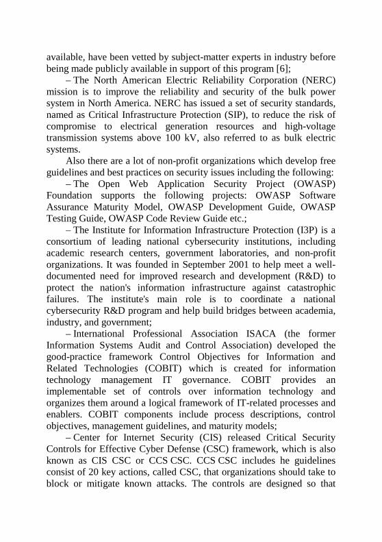
available, have been vetted by subject-matter experts in industry before being made publicly available in support of this program [6];

– The North American Electric Reliability Corporation (NERC) mission is to improve the reliability and security of the bulk power system in North America. NERC has issued a set of security standards, named as Critical Infrastructure Protection (SIP), to reduce the risk of compromise to electrical generation resources and high-voltage transmission systems above 100 kV, also referred to as bulk electric systems.

Also there are a lot of non-profit organizations which develop free guidelines and best practices on security issues including the following:

– The Open Web Application Security Project (OWASP) Foundation supports the following projects: OWASP Software Assurance Maturity Model, OWASP Development Guide, OWASP Testing Guide, OWASP Code Review Guide etc.;

– The Institute for Information Infrastructure Protection (I3P) is a consortium of leading national cybersecurity institutions, including academic research centers, government laboratories, and non-profit organizations. It was founded in September 2001 to help meet a well-documented need for improved research and development (R&D) to protect the nation's information infrastructure against catastrophic failures. The institute's main role is to coordinate a national cybersecurity R&D program and help build bridges between academia, industry, and government;

– International Professional Association ISACA (the former Information Systems Audit and Control Association) developed the good-practice framework Control Objectives for Information and Related Technologies (COBIT) which is created for information technology management IT governance. COBIT provides an implementable set of controls over information technology and organizes them around a logical framework of IT-related processes and enablers. COBIT components include process descriptions, control objectives, management guidelines, and maturity models;

– Center for Internet Security (CIS) released Critical Security Controls for Effective Cyber Defense (CSC) framework, which is also known as CIS CSC or CCS CSC. CCS CSC includes he guidelines consist of 20 key actions, called CSC, that organizations should take to block or mitigate known attacks. The controls are designed so that

primarily automated means can be used to implement, enforce and monitor them.

Taking into account variety of security standards, it should be noted they focus on some common issues. These issues include the following:

– Risk Management and Assessment [7]; – Information Security Management System [2,3]; – Security Life Cycle [8]; – Security Levels [4]; – Failures and attack avoidance [9,10]; – Security and safety relation for critical systems [4]. General security concept, directed to comprehensive security

assurance, is described in Part 4 of this multi-book. Below in this section a survey is done for the main security

standards, such as ISO/IEC 27000, ISA/IEC 62443, and NIST SP 800. 1.2 Standards family ISO/IEC 27000 ISO/IEC 27000 “Information technology – Security techniques–

Information security management systems” standards family contains about 40 parts and is an umbrella document for all other documents in security. Now many parts of ISO/IEC 27000 are booming, so many new parts are appearing and some existing parts are reworking once per 3-5 years.

The title standard in the family is ISO/IEC 27000:2016 “Information security management systems – Overview and vocabulary”.

All ISO/IEC 27000 standards family can be divided in the three following sets:

– Standards specifying requirements; – Standards describing general guidelines; – Standards describing sector-specific guidelines. Standards specifying requirements include the following: – ISO/IEC 27001 “Information security management systems –

Requirements” formally specifies ISMS against which thousands of organizations have been certified compliant;

– ISO/IEC 27006 “Requirements for bodies providing audit and certification of information security management systems” provides a

formal guidance for the for accredited organizations which certify other organizations compliant with ISO/IEC 27001;

– ISO/IEC 27009 “Sector-specific application of ISO/IEC 27001 – Requirements” at the time of 2016 is existing as a draft intended to provide guidance for those developing new ISO/IEC 27000 family standards.

Standards describing general guidelines include the following: – ISO/IEC 27002 “Code of practice for information security

controls” provides a reasonably comprehensive suite of information security control objectives and generally-accepted good practice security controls

– ISO/IEC 27003 “Information security management system implementation guidance” provides basic advices on implementing ISO/IEC 27001;

– ISO/IEC 27004 “Information security management – Measurement” provides description for a set of security metrics,

– ISO/IEC 27005 “Information security risk management” discusses risk management principles;

– ISO/IEC 27007 “Guidelines for information security management systems auditing” provides recommendations for auditing of management elements of the ISMS;

– ISO/IEC TR 27008 “Guidelines for auditors on information security management systems controls” provides recommendations for auditing the information security elements of the ISMS;

– ISO/IEC 27013 “Guidance on the integrated implementation of ISO/IEC 27001 and ISO/IEC 20000-1” combining ISO/IEC 27000 ISMS with ISO/IEC 20000 IT Service Management, particularly for ITIL (IT Infrastructure Library)

– ISO/IEC 27014 “Governance of information security” provide governing recommendations in the context of information security;

– ISO/IEC TR 27016 “Information security management – Organizational economics” provides economic theory applied to information security.

Standards describing sector-specific guidelines cover such domains as energy, medicine, telecommunications, finance, cloud computing and others.

For example, ISO/IEC 27010 “Information security management for inter-sector and inter-organisational communications” sharing

information on information security between industry sectors and/or nations, particularly those affecting “critical infrastructure”.

For more information concerning ISO/IEC 27000 see Part 9 of this multi-book.

1.3 Standards series ISO/IEC 15408 Standards series ISO/IEC 15408, which is also known as the

Common Criteria includes the following three parts: – ISO/IEC 15408-1 “Information technology – Security techniques

– Evaluation criteria for IT security – Part 1: Introduction and general model”;

– ISO/IEC 15408-2 “Information technology – Security techniques – Evaluation criteria for IT security – Part 2: Security functional components”;

– ISO/IEC 15408-3 “Information technology – Security techniques – Evaluation criteria for IT security – Part 2: Security assurance components”;

Part 1, “Introduction and general model” defines the general concepts and principles of IT security evaluation and presents a general model of evaluation (see Fig. 1.1). At the time evaluation concept is based on a confidence in correctness and sufficiency of security countermeasures (see Fig.1.2).

Part 2, “Security functional components” establishes a set of functional components that serve as standard templates upon which to base functional requirements for Targets of Evaluation (TOEs). ISO/IEC 15408-2 catalogues the set of functional components and organizes them in families and classes. There are the following classes of functional components described in ISO/IEC 15408-2: Security audit, Communication, Cryptographic support, User data protection, Identification and authentication, Security management, Privacy, Protection of the security functionality, Resource utilization, Access, Trusted path/channels.

Part 3, “Security assurance components” establishes a set of assurance components that serve as standard templates upon which to base assurance requirements for TOEs. ISO/IEC 15408-3 catalogues the set of assurance components and organizes them into families and classes. There are the following classes of assurance components

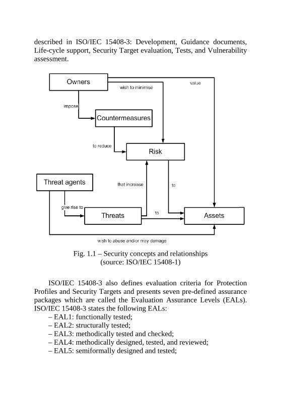
described in ISO/IEC 15408-3: Development, Guidance documents, Life-cycle support, Security Target evaluation, Tests, and Vulnerability assessment.

Fig. 1.1 – Security concepts and relationships

(source: ISO/IEC 15408-1)

ISO/IEC 15408-3 also defines evaluation criteria for Protection

Profiles and Security Targets and presents seven pre-defined assurance packages which are called the Evaluation Assurance Levels (EALs). ISO/IEC 15408-3 states the following EALs:

– EAL1: functionally tested; – EAL2: structurally tested; – EAL3: methodically tested and checked; – EAL4: methodically designed, tested, and reviewed; – EAL5: semiformally designed and tested;

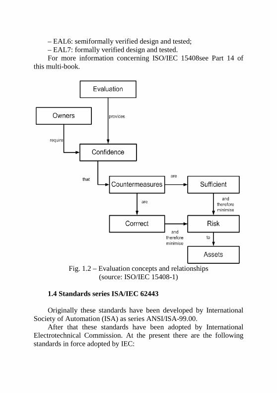
– EAL6: semiformally verified design and tested; – EAL7: formally verified design and tested. For more information concerning ISO/IEC 15408see Part 14 of

this multi-book.

Fig. 1.2 – Evaluation concepts and relationships

(source: ISO/IEC 15408-1) 1.4 Standards series ISA/IEC 62443 Originally these standards have been developed by International

Society of Automation (ISA) as series ANSI/ISA-99.00. After that these standards have been adopted by International

Electrotechnical Commission. At the present there are the following standards in force adopted by IEC:

– IEC TS 62443-1-1:2009 “Industrial communication networks – Network and system security – Part 1-1: Terminology, concepts and models”;

– IEC 62443-2-1:2010 “Industrial communication networks – Network and system security – Part 2-1: Establishing an industrial automation and control system security program”;

– IEC TR 62443-2-3:2015 “Security for industrial automation and control systems – Part 2-3: Patch management in the IACS environment”;

– IEC 62443-2-4:2015 “Security for industrial automation and control systems – Part 2-4: Security program requirements for IACS service providers”;

– IEC PAS 62443-3:2008 “Security for industrial process measurement and control – Network and system security”;

– IEC TR 62443-3-1:2009 “Industrial communication networks - Network and system security – Part 3-1: Security technologies for industrial automation and control systems”;

– IEC 62443-3-3:2013 “Industrial communication networks – Network and system security – Part 3-3: System security requirements and security levels”.

Now a structure of series is updated and new versions of the standards are in progress. ISA is developing master versions for the 62443 series, after that IEC should reissue identical standards. The developed 62443 series includes the following thirteen standards divided into four groups:

1) General: – ISA/IEC 62443-1-1 “Terminology, concepts and models”; – ISA/IEC 62443-1-2 “Master glossary of terms and

abbreviations”; – ISA/IEC 62443-1-3 “System security compliance metrics”; – ISA/IEC 62443-1-4 “Industrial Automation and Control Systems

(IACS) security lifecycle and use-case”; 2) Policies and Procedures: – ISA/IEC 62443-2-1 “Requirements for an IACS security

management system”; – ISA/IEC 62443-2-2 “Implementation guidance for an IACS

security management system”;

– ISA/IEC 62443-2-3 “Patch management in the IACS environment”;

– ISA/IEC 62443-2-4 “Installation and maintenance requirements for IACS suppliers”;

3) System: – ISA/IEC TR 62443-3-1 “Security techniques for IACS”; – ISA/IEC 62443-3-2 “Security levels for zones and conduits”; – ISA/IEC 62443-3-3 “System security requirements and security

levels”; 4) Component: – ISA/IEC 62443-4-1 “Product Development Requirements”; – ISA/IEC 62443-4-2 “Technical Security Requirements for IACS

Components”. The ISA/IEC 62443 series address the needs to design electronic

security robustness and resilience into industrial automation control systems (IACS). Robustness provides the capabilities for the IACS to operate under a range of cyber-induced perturbations and disturbances. Resilience provides the capabilities to restore the IACS after unexpected and rare cyber-induced events. Robustness and resilience are not general properties of IACS but are relevant to specific classes of cyber -induced perturbations. An IACS that is resilient or robust to a certain type of cyber-induced perturbations may be brittle or fragile to another. Such a trade-off is the subject of profiles, which others can derive from the ISA/IEC 62443 requirements and guidelines. The goal in developing the ISA/IEC 62443 series is to improve the availability, integrity and confidentiality of components or systems used for industrial automation and control, and to provide criteria for procuring and implementing secure industrial automation and control systems. Application of the requirements and guidance in ISA/IEC 62443 is intended to improve electronic security and help to reducing the risk of compromising confidential information or causing degradation or failure of the equipment (hardware and software) of systems under control. The concept of IACS electronic security is applied in the broadest possible sense, encompassing all types of plants, facilities, and systems in all industries. Automation and control systems include, but are not limited to:

– Hardware and software systems such as DCS, PLC, SCADA, networked electronic sensing, and monitoring and diagnostic systems;

– Associated internal, human, network, or machine interfaces used to provide control, safety, and manufacturing operations functionality to continuous, batch, discrete, and other processes.

The requirements and guidance are directed towards those responsible for designing, implementing, or managing IACS. This information also applies to users, system integrators, security practitioners, and control systems manufacturers and vendors.

For more information concerning security assurance approach as it is described in ISA/IEC 62443, see Part 4 of this multi-book.

1.5 National Institute of Standards and Technology

Cybersecurity Framework (NIST SCF) NIST SP 800-53 “Security and Privacy Controls for Federal

Information Systems and Organizations” provides a catalog of security controls measures. This catalog includes seventeen parts covering different organizational, technical and physical sides of security control (see Fig. 1.3).

Additionally NIST SP 800-53 it is a base for NIST CSF which harmonizes security control requirements with the following standards and good practices frameworks:

– ISO/IEC 27000 “Information security management systems” (see Section 1.2);

– ISA/IEC 62443 “Security for Industrial Automation and Control Systems”

– Control Objectives for Information and Related Technologies (COBIT) framework

– Center for Internet Security Critical Security Controls for Effective Cyber Defense framework (CIS CSC).

NIST CSF describes security activities by systematic way dividing into five the main functions: Identify, Protect, Detect, Respond, and Recover.

Each of the function is described through categories which include subcategories. Subcategories refer to Security Control Catalog (Appendix F of NIST SP 800-53), which provides a range of safeguards and countermeasures for organizations and information systems.

The following contains functions and categories description (see Fig. 1.4).

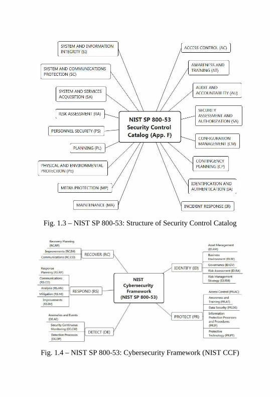
Fig. 1.3 – NIST SP 800-53: Structure of Security Control Catalog

Fig. 1.4 – NIST SP 800-53: Cybersecurity Framework (NIST CCF)

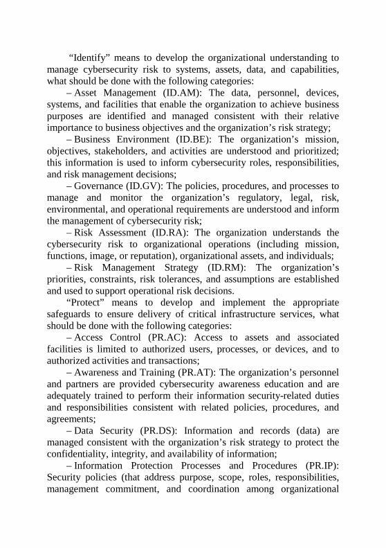
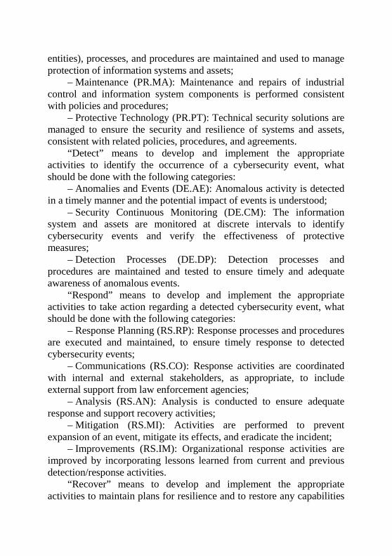
“Identify” means to develop the organizational understanding to manage cybersecurity risk to systems, assets, data, and capabilities, what should be done with the following categories:

– Asset Management (ID.AM): The data, personnel, devices, systems, and facilities that enable the organization to achieve business purposes are identified and managed consistent with their relative importance to business objectives and the organization’s risk strategy;

– Business Environment (ID.BE): The organization’s mission, objectives, stakeholders, and activities are understood and prioritized; this information is used to inform cybersecurity roles, responsibilities, and risk management decisions;

– Governance (ID.GV): The policies, procedures, and processes to manage and monitor the organization’s regulatory, legal, risk, environmental, and operational requirements are understood and inform the management of cybersecurity risk;

– Risk Assessment (ID.RA): The organization understands the cybersecurity risk to organizational operations (including mission, functions, image, or reputation), organizational assets, and individuals;

– Risk Management Strategy (ID.RM): The organization’s priorities, constraints, risk tolerances, and assumptions are established and used to support operational risk decisions.

“Protect” means to develop and implement the appropriate safeguards to ensure delivery of critical infrastructure services, what should be done with the following categories:

– Access Control (PR.AC): Access to assets and associated facilities is limited to authorized users, processes, or devices, and to authorized activities and transactions;

– Awareness and Training (PR.AT): The organization’s personnel and partners are provided cybersecurity awareness education and are adequately trained to perform their information security-related duties and responsibilities consistent with related policies, procedures, and agreements;

– Data Security (PR.DS): Information and records (data) are managed consistent with the organization’s risk strategy to protect the confidentiality, integrity, and availability of information;

– Information Protection Processes and Procedures (PR.IP): Security policies (that address purpose, scope, roles, responsibilities, management commitment, and coordination among organizational

entities), processes, and procedures are maintained and used to manage protection of information systems and assets;

– Maintenance (PR.MA): Maintenance and repairs of industrial control and information system components is performed consistent with policies and procedures;

– Protective Technology (PR.PT): Technical security solutions are managed to ensure the security and resilience of systems and assets, consistent with related policies, procedures, and agreements.

“Detect” means to develop and implement the appropriate activities to identify the occurrence of a cybersecurity event, what should be done with the following categories:

– Anomalies and Events (DE.AE): Anomalous activity is detected in a timely manner and the potential impact of events is understood;

– Security Continuous Monitoring (DE.CM): The information system and assets are monitored at discrete intervals to identify cybersecurity events and verify the effectiveness of protective measures;

– Detection Processes (DE.DP): Detection processes and procedures are maintained and tested to ensure timely and adequate awareness of anomalous events.

“Respond” means to develop and implement the appropriate activities to take action regarding a detected cybersecurity event, what should be done with the following categories:

– Response Planning (RS.RP): Response processes and procedures are executed and maintained, to ensure timely response to detected cybersecurity events;

– Communications (RS.CO): Response activities are coordinated with internal and external stakeholders, as appropriate, to include external support from law enforcement agencies;

– Analysis (RS.AN): Analysis is conducted to ensure adequate response and support recovery activities;

– Mitigation (RS.MI): Activities are performed to prevent expansion of an event, mitigate its effects, and eradicate the incident;

– Improvements (RS.IM): Organizational response activities are improved by incorporating lessons learned from current and previous detection/response activities.

“Recover” means to develop and implement the appropriate activities to maintain plans for resilience and to restore any capabilities

or services that were impaired due to a cybersecurity event, what should be done with the following categories:

– Recovery Planning (RC.RP): Recovery processes and procedures are executed and maintained to ensure timely restoration of systems or assets affected by cybersecurity events;

– Improvements (RC.IM): Recovery planning and processes are improved by incorporating lessons learned into future activities;

– Communications (RC.CO): Restoration activities are coordinated with internal and external parties, such as coordinating centers, Internet Service Providers, owners of attacking systems, victims, and vendors.

Conclusions There are a lot of dynamically developed standards in security

domain. Standards family ISO/IEC 27000 describes requirements to ISMS

which are implemented in many countries. All ISO/IEC 27000 standards family can be divided in the three following sets:

– Standards specifying requirements; – Standards describing general guidelines; – Standards describing sector-specific guidelines. However, many other standards and technical documents also

endorse ISMS with diverse interpretations. NIST SP 800 53 [2], for example, is used in USA to establish and assess ISMS. NIST CSF is harmonized with ISO/IEC 27000, as well as with ISA/IEC 62443, COBIT, and CIS CSC. NIST CSF describes security activities by systematic way dividing into five the main functions: Identify, Protect, Detect, Respond, and Recover.

At the same time, ISMS is mainly managerial and organizational issue, like Quality Management System or Project Management. ISMS describes processes which should be organized with under a concept of “Plan – Do – Check – Act” cycle. It means that for IT systems another part of requirements should be applied. Such requirements should also cover:

– Risk Management and Assessment [7]; – Security Life Cycle [8]; – Security Levels [4]; – Failures and attack avoidance [9,10];

– Security and safety relation for critical systems [4]. Standards series ISO/IEC 15408 endorse Common Criteria for IT

systems security assessment and provides security concepts including relations between basic security entities (risks, assets, threats, vulnerabilities, and countermeasures).

The most applicable requirements to Industrial Control Systems can be taken from NIST SP 800-82 [4] and ISA/IEC 62443 standards series.

Questions to self-checking 1. List a set of standards related with security issues. 2. List a set of organizations which develop security standards. 3. Which standards are more applicable for security of Industrial

Control Systems (ICS)? 4. Which standards are more applicable for security of web-

systems? 5. Which standards are more applicable for security of Internet

of Thing (IoT)? 6. Which main issues are covered in security standards? 7. Describe structure of ISO/IEC 27000 standards family. 8. Describe structure of ISO/IEC 15408 standards series. 9. What is a security concept stated in ISO/IEC 15408 standards

series? 10. Describe structure of ISA/IEC 62443 standards series. 11. Describe structure of NIST Cybersecurity Framework. 12. Which are the main issues of Security Management System? References 1. T. Nguyen, T. Levin, C. Irvine. High robustness requirements

in a Common Criteria protection profile // Proceeding of 2006 IEEE 4th International Workshop on Information Assurance (IWIA). – P.78-87.

2. NIST SP 800-53 Revision 4, Security and Privacy Controls for Federal Information Systems and Organizations. – National Institute of Standards and Technologies, 2015. – 462 p.

3. NIST SP 800-53A Revision 4, Assessing Security and Privacy Controls in Federal Information Systems and Organizations:

Building Effective Security Assessment Plans. – National Institute of Standards and Technologies, 2014. – 487 p.

4. NIST SP 800-82 Revision 2, Guide to Industrial Control Systems (ICS) Security: Supervisory Control and Data Acquisition (SCADA) Systems, Distributed Control Systems (DCS), and Other Control System Configurations such as Programmable Logic Controllers (PLC). – National Institute of Standards and Technologies, 2015. – 247 p.

5. AGA Report No. 12, Cryptographic Protection of SCADA Communications, Part 1: Background, Policies and Test Plan. – American Gas Association, 2006. – 123 p.

6. Common Cybersecurity Vulnerabilities in Industrial Control Systems. – U.S. Department of Homeland Security, 2011. – 76 p.

7. NIST SP 800-39, Managing Information Security Risk: Organization, Mission, and Information System View. – National Institute of Standards and Technologies, 2011. – 88 p.

8. Nuclear Power Plant Instrumentation and Control Systems for Safety and Security / Yastrebenetsky M., Kharchenko V. (Edits). – IGI Global. – 2014. – 470 p.

9. O. Netkachov, P. Popov, K. Salako. Model-Based Evaluation of the Resilience of Critical Infrastructures Under Cyber Attacks // Proceeding of 9th International Conference (CRITIS 2014). – P. 231-243.

10. S. Srinivasan, R. Kumar, J. Vain. Integration of IEC 61850 and OPC UA for Smart Grid automation // 2013 IEEE Innovative Smart Grid Technologies-Asia (ISGT Asia). – P. 1-5.

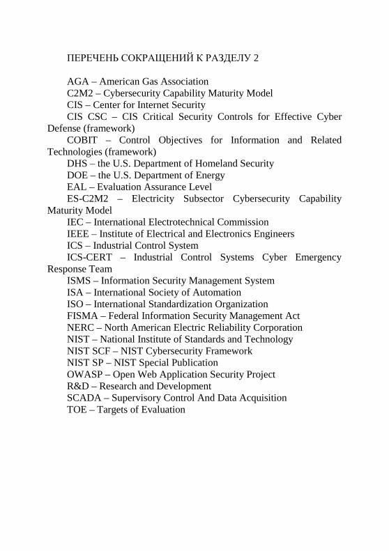
ПЕРЕЧЕНЬ СОКРАЩЕНИЙ К РАЗДЕЛУ 2 AGA – American Gas Association C2M2 – Cybersecurity Capability Maturity Model CIS – Center for Internet Security CIS CSC – CIS Critical Security Controls for Effective Cyber

Defense (framework) COBIT – Control Objectives for Information and Related

Technologies (framework) DHS – the U.S. Department of Homeland Security DOE – the U.S. Department of Energy EAL – Evaluation Assurance Level ES-C2M2 – Electricity Subsector Cybersecurity Capability

Maturity Model IEC – International Electrotechnical Commission IEEE – Institute of Electrical and Electronics Engineers ICS – Industrial Control System ICS-CERT – Industrial Control Systems Cyber Emergency

Response Team ISMS – Information Security Management System ISA – International Society of Automation ISO – International Standardization Organization FISMA – Federal Information Security Management Act NERC – North American Electric Reliability Corporation NIST – National Institute of Standards and Technology NIST SCF – NIST Cybersecurity Framework NIST SP – NIST Special Publication OWASP – Open Web Application Security Project R&D – Research and Development SCADA – Supervisory Control And Data Acquisition TOE – Targets of Evaluation

АННОТАЦИЯ В разделе рассмотрены стандарты в области информационной

безопасности. Приведен перечень основных существующих на данный момент стандартов. Дана характеристика наиболее важных стандартов (ISO/IEC 27000, ISO/IEC 15408, ISA/IEC 62443, NIST SP 800-53).

У розділі розглянуто стандарти у галузі інформаційної

безпеки. Наведено перелік основних існуючий у дійсний момент стандартів. Дана характеристика найбільш важливих стандартів (ISO/IEC 27000, ISO/IEC 15408, ISA/IEC 62443, NIST SP 800-53).

Information security standards are discussed in the section. List of

the main actual security standards is given. Contents of the most important security standards (ISO/IEC 27000, ISO/IEC 15408, ISA/IEC 62443, NIST SP 800-53) are considered.

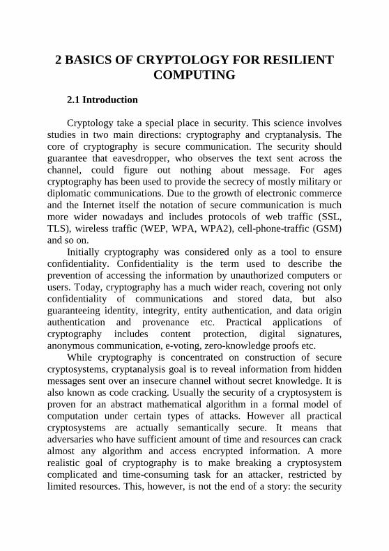
2 BASICS OF CRYPTOLOGY FOR RESILIENT COMPUTING

2.1 Introduction Cryptology take a special place in security. This science involves

studies in two main directions: cryptography and cryptanalysis. The core of cryptography is secure communication. The security should guarantee that eavesdropper, who observes the text sent across the channel, could figure out nothing about message. For ages cryptography has been used to provide the secrecy of mostly military or diplomatic communications. Due to the growth of electronic commerce and the Internet itself the notation of secure communication is much more wider nowadays and includes protocols of web traffic (SSL, TLS), wireless traffic (WEP, WPA, WPA2), cell-phone-traffic (GSM) and so on.

Initially cryptography was considered only as a tool to ensure confidentiality. Confidentiality is the term used to describe the prevention of accessing the information by unauthorized computers or users. Today, cryptography has a much wider reach, covering not only confidentiality of communications and stored data, but also guaranteeing identity, integrity, entity authentication, and data origin authentication and provenance etc. Practical applications of cryptography includes content protection, digital signatures, anonymous communication, e-voting, zero-knowledge proofs etc.

While cryptography is concentrated on construction of secure cryptosystems, cryptanalysis goal is to reveal information from hidden messages sent over an insecure channel without secret knowledge. It is also known as code cracking. Usually the security of a cryptosystem is proven for an abstract mathematical algorithm in a formal model of computation under certain types of attacks. However all practical cryptosystems are actually semantically secure. It means that adversaries who have sufficient amount of time and resources can crack almost any algorithm and access encrypted information. A more realistic goal of cryptography is to make breaking a cryptosystem complicated and time-consuming task for an attacker, restricted by limited resources. This, however, is not the end of a story: the security

must hold for the actual implementation of the algorithm in the real world in which this algorithm is run. A crucial difference about the two scenarios is that in the former we assume that secret keys are indeed secret, and the adversary has no information about them – our proofs crucially rely on this fact.

In reality cryptographic algorithms are routinely run in adversarial settings, where keys could be compromised and the adversary might gain some information about those secrets, by observing the behavior of the algorithm, in ways not captured by our formal computational model. Side-channel attacks exploit the fact that computing devices leak information to the outside world not just through input-output interaction, but through physical characteristics of computation such as power consumption, timing, and electro-magnetic radiation. Such information leakage betrays information about the secrets during cryptosystem execution, which cannot be efficiently derived from access to mathematical object alone. Physical attacks have been successfully utilized to break many cryptographic algorithms in common use. Attacks such as these have broken systems with a mathematical security proof, without violating any of the underlying mathematical principles. Physical leakages are particularly accessible when the device is at the hands of an adversary, as is often the case for modern devices such as smart-cards, TPM chips, mobile phones and laptops.

Leakage-resilient (or side-channel resilient) cryptography attempts to tackle such attacks. One main goal is building more robust models of adversarial access to a cryptographic algorithm, and developing methods grounded in modern cryptography to provably resist such attacks.

Although building efficient cryptosystem resilient to physical leakages and tampering people needs understanding the fundamentals of modern crypto-primitives.

2.2 Terminology. Classification of cryptosystems. Let clarify the terminology. Plaintext (message) is ordinary readable text before being

encrypted m = "𝑚𝑚1𝑚𝑚2𝑚𝑚3…𝑚𝑚𝑙𝑙"

where 𝑚𝑚𝑗𝑗 ∈ 𝐴𝐴𝑛𝑛, 𝑗𝑗 = 1. . 𝑙𝑙, An is an alphabet of n characters. Alphabet is a finite set of characters, which are used for

information coding. For instance, A26 could be a set of letters of English alphabet; A256 could be considered a set of symbols from ASCII table; A2={0,1} is a binary alphabet.

Ciphertext (23Tcyphertext23T) is encrypted plaintext: с = "𝑐𝑐1𝑐𝑐2𝑐𝑐3…𝑐𝑐𝑙𝑙",

where 𝑐𝑐𝑗𝑗 ∈ 𝐴𝐴𝑛𝑛, 𝑗𝑗 = 1. . 𝑙𝑙. Secret key is a parameter that is used to encrypt and decrypt

messages: k = "k

1

𝑘𝑘2𝑘𝑘3 … 𝑘𝑘𝑙𝑙", 𝑘𝑘𝑗𝑗 ∈ 𝐴𝐴𝑛𝑛, 𝑗𝑗 = 1. . 𝑙𝑙. Encryption is a process of conversion of information (plaintext)

into another form (ciphertext), which cannot be easily understood by anyone except owner of secret key.

Decryption is the reverse process to encryption conversion of ciphertext into plaintext with the secret key.

The simplest encryption methods date back to 2000-3000 BC when the ancient Greeks and Romans sent secret messages by substituting or permutation letters. There is a sufficiently large number of transposition ciphers. Among them are a Scytale cipher, anagrams, and variety of so called route ciphers: rail fence, columnar transposition, double transposition, Myszkowski transposition, Cardan grille. The main idea of all of them is change the location of symbols in plaintext according to some predefined permutation rules. There were much more substitution ciphers, which are based on substitution of plaintext symbol by symbol of ciphertext. They could be subdivided on two large groups: monoalphabetic ciphers (Polybius square, Caesar cipher, affine cipher, Trithemius cipher) and polyalphabetic ciphers (bigram affine cipher, Playfair cipher, hill cipher, Vigenère cipher). The difference is that in monoalphabetic ciphers fixed symbol of plaintext is substituted with the same symbol of ciphertext. In polyalphabetic ciphers same symbol can be replaced with different symbols depends on its position in the plaintext.

Symmetric encryption was the only type of encryption in use from the ancient till 1970s. Symmetric encryption transforms plaintext into ciphertext using a secret key and an encryption algorithm. Using the same key and a decryption algorithm, the plaintext is recovered from

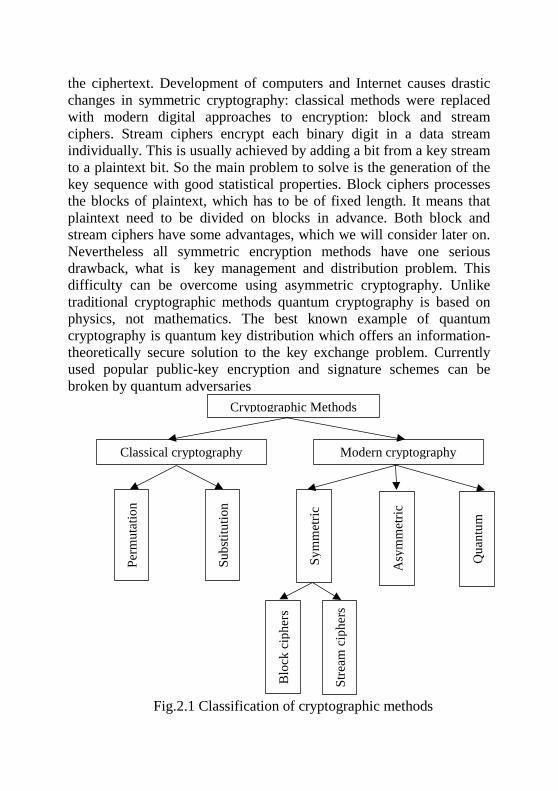
the ciphertext. Development of computers and Internet causes drastic changes in symmetric cryptography: classical methods were replaced with modern digital approaches to encryption: block and stream ciphers. Stream ciphers encrypt each binary digit in a data stream individually. This is usually achieved by adding a bit from a key stream to a plaintext bit. So the main problem to solve is the generation of the key sequence with good statistical properties. Block ciphers processes the blocks of plaintext, which has to be of fixed length. It means that plaintext need to be divided on blocks in advance. Both block and stream ciphers have some advantages, which we will consider later on. Nevertheless all symmetric encryption methods have one serious drawback, what is key management and distribution problem. This difficulty can be overcome using asymmetric cryptography. Unlike traditional cryptographic methods quantum cryptography is based on physics, not mathematics. The best known example of quantum cryptography is quantum key distribution which offers an information-theoretically secure solution to the key exchange problem. Currently used popular public-key encryption and signature schemes can be broken by quantum adversaries

Fig.2.1 Classification of cryptographic methods

Cryptographic Methods

Classical cryptography Modern cryptography

Perm

utat

ion

Subs

titut

ion

Sym

met

ric

Asy

mm

etric

Qua

ntum

Blo

ck c

iphe

rs

Stre

am c

iphe

rs

Which cryptographic methods are the best? Does there exist a

perfect cipher? Let clarify these questions further. 2.3 Perfect and computational secrecy There is a critical difference between the decryption performed by

the legitimate user and cryptanalysis performed by unauthorized person. Features and capabilities of potential attacker determine the requirements for reliable encryption. One of the key steps in the development of the secrecy model of cryptosystem is to define threat model and security goal.

Recall that the main goal of cryptanalysis is to restore the plaintext without knowledge of the key or to recover the secret key.

As a basic starting point it is normally assumed that, for the purposes of cryptanalysis, the general algorithm is known (Kerckhoffs' principle).

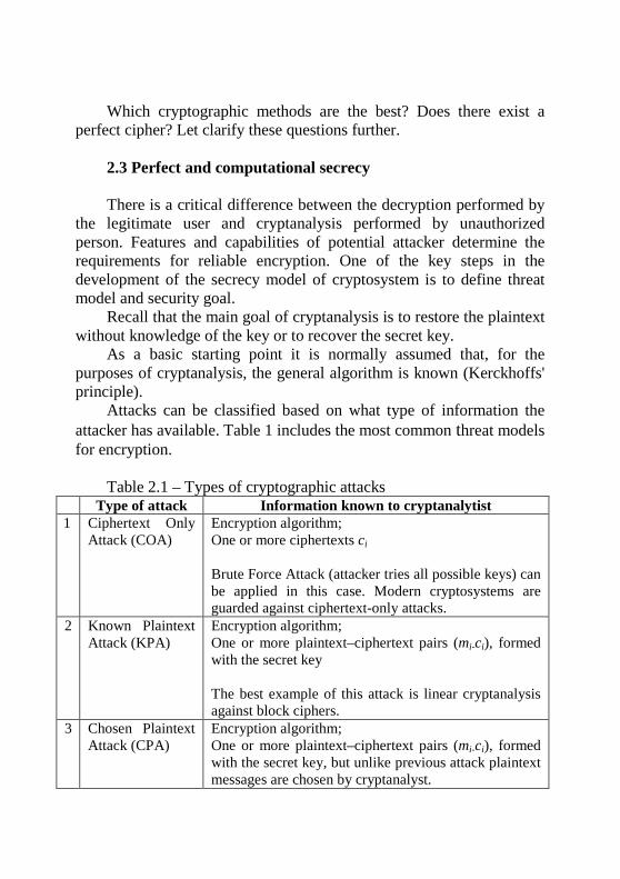
Attacks can be classified based on what type of information the attacker has available. Table 1 includes the most common threat models for encryption.

Table 2.1 – Types of cryptographic attacks

Type of attack Information known to cryptanalytist 1 Ciphertext Only

Attack (COA) Encryption algorithm; One or more ciphertexts ci Brute Force Attack (attacker tries all possible keys) can be applied in this case. Modern cryptosystems are guarded against ciphertext-only attacks.

2 Known Plaintext Attack (KPA)

Encryption algorithm; One or more plaintext–ciphertext pairs (mi-ci), formed with the secret key The best example of this attack is linear cryptanalysis against block ciphers.

3 Chosen Plaintext Attack (CPA)

Encryption algorithm; One or more plaintext–ciphertext pairs (mi-ci), formed with the secret key, but unlike previous attack plaintext messages are chosen by cryptanalyst.

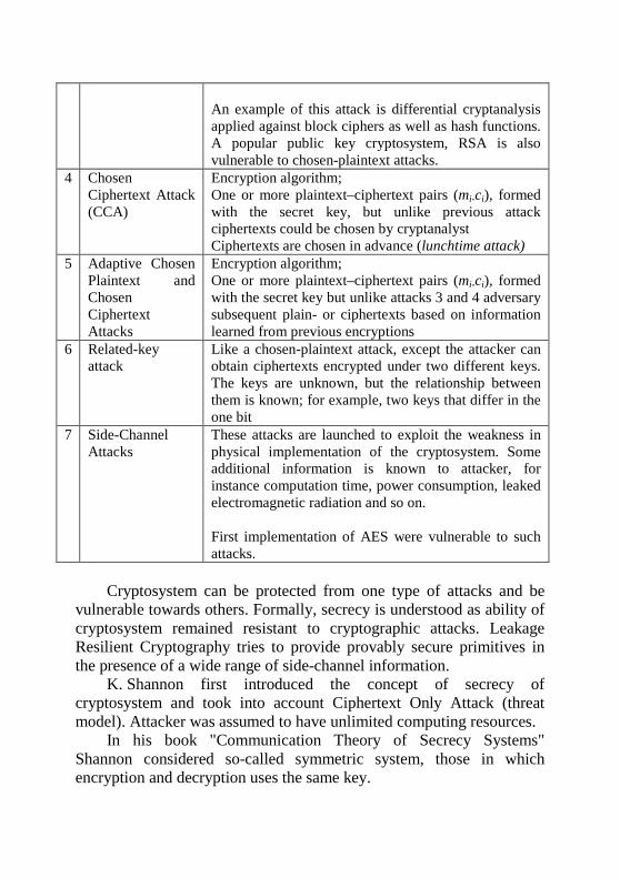
An example of this attack is differential cryptanalysis applied against block ciphers as well as hash functions. A popular public key cryptosystem, RSA is also vulnerable to chosen-plaintext attacks.

4 Chosen Ciphertext Attack (CCA)

Encryption algorithm; One or more plaintext–ciphertext pairs (mi-ci), formed with the secret key, but unlike previous attack ciphertexts could be chosen by cryptanalyst Ciphertexts are chosen in advance (lunchtime attack)

5 Adaptive Chosen Plaintext and Chosen Ciphertext Attacks

Encryption algorithm; One or more plaintext–ciphertext pairs (mi-ci), formed with the secret key but unlike attacks 3 and 4 adversary subsequent plain- or ciphertexts based on information learned from previous encryptions

6 Related-key attack

Like a chosen-plaintext attack, except the attacker can obtain ciphertexts encrypted under two different keys. The keys are unknown, but the relationship between them is known; for example, two keys that differ in the one bit

7 Side-Channel Attacks

These attacks are launched to exploit the weakness in physical implementation of the cryptosystem. Some additional information is known to attacker, for instance computation time, power consumption, leaked electromagnetic radiation and so on. First implementation of AES were vulnerable to such attacks.

Cryptosystem can be protected from one type of attacks and be

vulnerable towards others. Formally, secrecy is understood as ability of cryptosystem remained resistant to cryptographic attacks. Leakage Resilient Cryptography tries to provide provably secure primitives in the presence of a wide range of side-channel information.

K. Shannon first introduced the concept of secrecy of cryptosystem and took into account Ciphertext Only Attack (threat model). Attacker was assumed to have unlimited computing resources.

In his book "Communication Theory of Secrecy Systems" Shannon considered so-called symmetric system, those in which encryption and decryption uses the same key.

A symmetric (private-key) cryptosystem defined over (M,K,C) can be described in mathematical terms as a pair of “efficient” algorithms (Enc,Dec), such that:

– 𝐸𝐸𝑛𝑛𝑐𝑐: M×K→C – (encryption algorithm): takes key kϵK and message mϵM as inputs; outputs ciphertext c =Enc(k,m).

– 𝐷𝐷𝑒𝑒𝑐𝑐: C×K→M – (decryption algorithm): takes key kϵK and ciphertext cϵC as input; outputs message m=Dec(k,c), such that ∀k∈K and m∈M it is valid that Enc(k,Dec(k,m))=m (consistency equation).

Here: M – message space; K– key space; С – ciphertext space. Algorithm Enc could often a randomized algorithm. On the other

hand the decrypting algorithm Dec is always deterministic Often the pair (Enc, Dec) can be supplemented with one more

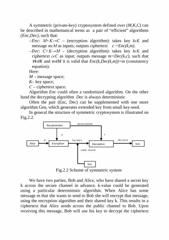
algorithm Gen, which generates extended key from small key-seed. In general the structure of symmetric cryptosystem is illustrated on

Fig.2.2.

Fig.2.2 Scheme of symmetric system We have two parties, Bob and Alice, who have shared a secret key

k across the secure channel in advance. k-value could be generated using a particular deterministic algorithm. When Alice has some message m that she wants to send to Bob she will encrypt that message, using the encryption algorithm and their shared key k. This results in a ciphertext that Alice sends across the public channel to Bob. Upon receiving this message, Bob will use his key to decrypt the ciphertext

Key generator

Alice Encryption m

k

Decryption Enc (m)=c

k

Secure channel

public channel

Bob Dec (c)=m

Eva

and recover the original message. At a high level, both parties are trying to ensure secrecy of their communication against an eavesdropper Eva who can observe everything being sent across the public channel between Alice and Bob.

Shannon believed that attacker would not be interested only in getting the entire secret message or key but also in some additional information about plaintext. The system has perfect secrecy by Shannon if regardless of any prior info the attacker has about the plaintext, the ciphertext should leak no additional information about the plaintext.

Besides the assumption that Ciphertext Only Attack is only possible attack and only one ciphertext is available scientist assumed that knows the probability distributions of messages P(M) and keys P(K).

Encryption scheme (Enc, Dec) with message space M, key space K and ciphertext space C is perfectly secret if for every distribution over M, every mϵM, and every cϵC with P(c)>0, it holds that

P(m│c)=P(m) So perfect secrecy means that observing the ciphertext should not

change the attacker’s knowledge about the distribution of the plaintext. Equivalent definition of perfect security could be formulated in

terms of entropy. For ∀m∈M,c∈C H(m│c)=H(m) It can treated as follows: attacker gets zero information from

ciphertext about plaintext 𝐼𝐼 = 𝐻𝐻(𝑚𝑚) − 𝐻𝐻(𝑚𝑚|𝑐𝑐) = 0. Shannon also proved the validity of few lemmas, which are based

on definition of perfect secrecy. Lemma 2.1. Cryptosystem has perfect secrecy if ∀m∈M, c∈C the equilaty:

P(c│m)=P(c) is valid.

Lemma 2.2. Cryptosystem with perfect secrecy will satisfy the inequality

#K≥#C≥#M This lemma is carrying bad news, because the total number of keys

has to be at least not less the number of messages. Shannon also gave the instructions how to construct the ideal system in next lemma.

Lemma 2.3.

If ⟨M,C,K, Enc(k,∙),Dec(k,∙)⟩ describes a particular symmetric cryptosystem and #K=#C=#M, it will have perfect secrecy only and only if

– The distribution of keys is uniform P(k)=1/(#K) for ∀k∈K – There is only one k∈K for each pair m∈M, c∈C such that

Enc(k,m)=c. The question is: Does the ideal system exist? It turns out the

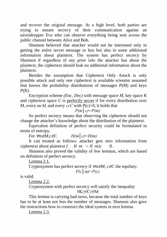
answer is “Yes” Gilbert Vernam invented and patented his cipher called also One-

time pad (OTP) in 1917. Let consider some details of algorithm Message space M={0,1}n is a set of all possible n-length bit

strings. Key is selected randomly on uniformly distributed set 𝐾𝐾 ={0,1}𝑛𝑛.

Encryption: ci=mi⨁ki (⨁ is a bit-wise XOR) Decryption: mi=ci⨁ki Illustration of OTP encryption scheme is depicted in Fig.2.3.

Fig.2.3 The encryption algorithm of OTP Shannon has also proven the following lemma. Lemma 2.4. Vernam cipher has perfect secrecy. Despite of the fact that OTP cipher is ideal it is hard to use it in

practice. Drawbacks of the practical usage of the OTP cipher: – Key has to be as long as message. – Key has to used only once Problem arisen if key is used more than once – In worst case chosen plaintext attack k = m ⊕ c

key

n bits

message

n bits

ciphertext

n bits

⊕

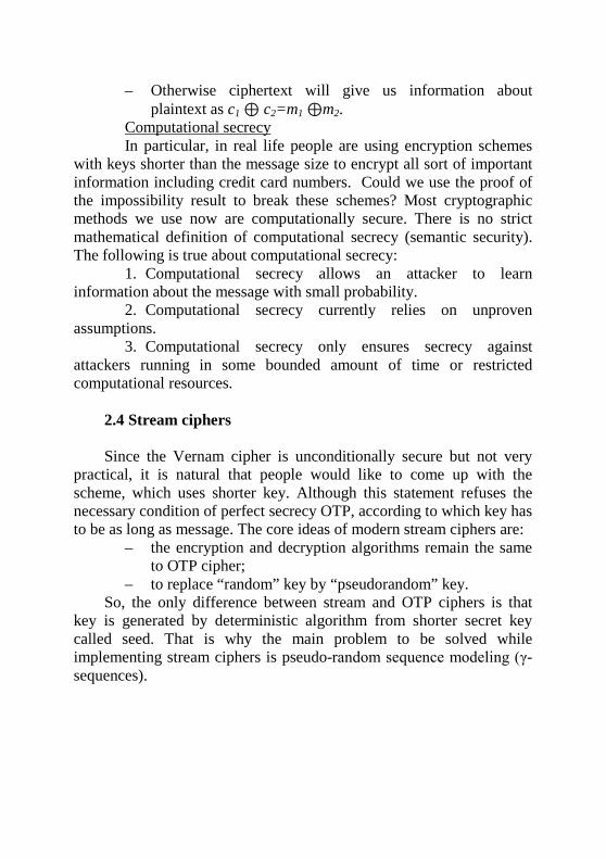
– Otherwise ciphertext will give us information about plaintext as c1 ⊕ c2=m1 ⊕m2.

Computational secrecy In particular, in real life people are using encryption schemes

with keys shorter than the message size to encrypt all sort of important information including credit card numbers. Could we use the proof of the impossibility result to break these schemes? Most cryptographic methods we use now are computationally secure. There is no strict mathematical definition of computational secrecy (semantic security). The following is true about computational secrecy:

1. Computational secrecy allows an attacker to learn information about the message with small probability.

2. Computational secrecy currently relies on unproven assumptions.

3. Computational secrecy only ensures secrecy against attackers running in some bounded amount of time or restricted computational resources.

2.4 Stream ciphers Since the Vernam cipher is unconditionally secure but not very

practical, it is natural that people would like to come up with the scheme, which uses shorter key. Although this statement refuses the necessary condition of perfect secrecy OTP, according to which key has to be as long as message. The core ideas of modern stream ciphers are:

– the encryption and decryption algorithms remain the same to OTP cipher;

– to replace “random” key by “pseudorandom” key. So, the only difference between stream and OTP ciphers is that

key is generated by deterministic algorithm from shorter secret key called seed. That is why the main problem to be solved while implementing stream ciphers is pseudo-random sequence modeling (γ- sequences).

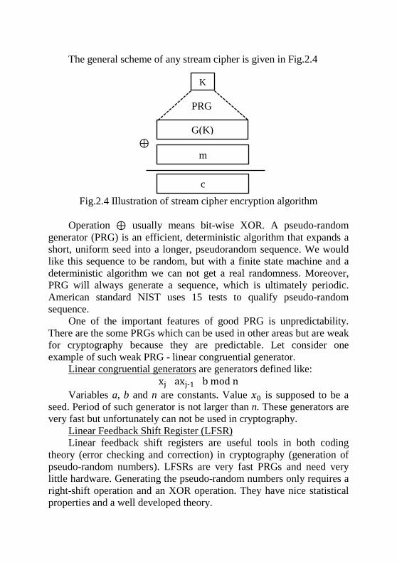
The general scheme of any stream cipher is given in Fig.2.4

Fig.2.4 Illustration of stream cipher encryption algorithm Operation ⊕ usually means bit-wise XOR. A pseudo-random

generator (PRG) is an efficient, deterministic algorithm that expands a short, uniform seed into a longer, pseudorandom sequence. We would like this sequence to be random, but with a finite state machine and a deterministic algorithm we can not get a real randomness. Moreover, PRG will always generate a sequence, which is ultimately periodic. American standard NIST uses 15 tests to qualify pseudo-random sequence.

One of the important features of good PRG is unpredictability. There are the some PRGs which can be used in other areas but are weak for cryptography because they are predictable. Let consider one example of such weak PRG - linear congruential generator.

Linear congruential generators are generators defined like: xj=axj-1+b mod n

Variables a, b and n are constants. Value 𝑥𝑥0 is supposed to be a seed. Period of such generator is not larger than n. These generators are very fast but unfortunately can not be used in cryptography.

Linear Feedback Shift Register (LFSR) Linear feedback shift registers are useful tools in both coding

theory (error checking and correction) in cryptography (generation of pseudo-random numbers). LFSRs are very fast PRGs and need very little hardware. Generating the pseudo-random numbers only requires a right-shift operation and an XOR operation. They have nice statistical properties and a well developed theory.

PRG

K

G(K)

m

c

⊕

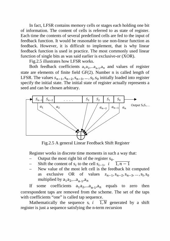
In fact, LFSR contains memory cells or stages each holding one bit of information. The content of cells is referred to as state of register. Each time the contents of several predefined cells are fed to the input of feedback function. It would be reasonable to use non-linear function as feedback. However, it is difficult to implement, that is why linear feedback function is used in practice. The most commonly used linear function of single bits as was said earlier is exclusive-or (XOR).

Fig.2.5 illustrates how LFSR works. Both feedback coefficients a1a2,…an-1,an and values of register

state are elements of finite field GF(2). Number n is called length of LFSR. The values 𝑠𝑠𝑛𝑛−1, sn−2, sn−3, … , sl, s0 initially loaded into register specify the initial state. The initial state of register actually represents a seed and can be chosen arbitrary.

Fig.2.5 A general Linear Feedback Shift Register Register works in discrete time moments in such a way that: – Output the most right bit of the register s0. – Shift the content of s𝑖𝑖 to the cell s𝑖𝑖−1, 𝑖𝑖 = 1, 𝑛𝑛 − 1���������� – New value of the most left cell is the feedback bit computed

as exclusive OR of values 𝑠𝑠𝑛𝑛−1, sn−2, sn−3, … , sl, s0 multiplied by a1a2,…an-1,an

If some coefficients a1a2,…an-1,an equals to zero then correspondent taps are removed from the scheme. The set of the taps with coefficients “one” is called tap sequence.

Mathematically the sequence si 𝑖𝑖 = 1, 𝑁𝑁����� generated by a shift register is just a sequence satisfying the n-term recursion

𝑎𝑎1

𝑎𝑎𝑛𝑛

𝑎𝑎𝑛𝑛−1

𝑎𝑎𝑛𝑛−2

𝑎𝑎2

𝑆𝑆𝑛𝑛−1

𝑆𝑆𝑛𝑛−2

. . . . 𝑆𝑆3

𝑆𝑆2

𝑆𝑆1

𝑆𝑆0

Output S0S1…

sn+t=a1sn+t-1⨁a2sn+t-2⨁…⨁an-2st+2⨁an-1st+1⨁anst= � aj

n

j=1

sn+t-j

The last formula describes the feedback function. It is called the recursion law which generate the sequence.

Output sequence of LFSR can be uniquely defined by feedback polynomial and initial state of register.

LFSR of length n with coefficients a1a2,…an-1,an has feedback polynomial:

P(x)=1⨁ � ai

n

j=1

xi=xn⨁a1x⨁a2x2⨁…⨁an-1xn-1⨁anxn

Alternatively register output can be defined by characteristic polynomial of LFSR.

P*(x)=xn⨁ � ajxn-jn

j=1

=xn⨁a1xn-1⨁a2xn-2⨁…⨁an-1x⨁an

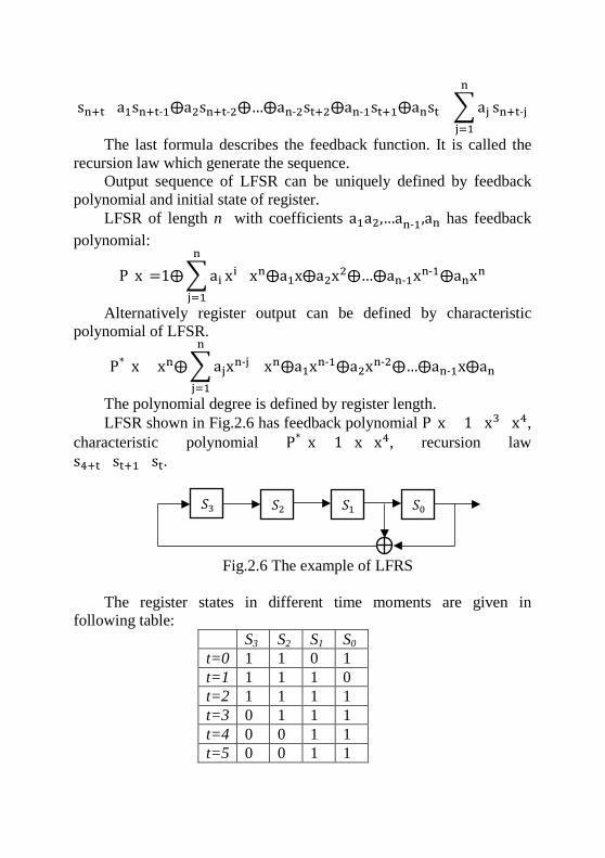
The polynomial degree is defined by register length. LFSR shown in Fig.2.6 has feedback polynomial P(x)=1+x3+x4,

characteristic polynomial P*(x)=1+x+x4, recursion law s4+t=st+1+st.

Fig.2.6 The example of LFRS The register states in different time moments are given in

following table: S3 S2 S1 S0 t=0 1 1 0 1 t=1 1 1 1 0 t=2 1 1 1 1 t=3 0 1 1 1 t=4 0 0 1 1 t=5 0 0 1 1

𝑆𝑆3

𝑆𝑆2

𝑆𝑆1

𝑆𝑆0

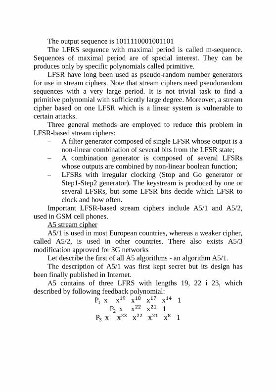
The output sequence is 1011110001001101 The LFRS sequence with maximal period is called m-sequence.

Sequences of maximal period are of special interest. They can be produces only by specific polynomials called primitive.

LFSR have long been used as pseudo-random number generators for use in stream ciphers. Note that stream ciphers need pseudorandom sequences with a very large period. It is not trivial task to find a primitive polynomial with sufficiently large degree. Moreover, a stream cipher based on one LFSR which is a linear system is vulnerable to certain attacks.

Three general methods are employed to reduce this problem in LFSR-based stream ciphers:

– A filter generator composed of single LFSR whose output is a non-linear combination of several bits from the LFSR state;

– A combination generator is composed of several LFSRs whose outputs are combined by non-linear boolean function;

– LFSRs with irregular clocking (Stop and Go generator or Step1-Step2 generator). The keystream is produced by one or several LFSRs, but some LFSR bits decide which LFSR to clock and how often.

Important LFSR-based stream ciphers include A5/1 and A5/2, used in GSM cell phones.

A5 stream cipher A5/1 is used in most European countries, whereas a weaker cipher,

called A5/2, is used in other countries. There also exists A5/3 modification approved for 3G networks

Let describe the first of all A5 algorithms - an algorithm A5/1. The description of A5/1 was first kept secret but its design has

been finally published in Internet. А5 contains of three LFRS with lengths 19, 22 і 23, which

described by following feedback polynomial: P1(x)=x19+x18+x17+x14+1

P2(x)=x22+x21+1 P3(x)=x23+x22+x21+x8+1

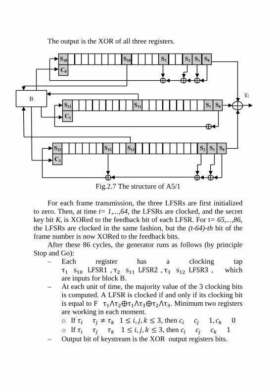
The output is the XOR of all three registers.

Fig.2.7 The structure of A5/1

For each frame transmission, the three LFSRs are first initialized to zero. Then, at time t= 1,...,64, the LFSRs are clocked, and the secret key bit Kt is XORed to the feedback bit of each LFSR. For t= 65,...,86, the LFSRs are clocked in the same fashion, but the (t-64)-th bit of the frame number is now XORed to the feedback bits.

After these 86 cycles, the generator runs as follows (by principle Stop and Go):

– Each register has a clocking tap τ1=s10 (LFSR1), τ2=s11(LFSR2), τ3=s12(LFSR3), which are inputs for block B.

– At each unit of time, the majority value of the 3 clocking bits is computed. A LFSR is clocked if and only if its clocking bit is equal to F=τ1⋀τ2⨁τ1⋀τ3⨁τ2⋀τ3. Minimum two registers are working in each moment. o If 𝜏𝜏𝑖𝑖 = 𝜏𝜏𝑗𝑗 ≠ 𝜏𝜏𝑘𝑘 1 ≤ 𝑖𝑖, 𝑗𝑗, 𝑘𝑘 ≤ 3, then 𝑐𝑐𝑖𝑖 = 𝑐𝑐𝑗𝑗 = 1, 𝑐𝑐𝑘𝑘 = 0 o If 𝜏𝜏𝑖𝑖 = 𝜏𝜏𝑗𝑗 = 𝜏𝜏𝑘𝑘 1 ≤ 𝑖𝑖, 𝑗𝑗, 𝑘𝑘 ≤ 3, then 𝑐𝑐𝑖𝑖 = 𝑐𝑐𝑗𝑗 = 𝑐𝑐𝑘𝑘 = 1

– Output bit of keystream is the XOR output registers bits.

ɣ𝑖𝑖 B

S0 S1 S2 S5 S10 S18

С0

S0 S1 S11 S21

С1

S0 S1 S12 S22

С3

S2 S15

Famous cryptanalyst at Cambridge Ian Cassells said “Cryptography is a mixture of mathematics and muddle, and without the muddle mathematics can be used against you” He meant that to study and to proof the secrecy of ciphers we need to base on strong mathematical structures. At the same time to make ciphers stronger to attacks we need to add nonlinear muddle. This is true with respect to both stream and block ciphers.

2.5 Block ciphers Stream ciphers are much faster than their closest competitors -

block ciphers but only in the case if stream encryption is implemented in hardware. Block ciphers are easier to implement in software, since we can avoid significant manipulation of bits and operate data blocks which are more convenient for computers.

DES (Data Encryption Standard) In 1974 the National Bureau of Standards (NBS) solicited the

American industry to develop a cryptosystem that could be used as a standard in unclassified U.S. Government applications. IBM developed a system called LUCIFER. NBS involved National Security Agency (NSA) to review and assess this cipher. After being modified and simplified during review time, this system became the Data Encryption Standard (DES) in 1977.

DES parameters: – Length of plaintext and ciphertext block is 64 bits. – Key length is 64 bits, but the least significant bit of each key

byte is used for parity check and could be ignored. Effective keysize is 56 bits

– Number of rounds is 16. DES is an example of a Feistel cipher. Horst Feistel was one of the

inventors of cipher LUCIFER – DES predecessor. A Feistel network works by splitting the data block into two equal pieces and applying encryption in multiple rounds. Each round implements permutation and combinations derived from the primary function or key. The number of rounds varies for each cipher that implements a Feistel network.

The structure of DES is given in Fig.3.8.

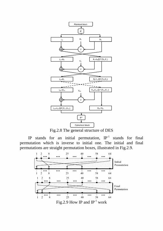
Fig.2.8 The general structure of DES

IP stands for an initial permutation, IP-1 stands for final permutation which is inverse to initial one. The initial and final permutations are straight permutation boxes, illustrated in Fig.2.9.

Fig.2.9 How IP and IP-1 work

IP and IP-1 have no cryptographic significance in DES The block of 64 input bits is divided into two halves: the 32

leftmost bits form L0 and the 32 rightmost bits form R0. DES consists of 16 identical rounds. In each round, new contents of Li and Ri are defined by formula

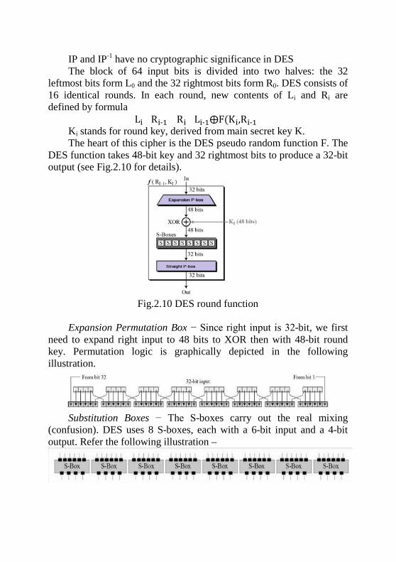
Li=Ri-1 Ri=Li-1⨁F(Ki,Ri-1) Ki stands for round key, derived from main secret key K. The heart of this cipher is the DES pseudo random function F. The

DES function takes 48-bit key and 32 rightmost bits to produce a 32-bit output (see Fig.2.10 for details).

Fig.2.10 DES round function

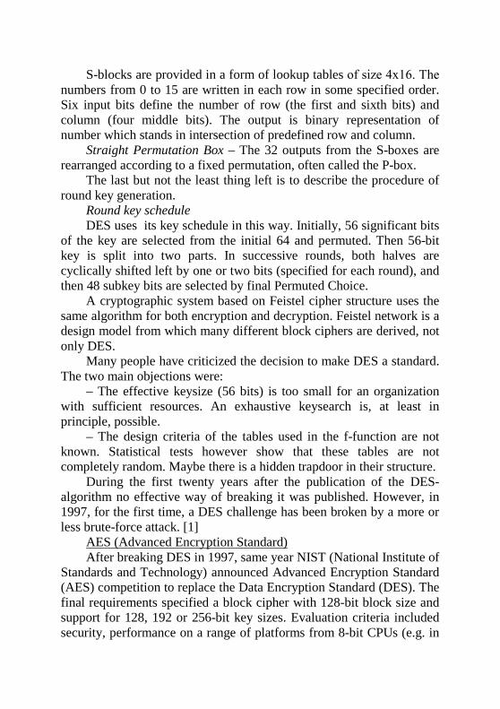
Expansion Permutation Box − Since right input is 32-bit, we first

need to expand right input to 48 bits to XOR then with 48-bit round key. Permutation logic is graphically depicted in the following illustration.

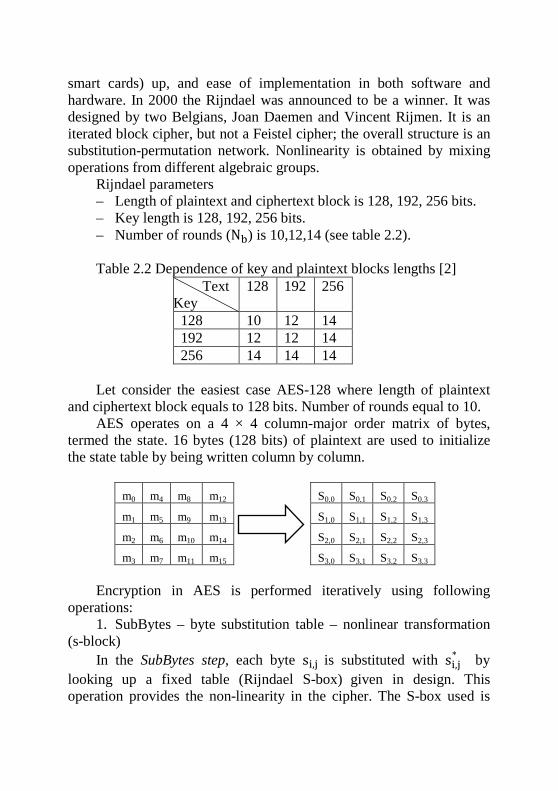
Substitution Boxes − The S-boxes carry out the real mixing

(confusion). DES uses 8 S-boxes, each with a 6-bit input and a 4-bit output. Refer the following illustration –

S-blocks are provided in a form of lookup tables of size 4х16. The numbers from 0 to 15 are written in each row in some specified order. Six input bits define the number of row (the first and sixth bits) and column (four middle bits). The output is binary representation of number which stands in intersection of predefined row and column.

Straight Permutation Box – The 32 outputs from the S-boxes are rearranged according to a fixed permutation, often called the P-box.

The last but not the least thing left is to describe the procedure of round key generation.

Round key schedule DES uses its key schedule in this way. Initially, 56 significant bits

of the key are selected from the initial 64 and permuted. Then 56-bit key is split into two parts. In successive rounds, both halves are cyclically shifted left by one or two bits (specified for each round), and then 48 subkey bits are selected by final Permuted Choice.

A cryptographic system based on Feistel cipher structure uses the same algorithm for both encryption and decryption. Feistel network is a design model from which many different block ciphers are derived, not only DES.

Many people have criticized the decision to make DES a standard. The two main objections were:

– The effective keysize (56 bits) is too small for an organization with sufficient resources. An exhaustive keysearch is, at least in principle, possible.

– The design criteria of the tables used in the f-function are not known. Statistical tests however show that these tables are not completely random. Maybe there is a hidden trapdoor in their structure.

During the first twenty years after the publication of the DES-algorithm no effective way of breaking it was published. However, in 1997, for the first time, a DES challenge has been broken by a more or less brute-force attack. [1]

AES (Advanced Encryption Standard) After breaking DES in 1997, same year NIST (National Institute of

Standards and Technology) announced Advanced Encryption Standard (AES) competition to replace the Data Encryption Standard (DES). The final requirements specified a block cipher with 128-bit block size and support for 128, 192 or 256-bit key sizes. Evaluation criteria included security, performance on a range of platforms from 8-bit CPUs (e.g. in

smart cards) up, and ease of implementation in both software and hardware. In 2000 the Rijndael was announced to be a winner. It was designed by two Belgians, Joan Daemen and Vincent Rijmen. It is an iterated block cipher, but not a Feistel cipher; the overall structure is an substitution-permutation network. Nonlinearity is obtained by mixing operations from different algebraic groups.

Rijndael parameters – Length of plaintext and ciphertext block is 128, 192, 256 bits. – Key length is 128, 192, 256 bits. – Number of rounds (Nb) is 10,12,14 (see table 2.2). Table 2.2 Dependence of key and plaintext blocks lengths [2]

Text Key

128 192 256

128 10 12 14 192 12 12 14 256 14 14 14

Let consider the easiest case AES-128 where length of plaintext

and ciphertext block equals to 128 bits. Number of rounds equal to 10. AES operates on a 4 × 4 column-major order matrix of bytes,

termed the state. 16 bytes (128 bits) of plaintext are used to initialize the state table by being written column by column.

m0 m4 m8 m12 S0,0 S0,1 S0,2 S0,3

m1 m5 m9 m13 S1,0 S1,1 S1,2 S1,3

m2 m6 m10 m14 S2,0 S2,1 S2,2 S2,3

m3 m7 m11 m15 S3,0 S3,1 S3,2 S3,3 Encryption in AES is performed iteratively using following

operations: 1. SubBytes – byte substitution table – nonlinear transformation

(s-block) In the SubBytes step, each byte si,j is substituted with si,j

* by looking up a fixed table (Rijndael S-box) given in design. This operation provides the non-linearity in the cipher. The S-box used is

generated by combining the inverse function (the multiplicative inverse over GF(28)) with an invertible affine transformation. The result is in a matrix of four rows and four columns.

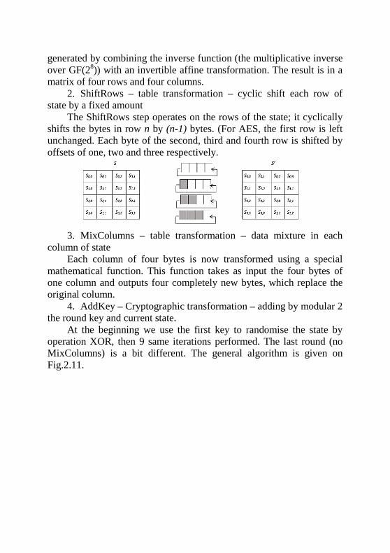
2. ShiftRows – table transformation – cyclic shift each row of state by a fixed amount

The ShiftRows step operates on the rows of the state; it cyclically shifts the bytes in row n by (n-1) bytes. (For AES, the first row is left unchanged. Each byte of the second, third and fourth row is shifted by offsets of one, two and three respectively.

3. MixColumns – table transformation – data mixture in each

column of state Each column of four bytes is now transformed using a special

mathematical function. This function takes as input the four bytes of one column and outputs four completely new bytes, which replace the original column.

4. AddKey – Cryptographic transformation – adding by modular 2 the round key and current state.

At the beginning we use the first key to randomise the state by operation XOR, then 9 same iterations performed. The last round (no MixColumns) is a bit different. The general algorithm is given on Fig.2.11.

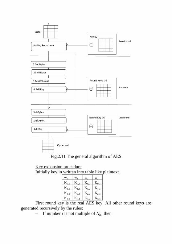
Fig.2.11 The general algorithm of AES

Key expansion procedure Initially key in written into table like plaintext

w0 w1 w2 w3 K0,0 K0,1 K0,2 K0,3 K1,0 K1,1 K1,2 K1,3 K2,0 K2,1 K2,2 K2,3 K3,0 K3,1 K3,2 K3,3

First round key is the real AES key. All other round keys are generated recursively by the rules:

– If number і is not multiple of 𝑁𝑁𝑏𝑏, then

wi = wi-1⨁𝑤𝑤𝑖𝑖−𝑁𝑁𝑏𝑏 – If number і is multiple of 𝑁𝑁𝑏𝑏 (i ⋮ Nb), then

wi = SubBytes(ShiftCol(wi-1)⨁Ri)⨁𝑤𝑤𝑖𝑖−𝑁𝑁𝑏𝑏 The procedure Subbytes means usage of cipher S-block to each

byte of key, operation ShiftCol is a cyclic shift up by one position. 𝑅𝑅𝑖𝑖 is a round constant.

Unlike the Feistel Cipher, the encryption and decryption algorithms needs to be separately implemented, although they are very closely related. All transformations which used for decryption are inverse to correspondent encryption transformation. Each round consists of the four processes conducted in the reverse order with relevant round keys.

– Add round key. – Inv Mix columns – mixture of the byte in column using the

inverse matrix. – Inv Shift rows – cyclic shift bytes to the right. – Inv Byte substitution – substitution operation that used inverse

table SubBytes-1.

2.6 Foundations of Public Key Encryption Symmetric cryptography has few following serious drawbacks:

– the key management problem (too many keys); – the key exchange problem (the necessity of usage the

secure channel prior communication); – the trust problem (authenticity problem).

Public key cryptography was originally invented to solve given problems. The concept of public key cryptography was first presented in the paper of Diffie and Hellman entitled “New Directions in Cryptography” in 1976 [4]. The idea behind public-key cryptosystem is to replace two identical keys for encryption and decryption with two types of keys. Public key is used for encryption and could be published in some directory to be seen by everyone; secret (private) key is used in decryption scheme by its personal owner. Two keys are linked in a mathematical way, such that public key tells nothing about private key. More formally, it could be described in terms of one-way functions which are central to public-key cryptography.

f(x) is called to be one-way function if for given x it is easy to compute f(x), but given f(x) it is hard to compute x. Here, "easy" and "hard" are to be treated in the sense of computational complexity theory, specifically the theory of polynomial time problems.

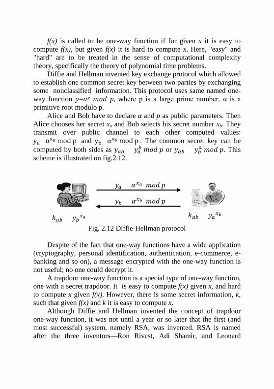
Diffie and Hellman invented key exchange protocol which allowed to establish one common secret key between two parties by exchanging some nonclassified information. This protocol uses same named one-way function 𝑦𝑦=𝛼𝛼𝑥𝑥 𝑚𝑚𝑜𝑜𝑑𝑑 𝑝𝑝, where p is a large prime number, α is a primitive root modulo p.

Alice and Bob have to declare 𝛼𝛼 and p as public parameters. Then Alice chooses her secret xa and Bob selects his secret number xb. They transmit over public channel to each other computed values: ya=αxa mod p and yb=αxb mod p . The common secret key can be computed by both sides as 𝑦𝑦𝑎𝑎𝑏𝑏 = 𝑦𝑦𝑎𝑎

𝑏𝑏 𝑚𝑚𝑜𝑜𝑑𝑑 𝑝𝑝 or 𝑦𝑦𝑎𝑎𝑏𝑏 = 𝑦𝑦𝑏𝑏𝑎𝑎 𝑚𝑚𝑜𝑜𝑑𝑑 𝑝𝑝. This

scheme is illustrated on fig.2.12.

Fig. 2.12 Diffie-Hellman protocol Despite of the fact that one-way functions have a wide application

(cryptography, personal identification, authentication, e-commerce, e-banking and so on), a message encrypted with the one-way function is not useful; no one could decrypt it.

A trapdoor one-way function is a special type of one-way function, one with a secret trapdoor. It is easy to compute f(x) given x, and hard to compute x given f(x). However, there is some secret information, k, such that given f(x) and k it is easy to compute x.

Although Diffie and Hellman invented the concept of trapdoor one-way function, it was not until a year or so later that the first (and most successful) system, namely RSA, was invented. RSA is named after the three inventors—Ron Rivest, Adi Shamir, and Leonard

𝑦𝑦𝑎𝑎 = 𝛼𝛼𝑥𝑥𝑎𝑎 𝑚𝑚𝑜𝑜𝑑𝑑 𝑝𝑝

𝑦𝑦𝑏𝑏 = 𝛼𝛼𝑥𝑥𝑏𝑏 𝑚𝑚𝑜𝑜𝑑𝑑 𝑝𝑝

𝑘𝑘𝑎𝑎𝑏𝑏 = 𝑦𝑦𝑏𝑏𝑥𝑥𝑎𝑎 𝑘𝑘𝑎𝑎𝑏𝑏 = 𝑦𝑦𝑎𝑎

𝑥𝑥𝑏𝑏

Adleman. Security of RSA is based on the difficulty of factoring large numbers.

RSA algorithm can be briefly described by following steps [3]: 1. To generate two large prime numbers p and q. 2. To compute n=p∙q. 3. To select randomly integer e such that greatest common

divisor of e and (p-1)(q-1) equals to 1 (e and (p-1)(q-1) are relatively prime).

4. Using extended Euclidean algorithm to compute the decryption key d such that e∙d≡1 mod (p-1)(q-1). In other words d=e-1 mod (p-1)(q-1).

5. The numbers (n,e) are public key The numbers (p,q,d) are used as secret key. Numbers p and q are not need anymore but should be kept in secret. The simple formula C=Me mod n, M<n can be used for encryption now. To decrypt the message we can use formula M=Cd mod n.

It is obvious that both symmetric and asymmetric methods have a great impact on development of computer networks, internet and other communication means.

2.7 Resilient cryptography In traditional cryptography, primitives are treated as mathematical

objects with a predefined (well-restricted) interface between the primitive and the user/adversary. Based on this view, cryptographers have constructed a plenty of cryptographic primitives (CPA/CCA secure encryption schemes, identification schemes, unforgeable signatures, etc.) from various computational hardness assumption.

Cryptography, however, should be developed for actual deployment in real-world applications and not solely for theoretical purposes. In this new setting, the actual interaction between the primitive and the adversary depends not only on the mathematical description of the primitive, but also on its implementation and the specifics of the physical device on which the primitive is implemented. The information about the primitive leaked to the adversary goes well

beyond that predicted by the designer and, accumulatively, can allow the adversary break an, otherwise secure, primitive. Let consider some attacks based on physical attributes of a computing device which can reveal some information about internal secret key.

Types of Side Channel Attacks Timing Attacks are one of the first type of such attacks which uses

the running time of the execution of a protocol in order to obtain confidential information of user. The adversary knows a set of messages as well as the running time the cryptographic device needs to process them. He can use these running times and potentially (partial) knowledge of the implementation in order to derive information about the secret key. This attack was presented by Paul Kocher in [5], where he describe the results of experiment of timing attack on modular exponentiation and multiplication in RSA on the example of smart cards. The results of the experiment for implementing RSA on a smart card were reported by Schindler and others [6]

OpenSSL is a well-known open source cryptographic library that is often used on Apache web servers to provide SSL functionality. Brumley and Boneh [7] demonstrated that time attacks can reveal RSA private keys from a Web server based on OpenSSL over a local area network.

Power Analysis Attacks: In this kind of attacks, the adversary gets side information by measuring the power consumption of a cryptographic device. Power analysis attack is especially effective in attacks on smart cards or other special embedded systems storing a secret key. In cryptographic implementations where the execution path depends on the processed data, the power trace can reveal the sequence of instructions executed and hence leak information about the secret key. Various examples of power analysis attacks were demonstrated firstly by Kocher in [8]. Power analysis attacks were demonstrated as very powerful attacks for the simplest implementations of a symmetric and asymmetric ciphers in more than 200 papers.

Fault Injection Attacks: These attacks fall into the broader class of tampering attacks. The adversary forces the device to perform erroneous operations (i.e. by flipping some bits in a register). Generally speaking the fault injection attack requires two main steps: the injection of a fault and usage of steps with erroneous operations. If the

implementation is not robust against fault injection, then an erroneous operation might leak information for the secret key. The most common methods of influence are described in [9]. For instance, failures in a smart card can be caused by an impact of environment and placing it in an emergency condition.

Memory Attacks: This type of attack was recently introduced by Halderman in [10]. It is based on the fact that DRAM cells retain their state for long intervals even if the computer is unplugged. Hence an attacker with physical access to the machine can read the content of a fraction of the cells and deduce useful information about the secret key. Halderman et. al. studied the effect of these attacks against DES,AES and RSA. In October 2005, Dag Arne Osvik, Adi Shamir and Eran Tromer presented a paper demonstrating several cache-timing attacks against AES [11].

There are some more less known side channel attacks but leakage-resilient cryptosystems should remain secure even if the attacker learns some arbitrary partial information about their internal secret key through the physical or other leakages. There are some countermeasures can be applied in order to make cryptosystem resilient to side-channel attacks: adding noise, aligning the running time, balancing energy consumption, masking or blinding computing.

Questions to self-checking 1. Classify the cryptographic methods. 2. List types of cryptographic attacks. 3. What a difference between perfect and computational secrecy? 4. Give an example of cipher with perfect secrecy. 5. How to describe LFSR? 6. A5/1 – stream cipher based on LFSR. 7. Data encryption standard (DES). 8. Main operations in AES. 9. Advantages and disadvantages of symmetric cryptography. 10. What Diffie-Hellman protocol can be used for? 11. RSA as one of the best algorithms of asymmetric

cryptosystem. 12. List types of side-channel attacks. 13. Describe the notation of resilient cryptography.

References

1. Henk C.A. van Tilborg, Sushil Jajodia (editors) Encyclopedia of Cryptography and Security. Second edition– Springer, Netherlands 2005. – 1T6841T p.

2. Nigel Smart. Cryptography Made Simple. – Springer, 2016. – 481 p.

3. Gorbenko I.D., Gorbenko Yu.I. Applied Cryptology . Theory. Practice. Application, Kharkiv, Ukraine, Fort Publisher, 2012. – 880 p.

4. Diffie W.; Hellman M. New Directions in Cryptography // IEEE Transactions on Information Theory, Vol. IT-22, No. 6, November 1976. – pp.644-654

5. Paul C. Kocher. Timing attacks on implementations of Diffie-Hellmann, RSA, DSS, and other systems // Advances in Cryptology – CRYPTO '96 :– Springer, 1996. – Vol. 1109. – pp.104–113.

6. 20TW. Schindler. A timing attack against RSA with the Chinese 20TRemainder20T Theorem // Proc. of Cryptographic Hardware and Embedded Systems (CHES 2000), 20TSpringer, 2000, LNCS 1965 20T. – pp.109-124

7. D. Brumley, D. Boneh. Remote Timing Attacks are Practical // Proceedings of the 12th Usenix Security Symposium (August 4–8, 2003), 2003. – pp. 1-13.

8. P. Kocher, J. Jaffe, B. Jun. Differential power analysis. CRYPTO’99,LNCS 1666, 1999. – pp.388-397.

9. Jean-Jacques Quisquater, Francois Koeune (2010-10). Side Channel Attacks. State-of-the-art // CRYPTRECK 2002. – pp. 12-13

10. J. Alex Halderman, Seth D. Schoen, Nadia Heninger, William Clarkson, William Paul, Joseph A. Calandrino, Ariel J. Feldman, Jacob Appelbaum, and Edward W. Felten. Lest We Remember: Cold Boot Attacks on Encryption Keys. In Paul C. van Oorschot, editor,USENIX Security Symposium,2008. – pp. 45–60

11. Dag Arne Osvik; Adi Shamir; Eran Tromer Cache Attacks and Countermeasures: the Case of AES // Proceeding CT-RSA'06

Proceedings of the 2006 The Cryptographers' Track at the RSA conference on Topics in Cryptology. – pp.1-20

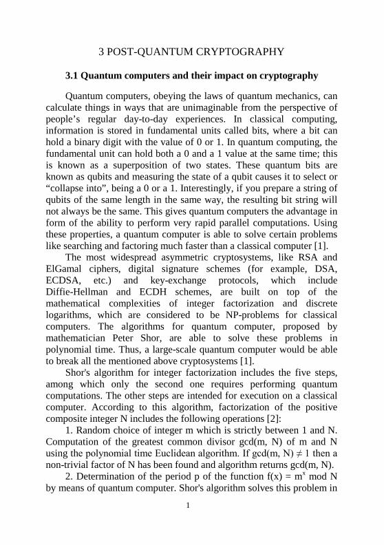
3 POST-QUANTUM CRYPTOGRAPHY 3.1 Quantum computers and their impact on cryptography

Quantum computers, obeying the laws of quantum mechanics, can

calculate things in ways that are unimaginable from the perspective of people’s regular day-to-day experiences. In classical computing, information is stored in fundamental units called bits, where a bit can hold a binary digit with the value of 0 or 1. In quantum computing, the fundamental unit can hold both a 0 and a 1 value at the same time; this is known as a superposition of two states. These quantum bits are known as qubits and measuring the state of a qubit causes it to select or “collapse into”, being a 0 or a 1. Interestingly, if you prepare a string of qubits of the same length in the same way, the resulting bit string will not always be the same. This gives quantum computers the advantage in form of the ability to perform very rapid parallel computations. Using these properties, a quantum computer is able to solve certain problems like searching and factoring much faster than a classical computer [1].

The most widespread asymmetric cryptosystems, like RSA and ElGamal ciphers, digital signature schemes (for example, DSA, ECDSA, etc.) and key-exchange protocols, which include Diffie-Hellman and ECDH schemes, are built on top of the mathematical complexities of integer factorization and discrete logarithms, which are considered to be NP-problems for classical computers. The algorithms for quantum computer, proposed by mathematician Peter Shor, are able to solve these problems in polynomial time. Thus, a large-scale quantum computer would be able to break all the mentioned above cryptosystems [1].

Shor's algorithm for integer factorization includes the five steps, among which only the second one requires performing quantum computations. The other steps are intended for execution on a classical computer. According to this algorithm, factorization of the positive composite integer N includes the following operations [2]:

1. Random choice of integer m which is strictly between 1 and N. Computation of the greatest common divisor gcd(m, N) of m and N using the polynomial time Euclidean algorithm. If gcd(m, N) ≠ 1 then a non-trivial factor of N has been found and algorithm returns gcd(m, N).

2. Determination of the period p of the function f(x) = mx mod N by means of quantum computer. Shor's algorithm solves this problem in

1

polynomial time. 3. If p is odd, the go to the first step. The probability of this is 0.5k

where k is the number of distinct prime factors of N. 4. Since p is even mp - 1 = (m0.5p - 1)(m0.5p + 1) = 0 (mod N). If

m0.5p mod N = -1 then go to the first step. The probability of going backward is less than 0.5k-1, where k denotes the number of distinct prime factors of N.

5. Return of gcd(m0.5p - 1, N) which is computed by the Euclidean algorithm. Since m0.5p mod N = -1, it can be shown that the returned value is a non-trivial factor of N.

Shor's algorithm for discrete logarithm is able to solve the problem of finding the least integer x such that gx mod p = n, where p is a large prime integer, g is a generator of the multiplicative group modulo p and n is positive integer which is less the p. In this case the bivariate function f(a, b) = ga · n-b mod p is being considered. This function has two-dimensional period, which equals (x, 1), because f(a + x, b + 1) = = ga+x · n-b-1 mod p = ga · n-b · gx · n-1 mod p = f(a, b). The considered algorithm uses a quantum computer to find this period in polynomial time and thus determine the value of x [3].

The experts in field of cryptography are starting to catch sight of quantum computing being a matter of near future. A large number of major cryptography specialists in IT industry are of opinion that a fully fledged quantum computer can be constructed in less than 10 years [4]. Moreover, the security of information, which was encrypted by quantum-unsafe cryptosystems, can be achieved only if the time period, during which these data must be kept in secret, is ended before creation of large-scale quantum computer [1]. These circumstances increase the actuality of post-quantum cryptography.

2

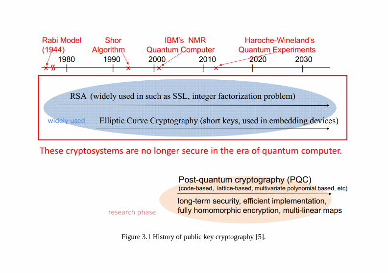
Figure 3.1 History of public key cryptography [5].

3.2 Post-quantum cryptography concept Post-quantum cryptography is a variety of cryptographic

algorithms resistant to attacks using quantum computations. The development of such cryptography requires the investigation of computational problems which cannot be solved in polynomial time by both classical and quantum computers. The main classes of such problems stem from the fields of lattice theory, coding theory and the study of multivariate quadratic polynomials. Each of these classes offers new possible frameworks within which to build public key cryptography. The quantum-safe ciphers that are built on these methods do admittedly present some challenges. Typically, they suffer from large key sizes when compared to popular, current public key algorithms that are not quantum-safe. However, in terms of performance, some quantum-safe algorithms are competitive with – or even faster than – widely used public key algorithms such as RSA or elliptic curve cryptosystems [1].

Some forms of symmetric-key cryptography are guaranteed to be quantum-safe. These primitives make no computational assumptions and are thus information-theoretically secure. An example of this is Vernam’s One Time Pad, which has been proven to have perfect unconditional security against arbitrarily powerful eavesdroppers. Wegman-Carter Authentication is also known to be resistant against quantum attacks [1].

There are also other types of symmetric key cryptography that are believed (but not proven) to be quantum-safe. For example, generic quantum search only provides a quadratic speedup over classical search, indicating that quantum computers could not perform a brute force search to find symmetric keys much faster than could classical computers. Thus, unless the symmetric key algorithm happens to have a particular structure that can be exploited by a quantum computer, the bit security of a symmetric cipher can be retained in the presence of a quantum adversary by simply doubling the key length. Since quantum search does not provide exponential speedups, symmetric key encryption like AES is believed to be quantum-safe. The similar can be stated about good hash functions [1].

Post-quantum asymmetric cryptosystems, which do not use the quantum properties, include the following classes:

1. Code-based cryptosystems where the security depends on the 4

difficulty of solving a decoding problem in a linear code [6]. While there have been some proposals for code-based signatures, code-based cryptography has seen more success with encryption schemes [7]. The classic example is McEliece’s public-key encryption system based on the hidden binary Goppa codes [8].

2. Multivariate cryptosystems where the security depends on the difficulty of solving a system of multivariate polynomial equations over finite fields [6]. While there have been some proposals for multivariate encryption schemes, multivariate cryptography has historically been more successful as an approach to signatures [7]. One of many interesting examples is Patarin’s “HFEv−” public key signature system which generalizes a proposal by Matsumoto and Imai [8].

3. Lattice-based cryptosystems where the security depends on the difficulty of solving a short or close vector problem in a lattice [6]. Most lattice-based key establishment algorithms are relatively simple, efficient, and highly parallelizable [7]. The example that has perhaps attracted the most interest, not the first example historically, is the Hoffstein–Pipher–Silverman “NTRU” asymmetric cryptosystem [8].

4. Hash-based signatures where the security depends on the difficulty of finding collisions or preimages in cryptographic hash functions [6]. Many of the more efficient hash-based signature schemes have the drawback that the signer must keep a record of the exact number of previously signed messages, and any error in this record will result in insecurity. Another of their drawbacks is that they can produce only a limited number of signatures. The number of signatures can be increased, even to the point of being effectively unlimited, but this also increases the signature size [7]. The classic example is Merkle’s hash-tree public-key signature system (1979), building upon a one-message-signature idea of Lamport and Diffie [8].

5. Isogeny-based cryptosystems where the security depends on the difficulty of finding an unknown isogeny between a pair of supersingular elliptic curves. They have good properties such as small key sizes and forward security. These cryptographic schemes are a new research field with relatively few active research groups or publications and deserve more academic scrutiny to establish a consensus on their security properties. The classic example is Jao-De Feo key agreement protocol [6].

5

3.3 Code-based cryptography The main advantage of this class of cryptosystems besides the

quantum resistance is high performance. Its biggest drawback is a large key size which is the reason of less prevalence of these cryptosystems in comparison with RSA and ElGamal schemes [1].

Classical code-based ciphers, like the McEliece and Niederreiter schemes, can be built on top of different linear error-correction codes, but not all of them are suitable to achieve proper security of the obtained cryptosystems. As an example the Niederreiter scheme based on generalized Reed-Solomon codes can be given, which was broken by Sidelnikov and Shestakov with a structural attack. Nevertheless, these cryptosystems based on the hidden binary Goppa codes are secure against attacks by both classical and quantum cryptanalysis [9].

The binary Goppa codes play an important role in ensuring the cryptographic strength of the McEliece and Niederreiter ciphers. Breaking these cryptosystems requires decoding of arbitrary public linear code which was obtained by random transformation of some quickly decodable hidden one. This is an NP-complete problem [9].

There is no known efficient algorithm which allows to distinguish between the binary Goppa code and a binary random one [10]. The number of inequivalent binary Goppa codes grows exponentially with the increase of their length and dimension [11]. These circumstances make impossible to recover in polynomial time a hidden code and reduce the subsequent stage of break of the McEliece and Niederreiter cryptosystems to an effective decoding of the restored code [9].

3.3.1 The McEliece cryptosystem This cryptosystem has been developed by Robert McEliece in

1978 and become the first probabilistic encryption scheme [12]. This cipher uses the mathematical apparatus of matrices and vectors over a field GF(2) and binary linear codes.

The key pair generation includes the following actions [9]: 1. Random choice of a binary linear (n, k)-code С with k × n

generator matrix G. This code must be able to correct no less than t errors and have an efficient decoding algorithm.

2. Random generation of n × n permutation matrix P and nonsingular k × k matrix S.

6

3. Computation of k × n matrix E = S • G • P. 4. Creation of a pair of public and private keys in the form of

tuples (E, t) and (S-1, G, P-1), respectively. The encryption consists of the following steps [9]: 1. Representation of a message as k-dimensional vector m. 2. Calculation of a vector v = m • E. 3. Choice of a random n-dimensional vector z of weight t. 4. Forming of a ciphertext by the formula c = v + z. The decryption requires the following operations [9]: 1. Computation of n-dimensional vector u = c • P-1. 2. Obtainment of vector d as a result of decoding of u with C. 3. Forming of a decrypted message vector m′ = d • S-1. The correctness of this cipher can be proved as follows: 1. A vector u equals c • P-1 = (m • E + z) • P-1 = m • S • G + z • P-1.

Since G is a generator matrix of the linear code C, a vector m • S • G is a word of С. A vector z • P-1 is of weight t, because P is a permutation matrix. Thus, a vector u is a result of distortion of t symbols in a word of С, which was obtained by encoding of a message m • S.

2. A vector d, which is a result of decoding of u with С, has a value m • S as this code allows to correct no less than t errors.

3. A decrypted message vector m′ equals d • S-1 = m. 3.3.2 The Niederreiter cryptosystem This cryptosystem has been proposed by Harald Niederreiter in

1986. Unlike the McEliece cryptographic scheme, it is deterministic, but has a higher speed of encryption and can be used to create a digital signature [13]. However, the generation time for such signatures is more than for other quantum-safe ones [1]. This cipher uses the same mathematical apparatus as the McEliece cryptosystem.

The key pair generation consists of the following steps [9]: 1. Random choice of a binary linear (n, k)-code С with (n – k) × n

parity check matrix H. An efficient decoding algorithm for C must be known. The error correction capability of C should be no less than t.

2. Random generation of n × n permutation matrix P and nonsingular (n – k) × (n – k) matrix S.

3. Calculation of (n – k) × n matrix E = S • H • P. 4. Creation of a pair of public and private keys in the form of

tuples (E, t) and (S-1, H, P-1), respectively. 7

The encryption requires the following operations [3]: 1. Representation of an initial message as n-dimensional vector m

of weight t. 2. Forming of a ciphertext by the formula с = E • mT. The decryption includes the following actions [3]: 1. Computation of (n – k)-dimensional vector u = S-1 • c. 2. Determination of a variable d as a transposed error vector which

corresponds to a syndrome u in the error correction procedure of C. 3. Forming of the decrypted message vector m′ = (P-1 • d)T. The correctness of this cipher can be justified as follows: 1. A vector u equals S-1 • c = S-1 • E • mT = H • P • mT. The weight

of a column vector P • mT equals t, because P is a permutation matrix. Since H is a parity check matrix of the linear code C, u is a syndrome of an error vector (P • mT)T, which has a weight t.

2. A vector d, which is the result of calculation of the transposed error vector which corresponds to a syndrome u in the error correction procedure of the code C, is equal to P • mT, because С is able to correct no less than t errors.

3. A decrypted message vector m′ has a value (P-1 • d)T = m. 3.4 Multivariate cryptography The primary application field of this class of cryptosystems is

digital signature schemes [7]. The main advantages of the multivariate signature schemes are very short signatures and high performance [14]. Their biggest shortcoming is a large key size [8].

To break these cryptosystems one must find a solution of arbitrary public system of multivariate quadratic equations over a finite field. In general, this problem is NP-hard. In multivariate cryptographic schemes the public equation system is obtained by two hidden random linear transformations of some private vector-valued quadratic map, which is easy to invert. Different families within this class of cryptosystems correspond to several approaches to construction of the aforementioned private map [14].

The first multivariate cryptosystem was C* scheme, which has been designed by Matsumoto and Imai in 1985. An approach to break it has been proposed by Patarin in 1995. Other well-known cryptosystems of this class include HFE, UOV, Rainbow and IFS. Some multivariate schemes were broken, but other remain secure both in classical and

8

post-quantum senses [14]. The key pair generation includes the following actions [14]: 1. Random choice of a central map Q which must be an easily

invertible quadratic map between vectors over finite field F. Each n-dimensional vector over F must be mapped by Q to m-dimensional vector over the same finite field. The central map can be represented as m-tuple of n-variate polynomials qi(x1,...,xn) where only quadratic terms are present. The mapping of (v1,...,vn) to (u1,...,um) can be performed according to the formula ui = qi(v1,...,vn).

2. Random choice of initial and final maps S and T, which must be affine maps between vectors over F. The dimensions of mapped vectors are n for S and m for T. The initial map can be represented as n-tuple of linear n-variate polynomials si(x1,...,xn). The mapping of (v1,...,vn) to (u1,...,un), which corresponds to S, can be performed by the formula ui = si(v1,...,vn). The similar holds true for the final map. The mapping formula for T is ui = ti(v1,...,vm) where ti(x1,...,xn) are polynomials of m-tuple representation of the final map.

3. Representation of a map composition P, which equals T ◦ Q ◦ S, as m-tuple of n-variate quadratic polynomials pi(x1,...,xn). The mapping of (v1,...,vn) to (u1,...,um), which corresponds to P, is described by the formula ui = pi(v1,...,vn). The coefficients of the polynomials in the aforementioned m-tuple can be obtained from the identity pi(x1,...,xn) = = ti(q1(s1(x1,...,xn), ..., sn(x1,...,xn)), ..., qm(s1(x1,...,xn), ..., sn(x1,...,xn))).

4. The public key is created in the form of mentioned above polynomial representation of P. The private key must is represented by the tuple (T-1, Q-1, S-1), where the elements correspond to inverse maps.

The message encryption or verification of digital signature can be performed as follows [14]:

1. An initial message or a digital signature is represented as n-dimensional vector d over F.

2. A vector r is obtained as the result of applying of P to d. A ciphertext is represented by r if an encryption is performed. In case of verification a signature is considered invalid if r does not represent the hash of signed message.

The decryption or signing of message consists of the following operations [14]:

1. A ciphertext or a hash of signed message is represented as m-dimensional vector r over F.

9

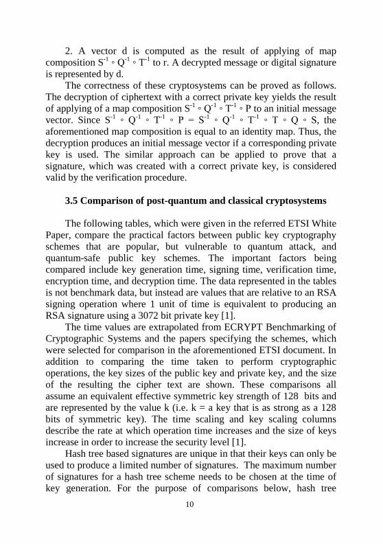
2. A vector d is computed as the result of applying of map composition S-1 ◦ Q-1 ◦ T-1 to r. A decrypted message or digital signature is represented by d.

The correctness of these cryptosystems can be proved as follows. The decryption of ciphertext with a correct private key yields the result of applying of a map composition S-1 ◦ Q-1 ◦ T-1 ◦ P to an initial message vector. Since S-1 ◦ Q-1 ◦ T-1 ◦ P = S-1 ◦ Q-1 ◦ T-1 ◦ T ◦ Q ◦ S, the aforementioned map composition is equal to an identity map. Thus, the decryption produces an initial message vector if a corresponding private key is used. The similar approach can be applied to prove that a signature, which was created with a correct private key, is considered valid by the verification procedure.

3.5 Comparison of post-quantum and classical cryptosystems The following tables, which were given in the referred ETSI White

Paper, compare the practical factors between public key cryptography schemes that are popular, but vulnerable to quantum attack, and quantum-safe public key schemes. The important factors being compared include key generation time, signing time, verification time, encryption time, and decryption time. The data represented in the tables is not benchmark data, but instead are values that are relative to an RSA signing operation where 1 unit of time is equivalent to producing an RSA signature using a 3072 bit private key [1].

The time values are extrapolated from ECRYPT Benchmarking of Cryptographic Systems and the papers specifying the schemes, which were selected for comparison in the aforementioned ETSI document. In addition to comparing the time taken to perform cryptographic operations, the key sizes of the public key and private key, and the size of the resulting the cipher text are shown. These comparisons all assume an equivalent effective symmetric key strength of 128 bits and are represented by the value k (i.e. k = a key that is as strong as a 128 bits of symmetric key). The time scaling and key scaling columns describe the rate at which operation time increases and the size of keys increase in order to increase the security level [1].

Hash tree based signatures are unique in that their keys can only be used to produce a limited number of signatures. The maximum number of signatures for a hash tree scheme needs to be chosen at the time of key generation. For the purpose of comparisons below, hash tree

10

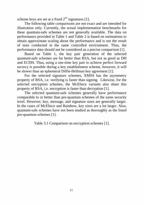
scheme keys are set at a fixed 220 signatures [1]. The following table comparisons are not exact and are intended for

illustration only. Currently, the actual implementation benchmarks for these quantum-safe schemes are not generally available. The data on performance provided in Table 1 and Table 2 is based on estimations to obtain approximate scaling about the performance and is not the result of tests conducted in the same controlled environment. Thus, the performance data should not be considered as a precise comparison [1].

Based on Table 1, the key pair generation of the selected quantum-safe schemes are far better than RSA, but not as good as DH and ECDH. Thus, using a one-time key pair to achieve perfect forward secrecy is possible during a key establishment scheme, however, it will be slower than an ephemeral Diffie-Hellman key agreement [1].

For the selected signature schemes, XMSS has the asymmetry property of RSA, i.e. verifying is faster than signing. Likewise, for the selected encryption schemes, the McEliece variants also share this property of RSA, i.e. encryption is faster than decryption [1].

The selected quantum-safe schemes generally have performance comparable to or better than pre-quantum schemes of the same security level. However, key, message, and signature sizes are generally larger. In the cases of McEliece and Rainbow, key sizes are a lot larger. Also, quantum-safe schemes have not been studied as thoroughly as the listed pre-quantum schemes [1].

Table 3.1 Comparison on encryption schemes [1].

11

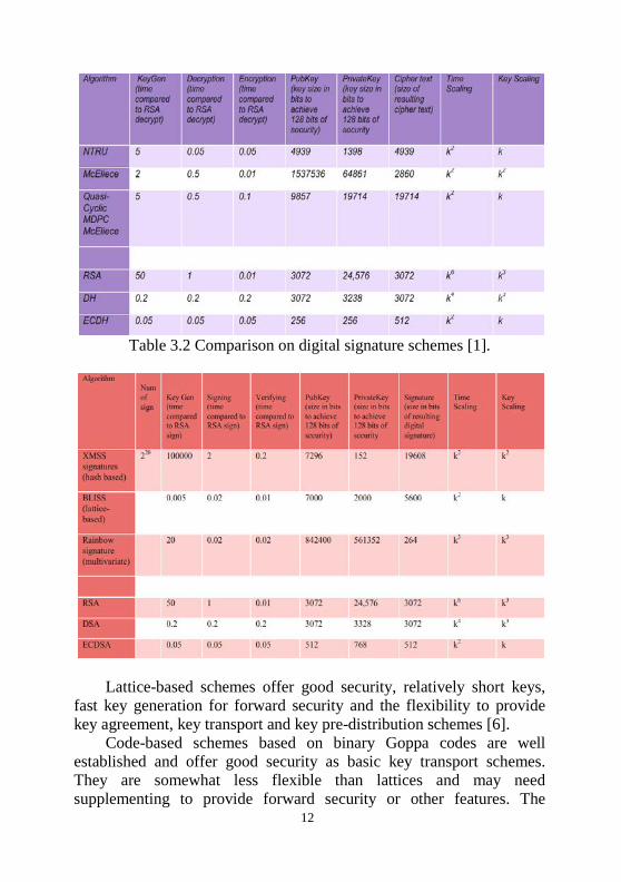
Table 3.2 Comparison on digital signature schemes [1].

Lattice-based schemes offer good security, relatively short keys,

fast key generation for forward security and the flexibility to provide key agreement, key transport and key pre-distribution schemes [6].

Code-based schemes based on binary Goppa codes are well established and offer good security as basic key transport schemes. They are somewhat less flexible than lattices and may need supplementing to provide forward security or other features. The

12

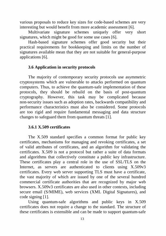
various proposals to reduce key sizes for code-based schemes are very interesting but would benefit from more academic assessment [6].

Multivariate signature schemes uniquely offer very short signatures, which might be good for some use cases [6].

Hash-based signature schemes offer good security but their practical requirements for bookkeeping and limits on the number of signatures available mean that they are not suitable for general-purpose applications [6].

3.6 Application in security protocols The majority of contemporary security protocols use asymmetric

cryptosystems which are vulnerable to attacks performed on quantum computers. Thus, to achieve the quantum-safe implementation of these protocols, they should be rebuild on the basis of post-quantum cryptography. However, this task may be complicated because non-security issues such as adoption rates, backwards compatibility and performance characteristics must also be considered. Some protocols are too rigid and require fundamental messaging and data structure changes to safeguard them from quantum threats [1].

3.6.1 X.509 certificates The X.509 standard specifies a common format for public key

certificates, mechanisms for managing and revoking certificates, a set of valid attributes of certificates, and an algorithm for validating the certificates. X.509 is not a protocol but rather a suite of data formats and algorithms that collectively constitute a public key infrastructure. These certificates play a central role in the use of SSL/TLS on the Internet, as servers are authenticated to clients using X.509v3 certificates. Every web server supporting TLS must have a certificate, the vast majority of which are issued by one of the several hundred commercial certificate authorities that are recognized by major web browsers. X.509v3 certificates are also used in other contexts, including secure email (S/MIME), web services (XML Digital Signatures), and code signing [1].

Using quantum-safe algorithms and public keys in X.509 certificates does not require a change to the standard. The structure of these certificates is extensible and can be made to support quantum-safe

13

algorithms with relative ease. However, X.509 is a standard that is used in many other standards that would require an update to support the newly defined quantum-safe algorithm identifiers. For example, TLS would require new ciphersuites to be introduced [1].

3.6.2 Internet Key Exchange (IKE) version 2 Internet Key Exchange is a protocol used to establish keys and

security associations for the purpose of setting up a secure virtual private network connection that protects network packets from being read or intercepted over a public Internet connection. This allows a remote computer on a public network to access resources and benefit from the security of a private closed network without compromising security [1].

The IKE protocol standard is rigid and does not permit VPN designers to choose beyond a small set of cryptographic algorithms. At present, none of the permitted algorithms are completely quantum-safe. Thus, any option to make IKE quantum-safe would require a change to the standard [1].

3.6.3 Transport Layer Security (TLS) version 1.2 The Transport Layer Security protocol, earlier versions of which

were called the Secure Sockets Layer (SSL) protocol, establishes a protected tunnel between a client and server for transmission of application data. The handshake sub-protocol is used to perform server-to-client and optional client-to-server authentication, and to establish shared secret keys. Shared secrets are subsequently used in the record layer sub-protocol to encrypt and authenticate application data [1].

TLS is used to secure a variety of applications, including web traffic (the HTTP protocol), file transfer (FTP), and mail transport (SMTP). The design of TLS is largely independent of cryptographic algorithms, and allows for parties to negotiate ciphersuites (combinations of cryptographic algorithms to use). As of TLSv1.2, all cryptographic components (public key authentication, key exchange, hash functions, bulk encryption) can be negotiated, although generally all must be negotiated at once in a single ciphersuite rather than independently. Thus, any option to make TLS quantum-safe would

14

require a change to the standards by introducing new ciphersuites. Also, quantum-safe algorithms with large public keys or signatures may require additional changes to the standard to allow certificates with size exciding 16 MB be used [1].

3.6.4 Secure/Multipurpose Internet Mail Extension (S/MIME) Secure/Multipurpose Internet Mail Extension is a standard for

digital signatures and public-key encryption used to securely send email messages. It offers origin authentication, non-repudiation, data integrity, and confidentiality through use of digital signatures and message encryption. This standard is widely adopted throughout government and enterprise. S/MIME, and a similar scheme called OpenPGP, allow email to remain encrypted during the entire path from sender to recipient, meaning that at the email servers of both the sender and receiver, as well as the links between sender, sender's email server, recipient's email server, and receiver, the plaintext cannot be read or modified by an adversary. This contrasts with other protocols like SMTP over TLS and IMAP/POP3 over TLS which are used to secure the individual links between intermediate mail servers, but do not preserve end-to-end confidentiality and data integrity [1].

The S/MIME protocol has the potential to transition to quantum-safe cryptography. The S/MIME Capabilities attribute (which includes algorithms for signatures, content encryption, and key encryption) was designed to be flexible and extensible so that other capabilities added later would not break earlier clients. However, some very early versions of S/MIME may present backward-compatibility issues [1].

3.6.5 Secure Shell (SSH) version 2 Secure Shell version 2 is a cryptographic network protocol used to

encrypt information sent over an insecure network such as the Internet. In essence, it relies on a client-server model to allow a user on one computer to remotely log-in, send commands, and transfer files on another computer, without compromise of data integrity or confidentiality. It has a wide range of uses, with some implementations of SSH (namely OpenSSH) enabling users to create fully encrypted VPNs. This allows users to treat a public network such as the Internet as

15

if it were a more secure, private network [1]. SSH is a secure remote-login protocol. It has pervasive and diverse

applications, and can be used for a variety of purposes, including the construction of cost-effective secure Wide Local Area Networks, secure connectivity for cloud-based services, and essentially any other enterprise process that requires secure remote access to a server [1].

The SSH protocol was specified with a high level of cryptographic agility and allows servers and clients to negotiate the algorithms used for encryption, data integrity, authentication and key exchange. The addition of quantum-safe controls will not require significant changes to the base SSH protocol [1].

3.7 Conclusions The rapid progress in building of quantum computers threatens the

most widespread public key cryptographic schemes. The mathematical problems, which underlie their security, can be solved by quantum algorithms in polynomial time. For example, Shor's algorithms for integer factorization and discrete logarithm allow breaking such cryptosystems as RSA, DSA and Diffie-Hellman schemes. These circumstances increase the actuality of post-quantum cryptography, which is a variety of cryptographic algorithms resistant to attacks using quantum computations.

Symmetric key encryption and good hash functions are believed to be quantum-safe. Asymmetric post-quantum cryptosystems, which use only classical computing, include such classes as code-based, multivariate, lattice-based, hash-based and isogeny-based cryptographic schemes. Their main advantage is high performance, however, these cryptosystems typically suffer from large key sizes.

Multivariate cryptographic schemes are more successfully used to create digital signatures, which in this case are very short. Code-based cryptosystems are primarily applied for encryption. Hash-based cryptography provides an approach only for obtaining digital signatures. Lattice-based cryptosystems have fast generated keys of relatively small size and so are suitable to be used for key agreement. Isogeny-based cryptographic schemes, which are a new research field, possess a significant advantage in the form of very short public key.

16

The majority of security protocols use quantum-unsafe asymmetric cryptosystems and so should be rebuild on the basis of post-quantum cryptography. However, this task may be complicated because non-security issues such as adoption rates, backwards compatibility and performance characteristics must also be considered.

The directions of further research in field of post-quantum cryptography include the investigation of security properties of relatively new quantum-safe cryptographic schemes and search of approaches to obviate the drawbacks of these cryptosystems.

3.8 Questions

1. What are the basic differences between quantum and classical

computers? How does qubit differ from bit? 2. What mathematical problems underlie the most widespread

asymmetric cryptosystems? What quantum algorithms threaten such cryptography?

3. What is a post-quantum cryptography? What advantages and drawbacks do quantum-safe cryptosystems typically have in comparison with widespread public key cryptographic schemes?

4. What are the main classes of post-quantum asymmetric cryptosystems? What mathematical problems underlie their security?

5. What of these cryptography classes are primarily applied for encryption? Which of them are more successfully used for obtaining digital signatures?

6. Why do the binary Goppa codes have an important significance in code-based cryptography?

7. What are the basic differences between the McEliece and Niederreiter schemes? What are the main advantages and drawbacks of these cryptosystems?

8. What is the general approach for construction of equation system of a public key in multivariate cryptography?

9. What is the primary application field of multivariate cryptosystems? What are their main advantages and drawbacks?

10. What issues complicate the introduction of post-quantum cryptography into contemporary security protocols? Which of these protocols possess a low level of cryptographic agility?

11. What is the role of ciphersuites in the cryptographic agility of TLS? How do they impact on the perspective of using the quantum-safe

17

cryptosystems in TLS? 3.9 References

1. M. Campagna, et al., “ETSI White Paper No. 8. Quantum Safe

Cryptography and Security”, European Telecommunications Standards Institute, 2015, 64 p.

2. S. J. Lomonaco, “Shor's Quantum Factoring Algorithm”, AMS Proceedings of Symposia in Applied Mathematics, 2002, vol. 58, 19 p.

3. M. Hayashi, S. Ishizaka, A. Kawachi, G. Kimura, T. Ogawa, “Introduction to Quantum Information Science”, Springer, 2015, 332 p.

4. T. L. Swaim, “Quantum Computing and Cryptography Today: Preparing for a Breakdown”, University of Maryland University College, 2012, 22 p.

5. T. Takagi, “Recent Developments of Post-Quantum Cryptography”, Workshop on Cyber Security between RHUL and Kyushu University, 2016, 22 p.

6. “ETSI GR QSC 001: Quantum-Safe Cryptography (QSC); Quantum-safe algorithmic framework”, European Telecommunications Standards Institute, 2016, 42 p.

7. L. Chen, et al., “NISTIR 8105 DRAFT. Report on Post-Quantum Cryptography”, National Institute of Standards and Technology, 2016, 15 p.

8. D. J. Bernstein, J. Buchmann, E. Dahmen, “Post-Quantum Cryptography”, Springer, 2009, 246 p.

9. E. Jochemsz, “Goppa Codes & the McEliece Cryptosystem”, Vrije Universiteit Amsterdam, 2002, 63 p.

10. T. P. Berger, P.-L. Cayrel, P. Gaborit, A. Otmani, “Reducing Key Length of the McEliece Cryptosystem”, Lecture Notes in Computer Science, 2009, vol. 5580, pp. 77-97.

11. P. Fitzpatrick, J. A. Ryan, “Enumeration of inequivalent irreducible Goppa codes”, Discrete Applied Mathematics, 2006, vol. 154, iss. 2, pp. 399-412.

12. S. Y. Yan, “Quantum Attacks on Public-Key Cryptosystems”, Springer, 2013, 214 p.

13. R. Lu, X. Lin, X. Liang, X. Shen, “An efficient and provably secure public key encryption scheme based on coding theory”, Security and Communication Networks, 2011, vol. 4, iss. 12, pp. 1440-1447.

14. L. Goubin, J. Patarin, B.-Y. Yang, “Multivariate 18

Cryptography”, Encyclopedia of Cryptography and Security, 2011, pp. 824-828.

19

4 SOFTWARE SECURITY AND TECHNOLOGIES FOR RESILIENT COMPUTING

4.1 Understanding software security and resilient software It is difficult enough today to find a business that would not work

on software which objectives and priorities of use differ from organiza-tion to organization and client to client. But in any case you need relia-ble and stable applications. The Institute of Electrical and Electronics Engineers (IEEE) Reliability Society defines reliability as «The target at which software designers have always aimed: perfect operation all the time» [1-2]. However, this does not mean that every element of the system will work reliably all the time, which gives us an understanding of the difference between reliability and resiliency. Resilience in this context means that failures must be compartmentalized [3].

Why is resilient software so important and why not just say “fail-safe” or “failure-resistant”? In a literal sense, “failsafe” means that a system fails in a safe way. On the other hand, the resistive systems re-turn to their original operating state. In most cases, the main way to restore functionality is to restart the entire system: the application, and then, if it did not work, the server, and also have to restart everything that depended on the failed component. On the contrary, a resilient sys-tem automatically shuts down the failover components and reintegrates them as soon as they stop working. So when we talk about software, resilience is the capacity to resist and recover from deliberate attacks, accidents, artificial or natural threats.

Software resilience is the ability of an application to react to trou-bles in one of its components and still provide the best possible service. Resiliency has become more important as business continue to fast im-plement software across multiple technology infrastructures [4-5]. In other words, if application is resilient it means that when faced with any of these changes or even with a combination of them, it must adapt it-self while ensuring the observance of the safety criteria.

In contrast to the challenges of integration of the hardware with software, the abilities of the “hacker” to undermine desired system be-havior also create a significant challenge to application resilience.

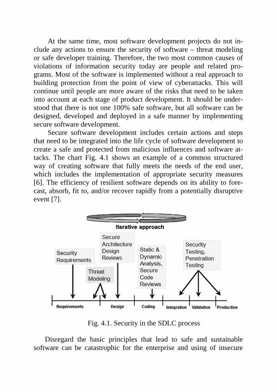
At the same time, most software development projects do not in-clude any actions to ensure the security of software – threat modeling or safe developer training. Therefore, the two most common causes of violations of information security today are people and related pro-grams. Most of the software is implemented without a real approach to building protection from the point of view of cyberattacks. This will continue until people are more aware of the risks that need to be taken into account at each stage of product development. It should be under-stood that there is not one 100% safe software, but all software can be designed, developed and deployed in a safe manner by implementing secure software development.

Secure software development includes certain actions and steps that need to be integrated into the life cycle of software development to create a safe and protected from malicious influences and software at-tacks. The chart Fig. 4.1 shows an example of a common structured way of creating software that fully meets the needs of the end user, which includes the implementation of appropriate security measures [6]. The efficiency of resilient software depends on its ability to fore-cast, absorb, fit to, and/or recover rapidly from a potentially disruptive event [7].

Fig. 4.1. Security in the SDLC process

Disregard the basic principles that lead to safe and sustainable software can be catastrophic for the enterprise and using of insecure

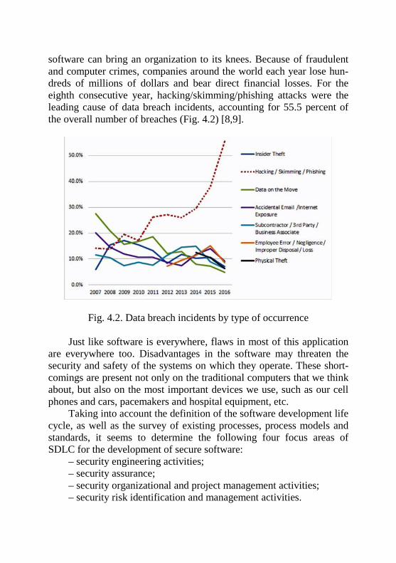
software can bring an organization to its knees. Because of fraudulent and computer crimes, companies around the world each year lose hun-dreds of millions of dollars and bear direct financial losses. For the eighth consecutive year, hacking/skimming/phishing attacks were the leading cause of data breach incidents, accounting for 55.5 percent of the overall number of breaches (Fig. 4.2) [8,9].

Fig. 4.2. Data breach incidents by type of occurrence

Just like software is everywhere, flaws in most of this application are everywhere too. Disadvantages in the software may threaten the security and safety of the systems on which they operate. These short-comings are present not only on the traditional computers that we think about, but also on the most important devices we use, such as our cell phones and cars, pacemakers and hospital equipment, etc.

Taking into account the definition of the software development life cycle, as well as the survey of existing processes, process models and standards, it seems to determine the following four focus areas of SDLC for the development of secure software:

– security engineering activities; – security assurance; – security organizational and project management activities; – security risk identification and management activities.

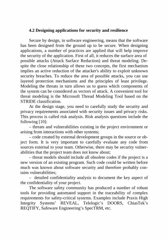
4.2 Designing applications for security and resilience Secure by design, in software engineering, means that the software

has been designed from the ground up to be secure. When designing applications, a number of practices are applied that will help improve the security of the application. First of all, it reduces the surface area of possible attacks (Attack Surface Reduction) and threat modeling. De-spite the close relationship of these two concepts, the first mechanism implies an active reduction of the attacker's ability to exploit unknown security breaches. To reduce the area of possible attacks, you can use layered protection mechanisms and the principles of least privilege. Modeling the threats in turn allows us to guess which components of the system can be considered as vectors of attack. A convenient tool for threat modeling is the Microsoft Thread Modeling Tool based on the STRIDE classification.

At the design stage, you need to carefully study the security and privacy requirements associated with security issues and privacy risks. This process is called risk analysis. Risk analysis questions include the following [10]:

– threats and vulnerabilities existing in the project environment or arising from interactions with other systems;

– code created by external development groups in the source or ob-ject form. It is very important to carefully evaluate any code from sources external to your team. Otherwise, there may be security vulner-abilities that the project team does not know about;

– threat models should include all obsolete codes if the project is a new version of an existing program. Such code could be written before much was known about software security and therefore probably con-tains vulnerabilities;

– detailed confidentiality analysis to document the key aspect of the confidentiality of your project.

The software safety community has produced a number of robust tools for providing automated support in the traceability of complex requirements for safety-critical systems. Examples include Praxis High Integrity Systems’ REVEAL, Telelogic’s DOORS, ChiasTek’s REQTIFY, Safeware Engineering’s SpecTRM, etc.

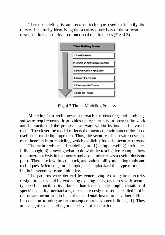
Threat modeling is an iterative technique used to identify the threats. It starts by identifying the security objectives of the software as described in the security non-functional requirements (Fig. 4.3).

Fig. 4.3 Threat Modeling Process Modeling is a well-known approach for detecting and studying-

software requirements. It provides the opportunity to present the work and interaction of the proposed software within its intended environ-ment. The closer the model reflects the intended environment, the more useful the modeling approach. Thus, the security of software develop-ment benefits from modeling, which explicitly includes security threats.

The main problems of modeling are: 1) doing it well; 2) do it care-fully enough; 3) knowing what to do with the results, for example, how to convert analysis in the metric and / or in other cases a useful decision point. There are few threat, attack, and vulnerability modeling tools and techniques. Microsoft, for example, has emphasized this type of model-ing in its secure software initiative.

The patterns were derived by generalizing existing best security design practices and by extending existing design patterns with securi-ty-specific functionality. Rather than focus on the implementation of specific security mechanisms, the secure design patterns detailed in this report are meant to eliminate the accidental insertion of vulnerabilities into code or to mitigate the consequences of vulnerabilities [11]. They are categorized according to their level of abstraction:

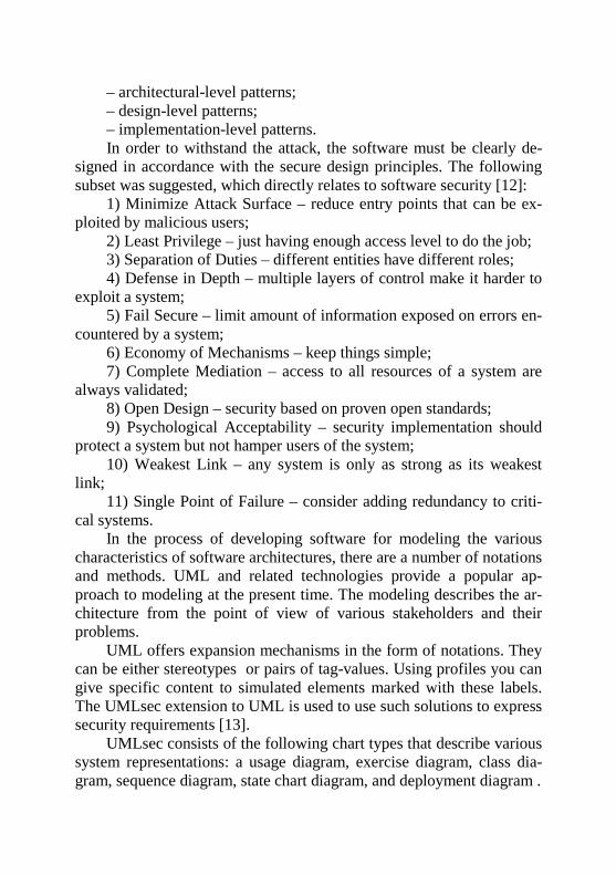
– architectural-level patterns; – design-level patterns; – implementation-level patterns. In order to withstand the attack, the software must be clearly de-

signed in accordance with the secure design principles. The following subset was suggested, which directly relates to software security [12]:

1) Minimize Attack Surface – reduce entry points that can be ex-ploited by malicious users;

2) Least Privilege – just having enough access level to do the job; 3) Separation of Duties – different entities have different roles; 4) Defense in Depth – multiple layers of control make it harder to

exploit a system; 5) Fail Secure – limit amount of information exposed on errors en-

countered by a system; 6) Economy of Mechanisms – keep things simple; 7) Complete Mediation – access to all resources of a system are

always validated; 8) Open Design – security based on proven open standards; 9) Psychological Acceptability – security implementation should

protect a system but not hamper users of the system; 10) Weakest Link – any system is only as strong as its weakest

link; 11) Single Point of Failure – consider adding redundancy to criti-

cal systems. In the process of developing software for modeling the various

characteristics of software architectures, there are a number of notations and methods. UML and related technologies provide a popular ap-proach to modeling at the present time. The modeling describes the ar-chitecture from the point of view of various stakeholders and their problems.

UML offers expansion mechanisms in the form of notations. They can be either stereotypes or pairs of tag-values. Using profiles you can give specific content to simulated elements marked with these labels. The UMLsec extension to UML is used to use such solutions to express security requirements [13].

UMLsec consists of the following chart types that describe various system representations: a usage diagram, exercise diagram, class dia-gram, sequence diagram, state chart diagram, and deployment diagram .

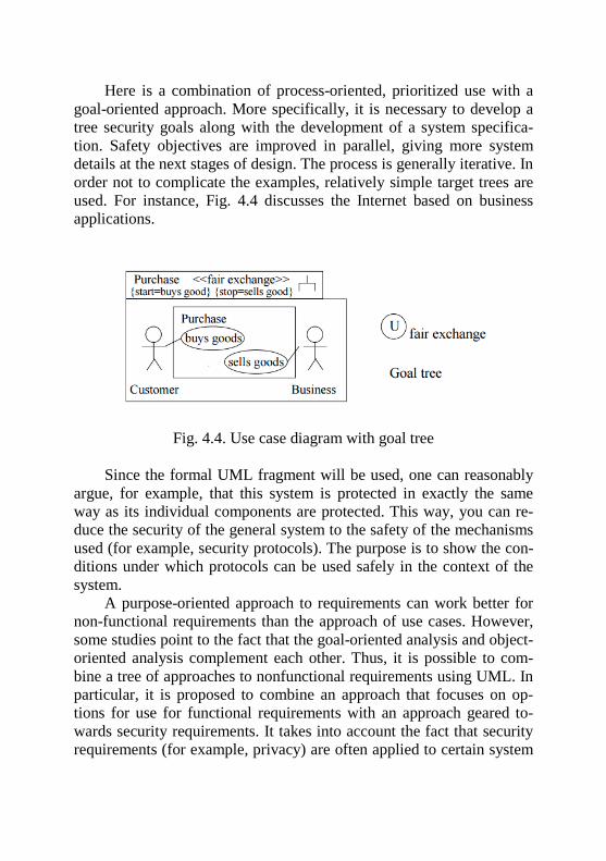
Here is a combination of process-oriented, prioritized use with a goal-oriented approach. More specifically, it is necessary to develop a tree security goals along with the development of a system specifica-tion. Safety objectives are improved in parallel, giving more system details at the next stages of design. The process is generally iterative. In order not to complicate the examples, relatively simple target trees are used. For instance, Fig. 4.4 discusses the Internet based on business applications.

Fig. 4.4. Use case diagram with goal tree Since the formal UML fragment will be used, one can reasonably

argue, for example, that this system is protected in exactly the same way as its individual components are protected. This way, you can re-duce the security of the general system to the safety of the mechanisms used (for example, security protocols). The purpose is to show the con-ditions under which protocols can be used safely in the context of the system.

A purpose-oriented approach to requirements can work better for non-functional requirements than the approach of use cases. However, some studies point to the fact that the goal-oriented analysis and object-oriented analysis complement each other. Thus, it is possible to com-bine a tree of approaches to nonfunctional requirements using UML. In particular, it is proposed to combine an approach that focuses on op-tions for use for functional requirements with an approach geared to-wards security requirements. It takes into account the fact that security requirements (for example, privacy) are often applied to certain system

functions, and not to the system as a whole, since application of the security requirement for the whole system may be impracticable.

4.3 Secure Coding. Testing for Security Depending on the software development process or design ap-

proach used, as well as the design and development, coding and testing schedules, it can be performed several times, can be performed at dif-ferent times for different parts of the software, or can be performed simultaneously with the actions of other phases. At the stage of soft-ware coding, the following security issues should be considered:

– selecting the programing language; – selecting the compiler, library, and runtime; – agreements and coding rules; – comments; – documentation of security-sensitive codes, designs and imple-

mentation solutions; – integration of non-development software; – required for filters and wrappers. Practically in all software methods testing is integrated into the

coding phase with minimal debugging and modular testing. A lot of information on specific methods of writing secure code

are published. Some of them are organized in a language or platform. Many of them are aimed at a mass audience and do not assume any knowledge about the creation of software. Those principles that are cit-ed by most studies and that are in fact secure coding and secure archi-tecture / design are presented, for example, in [14].

The secure coding standards offered by the CERT CMU are based on documented versions in the standard language. To date, CERT has published secure encoding standards for C (ISO / IEC 9899: 1999 / Cor 3: 2007) and C ++ (ISO / IEC 9899: 1999 / Cor 3: 2007), with plans to publish additional standards for the Sun Microsystems API for Java2 platform Standard Edition 5.0 Specification and programming language Microsoft C # (ISO / IEC 23270: 2006).

Security analysis and software testing is performed regardless of the kinds of software functionality. Its function is to evaluate the securi-ty properties of this software when interacting with external objects, such as users, the user environment, other software, and interacting

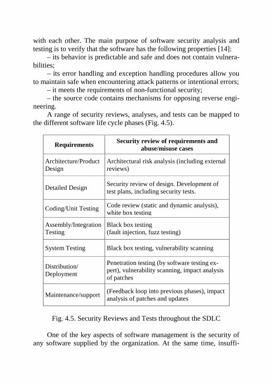
with each other. The main purpose of software security analysis and testing is to verify that the software has the following properties [14]:

– its behavior is predictable and safe and does not contain vulnera-bilities;

– its error handling and exception handling procedures allow you to maintain safe when encountering attack patterns or intentional errors;

– it meets the requirements of non-functional security; – the source code contains mechanisms for opposing reverse engi-

neering. A range of security reviews, analyses, and tests can be mapped to

the different software life cycle phases (Fig. 4.5).

Requirements Security review of requirements and abuse/misuse cases

Architecture/Product Design

Architectural risk analysis (including external reviews)

Detailed Design Security review of design. Development of test plans, including security tests.

Coding/Unit Testing Code review (static and dynamic analysis), white box testing

Assembly/Integration Testing

Black box testing (fault injection, fuzz testing)

System Testing Black box testing, vulnerability scanning

Distribution/ Deployment

Penetration testing (by software testing ex-pert), vulnerability scanning, impact analysis of patches

Maintenance/support (Feedback loop into previous phases), impact analysis of patches and updates

Fig. 4.5. Security Reviews and Tests throughout the SDLC

One of the key aspects of software management is the security of

any software supplied by the organization. At the same time, insuffi-

cient attention is paid to testing program security and fixing vulnerabili-ties at earlier stages of the development lifecycle, without waiting for testing for vulnerabilities of the finished application. Security code au-dit is a structural testing of software to identify vulnerabilities, the im-plementation of which can reduce the level of integrity, availability and confidentiality of the system. An important feature of security code se-curity technologies is that the main task of the audit is to identify not all possible vulnerabilities, but only code vulnerabilities that can be ex-ploited by an attacker.

In general terms, code security auditing is an iterative process, in-cluding planning, analysis, recommendations for finalizing the program and documentation, and developing methods and tools for identifying and analyzing vulnerabilities [15].

We list the main classes of these vulnerabilities: – overflow, read and write outside the buffer; – the output of calculations beyond a certain range when convert-

ing variables of a numerical type; – the formation of a negative value for the length of a string of

bytes or the number of elements in the array; – incorrect casting; – lack of initialization of data; – leak, shortage, use of freed memory; – time and synchronization errors; – errors of locks in multithreaded environments, etc. These vulnerability classes can be used to perform denial of ser-

vice attacks or execute illegitimate code. There are several methods for auditing code security: – viewing (inspecting) the code manually; – static code analysis by template; – dynamic analysis of code execution. The first approach is considered the most effective in terms of

completeness and accuracy of the checks. The shortcomings of the method include high labor intensity and requirements for qualifications and experience of experts. Static code analysis using a template consists in the use of automation tools for searching and analyzing potentially dangerous code constructs (signatures) in the source code of programs. This method is effective when searching for simple vulnerabilities and non-maskable bookmarks, such as buffer overflow, password constants

or "logical bombs". The automated methods for carrying out the static method by template include vulnerability scanners for PREfix, PREfast, AK-Sun, UCA, FlawFinder, ITS4, RATS, FxCop.

Modern code scanners allow to some extent automate: – search for buffer overflow vulnerabilities; – search for OS-injections (execution of arbitrary commands); – SQL injection search; – search for XSS queries (crossite scripting); – search for errors in input and output values; – carrying out a structural analysis of subprograms that implement

protection functions. Numerous studies have shown that the cost of fixing vulnerability

after the end of development can be several hundred times higher than the cost of solving the problem in an application that is still being de-veloped.

A penetration test (or pentest) is a practical way to show how much software is protected from threats to information security [16]. There is also the term ethical hacking.

This method simulates a set of "hacker" attacks, the purpose of which is to penetrate the company's internal network infrastructure, steal and / or modify confidential data, and disrupt critical business processes.

Unlike real intruders, the team of testers observes certain ethical rules in carrying out all works: any dangerous actions are committed only by prior agreement with the customer; the entire scanning process is transparent and planned.

Conducting testing for the penetration of software systems requires professionals, in-depth knowledge of IT security, the ability to think outside the box, apply social engineering techniques, collect and ana-lyze information, as well as creativity.

There are both open and commercial methodologies for conduct-ing penetration tests that are capable of ensuring a guaranteed quality of the service when the whole process is observed. However, in practice the use of only one methodology is not advisable, as a rule, they are used modularly with the necessary revision.

The most popular methodologists of ethical hacking: – Information Systems Security Assessment Framework (OISSG); – The Open Source Security Methodology Manual (OSSTMM);

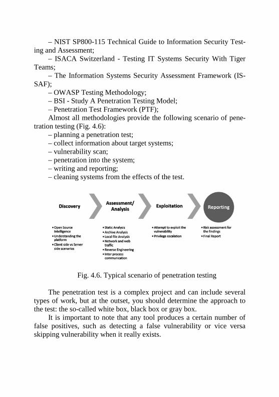
– NIST SP800-115 Technical Guide to Information Security Test-ing and Assessment;

– ISACA Switzerland - Testing IT Systems Security With Tiger Teams;

– The Information Systems Security Assessment Framework (IS-SAF);

– OWASP Testing Methodology; – BSI - Study A Penetration Testing Model; – Penetration Test Framework (PTF); Almost all methodologies provide the following scenario of pene-

tration testing (Fig. 4.6): – planning a penetration test; – collect information about target systems; – vulnerability scan; – penetration into the system; – writing and reporting; – cleaning systems from the effects of the test.

Fig. 4.6. Typical scenario of penetration testing The penetration test is a complex project and can include several

types of work, but at the outset, you should determine the approach to the test: the so-called white box, black box or gray box.

It is important to note that any tool produces a certain number of false positives, such as detecting a false vulnerability or vice versa skipping vulnerability when it really exists.

Since new vulnerabilities in software and technologies are detected almost daily, the penetration test is a complex and voluminous service that can show the current picture of the security of software products.

4.4 Implementing security and resilience into software When the development of secure software is intended, the overall

structure of the technological process is preserved, but at each step ad-ditional security measures are taken. Thus, the process of developing secure software is a set of measures that are aimed at providing the re-quired level of information security developed by the software product. There are many methods for developing secure software. The method-ologies that consider the construction of secure software involve re-sources that address particular phases or focus on specific platforms. Most of them are introduced by the largest software developers and various government organizations. The choice of methodology depends entirely on the desired result.

The development of secure software is still closely related to rec-ommendations, best practices and undocumented expertise. The ap-proaches of modern practices provide guidance for specific areas, such as threat modeling, risk management or secure coding. It is important that they be integrated into a comprehensive development method. De-spite some improvements in the definition of processes for the devel-opment of secure software, these processes are conditioned by the expe-rience of experts. Therefore, it is difficult for developers to evaluate them, assess their strengths and resist their weaknesses. An objective comparison of these methodologies is still an urgent task, and it is diffi-cult for various stakeholders to make a measured decision about which one is more suitable for work.

Next, consider several "ready-to-use" SDLC-methodologies with appropriate information resources that are designed specifically to cre-ate secure software. A basic of characteristics will be discussed in order to describe their overall meaning.

Comprehensive, Lightweight Application Security Process (CLASP) [17]. CLASP is the process of creating secure software and contains a set of 24 activities and additional resources that need to be adapted to the development process in use.

Features of the methodology:

– the main goal of CLASP is to support the creation of software primarily from a security perspective;

– CLASP is defined as a set of independent actions that must be integrated into the development process and its working environment. However, this is not an integrated process. The frequency of implemen-tation of activities is indicated on individual activities, which leads to complex coordination. Two road maps give some recommendations on how to combine actions into a single and ordered set;

– CLASP defines roles and assigns actions to these roles. Roles can influence the security situation and are used as an additional per-spective for structuring a set of actions;

– CLASP provides a set of security resources, one of which is a list of 104 known types of problems. They determine the basis of secu-rity vulnerabilities in the source code of the application.

Security Development Lifecycle (SDL) [18]. SDL was created by Microsoft to solve security problems and in-

cludes a set of activities that complement the development process of Microsoft and is designed as an addition to the process of creating software.

Features of the methodology: – SDL's main goal is to improve the quality of software-oriented

software. Most often, this activity is related to the development on the basis of functionality. Because the architecture can primarily reduce security threats, threat modeling begins with architectural dependencies with external systems. However, little attention is paid to the imple-mentation and integration of security mechanisms in the methodology;

– the SDL process is well organized, and related activities are grouped in stages. Specific security stages are comparable with the standard stages of software development, and some activities are con-tinuous in the SDL process (for example, threat modeling and educa-tion). Support for revising and improving intermediate results is also present in the SDL process;

– SDL well describes the methods for performing actions, which on average are specific and pragmatic. In particular, the use of flowcharts reduces the attack surface, and threat modeling is described as a more detailed process. Thus, performing some operations is possi-ble even for less experienced developers.

TSP-Secure [19, 20].

CMU’s SEI and CERT Coordination Center (CERT/CC) devel-oped the Team Software Process for Secure Software Development (TSP-Secure). The purpose of creating TSP-Secure was to reduce or eliminate software vulnerabilities that arise from design and software errors. An important problem is also the ability to predict the likelihood of vulnerability in the software. In doing so, TSP provides a systematic way for software developers and managers to learn how to implement methods in an organization.

TSP-Secure implements security practices throughout the SDLC and provides approaches and methods for:

– establishment of operational procedures, organizational policies, management oversight, resource allocation, training, planning and pro-ject tracking;

– analysis of vulnerabilities by type of defects; – establishment of safety-related forecasting indicators, control

points and safety-related measurements; – risk management and feedback; – secure design, use of design patterns to avoid common vulnera-

bilities and develop security reviews; – quality management for secure programming, the use of secure

language subsets and coding standards, static and dynamic analysis tools;

– security checks, which include the development of plans for var-ious types of security testing;

– remove vulnerabilities from the software. Secure Software Engineering (S2e) [21]. SSDM is a unified model that combines some of the existing secu-

rity technologies with the software development process. The process of creating secure software is divided into five stages: – security training. The essence of security training is to provide

training in security matters; – threat modeling. Since common security criteria may not be suit-

able for all software products, each software development must have its own threat model;

– security specification (SS). This implies directing directions and procedures that guarantee the security of the software;

– SS review. Assumes checking the compliance of software design content;

– penetration testing. The capabilities of the software to prevent at-tacks are tested.

Secure Tropos [22]. Tropos2 is a software development methodology focused on the

agent, designed to describe the organizational environment of the multi-agent system and the system itself. Three key aspects:

– consider all stages of system development, adopting a uniform and homogeneous method based on the concept of agents: subjects, goals, objectives, resources and intentional dependencies;

– Tropos pays great attention to early requirements, and also how the proposed system will meet its organizational goals;

– the methodology is based on the idea of constructing a model of the system, which is gradually refined and expanded from the concep-tual level to the executed artifacts. This allows developers to accurately check the development process, detailing the higher-level representa-tions presented in the previous development stages.

Using the Tropos2 methodology to address security and resilience issues at all stages of software development, the following three objec-tives should be considered:

– determine the requirements for system security; – develop a project that meets the specified safety requirements; – to approve the developed system in respect of safety. Thus, Secure Tropos provides a well-managed process that pro-

vides developers with security concerns through various modeling ac-tivities. The use of the same concepts and designations at all stages of development acts as a key point in the methodology of Secure Tropos.

Undoubtedly, there are more research results on the development of secure software than it was presented above, for example, [10, 14].

Conclusions Now that you have completed this webquest on Computer Security

you are now aware of the possible security treats to computer systems. Not only that, but you are now better able to protect your computers as well as recommend security measures to others.

Questions for self-control 1. When designing a software architecture, which quality attribute

do you value more: flexibility or resilience? 2. What is difference between functional and non-functional re-

quirements in software designing? 3. What is software resilience? 4. What are the Software Development Life Cycle (SDLC) phases? 5. Why is it important to create a threat model for each software

product separately? 6. Describe the main features Secure Software. 7. According to SSDM what are the phases of creating secure soft-

ware? 8. What is the main goal of CLASP? 9. What is the purpose of creating TSP-Secure? 10. Explain why does security is a non-functional requirements. 11. What tool is using due to security requirements and test case

generation? 12. What can the result of buffer overflows exploitation? 13. What are UMLSec notation diagrams? 14. What is secure design pattern? References 1. Avizienis. A., Laprie. J.-C.. Randell, B.. Landwehr. C.: Basic

concepts and taxonomy of dependable and secure computing. IEEE Trans, on Dependable and Secure Computing 1. 11-33 (2004).

2. The Difference Between Reliable and Resilient Software. Ac-cessed at: http://cabforward.com/the-difference-between-reliable-and-resilient-software/.

3. Trivedi, K.S., Kim. D.S.. Ghosh. R.: Resilience in computer sys-tems and networks. In: Proc. of Int. Conf. on Computer-Aided Design - ICCAD 2009. p. 74. ACM Press, New York (2009).

4. Laprie. J.-C.: From dependability to resilience. In: 38th Annual IEEE/IFIP International Conference on Dependable Systems and Net-works. Fast Abstracts (2008).

5. Gorbenko, A., Kharchenko, V., Mamutov, S., Tarasyuk. O., Romanovsky, A.: Exploring Uncertainty of Delays as a Factor in End-

to-End Cloud Response Time. In: 2012 Ninth European Dependable Computing Conference, pp. 185-190. IEEE (2012).

6. Security in the SDLC process. Accessed at: https://www. owasp.org/index.php?title=File:S-SDLC_TP.jpg&setlang=en.

7. Merkow, Mark S. Secure and resilient software development / Mark S. Merkow, Lakshmikanth Raghavan.

8. Data Breaches Increase 40 Percent in 2016, Finds New Report from Identity Theft Resource Center and CyberScout. Accessed at: http://www.idtheftcenter.org/2016databreaches.html.

9. Model-based evaluation of the resilience of critical infrastruc-tures under cyber attacks

10. Karen Mercedes Goertzel, Allen Hamilton. Enhancing the De-velopment Life Cycle to Produce Secure Software. Accessed at: https://www.researchgate.net/publication/228704603_Enhancing_the_Development_Life_Cycle_to_Produce_Secure_Software.

11. Chad Dougherty, Kirk Sayre, Robert C. Seacord, David Svo-boda, Kazuya Togashi. Secure Design Patterns. Accessed at: https://resources.sei.cmu.edu/library/asset-view.cfm?assetid=9115.

12. Samuel T. Redwine, Jr., ed., Secure Software: a Guide to the Common Body of Knowledge to Produce, Acquire, and Sustain Secure Software. Available from: https://buildsecurityin.us-cert.gov/daisy/bsi/resources/dhs/95.html?branch=1&language=1.

13. Jan JürjensSiv Hilde Houmb. Risk-Driven Development of Se-curity-Critical Systems Using UMLsec. Accessed at: https://link.springer.com/chapter/10.1007/1-4020-8159-6_2.

14. Software Security Assurance State-of-the-Art Report (SOAR). Accessed at: https://www.csiac.org/wp-content/uploads/ 2016/02/security.pdf.

15. Security Code Review in the SDLC. Accessed at: https://www.owasp.org/index.php/Security_Code_Review_in_the_SDLC.

16. Ric Messier. Penetration Testing Basics: A Quick-Start Guide to Breaking into Systems / Apress, 2016. – 115 p.

17. Open Web Application Security Project (OWASP) CLASP Project Webpage. Accessed at: https://www.owasp.org/index.php/ CLASP_Concepts.

18. Lipner, Steve and Michael Howard. “The Trustworthy Compu-ting Security Development Lifecycle”. Microsoft Developer Network,

March 2005. Accessed at: https://msdn.microsoft.com/uk-ua/enus/library/ms995349.aspx.

19. Over, James W. “TSP for Secure Systems Development” (presentation). Accessed at: https://www.sei.cmu.edu/tsp/tsp-securepresentation/tsp-secure.pdf.

20. Schneider, Thorsten. “Secure Software Engineering Processes: Improving the Software Development Life Cycle to Combat Vulnera-bility”. Software Quality Professional. Volume 8 Issue 1, December 2006. Available from: https://secure.asq.org/perl/msg.pl?prvurl= http://asq.org/pub/sqp/past/vol9_issue1/sqpv9i1schneider.pdf.

21. A. S. Sodiya, S. A. Onashoga, and O. B. Ajayi. Towards Building Secure Software Sysems. Accessed at: https://www.researchgate.net/publication/249724183_Towards_Building_Secure_Software_Systems.

22. Mouratidis, Haralambos and Paolo Giorgini (2007) “Secure Tropos: A Security-Oriented Extension of the Tropos Methodology”. International Journal of Software Engineering and Knowledge Engi-neering, Volume 17 No. 2, April 2007, pages 285-309. Accessed 25 August 2008 at: http://www.dit.unitn.it/~pgiorgio/papers/IJSEKE06-1.pdf

АННОТАЦИЯ

В разделе актуализирована проблема информационной без-опасности программных продуктов и освещено понятие резиль-ентного программного обеспечения.

Раздел содержит описания практик безопасного проектирова-ния приложений и нотации UMLsec, которые используются для создания защищенных программных систем.

В разделе рассмотрено типовые уязвимости программного обеспечения, техники безопасного кодирования, приёмы динами-ческого и статического анализа кода, обосновано важность прове-дения тестирования на проникновение.

Также раздел содержит описание ключевых особенностей наиболее популярных методологий создания безопасного про-граммного обеспечения.

У розділі актуалізовано проблему інформаційної безпеки про-грамних продуктів та висвітлено поняття резільєнтного програм-ного забезпечення.

Розділ містить опис практик безпечного проектування про-грам і нотацій UMLsec, які використовуються для створення за-хищених програмних систем.

У розділі розглянуто типові вразливості програмного забезпе-чення, техніки безпечного кодування, прийоми динамічного і ста-тичного аналізу коду, обґрунтовано важливість проведення тесту-вання на проникнення.

Також розділ містить опис ключових особливостей найбільш популярних методологій створення безпечного програмного за-безпечення.

In the section the problem of information security of software products is actualized and the concept of resilient software is covered.

The section contains descriptions of security application design practices and UMLsec notations that are used to create secure software systems.

The section describes typical software vulnerabilities, secure encoding techniques, dynamic and static code analysis techniques, the importance of conducting penetration testing is justified.

The section also describes the key features of the most popular methodologies for secure software development.

1

PART 2. FUNDAMENTALS OF FORMAL METHODS FOR

SYSTEM SECURITY

GLOSSARY ...................................................................................... 4

CHAPTER 5. Introduction to formal methods .................................. 4

5.1 What are Formal Methods? ......................................................... 8

5.2 The Nature of Formal Methods ................................................. 10

5.3 Benefits in the use of Formal Methods ...................................... 16

5.4 Limitations to the use of Formal Methods ................................. 18

CHAPTER 6 Formal Analysis and Design for Security Engineering and

resilience .......................................................................................... 26

6.1 Knowledge Acquisition for automated Specifications – Goal-

Oriented Requirements of the Security Engineering ....................... 27

6.2 Formal Analysis and Design for Security Engineering ............. 38

6.3 A Formal Framework for Dependability and Resilience from a

Software Engineering Perspective ................................................. 102

Definition of a formal conceptual framework for dependability and

resilience ........................................................................................ 105

Entities, Properties and satisfiability ............................................. 106

Subjectivity of satisfaction using observers and balancing ........... 110

Change, Evolution Axis and Correlations ..................................... 114

Nominal Satisfiability and Requirements ...................................... 117

The Nominal Mode ........................................................................ 145

Entities, Observers, Properties and Balancing ............................... 149

Evolution and Observation axis ..................................................... 151

2

The Satisfiability view ................................................................... 152

Tolerance, failure and Resilience .................................................. 157

Other Approaches for DREF Satisfiability functions .................... 157

Conclusion ..................................................................................... 159

7 Formal Methods for Architecting Secure Software Systems...... 172

Introduction ................................................................................... 173

7.1 Semi-formal Security Modelling and Analysis Approaches ... 175

7.2 MAC-UML Framework .......................................................... 176

7.3 SecureUML ............................................................................. 178

7.4 Separating Modelling of Application and Security Concerns . 180

7.5 Formal Security Modelling and Analysis Approaches ............ 182

7.6 Integrated Semi-formal and Formal Modelling and Analysis

Approaches .................................................................................... 188

7.7 Aspect-Oriented Security Modelling and Analysis Approaches191

7.8 Discussion ................................................................................ 195

8 Formal Methods for Assuring Security of Protocols .................. 197

8.1 Security primer ........................................................................ 203

8.2 Needham–schroeder protocol .................................................. 206

8.3 Belief logics ............................................................................. 208

8.4 Process algebras ....................................................................... 211

8.5 Associating keys and principals .............................................. 220

8.6 Conclusions ............................................................................. 223

9. Formal Methods for the Analysis of Security Protocols ........... 227

9.1 The Abadi-Rogaway Soundness Theorem .............................. 228

9.2 Soundness in the Presence of Key-Cycles ............................... 235

9.3 Partial Leakage of Information ................................................ 246

3

9.4 Information-Theoretic Interpretations: Soundness and

Completeness for One-Time Pad ................................................... 253

9.5 A General Treatment for Symmetric Encryption .................... 256

4

GLOSSARY

API – Application Programming Interface

AS – Autonomous system

DES - Data Encryption Standard

DSA - Digital Signature Algorithm

DFS - depth first search

ICTS - Information and Communication Technological systems

BPMN - Business Process Model and Notation

DREF -Dependability and Resilience Engineering Framework

DSL - domain specific modelling languages

SPL - software product line

CSP - Communicating sequential processes

RF - REACT framework

CCS - Calculus of Communicating Systems

CC - Common Criteria

EAL - Evaluation Assessment Level

CICS - Customer Information Control System

OOA - object-oriented analysis

VDM - Vienna Development Method

OSSD - Open Source Software Development

SUMO - Upper Merged Ontology

TAF - Test Automation Framework

SCR - Software Cost Reduction

XML - Extensible Markup Language

DoS - denial of service

CICS - Customer Information Control System

GUI - Graphical user interface

UCM - Use Case Maps

GRL - GALS Representation Language

UCM - Use Case Maps

FDAF - Formal Design Analysis Framework

5

GSE - Genetic Software Engineering

R2D2C - Requirements to Design to Code

HR - Human Resources

STC - short term contracts

OCL - Object Constraint Language

QCO - Quality Control Officer

DNS - Domain Name System

KAOS - Knowledge Acquisition for autOmated Specifications

UML - Unified Modeling Language

AADL - Architecture Analysis and Design Language

CERT/CC - Computer Emergency Readiness Team Coordination

Center

OCL - Object Constraint Language

PKI - public-key infrastructure

MAC - Mandatory Access Control

SSL - secure sockets layer

RBAC - role-based access control model

MCA - multiple certification-authority

KDM - key-dependent message

OTP - One-Time Pad

EJB - Enterprise JavaBeans

SMASC - Separating Modelling of Application and Security

Concerns

SAM - Software Architecture Model

COI - Conflict of interest classes

Multilevel Security (MLS)

DARPA -Defense Advanced Research Projects Agency

PCA - Polymorphous Computing Architecture

AAP - Avionics Application Process

EPE - Encryption Processing Element

NSE - Network Security Element

DAC - Discretionary Access Control

DTLTS - discrete-time transition labeled transition system

6

CVS - Concurrent Versions System

AOSD - Oriented Software Development

PIM - Personal Information Management

ED - Embedded Device

FADSE - Formal Analysis and Design for Security Engineering

ID – Identifier

IEEE – Institute of Electrical and Electronics Engineers

IP – Internet Protocol

JFK - Just Fast Keying

GA - General Attacker

LAN – Local Area Network

MAS - multi-agent systems

7

CHAPTER 5. INTRODUCTION TO FORMAL METHODS

Content of the CHAPTER 5

5.1 What are Formal Methods?Ошибка! Закладка не определена.

5.2 The Nature of Formal MethodsОшибка! Закладка не определена.

5.3 Benefits in the use of Formal MethodsОшибка! Закладка не определена.

5.4 Limitations to the use of Formal MethodsОшибка! Закладка не определена.

8

5.1 What are Formal Methods?

The term “formal methods” has come into common use (and abuse)

during the past years. In this book we take a fairly liberal interpretation

of the term. We include, for example, not only “mainstream” formal

methods such as Event-B, Z, VDM, CSP and CCS, but also other

programming and system design paradigms which are underpinned by

discrete mathematics, for example code generation and transformation,

techniques and tools for static analysis of programs, and programming

languages with sound semantics [1-7].

A software specification and production method, based on a

mathematical system, that comprises: a collection of mathematical

notations addressing the specification, design and development phases

of software production; a well-founded logical system in which formal

verification and proofs of other properties can be formulated; and

methodological framework within which software may be verified from

the specification in a formally verifiable manner.

This is a rather ambitious definition. Formal methods are attractive,

but in practice most them in common use do not address the full

spectrum of design, some supporting specification phases, some the

construction phases, and others the analysis of systems.

Typically, formal methods have three components:

- a notion of “program”;

- a means of expressing properties of the computation of

programs;

- some method for establishing whether a program has some

property.

Each of these is rigorously mathematically defined. This is a fairly

liberal description of a formal method. It covers things like the type

inference system of some modern programming languages which

“prove” programs have a well-formed type, to entirely general purpose

theorem proving systems or proof assistants, or paper and pencil

methods. The quality of evidence one gets from a formal method varies

according to the method but generally it is highly accurate, is

convincing to trained workers, and often has a rather narrow coverage

because it abstracts from many detailed features of systems.

9

There is also a wide range of formality and rigour applied in the use

of formal methods. A formal proof might consist of justifying a

conjecture by deriving it from the basic axioms of the mathematics

upon which the logical system in use is based. A rigorous argument

looks more like an outline of how a proof might proceed, but would not

supply all the intervening detail. Additionally, rigorous argument may

draw upon a rich body of known results, but without the need for

formally integrating them into a proof. Note that this is how engineers

and mathematicians usually work—they customarily have a commonly

understood context which obviates the need to descend into detail

which obscures the main subject. However computer based proof tools

do not have the insight of mathematicians, and cannot interpolate

unstated detail between steps. Computer based proofs are therefore

usually very detailed, and can be extremely obscure, although their

validity is potentially less contentious than a rigorous argument [8-16]. The mathematical basis of formal methods may be an existing part

of mathematics—for example the Z specification language has set

theory at its heart—or can be developed anew for the method—the

Calculus of Communicating Systems has a theory presented in an

algebraic style, but specific to the Calculus. There is a large and growing variety of formal methods, of varying

age and maturity. It must be realised that there is no “standard” formal

method. Each technique has particular strengths and weaknesses and it

may be that in the course of systems development it is appropriate to

use a number of methods at different stages of the process. Just as in

traditional engineering, no single theory encompasses all aspects of

design and development. Many theoretical approaches are used—either

explicitly or implicitly. “Stock answers” are often brought to bear and,

even if these appear not to involve mathematics directly, they usually

have a long history of mathematical analysis which has consolidated

into a precise understanding of the nature and behaviour of a particular

aspect of the component or structure. The interaction and compositional

properties of such components are well understood and the properties

of the whole (strength, weight, current, speed, loading, cost, time to

construct, etc.) can all be predicted with much more accuracy than is

now possible with comparable computer systems development.

10

The need for and impact of this use of theory is also well

understood by managers, engineers’ licensors and procurers.

Comparable use of methods or theories is currently not so diverse in the

area of computer systems engineering and it is desirable that engineers

cultivate a broad awareness of possible methods which are relevant to

different aspect of systems design and develop the ability to assess the

usefulness and applicability for particular applications of competing or

complementary approaches. Just as there is no standard formal method, there is (as yet) no

standard way of applying any particular formal method. As case study

material and tools are developed to support the engineering domain,

this may change. However until then it is likely that engineering

application of formal methods will require to be open in nature with the

partial success or failure of certain approaches expected and the results

of this failure used to inform more successful application. As with other engineering disciplines, a body of “good practice”

should provide guidance to engineers as to effective use of techniques

within different contexts. Unfortunately with formal methods this

material is sparse, of variable quality, and not well indexed. In due

course this body of information will grow, in particular it is hoped that

a range of texts and real-world case studies will be produced. Let us go on to present the capabilities and limitations of formal

methods, and guidance for their uptake.

5.2 The Nature of Formal Methods

Software and systems engineering have a number of different life

cycle models, however most break down into a number of phases of

activity such as: requirements, specification, design, implementation

and test [17-23].

A common view of the use of formal methods in this regime might

expect the following. The customer interacts with the supplier closely

over requirements. The supplier writes a formal specification, which is

then successively refined as implementation detail is added until an

implementation results. This is then subjected to test. The use of formal

methods at the various stages of refinement can mean that the final

implementation in some sense is proven to satisfy the top-level

specification. The ‘proof of satisfaction’ is one of the documents which

11

may be required by the certification authority as part of any licensing

procedure.

Traditionally this kind of approach has been seen as the goal of

formal methods research and there is still considerable academic

investigation into approaches which aim to achieve this. However the

level of “correctness” delivered must be interpreted within a broad

engineering framework—the meaning of the word to the customer may

be very different to that assumed by the designer. Absolute correctness

is unattainable—it is not a concept that is familiar to (or sought by)

engineers in other disciplines, they do however make extensive use of

mathematics to model, design and analyse.

In this hierarchy the requirement and specification layer generally

say mostly what the system is required to do. The lower layers (and

there is usually more than just one step at each level) contain increasing

amounts of implementation detail how the system is to achieve its

function. Correspondingly the amount of information at each level

increases as we descend, usually very rapidly.

Let us comment on and elaborate this model. There are several

observations to be made. Note that many of these are not necessarily

restricted to formal methods, but are often true of software engineering

in general.

Requirements are never right

The symptom of the supplier delivering what he was asked for and

the customer only then realising that the original requirements were

wrong or ambiguous is common. This is one of the major problems in

systems and software engineering. Close interaction between the

customer and the supplier is desirable at all stages of development, but

identifying problems as early as possible in the life-cycle is highly

desirable. Use of formal methods at the requirements stage can increase

the clarity of understanding and so reduce the scope for

misinterpretation with the corresponding saving of wasted development

effort, saving both time and money.

One approach is to use a formal method that supports executable

specifications. This does indeed allow experimentation with statements

of requirements and can result in a significant “feel good” factor for the

customer as they have something concrete (i.e. runable) in their hands

early on. However, this can mean that implementation level decisions

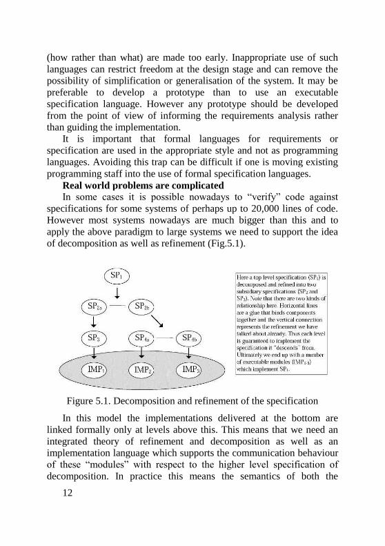
12

(how rather than what) are made too early. Inappropriate use of such

languages can restrict freedom at the design stage and can remove the

possibility of simplification or generalisation of the system. It may be

preferable to develop a prototype than to use an executable

specification language. However any prototype should be developed

from the point of view of informing the requirements analysis rather

than guiding the implementation.

It is important that formal languages for requirements or

specification are used in the appropriate style and not as programming

languages. Avoiding this trap can be difficult if one is moving existing

programming staff into the use of formal specification languages.

Real world problems are complicated

In some cases it is possible nowadays to “verify” code against

specifications for some systems of perhaps up to 20,000 lines of code.

However most systems nowadays are much bigger than this and to

apply the above paradigm to large systems we need to support the idea

of decomposition as well as refinement (Fig.5.1).

Figure 5.1. Decomposition and refinement of the specification

In this model the implementations delivered at the bottom are

linked formally only at levels above this. This means that we need an

integrated theory of refinement and decomposition as well as an

implementation language which supports the communication behaviour

of these “modules” with respect to the higher level specification of

decomposition. In practice this means the semantics of both the

13

specification language and the implementation language must be

related formally so that the behaviour of the implementation is

adequately proven to satisfy the higher level specification.

An alternative approach is to use a single “wide spectrum”

language. These are languages which support both specification and

implementation activities. The term “wide spectrum” is used to refer to

the spectrum of activities in system development. In some cases they

provide mechanisms for verifying the code against specification, or

support formal refinement of code from specifications. Although these

exist in prototype form this area is still the subject of much research.

One benefit of the approach in figure 5.1 is the separation of

concerns possible under this model. It may be possible to isolate critical

aspects of system behaviour in a small number of components. The use

of formal methods to ensure integrity of these components can then be

more focused. Traditional techniques may then be adequate for the

remainder, although great care must be taken over interfaces.

Formality is internal to the model above

Even if the formal proof of correctness of implementation against

specification exists this still only represents a part of the final system.

The implementation will be expressed in some high level programming

language. This will require to be compiled to object code, probably

with the linking in of library components. This then runs on some

hardware. It is possible to verify components such as compilers, library

function and hardware, but these would generally use different

techniques and to reason about the “correctness” of the composition of

all of these is a considerable task requiring significant intellectual and

economic investment. These kinds of activities usually require strategic

sponsorship, and involvement of academic groups, although we can

expect results of this work to become viable (technically and

economically) in the industrial context during the next decade [24-28].

Other problems arise in that the resulting system has to interface

with the environment which includes unpredictable entities like people

or analogue components often in an asynchronous environment. Here

the main problem is one of validation of the system with respect to its

environment. Here again formal methods can help. One can model

interfaces, and use these to explore the operating conditions of the

plant, thus exposing the requirements on the operator, as well as the

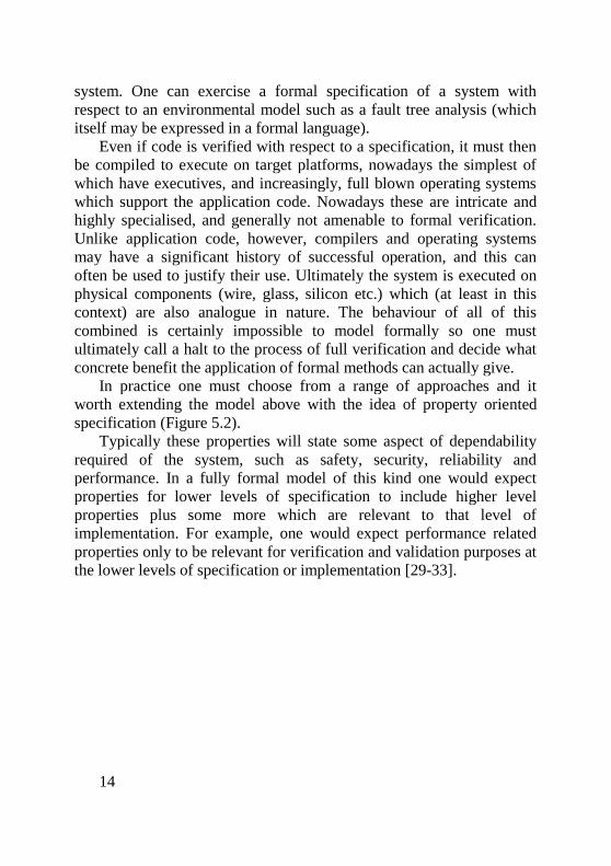
14

system. One can exercise a formal specification of a system with

respect to an environmental model such as a fault tree analysis (which

itself may be expressed in a formal language).

Even if code is verified with respect to a specification, it must then

be compiled to execute on target platforms, nowadays the simplest of

which have executives, and increasingly, full blown operating systems

which support the application code. Nowadays these are intricate and

highly specialised, and generally not amenable to formal verification.

Unlike application code, however, compilers and operating systems

may have a significant history of successful operation, and this can

often be used to justify their use. Ultimately the system is executed on

physical components (wire, glass, silicon etc.) which (at least in this

context) are also analogue in nature. The behaviour of all of this

combined is certainly impossible to model formally so one must

ultimately call a halt to the process of full verification and decide what

concrete benefit the application of formal methods can actually give.

In practice one must choose from a range of approaches and it

worth extending the model above with the idea of property oriented

specification (Figure 5.2).

Typically these properties will state some aspect of dependability

required of the system, such as safety, security, reliability and

performance. In a fully formal model of this kind one would expect

properties for lower levels of specification to include higher level

properties plus some more which are relevant to that level of

implementation. For example, one would expect performance related

properties only to be relevant for verification and validation purposes at

the lower levels of specification or implementation [29-33].

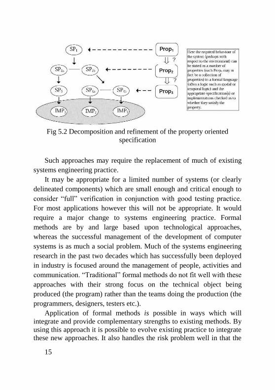
15

Fig 5.2 Decomposition and refinement of the property oriented

specification

Such approaches may require the replacement of much of existing

systems engineering practice.

It may be appropriate for a limited number of systems (or clearly

delineated components) which are small enough and critical enough to

consider “full” verification in conjunction with good testing practice.

For most applications however this will not be appropriate. It would

require a major change to systems engineering practice. Formal

methods are by and large based upon technological approaches,

whereas the successful management of the development of computer

systems is as much a social problem. Much of the systems engineering

research in the past two decades which has successfully been deployed

in industry is focused around the management of people, activities and

communication. “Traditional” formal methods do not fit well with these

approaches with their strong focus on the technical object being

produced (the program) rather than the teams doing the production (the

programmers, designers, testers etc.).

Application of formal methods is possible in ways which will

integrate and provide complementary strengths to existing methods. By

using this approach it is possible to evolve existing practice to integrate

these new approaches. It also handles the risk problem well in that the

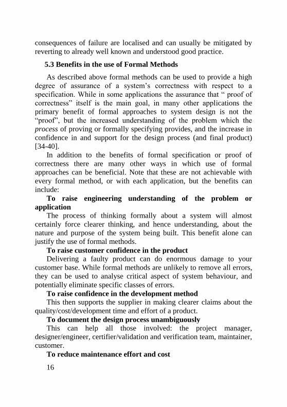
16

consequences of failure are localised and can usually be mitigated by

reverting to already well known and understood good practice.

5.3 Benefits in the use of Formal Methods

As described above formal methods can be used to provide a high

degree of assurance of a system’s correctness with respect to a

specification. While in some applications the assurance that “ proof of

correctness” itself is the main goal, in many other applications the

primary benefit of formal approaches to system design is not the

“proof”, but the increased understanding of the problem which the

process of proving or formally specifying provides, and the increase in

confidence in and support for the design process (and final product)

[34-40].

In addition to the benefits of formal specification or proof of

correctness there are many other ways in which use of formal

approaches can be beneficial. Note that these are not achievable with

every formal method, or with each application, but the benefits can

include:

To raise engineering understanding of the problem or

application

The process of thinking formally about a system will almost

certainly force clearer thinking, and hence understanding, about the

nature and purpose of the system being built. This benefit alone can

justify the use of formal methods.

To raise customer confidence in the product

Delivering a faulty product can do enormous damage to your

customer base. While formal methods are unlikely to remove all errors,

they can be used to analyse critical aspect of system behaviour, and

potentially eliminate specific classes of errors.

To raise confidence in the development method

This then supports the supplier in making clearer claims about the

quality/cost/development time and effort of a product.

To document the design process unambiguously

This can help all those involved: the project manager,

designer/engineer, certifier/validation and verification team, maintainer,

customer.

To reduce maintenance effort and cost

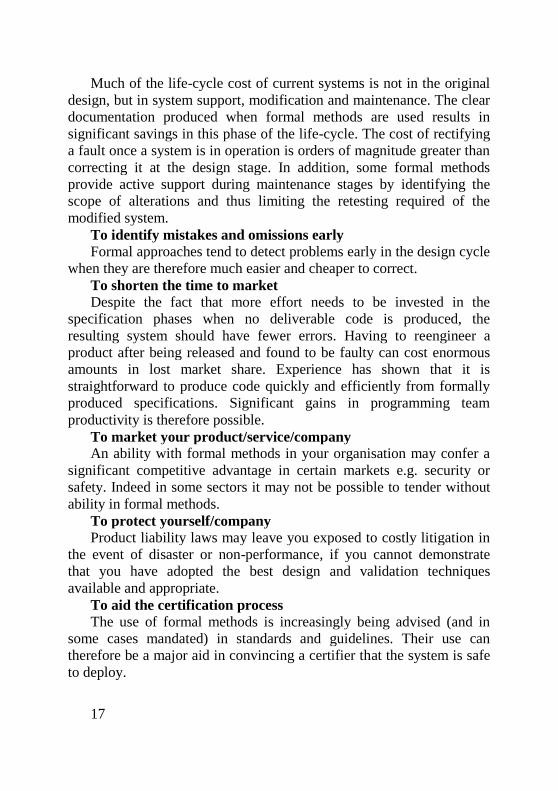
17

Much of the life-cycle cost of current systems is not in the original

design, but in system support, modification and maintenance. The clear

documentation produced when formal methods are used results in

significant savings in this phase of the life-cycle. The cost of rectifying

a fault once a system is in operation is orders of magnitude greater than

correcting it at the design stage. In addition, some formal methods

provide active support during maintenance stages by identifying the

scope of alterations and thus limiting the retesting required of the

modified system.

To identify mistakes and omissions early

Formal approaches tend to detect problems early in the design cycle

when they are therefore much easier and cheaper to correct.

To shorten the time to market

Despite the fact that more effort needs to be invested in the

specification phases when no deliverable code is produced, the

resulting system should have fewer errors. Having to reengineer a

product after being released and found to be faulty can cost enormous

amounts in lost market share. Experience has shown that it is

straightforward to produce code quickly and efficiently from formally

produced specifications. Significant gains in programming team

productivity is therefore possible.

To market your product/service/company

An ability with formal methods in your organisation may confer a

significant competitive advantage in certain markets e.g. security or

safety. Indeed in some sectors it may not be possible to tender without

ability in formal methods.

To protect yourself/company

Product liability laws may leave you exposed to costly litigation in

the event of disaster or non-performance, if you cannot demonstrate

that you have adopted the best design and validation techniques

available and appropriate.

To aid the certification process

The use of formal methods is increasingly being advised (and in

some cases mandated) in standards and guidelines. Their use can

therefore be a major aid in convincing a certifier that the system is safe

to deploy.

18

5.4 Limitations to the use of Formal Methods

It is important to realise limitations in the use of formal methods, as

well as their benefits. Outlined below are some of the disadvantages or

potential problems which may arise and should be taken into account in

making a decision on whether to use formal methods.

Formal methods can be expensive to do

Perhaps more accurately—formal methods will be expensive the

first time you try them.

It is important to amortise start-up costs across a spread of projects

and time and to start out with simple and easily achievable aims,

ramping up as technical experience grows. This said, the use of

experienced consultants in the early stages on use of formal methods

will usually be a low risk and cost effective route to adoption.

There is no formulaic approach

Case study material is sparse. This will improve in time and with

experience, but you must expect to view projects from an applied

research perspective rather than established engineering practice.

Appropriate risk management techniques must be used. The use of

appropriately experienced consultants for early ventures in the field can

reduce both cost and risk.

Training time

This varies by method, but it takes at least several months for even

a well motivated engineer to become familiar with the use of formal

methods in design. (Attaining a reading capability can be much quicker

though).

Difficulties of communications

Using formal methods to communicate can increase accuracy, but

does require a change in attitude, and some training. This can be a

particular problem with customers and management who do not have

the technical incentive to become familiar with them. Integrating

formal methods into existing development methods, and proper use of

interspersed text and engineering diagrams and notations, can mitigate

the problem.

The complexity/size problem

Although formal methods are improving their range of application

the problem of scaling up to larger examples can be problematic.

Abstraction is a common approach in many engineering disciplines for

19

handling such complexity. In systems engineering however our

understanding of approaches to abstraction is not well developed.

Again the use of skilled consultants or staff can help here.

Formal methods are weak on performance

Research is improving in this area, for example in the development

of timed calculi, and in integrating with more traditional performance

approaches, but it will be some time before these mature.

Poor formal infrastructure

While principles of applications of formal methods are well

understood, maximum benefit requires adequate formal infrastructure.

For example almost all programming languages do not have a usable

formal semantics. This makes the behavioural analysis of code difficult,

even though formal methods might have been used earlier in the

development cycle. Similarly no usable verified compilers exist, so

how can one be sure of the “correctness” of object code.

Cultural uncertainty surrounding formal methods

Formal methods are a moving target. Which ones work in what

domain? What is next year’s method going to be? Will I have to

completely retrain?

The validation problem

Formal methods apply to abstractions. Real systems are too

complicated to analyse fully. (This is true in traditional engineering as

well though). Can I validate my model with respect to the expected

behaviour of the whole system? What level of

requirement/specification is appropriate?

Lack of tools

Although the situation is improving tool coverage is still poor, and

doing formal methods by hand is time consuming, error prone and

usually will require a higher level of expertise. It’s a bit like trying to

write a program without a compiler. Even simple tools such as syntax

and type checking tools can strongly support the use of formal methods.

Formal methods do not substitute for creative thinking

In fact even more is required to bring together traditional design

capability with the new approach. It is important that existing expertise

and practice are properly utilised with the introduction of formal

methods.

Advancement questions

20

1. What components do formal methods have?

2. What does a formal proof mean?

3. What are the formal methods designed for?

4. What is a rigorous argument in context of the formal methods?

5. What are the main problems in the construction of the formal

methods?

6. What are the formal language used for?

7. What is the main idea of the decomposition and refinement of the specification?

8. What is the main feature of the property oriented

specification?

9. What are the main benefits in the use of formal methods?

10. What are the main limitations to the use of Formal Methods

REFERENCES

1. Anderson S. O. Guidance on the use of Formal Methods in the

Development and Assurance of High Integrity Industrial

Computer Systems / S. O. Anderson, R. E. Bloomfield, G. L.

Cleland // European workshop on industrial computer systems

technical committee 7 (Safety, Reliability and Security). –

1998. – pp.34.

2. Popov P. Application of Formal Methods (Poster Session)-

Reliability Assessment of Legacy Safety-Critical Systems

Upgraded with Off-the-Shelf Components / P. Popov // Lecture

Notes in Computer Science. – 2002. – № 2434. – p. 139-150.

3. Vain J. Refinement-based development of timed systems / J.

Vain, J. Berthing, P. Boström, K. Sere, L. Tsiopoulos //

International Conference on Integrated Formal Methods. –

2012. – №1. – p. 69-83.

4. Vain J. Model Checking–A New Challenge for Design of

Complex Computer-Controlled Systems / J. Vain, R. Kyttner //

Proc. of 5-th International Conference on Engineering Design

and Automation. – 2001. – №2. – p. 593-598.

21

5. Vain J. Model checking of emergent behaviour properties of

robot swarms / J. Vain, S. Juurik //

6. Proceedings of the Estonian Academy of Sciences. – 2011. –

№60. – p. 48-54.

7. Vain J. Model checking response times in Networked

Automation Systems using jitter bounds / J. Vain, S.

Srinivasan, F. Buonopane, S. Ramaswamy // Computers in

Industry. – 2015. – №74. – p. 186-200.

8. Vain J. Formal Techniques for Networked and Distributed

Systems-FORTE 2007: 27th IFIP WG 6.1 International

Conference, Tallinn, Estonia, June 27-29, 2007, Proceedings /

J. Vain // Springer Science & Business Media. – 2007. –

№4574. – p. 364-373.

9. Vain J. Model-Based Testing of Real-Time Distributed Systems

/ J. Vain, E. Halling, G. Kanter, A. Anier, D. Pal //

International Baltic Conference on Databases and Information

Systems. – 2016. – №2. – p. 272-286.

10. Vain J. Generating optimal test cases for real-time systems

using DIVINE model checker / J. Vain, D. Pal // Electronics

Conference (BEC), 2016 15th Biennial Baltic. – 2016. – №3. –

p. 99-102.

11. Vain J. Design and verification of Cyber-Physical Systems

using TrueTime, evolutionary optimization and UPPAAL / J.

Vain, S. Balasubramaniyan, S. Srinivasan, F. Buonopane, B.

Subathra //

12. Microprocessors and Microsystems. – 2016. – №42. – р. 37-48.

13. Vain J. Model checking in planning resource-sharing based

manufacturing / J. Vain, T. Otto // IFAC Proceedings Volumes.

– 2006. – №39. – p. 535-540.

14. Vain J. Integrating Refinement-Based Methods for Developing

Timed Systems / J. Vain, L. Tsiopoulos, P. Boström // From

22

Action Systems to Distributed Systems. – 2016. – №4. – р.

171-185.

15. Vain J. An Agent-based Modeling for Price-responsive

Demand Simulation / J. Vain, H. Liu // ICEIS. – 2013. –

№1065. – р. 436-443.

16. Tagarev T. Defence Management: An Introduction / T.

Tagarev, H. Bucur-Marcu, P. Flur . – Geneva : DCAF - Geneva

Centre, 2009. – 212.

17. Tagarev T. Introduction to Program-Based Defense Resource

Management / T. Tagarev // Connections: The Quarterly

Journal. – 2006. – №5. – р. 55-69.

18. Russo S. Defect analysis in mission-critical software systems: a

detailed investigation / S. Russo, G. Carrozza, R. Pietrantuono

// Software: Evolution and Process. – 2014. – №1699. – р. 22-

49.

19. Russo S. How do bugs surface? A comprehensive study on the

characteristics of software bugs manifestation / S. Russo, D.

Cotroneo, R. Pietrantuono, T. Kishor // Journal of System and

software. – 2016. – №113. – р. 27-43.

20. Russo S. RELAI testing: a technique to assess and improve

software reliability / S. Russo, D. Cotroneo, R. Pietrantuono //

IEEE Transaction on Software Enginering. – 2015. – №42. – р.

452-475.

21. Russo S. Scalable Analytics for IaaS Cloud Availability /

S.Russo, R. Ghosh, F. Longo; F. Frattini; K.S. Trivedi // IEEE

Transaction on Cloud Computing. – 2014. – №4. – p. 57-70.

22. Kharchenko V. Software Engineering for Resilient Systems /

V. Kharchenko, A. Gorbenko, A. Romanovsky, V.

Kharchenko. – Berlin : Springer Berlin Heidelberg, 2013. – p.

199.

23. Kharchenko V. Principles of Formal Methods Integration for

Development Fault-Tolerant Systems: Event-B and FME (C) /

23

V. Kharchenko, A. Tarasyuk, A. Gorbenko // MASAUM

Journal of Computing.– 2015. – №3. – р. 423-429.

24. Kharchenko V. Cybersecurity Case for FPGA-Based NPP

Instrumentation and Control Systems / V. Kharchenko, O.

Illiashenko, Y. Broshevan. – USA : 24th International

Conference on Nuclear Engineering, 2016.– 10.

25. Kharchenko V. Complexity-based Prediction of Faults Number

for Software Modules Ranking Before Testing: Technique and

Case Study / V. Kharchenko, S. Yaremchuk // ICT in

Education, Research and Industrial Applications. – 2016. – №5.

– p. – 427-440.

26. Kharchenko V. Automation of Quantitative Requirements

Determination to Software Reliability of Safety Critical NPP

I&C systems / V. Kharchenko, B. Volochiy, O. Mulyak, L.

Ozirkovskyi // Second International Symposium on Stochastic

Models in Reliability. – 2016. – №6. – p. 337-346.

27. Kharchenko V. Assurance Case driven design for software and

hardware description language based systems / V. Kharchenko,

V. Sklyar // Радіоелектронні і комп’ютерні системи. – 2006.

– №5. – р. 85-90.

28. Garavel H. Formal Methods for Safe and Secure Computers

Systems / H. Garavel. – Germany : Federal Office for

Information Security, 2013. – 362.

29. Tarasyiuk O. Formal method for the development of the critical

software / O. Tarasyiuk, A. Gorbenko //

30. Romanovsky A. Deployment of Formal Methods in Industry:

the Legacy of the FP7 ICT DEPLOY Integrated Project / A.

Romanovsky // Newcastle University, Computing Science

Newcastle upon Tyne. – 2012. – №37. – р. 1-4.

31. Laprie, J-C. From dependability to resilience / J-C. Laprie //

38th Annual IEEE/IFIP International Conference on

Dependable Systems and networks. – 2008. – №5. – р.1-2.

24

32. Lirong D. A Survey of Modelling and Analysis Approaches for

Architecting Secure Software Systems / D. Lirong, K. Cooper //

International Journal of Network Security. – 2007. – №5. –

р.187-198

33. Constance L. Applying Formal Methods to a Certifiably Secure

Software System / L. Constance, M. Heitmeyer, M. Archer, I.

Elizabeth, D. Leonard, D. John // SOFTWARE

ENGINEERING. – 2008. –№34. – р.82-98.

34. Pedro Miguel dos Santos Alves Madeira Adão Formal Methods

for the Analysis of Security Protocols / Pedro Miguel dos

Santos Alves Madeira Adão // PhD diss., INSTITUTO

SUPERIOR TĖCNICO. – 2006

35. Almeida J. Rigorous Software Development. An Introduction

to Program Verification / J. Almeida, B.Frade, J. Pinto, J. S.

Melo de Sousa S. – Berlin : Springer, 2011. – p. 43.

36. Cortier V. Formal Models and Techniques for Analyzing

Security Protocols / V. Cortier, S. Kremer.– France : IOS Press

Springer, 2011. – 312.

37. Hassan R. Formal Analysis and Design for Engineering

Security (FADES) / R. Hassan Abdel-Moneim Mansour. –

Blacksburg : Virginia, 2009. – 235.

38. Christianson B. Security Protocols 14th International Workshop

/ B. Christianson, B. Crispo J. Malcolm M. Roe. – ISSN 0302-

9743 ISBN-10 3-642-04903-6 Springer Berlin Heidelberg New

York ISBN-13 978-3-642-04903-3 Springer Berlin Heidelberg

New York. – 2006. – 287.

39. Laprie J.-C. Resilience for the Scalability of Dependability / J.-

C. Laprie // Fourth IEEE International Symposium on Network

Computing and Applications IEEE. – 2005. – №1109. – р. 5-6.

40. Tarasyuk А. Formal Modelling and Verification of Service-

Oriented Systems in Probabilistic Event-B / A. Tarasyuk, E.

25

Troubitsyna, L. Laibinis // Lecture Notes in Computer Science

Springer. – 2012. –№7321. – р. 237-252.

26

CHAPTER 6 FORMAL ANALYSIS AND DESIGN FOR

SECURITY ENGINEERINGAN AND RESILIENCE

Content of the CHAPTER 6

6.1 Knowledge Acquisition for automated Specifications – Goal-

Oriented Requirements of the Security Engineering ....................... 27

6.2 Formal Analysis and Design for Security Engineering ............. 38

6.3 A Formal Framework for Dependability and Resilience from a

Software Engineering Perspective ................................................. 102

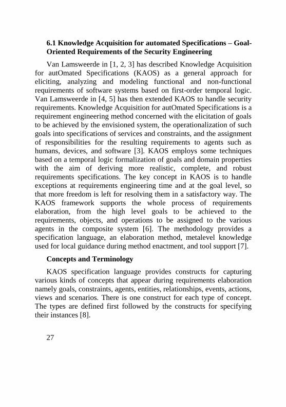
27

6.1 Knowledge Acquisition for automated Specifications – Goal-

Oriented Requirements of the Security Engineering

Van Lamsweerde in [1, 2, 3] has described Knowledge Acquisition

for autOmated Specifications (KAOS) as a general approach for

eliciting, analyzing and modeling functional and non-functional

requirements of software systems based on first-order temporal logic.

Van Lamsweerde in [4, 5] has then extended KAOS to handle security

requirements. Knowledge Acquisition for autOmated Specifications is a

requirement engineering method concerned with the elicitation of goals

to be achieved by the envisioned system, the operationalization of such

goals into specifications of services and constraints, and the assignment

of responsibilities for the resulting requirements to agents such as

humans, devices, and software [3]. KAOS employs some techniques

based on a temporal logic formalization of goals and domain properties

with the aim of deriving more realistic, complete, and robust

requirements specifications. The key concept in KAOS is to handle

exceptions at requirements engineering time and at the goal level, so

that more freedom is left for resolving them in a satisfactory way. The

KAOS framework supports the whole process of requirements

elaboration, from the high level goals to be achieved to the

requirements, objects, and operations to be assigned to the various

agents in the composite system [6]. The methodology provides a

specification language, an elaboration method, metalevel knowledge

used for local guidance during method enactment, and tool support [7].

Concepts and Terminology

KAOS specification language provides constructs for capturing

various kinds of concepts that appear during requirements elaboration

namely goals, constraints, agents, entities, relationships, events, actions,

views and scenarios. There is one construct for each type of concept.

The types are defined first followed by the constructs for specifying

their instances [8].

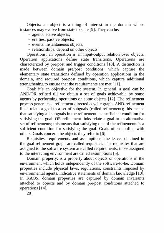
28

Objects: an object is a thing of interest in the domain whose

instances may evolve from state to state [9]. They can be:

- agents: active objects;

- entities: passive objects;

- events: instantaneous objects;

- relationships: depend on other objects.

Operations: an operation is an input-output relation over objects.

Operation applications define state transitions. Operations are

characterized by pre/post and trigger conditions [10]. A distinction is

made between domain pre/post conditions, which capture the

elementary state transitions defined by operation applications in the

domain, and required pre/post conditions, which capture additional

strengthening to ensure that the requirements are met [11].

Goal: it’s an objective for the system. In general, a goal can be

AND/OR refined till we obtain a set of goals achievable by some

agents by performing operations on some objects [12]. The refinement

process generates a refinement directed acyclic graph. AND-refinement

links relate a goal to a set of subgoals (called refinement); this means

that satisfying all subgoals in the refinement is a sufficient condition for

satisfying the goal. OR-refinement links relate a goal to an alternative

set of refinements; this means that satisfying one of the refinements is a

sufficient condition for satisfying the goal. Goals often conflict with

others. Goals concern the objects they refer to [6].

Requisites, requirements and assumptions: the leaves obtained in

the goal refinement graph are called requisites. The requisites that are

assigned to the software system are called requirements; those assigned

to the interacting environment are called assumptions [5].

Domain property: is a property about objects or operations in the

environment which holds independently of the software-to-be. Domain

properties include physical laws, regulations, constraints imposed by

environmental agents, indicative statements of domain knowledge [13].

In KAOS, domain properties are captured by domain invariants

attached to objects and by domain pre/post conditions attached to

operations [14].

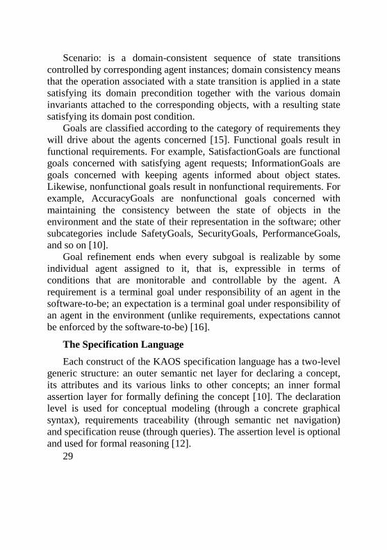
29

Scenario: is a domain-consistent sequence of state transitions

controlled by corresponding agent instances; domain consistency means

that the operation associated with a state transition is applied in a state

satisfying its domain precondition together with the various domain

invariants attached to the corresponding objects, with a resulting state

satisfying its domain post condition.

Goals are classified according to the category of requirements they

will drive about the agents concerned [15]. Functional goals result in

functional requirements. For example, SatisfactionGoals are functional

goals concerned with satisfying agent requests; InformationGoals are

goals concerned with keeping agents informed about object states.

Likewise, nonfunctional goals result in nonfunctional requirements. For

example, AccuracyGoals are nonfunctional goals concerned with

maintaining the consistency between the state of objects in the

environment and the state of their representation in the software; other

subcategories include SafetyGoals, SecurityGoals, PerformanceGoals,

and so on [10].

Goal refinement ends when every subgoal is realizable by some

individual agent assigned to it, that is, expressible in terms of

conditions that are monitorable and controllable by the agent. A

requirement is a terminal goal under responsibility of an agent in the

software-to-be; an expectation is a terminal goal under responsibility of

an agent in the environment (unlike requirements, expectations cannot

be enforced by the software-to-be) [16].

The Specification Language

Each construct of the KAOS specification language has a two-level

generic structure: an outer semantic net layer for declaring a concept,

its attributes and its various links to other concepts; an inner formal

assertion layer for formally defining the concept [10]. The declaration

level is used for conceptual modeling (through a concrete graphical

syntax), requirements traceability (through semantic net navigation)

and specification reuse (through queries). The assertion level is optional

and used for formal reasoning [12].

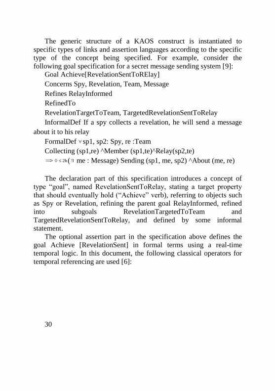
30

The generic structure of a KAOS construct is instantiated to

specific types of links and assertion languages according to the specific

type of the concept being specified. For example, consider the

following goal specification for a secret message sending system [9]:

Goal Achieve[RevelationSentToRElay]

Concerns Spy, Revelation, Team, Message

Refines RelayInformed

RefinedTo

RevelationTargetToTeam, TargetedRevelationSentToRelay

InformalDef If a spy collects a revelation, he will send a message

about it to his relay

FormalDef sp1, sp2: Spy, re :Team

Collecting (sp1,re) ^Member (sp1,te)^Relay(sp2,te)

h2 ( me : Message) Sending (sp1, me, sp2) ^About (me, re)

The declaration part of this specification introduces a concept of

type “goal”, named RevelationSentToRelay, stating a target property

that should eventually hold (“Achieve” verb), referring to objects such

as Spy or Revelation, refining the parent goal RelayInformed, refined

into subgoals RevelationTargetedToTeam and

TargetedRevelationSentToRelay, and defined by some informal

statement.

The optional assertion part in the specification above defines the

goal Achieve [RevelationSent] in formal terms using a real-time

temporal logic. In this document, the following classical operators for

temporal referencing are used [6]:

31

(in the next state) (some time in the future)

(always in the future) W (always in the future unless) B (always in the past back to)

(in the previous state) (some time in the past)

(always in the past) U (always in the future untill)

S (always in the past since)

Formal assertions are interpreted over historical sequences of states.

Each assertion is in general specified by some sequences and falsified

by some other sequences. The notation (H, i) |= P is used to express that

assertion P is satisfied by history H at time position i (i € T), where T

denotes a linear temporal structure assumed to be discrete for sake of

simplicity. Let use the notation H |= P for (H, 0) |= P.

States are global; the state of the composite system at some time

position i is the aggregation of the local states of all its objects at that

time position. The state of an individual object instance ob at some time

position is defined as a mapping from ob to the set of values of all ob’s

attributes and links at that time position. In the context of KAOS

requirements, a historical sequence of states defines a behavior

produced by a scenario [7].

The semantics of the above temporal operators is then defined as

follows [3]: (H, i)= P iff (H, next(i)) =P

(H, i)= P iff (H,j) =P for some j ≥i

(H, i)= P iff (H,j) =P for all j ≥i

(H, i)= PUQ iff there exists a j≠I such that (H, i)=Q and for every k, i≤k<j, (H,k) =P

(H, i)= PWQ (H,i) =PUQ or (H,i) = P

(H, i)= PSQ iff there exists a j≤I such that (H, i)=Q and for every k, i<k≤j, (H,k) =P

(H, i)= PBQ (H,i) = PSQ or (H,i) = P

Note that P amounts to PW false. Let use the standard logical

connectives (and), (or), (not), (implies), (equivalent),

(strongly implies), (strongly equivalent), with

32

Note thus that there is an implicit outer operator in every strong

implication. Beside the agent-related classification of goals, goals in

KAOS are also classified according to the pattern of temporal behavior

they capture:

Achieve: C T

Cease: C T

Maintain: C TWN, C TWN

Avoid: C TWN, C T

In these patterns, C, T, and N denote some current, target, and new

condition respectively. In requirements engineering, it is needed to

introduce real-time restrictions. Bounded versions of the above

temporal operators are therefore introduced in the following style: ≤ d (some time in the future within deadline d)

≤ d (always in the future up to deadline d)

To define such operators, the temporal structure T is enriched with

a metric domain D and a temporal distance function dist: T x T D,

which has all desired properties of metrics. We will take:

T: the set of naturals

D: {d there exists a natural n such that d=n×u}, where

u denotes some chosen tin}

dist(i,j): j-i × u

Multiple units can be used – e.g., s (second), m (minute), d (day),

etc; these are implicitly converted into some smaller unit. The o-

operator then yields the nearest subsequent time position according to

this smallest unit.

The semantics of the real-time operators is then defined

accordingly, e.g.,

33

(H, i)= ≤ d P iff (H,j) =P for some j ≠i with dist(i,j)≤d

(H, i)= ≤ d P iff (H,j) =P for all j ≠i such that dist(i,j)<d In the above goal declaration of RevelationSentToRelay, the

conjunction of the assertions formalizing the subgoals

RevelationTargetedToTeam and TargetedRevelationSentToRelay must

entail the formal assertion of the parent goal RevelationSent they define

together. Every formal goal refinement thus generates a corresponding

proof obligation [13].

In the formal assertion of the goal RevelationSentToRelay, the

predicate Sending(sp1, me, sp2) means that, in the current state, an

instance of the Sending relationship links variables sp1, me, and sp2 of

sort Spy, Revelation, respectively. The Sending relationship and

Revelation entity are defined in such a way:

Entity Revalation InformalDef Secret information about the enemy

Has Content: Text

Relationship Sending InformalDef A spy is sending a message to another spy

Links Spy {Role Sends} Message {Role Sent}

Spy{Role To} The Spy type might in turn be declared by

Agent Spy InformalDef Person who is an employee of the a spy agency

Has Name: Text In the declarations above, Name is declared as an attribute of the

entity Spy.

As mentioned earlier, operations may be specified formally by pre

and post conditions in the state-based style, e.g.,

34

Operation Send Relevation Input Spy {arg sp1, sp2}, Revelation {arg re}

Output Message {res me}, Sending DomPre ( me: Message) Sending (sp1,me,sp2) DomPost ( me: Message) Sending (sp1,me,sp)

The pre and post condition of the operation SendRevelation above

are domain properties; they capture corresponding elementary state

transitions in the domain, namely, from a state where no message is

sent to a state where a message is sent. The software requirements are

found in the terminal goals assigned to agents in the software-to-be, and

in the additional pre, post and trigger conditions that need to strengthen

the corresponding domain conditions in order to ensure all such goals.

Assuming the RevelationSentToRelay goal is assigned to the spy

collecting the revelation one would derive from the above formal

assertion for that goal:

Operation SendRevelation …

ReqTrigFor RevelationSent Collecting (sp1, re)

ReqPreFor RevelationSent ( te: Team) Member (sp1, te) ^Relay (sp2,te)

ReqPostFor RevelationSent About (me,re)

The trigger condition captures an obligation to trigger the operation

as soon as the condition gets true and provided the domain precondition

is true. The specification will be consistent provided the trigger

condition and required precondition are together true in the operation’s

initial state.

The Elaboration Method

Figure 6.1 outlines the major steps that may be followed to

elaborate KAOS specifications from high-level goals.

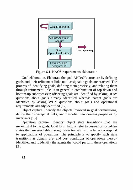
35

Figure 6.1. KAOS requirements elaboration

Goal elaboration. Elaborate the goal AND/OR structure by defining

goals and their refinement links until assignable goals are reached. The

process of identifying goals, defining them precisely, and relating them

through refinement links is in general a combination of top-down and

bottom-up subprocesses; offspring goals are identified by asking HOW

questions about goals already identified whereas parent goals are

identified by asking WHY questions about goals and operational

requirements already identified [12].

Object capture. Identify the objects involved in goal formulations,

define their conceptual links, and describe their domain properties by

invariants [13].

Operation capture. Identify object state transitions that are

meaningful to the goals. Goal formulations refer to desired or forbidden

states that are reachable through state transitions; the latter correspond

to applications of operations. The principle is to specify such state

transitions as domain pre- and post conditions of operations thereby

identified and to identify the agents that could perform these operations

[3].

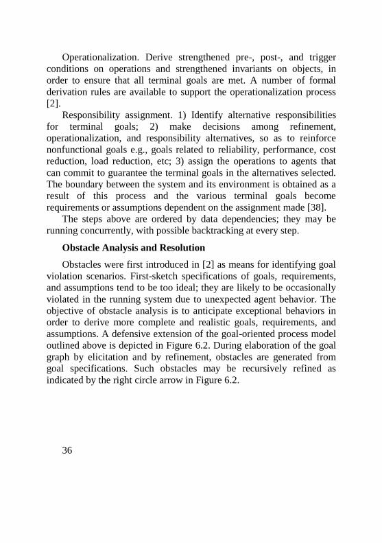
36

Operationalization. Derive strengthened pre-, post-, and trigger

conditions on operations and strengthened invariants on objects, in

order to ensure that all terminal goals are met. A number of formal

derivation rules are available to support the operationalization process

[2].

Responsibility assignment. 1) Identify alternative responsibilities

for terminal goals; 2) make decisions among refinement,

operationalization, and responsibility alternatives, so as to reinforce

nonfunctional goals e.g., goals related to reliability, performance, cost

reduction, load reduction, etc; 3) assign the operations to agents that

can commit to guarantee the terminal goals in the alternatives selected.

The boundary between the system and its environment is obtained as a

result of this process and the various terminal goals become

requirements or assumptions dependent on the assignment made [38].

The steps above are ordered by data dependencies; they may be

running concurrently, with possible backtracking at every step.

Obstacle Analysis and Resolution

Obstacles were first introduced in [2] as means for identifying goal

violation scenarios. First-sketch specifications of goals, requirements,

and assumptions tend to be too ideal; they are likely to be occasionally

violated in the running system due to unexpected agent behavior. The

objective of obstacle analysis is to anticipate exceptional behaviors in

order to derive more complete and realistic goals, requirements, and

assumptions. A defensive extension of the goal-oriented process model

outlined above is depicted in Figure 6.2. During elaboration of the goal

graph by elicitation and by refinement, obstacles are generated from

goal specifications. Such obstacles may be recursively refined as

indicated by the right circle arrow in Figure 6.2.

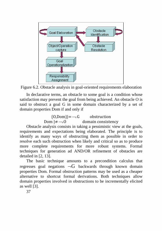
37

Figure 6.2. Obstacle analysis in goal-oriented requirements elaboration

In declarative terms, an obstacle to some goal is a condition whose

satisfaction may prevent the goal from being achieved. An obstacle O is

said to obstruct a goal G in some domain characterized by a set of

domain properties Dom if and only if

{O,Dom}|=G obstruction Dom |≠O domain consistency

Obstacle analysis consists in taking a pessimistic view at the goals,

requirements and expectations being elaborated. The principle is to

identify as many ways of obstructing them as possible in order to

resolve each such obstruction when likely and critical so as to produce

more complete requirements for more robust systems. Formal

techniques for generation ad AND/OR refinement of obstacles are

detailed in [2, 13].

The basic technique amounts to a precondition calculus that

regresses goal negations G backwards through known domain

properties Dom. Formal obstruction patterns may be used as a cheaper

alternative to shortcut formal derivations. Both techniques allow

domain properties involved in obstructions to be incrementally elicited

as well [3].

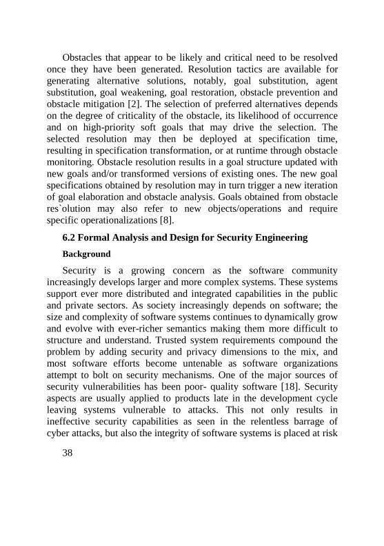
38

Obstacles that appear to be likely and critical need to be resolved

once they have been generated. Resolution tactics are available for

generating alternative solutions, notably, goal substitution, agent

substitution, goal weakening, goal restoration, obstacle prevention and

obstacle mitigation [2]. The selection of preferred alternatives depends

on the degree of criticality of the obstacle, its likelihood of occurrence

and on high-priority soft goals that may drive the selection. The

selected resolution may then be deployed at specification time,

resulting in specification transformation, or at runtime through obstacle

monitoring. Obstacle resolution results in a goal structure updated with

new goals and/or transformed versions of existing ones. The new goal

specifications obtained by resolution may in turn trigger a new iteration

of goal elaboration and obstacle analysis. Goals obtained from obstacle

res`olution may also refer to new objects/operations and require

specific operationalizations [8].

6.2 Formal Analysis and Design for Security Engineering

Background

Security is a growing concern as the software community

increasingly develops larger and more complex systems. These systems

support ever more distributed and integrated capabilities in the public

and private sectors. As society increasingly depends on software; the

size and complexity of software systems continues to dynamically grow

and evolve with ever-richer semantics making them more difficult to

structure and understand. Trusted system requirements compound the

problem by adding security and privacy dimensions to the mix, and

most software efforts become untenable as software organizations

attempt to bolt on security mechanisms. One of the major sources of

security vulnerabilities has been poor- quality software [18]. Security

aspects are usually applied to products late in the development cycle

leaving systems vulnerable to attacks. This not only results in

ineffective security capabilities as seen in the relentless barrage of

cyber attacks, but also the integrity of software systems is placed at risk

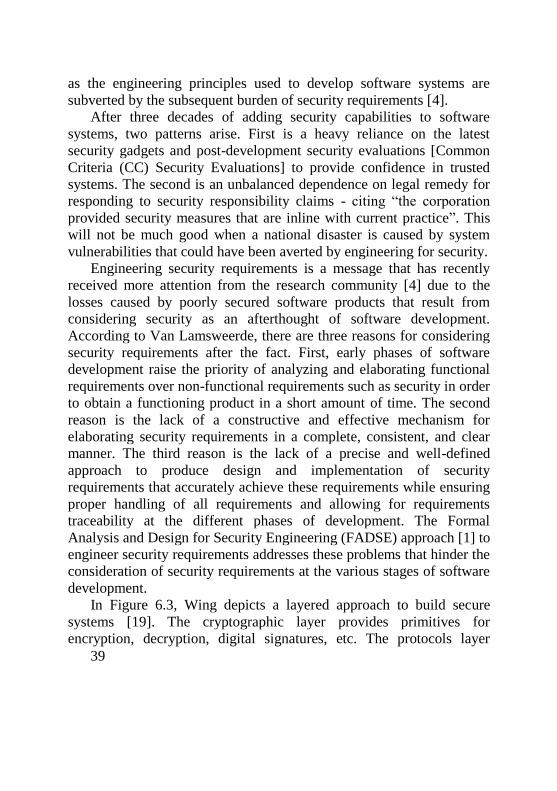
39

as the engineering principles used to develop software systems are

subverted by the subsequent burden of security requirements [4].

After three decades of adding security capabilities to software

systems, two patterns arise. First is a heavy reliance on the latest

security gadgets and post-development security evaluations [Common

Criteria (CC) Security Evaluations] to provide confidence in trusted

systems. The second is an unbalanced dependence on legal remedy for

responding to security responsibility claims - citing “the corporation

provided security measures that are inline with current practice”. This

will not be much good when a national disaster is caused by system

vulnerabilities that could have been averted by engineering for security.

Engineering security requirements is a message that has recently

received more attention from the research community [4] due to the

losses caused by poorly secured software products that result from

considering security as an afterthought of software development.

According to Van Lamsweerde, there are three reasons for considering

security requirements after the fact. First, early phases of software

development raise the priority of analyzing and elaborating functional

requirements over non-functional requirements such as security in order

to obtain a functioning product in a short amount of time. The second

reason is the lack of a constructive and effective mechanism for

elaborating security requirements in a complete, consistent, and clear

manner. The third reason is the lack of a precise and well-defined

approach to produce design and implementation of security

requirements that accurately achieve these requirements while ensuring

proper handling of all requirements and allowing for requirements

traceability at the different phases of development. The Formal

Analysis and Design for Security Engineering (FADSE) approach [1] to

engineer security requirements addresses these problems that hinder the

consideration of security requirements at the various stages of software

development.

In Figure 6.3, Wing depicts a layered approach to build secure

systems [19]. The cryptographic layer provides primitives for

encryption, decryption, digital signatures, etc. The protocols layer

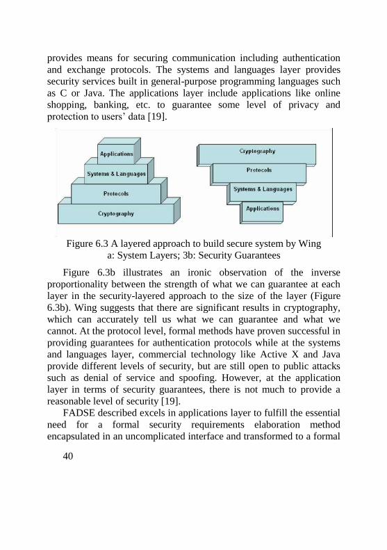
40

provides means for securing communication including authentication

and exchange protocols. The systems and languages layer provides

security services built in general-purpose programming languages such

as C or Java. The applications layer include applications like online

shopping, banking, etc. to guarantee some level of privacy and

protection to users’ data [19].

Figure 6.3 A layered approach to build secure system by Wing

a: System Layers; 3b: Security Guarantees

Figure 6.3b illustrates an ironic observation of the inverse

proportionality between the strength of what we can guarantee at each

layer in the security-layered approach to the size of the layer (Figure

6.3b). Wing suggests that there are significant results in cryptography,

which can accurately tell us what we can guarantee and what we

cannot. At the protocol level, formal methods have proven successful in

providing guarantees for authentication protocols while at the systems

and languages layer, commercial technology like Active X and Java

provide different levels of security, but are still open to public attacks

such as denial of service and spoofing. However, at the application

layer in terms of security guarantees, there is not much to provide a

reasonable level of security [19].

FADSE described excels in applications layer to fulfill the essential

need for a formal security requirements elaboration method

encapsulated in an uncomplicated interface and transformed to a formal

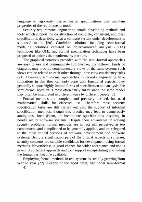
41

language to rigorously derive design specifications that maintain

properties of the requirements model.

Security requirements engineering entails developing methods and

tools which support the construction of complete, consistent, and clear

specifications describing what a software system under development is

supposed to do [20]. Candidate solutions including semi-formal

modeling notations centered on object-oriented analysis (OOA)

techniques like UML and formal specification techniques have been

proposed to address the requirements problem.

The graphical notations provided with the semi-formal approaches

are easy to use and communicate [3]. Further, the different kinds of

diagrams may provide complementary views of the same system; such

views can be related to each other through inter-view consistency rules

[21]. However, semi-formal approaches to security engineering have

limitations in that they can only cope with functional aspects; they

generally support highly limited forms of specification and analysis; the

semi-formal notation is most often fairly fuzzy since the same model

may often be interpreted in different ways by different people [3].

Formal methods are complete and precisely defined, but need

mathematical skills for effective use. Therefore most security

specification tasks are still carried out with the support of informal

specification methods, though this practice may lead to dangerously

ambiguous, inconsistent, or incomplete specifications resulting in

poorly secure software systems. Despite their advantages in solving

security problems, formal methods are in fact still perceived as too

cumbersome and complicated to be generally applied, and are relegated

to the most critical sections of software development and software

systems. Being a signification part of the critical aspects in software,

security concerns are suitable candidates for development using formal

methods. Nevertheless, a good chance for wider acceptance and use is

given, if sufficient approach and tool support encapsulating and hiding

the formal part become available.

Employing formal methods in real systems is steadily growing from

year to year [22]. Despite of the good news, traditional semi-formal

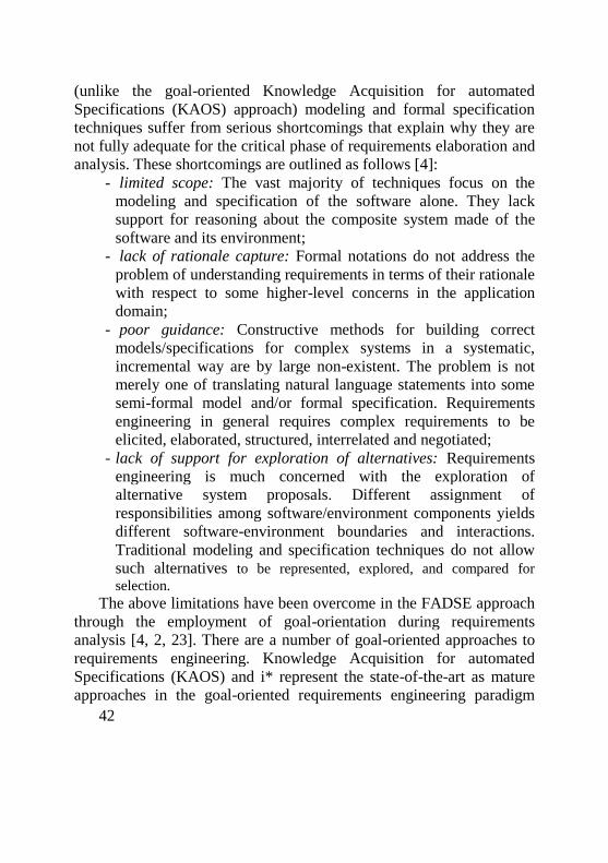
42

(unlike the goal-oriented Knowledge Acquisition for automated

Specifications (KAOS) approach) modeling and formal specification

techniques suffer from serious shortcomings that explain why they are

not fully adequate for the critical phase of requirements elaboration and

analysis. These shortcomings are outlined as follows [4]:

- limited scope: The vast majority of techniques focus on the

modeling and specification of the software alone. They lack

support for reasoning about the composite system made of the

software and its environment;

- lack of rationale capture: Formal notations do not address the

problem of understanding requirements in terms of their rationale

with respect to some higher-level concerns in the application

domain;

- poor guidance: Constructive methods for building correct

models/specifications for complex systems in a systematic,

incremental way are by large non-existent. The problem is not

merely one of translating natural language statements into some

semi-formal model and/or formal specification. Requirements

engineering in general requires complex requirements to be

elicited, elaborated, structured, interrelated and negotiated;

- lack of support for exploration of alternatives: Requirements

engineering is much concerned with the exploration of

alternative system proposals. Different assignment of

responsibilities among software/environment components yields

different software-environment boundaries and interactions.

Traditional modeling and specification techniques do not allow

such alternatives to be represented, explored, and compared for

selection. The above limitations have been overcome in the FADSE approach

through the employment of goal-orientation during requirements

analysis [4, 2, 23]. There are a number of goal-oriented approaches to

requirements engineering. Knowledge Acquisition for automated

Specifications (KAOS) and i* represent the state-of-the-art as mature

approaches in the goal-oriented requirements engineering paradigm

43

[24]. KAOS, the more well- established of the two, uses first-order

temporal logic as its formal infrastructure with good tool support [23].

Further, KAOS is unique in its conceptual ontology: lower level

descriptions of the system-to-be are progressively derived from system-

level and organizational objectives using a framework that is essentially

a taxonomy of concepts instantiated for a particular domain [25].

The KAOS security extension employed in FADSE to model and

analyze security requirements meet a set of meta-requirements that

make such model securely reliable as follows [4]:

- early deployment: In view of the criticality of security

requirements, the technique is applicable as early as possible in

the requirement engineering process, that is, to declarative

assertions as they arise from stakeholder interviews and

documents (as opposed to, e.g., later state machine models);

- incrementality: This technique supports the intertwining of

model building and analysis and therefore allow for reasoning

about partial models;

- reasoning about alternatives: This technique makes it possible to

represent and assess alternative options so that a “best” route to

security can be selected;

- high assurance: This technique allows for formal analysis when

and where needed so that compelling evidence of security

assurance can be provided;

- security-by-construction: To avoid the endless cycle of defect

fixes generating new defects, the requirements engineering

process is guided so that a satisfactory level of security is

guaranteed by construction;

- separation of concerns: This technique keeps security

requirements separate from other types of requirements so as to

allow for interaction analysis.

FADSE is the first to extend the goal-oriented KAOS framework to

formal design and implementation, which brings the benefits of the

goal-oriented paradigm to the software security domain. The

employment of goal-orientation prior to stepping into formal design

44

paves the road for formal design through performing thorough

reasoning about security requirements and organizing them into a well-

structured requirements model. Van Lamsweerde argues that goals

offer the right kind of abstraction to address the inadequacies of formal

and semi-formal methods for requirements engineering (especially for

high assurance systems). These systems require compelling evidence

that they deliver their services in a manner that satisfies safety, security,

fault-tolerance and survivability requirements.

Goal-oriented methods are adequate for requirements engineering

that is concerned with the elicitation of goals to be achieved by the

software-to-be (WHY issues), the operationalization of such goals into

specifications of services and constraints (WHAT issues), and the

assignment of responsibilities for the resulting requirements to agents

such as humans, devices and software available or to be developed

(WHO issues) [26]. Positive/negative interactions with the other system

goals can be captured in goal models and managed appropriately [2];

exceptional conditions in the environment that might hinder critical

goals from being achieved can be identified and resolved to produce

more robust requirements [2]; the goals can be specified precisely and

refined incrementally into operational software specifications that

provably assure the higher-level goals [8, 7, 11]. Requirements

implement goals much the same way as programs implement design

specifications [4].

Most research efforts in the field of security requirements

engineering have been devoted to the requirements specification facet

of requirements engineering [14]. A large number of languages have

been proposed for requirements specifications, some of which are

popular formal languages like Z, VDM, or LARCH. However, these

languages are not well suited for capturing requirements models

because they are too restricted in scope; they address only the “what”

questions [11]. Typically, the data and operations of the system

envisioned are specified through first-order assertions like conditional

equations or pre/postconditions and invariants. Another limitation is

that such languages have no built-in constructs for making a clear

45

separation between domain descriptions and actual requirements [14].

Van Lamsweerde indicated that recent attempts to design semi-formal

languages like KAOS support a wider range of requirements with the

ability to address the “why”, “who”, and “when” questions in addition

to the normal “what” questions [14].

FADSE addresses the limitations of the security requirements

specification languages through employing KAOS to elicit security

requirements that uses first order temporal logic to formally capture

pre, post conditions and domain invariants. Moreover, KAOS models

security aspects as goals resulting in a security goal graph in which the

bottom level goals are either security requirements assigned to agents in

the software-to-be (the software whose requirements are being

modeled) or assumptions to be fulfilled by the interacting environment.

This differentiation between requirements and assumptions clearly

separates domain descriptions from actual requirements. Further, the

bottom level goals of the graph are goals to be assigned to agents

allowing the requirements model to extend beyond answering what

questions to answer how questions and who is responsible for achieving

these goals.

Being a crucial aspect in system development, security must be

thoroughly ensured during all development phases. While still mostly

relegated to the implementation and testing phases, it should be

enforced at earlier stages too, i.e. in the requirements elaboration phase

since early detection of possible security vulnerabilities is a key factor

towards developing secure systems that are cost effective. Again,

FADSE is a requirements-driven approach that considers security very

early in development while security vulnerabilities are analyzed and

resolved. Moreover, the rest of the development phases are guided

requirements model using the B formal method refinement mechanism

that obtains its initial B model from automatically transforming the

KAOS model to B. The employment of B as a design elaboration

method to fully develop security-specific elements of software allows

for the automatic verification of security implementation from more

abstract properties represented in the requirements model. Further, the

46

derivation of acceptance test cases from the requirements model

provides means to ensure compliance between the derived

implementation and the initial set of security requirements.

Automatic code generation from requirements facilitates the

production of large systems with high- quality in a cost-effective

manner. Therefore, it has been one of the objectives of software

engineering almost since the advent of high-level programming

languages, and calls for a “requirements-based programming”

capability has become deafening [27]. Several tools and products exist

in the marketplace for automatic code generation from a given model.

However, they typically generate code, portions of which are never

executed, or portions of which cannot be justified from either the

requirements or the model [27]. Moreover, existing tools do not and

cannot overcome the fundamental inadequacy of all currently available

automated development approaches, which is that they include no

means to establish a provable equivalence between the requirements

stated at the outset and either the model or the code they generate.

FADSE solves this problem by building a mature and formally

analyzed security requirements model using KAOS and transforms this

requirements model into B to fully develop security aspects.

Discharging B proof obligations provides means to establish a provable

equivalence between the security requirements model and the more

specified models produced for design and implementation.

While security-in-the-large encompasses development, deployment,

and administration of trusted systems in their operational environments,

this research focuses largely on the development process. We

conjecture that purposefully engineering security principles into trusted

systems during development reduces the risks of manifesting

vulnerabilities during deployment, administration, and operation in the

trusted environment. More concisely, while well understood security

principles exist to guide organizations and security best practices exist

for specific areas of development, there is no cohesive framework of

security engineering principles that integrates development activities,

artifacts, and practices, with relevant security principles. Lacking an

47

integrated software security engineering process that incorporates

security principles from the onset, we continue to employ informal

solutions that render many subsequent systems vulnerable to attacks.

From the perspective of building a system devoid of security

vulnerabilities, formal methods have been hoisted up as a reasonable

solution. However, formal methods come with some challenges for

large, complex systems. First, the application of formal methods entails

substantial requirements formulation in a precise provable and correct

representation, unambiguous, and consistent. Even for moderate

systems, this goal is not readily achieved from a cost and time

perspective. Secondly, once formal requirements set exists, translating

them into a design that preserves the requisite security properties can be

arduous and error-prone and arduous. Thirdly, the availability of

engineers with the requisite experience to render a system definition

and design specification formally is relatively low and they are often

more expensive to employ.

Combining the increasing need for secure systems and the

challenges of formal methods-based solutions, we have a dilemma. Do

we bite the bullet and apply formal methods to engineering secure

systems or do we continue down the informal path and live with the

resulting vulnerabilities? This approach leads us to believe that there is

a rational middle ground. First, assuring that all vulnerabilities are

covered is unrealistic both technically and economically unless we are

willing to accept systems of low size and complexity. Secondly,

requirements engineering with formal methods is precise and provides a

good platform for better completeness, but it still lacks the guarantees

that completeness is achieved. Therefore, the argument for

completeness turns to a tradeoff between approaches for time taken for

getting to an acceptable level of completeness before proceeding on to

design.

The requirements-driven goal-directed FADSE approach proposed

as a step towards the development of highly secure software is less

precise and formal than starting from a totally formal approach, but it

has three key mechanisms that render near-formal results. First, it

48

employs KAOS (Knowledge Acquisition for autOmated Specifications)

[4, 2], which is a proven goal-directed framework to elaborate security

requirements. KAOS is natural for identifying and reasoning about the

requisite requirements - making it an effective mechanism for

facilitating completeness with additional formality in areas where it is

essential. Second, the obstacle analysis mechanism of KAOS provides a

good capability to reduce the presence of vulnerabilities by

concentrating on the most appropriate alternatives for avoiding or

eliminating the obstacles. Third, the test-case generation from the

requirements model assures better alignment with the requirements and

confidence in the specification from a verifiability perspective.

FADSE might have a broader impact in two dimensions. The first is

that it could enhance the infrastructure for research as some of the case

studies used to demonstrate and verify the approach are industry-

oriented. This collaboration between the proposed work and industry

broadens its impact and extends its applicability and practicality. The

second dimension in which FADSE has a broader impact is that it

widens dissemination to enhance scientific and technological

understanding. This is achieved through the results obtained from

verifying the approach through a controlled experiment, which are

beneficial to software engineers in general and to security engineers in

specific who lack a constructive and systematic approach to capture and

develop security concerns in software products.

State of the Art Survey

FADSE is a security engineering approach employing formal

methods to analyze, design and implement security-specific elements of

software with the aim of producing highly secured software products.

FADSE can therefore be positioned in the intersection of three areas of

software research namely software engineering, security and formal

methods as illustrated in Figure 6.4. This chapter surveys research

efforts of employing formal methods to produce highly secured

software, elaborating and modeling security requirements, deriving

design specifications and implementation from requirements using

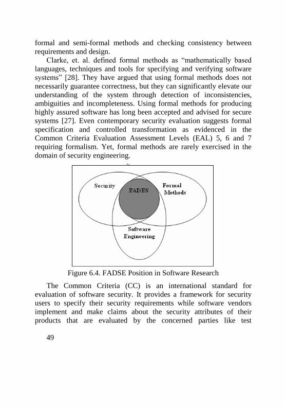
49

formal and semi-formal methods and checking consistency between

requirements and design.

Clarke, et. al. defined formal methods as “mathematically based

languages, techniques and tools for specifying and verifying software

systems” [28]. They have argued that using formal methods does not

necessarily guarantee correctness, but they can significantly elevate our

understanding of the system through detection of inconsistencies,

ambiguities and incompleteness. Using formal methods for producing

highly assured software has long been accepted and advised for secure

systems [27]. Even contemporary security evaluation suggests formal

specification and controlled transformation as evidenced in the

Common Criteria Evaluation Assessment Levels (EAL) 5, 6 and 7

requiring formalism. Yet, formal methods are rarely exercised in the

domain of security engineering.

Figure 6.4. FADSE Position in Software Research

The Common Criteria (CC) is an international standard for

evaluation of software security. It provides a framework for security

users to specify their security requirements while software vendors

implement and make claims about the security attributes of their

products that are evaluated by the concerned parties like test

50

laboratories to verify the claims. The CC defines seven Evaluation

Assurance Levels (EAL 1 to EAL 7) to measure the degree of

compliance between the product and the claimed security functionality.

Each EAL covers the complete development of a product with a given

level of strictness with EAL 1 being the most basic and hence the

cheapest to implement and evaluate and EAL 7 being the most rigorous

and expensive [29]. The first four EAL levels of the CC do not require

formal evidence for assuring the security functionality of the products

while EAL levels 5, 6 and 7 have requisites of providing formal

artifacts of development to assure the claimed security attributes. This

means that products assured at EAL 5-7 provides more confidence to

the users in the security claims of the product.

EAL1 is applicable where some confidence in correct operation is

mandated while security threats are not considered serious [29].

Evaluation at EAL1 should show evidence of compliance between the

target of evaluation functions and its documentation using, for example,

testing. EAL2 requires the interference of the developers in delivering

design and test results and is applicable where low to moderate level of

security is required. EAL2 provides security assurance by analyzing the

security functions using requirements specifications, guidance

documentation and the high-level design of the target of evaluation

[29]. EAL3 thoroughly investigate the target of evaluation without

substantial re-engineering. EAL3 provides security assurance using

requirements specifications, documentation and the high level design;

however, the analysis is supported by testing of security functions and

evidence of the developer testing. EAL4 is applicable to moderate and

high level security and it provides assurance through analysis of

security functions using complete requirements specifications,

documentation, high-level and low-level design, and subset of the

implementation to understand security behavior [29].

EAL5 is the first assurance level requiring formal evidence of

development to assure high-level security of the target of evaluation.

EAL5 requires complete specification, documentation, high-level and

low-level designs and all of the implementation. Assurance is further

51

gained through a formal model of the security policy and a semi-formal

presentation of the requirements specifications and the high-level

design and a semi-formal evidence of the compliance between the two.

EAL6 gains assurance through a formal model of security, a

semiformal presentation of the security requirements specifications,

high-level and low-level designs and a semiformal evidence of the

compliance between the specifications and the two designs. Further, a

modular and layered design is required. EAL7 is applicable to

extremely high-risk applications where the assets need maximum

protection. EAL7 assures security through a formal model of the

security policy, formal presentation of the security requirements

specifications, high-level design, a semiformal presentation of the low-

level design and formal and semiformal evidence of compliance

between specifications and both the high-level and low-level designs.

These definitions imply that the software products developed with

FADSE could be assured at EAL5, EAL6 and EAL7. These three

evaluation assurance levels especially EAL6 require semiformal

presentation of the requirements specifications, which are provided in

FADSE in the semiformal form of the KAOS goal graph. Further,

EAL6 and EAL7 require formal presentation of design, which is

provided in FADSE using the B formal method and a semiformal

evidence of compliance between specifications and design, which is

provided in FADSE using the acceptance test cases generated from the

specifications model (KAOS goal graph). The employment of formal

methods in FADSE provides the required formal evidence of

development for the assurance of the resulting target of evaluation at

EAL5-7.

There are a number of success stories for applying formal methods

to security-critical systems at the application layer; however, there are

few if any formal methods-based approaches that handle security-

specific elements. Stepney used the Z formal language to construct a

security requirements specifications model that has been further refined

to derive design and implementation specifications for a money

exchange system using smart cards [30]. Clarke surveyed several

52

applications of formal methods to security aspects [28]. Oxford

University and IBM Hursley Laboratories collaborated in the 1980s on

employing Z to formalize part of IBM’s Customer Information Control

System (CICS), an online transaction processing system with thousands

of installations worldwide [28]. IBM reported measurements collected

throughout development to indicate an overall improvement in product

quality, a reduction in the number of errors discovered, earlier detection

of errors, and an estimated 9% reduction in total development cost.

Sabatier and Lartigue reported on industrial smart card application in

which they designed the transaction mechanism to provide secure

means for modifying data that is permanently stored in smart cards

[31]. They demonstrated how the use of the B method increased

confidence and provided mathematical proof that the design of the

transaction mechanism fulfills the security requirements.

A number of approaches have been proposed in the literature for

elaborating and modeling security requirements in a way comparable

FADSE. Misuse cases that complement UML are able to capture

attacker features at requirements engineering time. Misuse cases are

defined as “the inverse of UML use cases specifying functions that the

system should not allow” [32, 33]. Misuse cases refer to scenarios that

result in loss for the organization or some specific stakeholder. The

concept of mis-actor is associated with the misuse cases. A mis-actor is

defined as “the inverse of a UML actor, who is someone-intentionally

or accidentally initiates misuse cases and whom the system should not

support in doing so” [32]. Misuse cases can be normally related to

normal use cases through “includes”, “extends”, “prevents”, and

“detects” relations. The relation of “includes” or “extends” from a

misuse case to an ordinary use case indicates a misuse of one of the

functions of the ordinary use cases. For example, a denial of service

(DoS) attack needs not include illegal actions, just flooding the system

with a heavy burden of publicly available registration requests. The

“prevents” and “detects” have been introduced specifically for misuse

cases, which relate ordinary uses cases to misuse cases outlining

functions that prevent or detect misuse [32].

53

Firesmith in [34] has differentiated between misuse cases and

security use cases. Firesmith thinks that misuse cases provide means for

analyzing security threats but are inappropriate for the analysis and

specification of security requirements. Instead, security use cases

should define possible threat scenarios from which the application

should be protected. Figure 6.5 shows the functionality of both misuse

cases and security use cases. Security use cases could then be integrated

with the rest of UML artifacts such as class and interaction diagrams in

order to provide a software engineering approach that captures security

requirements early on and integrates them with the rest of the system

development phases through UML [34].

Unlike FADSE, misuse cases and security requirements use cases

handle security concerns only during the requirements and analysis

phases while FADSE covers the different stages of development for

security requirements to produce a complete implementation. Misuse

cases and security use cases inherit the simplicity and popularity as well

as the semantic inconsistencies of UML. Further, they lack the rigor

and requirements traceability features in FADSE.

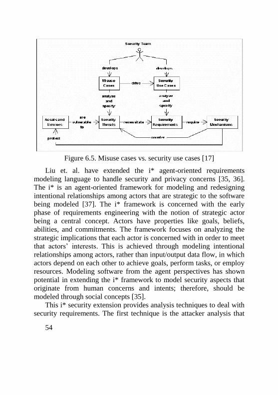
54

Figure 6.5. Misuse cases vs. security use cases [17]

Liu et. al. have extended the i* agent-oriented requirements

modeling language to handle security and privacy concerns [35, 36].

The i* is an agent-oriented framework for modeling and redesigning

intentional relationships among actors that are strategic to the software

being modeled [37]. The i* framework is concerned with the early

phase of requirements engineering with the notion of strategic actor

being a central concept. Actors have properties like goals, beliefs,

abilities, and commitments. The framework focuses on analyzing the

strategic implications that each actor is concerned with in order to meet

that actors’ interests. This is achieved through modeling intentional

relationships among actors, rather than input/output data flow, in which

actors depend on each other to achieve goals, perform tasks, or employ

resources. Modeling software from the agent perspectives has shown

potential in extending the i* framework to model security aspects that

originate from human concerns and intents; therefore, should be

modeled through social concepts [35].

This i* security extension provides analysis techniques to deal with

security requirements. The first technique is the attacker analysis that

55

identifies potential system attacks. The attacker analysis theme is that

“all actors are assumed guilty until proven innocent” [35]. Ordinary

system actors (roles, positions or agents) are considered among

potential attackers to the system or to other actors. The second analysis

technique is the dependency vulnerability analysis that detects

vulnerabilities in terms of organizational relationships among

stakeholders whose dependency relationships bring vulnerabilities to

actually attack the system through the manipulation of their malicious

intents. Detailed analysis of vulnerability with the i* dependency

modeling capability to trace the potential failure of each dependency to

a dependent and to its dependents. Countermeasure analysis proposes

proactive actions to resolve vulnerabilities and threats. Finally, access

control analysis fills in the gap between security requirements and their

realization in implementation. Access control analysis uses i* models to

embed a proposed solution to system design. The i* role-based

requirements analysis with i* facilitates the transition from

requirements to design since it fits naturally to the role-based access

control methodology software design.

The i* security extension is close in spirit to KAOS security

extension employed in FADSE. The main difference is that the i*

security extension starts with agents involved in the system rather than

goals being threatened as in KAOS. Further, the i* security extension

identifies insider attackers only, that is, system stakeholders that were

identified before in the primal model and might be suspect while KAOS

identifies possible attacks regardless they can be performed by insider

or outsider attackers. In the i* security extension, the malicious goals

owned by attackers are not modeled explicitly and the methodology

provides no formal techniques for building threat models. On the other

hand, the KAOS security extension provides a formal procedure for

generating attacks and countermeasure to such attacks, which makes

KAOS more reliable especially in the security requirements context.

Both the KAOS security extension and the i* security extension

provide constructs to effectively reason about security requirements.

However, the KAOS security extension has been favored over the i*

56

one to employ in FADSE because the i* framework is not based on

first-order predicate logic like KAOS making it difficult to transform to

a formal language like B.

There are a number of approaches proposed in the domain of

deriving design from requirements both formally and semi-formally.

Some of these approaches extended the KAOS framework for further

stages in development like architecture and design. All the approaches

that extended KAOS exploited the key features of goal-orientation

namely the ability to explore alternatives in specifications,

responsibility assignment, goal formalization, adapting different levels

of formality, and modeling the software and its environment. However,

the approaches that extended KAOS focused on the functional and non-

functional requirements of the system and none of them addressed the

security aspects like FADSE. This distinguishes FADSE in being the

first to employ goal-orientation for the design and implementation of

security-specific aspects of software system.

Nekagawa et. al. have proposed a formal specification generator

that transforms KAOS requirements specifications into VDM++

specifications to develop software systems [38]. Requirements are

elaborated and analyzed using KAOS resulting in the construction of a

requirements model, which is given as an input to the generator to

produce the VDM++ specification. Missing parts in the requirements

model are commented during the generation process to prompt

developers to augment the VDM++ specification. The generated

specification contains implicit operations consisting of pre and post-

conditions, inputs, and outputs while the body of operations is left for

developers to add to create an explicit specification. Test cases are

developed to verify the formal specification using the VDM tools [38].

An overview of the VDM++ generator steps and artifacts is illustrated

in Figure 6.6. Like FADSE, the VDM++ generator formally derives

design from requirements modeled with KAOS. Nevertheless, the

VDM++ generator only derives high level design with no specific focus

on security aspects.

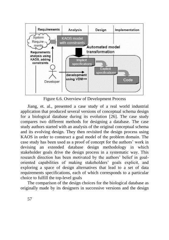
57

Figure 6.6. Overview of Development Process

Jiang, et. al., presented a case study of a real world industrial

application that produced several versions of conceptual schema design

for a biological database during its evolution [26]. The case study

compares two different methods for designing a database. The case

study authors started with an analysis of the original conceptual schema

and its evolving design. They then revisited the design process using

KAOS in order to construct a goal model of the problem domain. The

case study has been used as a proof of concept for the authors’ work in

devising an extended database design methodology in which

stakeholder goals drive the design process in a systematic way. This

research direction has been motivated by the authors’ belief in goal-

oriented capabilities of making stakeholders’ goals explicit, and

exploring a space of design alternatives that lead to a set of data

requirements specifications, each of which corresponds to a particular

choice to fulfill the top-level goals

The comparison of the design choices for the biological database as

originally made by its designers in successive versions and the design

58

recommendations suggested by the goal analysis shows that the goal-

driven approach results in a design spaces that:

- includes original schema built through the evolution of the

application;

- suggests additional alternatives that lead to more comprehensive

design;

- supports systematic evaluation of design alternatives;

- generates schemas with rich and explicit data semantics.

The authors’ interpretation to the above results is that goal analysis

allows the cognitive process that took place in the actual design of the

database to be explicit when goals are declared as opposed to being

implicit in the traditional method [26]. This led to schema design that

better responds to the purpose of the application. The schema resulting

from the applying goal analysis provides justification for the design

choices and suggests additional alternatives that lead to more

comprehensive design in terms of the coverage of the stakeholder goals.

Further, an important property of the goal model is that all the

alternatives exist to be examined, regardless whether they are selected

or not. Goal analysis provides a systematic way for evaluating design

alternatives through use of soft goals that are goals without clear-cut

criteria for their satisfaction and usually used to model non-functional

requirements of a software system [26]. Design alternatives represent

different information needs that may have positive or negative

contributions to the fulfillment of the soft goals. Moreover, goal-

oriented database design provides direct trace from intentions to

requirements to schemas. The knowledge captured during design can be

used to attach explicit meaning to the elements in the schema and

propagate to the data organized by the schema. The justification for the

results has been demonstrated with examples from both the traditional

schema and the goal-oriented one.

Brandozzi and Perry proposed a method to transform the

requirements specification for a software system into an architectural

specification [39]. This approach has chosen KOAS as a goal-oriented

requirements engineering methodology to specify requirements and

59

transforms such requirements specifications to APL (Architecture

Prescription Language) in order to derive an architecture prescription

from the KAOS requirements model. The authors justified their choice

of KAOS by their belief that goal- oriented specifications, among all

kinds of requirements specifications, are nearer to the way human

thinks and are easy to understand by all stakeholders. Another reason is

that goal-oriented specifications are particularly suitable to be

transformed to formal languages like APL. The construction of

requirements in the form of a directed-acyclic graph provides analytical

capability to the requirements model and facilitates its transformation to

a formal language. The approach tries to find a solution to the transition

from requirements to architecture, which has been traditionally one of

the most difficult aspects of software engineering [39]. Such

transformation is difficult because it transforms the question of what we

want the system to do into a basic framework for how to do it.

This approach takes as input goal oriented requirement

specifications and returns as output an architecture prescription. An

architecture prescription lays out the space for the system structure by

restricting the architectural elements (processes, data, and connectors),

their relationships (interactions) and constraints that can be used to

implement the system [39]. The main advantages of an architecture

prescription over a typical architecture description are that it can be

expressed in the problem domain language and it is often less complete,

and hence less constraining with respect to the remaining design of the

system. An architectural prescription concentrates on the most

important and critical aspects of the architecture and these constraints

are most naturally expressed in terms of the problem space (or business

domain, the domain of the problem). An architecture description, on the

other hand is a complete description of the elements and how they

interface with each other and tends to be defined in terms of the

solution space rather than the problem space (or in terms of components

such as GUIs, Middleware,

The rules for transforming KAOS constructs to APL constructs are

as follows: each object in the requirements generally corresponds to a

60

component in the architecture. More specifically, and agent object, and

active object, corresponds to either a process or a connector. By

definition, a process (thread, task) is an active component. What might

not be immediately apparent is that also a connector can be an active

component. An example of this type of connector is a software firewall.

A software firewall is an active entity that checks whether the processes

that want to interact satisfy some conditions or not, and allows or

denies the interaction among them accordingly.

The events relevant to the architecture of the system are those either

internal to the software system or those in the environment that have to

be taken into account by the software system. The receiving of a

message by a process is an example of internal event. The triggering of

an interrupt by a sensor is an example of external event. An event is

generally associated to a connector.

An entity, or passive object, corresponds to a data element, which

has a state that can be modified by active objects. For example, the

speed of a train is a variable (entity) that can be modified by a

controller (agent). A relation corresponds to another type of data

element that links two or more other objects and that can have

additional attributes. An example of relation data is a data structure

whose attributes are the type of train, its current speed and its maximum

speed (additional attribute). A goal is a constraint on one or more of the

components of a software system. Additional components may be

derived to satisfy a nonfunctional goal. An example of a constraint

deriving from a goal is that a component of the software system of an

ATM has to check if the password typed by the user matches the

password associated in the system to the ATM card inserted.

The transformation of KAOS to an architecture prescription is

closely related to FADSE in that both approaches model requirements

using the KAOS framework with FADSE being more focused on

security requirements. However, FADSE achieves more in terms of

software implementation since requirements are produced in an

implementable form while the other approach transforms requirements

to architecture only. Further, FADSE verifies that the derived

61

implementation maintain the security properties specified in the

requirements through the correctness-by-construction guarantees

associated with the B formal method. In the other approach,

requirements are transformed to APL, which is an architectural

prescription language with no such rigid formality that guarantees the

fulfillment of the requirements specified in the requirements model by

the generated architecture.

Van Lamsweerde extended the KAOS framework to systematically

derive architectural design from functional and non-functional

requirements so that the compliance between architecture and

requirements is guaranteed by construction [40]. Software

specifications are first derived from the KAOS requirements model

followed by deriving an abstract architectural draft from functional

specifications. This draft is refined to meet domain-specific

architectural constraints. The resulting architecture is then recursively

refined to meet the non-functional goals modeled and analyzed during

the requirements engineering process [40]. Van Lamsweerde provides

means to bridge the gap between requirements and architecture using a

rigorous architectural design process that relies on the use of precise

descriptions of the software components and their interactions.

Although this approach is still in its preliminary stages, Van

Lamsweerde has specified some ideal meta-requirements on the

derivation process in which the derivation should be:

- systematic so that active guidance could be provided to

architects;

- incremental to allow for reasoning on partial models;

- leading to (at best) provable or (at least) arguably “correct” and

“good” architectures in order to demonstrate that the derived

architecture indeed meets the functional requirements and

achieves the non-functional ones;

- highlighting different architectural views like a security view, a

fault tolerance view, etc.

The KAOS framework is used to formulate requirements in terms

of objects in the real world of the software-to-be, and in a vocabulary

62

accessible to stakeholders. Required relations between objects are

captured in order to model the environment in which these relations are

monitored and controlled by the software. The next step after

constructing the KAOS requirements model for the software is to

derive software specifications that are formulated in terms of objects

manipulated by the software, and in a vocabulary accessible to

programmers while capturing required relations between input and

output software objects. The derivation of software specifications from

requirements follows the below rules:

- all goals assigned to software agents are translated into the

vocabulary of the software-to-be by introducing software input-

output variables;

- relevant elements of the domain object model are mapped to their

images in the software’s object model;

- accuracy goals modeling non-functional requirements that

mandate the mapping to be consistent are introduced, that is, the

state of software variables and database elements must accurately

reflect the state of the corresponding monitored/controlled

objects they represent;

- assign input/output agents to the accuracy goals introduced in

step 3- typically, sensors, actuators or other environment agents.

The derived software specifications are assumed to be non-

conflicting as conflicts have been managed upstream in the

requirements engineering process [2]. The software specifications are

used to obtain a first architectural draft from data dependencies among

the software agents assigned to functional requirements. These agents

become architectural components that are statically linked through

dataflow connectors. The procedure for deriving dataflow architecture

from the software specifications is as follows:

- for each functional goal, a component is defined to regroup a

software agent responsible;

- for achieving the goal with the various operations

operationalizing the goal and performed by the agent;

63

- the agent’s interface is defined by the sets of variables the agent

monitors and controls;

- for each pair of components C1 and C2, a dataflow connector is

derived from C1 o C2 labeled with variable d if and only if d is

among C1’s controlled variables and C2’s monitored variables.

The initial abstract architecture obtained with the above

construction rules defines the refinement space in which different

alternatives of component refinement exist. The refinement space is

first globally constrained by architectural requirements and then

different alternatives are explored to refine components and connectors.

Van Lamsweerde proposed imposing “suitable” architectural styles in

order to refine the dataflow architecture, that is, styles to be

documented by applicability conditions such as domain properties and

the soft goals they are addressing [40].

Once the abstract dataflow architecture is refined to meet

architectural constraints, it gets ready for further refinement to achieve

the non-functional goals (quality of service and development goals).

Many of these goals impose constraints on component interaction; for

example, security goals restrict interactions to limit information flows

along the channels; accuracy goals impose interactions to maintain a

consistent state between related objects and so forth. The refinement of

the architecture to accommodate nonfunctional goals proceeds as

follows:

- for each non-functional terminal in the goal refinement graph G,

all specific connectors and components that G may constrain are

identified;

- if necessary, G is instantiated to those connectors and

components;

- for each non-functional goal-constrained connector or

component, it is refined to meet the instantiated non-functional

goal associated with it. Architectural refinement patterns might

be used to drive the refinement process as described in [40].

Van Lamsweerde characterizes his architectural extension of KAOS

as systematic and incremental in a mix of qualitative and formal

64

reasoning to attain software architectures that meet both functional and

non-functional requirements. He argues that deriving architecture that is

based on goal-oriented requirements analysis allows for making use of

the capabilities of the goal-oriented paradigm. The derived architecture

is quite able to accommodate non-functional requirements as well as

functional requirements, which is not the case in other paradigms like

object-oriented analysis and formal methods. Further, the ability to

explore the different alternatives for answering “WHAT” questions lies

at the core of goal-orientation allowing for constructive guidance to

software architects in their design task.

This extension to KAOS to derive architecture from requirements is

similar to FADSE in some aspects like employing goal-oriented

approaches during requirements analysis in order to derive an

architecture using a constructive procedure in the form of

transformation rules. However, the generated architecture from Van

Lamsweerde’s extension to KAOS is not formal like FADSE or APL

[26]. Further, FADSE goes further beyond design and produces

requirements into an implementable form while Van Lamsweerde’s

extension of KAOS generates architectural design with no specific

focus on security aspects.

Liu and Yu explored integrating the goal-oriented language GRL

and Use Case Maps (UCM) in order to derive architectural design from

functional and non-functional requirements [41]. The goal-oriented

language GRL is used to support requirements modeling using goal and

agent-oriented techniques, and to guide the architectural design process.

UCM is a scenario-oriented architectural notation used to express the

architectural design at each stage of development. UCM support of

scenario orientation allows for visualizing the behavioral aspects of the

architecture at varying degrees of abstraction and levels of detail.

In the integrated GRL and UCM approach, GRL models are

constructed using business goals and nonfunctional requirements that

are refined and operationalized, until some concrete design decisions

are launched. These design decisions are further elaborated into UCM

scenarios that ask "how" questions instead of "what" questions.

65

Moreover, UCM scenarios describe the behavioral features and

architectures of the system in the restricted context of achieving some

implicit purpose(s), which basically answers the "what" questions

followed by the “why” questions such as [41]:

- "what the system should do as providing an in-coming call

service?"

- "what is the process of wireless call transmitting?"

- "why to reside a function entity in this network entity instead of

the other?"

The GRL-UCM integrated approach aims to derive an architectural

design from requirements through eliciting, refining and

operationalizing requirements incrementally until a satisfying

architectural design is launched. The general steps of the process are

illustrated in Figure 6.7. Unlike FADSE, the integrated GRL and UCM

approach only derives high level architectural design without involving

any rigor in the derivation. Further, the integrated approach aims at

handling system requirements with no specific focus on security

requirements.

Mylopoulos et. al. proposed a requirements-driven software

development method called TROPOS that supports agent-orientation of

software systems [42]. TROPOS adopts the i* modeling framework

described in [36], which offers the concepts of actor, goal, and

dependency. These concepts are used to model early and late

requirements, architectural and detailed design. Tropos main theme is

that building a software system that operates in a dynamic environment

requires explicit modeling and analysis of this environment in terms of

actors, their goals and dependencies on other actors [42]. Tropos

supports four phases of software development:

- early requirements, concerned with understanding the problem

by studying an organizational setting; the output of this phase is

an organizational model which includes relevant external actors,

their respective goals and their interdependencies;

66

- late requirements, where the system-to-be is described within its

operational environment, along with relevant functions and

qualities;

- architectural design, where the system’s global architecture is

defined in terms of subsystems, interconnected through data,

control and other dependencies;

- detailed design, where behavior of each architectural component

is defined in further detail.

Like FADSE, TROPOS formally derives detailed design

specifications from requirements. Unlike FADSE, Tropos does not

focus on security aspects but rather on system requirements.

Dromey proposed the GSE method, which formally derives high

level architectural design from a set of functional requirements using

behavior trees [43]. GSE derives design from requirements through the

admission of the prospect that individual functional requirements are

regarded as fragments of behavior while a design that satisfies a set of

functional requirements is regarded as integrated behavior. Individual

functional requirements are formally modeled using behavior trees

representation in the GSE approach to enable the transition from

requirements to design. Dromey believes that the behavior tree notation

solves a fundamental problem of going from a set of functional

requirements to a design satisfying those requirements since it provides

a clear, simple, constructive and systematic path for this transition [43].

Behavior trees of individual functional requirements may be composed,

one at a time, to create an integrated design behavior tree. From this

problem domain representation, a direct and systematic transition to a

solution domain representation is feasible. The solution domain is

represented in the form of component architecture of the system and the

behavior designs of the individual components that make up the system.

Unlike FADSE, GSE only considers functional requirements, which

makes it inappropriate to security requirements that are typically

classified as non-functional. Further, GSE derives high level

architectural design as opposed to implementation specifications in

FADSE.

67

Hinchey et. al proposed R2D2C (Requirements to Design to Code)

approach, which “offers a mechanical transformation of requirements

expressed in restricted natural language or in other appropriate

graphical notations into a provably equivalent formal model that can be

used as the basis for code generation and other transformations” [44].

Requirements might be expressed using scenarios in constrained

(domain-specific) natural language, or in a range of other notations

(including UML use cases). Requirements are then transformed to a

formal model guaranteed to be equivalent to the requirements stated at

the outset. The formal model can be expressed using a variety of formal

methods and could be subsequently used as a basis for code generation.

Currently, R2D2C is using CSP, Hoare’s language of Communicating

Sequential Processes, which is suitable for various types of analysis and

investigation. CSP could be used for full formal implementations and

automated test case generation, etc.

R2D2C involves a number of phases, which are reflected in the

system architecture described in Figure 6.7. The following describes

each of these phases.

- D1 Scenarios Capture: Engineers, end users, and others write

scenarios describing the functionalities that should be offered by

the intended system. The input scenarios may be represented in a

constrained natural language using a syntax-directed editor, or

may be represented in other textual or graphical forms;

- D2 Traces Generation: Traces and sequences of atomic events

are derived from the scenarios defined in D1;

- D3 Model Inference: An automatic theorem prover is used to

infer a formal model, expressed in CSP - in this case, ACL2,

using the traces derived in phase 2. Concurrency laws need to be

deeply embedded in the theorem prover to provide it with

sufficient knowledge of concurrency and of CSP to perform the

inference;

- D4 Analysis: different types of analysis could be performed

based on the formal model making use of the currently available

commercial or public domain tools, and specialized tools that are

68

planned for development. CSP allows for model analysis at

different levels of abstraction using a variety of possible

implementation environments;

- D5 Code Generation: Existing techniques of automatic code

generation from formal models are reasonably well understood

and could be applied in the R2D2C approach whether using a

tool specifically developed for the purpose, or existing tools such

as FDR or converting to other notations suitable for code

generation (e.g., converting CSP to B) and then using the code

generating capabilities of the B Toolkit.

The generated code might be code in a high-level programming

language, low-level instructions for (elector-) mechanical device,

natural language business procedures and instructions or the like [44].

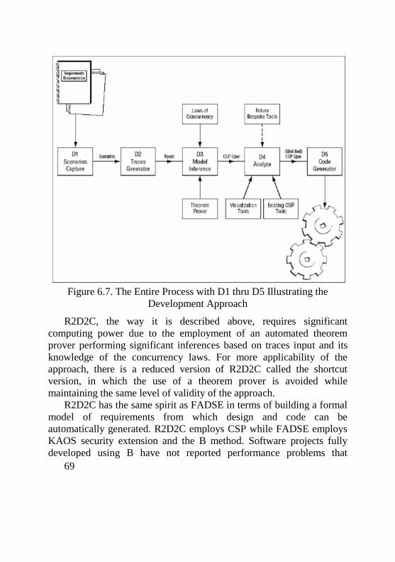
69

Figure 6.7. The Entire Process with D1 thru D5 Illustrating the

Development Approach

R2D2C, the way it is described above, requires significant

computing power due to the employment of an automated theorem

prover performing significant inferences based on traces input and its

knowledge of the concurrency laws. For more applicability of the

approach, there is a reduced version of R2D2C called the shortcut

version, in which the use of a theorem prover is avoided while

maintaining the same level of validity of the approach.

R2D2C has the same spirit as FADSE in terms of building a formal

model of requirements from which design and code can be

automatically generated. R2D2C employs CSP while FADSE employs

KAOS security extension and the B method. Software projects fully

developed using B have not reported performance problems that

70

obstruct the applicability of B to real software due to the level of

maturity and stability of the commercial B tools. R2D2C also considers

transforming the requirements model specified in CSP to B in order to

make use of the code generation capabilities in B tools. Unlike FADSE,

R2D2C captures requirements only in scenarios, which cannot capture

all types of requirements especially security requirements that might

not always be suitable for representation in scenarios.

There are a number of approaches proposed in literature to check

for consistency and compliance between requirements and design or

implementation. This category of approaches is comparable to FADSE

since FADSE allows for the generation of acceptance test cases from

the requirements in order to check for the consistency between the

derived implementation specifications and the requirements model.

The Ontology for Software Specification and Design (OSSD)

approach integrates KAOS and UML to be able to detect errors in

software designs against the original requirements [45]. This is

achieved through integrating UML with the KAOS framework for

elaboration requirements in order to help automate the detection of

inconsistencies in UML designs, which enhances the quality of the

original design and ultimately integrating the multiple views of UML

[45]. OSSD is based on extracting structure, data and relationships from

UML design models; abstracts them into an ontology-based integrated

model; and creates a specification level representation of the original

UML design in a formal, agent-oriented requirements modeling

language, which is KAOS.

A simple set of mappings is used to transform the OSSD model to

an equivalent KAOS model in order to produce requirements

specification that is used as input to an appropriate verification tool in

order to detect inconsistencies between the specifications resulted from

the OSSD approach and the original requirements. The original UML

design is then manually updated based on the results of the verification

processing.

“The transformation from UML to OSSD can be summarized as a

combined lexical and semantic analysis of the UML Model diagrams,

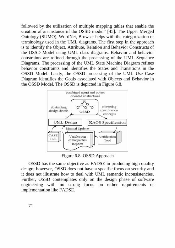
71

followed by the utilization of multiple mapping tables that enable the

creation of an instance of the OSSD model” [45]. The Upper Merged

Ontology (SUMO), WordNet, Browser helps with the categorization of

terminology used in the UML diagrams. The first step in the approach

is to identify the Object, Attribute, Relation and Behavior Constructs of

the OSSD Model using UML class diagrams. Behavior and behavior

constraints are refined through the processing of the UML Sequence

Diagrams. The processing of the UML State Machine Diagram refines

behavior constraints and identifies the States and Transitions in the

OSSD Model. Lastly, the OSSD processing of the UML Use Case

Diagram identifies the Goals associated with Objects and Behavior in

the OSSD Model. The OSSD is depicted in Figure 6.8.

Figure 6.8. OSSD Approach

OSSD has the same objective as FADSE in producing high quality

design; however, OSSD does not have a specific focus on security and

it does not illustrate how to deal with UML semantic inconsistencies.

Further, OSSD contemplates only on the design phase of software

engineering with no strong focus on either requirements or

implementation like FADSE.

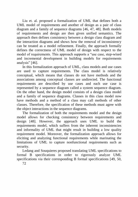
72

Liu et. al. proposed a formalization of UML that defines both a

UML model of requirements and another of design as a pair of class

diagram and a family of sequence diagrams [46, 47, 48]. Both models

of requirements and design are then given unified semantics. The

approach then defines consistency between a design class diagram and

the interaction diagrams and shows how the removal of inconsistency

can be treated as a model refinement. Finally, the approach formally

defines the correctness of UML model of design with respect to the

model of requirements. This approach supports a “use case, step-wised

and incremental development in building models for requirements

analysis” [46].

In this formalization approach of UML, class models and use cases

are used to capture requirements. The class model is relatively

conceptual, which means that classes do not have methods and the

associations among conceptual classes are undirected. The functional

requirements are described by use cases and each use case is

represented by a sequence diagram called a system sequence diagram.

On the other hand, the design model consists of a design class model

and a family of sequence diagrams. Classes in this class model now

have methods and a method of a class may call methods of other

classes. Therefore, the specification of these methods must agree with

the object interactions in the sequence diagrams.

The formalization of both the requirements model and the design

model allows for checking consistency between requirements and

design [48]. However, the approach uses UML to build the

requirements model, which suffers from the inherent inconsistencies

and informality of UML that might result in building a low quality

requirement model. Moreover, the formalization approach allows for

eliciting and analyzing functional requirements while marinating the

limitations of UML to capture nonfunctional requirements such as

security.

Ledang and Souquieres proposed translating UML specifications to

formal B specifications in order to rigorously analyze UML

specifications via their corresponding B formal specifications [49, 50,

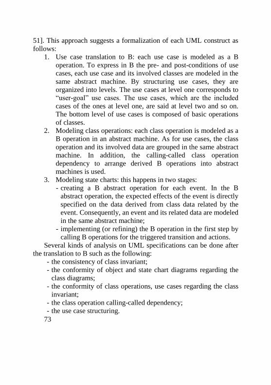
73

51]. This approach suggests a formalization of each UML construct as

follows:

1. Use case translation to B: each use case is modeled as a B

operation. To express in B the pre- and post-conditions of use

cases, each use case and its involved classes are modeled in the

same abstract machine. By structuring use cases, they are

organized into levels. The use cases at level one corresponds to

“user-goal” use cases. The use cases, which are the included

cases of the ones at level one, are said at level two and so on.

The bottom level of use cases is composed of basic operations

of classes.

2. Modeling class operations: each class operation is modeled as a

B operation in an abstract machine. As for use cases, the class

operation and its involved data are grouped in the same abstract

machine. In addition, the calling-called class operation

dependency to arrange derived B operations into abstract

machines is used.

3. Modeling state charts: this happens in two stages:

- creating a B abstract operation for each event. In the B

abstract operation, the expected effects of the event is directly

specified on the data derived from class data related by the

event. Consequently, an event and its related data are modeled

in the same abstract machine;

- implementing (or refining) the B operation in the first step by

calling B operations for the triggered transition and actions.

Several kinds of analysis on UML specifications can be done after

the translation to B such as the following:

- the consistency of class invariant;

- the conformity of object and state chart diagrams regarding the

class diagrams;

- the conformity of class operations, use cases regarding the class

invariant;

- the class operation calling-called dependency;

- the use case structuring.

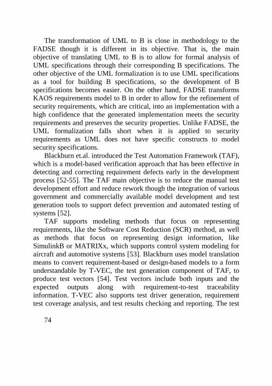
74

The transformation of UML to B is close in methodology to the

FADSE though it is different in its objective. That is, the main

objective of translating UML to B is to allow for formal analysis of

UML specifications through their corresponding B specifications. The

other objective of the UML formalization is to use UML specifications

as a tool for building B specifications, so the development of B

specifications becomes easier. On the other hand, FADSE transforms

KAOS requirements model to B in order to allow for the refinement of

security requirements, which are critical, into an implementation with a

high confidence that the generated implementation meets the security

requirements and preserves the security properties. Unlike FADSE, the

UML formalization falls short when it is applied to security

requirements as UML does not have specific constructs to model

security specifications.

Blackburn et.al. introduced the Test Automation Framework (TAF),

which is a model-based verification approach that has been effective in

detecting and correcting requirement defects early in the development

process [52-55]. The TAF main objective is to reduce the manual test

development effort and reduce rework though the integration of various

government and commercially available model development and test

generation tools to support defect prevention and automated testing of

systems [52].

TAF supports modeling methods that focus on representing

requirements, like the Software Cost Reduction (SCR) method, as well

as methods that focus on representing design information, like

SimulinkB or MATRIXx, which supports control system modeling for

aircraft and automotive systems [53]. Blackburn uses model translation

means to convert requirement-based or design-based models to a form

understandable by T-VEC, the test generation component of TAF, to

produce test vectors [54]. Test vectors include both inputs and the

expected outputs along with requirement-to-test traceability

information. T-VEC also supports test driver generation, requirement

test coverage analysis, and test results checking and reporting. The test

75

drivers are then used to test the implementation functionalities during

the testing phase [55].

Like FADSE, TAF derives test cases from the requirements model

in order to verify the consistency and compliance between requirements

and implementation and to provide sufficient traceability information.

However, TAF is stronger in generating different types of test cases

including unit testing, integration testing and acceptance testing while

FADSE only generates acceptance test cases. This difference is due to

the fact that TAF is a specialized testing framework while FADSE

provides the generation of acceptance test cases as an extra verification

step to ensure that the derived implementation meets the initial set of

security requirements. It might be part of FADSE’ future work to apply

deeper analysis to the KAOS requirements model to generate other type

of test cases.

Rationale

Like many high-assurance applications, there are cost and time

reasons to focus the use of formal methodsto the key aspects of a

system. For large software applications it can be cost-prohibitive to

apply formal methods and many of these large systems have relevant

security concerns. So, a compromise was made and formal methods

were applied to software security aspects of the system in Formal

Analysis and Design for Security Engineering. Further, the

requirements elicitation and specification process is complex and the

additional complexity of formulating these requirements using a formal

method is overwhelming. So, Formal Analysis and Design for Security

Engineering started with Van Lamsweerde’s near-formal, goal-directed

KAOS framework for identifying, elaborating, organizing, analyzing,

and specifying security requirements [4, 2, 4, 3]. KAOS is a proven

semi-formal requirements elaboration framework with an underlying

formal infrastructure based on first-order temporal logic. From this

base, Formal Analysis and Design for Security Engineering transforms

the KAOS requirements specification into B, preserving the security

properties so carefully expressed in KAOS. Then, using the B

76

refinement process, Formal Analysis and Design for Security

Engineering systematically elaborate and refine the security

requirements into a formal B design specification. To accommodate the

fact that KAOS is not fully formal, take the idea of producing a test

case suite based on the requirements model to help increase confidence

through verification. Further, extending KAOS with more formality in a

development platform like B allows for tracing security requirements at

the various steps of development; that is during both design and

implementation.

This section provides an argument for the rationale of the choices of

KAOS and B to employ in Formal Analysis and Design for Security

Engineering. The paradigm shift from the traditional approaches

including semi-formal and formal methods to goalorientation has led

the requirements engineering research community to argue about the

effectiveness and usefulness of the new paradigm. The research effort

in the goal-orientation domain has resulted in the major two

frameworks namely KAOS and i* that represent the current state of the

art in the domain. A number of case studies have been used to

demonstrate the effectiveness of the goal-oriented paradigm and

illustrate its strengths and limitation. The KAOS framework has been

effectively demonstrated on more than 30 industrial projects that report

outstanding success stories [2]. The i* framework has been

demonstrated on a number of case studies, some of them are quite large

systems. However, there is no quantitative analysis that precisely

estimate the gains obtained from applying goal-oriented approaches

over traditional approaches. As Van Lamsweerde and Mylopoulos, et.

al. mentioned that preliminary empirical studies and their own

experience with goal-orientation shows a strong potential in its

application and its extensibility to formal methods [57, 23].

The above mentioned approaches that extend KAOS with extra

formality to fill in the gap between requirements and later phases of

development such as architecture and design show interest of the

research community in the new goal-oriented paradigm. Researchers

who extended KAOS either for architecture or design provided a

77

qualitative argument for their choice of the goal-oriented method. Their

argument has been qualitatively based on the prominent features of

goal-orientation that enables the enhancement of the current

requirements engineering practice. Van Lamsweerde argued for the

strengths of the goal-oriented KAOS framework that makes it suitable

to requirements engineering since it overcomes the limitations of

traditional semi-formal and formal approaches as mentioned above.

There remain still some limitations to the approach in engineering

requirements. The following paragraphs summarize the strengths and

limitations of the KAOS framework. The following key points about

goal orientation justify the choice of the goal-oriented KAOS

framework for requirements analysis in Formal Analysis and Design for

Security Engineering [57].

Goal-oriented modeling and specification takes a wider system

engineering perspective; goals are prescriptive assertions that should

hold in the system made of the software-to-be and its environment;

domain properties and expectations about the environment are

explicitly captured during the requirements elaboration process, in

addition to the usual software requirements specifications.

1. Operational requirements are derived incrementally from the

higher-level system goals they “implement”.

1. Goals provide the rationale for the requirements that

operationalize them and, in addition, a correctness criterion for

requirements completeness and pertinence [58].

2. Obstacle analysis helps producing much more robust systems

by systematically generating (a) potential ways in which the

system might fail to meet its goals and (b) alternative ways of

resolving such problems early enough during the requirements

elaboration and negotiation phase.

3. Alternative system proposals are explored through alternative

goal refinements, responsibility assignments, obstacle

resolutions and conflict resolutions.

4. The goal refinement structure provides a rich way of structuring

and documenting the entire requirements document.

78

5. Different levels of formality could be offered by the framework

allowing one to combine different levels of expression and

reasoning: semi-formal for modeling and structuring,

qualitative for selection among alternatives, and formal, when

needed, for more accurate reasoning.

6. Goal formalization allows requirements engineering-specific

types of analysis to be carried out, like:

- guiding the goal refinement process and the systematic

identification of objects and agents [7, 59];

- checking the correctness of goal refinements and detecting

missing goals and implicit assumptions [11];

- guiding the identification of obstacles and their resolutions

[59];

- guiding the identification of conflicts and their resolutions

[2];

- guiding the identification and specification of operational

requirements that satisfy the goals [8, 60].

Van Lamsweerde argument of the goal-orientation characteristics

that offer better handling of requirements analysis is supported by

Mylopoulos, et. al. argument in [23]. Mylopoulos, et. al. argued that the

adoption of the goal-oriented mindset is very important during

requirements analysis because it deals with non-functional requirements

and relates them to functional ones [23]. Further, goal-oriented analysis

focuses on the description and evaluation of alternatives and their

relationship to the organizational objectives behind a software

development project. Many of the requirements engineering research

community have argued that capturing these interdependencies between

organizational objectives and the detailed software requirements can

facilitate the tracing of the origins of requirements and can help make

the requirements process more thorough, complete, and consistent [23].

Mylopoulos, et. al. have strengthened their argument in favor of the

goal-oriented paradigm by preliminary empirical studies showing that

goal-oriented analysis can indeed lead to a more complete requirements

definition than OOA techniques. Further, the authors’ own experiences

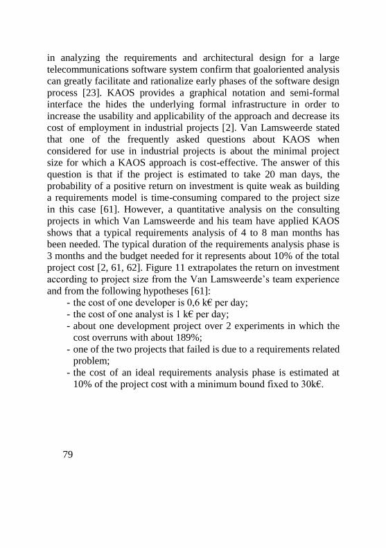
79

in analyzing the requirements and architectural design for a large

telecommunications software system confirm that goaloriented analysis

can greatly facilitate and rationalize early phases of the software design

process [23]. KAOS provides a graphical notation and semi-formal

interface the hides the underlying formal infrastructure in order to

increase the usability and applicability of the approach and decrease its

cost of employment in industrial projects [2]. Van Lamsweerde stated

that one of the frequently asked questions about KAOS when

considered for use in industrial projects is about the minimal project

size for which a KAOS approach is cost-effective. The answer of this

question is that if the project is estimated to take 20 man days, the

probability of a positive return on investment is quite weak as building

a requirements model is time-consuming compared to the project size

in this case [61]. However, a quantitative analysis on the consulting

projects in which Van Lamsweerde and his team have applied KAOS

shows that a typical requirements analysis of 4 to 8 man months has

been needed. The typical duration of the requirements analysis phase is

3 months and the budget needed for it represents about 10% of the total

project cost [2, 61, 62]. Figure 11 extrapolates the return on investment

according to project size from the Van Lamsweerde’s team experience

and from the following hypotheses [61]:

- the cost of one developer is 0,6 k€ per day;

- the cost of one analyst is 1 k€ per day;

- about one development project over 2 experiments in which the

cost overruns with about 189%;

- one of the two projects that failed is due to a requirements related

problem;

- the cost of an ideal requirements analysis phase is estimated at

10% of the project cost with a minimum bound fixed to 30k€.

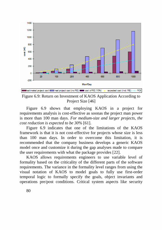
80

Figure 6.9: Return on Investment of KAOS Application According to

Project Size [46]

Figure 6.9 shows that employing KAOS in a project for

requirements analysis is cost-effective as soonas the project man power

is more than 100 man days. For medium-size and larger projects, the

cost reduction is expected to be 30% [61].

Figure 6.9 indicates that one of the limitations of the KAOS

framework is that it is not cost-effective for projects whose size is less

than 100 man days. In order to overcome this limitation, it is

recommended that the company business develops a generic KAOS

model once and customize it during the gap analyses made to compare

the user requirements with what the package provides [22].

KAOS allows requirements engineers to use variable level of

formality based on the criticality of the different parts of the software

requirements. The variance in the formality level ranges from using the

visual notation of KAOS to model goals to fully use first-order

temporal logic to formally specify the goals, object invariants and

operations pre/post conditions. Critical system aspects like security

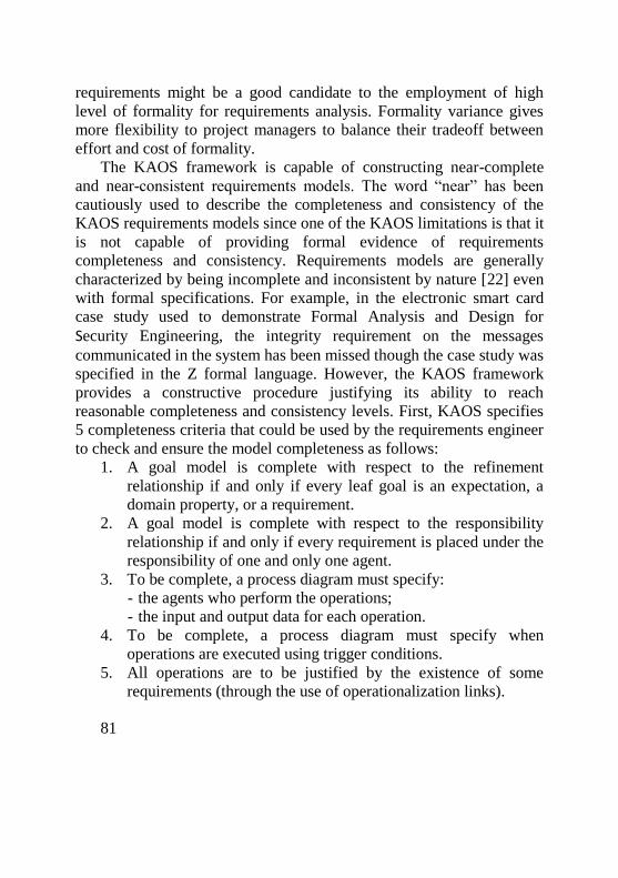
81

requirements might be a good candidate to the employment of high

level of formality for requirements analysis. Formality variance gives

more flexibility to project managers to balance their tradeoff between

effort and cost of formality.

The KAOS framework is capable of constructing near-complete

and near-consistent requirements models. The word “near” has been

cautiously used to describe the completeness and consistency of the

KAOS requirements models since one of the KAOS limitations is that it

is not capable of providing formal evidence of requirements

completeness and consistency. Requirements models are generally

characterized by being incomplete and inconsistent by nature [22] even

with formal specifications. For example, in the electronic smart card

case study used to demonstrate Formal Analysis and Design for

Security Engineering, the integrity requirement on the messages

communicated in the system has been missed though the case study was

specified in the Z formal language. However, the KAOS framework

provides a constructive procedure justifying its ability to reach

reasonable completeness and consistency levels. First, KAOS specifies

5 completeness criteria that could be used by the requirements engineer

to check and ensure the model completeness as follows:

1. A goal model is complete with respect to the refinement

relationship if and only if every leaf goal is an expectation, a

domain property, or a requirement.

2. A goal model is complete with respect to the responsibility

relationship if and only if every requirement is placed under the

responsibility of one and only one agent.

3. To be complete, a process diagram must specify:

- the agents who perform the operations;

- the input and output data for each operation.

4. To be complete, a process diagram must specify when

operations are executed using trigger conditions.

5. All operations are to be justified by the existence of some

requirements (through the use of operationalization links).

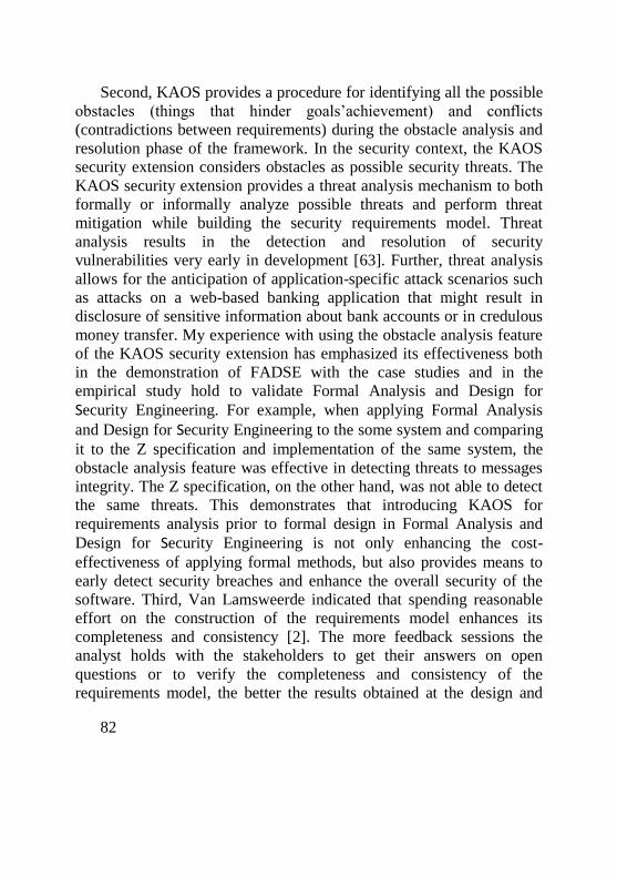
82

Second, KAOS provides a procedure for identifying all the possible

obstacles (things that hinder goals’achievement) and conflicts

(contradictions between requirements) during the obstacle analysis and

resolution phase of the framework. In the security context, the KAOS

security extension considers obstacles as possible security threats. The

KAOS security extension provides a threat analysis mechanism to both

formally or informally analyze possible threats and perform threat

mitigation while building the security requirements model. Threat

analysis results in the detection and resolution of security

vulnerabilities very early in development [63]. Further, threat analysis

allows for the anticipation of application-specific attack scenarios such

as attacks on a web-based banking application that might result in

disclosure of sensitive information about bank accounts or in credulous

money transfer. My experience with using the obstacle analysis feature

of the KAOS security extension has emphasized its effectiveness both

in the demonstration of FADSE with the case studies and in the

empirical study hold to validate Formal Analysis and Design for

Security Engineering. For example, when applying Formal Analysis

and Design for Security Engineering to the some system and comparing

it to the Z specification and implementation of the same system, the

obstacle analysis feature was effective in detecting threats to messages

integrity. The Z specification, on the other hand, was not able to detect

the same threats. This demonstrates that introducing KAOS for

requirements analysis prior to formal design in Formal Analysis and

Design for Security Engineering is not only enhancing the cost-

effectiveness of applying formal methods, but also provides means to

early detect security breaches and enhance the overall security of the

software. Third, Van Lamsweerde indicated that spending reasonable

effort on the construction of the requirements model enhances its

completeness and consistency [2]. The more feedback sessions the

analyst holds with the stakeholders to get their answers on open

questions or to verify the completeness and consistency of the

requirements model, the better the results obtained at the design and

83

implementation phases. The KAOS goal graph is a structure that could

be communicated with the stakeholders who often have no technical

background. Providing a structure that could be understood and

communicated to stakeholders allows requirements engineers to get

more thorough feedback from stakeholders to enhance the

completeness and consistency of the requirements model.

The choice of B as a formal development platform for elaborating

security design specifications assists in preserving security properties of

requirements when design specifications are being derived. B has the

notion of model refinement that allows for building a detailed model of

design from an abstract model of requirements while preserving the

security properties of the requirements model. The refinement

mechanism in B provides a means for documenting design decisions

and building forward traceability links from requirements to design.

Hence, the links between artifacts are clear enough to provide

traceability information that serves software maintenance activities,

which might be performed after the software is fully developed. The

use of a software model that stores design decisions and traceability

links significantly improves the accuracy and completeness of impact

analysis that is concerned with identifying the impact of a given change

on the software product [65]. Moreover, B is based on set mathematics

with the ability to use standard first-order predicate logic facilitating the

integration with the KAOS security requirements model that is based

on first-order temporal logic. Further, B is a mature formal method that

has been successfully employed in industrial projects for long time. The

availability of good tool support for the B development platform

strengths the practicality and applicability of Formal Analysis and

Design for Security Engineering.

Employing formal methods in Formal Analysis and Design for

Security Engineering provides a reasonable approach to the challenge

of developing secure software products with formal evidence of

correctness [64]. Recognizing that formal methods reduce security risks

but entails more cost, it is possible to justify this cost by applying

84

Formal Analysis and Design for Security Engineering only to security,

which is a critical aspect of the system. Further, software systems that

are evaluated for security at the Common Criteria (CC) EAL

(Evaluation Assurance Level) 5, 6 and 7 need formal evidence assuring

the security of the software. This makes software products developed

using Formal Analysis and Design for Security Engineering securely

compliant with CC higher levels.

Formal Analysis and Design for Security Engineering is a step

towards the development of highly secure software. In a nutshell,

Formal Analysis and Design for Security Engineering is a

requirements-driven software engineering approach that derives design

specifications from a set of security requirements modeled using KAOS

security extension framework. The approach provides a secure software

engineering methodology that effectively integrates KAOS security

extension,which is characterized by the ability to formally build a

complete, consistent and clear requirements model with the B method,

which provides formal guarantees for the correctness of the system

development. This research showed that KAOS is promising in that it

could be extended with an extra step of formality in order to fully

implement security requirements while preserving the security

properties specified in therequirements model. Moreover, extending

KAOS with more formality in a development framework like B allows

for tracing requirements at the various steps of development; that is,

during both design and implementation.

Formal Analysis and Design for Security Engineering starts with a

set of security requirements that are being elaborated with the KAOS

security extension to build a goal graph for the security requirements

and derive the operations that achieve the goals. Formal Analysis and

Design for Security Engineering makes use of the analytical capabilities

provided with the goal graph to achieve two objectives. The first

objective is to transform the KAOS operations derived to achieve the

goals to B using means of the transformation scheme described below

in order to construct an abstract B model that describes the initial

85

system state and its expected security behavior. The initial B machine is

further refined using the B refinement mechanism to add more details

while building the security design specifications. The second objective

is to derive acceptance test cases from the goal graph outlining the

different scenarios of security behavior that should be met by the

derived B design and implementation specifications. This means that

the goal graph is used to derive the initial abstract B model that will be

further refined for design and implementation and to derive means to

verify that the derived design and implementation meet the security

requirements objectives through the acceptance test cases. The

completeness and consistency of the derived implementation

specifications are a function of the successful verification of the

implementation against the acceptance test cases. The extra verification

step that Formal Analysis and Design for Security Engineering provides

through the derivation of test cases allows for detecting inconsistencies

that might have been in the requirements model or in the process of

design and implementation derivation. The test cases guarantee the

same level of completeness and consistency of the requirements model

since they are derived using a depth first search algorithm. The

algorithm traverses the goal graph to generate sequence of calls to

operations in the correct order that matches the semantics of the high

level goals in the goal graph. The test cases provide means to detect

possible security hazards that might result from inconsistencies either in

the requirements model or in design. Formal Analysis and Design for

Security Engineering is illustrated in Figure 6.10.

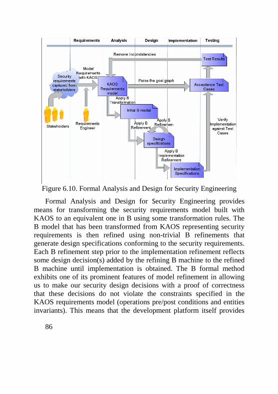
86

Figure 6.10. Formal Analysis and Design for Security Engineering

Formal Analysis and Design for Security Engineering provides

means for transforming the security requirements model built with

KAOS to an equivalent one in B using some transformation rules. The

B model that has been transformed from KAOS representing security

requirements is then refined using non-trivial B refinements that

generate design specifications conforming to the security requirements.

Each B refinement step prior to the implementation refinement reflects

some design decision(s) added by the refining B machine to the refined

B machine until implementation is obtained. The B formal method

exhibits one of its prominent features of model refinement in allowing

us to make our security design decisions with a proof of correctness

that these decisions do not violate the constraints specified in the

KAOS requirements model (operations pre/post conditions and entities

invariants). This means that the development platform itself provides

87

constructs to reduce risks of introducing errors in development. After

applying a number of refinement steps to the initial B model, an

implementation refinement step, which is a special refinement step in B

is applied.

Formal Analysis and Design for Security Engineering allows for

deriving one artifact, which is design from another artifact, which is a

requirements model using formal representation in B. The refinement

mechanism in B provides means for documenting design decisions and

building forward traceability links from requirements to design. Hence,

the links between artifacts are clear enough to provide traceability

information that serves the purposes of software maintenance activities

that might be performed after the software is fully developed. The use

of a software model that stores design decisions and traceability links

significantly improves the accuracy and completeness of impact

analysis that is concerned with identifying the impact of a given change

on the software product [65].

The derived implementation specifications are then verified against

the test cases that have been drawn from the KAOS requirements

model. Our results have shown that the major two sources for problems

encountered in implementation are inconsistencies either in the

requirements model or in the design decisions made during the B

refinement steps. The derived test cases are capable of detecting some

inconsistencies in both the requirements model and design. Further, the

ratio between the numbers of successful test cases and failed test cases

can be used as exit criteria for security assurance and this is evidenced

in the Common Criteria Evaluation Assessment Levels (EAL) 5, 6 and

7. The feedback loop established from the test cases results to the

requirements model as indicated in the Figure 6.11 allows for detecting

possible security hazards a priori to deploying the software system into

production at which time “real” security threats might be encountered.

Formal Analysis and Design for Security Engineering is

characterized with some features that make it more attractive to apply

over other similar formal approaches. These features are either inherent

88

from the underlying approaches employed in Formal Analysis and

Design for Security Engineering, namely KAOS and B or new in

Formal Analysis and Design for Security Engineering. It addresses

security-specific elements of software to bridge the gap between

security requirements and their realization in design and

implementation. Up to our knowledge, Formal Analysis and Design for

Security Engineering is the first approach to address the gap between

requirements and design for security requirements specifically. Formal

Analysis and Design for Security Engineering is promising in being

ready for wide applicability thanks to the strong tool support provided

by the underlying technologies of KAOS and B. KAOS has a

commercial tool called Objectiver [61] that has been commercially used

in a number of successful industrial projects. B has been in the

industrial market for a while with its most two famous commercial

products namely AtelierB and the B-Toolkit [66, 67]. The availability

of strong tool support strengths the practicality and applicability of

Formal Analysis and Design for Security Engineering.

Formal Analysis and Design for Security Engineering takes KAOS

with a further step of formality to derive design and implementation

through transforming the KAOS requirements model to B. The initial B

model obtained from the automatic transformation enforce the same

security constraints specified in the KAOS requirements model

modeled in the form of preconditions of the B operations that model the

KAOS operations and the B machine invariants that model the KAOS

entities invariants. The definition of these constraints in the initial B

model forces the preservation of these constraints at the later B

refinements steps that add more details to the initial B model to commit

design decisions. The proof obligation facility provided with B method

and that could be automatically generated using one of the commercial

B tools allows software security developers to discharge the generated

proof obligations to ensure correctness of development. Discharging the

proof obligations formally proves that a refinement step in B does not

violate the constraints of the more abstract B model being refined.

89

Formal Analysis and Design for Security Engineering provides an extra

verification step to show the maintenance of security properties

specified in the requirements model in the derived implementation

specifications. This is achieved when deriving a set of test cases that are

generated from traversing the KAOS goal graph. The test cases provide

security developers with means to assure a reasonable level of

completeness and consistency of their implementation with respect to

the requirements model. Finally, one of the key merits of employing

formal methods in Formal Analysis and Design for Security

Engineering is the availability of sufficient traceability information that

links requirements to design decisions giving better opportunities for

more accurate and less vulnerable handling of changes to security

specifications.

Transforming KAOS to B

The Knowledge Acquisition for autOmated Specifications

requirements model is represented in the form of a directed-acyclic

graph rooted at the very high level goal of the system and structured in

multiple levels. Goals at each level refine the goals at the higher level.

An example of a goal graph for the security requirements of the spy

network system is illustrated as an example in Figure 6.12. The

diamond shapes represent security goals while the rectangles with

circular corners represent agents responsible to achieve leaf goal

requirements.

The whole system is represented either as a single abstract B

machine or multiple abstract B machines related to each other based on

the size of the system. Each KAOS entity (passive object) is

represented as a B machine included or seen by the system machine(s)

and encapsulating its KAOS attributes and operations manipulating the

attributes as follows:

- the entity attributes are variables in the equivalent B machine

representing the state of the object;

90

- the B machine invariant is composed of the types of the

attributes’ variables (might be primitive types or types from other

KAOS entities) and the domain invariant of the KAOS object

presented in first-order predicate logic;

- each B machine representing an entity includes a set representing

all its instances because B is not an object oriented language,

rather it is instance-based. Entity attributes are represented as

relations between the set of instances and the attribute types. This

representation of the instances and their attributes allows for the

use of the set arithmetic capabilities of B.

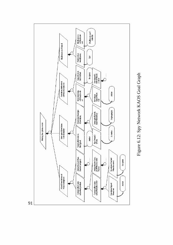
91

Fig

ure

6.1

2:

Spy N

etw

ork

KA

OS

Goal

Gra

ph

92

Each KAOS operation is represented as a B operation in the system

machine and uses the KAOS entities either as parameters or return

values. KAOS operations pre/post and trigger conditions are treated in

the transformation as follows:

- pre-condition are directly mapped to a B precondition for the B

operation since both KAOS and B preconditions are written in

first order-predicate logic;

- post-condition has no equivalent construct in B. The operation

specification and refinement should be responsible for enforcing

the KAOS operation post-condition. This means that the post

condition of the KAOS operation should be used in the operation

specification, which is not part of the transformation. The

transformation is only limited to building the requirements model

that represent the KAOS model. It is the responsibility of the

designer to fill in the body of each operation while taking into

consideration the KAOS operation post-condition;

- trigger-condition has no direct mapping to the trigger condition

in B. The trigger condition in KAOS is used to model the

sequence of operation calls and the conditions that would lead to

calling the operation. The trigger condition could be forced by

the agents who are controlling the system runtime execution.

Further, it is the responsibility of the agent calling the operations

to prepare all the operations trigger conditions in a true state for

the operation to be called.

Agents (active objects) are not directly transformed to KAOS since

they are responsible for the runtime behavior of the system. Agents’

behavior is modeled through the transformed KAOS operations. The

acceptance test cases derived from the KAOS goal graph simulate the

agent behavior in executing the KAOS operations that realized the

requirements goals. KAOS goals are not transformed to B since their

semantics is encapsulated in the KAOS operations that realize the leaf

goals. The achievement of leaf goals through KAOS operations implies

the achievement of the higher-level goals through the KAOS AND/OR

refinement process. The KAOS goals and their sequence of refinement

93

are used to derive the acceptance test cases that are used to increase our

confidence in the derived implementation specifications to be

consistent and complete with respect to the requirements model.

Further, KAOS goals in the goal graph are used to provide links for

requirement traceability. Design decisions can be easily linked to

higher-level goals using the goal graph structure that indicates which

goals are realized by which operation (s). Traceability information

plays a crucial role in accurately specifying the impact of applying a

change to security specifications. KAOS domain properties are

captured in B as invariants to the B machines that model the KAOS

objects and as pre/post conditions to the operations that model KAOS

operations. Objects invariants as well as operations pre conditions are

preserved during the B refinement steps meaning that the domain

properties are maintained throughout the software development

lifecycle using the proposed approach. KAOS scenarios are not

considered in the transformation scheme since scenarios are used as a

vehicle security requirements engineer uses to assure the customer that

all the security requirements are well understood and captured. The

primary objective of the transformation from KAOS to B is to develop

security design specifications that need to detail the implementation

plan of the security requirements rather than focusing, as in the

requirements analysis phase, on providing evidence that the customer

can understand such as scenarios.

The rules of the transformation scheme from KAOS to B are

summarized in Table 6.1.

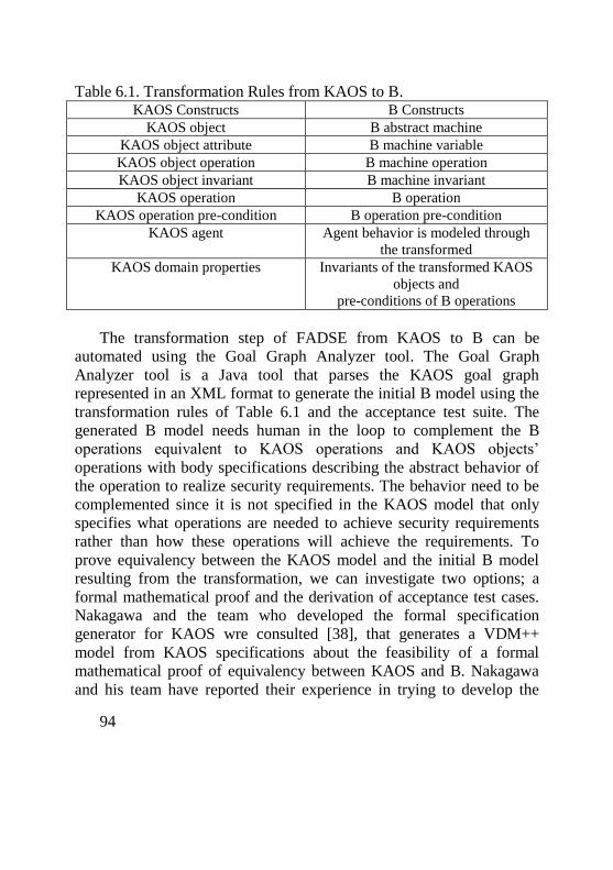
94

Table 6.1. Transformation Rules from KAOS to B. KAOS Constructs B Constructs

KAOS object B abstract machine

KAOS object attribute B machine variable

KAOS object operation B machine operation

KAOS object invariant B machine invariant

KAOS operation B operation

KAOS operation pre-condition B operation pre-condition

KAOS agent Agent behavior is modeled through

the transformed

KAOS domain properties

Invariants of the transformed KAOS

objects and

pre-conditions of B operations

The transformation step of FADSE from KAOS to B can be

automated using the Goal Graph Analyzer tool. The Goal Graph

Analyzer tool is a Java tool that parses the KAOS goal graph

represented in an XML format to generate the initial B model using the

transformation rules of Table 6.1 and the acceptance test suite. The

generated B model needs human in the loop to complement the B

operations equivalent to KAOS operations and KAOS objects’

operations with body specifications describing the abstract behavior of

the operation to realize security requirements. The behavior need to be

complemented since it is not specified in the KAOS model that only

specifies what operations are needed to achieve security requirements

rather than how these operations will achieve the requirements. To

prove equivalency between the KAOS model and the initial B model

resulting from the transformation, we can investigate two options; a

formal mathematical proof and the derivation of acceptance test cases.

Nakagawa and the team who developed the formal specification

generator for KAOS wre consulted [38], that generates a VDM++

model from KAOS specifications about the feasibility of a formal

mathematical proof of equivalency between KAOS and B. Nakagawa

and his team have reported their experience in trying to develop the

95

mathematical proof as infeasible since the KAOS model is a

requirements model involving undefined parameters making the proof

very hard to develop within a reasonable timeframe. Moreover, the

automation of the transformation reduces its error-proneness since

automation rigidly applies the transformation rules. Further, the fact

that both KAOS and B employ firstorder predicate logic to express

system constraints and conditions facilitates the transformation and

reduces the probability of an equivalency gap between the KAOS

model and the transformed B model. The acceptance test case option

has been more feasible to realize any errors that might result from the

transformation scheme. The KAOS goal graph is used to derive the

initial abstract B model that will be further refined for design and

implementation and to derive means to verify that the derived design

and implementation meet the security requirements objectives through

the acceptance test cases. Our results have shown that the major two

sources of problems encountered in implementation are inconsistencies

either in the requirements model or in the design decisions made during

the B refinement steps, but not in the transformation rules.

Derivation of Acceptance Test Cases

Formal Analysis and Design for Security Engineering provides an

extra verification step to show the maintenance of security properties

specified in the requirements model in the derived implementation

specifications. FADSE derives a suite of acceptance test cases through

traversing the KAOS goal graph. The test cases provide security

developers with means to assure a reasonable level of completeness and

consistency of their implementation with respect to the requirements

model. The KAOS goal graph is rooted at the very high level goal of

the system while leaf goals at the very bottom of the goal graph

represent requirements. Each requirement is realized with an operation

performed by an agent in the software-to-be. This means that the

sequence of operations that need to be performed in order to execute a

goal at a middle level of the goal graph can be identified using a depth

first search (DFS) algorithm for the subgraph rooted at this goal. A DFS

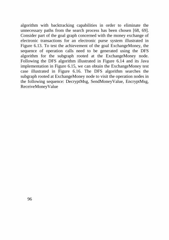
96

algorithm with backtracking capabilities in order to eliminate the

unnecessary paths from the search process has been chosen [68, 69].

Consider part of the goal graph concerned with the money exchange of

electronic transactions for an electronic purse system illustrated in

Figure 6.13. To test the achievement of the goal ExchangeMoney, the

sequence of operation calls need to be generated using the DFS

algorithm for the subgraph rooted at the ExchangeMoney node.

Following the DFS algorithm illustrated in Figure 6.14 and its Java

implementation in Figure 6.15, we can obtain the ExchangeMoney test

case illustrated in Figure 6.16. The DFS algorithm searches the

subgraph rooted at ExchangeMoney node to visit the operation nodes in

the following sequence: DecryptMsg, SendMoneyValue, EncryptMsg,

ReceiveMoneyValue

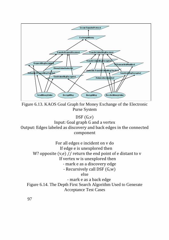
97

Figure 6.13. KAOS Goal Graph for Money Exchange of the Electronic

Purse System

DSF (G,v) Input: Goal graph G and a vertex

Output: Edges labeled as discovery and back edges in the connected component

For all edges e incident on v do If edge e is unexplored then

W? opposite (v,e) // return the end point of e distant to v If vertex w is unexplored then - mark e as a discovery edge - Recursively call DSF (G,w)

else - mark e as a back edge

Figure 6.14. The Depth First Search Algorithm Used to Generate

Acceptance Test Cases

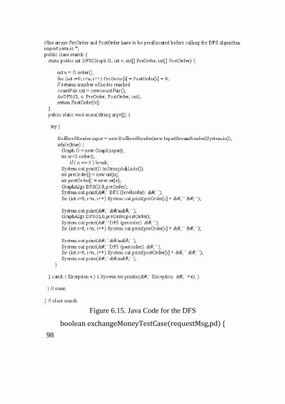
98

Figure 6.15. Java Code for the DFS

boolean exchangeMoneyTestCase(requestMsg,pd) {

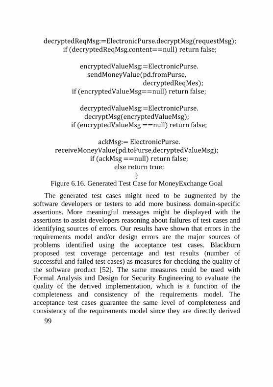
99

decryptedReqMsg:=ElectronicPurse.decryptMsg(requestMsg); if (decryptedReqMsg.content==null) return false;

encryptedValueMsg:=ElectronicPurse.

sendMoneyValue(pd.fromPurse, decryptedReqMes);

if (encryptedValueMsg==null) return false;

decryptedValueMsg:=ElectronicPurse. decryptMsg(encryptedValueMsg);

if (encryptedValueMsg ==null) return false;

ackMsg:= ElectronicPurse. receiveMoneyValue(pd.toPurse,decryptedValueMsg);

if (ackMsg ==null) return false; else return true;

} Figure 6.16. Generated Test Case for MoneyExchange Goal

The generated test cases might need to be augmented by the

software developers or testers to add more business domain-specific

assertions. More meaningful messages might be displayed with the

assertions to assist developers reasoning about failures of test cases and

identifying sources of errors. Our results have shown that errors in the

requirements model and/or design errors are the major sources of

problems identified using the acceptance test cases. Blackburn

proposed test coverage percentage and test results (number of

successful and failed test cases) as measures for checking the quality of

the software product [52]. The same measures could be used with

Formal Analysis and Design for Security Engineering to evaluate the

quality of the derived implementation, which is a function of the

completeness and consistency of the requirements model. The

acceptance test cases guarantee the same level of completeness and

consistency of the requirements model since they are directly derived

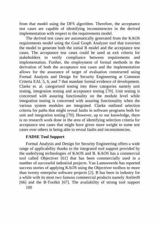
100

from that model using the DFS algorithm. Therefore, the acceptance

test cases are capable of identifying inconsistencies in the derived

implementation with respect to the requirements model.

The derived test cases are automatically generated from the KAOS

requirements model using the Goal Graph Analyzer tool that traverses

the model to generate both the initial B model and the acceptance test

cases. The acceptance test cases could be used as exit criteria for

stakeholders to verify compliance between requirements and

implementation. Further, the employment of formal methods in the

derivation of both the acceptance test cases and the implementation

allows for the assurance of target of evaluation constructed using

Formal Analysis and Design for Security Engineering at Common

Criteria EAL 5, 6, and 7 that mandate formal evidence of development.

Clarke et. al. categorized testing into three categories namely unit

testing, integration testing and acceptance testing [70]. Unit testing is

concerned with assuring functionality on the module level while

integration testing is concerned with assuring functionality when the

various system modules are integrated. Clarke outlined selection

criteria for paths that might reveal faults in software programs both for

unit and integration testing [70]. However, up to our knowledge, there

is no research work done in the area of identifying selection criteria for

acceptance test cases that might have given more weight to some test

cases over others in being able to reveal faults and inconsistencies.

FADSE Tool Support

Formal Analysis and Design for Security Engineering offers a wide

range of applicability thanks to the integrated tool support provided by

the underlying technologies of KAOS and B. KAOS has a commercial

tool called Objectiver [61] that has been commercially used in a

number of successful industrial projects. Van Lamsweerde has reported

success stories of applying KAOS using the Objectiver toolbox to more

than twenty enterprise software projects [2]. B has been in industry for

a while with its most two famous commercial products namely AtelierB

[66] and the B-Toolkit [67]. The availability of strong tool support

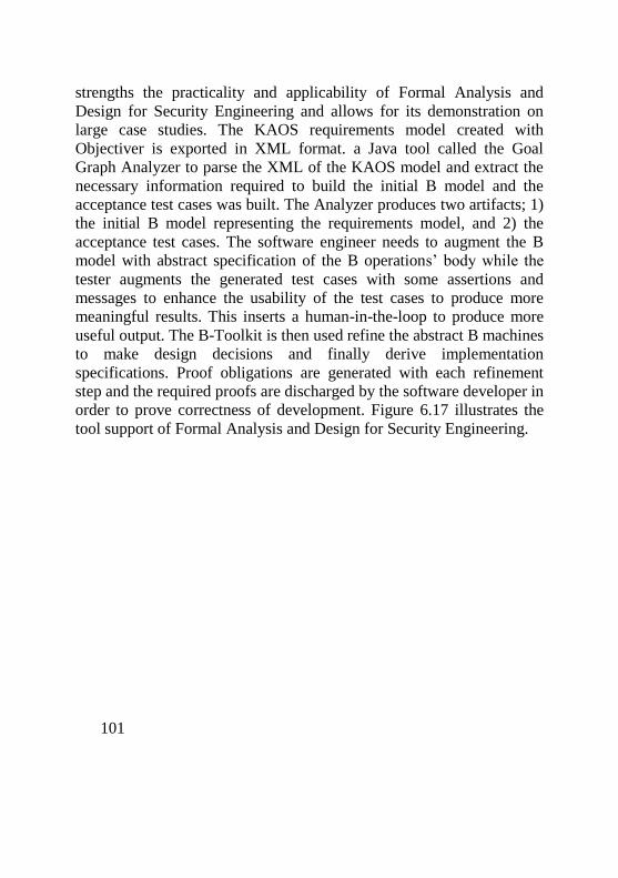
101

strengths the practicality and applicability of Formal Analysis and

Design for Security Engineering and allows for its demonstration on

large case studies. The KAOS requirements model created with

Objectiver is exported in XML format. a Java tool called the Goal

Graph Analyzer to parse the XML of the KAOS model and extract the

necessary information required to build the initial B model and the

acceptance test cases was built. The Analyzer produces two artifacts; 1)

the initial B model representing the requirements model, and 2) the

acceptance test cases. The software engineer needs to augment the B

model with abstract specification of the B operations’ body while the

tester augments the generated test cases with some assertions and

messages to enhance the usability of the test cases to produce more

meaningful results. This inserts a human-in-the-loop to produce more

useful output. The B-Toolkit is then used refine the abstract B machines

to make design decisions and finally derive implementation

specifications. Proof obligations are generated with each refinement

step and the required proofs are discharged by the software developer in

order to prove correctness of development. Figure 6.17 illustrates the

tool support of Formal Analysis and Design for Security Engineering.

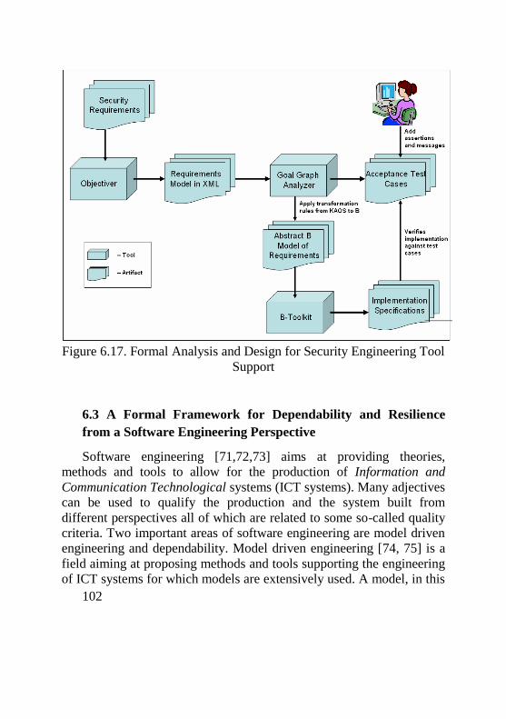
102

Figure 6.17. Formal Analysis and Design for Security Engineering Tool

Support

6.3 A Formal Framework for Dependability and Resilience

from a Software Engineering Perspective

Software engineering [71,72,73] aims at providing theories,

methods and tools to allow for the production of Information and

Communication Technological systems (ICT systems). Many adjectives

can be used to qualify the production and the system built from

different perspectives all of which are related to some so-called quality

criteria. Two important areas of software engineering are model driven

engineering and dependability. Model driven engineering [74, 75] is a

field aiming at proposing methods and tools supporting the engineering

of ICT systems for which models are extensively used. A model, in this

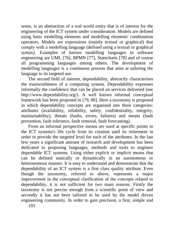
103

sense, is an abstraction of a real world entity that is of interest for the

engineering of the ICT system under consideration. Models are defined

using basic modelling elements and modelling elements' combination

operators. Models are expressions (mainly textual or graphical) that

comply with a modelling language (defined using a textual or graphical

syntax). Examples of known modelling languages in software

engineering are UML [76], BPMN [77], Statecharts [78] and of course

all programming languages among others. The development of

modelling languages is a continuous process that aims at tailoring the

language to its targeted use.

The second field of interest, dependability, abstractly characterises

the trustworthiness of a computing system. Dependability expresses

informally the confidence that can be placed on services delivered (see

http://www.dependability.org/). A well known informal conceptual

framework has been proposed in [79, 80]. Here a taxonomy is proposed

in which dependability concepts are organised into three categories:

attributes (availability, reliability, safety, confidentiality, integrity,

maintainability), threats (faults, errors, failures) and means (fault

prevention, fault tolerance, fault removal, fault forecasting).

From an informal perspective means are used at specific points in

the ICT systems's life cycle from its creation until its retirement in

order to provide the targeted level for each of the attributes. In the last

few years a significant amount of research and development has been

dedicated to proposing languages, methods and tools to engineer

dependable ICT systems. Using either explicit or implicit means that

can be defined statically or dynamically in an autonomous or

heteronomous manner. It is easy to understand and demonstrate that the

dependability of an ICT system is a first class quality attribute. Even

though the taxonomy, referred to above, represents a major

improvement in the conceptual clarification of the concepts related to

dependability, it is not sufficient for two main reasons. Firstly the

taxonomy is not precise enough from a scientific point of view and

secondly it has not been tailored to be used by the model driven

engineering community. In order to gain precision, a first, simple and

104

commonly agreed upon approach is to provide a mathematical

definition. To be compatible with the model driven engineering

paradigm, this definition should be given using meta-modelling

techniques.

Resilience in ICT systems, introduced around the seventies [81] has

been most intensively used within the research community in the very

few last years. By reviewing the important references we can notice

that the word resilience, is used with a variety of definitions and at

different levels [82, 83, 84]. With the same intention described

previously, it is in the interest of ICT systems engineering community

to derive a precise definition of resilience that can be also integrated

into modelling languages.

With respect to the mathematical definition of concepts that are

useful to understand dependability and resilience, we could use many

fields (sets theory, mathematical logic, category theory, mathematical

statistics and geometry among others) at different abstraction levels.

Field selection should depend on the targeted exploitation of the

formalisation. In this article, it is proposed to use algebra (mainly

elementary algebra and basis of general algebra focusing on set theory

and functions) since it is one of the mostly used mathematical fields by

ICT systems engineers and scientists. Its concepts are easily mapped to

the ones that exist in technological fields like programming languages

and data bases. In addition, the concepts correspond to the terminology

used in the natural language of document production throughout the

ICT systems procurement life cycle (such as requirement document,

verification and validation plans). Last but not least, the abstraction

level chosen for the framework proposed in this article makes this

choice appropriate. The intention is also that the framework should

allow for being refined such that more detailed definitions of its

concepts using different mathematical structures may be introduced in a

consistent way with the framework. This should be considered at the

105

modelling language definition level. As an example, the dependability

and resilience of a system might be dependent upon the metrics that can

be defined based on probabilities, statistics, logical systems, model

checking or test results. Thus these metrics should of course be present

in the language used to model the dependable or resilient system.

In order to allow for the exploitation of the framework proposed in

this article (called DREF for Dependability and Resilience Engineering

Framework) in the modelling language definition, some integration

techniques must be provided. To this aim and following the model

driven engineering (MDE) perspective, a meta-model for the DREF

framework was proposed to define. Further, the process for engineering

new domain specific modelling languages (DSL) using a model driven

engineering approach is presented. In this process, let us define how to

exploit the DREF meta-model when introducing a new DSL. As

proposed in this article, this can be done either by extending the

existing DSL to integrate dependability and resilience support or upon

creating the new DSLs.

In the following discussion, the formal conceptual framework for

dependability and resilience is provided along with some basic

illustrations. Then an approach for integrating the proposed framework

into a modelling language definition is proposed and illustrated through

a simple case study. A critical analysis and perspective section is then

proposed to help understand the focus of this work.

Definition of a formal conceptual framework for dependability

and resilience

In this section let us introduce all the concepts needed to define

resilience. The main goal of these sections is to provide a precise

mathematical set of definitions for all notions necessary to address

resiliency.

106

Entities, Properties and satisfiability

The two first basic sets of the proposed conceptual framework

(named DREF ) are the sets of entities and properties. Entities are

anything that is of interest to be considered. It might be a program, a

database, a person, a hardware element, a development process, a

requirement document, et cetera. Properties are the basic concepts to be

used to characterise entities. It might be an informal requirement, a

mathematical property or any entity that aims at being interpreted over

entities.

Definition 1. The basic sets of the DREF conceptual framework,

defined as disjoint subsets of a given universe U are:

6. PROPERTY )(U the set of all properties;

7. ENTITY )(U the set of all entities.

Remark 2.

a) prop, propa, prop1…propn, (resp. ent, enta, ent1… entn)

will denote of PROPERTY (resp. of ENTITY); b) Subsets of PROPERTY and ENTITY will be denoted by

capitalization (e.g. Prop, Ent). Indexed notation might also

be used.

The fact that a property is satisfied to some degree by an entity is

defined as a function as follows:

Definition 3. Let Prop, Ent be sets of properties and entities;

Satisfiability, sat, is a function such that:

𝑠𝑎𝑡: 𝑃𝑟𝑜𝑝 × 𝐸𝑛𝑡 ⟶ ℝ ∪ {⊥} Remark 4.

a) We denote by dom(sat) the subset of 𝑃𝑟𝑜𝑝 × 𝐸𝑛𝑡 for which

sat is defined;

b) ),( entpropsat represents the fact that the satisfiability

of prop for ent cannot be determined (in addition to the fact

that sat functions are partial functions). This is to allow one to

differentiate the case where a satisfiability value is expected

107

but the satisfiability evaluation cannot be determined to the

case where the satisfiability function is not expected;

c) We use ℝ as co-domain of the satisfiability functions in order

to cover all cases that would be necessary.

Example 5.

A simple satisfiability function could consider its co-domain

partitioned using two arbitrary values (e.g. 1 and 0) such that:

8. 1),( entpropsat represents the fact that prop is "exactly

satisfied" by ent (or ent "satisfies exactly" prop). In this

context, 1 represents the nominal satisfiability;

9. 0),( entpropsat represents the fact that prop is "exactly

unsatisfied" by ent (or ent "unsatisfies exactly" prop). In this

context, 0 represents a tolerance threshold;

10. 1),( entpropsat (resp. 0) represents the fact that prop is

"oversatisfied" (resp. "under satisfied") by ent (or ent "satisfies

more (resp. less) than" prop);

11. in case, 1),( entpropsat (resp. 0), we can simply say that

prop is "satisfied" (resp. unsatisfied) by ent (or ent "satisfies’’ prop). In this context, 1 (resp. 0) represents an acceptance

(resp. rejection) threshold;

12. if ]1,0[),( entpropsat then we can consider that prop "is

partly satisfied and partly unsatisfied" by ent. For a strict Boolean satisfiability function only two satisfiability

values would be accessible (e.g. 0 and 1). Thus only two notions would

be used: satisfied or unsatisfied.

Let us consider that the notions of under and over satisfiability are

necessary to represent the frequent informal situation for which an

entity has more (resp. less) than the required property. The existence of

an order relation between properties could represent the correlation of

satisfiability between properties. When this order relation can be

defined it could be useful that it is strongly sat – compatible as defined

108

below to indicate that a property greater than another must have its

satisfiability value always greater than the one of the other for all the

entities considered.

Definition 6. Let sat be a satisfiability function over Prop and Ent

and prop a partial order defined over Prop . prop is said strongly sat –

compatible iff the following property holds:

∀𝑝𝑟𝑜𝑝𝑎 , 𝑝𝑟𝑜𝑝𝑏 ∈ 𝑃𝑟𝑜𝑝 (𝑝𝑟𝑜𝑝𝑎 <𝑝𝑟𝑜𝑝 𝑝𝑟𝑜𝑝𝑏) ⇒ (∀ 𝑒𝑛𝑡 ∈ 𝐸𝑛𝑡

𝑠𝑎𝑡(𝑝𝑟𝑜𝑝𝑎 , 𝑒𝑛𝑡) < 𝑠𝑎𝑡(𝑝𝑟𝑜𝑝𝑏 , 𝑒𝑛𝑡) 𝑜𝑟 𝑠𝑎𝑡(𝑝𝑟𝑜𝑝𝑎 , 𝑒𝑛𝑡) =

𝑠𝑎𝑡(𝑝𝑟𝑜𝑝𝑏 , 𝑒𝑛𝑡) = ⊥) As stated in the introduction, the formal framework developed is

intended to cover the current use of these concepts from an informal

perspective (e.g. natural language words in expression), through the

modelling expression in semi-formal notations up until mathematically

based notation. Thus for each context, one should associate, at the right

level, the concepts of the DREF framework to the existing concepts.

Example 7. Let us consider the context where mathematical logic is

used to describe properties. In this case, entities will be logical

structures (a set of logical structures is denoted LogStruct as a member

of the power of all possible logical structures (LOGSTRUCT)).

Properties are logical formulae. Let LSpec denotes a set of logical

formulae and LStruct a set of logical structures. Let sat be a

satisfiability function such that:

𝑠𝑎𝑡: 𝐿𝑆𝑡𝑟𝑢𝑐𝑡 × 𝐿𝑆𝑝𝑒𝑐 → ℝ ∪ {⊥} s. t. sat(Istruct, p)

= {1 𝑖𝑓 𝐼𝑠𝑡𝑟𝑢𝑐𝑡 ⊨ 𝑝0 𝑖𝑓 𝐼𝑠𝑡𝑟𝑢𝑐𝑡 ⊭ 𝑝

⊥ 𝑒𝑙𝑠𝑒4

Let us now define an order relation l over LSpec s.t.

𝑝 <𝑙 𝑝′ 𝑖𝑓𝑓 𝑝 ⊨ 𝑝′. Thus we have the following theorem:

Theorem 8. <𝑙 𝑖𝑠 𝑠𝑡𝑟𝑜𝑛𝑔𝑙𝑦 𝑠𝑎𝑡 − 𝑐𝑜𝑚𝑝𝑎𝑡𝑖𝑏𝑙𝑒.

109

Proof. ∀ 𝐼𝑠𝑡𝑟𝑢𝑐𝑡 ∈ 𝐿𝑆𝑡𝑟𝑢𝑐𝑡 𝑠𝑎𝑡(𝐼𝑠𝑡𝑟𝑢𝑐𝑡, 𝑝) = 1 ⇒ 𝐼𝑠𝑡𝑟𝑢𝑐𝑡 ⊨𝑝. Furthermore we know that 𝑝 <𝑙 𝑝

′ ⇒ 𝑝 ⊨ 𝑝′. So, 𝐼𝑠𝑡𝑟𝑢𝑐𝑡 ⊨ 𝑝′ and 𝑠𝑜 𝑠𝑎𝑡(𝐼𝑠𝑡𝑟𝑢𝑐𝑡, 𝑝′) = 1.

The same approach is possible if the properties would be algebraic

specifications with a loose semantics and entities would be algebraic

structures with a loose semantics [85].

Example 9. In this example, we consider an entity that corresponds

to a first version of a software product line (SPL) platform developed in

our laboratory [84] (see Table 6.2). This SPL platform (RF for REACT

Framework) is used to derive Crisis Management Systems (e.g. car

crash crisis, fire crisis in schools, pollution crisis). There are two

properties to consider (see Table 6.3). The first states the compliance of

the platform w.r.t. the service oriented architecture style [87] and the

second the compliance of the entity RF with the definition of a SPL

platform according to [88]. The decision depends on three stakeholders

(lets call them observers as given in Table 6.4. A satisfiability function

is given for each observer and for the REACT framework entity in

Table 6.5. Each observer provides its satisfiability function. In this

example, each property is evaluated using a discrete evaluation scale of

naturals of [-5, +5] (with acceptance and rejection thresholds both set at

0).

Table 6.2. Entities. 1 RF React Framework

Table 6.3. Properties. 1 SOA is SOA oriented

2 SPL is a SPL framework

Table 6.4. Observers. 1 NG Nicolas Guelfi

2 BR Benoit Ries

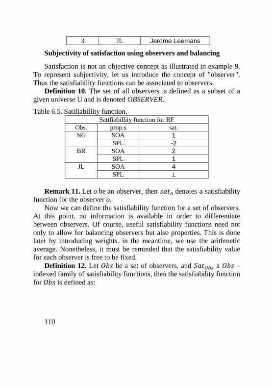
110

3 JL Jerome Leemans

Subjectivity of satisfaction using observers and balancing

Satisfaction is not an objective concept as illustrated in example 9.

To represent subjectivity, let us introduce the concept of "observer".

Thus the satisfiability functions can be associated to observers.

Definition 10. The set of all observers is defined as a subset of a

given universe U and is denoted OBSERVER.

Table 6.5. Satifiabillity function. Satifiabillity function for RF

Obs. prop.s sat.

NG SOA 1

SPL -2

BR SOA 2

SPL 1

JL SOA 4

SPL ⊥

Remark 11. Let o be an observer, then 𝑠𝑎𝑡𝑜 denotes a satisfiability

function for the observer o.

Now we can define the satisfiability function for a set of observers.

At this point, no information is available in order to differentiate

between observers. Of course, useful satisfiability functions need not

only to allow for balancing observers but also properties. This is done

later by introducing weights. in the meantime, we use the arithmetic

average. Nonetheless, it must be reminded that the satisfiability value

for each observer is free to be fixed.

Definition 12. Let 𝑂𝑏𝑠 be a set of observers, and 𝑆𝑎𝑡𝑂𝑏𝑠 a 𝑂𝑏𝑠 –

indexed family of satisfiability functions, then the satisfiability function

for 𝑂𝑏𝑠 is defined as:

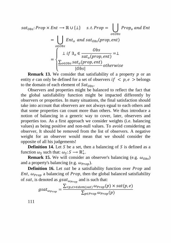
111

𝑠𝑎𝑡𝑂𝑏𝑠: 𝑃𝑟𝑜𝑝 × 𝐸𝑛𝑡 ⟶ ℝ ∪ {⊥} 𝑠. 𝑡. 𝑃𝑟𝑜𝑝 = ⋃ 𝑃𝑟𝑜𝑝𝑜 𝑎𝑛𝑑 𝐸𝑛𝑡

𝑜∈𝑂𝑏𝑠

= ⋃ 𝐸𝑛𝑡𝑜

𝑜∈𝑂𝑏𝑠

𝑎𝑛𝑑 𝑠𝑎𝑡𝑂𝑏𝑠(𝑝𝑟𝑜𝑝, 𝑒𝑛𝑡)

=

{

⊥ 𝑖𝑓 ∃𝑜 ∈

𝑂𝑏𝑠

𝑠𝑎𝑡𝑜(𝑝𝑟𝑜𝑝, 𝑒𝑛𝑡)=⊥

∑ 𝑠𝑎𝑡𝑜(𝑝𝑟𝑜𝑝, 𝑒𝑛𝑡)𝑜∈𝑂𝑏𝑠

|𝑂𝑏𝑠|𝑜𝑡ℎ𝑒𝑟𝑤𝑖𝑠𝑒

Remark 13. We consider that satisfiability of a property 𝑝 or an

entity 𝑒 can only be defined for a set of observers 𝑖𝑓 < 𝑝, 𝑒 > belongs

to the domain of each element of 𝑆𝑎𝑡𝑂𝑏𝑠. Observers and properties might be balanced to reflect the fact that

the global satisfiability function might be impacted differently by

observers or properties. In many situations, the final satisfaction should

take into account that observers are not always egual to each others and

that some properties can count more than others. We thus introduce a

notion of balancing in a generic way to cover, later, observers and

properties too. As a first approach we consider weights (i.e. balancing

values) as being positive and non-null values. To avoid considering an

observer, It should be removed from the list of observers. A negative

weight for an observer would mean that we should consider the

opposite of all his judgements!

Definition 14. Let 𝑆 be a set, then a balancing of 𝑆 is defined as a

function 𝜔𝑆 such that: 𝜔𝑆: 𝑆 ⟶ ℝ+∗ .

Remark 15. We will consider an observer's balancing (e.g. 𝜔𝑂𝑏𝑠) and a property's balancing (e.g. 𝜔𝑃𝑟𝑜𝑝).

Definition 16. Let 𝑠𝑎𝑡 be a satisfiability function over 𝑃𝑟𝑜𝑝 and

𝐸𝑛𝑡, 𝜔𝑃𝑟𝑜𝑝 a balancing of 𝑃𝑟𝑜𝑝, then the global balanced satisfiability

of 𝑠𝑎𝑡, is denoted as 𝑔𝑠𝑎𝑡𝜔𝑃𝑟𝑜𝑝 and is such that:

𝑔𝑠𝑎𝑡𝜔𝑃𝑟𝑜𝑝 =∑ 𝜔𝑃𝑟𝑜𝑝(𝑝) × 𝑠𝑎𝑡(𝑝, 𝑒)<𝑝,𝑒>∈𝑑𝑜𝑚(𝑠𝑎𝑡)

∑ 𝜔𝑃𝑟𝑜𝑝(𝑝)𝑝∈𝑃𝑟𝑜𝑝

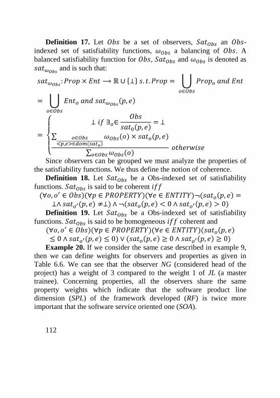
112

Definition 17. Let 𝑂𝑏𝑠 be a set of observers, 𝑆𝑎𝑡𝑂𝑏𝑠 an 𝑂𝑏𝑠-indexed set of satisfiability functions, 𝜔𝑂𝑏𝑠 a balancing of 𝑂𝑏𝑠. A

balanced satisfiability function for 𝑂𝑏𝑠, 𝑆𝑎𝑡𝑂𝑏𝑠 and 𝜔𝑂𝑏𝑠 is denoted as

𝑠𝑎𝑡𝜔𝑂𝑏𝑠 and is such that:

𝑠𝑎𝑡𝜔𝑂𝑏𝑠 : 𝑃𝑟𝑜𝑝 × 𝐸𝑛𝑡 ⟶ ℝ ∪ {⊥} 𝑠. 𝑡. 𝑃𝑟𝑜𝑝 = ⋃ 𝑃𝑟𝑜𝑝𝑜 𝑎𝑛𝑑 𝐸𝑛𝑡

𝑜∈𝑂𝑏𝑠

= ⋃ 𝐸𝑛𝑡𝑜 𝑎𝑛𝑑 𝑠𝑎𝑡𝜔𝑂𝑏𝑠(𝑝, 𝑒)

𝑜∈𝑂𝑏𝑠

=

{

⊥ 𝑖𝑓 ∃𝑜∈

𝑂𝑏𝑠

𝑠𝑎𝑡0(𝑝, 𝑒)= ⊥

∑ 𝜔𝑂𝑏𝑠(𝑜) × 𝑠𝑎𝑡𝑜(𝑝, 𝑒)𝑜∈𝑂𝑏𝑠<𝑝,𝑒>∈𝑑𝑜𝑚(𝑠𝑎𝑡𝑜)

∑ 𝜔𝑂𝑏𝑠(𝑜)𝑜∈𝑂𝑏𝑠 𝑜𝑡ℎ𝑒𝑟𝑤𝑖𝑠𝑒

Since observers can be grouped we must analyze the properties of

the satisfiability functions. We thus define the notion of coherence.

Definition 18. Let 𝑆𝑎𝑡𝑂𝑏𝑠 be a Obs-indexed set of satisfiability

functions. 𝑆𝑎𝑡𝑂𝑏𝑠 is said to be coherent 𝑖𝑓𝑓

(∀𝑜, 𝑜′ ∈ 𝑂𝑏𝑠)(∀𝑝 ∈ 𝑃𝑅𝑂𝑃𝐸𝑅𝑇𝑌)(∀𝑒 ∈ 𝐸𝑁𝑇𝐼𝑇𝑌)¬(𝑠𝑎𝑡𝑜(𝑝, 𝑒) =

⊥∧ 𝑠𝑎𝑡𝑜′(𝑝, 𝑒) ≠⊥) ∧ ¬(𝑠𝑎𝑡𝑜(𝑝, 𝑒) < 0 ∧ 𝑠𝑎𝑡𝑜′(𝑝, 𝑒) > 0) Definition 19. Let 𝑆𝑎𝑡𝑂𝑏𝑠 be a Obs-indexed set of satisfiability

functions. 𝑆𝑎𝑡𝑂𝑏𝑠 is said to be homogeneous 𝑖𝑓𝑓 coherent and

(∀𝑜, 𝑜′ ∈ 𝑂𝑏𝑠)(∀𝑝 ∈ 𝑃𝑅𝑂𝑃𝐸𝑅𝑇𝑌)(∀𝑒 ∈ 𝐸𝑁𝑇𝐼𝑇𝑌)(𝑠𝑎𝑡𝑜(𝑝, 𝑒) ≤ 0 ∧ 𝑠𝑎𝑡𝑜′(𝑝, 𝑒) ≤ 0) ∨ (𝑠𝑎𝑡𝑜(𝑝, 𝑒) ≥ 0 ∧ 𝑠𝑎𝑡𝑜′(𝑝, 𝑒) ≥ 0)

Example 20. If we consider the same case described in example 9,

then we can define weights for observers and properties as given in

Table 6.6. We can see that the observer NG (considered head of the

project) has a weight of 3 compared to the weight 1 of JL (a master

trainee). Concerning properties, all the observers share the same

property weights which indicate that the software product line

dimension (SPL) of the framework developed (RF) is twice more

important that the software service oriented one (SOA).

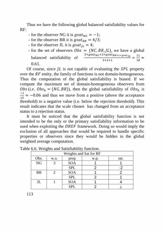
113

Thus we have the following global balanced satisfiability values for

RF:

- for the observer NG it is 𝑔𝑠𝑎𝑡𝑁𝐺 = −1;

- for the observer BR it is 𝑔𝑠𝑎𝑡𝐵𝑅 = 4/3;

- for the observer JL it is 𝑔𝑠𝑎𝑡𝐽𝐿 = 4;

- for the set of observers 𝑂𝑏𝑠 = {𝑁𝐶, 𝐵𝑅, 𝐽𝐿}, we have a global

balanced satisfiability of 3×𝑔𝑠𝑎𝑡𝑁𝐺+2×𝑔𝑠𝑎𝑡𝐵𝑅+1×𝑔𝑠𝑎𝑡𝐽𝐿

3+2+1=11

18≈

0.61.

Of course, since 𝐽𝐿 is not capable of evaluating the 𝑆𝑃𝐿 property

over the 𝑅𝐹 entity, the family of functions is not domain-homogeneous.

Thus the computation of the global satisfiability is biased. If we

compute the maximum set of domain-homogeneous observers from

𝑂𝑏𝑠 (i.e. 𝑂𝑏𝑠ℎ = {𝑁𝐺, 𝐵𝑅}), then the global satisfiability of 𝑂𝑏𝑠ℎ is −1

15≈ −0.06 and thus we move from a positive (above the acceptance

threshold) to a negative value (i.e. below the rejection threshold). This

result indicates that the scale chosen has changed from an acceptance

status to a rejection status.

It must be noticed that the global satisfiability function is not

intended to be the only or the primary satisfiability information to be

used when exploiting the 𝐷𝑅𝐸𝐹 framework. Doing so would imply the

exclusion of all approaches that would be required to handle specific

properties or observers since they would be hidden in the global

weighted average computation.

Table 6.6. Weights and Satisfiability function. Weights and Sat for RF

Obs. w.o. prop w.p. sat.

NG 3 SOA 1 1

SPL 2 -2

BR 2 SOA 1 2

SPL 2 1

JL 1 SOA 1 4

SPL 2 ⊥

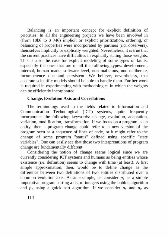
114

Balancing is an important concept for explicit definition of

priorities. In all the engineering projects we have been involved in

(from 10k€ to 3 M€) implicit or explicit prioritization, ordering, or

balancing of properties were incorporated by partners (i.d. observers),

themselves implicitly or explicitly weighted. Nevertheless, it is true that

the current practices have difficulties in explicitly stating those weights.

This is also the case for explicit modeling of some types of faults,

especially the ones that are of all the following types: development,

internal, human made, software level, non malicious, non deliberate,

incompetence due and persistent. We believe, nevertheless, that

accurate scientific models should be able to handle them. Further work

is required in experimenting with methodologies in which the weights

can be efficiently incorporated.

Change, Evolution Axis and Correlations

The terminology used in the fields related to Information and

Communication Technological (ICT) systems, quite frequently

incorporates the following keywords: change, evolution, adaptation,

variation, modification, transformation. If we focus on a program as an

entity, then a program change could refer to a new version of the

program seen as a sequence of lines of code, or it might refer to the

change of some program "status" defined using specific "state

variables". One can easily see that those two interpretations of program

change are fundamentally different.

Considering the notion of change seems logical since we are

currently considering ICT systems and humans as being entities whose

existence (i.e. definition) seems to change with time (at least). A first

simple approximation, then, would be to define change as the

difference between two definitions of two entities distributed over a

common evolution axis. As an example, let consider 𝑝1 as a simple

imperative program sorting a list of integers using the bubble algorithm

and 𝑝2 using a guick sort algorithm. If we consider 𝑝1 and 𝑝2 as

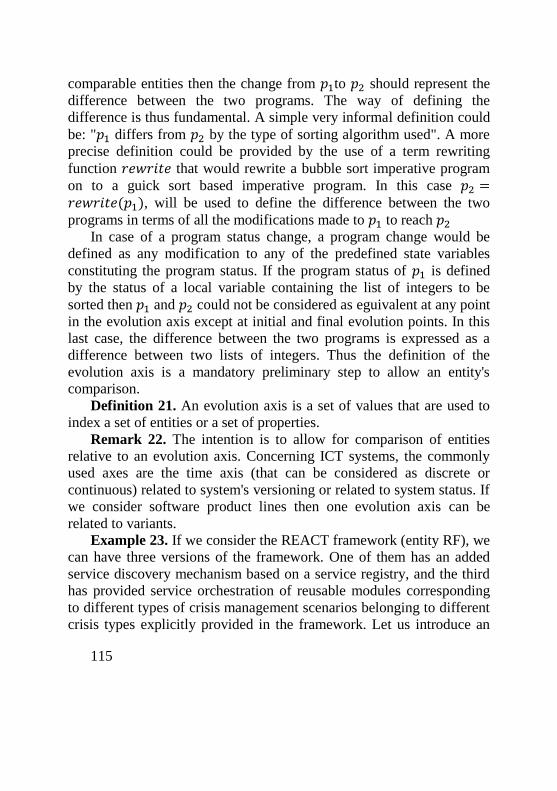
115

comparable entities then the change from 𝑝1to 𝑝2 should represent the

difference between the two programs. The way of defining the

difference is thus fundamental. A simple very informal definition could

be: "𝑝1 differs from 𝑝2 by the type of sorting algorithm used". A more

precise definition could be provided by the use of a term rewriting

function 𝑟𝑒𝑤𝑟𝑖𝑡𝑒 that would rewrite a bubble sort imperative program

on to a guick sort based imperative program. In this case 𝑝2 =𝑟𝑒𝑤𝑟𝑖𝑡𝑒(𝑝1), will be used to define the difference between the two

programs in terms of all the modifications made to 𝑝1 to reach 𝑝2

In case of a program status change, a program change would be

defined as any modification to any of the predefined state variables

constituting the program status. If the program status of 𝑝1 is defined

by the status of a local variable containing the list of integers to be

sorted then 𝑝1 and 𝑝2 could not be considered as eguivalent at any point

in the evolution axis except at initial and final evolution points. In this

last case, the difference between the two programs is expressed as a

difference between two lists of integers. Thus the definition of the

evolution axis is a mandatory preliminary step to allow an entity's

comparison.

Definition 21. An evolution axis is a set of values that are used to

index a set of entities or a set of properties.

Remark 22. The intention is to allow for comparison of entities

relative to an evolution axis. Concerning ICT systems, the commonly

used axes are the time axis (that can be considered as discrete or

continuous) related to system's versioning or related to system status. If

we consider software product lines then one evolution axis can be

related to variants.

Example 23. If we consider the REACT framework (entity RF), we

can have three versions of the framework. One of them has an added

service discovery mechanism based on a service registry, and the third

has provided service orchestration of reusable modules corresponding

to different types of crisis management scenarios belonging to different

crisis types explicitly provided in the framework. Let us introduce an

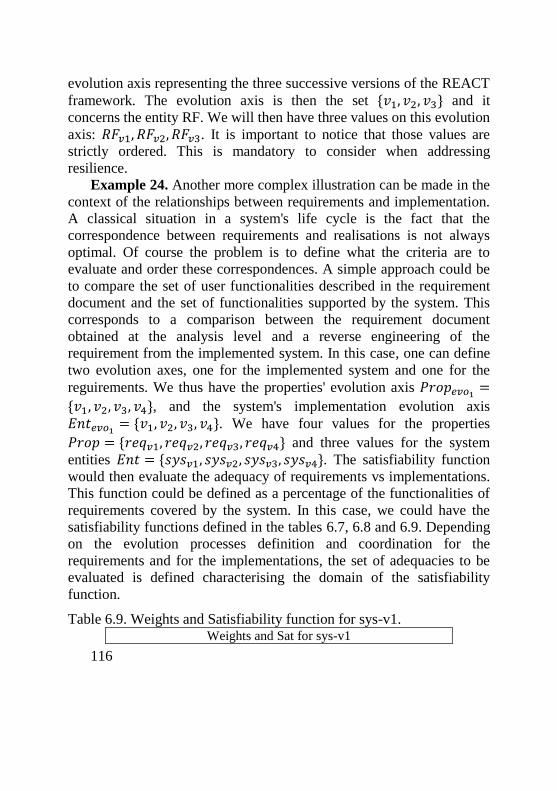
116

evolution axis representing the three successive versions of the REACT

framework. The evolution axis is then the set {𝑣1, 𝑣2, 𝑣3} and it

concerns the entity RF. We will then have three values on this evolution

axis: 𝑅𝐹𝑣1, 𝑅𝐹𝑣2, 𝑅𝐹𝑣3. It is important to notice that those values are

strictly ordered. This is mandatory to consider when addressing

resilience.

Example 24. Another more complex illustration can be made in the

context of the relationships between requirements and implementation.

A classical situation in a system's life cycle is the fact that the

correspondence between requirements and realisations is not always

optimal. Of course the problem is to define what the criteria are to

evaluate and order these correspondences. A simple approach could be

to compare the set of user functionalities described in the requirement

document and the set of functionalities supported by the system. This

corresponds to a comparison between the requirement document

obtained at the analysis level and a reverse engineering of the

requirement from the implemented system. In this case, one can define

two evolution axes, one for the implemented system and one for the

reguirements. We thus have the properties' evolution axis 𝑃𝑟𝑜𝑝𝑒𝑣𝑜1 =

{𝑣1, 𝑣2, 𝑣3, 𝑣4}, and the system's implementation evolution axis

𝐸𝑛𝑡𝑒𝑣𝑜1 = {𝑣1, 𝑣2, 𝑣3, 𝑣4}. We have four values for the properties

𝑃𝑟𝑜𝑝 = {𝑟𝑒𝑞𝑣1, 𝑟𝑒𝑞𝑣2, 𝑟𝑒𝑞𝑣3, 𝑟𝑒𝑞𝑣4} and three values for the system

entities 𝐸𝑛𝑡 = {𝑠𝑦𝑠𝑣1, 𝑠𝑦𝑠𝑣2, 𝑠𝑦𝑠𝑣3, 𝑠𝑦𝑠𝑣4}. The satisfiability function

would then evaluate the adequacy of requirements vs implementations.

This function could be defined as a percentage of the functionalities of

requirements covered by the system. In this case, we could have the

satisfiability functions defined in the tables 6.7, 6.8 and 6.9. Depending

on the evolution processes definition and coordination for the

requirements and for the implementations, the set of adequacies to be

evaluated is defined characterising the domain of the satisfiability

function.

Table 6.9. Weights and Satisfiability function for sys-v1. Weights and Sat for sys-v1

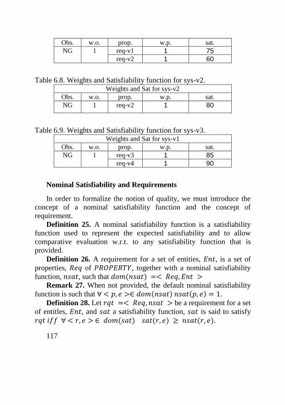
117

Obs. w.o. prop. w.p. sat.

NG 1 req-v1 1 75

req-v2 1 60

Table 6.8. Weights and Satisfiability function for sys-v2. Weights and Sat for sys-v2

Obs. w.o. prop. w.p. sat.

NG 1 req-v2 1 80

Table 6.9. Weights and Satisfiability function for sys-v3. Weights and Sat for sys-v1

Obs. w.o. prop. w.p. sat.

NG 1 req-v3 1 85

req-v4 1 90

Nominal Satisfiability and Requirements

In order to formalize the notion of quality, we must introduce the

concept of a nominal satisfiability function and the concept of

requirement.

Definition 25. A nominal satisfiability function is a satisfiability

function used to represent the expected satisfiability and to allow

comparative evaluation w.r.t. to any satisfiability function that is

provided.

Definition 26. A requirement for a set of entities, 𝐸𝑛𝑡, is a set of

properties, 𝑅𝑒𝑞 of 𝑃𝑅𝑂𝑃𝐸𝑅𝑇𝑌, together with a nominal satisfiability

function, 𝑛𝑠𝑎𝑡, such that 𝑑𝑜𝑚(𝑛𝑠𝑎𝑡) =< 𝑅𝑒𝑞, 𝐸𝑛𝑡 >

Remark 27. When not provided, the default nominal satisfiability

function is such that ∀ < 𝑝, 𝑒 >∈ 𝑑𝑜𝑚(𝑛𝑠𝑎𝑡) 𝑛𝑠𝑎𝑡(𝑝, 𝑒) = 1.

Definition 28. Let 𝑟𝑞𝑡 =< 𝑅𝑒𝑞, 𝑛𝑠𝑎𝑡 > be a requirement for a set

of entitles, 𝐸𝑛𝑡, and 𝑠𝑎𝑡 a satisfiability function, 𝑠𝑎𝑡 is said to satisfy

𝑟𝑞𝑡 𝑖𝑓𝑓 ∀ < 𝑟, 𝑒 > ∈ 𝑑𝑜𝑚(𝑠𝑎𝑡) 𝑠𝑎𝑡(𝑟, 𝑒) ≥ 𝑛𝑠𝑎𝑡(𝑟, 𝑒).

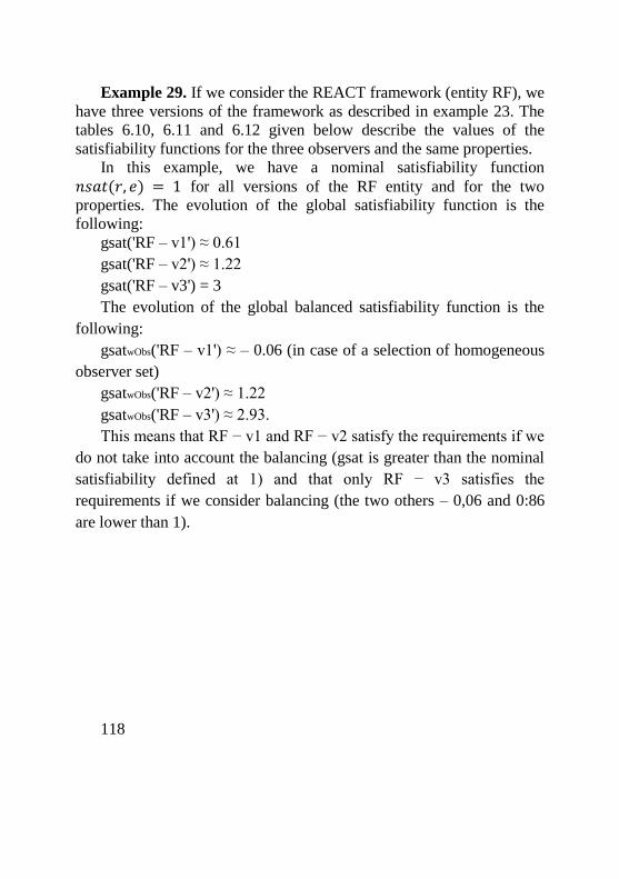
118

Example 29. If we consider the REACT framework (entity RF), we

have three versions of the framework as described in example 23. The

tables 6.10, 6.11 and 6.12 given below describe the values of the

satisfiability functions for the three observers and the same properties.

In this example, we have a nominal satisfiability function

𝑛𝑠𝑎𝑡(𝑟, 𝑒) = 1 for all versions of the RF entity and for the two

properties. The evolution of the global satisfiability function is the

following:

gsat('RF – v1') ≈ 0.61

gsat('RF – v2') ≈ 1.22

gsat('RF – v3') = 3

The evolution of the global balanced satisfiability function is the

following:

gsatwObs('RF – v1') ≈ – 0.06 (in case of a selection of homogeneous

observer set)

gsatwObs('RF – v2') ≈ 1.22

gsatwObs('RF – v3') ≈ 2.93.

This means that RF − v1 and RF − v2 satisfy the requirements if we

do not take into account the balancing (gsat is greater than the nominal

satisfiability defined at 1) and that only RF − v3 satisfies the

requirements if we consider balancing (the two others – 0,06 and 0:86

are lower than 1).

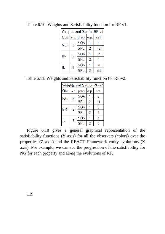
119

Table 6.10. Weights and Satisfiability function for RF-v1.

Table 6.11. Weights and Satisfiability function for RF-v2.

Figure 6.18 gives a general graphical representation of the

satisfiability functions (Y axis) for all the observers (colors) over the

properties (Z axis) and the REACT Framework entity evolutions (X

axis). For example, we can see the progression of the satisfiability for

NG for each property and along the evolutions of RF.

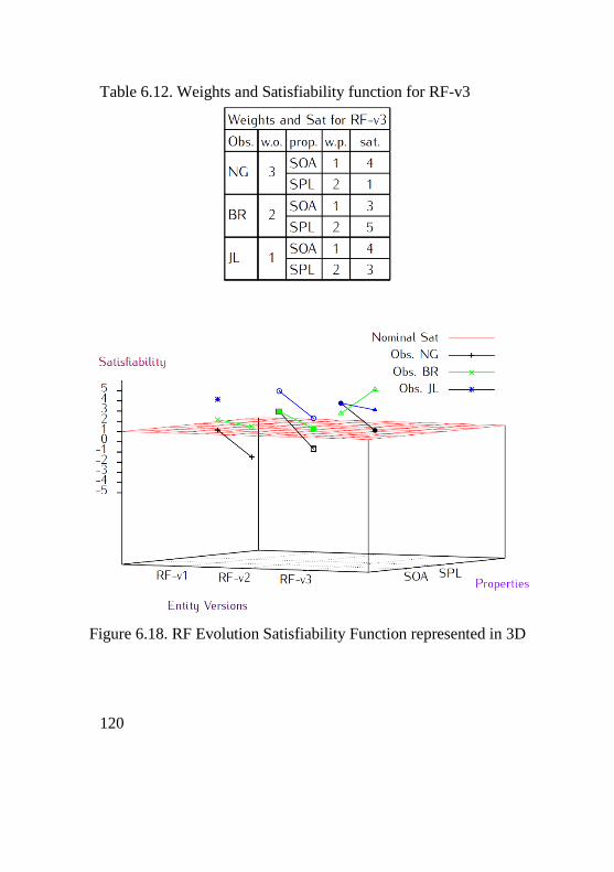
120

Table 6.12. Weights and Satisfiability function for RF-v3

Figure 6.18. RF Evolution Satisfiability Function represented in 3D

121

Tolerance, Preservation, Improvement and Degradation

In order to address the main concepts of dependability, we propose

to define four basic concepts in our formal framework: tolerance,

preservation, improvement and degradation. We consider that there is

no universal notion of quality but rather that quality is a subjective

notion relative to a set of properties that represent the expectation on a

specific entity.

Definition 30.

A tolerance threshold is defined as a satisfiability function.

Tolerance threshold functions are used to represent the lower bound

that defines the tolerance margin for satisfiability functions w.r.t. a

nominal satisfiability function.

Remark 31.

Tolerance threshold functions will be denoted as tolsat.

The tolerance margin is the space between nsat and tolsat (see

Figure 6.19).

Intolerance is characterised by nsat = tolsat.

Definition 32.

A preservation is defined as constancy in a satisfiability function

w.r.t. an evolution axis.

Definition 33.

An improvement is defined as an increase in a satisfiability function

w.r.t. an evolution axis.

Definition 34.

A degradation is defined as a decrease in a satisfiability function

w.r.t. an evolution axis.

Remark 35.

Preservation (resp.improvement, degradation) might be observed

relative to a nominal satisfiability and tolerance threshold in order to

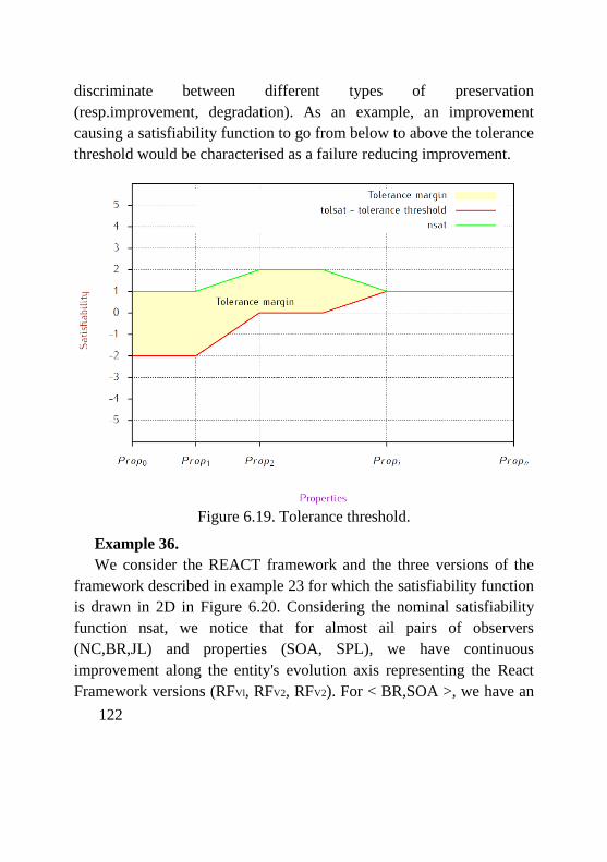
122

discriminate between different types of preservation

(resp.improvement, degradation). As an example, an improvement

causing a satisfiability function to go from below to above the tolerance

threshold would be characterised as a failure reducing improvement.

Figure 6.19. Tolerance threshold.

Example 36.

We consider the REACT framework and the three versions of the

framework described in example 23 for which the satisfiability function

is drawn in 2D in Figure 6.20. Considering the nominal satisfiability

function nsat, we notice that for almost ail pairs of observers

(NC,BR,JL) and properties (SOA, SPL), we have continuous

improvement along the entity's evolution axis representing the React

Framework versions (RFVl, RFV2, RFV2). For < BR,SOA >, we have an

123

improvement from RFVl to RFV2 and a preservation from RFV2 to RFV2 .

For < JL,SOA >, we have an improvement from RFVl to RFV2 and a

degradation from RFV2 to RFV2. If we now consider the varying

nominal satisfiability function, nsat', we observe that there is no

improvement but preservation for < BR,SOA > (and < NC,SPL >,<

JL,SOA >) RFVl to RFV2.

Tolerance and Failure

Based on the previous definition of tolerance margin, we now

address the notions of tolerance and failure. Both concepts are related

to the satisfaction of a property over an entity given a nominal

satisfiability and tolerance threshold functions.

Definition 37.

Given sat, a satisfiability function, and tolsat, a tolerance threshold,

a failure is defined as a tuple < r,ent >ϵ dom(sat) Ո dom(tolsat) such

that: sat(r, ent)≤tolsat(r, ent).

Remark 38.

1. We will write fail(r, ent) to denote the failure < r, ent >

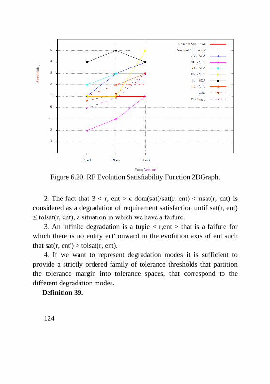
124

Figure 6.20. RF Evolution Satisfiability Function 2DGraph.

2. The fact that 3 < r, ent > ϵ dom(sat)/sat(r, ent) < nsat(r, ent) is

considered as a degradation of requirement satisfaction untif sat(r, ent)

≤ tolsat(r, ent), a situation in which we have a faifure.

3. An infinite degradation is a tupie < r,ent > that is a faifure for

which there is no entity ent' onward in the evofution axis of ent such

that sat(r, ent') > tolsat(r, ent).

4. If we want to represent degradation modes it is sufficient to

provide a strictly ordered family of tolerance thresholds that partition

the tolerance margin into tolerance spaces, that correspond to the

different degradation modes.

Definition 39.

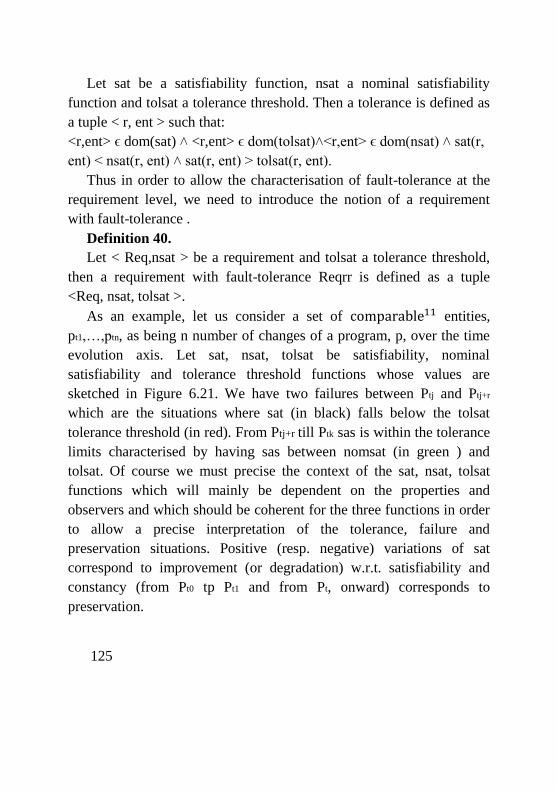
125

Let sat be a satisfiability function, nsat a nominal satisfiability

function and tolsat a tolerance threshold. Then a tolerance is defined as

a tuple < r, ent > such that:

<r,ent> ϵ dom(sat) ˄ <r,ent> ϵ dom(tolsat)˄<r,ent> ϵ dom(nsat) ˄ sat(r,

ent) < nsat(r, ent) ˄ sat(r, ent) > tolsat(r, ent).

Thus in order to allow the characterisation of fault-tolerance at the

requirement level, we need to introduce the notion of a requirement

with fault-tolerance .

Definition 40.

Let < Req,nsat > be a requirement and tolsat a tolerance threshold,

then a requirement with fault-tolerance Reqrr is defined as a tuple

<Req, nsat, tolsat >.

As an example, let us consider a set of comparable11 entities,

pt1,…,ptn, as being n number of changes of a program, p, over the time

evolution axis. Let sat, nsat, tolsat be satisfiability, nominal

satisfiability and tolerance threshold functions whose values are

sketched in Figure 6.21. We have two failures between Ptj and Ptj+r

which are the situations where sat (in black) falls below the tolsat

tolerance threshold (in red). From Ptj+r till Ptk sas is within the tolerance

limits characterised by having sas between nomsat (in green ) and

tolsat. Of course we must precise the context of the sat, nsat, tolsat

functions which will mainly be dependent on the properties and

observers and which should be coherent for the three functions in order

to allow a precise interpretation of the tolerance, failure and

preservation situations. Positive (resp. negative) variations of sat

correspond to improvement (or degradation) w.r.t. satisfiability and

constancy (from Pt0 tp Pt1 and from Pt, onward) corresponds to

preservation.

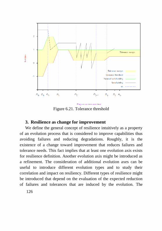
126

Figure 6.21. Tolerance threshold

3. Resilience as change for improvement

We define the general concept of resilience intuitively as a property

of an evolution process that is considered to improve capabilities thus

avoiding failures and reducing degradations. Roughly, it is the

existence of a change toward improvement that reduces failures and

tolerance needs. This fact implies that at least one evolution axis exists

for resilience definition. Another evolution axis might be introduced as

a refinement. The consideration of additional evolution axes can be

useful to introduce different evolution types and to study their

correlation and impact on resiliency. Different types of resilience might

be introduced that depend on the evaluation of the expected reduction

of failures and tolerances that are induced by the evolution. The

127

properties used for the evaluation of the satisfiability function define

observation points. Thus an observation axis could also be introduced

to classify the observation points used for the evaluation of failures and

degradations and their change over the chosen evolution axes. The

explicit concep¬tualisation of evolutions and observations is a

fundamental task to allow for good dependability and resilience

evaluation.

The next definitions are fundamental in our framework. The first

introduces: tolmax as the maximum possible level of tolerance needed.

It is defined based on the differences between the expected lowest

acceptable satisfiability levels (in Figure 6.23 it is the yellow surface);

stol represents the total quantity of tolerance deduced from the effective

satisfiability all along the evolution axis (in Figure 6.23 it is the green

surface); /to/ is the proportion of the two previous quantities. The

second definition introduces a variation of the required tolerance levels

between two evolutions (successive or not). The third definition focuses

on failures and introduces: 1) a failure level that indicates the failure

grade for a given property and entity evolution (in Figure 6.23 it is the

distance between the red curve and any point of an entity version curve

that goes below it); 2) qfail represents the number of times an entity is

failing (goes below the tolerance threshold) all along its evolution axis;

and 3) sfail quantifies the level of failure as for stol. The fourth

definition introduces the variation quantities in terms of number of

failures ( ∆qfail) and failure level ( ∆fail).

Definition 41.

Let entv be an entity, and ev = {1,…,m} be an evolution axis for

entv. Let sat be a satisfiability function defined over entv and over a set

of properties Prop, nsat a nominal satisfiability function and tolsat a

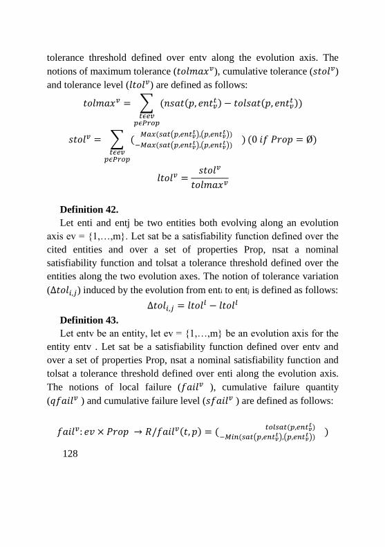
128

tolerance threshold defined over entv along the evolution axis. The

notions of maximum tolerance (𝑡𝑜𝑙𝑚𝑎𝑥𝑣), cumulative tolerance (𝑠𝑡𝑜𝑙𝑣)

and tolerance level (𝑙𝑡𝑜𝑙𝑣) are defined as follows:

𝑡𝑜𝑙𝑚𝑎𝑥𝑣 = ∑ (𝑛𝑠𝑎𝑡(𝑝, 𝑒𝑛𝑡𝑣𝑡) − 𝑡𝑜𝑙𝑠𝑎𝑡(𝑝, 𝑒𝑛𝑡𝑣

𝑡))𝑡𝜖𝑒𝑣𝑝𝜖𝑃𝑟𝑜𝑝

𝑠𝑡𝑜𝑙𝑣 = ∑ (−𝑀𝑎𝑥(𝑠𝑎𝑡(𝑝,𝑒𝑛𝑡𝑣

𝑡),(𝑝,𝑒𝑛𝑡𝑣𝑡))

𝑀𝑎𝑥(𝑠𝑎𝑡(𝑝,𝑒𝑛𝑡𝑣𝑡),(𝑝,𝑒𝑛𝑡𝑣

𝑡)))

𝑡𝜖𝑒𝑣𝑝𝜖𝑃𝑟𝑜𝑝

(0 𝑖𝑓 𝑃𝑟𝑜𝑝 = Ø)

𝑙𝑡𝑜𝑙𝑣 =𝑠𝑡𝑜𝑙𝑣

𝑡𝑜𝑙𝑚𝑎𝑥𝑣

Definition 42.

Let enti and entj be two entities both evolving along an evolution

axis ev = {1,…,m}. Let sat be a satisfiability function defined over the

cited entities and over a set of properties Prop, nsat a nominal

satisfiability function and tolsat a tolerance threshold defined over the

entities along the two evolution axes. The notion of tolerance variation

(∆𝑡𝑜𝑙𝑖,𝑗) induced by the evolution from enti to entj is defined as follows:

∆𝑡𝑜𝑙𝑖,𝑗 = 𝑙𝑡𝑜𝑙𝑙 − 𝑙𝑡𝑜𝑙𝑙

Definition 43.

Let entv be an entity, let ev = {1,…,m} be an evolution axis for the

entity entv . Let sat be a satisfiability function defined over entv and

over a set of properties Prop, nsat a nominal satisfiability function and

tolsat a tolerance threshold defined over enti along the evolution axis.

The notions of local failure (𝑓𝑎𝑖𝑙𝑣 ), cumulative failure quantity

(𝑞𝑓𝑎𝑖𝑙𝑣 ) and cumulative failure level (𝑠𝑓𝑎𝑖𝑙𝑣 ) are defined as follows:

𝑓𝑎𝑖𝑙𝑣: 𝑒𝑣 × 𝑃𝑟𝑜𝑝 → 𝑅/𝑓𝑎𝑖𝑙𝑣(𝑡, 𝑝) = (−𝑀𝑖𝑛(𝑠𝑎𝑡(𝑝,𝑒𝑛𝑡𝑣

𝑡),(𝑝,𝑒𝑛𝑡𝑣𝑡))

𝑡𝑜𝑙𝑠𝑎𝑡(𝑝,𝑒𝑛𝑡𝑣𝑡))

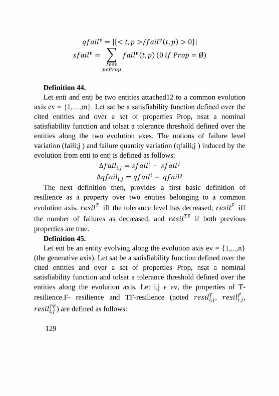
129

𝑞𝑓𝑎𝑖𝑙𝑣 = |{< 𝑡, 𝑝 >/𝑓𝑎𝑖𝑙𝑣(𝑡, 𝑝) > 0}|

𝑠𝑓𝑎𝑖𝑙𝑣 = ∑ 𝑓𝑎𝑖𝑙𝑣(𝑡, 𝑝)𝑡𝜖𝑒𝑣𝑝𝜖𝑃𝑟𝑜𝑝

(0 𝑖𝑓 𝑃𝑟𝑜𝑝 = Ø)

Definition 44.

Let enti and entj be two entities attached12 to a common evolution

axis ev = {1,…,m}. Let sat be a satisfiability function defined over the

cited entities and over a set of properties Prop, nsat a nominal

satisfiability function and tolsat a tolerance threshold defined over the

entities along the two evolution axes. The notions of failure level

variation (faili;j ) and failure quantity variation (qfaili;j ) induced by the

evolution from enti to entj is defined as follows:

∆𝑓𝑎𝑖𝑙𝑖,𝑗 = 𝑠𝑓𝑎𝑖𝑙𝑖 − 𝑠𝑓𝑎𝑖𝑙𝑗

∆𝑞𝑓𝑎𝑖𝑙𝑖,𝑗 = 𝑞𝑓𝑎𝑖𝑙𝑖 − 𝑞𝑓𝑎𝑖𝑙𝑗

The next definition then, provides a first basic definition of

resilience as a property over two entities belonging to a common

evolution axis. 𝑟𝑒𝑠𝑖𝑙𝑇 iff the tolerance level has decreased; 𝑟𝑒𝑠𝑖𝑙𝐹 iff

the number of failures as decreased; and 𝑟𝑒𝑠𝑖𝑙𝑇𝐹 if both previous

properties are true.

Definition 45.

Let ent be an entity evolving along the evolution axis ev = {1,...,n}

(the generative axis). Let sat be a satisfiability function defined over the

cited entities and over a set of properties Prop, nsat a nominal

satisfiability function and tolsat a tolerance threshold defined over the

entities along the evolution axis. Let i,j ϵ ev, the properties of T-

resilience.F- resilience and TF-resilience (noted 𝑟𝑒𝑠𝑖𝑙𝑖,𝑗𝑇 , 𝑟𝑒𝑠𝑖𝑙𝑖,𝑗

𝐹 ,

𝑟𝑒𝑠𝑖𝑙𝑖,𝑗𝑇𝐹) are defined as follows:

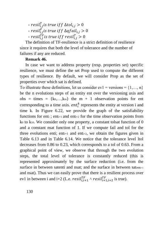
130

- 𝑟𝑒𝑠𝑖𝑙𝑖,𝑗𝑇 𝑖𝑠 𝑡𝑟𝑢𝑒 𝑖𝑓𝑓 ∆𝑡𝑜𝑙𝑖,𝑗 > 0

- 𝑟𝑒𝑠𝑖𝑙𝑖,𝑗𝐹 𝑖𝑠 𝑡𝑟𝑢𝑒 𝑖𝑓𝑓 ∆𝑞𝑓𝑎𝑖𝑙𝑖,𝑗 > 0

- 𝑟𝑒𝑠𝑖𝑙𝑖,𝑗𝑇𝐹𝑖𝑠 𝑡𝑟𝑢𝑒 𝑖𝑓𝑓 𝑟𝑒𝑠𝑖𝑙𝑖,𝑗

𝑇 > 0

The definition of TF-resilience is a strict definition of resilience

since it requires that both the level of tolerance and the number of

failures if any are reduced.

Remark 46.

In case we want to address property (resp. properties set) specific

resilience, we must define the set Prop used to compute the different

types of resilience. By default, we will consider Prop as the set of

properties over which sat is defined.

To illustrate these definitions, let us consider ev1 = versions = {1,…, n}

be the n evolutions steps of an entity ent over the versioning axis and

obs = times = {k0,…,km} the m + 1 observation points for ent

corresponding to a time axis. 𝑒𝑛𝑡𝑖𝑘 represents the entity at version i and

time k. In Figure 6.22, we provide the graph of the satisfiability

functions for enti ; enti+1 and enti+2 for the time observation points from

k0 to k10. We consider only one property, a constant tolsat function of 0

and a constant nsat function of 1. If we compute fail and tol for the

three evolutions enti; enti+1 and enti+2, we obtain the figures given in

Table 6.13 and in Table 6.14. We notice that the tolerance level ltol

decreases from 0.86 to 0.23, which corresponds to a tol of 0.63. From a

graphical point of view, we observe that through the two evolution

steps, the total level of tolerance is constantly reduced (this is

represented approximately by the surface reduction (i.e. from the

surface in between satenti and nsat; and the surface in between satenti+1

and nsat). Thus we can easily prove that there is a resilient process over

ev1 in between i and i+2 (L.e. 𝑟𝑒𝑠𝑖𝑙𝑖,𝑖+1𝑇𝐹 ˄ 𝑟𝑒𝑠𝑖𝑙𝑖+1,𝑖+2

𝑇𝐹 is true).

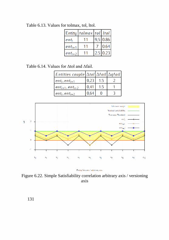
131

Table 6.13. Values for tolmax, tol, ltol.

Table 6.14. Values for ∆tol and ∆fail.

Figure 6.22. Simple Satisfiability correlation arbitrary axis / versioning

axis

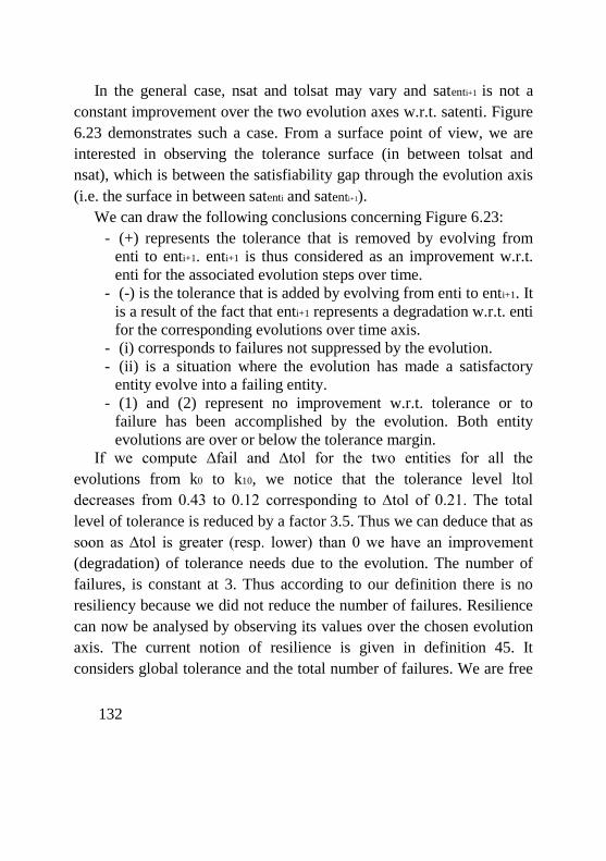
132

In the general case, nsat and tolsat may vary and satenti+1 is not a

constant improvement over the two evolution axes w.r.t. satenti. Figure

6.23 demonstrates such a case. From a surface point of view, we are

interested in observing the tolerance surface (in between tolsat and

nsat), which is between the satisfiability gap through the evolution axis

(i.e. the surface in between satenti and satenti+1).

We can draw the following conclusions concerning Figure 6.23:

- (+) represents the tolerance that is removed by evolving from

enti to enti+1. enti+1 is thus considered as an improvement w.r.t.

enti for the associated evolution steps over time.

- (-) is the tolerance that is added by evolving from enti to enti+1. It

is a result of the fact that enti+1 represents a degradation w.r.t. enti

for the corresponding evolutions over time axis.

- (i) corresponds to failures not suppressed by the evolution.

- (ii) is a situation where the evolution has made a satisfactory

entity evolve into a failing entity.

- (1) and (2) represent no improvement w.r.t. tolerance or to

failure has been accomplished by the evolution. Both entity

evolutions are over or below the tolerance margin.

If we compute ∆fail and ∆tol for the two entities for all the

evolutions from k0 to k10, we notice that the tolerance level ltol

decreases from 0.43 to 0.12 corresponding to ∆tol of 0.21. The total

level of tolerance is reduced by a factor 3.5. Thus we can deduce that as

soon as ∆tol is greater (resp. lower) than 0 we have an improvement

(degradation) of tolerance needs due to the evolution. The number of

failures, is constant at 3. Thus according to our definition there is no

resiliency because we did not reduce the number of failures. Resilience

can now be analysed by observing its values over the chosen evolution

axis. The current notion of resilience is given in definition 45. It

considers global tolerance and the total number of failures. We are free

133

to define specific notions of resilience depending on a number of

interesting parameters. A non-restrictive list could be:

- minimum, maximum delays in term of evolution steps needed to

change ∆tol and ∆qfail.

- use of ∆qfail instead of ∆fail.

- mandatory or optional removal of failures.

- focus on specific properties that might be different between

evolution steps instead of fusing all properties to evaluate the

degradation and the improvement.

- focus on specific evolution intervals at the dynamic evolution

axis level in order to reduce the constraints on resiliency.

- provide constraints on the durability of improvement. The

resilience from enti, to ent j could be reguired to last over the

next generations (no decadence).

-

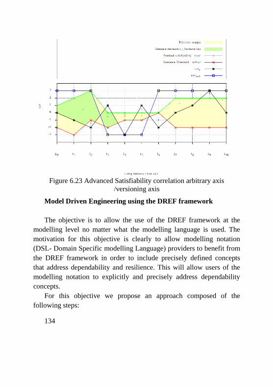
134

Figure 6.23 Advanced Satisfiability correlation arbitrary axis

/versioning axis

Model Driven Engineering using the DREF framework

The objective is to allow the use of the DREF framework at the

modelling level no matter what the modelling language is used. The

motivation for this objective is clearly to allow modelling notation

(DSL- Domain Specific modelling Language) providers to benefit from

the DREF framework in order to include precisely defined concepts

that address dependability and resilience. This will allow users of the

modelling notation to explicitly and precisely address dependability

concepts.

For this objective we propose an approach composed of the

following steps:

135

- Define the meta-model of the targeted DSL using standard meta-

modelling tools i.e. ecore equivalent diagrams [89]. The model

should include meta concepts derived from the DREF meta-

model.

- Define properties, entities and observers at the domain level.

- Define the evolution axis.

- Define the satisfiability functions including the nominal and the

tolerance threshold.

We begin this section by presenting the DREF meta-model.

Subsequently, each of these phases is illustrated using a concrete

example of a toy DSL in the domain of business process modelling.

The DREF meta-model

In this section, let us provide a proposal for introducing DREF

formal framework elements using meta-modelling techniques. The idea

is to propose adequate meta-modelling elements to exploit the

definition of a domain specific language that would be targeted by

potential future users of DREF. In Figure 6.24 provide the model

structure of the DREF meta-model is provided. The idea is that at the

modelling level a DREF model to be composed of 3+1 categories of

models is requested. The first three ones (modes view) are dedicated to

the nominal view, the tolerance view, the fail view. The fourth provides

the satisfiability view. First, it must be noticed that the modes view

could allow one to provide several models per category. This should be

defined in the specific meta-model structure. The models provided will

propose a specific level of the separation of focus of these views. This

means that for a specific DSL the modelling elements for each of these

views might be strongly separated while in some other approaches they

might be fused. It will be up to the meta-model designer to define the

level of separation of concerns that is required.

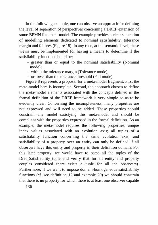
136

In the following example, one can observe an approach for defining

the level of separation of perspectives concerning a DREF extension of

some BPMN like meta-model. The example provides a clear separation

of modelling elements dedicated to nominal satisfiability, tolerance

margin and failures (Figure 18). In any case, at the semantic level, these

views must be implemented for having a means to determine if the

satisfiability function should be:

- greater than or equal to the nominal satisfiability (Nominal

mode);

- within the tolerance margin (Tolerance mode);

- or lower than the tolerance threshold (Fail mode).

Figure 8 represents a proposal for a meta-model fragment. First the

meta-model here is incomplete. Second, the approach chosen to define

the meta-model elements associated with the concepts defined in the

formal definition of the DREF framework is very simple so as to be

evidently clear. Concerning the incompleteness, many properties are

not expressed and will need to be added. These properties should

constrain any model satisfying this meta-model and should be

compliant with the properties expressed in the formal definition. As an

example, the meta-model requires the following properties: unique

index values associated with an evolution axis; all tuples of a

satisfiability function concerning the same evolution axis; and

satisfiability of a property over an entity can only be defined if all

observers have this entity and property in their definition domain. For

this later property, we would have to parse all the tuples of the

Dref_Satisfiability_tuple and verify that for all entity and property

couples considered there exists a tuple for all the observers).

Furthermore, if we want to impose domain-homogeneous satisfiability

functions (cf. see definition 12 and example 20) we should constrain

that there is no property for which there is at least one observer capable

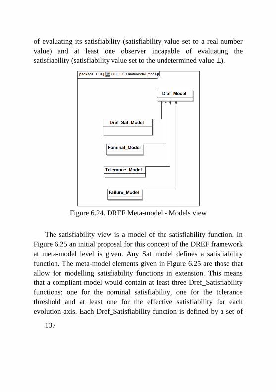
137

of evaluating its satisfiability (satisfiability value set to a real number

value) and at least one observer incapable of evaluating the

satisfiability (satisfiability value set to the undetermined value ⊥).

Figure 6.24. DREF Meta-model - Models view

The satisfiability view is a model of the satisfiability function. In

Figure 6.25 an initial proposal for this concept of the DREF framework

at meta-model level is given. Any Sat_model defines a satisfiability

function. The meta-model elements given in Figure 6.25 are those that

allow for modelling satisfiability functions in extension. This means

that a compliant model would contain at least three Dref_Satisfiability

functions: one for the nominal satisfiability, one for the tolerance

threshold and at least one for the effective satisfiability for each

evolution axis. Each Dref_Satisfiability function is defined by a set of

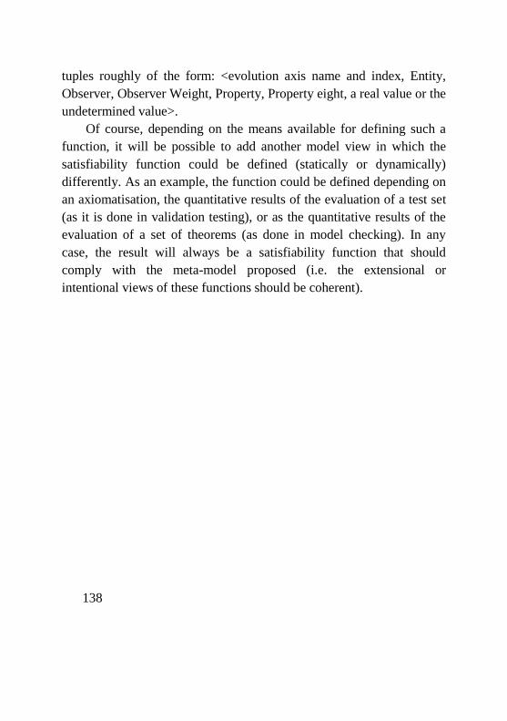
138

tuples roughly of the form: <evolution axis name and index, Entity,

Observer, Observer Weight, Property, Property eight, a real value or the

undetermined value>.

Of course, depending on the means available for defining such a

function, it will be possible to add another model view in which the

satisfiability function could be defined (statically or dynamically)

differently. As an example, the function could be defined depending on

an axiomatisation, the quantitative results of the evaluation of a test set

(as it is done in validation testing), or as the quantitative results of the

evaluation of a set of theorems (as done in model checking). In any

case, the result will always be a satisfiability function that should

comply with the meta-model proposed (i.e. the extensional or

intentional views of these functions should be coherent).

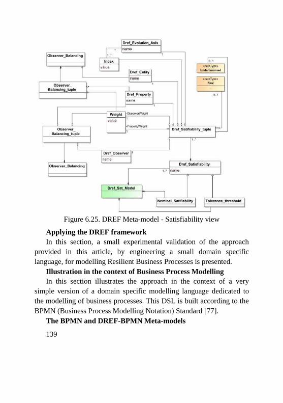
139

Figure 6.25. DREF Meta-model - Satisfiability view

Applying the DREF framework

In this section, a small experimental validation of the approach

provided in this article, by engineering a small domain specific

language, for modelling Resilient Business Processes is presented.

Illustration in the context of Business Process Modelling

In this section illustrates the approach in the context of a very

simple version of a domain specific modelling language dedicated to

the modelling of business processes. This DSL is built according to the

BPMN (Business Process Modelling Notation) Standard [77].

The BPMN and DREF-BPMN Meta-models

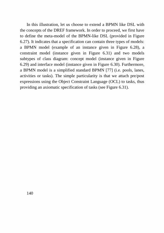
140

In this illustration, let us choose to extend a BPMN like DSL with

the concepts of the DREF framework. In order to proceed, we first have

to define the meta-model of the BPMN-like DSL (provided in Figure

6.27). It indicates that a specification can contain three types of models:

a BPMN model (example of an instance given in Figure 6.28), a

constraint model (instance given in Figure 6.31) and two models

subtypes of class diagram: concept model (instance given in Figure

6.29) and interface model (instance given in Figure 6.30). Furthermore,

a BPMN model is a simplified standard BPMN [77] (i.e. pools, lanes,

activities or tasks). The simple particularity is that we attach pre/post

expressions using the Object Constraint Language (OCL) to tasks, thus

providing an axiomatic specification of tasks (see Figure 6.31).

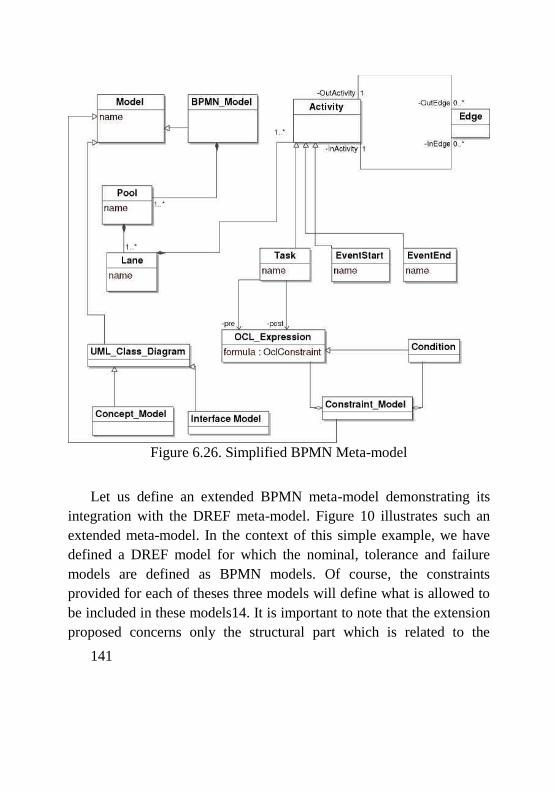
141

Figure 6.26. Simplified BPMN Meta-model

Let us define an extended BPMN meta-model demonstrating its

integration with the DREF meta-model. Figure 10 illustrates such an

extended meta-model. In the context of this simple example, we have

defined a DREF model for which the nominal, tolerance and failure

models are defined as BPMN models. Of course, the constraints

provided for each of theses three models will define what is allowed to

be included in these models14. It is important to note that the extension

proposed concerns only the structural part which is related to the

142

models view of the DREF meta-model (see Figure 6.24). Concerning

the satisfiability functions, the example given in this section does not

provide the associated meta-models. The idea is nevertheless the same

i.e. for each property and entity (in this example, business process

instances) a satisfiability value is provided (see the graphical

representation in Figure 16).

143

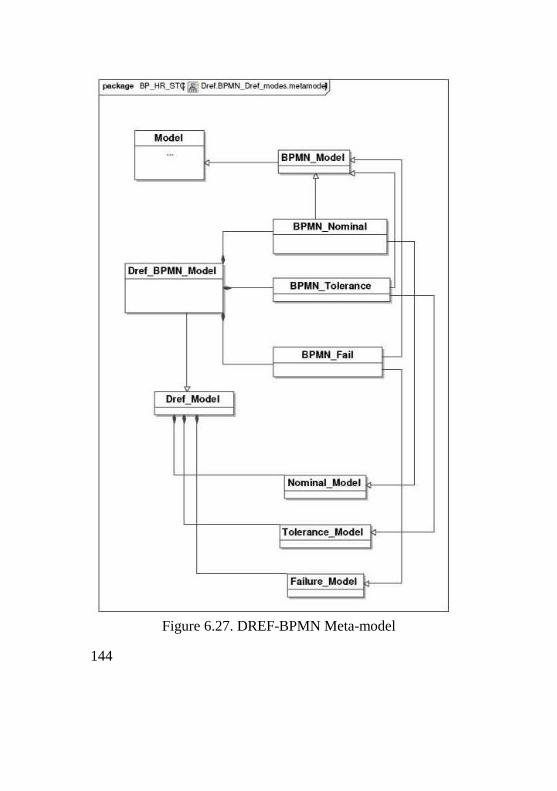
144

Figure 6.27. DREF-BPMN Meta-model

145

The Nominal Mode

Let us consider a simple Human Resources (HR) Department. The

HR department has one business process which manages short term

contracts (STC) for specific missions. Let us have the following

informal requirements description: HR department has as a goal to

process the STC recruitments for the different services of the company.

Each time a service has a position to fill, he provides the position

description to the HR such that HR can start the process. HR publishes

the position using external diffusion (such as journals, web, national

recruitment services). Applications are received until the position is

closed i.e. when at least 2 applicants applied. All applicants are

interviewed and then the HR selects the best candidate. The contract is

signed with the selected candidate. Finally, company service and

unselected applicants are notified.

According to the meta-model, this BPMN model for the nominal

mode is made of a process model (cf. Figure 6.28), a concept model (cf.

Figure 6.29 and 6.30) and a constraint model (cf. Figure 6.31). In

Figure 6.28, the BPMN model of this STC contract BP of the HR

department is we provided. This BP model should be considered as the

process that the HR must apply in case of STC management.

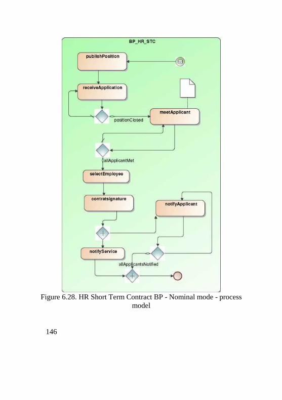
146

Figure 6.28. HR Short Term Contract BP - Nominal mode - process

model

147

According to the meta-model (Figure 10), the activities are related

to data which are modelled in the concept model (Figure 6.29). This

data model more precisely describes the concepts, which are mentioned

in the informal requirements (of course this should be performed in an

iterative process involving all the concerned stakeholders).

In order to specify more precisely the activities of the BP let us

provide for each of its activities (listed in the interface view of Figure

6.30) a pre/post axiomatic specification using OCL [90]. An example of

such a specification is provided in Figure 6.31. In this specification, the

pre-condition of the meetApplicant activity indicates that the HR

department has not previously interviewed the candidate (if this is not

the case, the outcome of this activity is not known and the fault will not

be attributed to the HR). The post-condition, indicates that the HR

registers the fact that this applicant has been interviewed.

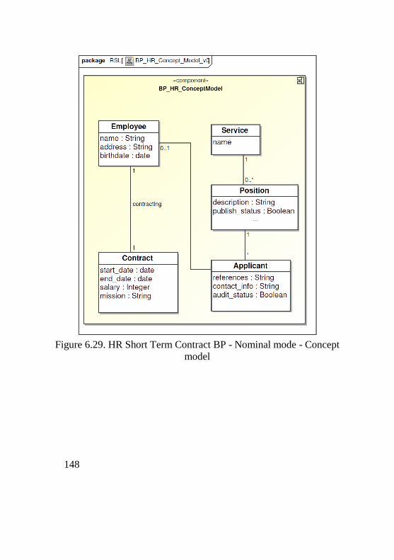
148

Figure 6.29. HR Short Term Contract BP - Nominal mode - Concept

model

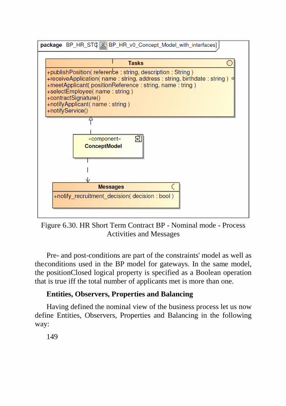
149

Figure 6.30. HR Short Term Contract BP - Nominal mode - Process

Activities and Messages

Pre- and post-conditions are part of the constraints' model as well as

the conditions used in the BP model for gateways. In the same model,

the positionClosed logical property is specified as a Boolean operation

that is true iff the total number of applicants met is more than one.

Entities, Observers, Properties and Balancing

Having defined the nominal view of the business process let us now

define Entities, Observers, Properties and Balancing in the following

way:

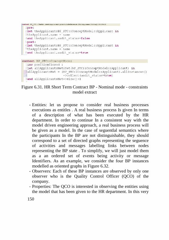
150

Figure 6.31. HR Short Term Contract BP - Nominal mode - constraints

model extract

- Entities: let us propose to consider real business processes

executions as entitles . A real business process Is given In terms

of a description of what has been executed by the HR

department. In order to continue In a consistent way with the

model driven engineering approach, a real business process will

be given as a model. In the case of seguentlal semantics where

the participants In the BP are not distinguishable, they should

correspond to a set of directed graphs representing the seguence

of activities and messages labelling links between nodes

representing the BP state . To simplify, we will just model them

as a an ordered set of events being activity or message

Identifiers. As an example, we consider the four BP instances

modelled as oriented graphs in Figure 6.32.

- Observers: Each of these BP instances are observed by only one

observer who is the Quality Control Officer (QCO) of the

company.

- Properties: The QCO is interested in observing the entities using

the model that has been given to the HR department. In this very

151

simple case, we consider that the property is provided by the BP

Process Models' view (the conjunction of the models provided in

Figures 6.28-6.31).

- Balancing: In this very simple illustration we have one observer

and one property. We thus have a default balancing such that the

weight of the observer and the property are egual to 1.

Evolution and Observation axis

Let us define two axes for the purpose of illustrating the DREF

framework in model driven engineering and development processes:

- An evolution axis (ev) has two indexes (1 and 2) representing

one evolution step of the HR service. While in the first one the

HR employee activities would be evaluated according to a non

fault-tolerant business process (modelled in Figure 6.43). The

second version of the HR department introduces a tolerance

margin (described in Figure 6.34).

- An observation axis (obs) with four indexes (1 to 4) to denotes

the 4 observation points is shown in Figure 6.32. They represent

four completed recruitment processes executed by the actual HR

Service.

-

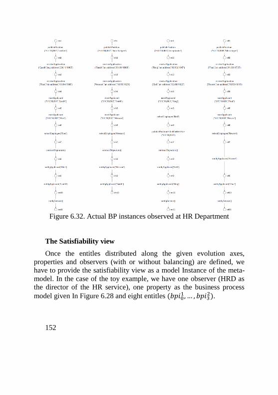
152

Figure 6.32. Actual BP instances observed at HR Department

The Satisfiability view

Once the entitles distributed along the given evolution axes,

properties and observers (with or without balancing) are defined, we

have to provide the satisfiability view as a model Instance of the meta-

model. In the case of the toy example, we have one observer (HRD as

the director of the HR service), one property as the business process

model given In Figure 6.28 and eight entitles (𝑏𝑝𝑖01, … , 𝑏𝑝𝑖3

2).

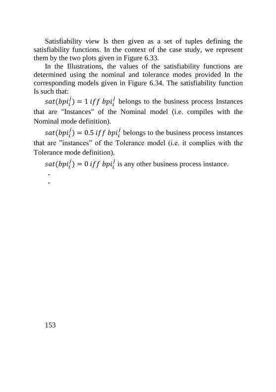
153

Satisfiability view Is then given as a set of tuples defining the

satisfiability functions. In the context of the case study, we represent

them by the two plots given in Figure 6.33.

In the Illustrations, the values of the satisfiability functions are

determined using the nominal and tolerance modes provided In the

corresponding models given in Figure 6.34. The satisfiability function

Is such that:

𝑠𝑎𝑡(𝑏𝑝𝑖𝑖𝑗) = 1 𝑖𝑓𝑓 𝑏𝑝𝑖𝑖

𝑗 belongs to the business process Instances

that are "Instances" of the Nominal model (i.e. compiles with the

Nominal mode definition).

𝑠𝑎𝑡(𝑏𝑝𝑖𝑖𝑗) = 0.5 𝑖𝑓𝑓 𝑏𝑝𝑖𝑖

𝑗 belongs to the business process instances

that are ”instances” of the Tolerance model (i.e. it complies with the

Tolerance mode definition).

𝑠𝑎𝑡(𝑏𝑝𝑖𝑖𝑗) = 0 𝑖𝑓𝑓 𝑏𝑝𝑖𝑖

𝑗 is any other business process instance.

- -

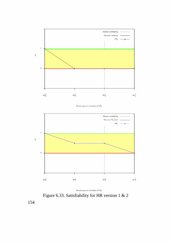
154

Figure 6.33. Satisfiability for HR version 1 & 2

155

In Figure 6.5 the Failure view(s), which is used here only to model

a subset of the business process instances for which the satisfiability

function returns a failure (below the tolerance margin), is included.

Depending on the DREF extension targeted, either this view could be

considered as fully characterising the failures or only a subset. In the

first case, any business process instance not in the nominal, tolerance,

or failure sets should either not be in the definition domain of sat or the

sat value should be ⊥. In the second case, the view should be used to

document a subset of failing business process instances.

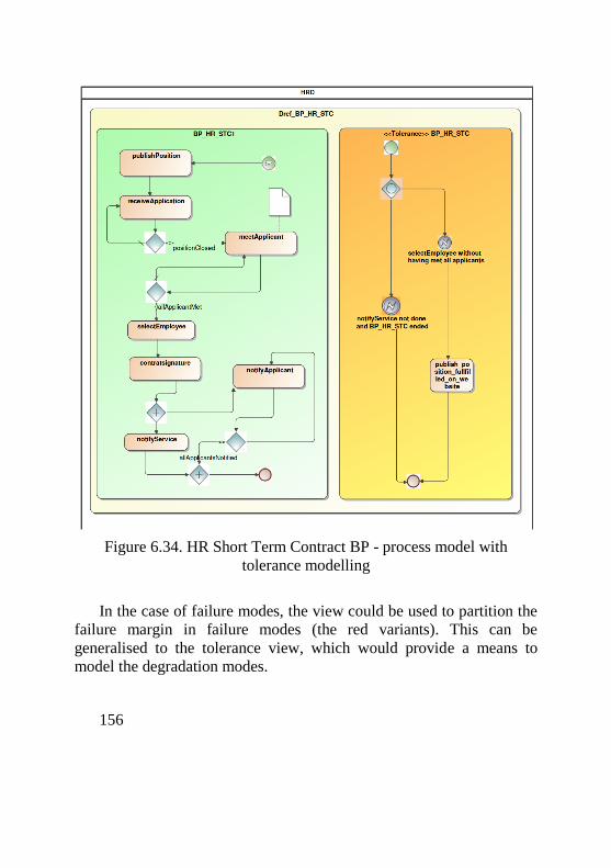
156

Figure 6.34. HR Short Term Contract BP - process model with

tolerance modelling

In the case of failure modes, the view could be used to partition the

failure margin in failure modes (the red variants). This can be

generalised to the tolerance view, which would provide a means to

model the degradation modes.

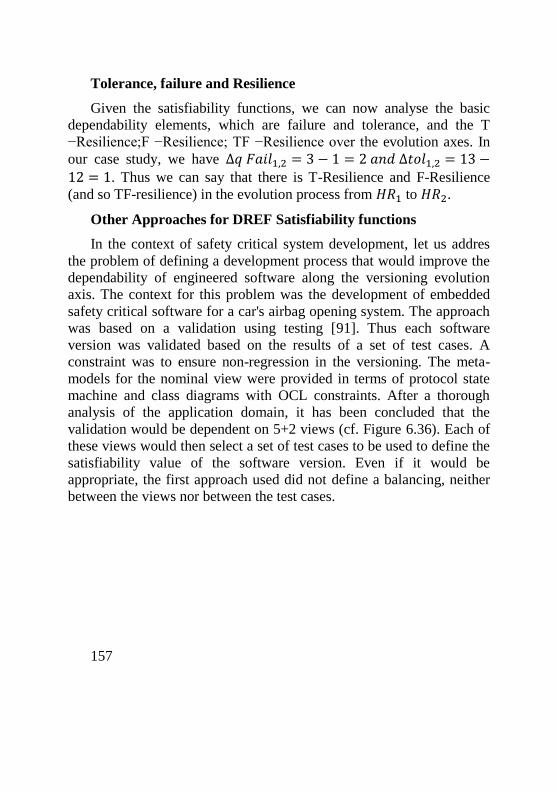
157

Tolerance, failure and Resilience

Given the satisfiability functions, we can now analyse the basic

dependability elements, which are failure and tolerance, and the T

−Resilience;F −Resilience; TF −Resilience over the evolution axes. In

our case study, we have ∆𝑞 𝐹𝑎𝑖𝑙1,2 = 3 − 1 = 2 𝑎𝑛𝑑 ∆𝑡𝑜𝑙1,2 = 13 −12 = 1. Thus we can say that there is T-Resilience and F-Resilience

(and so TF-resilience) in the evolution process from 𝐻𝑅1 to 𝐻𝑅2.

Other Approaches for DREF Satisfiability functions

In the context of safety critical system development, let us addres

the problem of defining a development process that would improve the

dependability of engineered software along the versioning evolution

axis. The context for this problem was the development of embedded

safety critical software for a car's airbag opening system. The approach

was based on a validation using testing [91]. Thus each software

version was validated based on the results of a set of test cases. A

constraint was to ensure non-regression in the versioning. The meta-

models for the nominal view were provided in terms of protocol state

machine and class diagrams with OCL constraints. After a thorough

analysis of the application domain, it has been concluded that the

validation would be dependent on 5+2 views (cf. Figure 6.36). Each of

these views would then select a set of test cases to be used to define the

satisfiability value of the software version. Even if it would be

appropriate, the first approach used did not define a balancing, neither

between the views nor between the test cases.

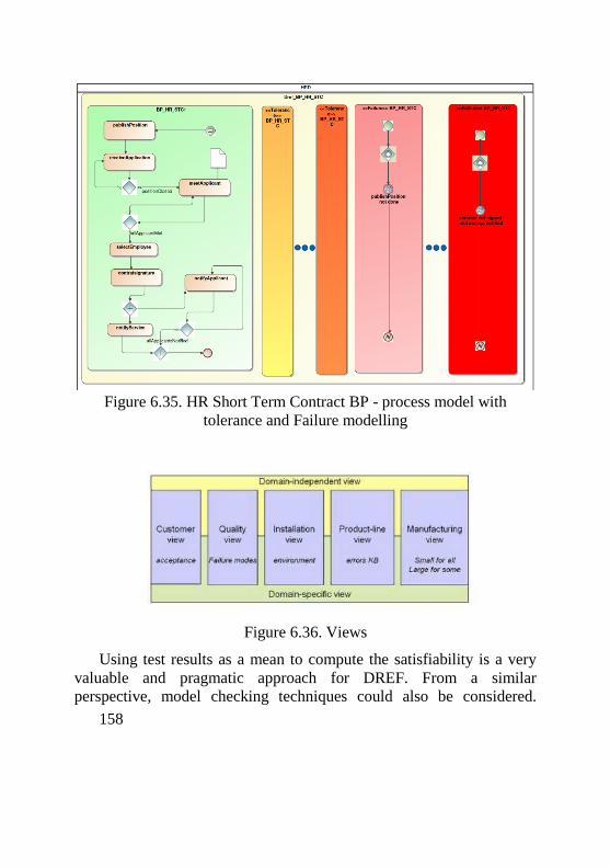
158

Figure 6.35. HR Short Term Contract BP - process model with

tolerance and Failure modelling

Figure 6.36. Views

Using test results as a mean to compute the satisfiability is a very

valuable and pragmatic approach for DREF. From a similar

perspective, model checking techniques could also be considered.

159

Practical use of the DREF framework is currently limited to the field of

DSL development (as illustrated by the case study). Currently

additional experiments to better assess the framework are conducted.

One experiment in the field of operational resilience [92] uses entities

as algebraic Petri net models [93], properties as invariants regarding

places in the APN, and satisfiability as logical functions computed

using the model checker AlPiNA [94]. A second experiment was

performed in the context of architecture description languages [95]. The

aim was to improve the AADL modeling language with the DREF

concepts, thus engineering an architecture description language for

resilient architectures. Those experiments provide a practical

assessment of the usefulness of the approach presented in this article for

the specific aims targeted.

Conclusion

In this section, an initial version of a formal framework DREF that

precisely defines the fundamentals concepts used to define

dependability and resilience of ICT systems is introduced. This

framework has been defined using set theory at a chosen abstraction

level in order to cover the current advances in the terminology of

dependable and resilient systems engineering. The proposed framework

has been designed to be useful for ICT system model driven

engineering. To this extent, a meta-model has been proposed for the

framework and a validation of the approach using the DREF framework

for modelling language engineering has been provided.

Advancement questions

1. What is the KAOS?

2. What does KAOS specification language provide?

3. What we should do to formally express these security goals?

4. What we need to do for applying the generic security model to

a system?

160

5. What is the difference between the OR and AND-refinement?

6. What is the FADSE framework?

7. What are the main limitations of the semi-formal approaches to

security engineering?

8. What is the difference between the dependability and

resilience?

9. What is the model driven engineering?

10. What is main purpose of the DREF?

REFERENCES

1. Hassan R. Formal Analysis and Design for Engineering

Security / R. Hassan // PhD thesis. – Blacksburg, Virginia. -

2009. - p. 235.

2. A. van Lamsweerde Handling Obstacles in Goal-Oriented

Requirements Engineering / A. van Lamsweerde, E. Letier //

IEEE Transactions on Software Engineering, Special Issue on

Exception Handling. – 2000. - Vol. 26, No. 10. – pp. 978-1005.

3. Lamsweerde, A. Building Formal Requirements Models for

Reliable Software / A.Lamsweerde // Proceedings of the 6th

Ade- Europe International Conference Leuven on Reliable

Software Technologies.-2001.- pg. 1-20.

4. A. van Lamsweerde Elaborating Security Requirements by

Construction of Intentional Anti-Models / A.Lamsweerde//

Proc. ICSE’04: 26th Intl. Conf. on Software Engineering.-2004.

5. Landtsheeer, R. Reasoning about Confidentiality at

Requirements Engineering Time / R.Landtsheeer,

A.Lamsweerde // Proceedings of the 19h European Software

Engineering Conference held jointly with 13th ACM SIGSOFT

161

International Symposium on Foundations of Software

Engineering. - 2005.- pg. 41-49.

6. Ponsard, C. Early Verification and Validation of Mission

Critical Systems / C Ponsard,., et. al. // Proceedings of the 9th

International Workshop on Formal Methods for Industrial

Critical systems (FMICS).- 2004.

7. Letier, E. Agent-Based Tactics for Goal-Oriented Requirements

Elaboration / E.Letier, A.Lamsweerde, // Proceedings of the

24th International Conference on Software Engineering.- 2002.-

pg. 83-93,.

8. Letier, E. Deriving Operational Software Specifications from

System Goals / E.Letier, , A.Lamsweerde, // ACM SIGSOFT

Software Engineering Notes.-Vol. 27, Issue 6.-pg. 119-128,

2002.

9. Fontaine, P.J. Goal-Oriented Elaboration of Security

Requirements, M.S. Thesis / P.J Fontaine // Dept. Computing

Science : University of Louvain, 2001.

10. Lamsweerde, A. Goal-Oriented Requirements Engineering: A

Roundtrip from Research to Practice / Lamsweerde, A. //

Proceedings of the 12th IEEE International Requirements

Engineering Conference (RE’04).- 2004.

11. Darimont, R. Formal Refinement Patterns for Goal-Driven

Requirements Elaboration / R.Darimont, A. van Lamsweerde //

Proc. Fourth ACM SIGSOFT Symp. Foundations of Software

Eng..- 1996.-pp. 179-190.

12. Letier, E. Reasoning about Partial Goal Satisfaction for

Requirements and Design Engineering / E.Letier,

A.Lamsweerde, // ACM SIGSOFT Software Engineering

Notes.-2004.- Vol. 29, Issue 6.- pg. 53-62.

162

13. Lamsweerde, A. Leaving Inconsistency / A.Lamsweerde, et. al.

// Proceedings of the ICSE’97 Workshop on “Living with

Inconsistency".-1997.

14. van Lamsweerde A. Goal- Directed Elaboration of

Requirements for a Meeting Scheduler: Problems and Lessons

Learned / A. van Lamsweerde, R.Darimont, P.Massonet //

Proc. Second Int'l Symp. Requirements Eng. (RE '95).- 1995.

15. Landtsheer, R. Reasoning about Confidentiality at

Requirements Engineering Time / R.Landtsheer, A.Van

Lamsweerde, // Proceedings of the 10th European software

Engineering Conference.-2005.- pg. 41-49.

16. Letier, E. High Assurance Requires Goal Orientation / E.Letier,

A. Van Lamsweerde // International Workshop Requirements

for High Assurance Systems.- 2004.

17. Fontaine, P.J., Goal-Oriented Elaboration of Security

Requirements, M.S. Thesis/ P.J.Fontaine, // Dept. Computing

Science: University of Louvain.-2001.

18. J. Viega Building Secure Software: How to Avoid Security

Problems the Right Way / J. Viega, G. McGraw // Addison-

Wesley.- 2001.

19. Wing A Symbiotic Relationship Between Formal Methods and

Security / Wing, Jeannette // Proceedings of Computer Security,

Dependability and Assurance: From Needs to solutions.-1998.-

pg. 26-38.

20. Beeck A. Formal Requirements Engineering Method for

Specification / Beeck, V.Michael, Margaria, Tiziana, Steffen,

Bernhard, // Synthesis, and Verification, in Proceedings of the

8th conference on Software Engineering Environments.-1997.-

pg. 131-144.

163

21. B. Nuseibeh A Framework for Expressing the Relationships

Between Multiple Views in Requirements Specifications / B.

Nuseibeh, J. Kramer, A. Finkelstein // IEEE Transactions on

Software Engineering.-1994.-Vol. 20 No. 10.-pg.760-773.

22. Van Lamsweerde, A. Formal Specification: a Roadmap / A.Van

Lamsweerde, A. Finkelstein // Proceedings of the Future of

Software Engineering.- ACM Press, 2000.

23. J. Mylopoulos From Object-Oriented to Goal-Oriented

Requirements Analysis / J. Mylopoulos, L. Chung, E. Yu //

Communications of the ACM.-1999.- №42(1 ):31-37.

24. Y.Yu From stakeholder goals to high-variability software

design. Tech. Rep. CSRG-509 / Y.Yu, et. al..-Canada,Ontario:

University of Toronto, 2005.

25. William Heaven A UML profile to support requirements

engineering with KAOS / William Heaven and Anthony

Finkelstein // IEE Proceedings: Software.-2004.- Vol.151, Issue

No. 1, pg. 10-27.

26. L. Jiang Incorporating Goal Analysis in Database Design: A

Case Study from Biological Data Management. / L. Jiang, T.

Topaloglou, A. Borgida, J. Mylopoulos // RE’.-2006.-pg. 196-

204.

27. Bowen, J.Application of Formal Methods / J.Bowen,

M.Hinchey // Prentice Hall.- 1995

28. Clarke Formal Methods: State of the Art and Future Directions

/ Clarke, Edmund, J.Wing, et. al. // ACM Computing Surveys.-

1996.- Vol. 28, No. 4.

29. The Common Criteria for Information Technology Security

Evaluation (CC)[Electronic resourse].- Access

mode:http://www.commoncriteriaportal.org/

164

30. Stepney An Electronic Purse Specification, Refinement, and

Proof / Stepney, Susan, Cooper, et. al. // Programming

Research Group: Oxford University Computing Labarotory.-

2000.

31. Sabatier, D. The Use of the B Formal Method for the Design

and the Validation of the Transaction Mechanism for Smart

Card Applications / D.Sabatier, L.Pierre// In the 17th

Proceedings of Formal Methods in System Design.-2000.- pg.

245-¬272.

32. McDermott J. Using abuse case models for security

requirements analysis / J.McDermott, C.Fox // Proceedings of

the 15th annual computer security applications conference

(ACSAC’99),Phoenix, Arizona.-1999.-№1.

33. G. Sindre Eliciting Security Requirements by Misuse Cases / G.

Sindre, A.L. Opdahl // Proc. TOOLS Pacific’2000 - Techn. of

Object-Oriented Languages and Systems.-2000.- pg.120-131.

34. Firesmith Security Use Cases[Electronic resourse] / Firesmith,

G.Donald // Journal of Object Technology (JOT).-2003.-issue

5.- Access mode:http://www.jot.fm/issues/issue 2003

05/column6

35. L. Liu Security and Privacy Requirements Analysis within a

Social Setting / L. Liu, E. Yu, J. Mylopoulos // Proc.RE’03-

Intl. Conf. Requirements Engineering.- 2003.-pg.151-161.

36. L. Chung Nonfunctional requirements in software engineering.

/ L. Chung, B. Nixon, E. Yu, J. Mylopoulos.- Boston:Kluwer

Academic,2000.

37. Yu, E. Why Agent-Oriented Requirements Engineering / E.Yu

// Proc. of the 3rd Int. Workshop on Requirements Engineering:

Foundations for Software Quality, Barcelona, Catalonia. E.

165

Dubois, A.L. Opdahl, K. Pohl, eds. Presses Universitaires de

Namur.-1997.

38. Nakagawa, H. Formal Specification Generator for KAOS /

H.Nakagawa, K.Taguchi, S.Honiden // Proceedings of The

International Conference on Automated Software Engineering

(ASE’07).-2007.

39. Brandozzi, M. Transforming Goal Oriented Requirement

Specifications into Architectural Prescriptions /

M.BRANDOZZI, D. E. PERRY.- Toronto, Canada:First

International Workshop from Software Requirements to

Architectures (STRAW'01).

40. Van Lamsweerde, A. From System Goals to Software

Architecture. / A.Van Lamsweerde // in Formal Methods for

Software Architectures. M. Bernardo and P. Inverardi,

Springer-Verlag.-2003.-pg.25-43.

41. Liu, L. From Requirements to Architectural Design - Using

Goals and Scenarios./L.Liu, E.Yu // ICSE- 2001 Workshop:

From Software Requirements to Architectures (STRAW2001).-

2001.- pp. 22-30.

42. J. Mylopoulos UML for agent-oriented software

development:The Tropos proposal / J. Mylopoulos, M. Kolp,

J. Castro // Proc. of the 4th Int. Conf. on the Unified Modeling

Language UML.-2001

43. R. G. Dromey From requirements to design: Formalizing the

key steps / R. G. Dromey // International Conference on

Software Engineering and Formal Methods: The University of

Queensland School of Information Technology and Electrical

Engineering,2003.- pp. 2.13.

166

44. M.G. Hinchey Requirements to Design to Code: Towards a

Fully Formal Approach to Automatic Code Generation / J.L.

Rash, C.A. Rouff // NASA Technical Report.-2005.

45. Hoss Ontological Approach to Improving Design Quality /

Hoss, M.Allyson, Carver, L.Doris // in Proceeding of IEEE

Aerospace Conference.-2006.- pg.12.

46. J. Liu Linking UML models of design and requirement / J. Liu,

Z. Liu, J. He, X. Li.-Melbourne, Australia:IEEE Computer

Society. 82, 2004.

47. X. Li Formal and use-case driven requirement analysis in UML

/ X. Li, Z. Liu, J. He.-Illinois, USA: IEEE Computer

Society,2001

48. Z. Liu A relational model for formal object-oriented

requirement analysis in UML / J. He, X. Li, Y. Chen //

Lecture Notes in Computer Science 2885. Springer.- 2003.

49. Hung Ledang Formalizing UML behavioral diagrams with B.

In Tenth OOPSLA Workshop on Behavioral Semantics : Back

to Basics / Hung Ledang and Jeanine Souquieres.- Tampa Bay,

Florida, USA, 2001.

50. Hung Ledang MODELING CLASS OPERATIONS IN B:

application to UML behavioral diagrams. / Hung Ledang,

Jeanine Souquieres.- Loews Coronado Bay, San Diego, USA,:

IEEE Computer Society,2001.

51. Hung Ledang Integration of UML Views Using B Notation /

Hung Ledang, Jeanine Souquieres // In proceedings of

WITUML02,Spain.-2002.

52. Blackburn, M. Removing Requirements Defects and

Automating Test / M.Blackburn, R.Busser, A.Nauman, //

Software Productivity Consortium.-2001.

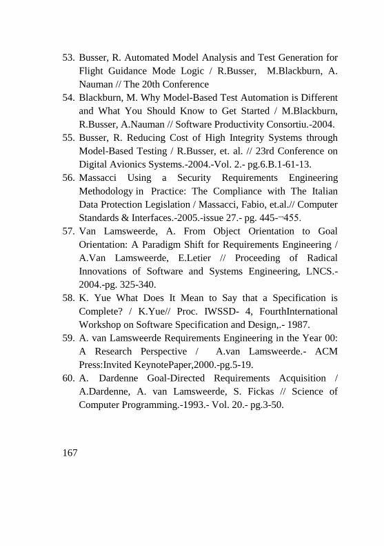
167

53. Busser, R. Automated Model Analysis and Test Generation for

Flight Guidance Mode Logic / R.Busser, M.Blackburn, A.

Nauman // The 20th Conference

54. Blackburn, M. Why Model-Based Test Automation is Different

and What You Should Know to Get Started / M.Blackburn,

R.Busser, A.Nauman // Software Productivity Consortiu.-2004.

55. Busser, R. Reducing Cost of High Integrity Systems through

Model-Based Testing / R.Busser, et. al. // 23rd Conference on

Digital Avionics Systems.-2004.-Vol. 2.- pg.6.B.1-61-13.

56. Massacci Using a Security Requirements Engineering

Methodology in Practice: The Compliance with The Italian

Data Protection Legislation / Massacci, Fabio, et.al.// Computer

Standards & Interfaces.-2005.-issue 27.- pg. 445-¬455.

57. Van Lamsweerde, A. From Object Orientation to Goal

Orientation: A Paradigm Shift for Requirements Engineering /

A.Van Lamsweerde, E.Letier // Proceeding of Radical

Innovations of Software and Systems Engineering, LNCS.-

2004.-pg. 325-340.

58. K. Yue What Does It Mean to Say that a Specification is

Complete? / K.Yue// Proc. IWSSD- 4, FourthInternational

Workshop on Software Specification and Design,.- 1987.

59. A. van Lamsweerde Requirements Engineering in the Year 00:

A Research Perspective / A.van Lamsweerde.- ACM

Press:Invited KeynotePaper,2000.-pg.5-19.

60. A. Dardenne Goal-Directed Requirements Acquisition /

A.Dardenne, A. van Lamsweerde, S. Fickas // Science of

Computer Programming.-1993.- Vol. 20.- pg.3-50.

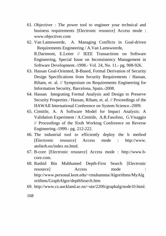
168

61. Objectiver : The power tool to engineer your technical and

business requirements [Electronic resource] Access mode :

www.objectiver.com

62. Van Lamsweerde, A. Managing Conflicts in Goal-driven

Requirements Engineering / A.Van Lamsweerde,

R.Darimont, E.Letier // IEEE Transactions on Software

Engineering, Special Issue on Inconsistency Management in

Software Development.-1998.- Vol. 24, No. 11.- pg. 908-926.

63. Hassan Goal-Oriented, B-Based, Formal Derivation of Security

Design Specifications from Security Requirements / Hassan,

Riham, et. al. // Symposium on Requirements Engineering for

Information Security, Barcelona, Spain.-2008.

64. Hassan Integrating Formal Analysis and Design to Preserve

Security Properties / Hassan, Riham, et. al. // Proceedings of the

HAWAII International Conference on System Science.-2009.

65. Cimitile, A. A Software Model for Impact Analysis: A

Validation Experiment / A.Cimitile, A.R.Fasolino, G.Visaggio

// Proceedings of the Sixth Working Conference on Reverse

Engineering.-1999.- pg. 212-222.

66. The industrial tool to efficiently deploy the b method

[Electronic resource] Access mode : http://www.

atelierb.eu/index en.html.

67. B-core [Electronic resource] Access mode : http://www.b-

core.com.

68. Rashid Bin Muhhamed Depth-First Search [Electronic

resource] Access mode :

http://www.personal.kent.edu/~rmuhamma/Algorithms/MyAlg

orithms/GraphAlgor/depthSearch.htm

69. http://www.cs.auckland.ac.nz/~ute/220ft/graphalg/node10.html.

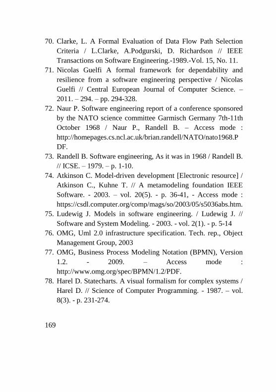
169

70. Clarke, L. A Formal Evaluation of Data Flow Path Selection

Criteria / L.Clarke, A.Podgurski, D. Richardson // IEEE

Transactions on Software Engineering.-1989.-Vol. 15, No. 11.

71. Nicolas Guelfi A formal framework for dependability and

resilience from a software engineering perspective / Nicolas

Guelfi // Central European Journal of Computer Science. –

2011. – 294. – pp. 294-328.

72. Naur P. Software engineering report of a conference sponsored

by the NATO science committee Garmisch Germany 7th-11th

October 1968 / Naur P., Randell B. – Access mode :

http://homepages.cs.ncl.ac.uk/brian.randell/NATO/nato1968.P

DF.

73. Randell B. Software engineering, As it was in 1968 / Randell B.

// ICSE. – 1979. – p. 1-10.

74. Atkinson C. Model-driven development [Electronic resource] /

Atkinson C., Kuhne T. // A metamodeling foundation IEEE

Software. - 2003. – vol. 20(5). - p. 36-41, - Access mode :

https://csdl.computer.org/comp/mags/so/2003/05/s5036abs.htm.

75. Ludewig J. Models in software engineering. / Ludewig J. //

Software and System Modeling. - 2003. - vol. 2(1). - p. 5-14

76. OMG, Uml 2.0 infrastructure specification. Tech. rep., Object

Management Group, 2003

77. OMG, Business Process Modeling Notation (BPMN), Version

1.2. - 2009. – Access mode :

http://www.omg.org/spec/BPMN/1.2/PDF.

78. Harel D. Statecharts. A visual formalism for complex systems /

Harel D. // Science of Computer Programming. - 1987. – vol.

8(3). - p. 231-274.

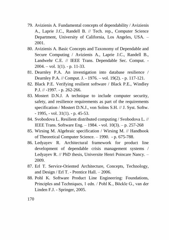
170

79. Avizienis A. Fundamental concepts of dependability / Avizienis

A., Laprie J.C., Randell B. // Tech. rep., Computer Science

Department, University of California, Los Angeles, USA. –

2001.

80. Avizienis A. Basic Concepts and Taxonomy of Dependable and

Secure Computing / Avizienis A., Laprie J.C., Randell B.,

Landwehr C.E. // IEEE Trans. Dependable Sec. Comput. -

2004. – vol. 1(1). - p. 11-33.

81. Dearnley P.A. An investigation into database resilience /

Dearnley P.A. // Comput. J. - 1976. – vol. 19(2). - p. 117-121.

82. Black P.E. Verifying resilient software / Black P.E., Windley

P.J. // -1997. - p. 262-266.

83. Mostert D.N.J. A technique to include computer security,

safety, and resilience requirements as part of the requirements

specification / Mostert D.N.J., von Solms S.H. // J. Syst. Softw.

- 1995, - vol. 31(1). - p. 45-53.

84. Svobodova L. Resilient distributed computing / Svobodova L. //

IEEE Trans. Software Eng. – 1984. - vol. 10(3). – p. 257-268

85. Wirsing M. Algebraic specification / Wirsing M. // Handbook

of Theoretical Computer Science. – 1990. - p. 675-788.

86. Ledyayev R. Architectural framework for product line

development of dependable crisis management systems /

Ledyayev R. // PhD thesis, Universite Henri Poincare Nancy. –

2009.

87. Erl T. Service-Oriented Architecture, Concepts, Technology,

and Design / Erl T. - Prentice Hall. – 2006.

88. Pohl K. Software Product Line Engineering: Foundations,

Principles and Techniques, 1 edn. / Pohl K., Böckle G., van der

Linden F.J. - Springer, 2005.

171

89. Budinsky F. Eclipse Modeling Framework / Budinsky F.,

Brodsky S.A., Merks E. - Pearson Education. – 2003.

90. OMG, Ocl 2.0 specification. Tech. rep., Object Management

Group. - 2005

91. Guelfi N. Selection, evaluation and generation of test cases in

an industrial setting, a process and a tool / Guelfi N., Ries B. //

Testing, Academic & Industrial Conference, 47-51, IEEE,

Windsor, UK. – 2008.

92. Lúcio L. A precise definition of operational resilience / Lúcio

L., Guelfi N. // Tech. Rep. TR-LASSY-11-02, Laboratory for

Advanced Software Systems, University of Luxembourg. –

2011.

93. Reisig W. Petri nets and algebraic specifications / Reisig W. //

Theor. Comput. Sci. – 1991. - p. 1-34.

94. A symbolic model checker / Buchs D., Hostettler S., Marechal

A., Risoldi M., Alpina // Lecture Notes in Computer Science.

Springer. - 2010. - Vol. 6128.

95. Saidane A. Dref resiliency and security aspects in the sae

architecture analysis and design language (aadl) / Saidane A. //

Tech. Rep. TR-LASSY-10-07, University of Luxembourg. -

2010.

172

7 FORMAL METHODS FOR ARCHITECTING SECURE

SOFTWARE SYSTEMS

Content of the CHAPTER 7

7.1 Semi-formal Security Modelling and Analysis Approaches ... 175

7.2 MAC-UML Framework .......................................................... 176

7.3 SecureUML ............................................................................. 178

7.4 Separating Modelling of Application and Security Concerns . 180

7.5 Formal Security Modelling and Analysis Approaches ............ 182

7.6 Integrated Semi-formal and Formal Modelling and Analysis

Approaches .................................................................................... 188

7.7 Aspect-Oriented Security Modelling and Analysis Approaches191

7.8 Discussion ................................................................................ 195

173

Introduction

Systematical engineering security into software applications is an

important and difficult problem [1, 2, 3, 4] The importance of the

problem can be seen from the number of security incidents reported to

the Computer Emergency Readiness Team Coordination Center

(CERT/CC) and their associated costs.The CERT/CC data from 2003

reports 137,529 incidents; the cost of electronic crimes is reported at

666 million dollars [5]. Most of these incidents, which can involve from

one to thousands of sites, result from software vulnerabilities. The

CERT/CC data indicate the number of these incidents continues to rise.

The difficulty of the problem stems from its breadth, as it covers many

areas such as authentication, auditing, authorization, confidentiality,

integrity, and non-repudiation (security standard ISO 7498-2) [6],

where authentication verifies the claimed identity of a user or provider,

auditing ensures that user activity is properly recorded and reviewed,

authorization moderates information use and provision, confidentiality

means information is provided only for proper use as appropriate to the

sensitivity of the information, integrity makes certain that information

is used in ways that allow only necessary changes, and non-repudiation

ensures the identity of a user is irrefutably verified and recorded as

protection against their later denying participation. Each of these can be

further categorized. For example, authentication may include peer

entity authentication and data origin authentication; confidentiality may

include connection confidentiality, connectionless confidentiality,

selective field confidentiality, and traffic flow confidentiality, etc., as

presented in Figure 7.1.

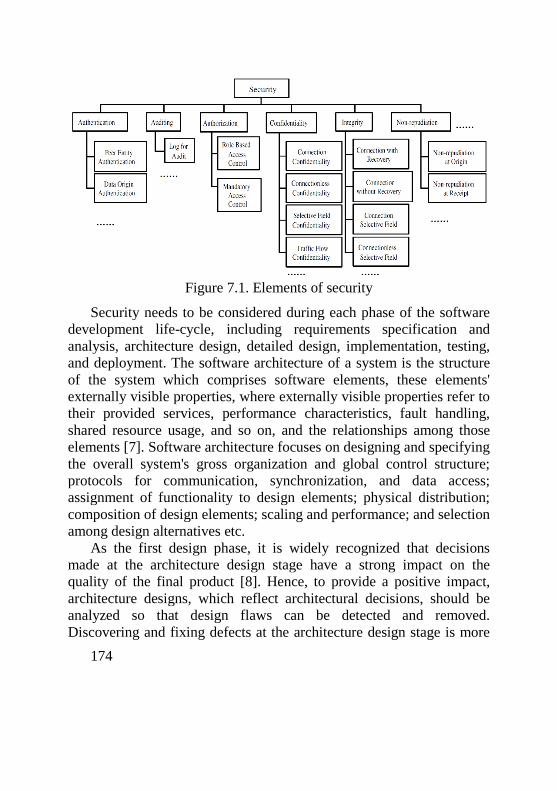
174

Figure 7.1. Elements of security

Security needs to be considered during each phase of the software

development life-cycle, including requirements specification and

analysis, architecture design, detailed design, implementation, testing,

and deployment. The software architecture of a system is the structure

of the system which comprises software elements, these elements'

externally visible properties, where externally visible properties refer to

their provided services, performance characteristics, fault handling,

shared resource usage, and so on, and the relationships among those

elements [7]. Software architecture focuses on designing and specifying

the overall system's gross organization and global control structure;

protocols for communication, synchronization, and data access;

assignment of functionality to design elements; physical distribution;

composition of design elements; scaling and performance; and selection

among design alternatives etc.

As the first design phase, it is widely recognized that decisions

made at the architecture design stage have a strong impact on the

quality of the final product [8]. Hence, to provide a positive impact,

architecture designs, which reflect architectural decisions, should be

analyzed so that design flaws can be detected and removed.

Discovering and fixing defects at the architecture design stage is more

175

cost- and time-effective compared to performing such work after the

system is implemented, as fixing defects at the implementation stage

would necessarily cause the revision and reconstruction of numerous

design, implementation, and testing artifacts. Therefore, the

architectural design and analysis of security properties is a very

important step in the software development lifecycle. The architectural

design of security properties enables the realization of a system's

security non-functional requirements; the analysis of security properties

provides architects with objective results to evaluate design

alternatives.

Recently, numerous approaches have been proposed to support the

modelling and analysis of security properties in software architecture

designs. Here a survey in which the approaches are classified into four

broad categories: semi-formal (i.e., mainly using semi-formal methods

in the approach), formal (i.e., mainly using formal methods in the

approach), integrated semi-formal and formal (i.e., using a combination

of semi-formal and formal methods), and aspect-oriented (i.e., security

non-functional properties are modelled as aspects) approaches are

presented.

7.1 Semi-formal Security Modelling and Analysis Approaches

Unified Modelling Language(UML)[9], a well-known notation, is a

language for specifying, visualizing, constructing, and documenting

designs of software systems. UML provides graphical notations to

express the design of software systems with semi-formal syntax and

semantics, and an associated language, the Object Constraint Language

(OCL), for expressing logic constraints. UML contains two basic

diagram types: structure diagrams and behavior diagrams. Structure

diagrams depict the static structure of the elements in the system,

including class, composite structure, component, deployment, object,

and package diagrams. Behavior diagrams depict the dynamic behavior

of the elements in the system, including activity, statechart, use case,

communication, interaction overview, sequence, and timing diagrams.

176

UML semantics are defined using a meta-model that is described in a

semi-formal manner using three views: the abstract syntax, well-

formedness rules, and modelling element semantics. The abstract

syntax is provided as a model described in a subset of UML, consisting

of a UML class diagram and a supporting natural language description.

The well- formedness rules are provided using the OCL and natural

language (i.e., English). The UML meta-model is defined as one of the

layers of a four-layer meta-modelling architecture, which includes

meta-metamodel, meta-model, model, and user objects. This section

presents several approaches, which use UML to model and analyze

security non-functional properties.

7.2 MAC-UML Framework

The MAC-UML Framework [10] addresses the issue of

incorporating Mandatory Access Control (MAC) into UML design

artifacts, including use case, class, and sequence diagrams. The

approach focuses on providing support for the definition of clearances

and classifications for relevant UML elements.

In this section the concept of security assurance rules for a UML

design is presented. The basis of such security assurance rules is that

UML use case diagrams, class diagrams, and sequence diagrams are

abstracted into a set of UML elements. For example, there is a UML

use case set UC = {uc1, uc2 ...}, UML actor set AC = |ac1, ac2 ...}, UML

class set C = {c1,c2 ...}, and UML method set M = {m1,m2 ...}. Each

UML element is assigned a clearance (CLR) or classification (CLS)

from the partially ordered set ^ = {± = o1,a2 ...,<rs} where the order

relation a* < oj(i < j) means the security level oj has a higher security

concern than that of a*. Notations ac.CLR, uc.CLS, c.CLSmin,

c.CLSmax and m.CLS represent the CLR of actor ac, the CLS of use

case uc, the min and max CLS of class c, and the CLS of method m,

respectively. Then, three tiers of MAC security assurance rules are

defined to assess the question of how to attain security in a design. Tier

1 security assurance rules represent the creation of use case diagrams

with actors, use cases, actor-use case associations, actor and use case

177

inheritance, and use case inclusion and extension relationships. For

example, one of these security assurance rules can be interpreted as:

For every actor acm that is associated with the use case uc* (as a

behavior of the application), the CLR of the actor acm must dominate

the CLS of the use case uc*. Formally, it can be represented as: V actor

acm and use case u c a c m is securely (MAC) associated with uc* ^

acmCLR > ucy.CLS.

Correspondingly, security assurance rules for actor inheritance, use

case inheritance, use case inclusion, and use case extension have also

been defined. Tier 2 security assurance rules emphasis on defining the

classes that are utilized by each use case: for a class c (intended) to be

used in a sequence diagram to serve the goal (i.e., realize the

functionality) of use case uc, the CLS of the uc must dominate the

minimum CLS of c. Tier 3 security assurance rules are a refinement of

Tier 2 security assurance rules to support method calls between the

different entities (use case and objects) in a sequence diagram. Finally,

algorithms are defined for assessing whether a UML design as a whole

satisfies the security assurance rules by conducting a comprehensive

analysis of the entire design.

The security problem addressed in the approach is mandatory

access control (refer to Figure 7.1). The example system used is a

Survey Institution which performs and manages public surveys. In the

system, after the raw data of the survey is collected, staff with different

privileges will manipulate the database, where senior person can add a

survey header into the database, and another staff person (senior or

junior staff) will add questions into that survey, and also have the

ability to categorize questions and add a new question category if

needed. However, there are some special questions that have more

sensitive content, which only senior staff are allowed to perform data

entry. The strength of the approach is that it bridges the gap between

software engineering and an organization's security personnel. With the

enforcement and assessment of three tiers of security assurance rules,

the MAC capability can be incorporated into a UML design, where

access violations through inheritance, inclusion, and extension can be

178

detected. The approach can be applied to systems where MAC is one of

the priority concerns. Such systems can be a distributed system, or an

information system. The limitation of the approach is: since security

assurance rules in the approach are only explored on a subset of UML

diagrams (i.e., use case, class, and sequence diagram), the approach is

only applicable to a system design that uses these three kinds of

diagrams. In addition, security analysis of the approach is based on the

semi-formal UML, where the relationship inheritance, inclusion, and

extension are not formally defined. To obtain more rigorous analysis

results, a formal specification of the system design is desired.

7.3 SecureUML

SecureUML [11] is a modelling language that defines a vocabulary

for annotating UML based models with information relevant to access

control. It is based on the role-based access control model (RBAC),

with additional support for specifying authorization constraints.

SecureUML defines a vocabulary for expressing different aspects of

access control, like roles, role permissions, and user-role assignments.

Due to its general access-control model and extensibility, SecureUML

is well suited for business analysis as well as design models for

different technologies. The structure of the modelling language

conforms to the reference model for model driven systems. Model-

driven software development is an approach where software systems

are defined using models and constructed, at least in part, automatically

from these models. A system can be modelled at different levels of

abstraction or from different perspectives. The syntax of every model is

defined by a meta-model.

The SecureUML meta-model is defined as an extension of the

UML meta-model. The concepts of RBAC are represented directly as

meta-model types, including User, Role and Permission as well as

relations between these types. Instead of defining a dedicated meta-

model type to represent protected sources, every UML model element

is allowed to take the role of a protected resource. Additionally, the

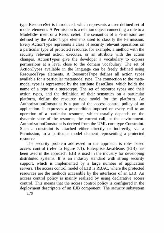
179

type ResourceSet is introduced, which represents a user defined set of

model elements. A Permission is a relation object connecting a role to a

ModelEle- ment or a ResourceSet. The semantics of a Permission are

defined by the ActionType elements used to classify the Permission.

Every ActionType represents a class of security relevant operations on

a particular type of protected resource, for example, a method with the

security relevant action executes, or an attribute with the action

changes. ActionTypes give the developer a vocabulary to express

permissions at a level close to the domain vocabulary. The set of

ActionTypes available in the language can be freely defined using

ResourceType elements. A ResourceType defines all action types

available for a particular metamodel type. The connection to the meta-

model type is represented by the attribute BaseClass, which holds the

name of a type or a stereotype. The set of resource types and their

action types, and the definition of their semantics on a particular

platform, define the resource type model for the platform. An

AuthorizationConstraint is a part of the access control policy of an

application. It expresses a precondition imposed on every call to an

operation of a particular resource, which usually depends on the

dynamic state of the resource, the current call, or the environment.

AuthorizationConstraint is derived from the UML core type Constraint.

Such a constraint is attached either directly or indirectly, via a

Permission, to a particular model element representing a protected

resource.

The security problem addressed in the approach is role- based

access control (refer to Figure 7.1). Enterprise JavaBeans (EJB) has

been used in the approach. EJB is used in the industry for developing

distributed systems. It is an industry standard with strong security

support, which is implemented by a large number of application

servers. The access control model of EJB is RBAC, where the protected

resources are the methods accessible by the interfaces of an EJB. An

access control policy is mainly realized by using declarative access

control. This means that the access control policy is configured in the

deployment descriptors of an EJB component. The security subsystem

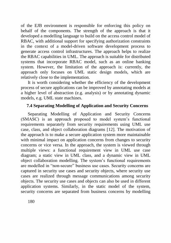
180

of the EJB environment is responsible for enforcing this policy on

behalf of the components. The strength of the approach is that it

developed a modelling language to build on the access control model of

RBAC, with additional support for specifying authorization constraints

in the context of a model-driven software development process to

generate access control infrastructures. The approach helps to realize

the RBAC capabilities in UML. The approach is suitable for distributed

systems that incorporate RBAC model, such as an online banking

system. However, the limitation of the approach is: currently, the

approach only focuses on UML static design models, which are

relatively close to the implementation.

It is worth considering whether the efficiency of the development

process of secure applications can be improved by annotating models at

a higher level of abstraction (e.g. analysis) or by annotating dynamic

models, e.g. UML state machines.

7.4 Separating Modelling of Application and Security Concerns

Separating Modelling of Application and Security Concerns

(SMASC) is an approach proposed to model system’s functional

requirements separately from security requirements using UML use

case, class, and object collaboration diagrams [12]. The motivation of

the approach is to make a secure application system more maintainable

with minimal impact on application concerns from changes to security

concerns or vice versa. In the approach, the system is viewed through

multiple views: a functional requirement view in UML use case

diagram; a static view in UML class, and a dynamic view in UML

object collaboration modelling. The system’s functional requirements

are modelled in “non-secure” business use cases. Security concerns are

captured in security use cases and security objects, where security use

cases are realized through message communications among security

objects. The security use cases and objects can also be used in different

application systems. Similarly, in the static model of the system,

security concerns are separated from business concerns by modelling

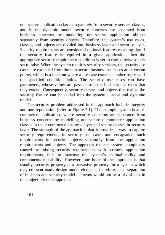
181

non-secure application classes separately from security service classes,

and in the dynamic model, security concerns are separated from

business concerns by modelling non-secure application objects

separately from security objects. Therefore, the system’s use cases,

classes, and objects are divided into business layer and security layer.

Security requirements are considered optional features meaning that if

the security feature is required in a given application, then the

appropriate security requirement condition is set to true, otherwise it is

set to false. When the system requires security services, the security use

cases are extended from the non-secure business use cases at extension

points, which is a location where a use case extends another use case if

the specified condition holds. The security use cases can have

parameters, whose values are passed from the business use cases that

they extend. Consequently, security classes and objects that realize the

security feature can be added into the system’s static and dynamic

model.

The security problem addressed in the approach include integrity

and non-repudiation (refer to Figure 7.1). The example system is an e-

commerce application, where security concerns are separated from

business concerns by modelling non-secure e-commerce application

classes in the e-commerce business layer and secure classes in security

layer. The strength of the approach is that it provides a way to capture

security requirements in security use cases and encapsulate such

requirements in security objects separately from the application

requirements and objects. The approach reduces system complexity

caused by mixing security requirements with business application

requirements, thus to increase the system’s maintainability and

components reusability. However, one issue of the approach is that

usually, security property is a pervasive property for a system which

may crosscut many design model elements; therefore, clear separation

of business and security model elements would not be a trivial task in

this object-oriented approach.

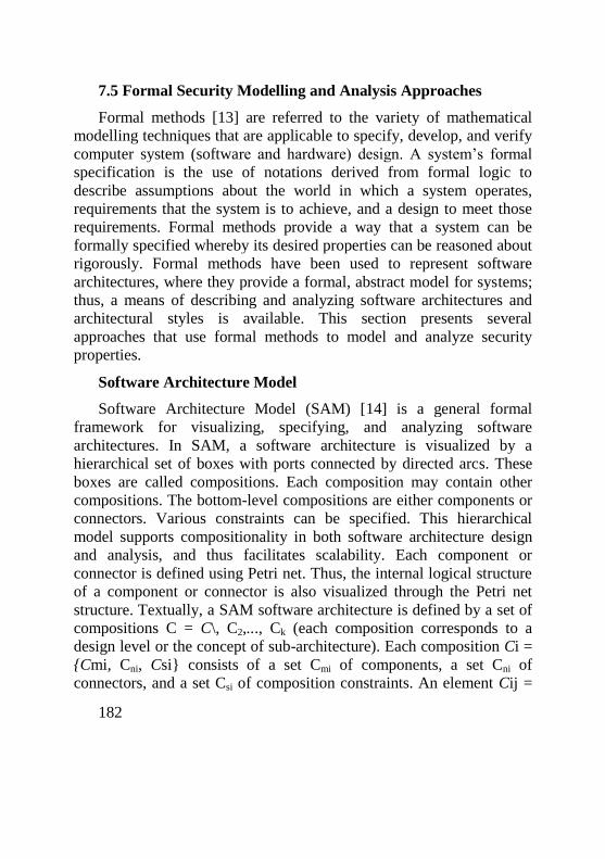
182

7.5 Formal Security Modelling and Analysis Approaches

Formal methods [13] are referred to the variety of mathematical

modelling techniques that are applicable to specify, develop, and verify

computer system (software and hardware) design. A system’s formal

specification is the use of notations derived from formal logic to

describe assumptions about the world in which a system operates,

requirements that the system is to achieve, and a design to meet those

requirements. Formal methods provide a way that a system can be

formally specified whereby its desired properties can be reasoned about

rigorously. Formal methods have been used to represent software

architectures, where they provide a formal, abstract model for systems;

thus, a means of describing and analyzing software architectures and

architectural styles is available. This section presents several

approaches that use formal methods to model and analyze security

properties.

Software Architecture Model

Software Architecture Model (SAM) [14] is a general formal

framework for visualizing, specifying, and analyzing software

architectures. In SAM, a software architecture is visualized by a

hierarchical set of boxes with ports connected by directed arcs. These

boxes are called compositions. Each composition may contain other

compositions. The bottom-level compositions are either components or

connectors. Various constraints can be specified. This hierarchical

model supports compositionality in both software architecture design

and analysis, and thus facilitates scalability. Each component or

connector is defined using Petri net. Thus, the internal logical structure

of a component or connector is also visualized through the Petri net

structure. Textually, a SAM software architecture is defined by a set of

compositions C = C\, C2,..., Ck (each composition corresponds to a

design level or the concept of sub-architecture). Each composition Ci =

{Cmi, Cni, Csi} consists of a set Cmi of components, a set Cni of

connectors, and a set Csi of composition constraints. An element Cij =

183

(Sij, Bij), (either a component or a connector) in a composition Ci has a

property specification Sij (a temporal logic formula) and a behavior

model Bij (Petri net). Each composition constraint in Csi is also defined

by a temporal logic formula. The interface of a behavior model Bij

consists of a set of places (called ports) that is the intersection among

relevant components and connectors. Each property specification Sij

only uses the ports as its atomic propositions/predicates that are true in

a given marking if they contain appropriate tokens. A composition

constraint is defined as a property specification, however it often

contains ports belonging to multiple components and/or connectors. A

component Cij can be refined into a lower-level composition Ci, which

is defined by h(Cij) = C;(h is a hierarchical mapping relating

compositions). The behavior of an overall software architecture is

derived by composing the bottom-level behavior models of components

and connectors. SAM provides both the modelling power and flexibility

through the choice of different Petri net models. In SAM, software

architecture properties are specified using a temporal logic. Depending

on the given Petri net models, different temporal logics are used.

In [15], SAM is applied to support the formal design of software

architecture for secure distributed systems. The security problem

addressed is general information confidentiality (refer to Figure 7.1).

The Petri net model used is the Predicate Transition Nets. The linear-

time temporal logic is selected to formally specify security policies, the

Chinese Wall policy, where Basic objects are individual items of

information (e.g. files), each concerning a single corporation; Company

datasets define groups of objects that refer to the same corporation;

Conflict of interest classes (COI) define company datasets that refer to

competing corporations. Subsequently, the definition of the sensitive

dataset and secure distributed control architecture are provided. Finally,

a new concept called the dependence relation for the Petri net model is

defined, which gives source and sink of every work flow in the model

and the dominating elements. Given an architecture model of a

distributed system, a set of rules have been given to reconstruct the

software architecture and enforce the security policy in the workflow

184

level for a software architecture by examining the flow of sensitive

datasets between tasks.

The strength of the approach is that it integrates two formalisms,

Petri nets and temporal logic, to specify software architectures. The

properties of the software architecture (e.g., information flow,

deadlock, etc.) specified in Petri nets can be proved using temporal

logic. Consequently, model checking techniques can be employed to

realize the automated verification of software architecture properties. In

addition, the approach provides a hierarchical architecture specification

model, which enables iterative model checking in a bottom-up fashion.

However, one issue of the approach is because of the limitation of

model checking, the approach is generally not applicable to infinite

state systems.

Multi Security Level Architecture

A modelling method for the Multilevel Security (MLS) architecture

of the Defense Advanced Research Projects Agency’s (DARPA’s)

Polymorphous Computing Architecture (PCA) program is proposed in

[16]. PCA is a multi-processor architecture that allows a processor to

morph during operations to provide the best type of processor for the

job at hand. The goal of MLS-PCA is to create a high assurance

security infrastructure for multiprocessor distributed applications,

which means that the trusted aspects of the system needs to be verified,

at a high level, under a certification program, such as the DoD's Trusted

Computer Security Evaluation Criteria or its replacement, the Common

Criteria (CC). In the proposed architecture, each single level Avionics

Application Process (AAP) is front-ended by an Encryption Processing

Element (EPE). All communication by an AAP must go through an

EPE. All communication between EPEs is encrypted and authenticated.

Keys are distributed to the EPEs by the Network Security Element

(NSE) based on a security policy set up by mission control. The NSE

enforces both Mandatory Access Control (MAC) and Discretionary

Access Control (DAC). There is a unique key for each element of the

security policy. For example, there is a key for each security level and

185

compartment in the MAC security lattice, as well as for each pair in the

DAC matrix. The NSE generates a session key between two AAPs by

XORing the relevant policy keys with a onetime random key. The

session key is then distributed to each of the AAP's EPE, where this

session key must be distributed encrypted. All connections between two

AAPs are simple. This allows a low level process to send information

up to a high level process, but not vice versa. Another type of

connection, called a coalition, that consists of AAPs at a common

security level and using a common key is also allowed. In addition, the

EPEs are also transparent to the AAPs, preventing the EPEs themselves

from being used as a covert channel. High levels of evaluation require

formal models and analysis. The selected formal method is Alloy [17].

The language is based on set theory and the first-order logic, similar to

Z, with the standard set operators and quantifiers. A state is defined by

sets and relationships among them. An operation will transform a state

to a new state, i.e., the sets are modified. Alloy also allows the

specification of invariants.

The security problem addressed in the approach is authentication

(refer to Figure 7.1). With the use of formal method Alloy and its

analysis tool in the approach, one can check the correctness of software

architecture specification, using an inductive argument to claim that if

an initial state is legal and all operations produce legal states, the

system cannot be in an illegal state and the specification is correct. The

approach also can be used to determine if a software architecture

specification is overconstrained or under-constrained. The approach

forces designers to look at the details of the architecture at an early

stage of development, thus problems are detected and verification

provides evidence that the requirements are maintained. One issue of

the approach is: as in the analysis of an Alloy specification, a solution

is obtained in a specific scope, therefore, the analysis of the approach is

correct, but not complete.

186

Security Check

Security check is a technique proposed in [18] to entail taking small

units of a system, putting them in a “security harness” that exercises

relevant executions appropriately within the unit, and then model

checking these tractable units. The technique is inspired by unit

verification. The basic semantic framework used in the modelling is

discrete time labeled transition systems. A discrete-time transition

labeled transition system (DTLTS) is a tuple < S,A sj > where: S is a

set of states; A is a visible action set; ^ is the transition relation; and sj

is the start state. The distinguished elements t and i correspond to the

internal action and clock-tick (or idling) action. A DTLTS encodes the

operational behavior of a real time system. States may be seen as

“configurations” the system may enter, while actions represent

interactions with the system’s environment that can cause state

changes. The transition relation records which state changes may occur:

if < s, a, s' > is a transition relation, then the transition from state s to s'

may take place whenever action a is enabled. t is always enabled; other

actions may require “permission” from the environment in order to be

enabled. Also, transitions except those labeled by i are assumed to be

instantaneous. While unrealistic at a certain level, this assumption is

mathematically convenient, and realistic systems, in which all

transitions “take time”, can be easily modelled. If a DTLTS satisfying

the maximal progress property is in a state in which internal

computation is possible, then no idling (clock ticks) can occur. DTLTSs

model the passage of time and interactions with a system’s

environment. Finally, DTLTSs may be minimized by merging

semantically equivalent but distinct states. The properties prove in

security check are safety properties, including quasiliveness or bounded

response which is a reasonable weakening of classical liveness. Both

these classes of properties are inherent in any security property

specification. While safety deals with properties of the form “nothing

bad will happen” (i.e., the private key can never be revealed), liveness

deals with assured- response or in a temporal setting bounded-response

187

(i.e., the system will always respond in “t” time units even when under

a DOS attack). Security check works by taking the property to be

proved on the system and suitably crafting a “test process” based on

that property (safety or liveness). The “unit”, or modules inside the

system to which the property is applicable, is isolated, all the behavior

of the process not relevant to the property in question is “sealed” off

and this transformed “unit” is first minimized and then run in parallel

with the test process. Then it is checked if the test process terminates by

emitting a pre-designated “good” or a “bad” transition. Depending on

the transition the test process emitted it can be decided if a property is

satisfied by the system or not.

The security problem addressed in the approach is to improve the

intrusion detection capabilities for distributed system. The security

check approach offers a means of coping with state explosion of a

system. The approach also enables to detect system vulnerabilities even

when the attack behavior is not known. And for known attack patterns

the approach can provide models of suspicious behavior which can then

be used for intrusion detection at a later stage. One issue of the

approach is since modelling checking techniques have been used; the

approach is more suitable to finite state systems.

CVS-Server Security Architecture

An outline of a formal security analysis of a CVS-Server

architecture is presented in [19]. The analysis is based on an abstract

architecture (enforcing a role-based access control on the repository),

which is refined to an implementation architecture based on the usual

discretionary access control provided by the POSIX environment). The

Concurrent Versions System (CVS) is a widely used tool for version

management in many industrial software development projects, and

plays a key role in open source projects usually performed by highly

distributed teams. CVS provides a central database (the repository) and

means to synchronize local modifications of partial copies (the working

copies) with the global repository. CVS can be accessed via a network;

this requires a security architecture establishing authentication, access

188

control and non-repudiation. The proposed architecture aims to provide

an improved CVS server, which overcomes the shortcomings of the

default CVS server. The first aim of the work is to provide a particular

configuration of a CVS server that enforces a role-based access control

security policy. The second aim is to develop an “open CVS-Server

architecture”, where the repository is part of the usual shared file

system of a local network and the server is a regular process on a

machine in this network. While such an architecture has a number of

advantages, the correctness and trustworthiness of the security

mechanisms become a major concern, which leads to use formal

methods to analyzing the access control problem of complex system

technology and its configuration. The formal method Z has been chosen

as the specification formalism. The modelling and theorem proving

environment Isabelle/HOL-Z 2.0 is used, which is an integrated

documentation, type- checking, and theorem proving environment for Z

specifications.

The security problem addressed in the approach is role- based

access control (refer to Figure 7.1), which is modelled and analyzed in

the context of a CVS system. Therefore, the RBAC addressed in the

approach is not generic to other applications.

7.6 Integrated Semi-formal and Formal Modelling and Analysis

Approaches

This section presents the approaches that use a combination of

semi-formal and formal methods to model and analyze security non-

functional properties.

UML/Theorem Prover Approach

An extensible verification framework for verifying UML models

for security requirements is presented in [20]. In particular, it includes

various plug-ins performing different security analysis on models of the

security extension UMLsec. Then an automated theorem prover binding

is used to verify security properties of UMLsec models that make use

of cryptography (such as cryptographic protocols). The UMLsec is an

189

extension to UML that allows the expression of security relevant

information within the diagrams in a system specification. UMLsec is

defined in the form of a UML profile using the standard UML

extension mechanism. The analysis routine in the verification

framework supports the construction of automated requirements

analysis tools for UML diagrams. The framework is connected to

industrial CASE tools using data integration with XMI and allows

convenient access to this data and to the human user. Advanced users of

the UMLsec approach should be able to use this framework to

implement verification routines for the constraints of self-defined

stereotypes, in a way that allows them to concentrate on the verification

logic (rather than on user interface issues). The usage of the framework

proceeds as follows: the developer creates a model and stores it in the

UML 1.4/XMI 1.2 file format; the file is imported by the UML

verification framework into the internal Metadata Repository (MDR).

MDR is an XMI-specific data-binding library that directly provides a

representation of an XMI file on the abstraction level of a UML model

through Java interfaces (JMI). This allows the developer to operate

directly with UML concepts, such as classes, statecharts, and

stereotypes. Each plug-in accesses the model through the JMI interfaces

generated by the MDR library. The plug-ins may receive additional

textual input and they may return both a UML model and textual

output. The plug-ins include static and dynamic checkers. The static

checker parses the model, verifies its static features, and delivers the

results to the error analyzer. The dynamic checker translates the

relevant fragments of the UML model into the automated theorem

prover input language. The automated theorem prover is spawned by

the UML framework as an external process; its results are delivered

back to the error analyzer. The error analyzer uses the information

received from the static checker and dynamic checker to produce a text

report for the developer describing the problems found, and a modified

UML model, where the errors found are visualized. Besides the

automated theorem prover binding presented in this chapter there are

190

other analysis plugins including a model-checker binding and plug-ins

for simulation and test-sequence generation.

The security problem addressed in the approach is authentication

(refer to Figure 7.1). The approach has been applied to a security-

critical biometric system, where the control access to protected

resources, such as a user’s biometric reference data, needs to be

ensured. Therefore, a cryptographic protocol is needed to protect the

communication between the user biometric data reader and the host

system. The protocol uses message counter in the transmission

messages, thus to detect attacks. With the application of the approach, a

flaw in the protocol, which allows attackers to misuse those message

counters, has been detected. However, security properties that can be

analyzed in the approach are limited to those which can be represented

in first-order logic.

UML/Promela Approach

The UML/Promela approach [21] is proposed to investigate an

appropriate template for security patterns that is tailored to meet the

needs of secure systems development. In order to maximize

comprehensibility, the well-known notation UML is used to represent

structural and behavioral information. Furthermore, the verification of

security properties is enabled by adding formal constraints to the

patterns. The enhanced security pattern template presented herein

contains additional information, including behavior, constraints, and

related security principles, that addresses difficulties inherent to the

development of security-critical systems. The security needs of a

system depend highly on the environment in which the system is

deployed. By introducing and connecting general security properties

with a pattern’s substance, the developer can gain security insight by

reading and applying the pattern. Furthermore, behavioral information

and security-related constraints are included in the security pattern

template. The developer can use this information to check if a specific

design and implementation of the pattern is consistent with the essential

security properties. The augmented security pattern template includes

191

fields’ applicability, behavior, constraints, consequences, related

security pattern, supported principles, and thus enhances the

communication of security-specific knowledge that is related to a

concrete application. Finally, a UML formalization framework that is

developed to support the generation of formally specified models

defined in terms of Promela [22], the language for the Spin model

checker, thus to analyze the security pattern related requirements.

The security problem addressed in the approach is authorization

(refer to Figure 7.1). The approach has been applied to an example

system, where security properties, such as access violations from

external requests to the system’s internal entities, can be verified. These

properties are instantiated in terms of linear time temporal logic to

enable the analysis with Spin model checker. However, the approach

currently focuses on the security property analysis against

requirements. It needs to be extended in order to support the

architecture level design and analysis of security properties.

7.7 Aspect-Oriented Security Modelling and Analysis

Approaches

The principle of separation of concerns has long been a core

principle in software engineering. It helps software engineers with

managing the complexity of software system development. This

principle refers to the ability to identify, encapsulate, and manipulate

those parts of software that are relevant to a particular concern

(concept, goal, purpose, non-functional properties, etc.). However,

many concerns of a system tend to crosscut many design elements at

the design level; their implementation tends to crosscut many code

units. Aspect-Oriented Software Development (AOSD) [23]

technologies have been proposed to enable the modularization of such

crosscutting concerns. In AOSD, a system’s tangling concerns or

pervasive properties are encapsulated in model element called an

aspect. Subsequently, a weaving process is employed to compose core

functionality model elements with these aspects, thereby generating an

architecture design. This section presents aspect-oriented approaches

192

which have been proposed to model and analyze security nonfunctional

properties.

Aspect-Oriented Secure Application

An experience report based on developing security solutions for

application software is presented in [24]. The programming language

AspectJ [25] is used for this purpose. The engineering of application

level security requirements are considered in this report, where the

security concern covers many aspects, including authentication,

auditing, authorization, confidentiality, integrity and non-repudiation.

Security is a pervasive requirement for an application. Modularizing

security concerns is a difficult task, and where and when to call a given

security mechanism in an application has not been addressed

adequately either. Furthermore, the crosscutting nature of security not

only relates to the diversity of specific places where security

mechanisms are to be called: some security mechanisms also require

information that is not localized in the application. An example used in

the report describes a Personal Information Management (PIM) system.

A PIM system supports the human memory by keeping track of

personal information, including a person’s agenda, contact information

of friends and business contacts, the tasks he has to fulfill, etc. A palm

pilot is a typical example of a PIM system. In this system, the security

requirement is the enforcement of access control. The design of this

application is captured in a UML class diagram, where a class called

PIMSystem is the center of the model. Through this class, the system

can represent and manage three different types of information:

appointments, contacts and tasks. Two security access rules are: for

appointments and tasks, the owner can invoke all their operations; other

persons are only allowed to view them; for contacts, only owners can

perform their operations. Finally, the report focuses on implementing

these rules as aspects in AspectJ.

The security problem addressed in the approach is authorization

(refer to Figure 7.1). The approach provides a way to implement

authorization properties as crosscutting concerns in the aspect-oriented

193

programming language AspectJ. However, it did not address the

problem of aspect-oriented design of security properties.

Formal Design Analysis Framework

Formal Design Analysis Framework (FDAF) [26, 27, 28], is an

aspect-oriented approach proposed to support the design and automated

analysis of non-functional properties for software architectures. In the

FDAF, non-functional properties are represented as aspects. At the

architecture design level, aspect represents either a property that

permeates all or part of a system, or a desired functionality that may

affect the behavior of more than one architecture design elements, such

as security aspects. Security aspects, including data origin

authentication, role-based access control, and log for audit, have been

defined in the FDAF. The definition of these security aspects uses

UML diagrams. The definition for a security aspect includes its static

view and dynamic view. The static view of a security aspect is defined

using UML class diagram, presenting the attributes and operations need

to be used in order to include the desired functionality in a system. It

may also include OCL invariants, pre-conditions, and post-conditions

regarding the weaving constraints of the security aspect. The dynamic

view of a security aspect is defined in UML sequence diagram,

describing the dynamic behavior of the security aspect, including the

information about when and where to use the operations defined in the

security aspect’s static view. The FDAF proposes a UML extension to

support the modelling of security aspects in UML. This extension

assists architects in weaving an aspect into a design and updating an as-

pect in a design. The syntax and semantics for this UML extension have

been defined. The FDAF uses a set of existing formal analysis tools to

automatically analyze a UML architecture design that has been

extended with security aspects. Architecture designs are documented

using extended UML class diagram and swim lane activity diagram in

the FDAF. The automated analysis of an extended UML architecture

design in existing formal analysis tools is achieved by formalizing part

of UML into a set of formal languages that have tool support. The

194

translation into a formal language with existing tool support leverages a

large body of work in the research community. The formalization

approach used is the translational semantic approach [29]. In

translational semantics, models specified in one language are given

semantics by defining a mapping to a simpler language, or a language,

which is better understood. Algorithms for mapping UML class and

swim lane activity diagrams to a set of formal languages have been

defined, verified with proofs, and implemented in the FDAF tool

support, thus automated translation from UML to this set of formal

languages are realized. Formal languages that UML can be formalized

in the FDAF for the analysis of security properties include Promela [22]

and Alloy [17], where Promela’s analysis tool is used to analyze data

origin authentication and log for audit security aspect design and

Alloy’s analysis tool is used to analyze role-based access control

security aspect UML design.

The example system selected in the FDAF is the Domain Name

System (DNS) [30], which is a real-time, distributed system. The

security problem addressed includes data origin authentication, role-

based access control, and log for audit (refer to Figure 7.1). There three

security aspects have been modelled in the DNS, where data origin

authentication is used to ensure the source of data, role-based access

control is used to ensure the access control of the DNS database, and

log for audit is used to log DNS messages. The strength of the approach

is it integrates the well-known semi-formal notation UML and a set of

existing formal notations into an aspect-oriented architectural

framework to support the design and analysis of non-functional

properties, such as security and performance. A limitation of the

approach is that the analysis of a UML based architecture design uses

existing formal tools, the limitations of these tools affect the analysis

results provided in terms of accuracy, useful analysis data extraction,

and interpretation of the results.

195

7.8 Discussion

A summary of the approaches in the survey is presented in Table

7.1. The approaches in this survey support modelling of one or more

security properties at the architecture design level; many also support

their automated analysis. The comparison criteria defined for this

survey are: identifying the specific security property addressed (e.g.,

role-based access control, authentication, etc.), modelling notation(s)

used, whether or not automated security property analysis is supported,

and the kind of example system the approach has been applied to. Each

of these criteria is useful, as the results can be used to guide the

selection of an appropriate approach and identify possible areas for

future research. For example, if one needs to model (but perhaps not

analyze) role-based access control for a distributed system, then UML

can be selected as the modelling notation. However, if there is a need

for a more rigorous, automated analysis of the security property, then a

formal method would be more suitable, such as Z or Alloy. If one needs

to model confidentiality for information system, then Petri nets and

temporal logic are candidate notations, as these have been already been

successfully used to model this property. This is not to say that other

notations could not be used to model confidentiality. Actually, it opens

a wide variety of possible future research topics that investigate the use

of different notations, tailored notations, and perhaps identifying a set

of notations that are suitable for modelling a comprehensive collection

of security properties. It is also important to note that the validation of

the approaches presented in the literature has typically been made using

one example system. Additional validation of the approaches used to

model and analyze security properties for the architecture design is

necessary.

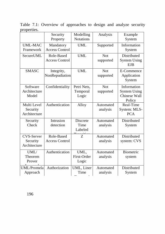
196

Table 7.1: Overview of approaches to design and analyze security

properties. Security

Property

Modelling

Notations

Analysis Example

System

UML-MAC

Framework

Mandatory

Access Control

UML Supported Information

System

SecureUML Role-Based

Access Control

UML Not

supported

Distributed

System Using

EJB

SMASC Integrity,

NonRepudiation

UML Not

supported

E-Commence

Application

System

Software

Architecture

Model

Confidentiality Petri Nets,

Temporal

Logic

Not

supported

Information

System Using

Chinese Wall

Policy

Multi Level

Security

Architecture

Authentication Alloy Automated

analysis

Real-Time

System: MLS-

PCA

Security

Check

Intrusion

detection

Discrete

Time

Labeled

Transition

System

Automated

analysis

Distributed

System

CVS-Server

Security

Architecture

Role-Based

Access Control

Z Automated

analysis

Distributed

system: CVS

UML/

Theorem

Prover

Approach

Authentication UML,

First-Order

Logic

Automated

analysis

Biometric

system

UML/Promela

Approach

Authorization UML, Liner

Time

Temporal

Logic

Automated

analysis

Distributed

System

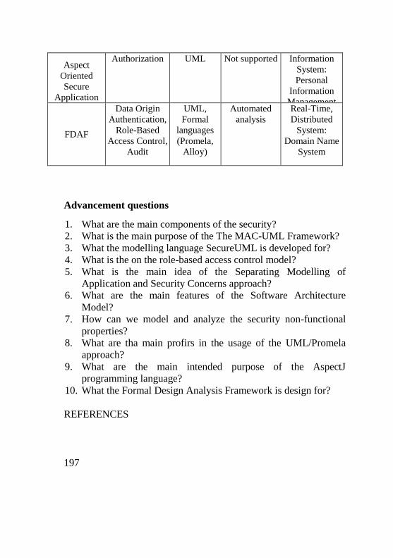
197

Aspect

Oriented

Secure

Application

Authorization UML Not supported Information

System:

Personal

Information

Management

System

FDAF

Data Origin

Authentication,

Role-Based

Access Control,

Audit

UML,

Formal

languages

(Promela,

Alloy)

Automated

analysis

Real-Time,

Distributed

System:

Domain Name

System

Advancement questions

1. What are the main components of the security?

2. What is the main purpose of the The MAC-UML Framework?

3. What the modelling language SecureUML is developed for?

4. What is the on the role-based access control model?

5. What is the main idea of the Separating Modelling of

Application and Security Concerns approach?

6. What are the main features of the Software Architecture

Model?

7. How can we model and analyze the security non-functional

properties?

8. What are tha main profirs in the usage of the UML/Promela

approach?

9. What are the main intended purpose of the AspectJ

programming language?

10. What the Formal Design Analysis Framework is design for?

REFERENCES

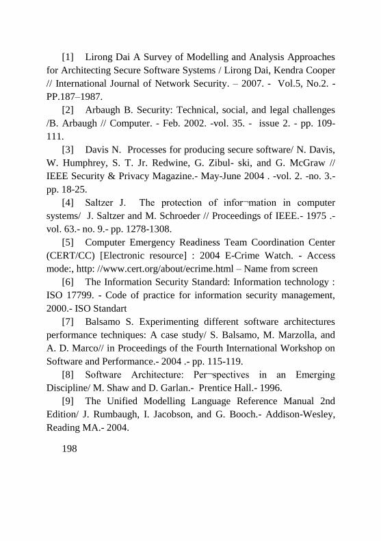
198

[1] Lirong Dai A Survey of Modelling and Analysis Approaches

for Architecting Secure Software Systems / Lirong Dai, Kendra Cooper

// International Journal of Network Security. – 2007. - Vol.5, No.2. -

PP.187–1987.

[2] Arbaugh B. Security: Technical, social, and legal challenges

/B. Arbaugh // Computer. - Feb. 2002. -vol. 35. - issue 2. - pp. 109-

111.

[3] Davis N. Processes for producing secure software/ N. Davis,

W. Humphrey, S. T. Jr. Redwine, G. Zibul- ski, and G. McGraw //

IEEE Security & Privacy Magazine.- May-June 2004 . -vol. 2. -no. 3.-

pp. 18-25.

[4] Saltzer J. The protection of infor¬mation in computer

systems/ J. Saltzer and M. Schroeder // Proceedings of IEEE.- 1975 .-

vol. 63.- no. 9.- pp. 1278-1308.

[5] Computer Emergency Readiness Team Coordination Center

(CERT/CC) [Electronic resource] : 2004 E-Crime Watch. - Access

mode:, http: //www.cert.org/about/ecrime.html – Name from screen

[6] The Information Security Standard: Information technology :

ISO 17799. - Code of practice for information security management,

2000.- ISO Standart

[7] Balsamo S. Experimenting different software architectures

performance techniques: A case study/ S. Balsamo, M. Marzolla, and

A. D. Marco// in Proceedings of the Fourth International Workshop on

Software and Performance.- 2004 .- pp. 115-119.

[8] Software Architecture: Per¬spectives in an Emerging

Discipline/ M. Shaw and D. Garlan.- Prentice Hall.- 1996.

[9] The Unified Modelling Language Reference Manual 2nd

Edition/ J. Rumbaugh, I. Jacobson, and G. Booch.- Addison-Wesley,

Reading MA.- 2004.

199

[10] Doan T. MAC and UML for secure software design / T.

Doan, S. Demurjian, T. C. Ting, and A. Ket- terl// in Proceedings of the

2004 ACM Workshop on Formal Methods in Security Engineering.-

2004. - pp. 75-85.

[11] Lodderstedt T. Se- cureUML: A UML-based modelling

language for model-driven security / T. Lodderstedt, D. Basin, and J.

Doser // in Proceedings of the 5th International Conference on The

Unified Modelling Language. - 2002 . - pp. 426-441.

[12] Gomaa H. Modelling complex systems by separating

application and security concerns. / H. Gomaa and M. Eonsuk Shin //

in Proceedings of the Ninth IEEE International Conference on

Engineering Complex Computer Systems. -2004. - pp. 19-28.

[13] Bowen J. P. An invitation to formal methods / J. P. Bowen, R.

W. Butler, D. L. Dill, R. L. Glass, D. Gries, and A. Hall.// Computers. -

1996. - vol. 29, issue 4. - pp. 16-29,.

[14] He X. Formally analyzing software architectural

specifications using SAM / X. He, H. Yu, T. Shi, J. Ding, and Y. Deng

// Journal of Systems and Software/- 2004. - vol. 71, no. 1-2. - pp. 11-

29.

[15] Yu H. Formal software architecture design of secure

distributed systems / H. Yu, X. He, S. Gao, and Y. Deng // in

Proceedings of the Fifteenth International Conference on Software

Engineering and Knowledge Engineering (SEKE'03). - 2003. - vol. 1. -

pp. 450-457.

[16] Hashii B. Lessons learned using alloy to formally specify

MLS-PCA trusted security architecture / B. Hashii // in Proceedings of

the 2004 ACM Workshop on Formal Methods in Security

Engineering.- 2004. - vol. 1. - pp. 86-95.

200

[17] Software Design Group, the Alloy Analyzer [Electronic

resource]: 2002 – 2005. - Access mode: http://alloy.mit.edu.

[18] Ray A. Security check: a formal yet practical framework for

secure software architecture / A. Ray // in Proceedings of the 2003

Workshop on New Security Paradigms.- 2003. - vol. 1. - pp. 59-65.

[19] Brucker A. A case study of a formalized security architecture

/ A. Brucker, and B. Wolff // Electronics Notes in Theoretical

Computer Science. - 2003. - vol. 80. - pp. 1-18.

[20] Jurjens J. Sound methods and effective tools for model-based

security engineering with UML /J. Jurjens // in Proceedings of the 27th

International Conference on Software Engineering.- 2005. - vol. 1. -

322-331.

[21] Using Security Patterns to Model and Analyze Security

Requirements, Technical Report MSU-CSE- 03-18 / B. Cheng, S.

Honrad, L. Campbell, and R. Wasser- mann. - Department of Computer

Science, Michigan State University, 2003.

[22] The Spin Model Checker: Primer and Reference Manual / G.

J. Holzmann. - Addison-Wesley, 2003.

[23] Aspect- Oriented Software Development / R. Filman, T.

Elrad, S. Clarke, and M. Aksit. - Addison Wesley Professional, 2005.

[24] 30 Win B. Developing secure applications through aspect-

oriented programming / B. Win, W. Joosen, and f. Piessens // Aspect-

Oriented Software Development (ISBN: 0321219767). - 2005. - pp.

633-651.

[25] AspectJ in Action: Practical Aspect- Oriented Programming /

R. Laddad. - Manning Publications, 2003.

[26] Cooper K. Performance modelling and analysis of software

architectures: an aspect-oriented UML based approach / K. Cooper, L.

Dai, and Y. Deng // Journal of Science of Computer Programming,

201

System and Software Architectures. - July 2005. - vol. 57, no. 1. - pp.

89-108.

[27] Formal Design Analysis Framework: An Aspect-Oriented

Architectural Framework / L. Dai. - The University of Texas at Dallas,

Ph.D. Dissertation, 2005.

[28] Dai L. Modelling reusable security aspects for software

architectures: a pattern driven approach / L. Dai, K. Cooper, and E.

Wong // in Proceedings of the 17th International Conference on

Software Engineering and Knowledge Engineering. - July 2005. - pp.

163-168.

[29] Hofstede A. H. M. How to formalize It? Formalization

principles for information system development methods / A. H. M.

Hofstede, and H. A. Proper // Information and Software Technology. -

1998. - vol. 40, no. 10. - pp. 519-540,.

[30] Domain Names - Concepts and Facilities/ P. V. Mockapetris.

- IETF STD0013. - November, 1987

202

CHAPTER 8. FORMAL METHODS FOR ASSURING

SECURITY OF PROTOCOLS

Content of the CHAPTER 8

8.1 Security primer ........................................................................ 203

8.2 Needham–schroeder protocol .................................................. 206

8.3 Belief logics ............................................................................. 208

8.4 Process algebras ....................................................................... 211

8.5 Associating keys and principals .............................................. 220

8.6 Conclusions ............................................................................. 223

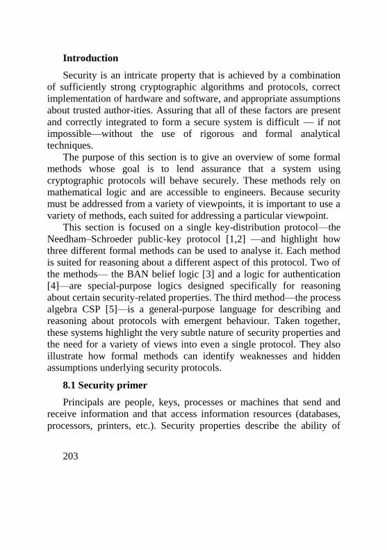
203

Introduction

Security is an intricate property that is achieved by a combination

of sufficiently strong cryptographic algorithms and protocols, correct

implementation of hardware and software, and appropriate assumptions

about trusted author-ities. Assuring that all of these factors are present

and correctly integrated to form a secure system is difficult — if not

impossible—without the use of rigorous and formal analytical

techniques.

The purpose of this section is to give an overview of some formal

methods whose goal is to lend assurance that a system using

cryptographic protocols will behave securely. These methods rely on

mathematical logic and are accessible to engineers. Because security

must be addressed from a variety of viewpoints, it is important to use a

variety of methods, each suited for addressing a particular viewpoint.

This section is focused on a single key-distribution protocol—the

Needham–Schroeder public-key protocol [1,2] —and highlight how

three different formal methods can be used to analyse it. Each method

is suited for reasoning about a different aspect of this protocol. Two of

the methods— the BAN belief logic [3] and a logic for authentication

[4]—are special-purpose logics designed specifically for reasoning

about certain security-related properties. The third method—the process

algebra CSP [5]—is a general-purpose language for describing and

reasoning about protocols with emergent behaviour. Taken together,

these systems highlight the very subtle nature of security properties and

the need for a variety of views into even a single protocol. They also

illustrate how formal methods can identify weaknesses and hidden

assumptions underlying security protocols.

8.1 Security primer

Principals are people, keys, processes or machines that send and

receive information and that access information resources (databases,

processors, printers, etc.). Security properties describe the ability of

204

principals to access information or resources. Key security properties

include:

- privacy or confidentiality: knowing with accuracy which

principals can read data;

- integrity: detecting corruption of information;

- authentication: knowing the identity of a principal or the source

of information;

- access control: restricting the use of a resource to privileged

principals;

- non-repudiation: preventing principals from subse-quently

denying their actions;

- availability of service: guaranteeing authorized princi-pals

always have access to services.

The Handbook of Applied Cryptography [6] describes each of these

properties in more detail.

Public-key infrastructure

In public-key cryptography, encryption and decryption are provided

through pairs of related keys: each principal has both a public key

(which is made known to others) and a private key (which should be

known only to the principal). These keys act as mutual inverses:

anything encoded with one of these keys may be decoded with the

other. Thus public-key cryptography supports both privacy and digital

signatures.

If principal A wishes to send a secret message M to principal B, she

encrypts M with B’s public key: intuitively, only B has knowledge of

his private key and hence only B can decrypt the message. In contrast,

if A wishes to sign a message M, she encrypts it with her own private

key: intuitively, anyone with access to her public key can verify her

signature, but no one should be able to forge her signature without

knowledge of her private key.

A public-key infrastructure (PKI) supports the distribution,

management and use of public keys and certificates to provide

authentication, privacy and other security properties. PKIs are based on

205

certification authorities that vouch for the integrity of cryptographic

information and they form the basis of current Internet security.

Basic security foundations

A system’s overall security depends on several items, including:

- the cryptographic strength of the system (e.g., the computational

infeasibility of decrypting messages without the proper keys);

- the protocols built on top of the cryptographic algorithms (e.g.,

the secure sockets layer (SSL) protocol used by web browsers);

- the correct association of specific cryptographic keys with

specific principals.

Cryptographic strength is assessed over time by a combination of

complexity analysis and resistance to cryptanalysis [7]. The use of

formal methods to analyse cryptographic strength is not addressed here.

Assessing security protocols often involves an analysis of ways to

defeat a protocol by using bits of previously successful protocol runs

(known as replay attacks) or by some form of impersonation (e.g., ‘man

in the middle’ attacks). These analyses are particularly important,

because these protocols are run repeatedly over time and typically over

public networks: many security protocols depend critically on the

freshness of secrets.

Associating cryptographic keys with principals is typi-cally done

using certificates that are digitally signed by recognized certification

authorities, as in the X.509 public-key certificate standard [8].

Determining the public key of a principal is done using a chain of

certificates that enable one principal to move from one certificate

authority to another in a secure (i.e. digitally signed and checked) way

to fetch and check the certificate of another principal. The network of

certification authorities is referred to as a trust model or trust topology.

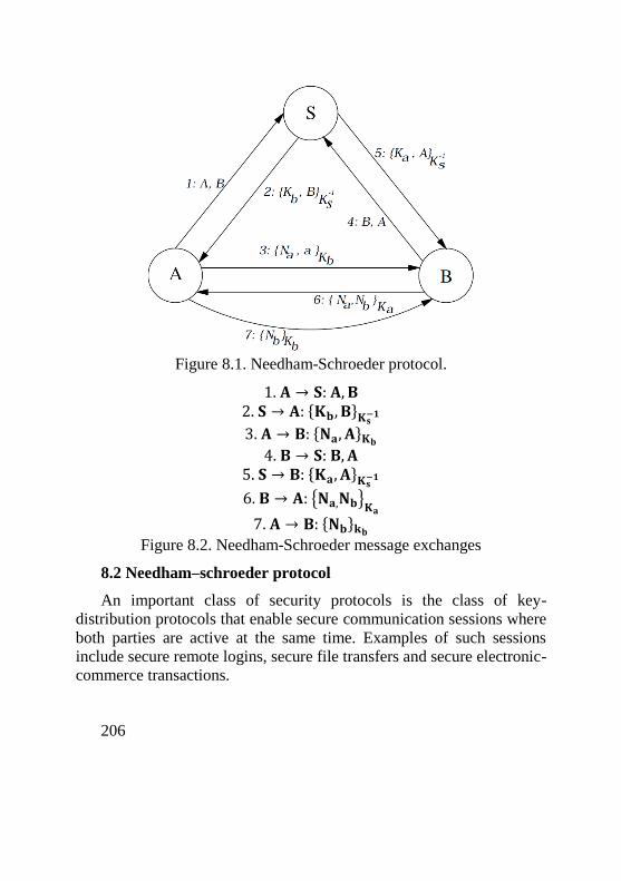
206

Figure 8.1. Needham-Schroeder protocol.

1. 𝐀 → 𝐒: 𝐀, 𝐁 2. 𝐒 → 𝐀: {𝐊𝐛, 𝐁}𝐊𝐬−𝟏

3. 𝐀 → 𝐁: {𝐍𝐚, 𝐀}𝐊𝐛

4. 𝐁 → 𝐒: 𝐁, 𝐀 5. 𝐒 → 𝐁: {𝐊𝐚, 𝐀}𝐊𝐬−𝟏

6. 𝐁 → 𝐀: {𝐍𝐚,𝐍𝐛}𝐊𝐚

7. 𝐀 → 𝐁: {𝐍𝐛}𝐤𝐛

Figure 8.2. Needham-Schroeder message exchanges

8.2 Needham–schroeder protocol

An important class of security protocols is the class of key-

distribution protocols that enable secure communication sessions where

both parties are active at the same time. Examples of such sessions

include secure remote logins, secure file transfers and secure electronic-

commerce transactions.

207

The Needham–Schroeder protocol [2] is designed to allow two

principals to mutually authenticate themselves through a series of

message exchanges, as a prelude for some secure session. A diagram of

the message exchanges appears in Figure 8.1, and Figure 8.2 details the

message exchanges in linear form.

In these descriptions, the principals are A, B and S, where S is a

certification authority (CA) recognized by principals A and B. Their

public keys are (respectively) Ka , Kb, and Ks; the private key of S

corresponding to the public key Ks is Ks−1

. Na and Nb are nonce

identifiers: a nonce is a fresh value created for the current run of a

protocol, which has not been seen in previous runs. Let us use common

notation for describing security protocols: A → B denotes principal A

sending a message to principal B; comma (‘,’) denotes conjunction or

concatenation (e.g., ‘X, Y ’ denotes a message containing both X and Y

); and {X}K denotes the message X encrypted using key K.

Principal A—wishing to communicate with principal B— must get

B’s public key from S and then convey a nonce Na to B (messages 1–3).

B then needs to get A’s public key from S and convey a nonce Nb to A

in such a way that convinces A that she is interacting with B (messages

4–6). Finally, A must convince B that he is interacting with A and that A

has received the nonce Nb (message 7).

Messages 1 and 2—as well as messages 4 and 5— correspond to

certificate requests from A and B to an authority S for the other’s public

key. As messages 1 and 4 are transmitted in the clear, they have no

cryptographic significance. In message 3, the nonce Na is conveyed to

B. Nevertheless, B cannot know for sure who sent Na : he must assume

that the identifier A is correct. In message 6, B sends to A both nonce Na

and Nb to identify himself as B to A, as well as to convey the nonce Nb

to A. The basic notion operating here is that A and B can identify shared

secrets (the nonces Na and Nb) to each other to convince each of the

other’s identity.

This protocol has several weaknesses, which are ad-dressed in the

subsequent sections. The principals in the protocol implicitly assume

that messages 2 and 5 are fresh and are not replays of messages

208

containing compromised keys; this situation is analysed on belief

logics. The protocol is also vulnerable to a ‘man in the middle’ attack.

8.3 Belief logics

One approach to reasoning about key-exchange protocols is to

analyse what principals believe about important components and

properties of protocols. These components include secret and public

keys, encrypted messages, messages combined with secrets, and nonces

(objects created for a specific run of a protocol). Important properties

include freshness (the property of never having been used in a prior run

of a protocol), jurisdiction or authority over keys, and binding of secret

and public keys to principals.

The Burroughs, Abadi and Needham (BAN) logic [3] is

representative of several belief logics [9, 10] that support reasoning

about these properties. It focuses on proving goals such as ‘A believes

Kb is B’s public key’. One of the central concerns that BAN logic

addresses is the possibility of replay attacks, where messages sent

during previously successful protocol runs are re-used or replayed to

trick principals into using compromised keys or to dupe principals into

thinking an intruder is a legitimate participant.

The notion of time in the BAN logic is very simple. Time is divided

into two categories: the present (i.e. the current run of the protocol) and

the past (i.e. any protocol run preceding the current run).

Syntax and semantics

Let us present only the subset of BAN logic’s syntax and semantics

necessary to describe part of the Needham– Schroeder protocol. A

complete description of BAN logic appears in [3]. The logic includes

the following types of statements.

- P |≡ X, read as ‘Principal P believes X’. P behaves as if X is true;

- P ◄ X, read as ‘P sees X’. A principal has sent P a message

containing X;

- P |∼ X, read as ‘P once said X’. P at some time (either in the

present or the past) believed X and sent it as part of a message;

209

- P |⇒ X, read as ‘P has jurisdiction over X’. Principal P has

authority over X and is trusted on this matter.

- # (X), read as ‘X is fresh’. X has not appeared in a past run of the

protocol. K|𝑲→P , read as ‘P has public key K’. The corresponding

private key is denoted by K−1 and assumed to be known only by

P;

While there are over 19 inference rules that define the semantics of

the BAN logic, the following three inference rules capture the essence

of the logic for public-key applications.

(1) Message-Meaning Rule for Public Keys. If P believes that Q’s

public key is K, and if P sees a message X encrypted with Q’s private

key K−1

, then P believes Q once said X:

𝑷|≡ |𝑲→ 𝐐 𝐏 < {𝐗}

𝐊−𝟏

𝑷 |≡(𝐐 |∼𝐗).

This rule uses the belief in the association of a public key with a

principal to establish the source of a message.

(2) Nonce-Verification Rule. If P believes that X is fresh (i.e. is

new to the current protocol run) and that Q once said X, then P believes

that Q believes X in the current run of the protocol: 𝑷|≡# (𝐗) 𝑷|≡(𝐐 |∼𝐗)

𝑷|≡(𝐐 |∼𝐗).

This rule uses the belief about the freshness of a message (usually

based on nonces), coupled with knowing the message source, to

establish that a principal uttered a message in the current protocol run.

(3) Jurisdiction Rule. If P believes that Q has authority over X

and that Q believes X, then P will believe in X:

𝑷|≡(𝐐⇒ 𝐗) 𝑷|(𝐐|≡𝐗 )

𝑷 |≡𝐗.

This rule applies to certification authorities. A principal will adopt

an authority’s belief if that principal recognizes the certification

authority. For example, if 𝑷| ≡ (𝐐 | ≡ 𝐊𝐛→ 𝐁) and 𝑷| ≡ (𝐐 ⇒

210

(𝐊𝐛→ 𝐁)) then 𝑷 | ≡

𝐊𝐛→ 𝑩.That is, P believes Kb is B’s public key when

P recognizes Q as a key certification authority.

Analysis of the protocol

When the Needham–Schroeder protocol is analysed using the BAN

logic, two possible weaknesses come to light. In steps 2 and 5 of the

protocol, certification authority S sends to A and B (respectively) the

messages {𝑲𝒃, 𝑩}𝑲𝒔−𝟏 and {𝑲𝒃, 𝑨}𝑲𝒔−𝟏; that is, A and B both receive the

public key of the principal with whom they wish to communicate.

After A receives {𝑲𝒃, 𝑩}𝑲𝒔−𝟏 in step 2, the desired result on A's

behalf is 𝑨 | ≡ (𝑲𝒃→ 𝑩): believes that 𝑲𝒃 is B's public key. From the

Jurisdiction Rule, this requires two other beliefs:

𝑨| ≡ (𝑺 ⇒ (𝑲𝒃→ 𝑩)) (1)

𝑨| ≡ (𝑺 | ≡ (𝑲𝒃→ 𝑩)) (2)

That is, A must believe that S has authority over 𝑲𝒃 and that S

believes 𝑲𝒃 is B's public key.

The first belief corresponds to A believing that S is a certification

authority having the proper authority to certify B's cryptographic

information. This is a reasonable assumption. Establishing the second

belief requires the application of both the Message-Meaning and

Nonce-Verification Rules.

It is reasonable to assume that A knows S's public key: (і. е. 𝑨| ≡ (𝑲𝒔→ 𝑺)) From the Message-Meaning Rule and the receipt of certificate

{𝑲𝒃, 𝑩}𝑲𝒔−𝟏 from S we can establish that 𝑨 | ≡ (𝑺 | ∼ (𝐊𝐛→ 𝐁)).

That is, A believes that S once said that 𝑲𝒃 was B's public key. We

can then use the Nonce-Verification Rule to establish that 𝑨| ≡ (𝐒| ≡ (𝐊𝐛→ 𝐁)), that 𝑨| ≡ #(

𝐊𝐛→ 𝐁). This proviso highlights a potential

weakness, as there is nothing in message 2 that corresponds to a nonce:

211

A must assume that anything with the public key from the authority S is

fresh. Consequently, the protocol is potentially vulnerable to a replay

attack based on reusing old keys.

A similar analysis holds true for A’s public key in step 5.

8.4 Process algebras

Process algebras such as CSP [5, 11] and CCS [12] provide a way

to describe system behaviour in terms of the events (i.e. abstract actions

deemed ‘observable’) that can occur. The collection of events that a

process can engage in is known as its alphabet, typically denoted by _.

The trace model of CSP formally describes a process’s behaviour in

terms of the set of traces—that is, sequences of events—that it can

perform. These trace sets provide a basis for comparing, equating and

refining processes. Two processes are trace-equivalent when they have

precisely the same sets of traces. A process Q refines P in the trace

model (written P Q) if every trace of Q is also a trace of P . Intuitively,

if P corresponds to a specification of permissible behaviour and Q

refines P , then Q is guaranteed to exhibit only permissible behaviours.

Using the trace model and the FDR2 model checker [13], Lowe

uncovered a previously unknown flaw in the Needham–Schroeder

protocol [14, 15]. An informal description of the approach in this

section, first introducing the relevant CSP notation is provided.

CSP syntax and semantics

Informally, CSP processes (ranged over by P ) can have the

following forms.

- STOP is the process that does nothing;

- e → P performs event e and then behaves like P;

- P1 ᴨ P2 non-deterministically chooses to behave like P1 or to

behave like P2.

- P1 [|X|] P2 is a parallel composition of P1 and P2, where the set

of events X constrains certain actions. Any event in the set X can

occur only if P1 and P2 both perform it simultaneously; in

212

contrast, events in ∑ - X occur only as independent actions of P1

or P2;

- P \X behaves like P, but the events in X are hidden (i.e.

considered unobservable);

- P [e1 ← e1_, . . . , en ← en_] behaves like P, except that each

event ei is relabelled to ei_. As a special case, in P [e ← e1, e ←

e2], the event e is replaced by a non-deterministic choice

between the events e1 and e2.

Formally, we introduce a family of relations 𝒂⇒ that describe

processes’ trace behaviour, writing 𝑷𝒂⇒ 𝑷′ to indicate that process P

can perform the trace a and become the process 𝑃′ This family of

relations can be defined as the smallest relations satisfying the axioms

and inference rules in Figure 8.3. The first two rules are primarily

bookkeeping rules: the first expresses that every process, by doing

nothing (_ denotes the empty trace), remains unchanged; the second

reflects that computations’ intermediate states can be abstracted away (·

denotes sequence concatenation). The remaining rules are syntax-

directed and formalize the informal explanations of the different

process terms given previously. In particular, there is no explicit rule

for STOP, because STOP never does anything.

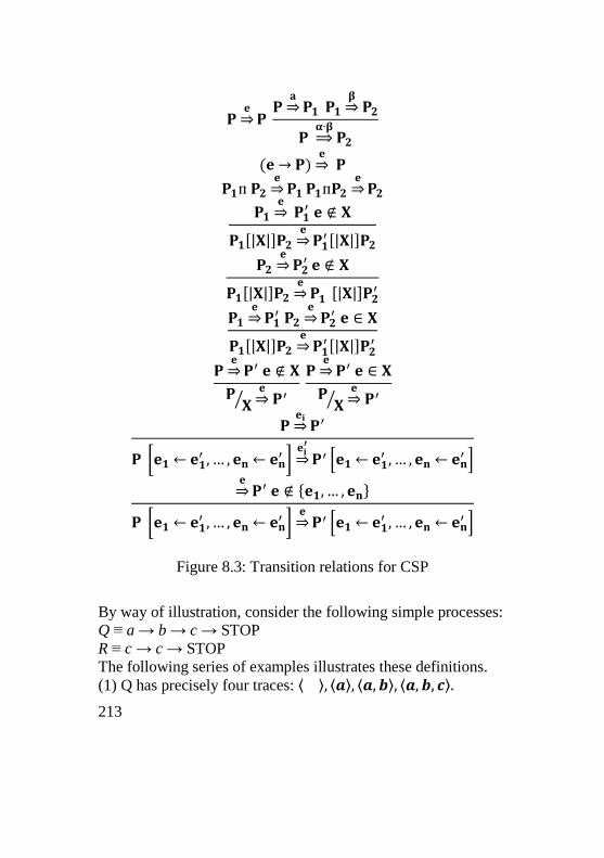
213

𝐏𝐞⇒𝐏

𝐏𝐚⇒𝐏𝟏 𝐏𝟏

𝛃⇒𝐏𝟐

𝐏 𝛂∙𝛃⇒ 𝐏𝟐

(𝐞 → 𝐏)𝐞⇒ 𝐏

𝐏𝟏ᴨ 𝐏𝟐𝐞⇒𝐏𝟏 𝐏𝟏ᴨ𝐏𝟐

𝐞⇒𝐏𝟐

𝐏𝟏𝐞⇒ 𝐏𝟏

′ 𝐞 ∉ 𝐗

𝐏𝟏[|𝐗|]𝐏𝟐𝐞⇒𝐏𝟏

′ [|𝐗|]𝐏𝟐

𝐏𝟐𝐞⇒𝐏𝟐

′ 𝐞 ∉ 𝐗

𝐏𝟏[|𝐗|]𝐏𝟐𝐞⇒𝐏𝟏 [|𝐗|]𝐏𝟐

′

𝐏𝟏𝐞⇒𝐏𝟏

′ 𝐏𝟐𝐞⇒𝐏𝟐

′ 𝐞 ∈ 𝐗

𝐏𝟏[|𝐗|]𝐏𝟐𝐞⇒𝐏𝟏

′ [|𝐗|]𝐏𝟐′

𝐏𝐞⇒𝐏′ 𝐞 ∉ 𝐗

𝐏𝐗⁄𝐞⇒𝐏′

𝐏𝐞⇒𝐏′ 𝐞 ∈ 𝐗

𝐏𝐗⁄𝐞⇒𝐏′

𝐏𝐞𝐢⇒𝐏′

𝐏 [𝐞𝟏 ← 𝐞𝟏′ , … , 𝐞𝐧 ← 𝐞𝐧

′ ]𝐞𝐢′

⇒𝐏′ [𝐞𝟏← 𝐞𝟏′ , … , 𝐞𝐧 ← 𝐞𝐧

′ ]

𝐞⇒𝐏′ 𝐞 ∉ {𝐞𝟏, … , 𝐞𝐧}

𝐏 [𝐞𝟏 ← 𝐞𝟏′ , … , 𝐞𝐧 ← 𝐞𝐧

′ ]𝐞⇒𝐏′ [𝐞𝟏← 𝐞𝟏

′ , … , 𝐞𝐧 ← 𝐞𝐧′ ]

Figure 8.3: Transition relations for CSP

By way of illustration, consider the following simple processes:

Q ≡ a → b → c → STOP

R ≡ c → c → STOP

The following series of examples illustrates these definitions.

(1) Q has precisely four traces: ⟨ ⟩, ⟨𝒂⟩, ⟨𝒂, 𝒃⟩, ⟨𝒂, 𝒃, 𝒄⟩.

214

(2) The traces of Q ᴨ R are simply those of Q and R:

⟨ ⟩, ⟨𝒂⟩, ⟨𝒂, 𝒃⟩, ⟨𝒂, 𝒃, 𝒄⟩, ⟨𝒄⟩, ⟨𝒄, 𝒄⟩. (3) The parallel composition Q [|{b, d}|] R has the following traces:

⟨ ⟩, ⟨𝒂⟩, ⟨𝒄⟩, ⟨𝒂, 𝒄⟩, ⟨𝒄, 𝒂⟩, ⟨𝒄, 𝒄⟩, ⟨𝒂, 𝒄, 𝒄⟩, ⟨𝒄, 𝒂, 𝒄⟩, ⟨𝒄, 𝒄, 𝒂⟩. Note that Q, denied cooperation from R, is unable

to perform its b event.

(4) In contrast, Q [|{c, d}|] R has these four traces:

⟨ ⟩, ⟨𝒂⟩, ⟨𝒂, 𝒃⟩, ⟨𝒂, 𝒃, 𝒄⟩. R must delay c events until Q is ready to

cooperate; furthermore, R can only perform one c event, because Q

provides only one opportunity to do so.

(5) The traces of (Q ᴨ R)\{b, d} are as follows:

⟨ ⟩, ⟨𝒂⟩, ⟨𝒂, 𝒄⟩, ⟨𝒄⟩, ⟨𝒄, 𝒄⟩. (6) Finally, (Q ᴨ R)[b ← a, c ← e, c ← d] has precisely these

traces: ⟨ ⟩, ⟨𝒂⟩, ⟨𝒂, 𝒂⟩, ⟨𝒂, 𝒂, 𝒅⟩, ⟨𝒂, 𝒂, 𝒆⟩, ⟨𝒅⟩, ⟨𝒆⟩, ⟨𝒅, 𝒅⟩, ⟨𝒅, 𝒆⟩, ⟨𝒆, 𝒅⟩, ⟨𝒆, 𝒆⟩. Note that every occurrence of b in a trace of Q ᴨ R is replaced by

a; every occurrence of c is replaced either by d or by e.

In practice, it is useful to have events with multiple fields: for

example, a description of a bank account might use events such as

deposit.50, deposit.100 and withdraw.100. Furthermore, a bank account

should be prepared to accept deposits of any amount: the notation

deposit?x represents a choice among all deposit events and the variable

x becomes bound to the actual value of the second field. Thus, for

example, the process in?w → out.w → STOP has among its traces ⟨𝒊𝒏. 𝟏𝟑, 𝒐𝒖𝒕. 𝟏𝟑 ⟩ and ⟨𝒊𝒏. 𝟒𝟓, 𝒐𝒖𝒕. 𝟒𝟓 ⟩.

Modelling the protocol’s messages

For simplicity of presentation, let us consider a simplified version

of the protocol in which A and B already know each other’s public

keys. Under these circumstances, A and B can forgo the

communications with the key server S, resulting in a protocol in which

only three messages need to be exchanged:

- A → B : {Na , A}Kb;

- B → A : {Na , Nb}Ka;

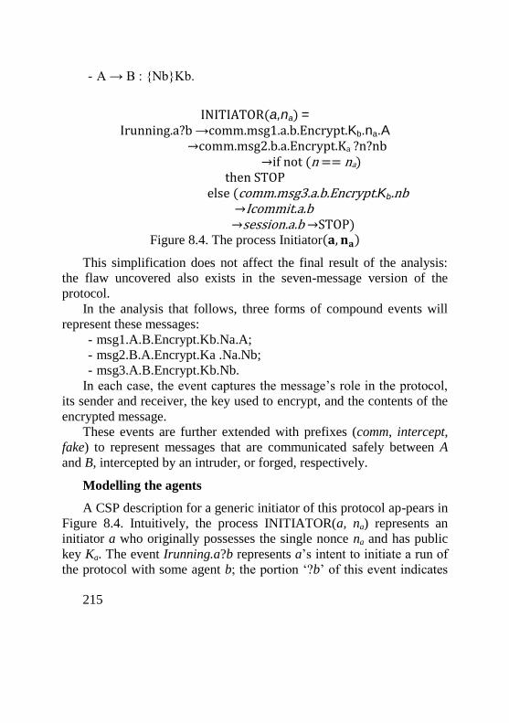
215

- A → B : {Nb}Kb.

INITIATOR(a,na) = Irunning.a?b →comm.msg1.a.b.Encrypt.Kb.na.A →comm.msg2.b.a.Encrypt.Ka ?n?nb

→if not (n == na) then STOP

else (comm.msg3.a.b.Encrypt.Kb.nb →Icommit.a.b

→session.a.b →STOP) Figure 8.4. The process Initiator(𝐚, 𝐧𝐚)

This simplification does not affect the final result of the analysis:

the flaw uncovered also exists in the seven-message version of the

protocol.

In the analysis that follows, three forms of compound events will

represent these messages:

- msg1.A.B.Encrypt.Kb.Na.A;

- msg2.B.A.Encrypt.Ka .Na.Nb;

- msg3.A.B.Encrypt.Kb.Nb.

In each case, the event captures the message’s role in the protocol,

its sender and receiver, the key used to encrypt, and the contents of the

encrypted message.

These events are further extended with prefixes (comm, intercept,

fake) to represent messages that are communicated safely between A

and B, intercepted by an intruder, or forged, respectively.

Modelling the agents

A CSP description for a generic initiator of this protocol ap-pears in

Figure 8.4. Intuitively, the process INITIATOR(a, na) represents an

initiator a who originally possesses the single nonce na and has public

key Ka. The event Irunning.a?b represents a’s intent to initiate a run of

the protocol with some agent b; the portion ‘?b’ of this event indicates

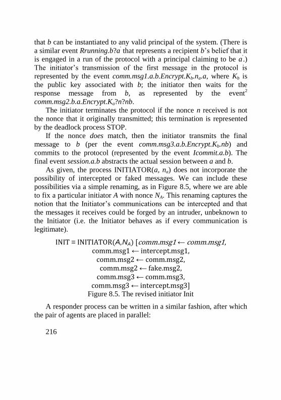
216

that b can be instantiated to any valid principal of the system. (There is

a similar event Rrunning.b?a' that represents a recipient b’s belief that it

is engaged in a run of the protocol with a principal claiming to be a'.)

The initiator’s transmission of the first message in the protocol is

represented by the event comm.msg1.a.b.Encrypt.Kb.na.a, where Kb is

the public key associated with b; the initiator then waits for the

response message from b, as represented by the event2

comm.msg2.b.a.Encrypt.Ka?n?nb.

The initiator terminates the protocol if the nonce n received is not

the nonce that it originally transmitted; this termination is represented

by the deadlock process STOP.

If the nonce does match, then the initiator transmits the final

message to b (per the event comm.msg3.a.b.Encrypt.Kb.nb) and

commits to the protocol (represented by the event Icommit.a.b). The

final event session.a.b abstracts the actual session between a and b.

As given, the process INITIATOR(a, na) does not incorporate the

possibility of intercepted or faked messages. We can include these

possibilities via a simple renaming, as in Figure 8.5, where we are able

to fix a particular initiator A with nonce NA. This renaming captures the

notion that the Initiator’s communications can be intercepted and that

the messages it receives could be forged by an intruder, unbeknown to

the Initiator (i.e. the Initiator behaves as if every communication is

legitimate).

INIT = INITIATOR(A,NA) [comm.msg1 ← comm.msg1, comm.msg1 ← intercept.msg1,

comm.msg2 ← comm.msg2, comm.msg2 ← fake.msg2,

comm.msg3 ← comm.msg3, comm.msg3 ← intercept.msg3]

Figure 8.5. The revised initiator Init

A responder process can be written in a similar fashion, after which

the pair of agents are placed in parallel:

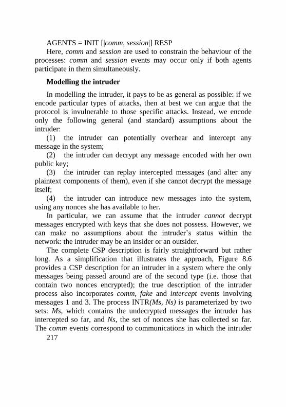
217

AGENTS = INIT [|comm, session|] RESP

Here, comm and session are used to constrain the behaviour of the

processes: comm and session events may occur only if both agents

participate in them simultaneously.

Modelling the intruder

In modelling the intruder, it pays to be as general as possible: if we

encode particular types of attacks, then at best we can argue that the

protocol is invulnerable to those specific attacks. Instead, we encode

only the following general (and standard) assumptions about the

intruder:

(1) the intruder can potentially overhear and intercept any

message in the system;

(2) the intruder can decrypt any message encoded with her own

public key;

(3) the intruder can replay intercepted messages (and alter any

plaintext components of them), even if she cannot decrypt the message

itself;

(4) the intruder can introduce new messages into the system,

using any nonces she has available to her.

In particular, we can assume that the intruder cannot decrypt

messages encrypted with keys that she does not possess. However, we

can make no assumptions about the intruder’s status within the

network: the intruder may be an insider or an outsider.

The complete CSP description is fairly straightforward but rather

long. As a simplification that illustrates the approach, Figure 8.6

provides a CSP description for an intruder in a system where the only

messages being passed around are of the second type (i.e. those that

contain two nonces encrypted); the true description of the intruder

process also incorporates comm, fake and intercept events involving

messages 1 and 3. The process INTR(Ms, Ns) is parameterized by two

sets: Ms, which contains the undecrypted messages the intruder has

intercepted so far, and Ns, the set of nonces she has collected so far.

The comm events correspond to communications in which the intruder

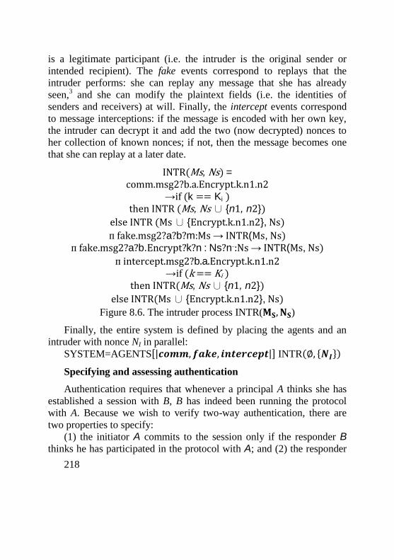
218

is a legitimate participant (i.e. the intruder is the original sender or

intended recipient). The fake events correspond to replays that the

intruder performs: she can replay any message that she has already

seen,3 and she can modify the plaintext fields (i.e. the identities of

senders and receivers) at will. Finally, the intercept events correspond

to message interceptions: if the message is encoded with her own key,

the intruder can decrypt it and add the two (now decrypted) nonces to

her collection of known nonces; if not, then the message becomes one

that she can replay at a later date.

INTR(Ms, Ns) = comm.msg2?b.a.Encrypt.k.n1.n2

→if (k == Ki ) then INTR (Ms, Ns ∪ {n1, n2})

else INTR (Ms ∪ {Encrypt.k.n1.n2}, Ns)

ᴨ fake.msg2?a?b?m:Ms → INTR(Ms, Ns) ᴨ fake.msg2?a?b.Encrypt?k?n : Ns?n

_:Ns → INTR(Ms, Ns)

ᴨ intercept.msg2?b.a.Encrypt.k.n1.n2 →if (k == Ki )

then INTR(Ms, Ns ∪ {n1, n2})

else INTR(Ms ∪ {Encrypt.k.n1.n2}, Ns)

Figure 8.6. The intruder process INTR(𝐌𝐒, 𝐍𝐒)

Finally, the entire system is defined by placing the agents and an

intruder with nonce NI in parallel:

SYSTEM=AGENTS[|𝒄𝒐𝒎𝒎, 𝒇𝒂𝒌𝒆, 𝒊𝒏𝒕𝒆𝒓𝒄𝒆𝒑𝒕|] INTR(∅, {𝑵𝑰})

Specifying and assessing authentication

Authentication requires that whenever a principal A thinks she has

established a session with B, B has indeed been running the protocol

with A. Because we wish to verify two-way authentication, there are

two properties to specify:

(1) the initiator A commits to the session only if the responder B

thinks he has participated in the protocol with A; and (2) the responder

219

B commits to the session only if the initiator A thinks she has

participated in the protocol with B.

These two properties can be expressed in CSP as the processes RA

(receiver authentication) and IA (initiator authentication):

RA = Rrunning.A.B → Icommit.A.B → RA

IA = Irunning.A.B → Rcommit.A.B → IA

To verify that the authentication properties hold, it suffices to

perform the following two refinement checks:

RA SYSTEM \ (∑ − {Rrunning.A.B, Icommit.A.B})

IA SYSTEM \ (∑ − {Irunning.A,B, Rcommit.A.B})

That is, if every trace of SYSTEM (with all events other than

Rrunning.A.B and Icommit.A.B hidden) is also a trace of RA, then the

property RA is guaranteed to hold (and similarly for the property IA).

It turns out that the first refinement check succeeds, but the second

check fails: there are traces of SYSTEM in which the event Rcommit.A.B

occurs without a preceding Irunning.A.B event. For example, SYSTEM

can perform the can the following sequence of events:

Irunning.A.I (1)

intercept.msg1.A.I.Encrypt.KI .NA.A (2)

fake.msg1.A.B.Encrypt.KB.NA.A (3)

Rrunning.A.B (4)

intercept.msg2.B.A.Encrypt.KA.NA.NB (5)

fake.msg2.I.A.Encrypt.KA.NA.NB (6)

intercept.msg3.A.I.Encrypt.KI .NB (7)

fake.msg3.A.B.Encrypt.KB.NB (8)

Rcommit.A.B (9)

The existence of this trace highlights a potential ‘man in the

middle’ attack, whereby the intruder participates as a legitimate

recipient in one run of the protocol with A (the events in lines (1)–(2)

and (6)–(7)) while impersonating A in a second run of the protocol with

B (lines (3)–(5) and (8)–(9)). Ultimately, B commits to a session with

A, despite the fact that A never even attempted to interact with B.

220

8.5 Associating keys and principals

Up until now, we have taken for granted the association between

principals and keys. Correctly making this association is crucial,

particularly when using a PKI. Associating keys with principals

typically depends on two components.

(1) Certification authorities: principals who are recog-nized as

having the authority to vouch for the correct-ness of the associations

between keys and principals.

(2) Certificates: data structures that associate keys with

principals. They are digitally signed by certification authorities to

preserve the integrity of the cryptographic information.

Certificates are much like driver’s licenses and certification

authorities are like the network of authorities who issue those licenses.

Chief among standards for public-key authentication services is the

X.509 standard [8].

Figure 8.7 contains an example of a very simple multiple

certification-authority (MCA) network, where principal CA1 is the

certification authority for principal A, CA2 is the certification authority

for principal B, and CA1 has a certificate for CA2. In this example,

using the notation of X.509, the following certificates exist.

- CA1⟨⟨𝑪𝑨𝟐⟩⟩: a certificate digitally signed with CA1’s private key

certifying that key CA2p is CA2’s public key. The integrity of this

certificate is checked using CA1’s public key CA1p;

- CA2⟨⟨𝑩⟩⟩: a certificate digitally signed with CA2’s private key

certifying that key Bp is B’s public key. The integrity of this

certificate is checked using CA2’s public key CA2p.

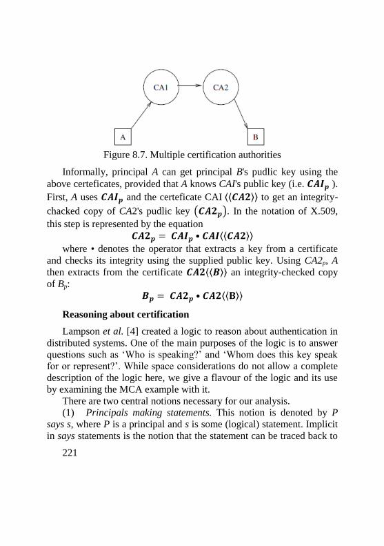
221

Figure 8.7. Multiple certification authorities

Informally, principal A can get principal B's pudlic key using the

above certeficates, provided that A knows CAI's public key (i.e. 𝑪𝑨𝑰𝒑 ).

First, A uses 𝑪𝑨𝑰𝒑 and the certeficate CAI ⟨⟨𝑪𝑨𝟐⟩⟩ to get an integrity-

chacked copy of CA2's pudlic key (𝑪𝑨𝟐𝒑). In the notation of X.509,

this step is represented by the equation

𝑪𝑨𝟐𝒑 = 𝑪𝑨𝑰𝒑 • 𝑪𝑨𝑰⟨⟨𝑪𝑨𝟐⟩⟩

where • denotes the operator that extracts a key from a certificate

and checks its integrity using the supplied public key. Using CA2p, A

then extracts from the certificate 𝑪𝑨𝟐⟨⟨𝑩⟩⟩ an integrity-checked copy

of Bp:

𝑩𝒑 = 𝑪𝑨𝟐𝒑 • 𝑪𝑨𝟐⟨⟨𝐁⟩⟩

Reasoning about certification

Lampson et al. [4] created a logic to reason about authentication in

distributed systems. One of the main purposes of the logic is to answer

questions such as ‘Who is speaking?’ and ‘Whom does this key speak

for or represent?’. While space considerations do not allow a complete

description of the logic here, we give a flavour of the logic and its use

by examining the MCA example with it.

There are two central notions necessary for our analysis.

(1) Principals making statements. This notion is denoted by P

says s, where P is a principal and s is some (logical) statement. Implicit

in says statements is the notion that the statement can be traced back to

222

some digitally signed statement. Principals can be people, machines,

operating systems or cryptographic keys.

(2) Principals speaking for principals. The notion of principal P

speaking for principal Q is denoted by P ⇒ Q. A common idiom is Pp

⇒ P , which indicates that P ’s public key Pp speaks for P : statements

that are digitally signed using Pp will be inferred to be statements made

by P.

The logic is defined by approximately 19 axioms, including the

following handoff axiom:

(P says (Q ⇒ P)) ⊃ (Q ⇒ P).

This handoff axiom says that whenever a principal P states that

another principal Q speaks on P ’s behalf, then Q does speak on P ’s

behalf. Related to this axiom is the property

(P ⇒ Q) ⊃ ((P says s) ⊃ (Q says s)).

This property—derivable from the logic’s axioms—states that

whenever a principal P speaks for Q and makes a statement s, it is safe

to behave as if Q made the statement s.

Analysis of the MCA example

Returning to the example of Figure 8.7, it was shown how this logic

helps us to reason about the certificates and the implicit trust

assumptions that underlie A’s trust in Bp as B’s public key. That is, we

are able to isolate sufficient assumptions under which A can conclude

that Bp ⇒ B.

It turns out that the following five assumptions are sufficient for

concluding Bp ⇒ B.

(1) CA1p ⇒ CA1. A knows the public key of its certification

authority (i.e. from A’s perspective, the key CA1p speaks for CA1).

(2) CA1p says (CA2p ⇒ CA2). CA1’s public key CA1p is used to

verify the validity of the certificate CA1⟨⟨𝑪𝑨𝟐⟩⟩. (3) CA2p says (Bp ⇒ B). Similarly, the key CA2p is used to verify

the certificate CA2⟨⟨𝑩⟩⟩. (4) CA1 ⇒ CA2. A trusts its certificate authority to speak for other

223

certificate authorities (CA2 in this case).

(5) CA2 ⇒ B. A knows that B’s certificate authority is CA2.

The proof of 𝑩𝒑⇒ 𝑩 from these assumptions is straightforward.

From the derived property (𝑷 ⇒ 𝐐) ⊃ ((𝐏 𝐬𝐚𝐲𝐬 𝐬) ⊃ (𝐐 𝐬𝐚𝐲𝐬 𝐬)) and

assumptions (1) and (2), we can deduce that CAI says (𝑪𝑨𝟐𝒑 ⇒ 𝑪𝑨𝟐).

Likewise, we can then use assumption (4) to deduce that

𝑪𝑨𝟐 𝒔𝒂𝒚𝒔 (𝑪𝑨𝟐𝒑 ⇒ 𝑪𝑨𝟐).

From the handoff axiom, we get that 𝑪𝑨𝟐𝒑 ⇒ 𝑪𝑨𝟐. At this point,

the certificate for B in assumption (3) allow us to conclude that

𝑪𝑨𝟐 𝒔𝒂𝒚𝒔 (𝑩𝒑⇒ 𝑩). Another application of the derived property, this

time using assumption (5), lets us deduce that 𝑩 𝒔𝒂𝒚𝒔 (𝑩𝒑⇒ 𝑩).

Finally, the handoff axiom lets us conclude that (𝑩𝒑⇒ 𝑩), which was

our original goal. The value of this analysis is twofold: (1) it makes

explicit the trust assumptions being made, and (2) it assures a consistent

treatment of certificates and assumptions about certification authorities.

8.6 Conclusions

In this chapter there is no attempt to give an exhaustive description

of the applications of formal methods to the problem of assuring

security: we have examined only a single session-based protocol,

designed to provide mutual authentication using a PKI. In particular,

we have ignored shared-key cryptographic systems as well as store-

and-forward security (e.g., secure electronic mail).

Instead, we focused on a single protocol and sketched how multiple

logical systems and formal models can provide insight into security

issues from a variety of viewpoints. The choice of a particular

formalism is driven in part by the properties one wishes to prove and

also by the tools available. Both the BAN logic and the authentication

of logic of are special-purpose modal logics, specifically designed to

support reasoning about freshness and trust. They focus attention on

what principals must be prepared to accept and to believe in order to

trust in the correctness of a protocol. In contrast, the process algebra

224

CSP is a general-purpose language for describing and reasoning about

the behaviour of concurrent systems. For this reason, it is well suited

for reasoning about the high-level interactions and events that may

occur during a run of a protocol.

These analyses demonstrate the subtlety of security properties and

the importance of having rigorous methods for assessing the security of

a system. Security properties are affected by timing and timeliness

(e.g., present versus past runs of a protocol), trust (or lack thereof) in

various principals and authorities, and cryptographic properties.

Furthermore, there are nuances that arise between different levels of

abstraction. The value of these formal methods is that they help in the

detection of weaknesses and possible attacks, as well as making explicit

any necessary assumptions that have been made.

Finally, the methods described in this chapter are all accessible to

engineers with an understanding of predicate logic. The specialized

logics can be embedded into theorem provers: [15] describes the

embedding of a BAN-like logic into the HOL theorem prover [16].

Likewise, there are tools such as Lowe’s Casper [17] that automatically

translate abstract descriptions of security protocols into process-

algebraic descriptions that can be analysed with model checkers.

Advancement questions

1. How can we use the formal methods to analyse protocol?

2. What is the BAN belief logic?

3. What does the security properties describe?

4. What do the key-distribution protocols enable?

5. What is the Needham–Schroeder protocol is designed for?

6. What do the CSP and CCS process algebras provide?

7. What the components the associating keys with principals

depends on?

8. What are the main principals of the modelling the protocol’s

messages?

225

9. What are the main principals of the modelling the intruder?

10. What are the main principals of the specifying and assessing

the authentication?

REFERENCES

[1] Susan Older Formal Methods for Assuring Security of

Protocols / Susan Older, Shiu-Kai Chin // Computer Journal. – 2002. -

Vol. 45, Issue 1. - Pp. 46-54.

[2] Needham, R. Using encryption for authentication in large

networks of computers / Needham, R. and Schroeder, M. - Commun.

ACM 1978, 21. - pp 993-999.

[3] Burroughs M. A Logic of Authentication / Burroughs M.

Abadi M. and Needham R. // Report 39, Digital Equipment Corporation

Systems Research Center. - Palo Alto, CA, February 1989.

[4] Lampson B. Authentication in distributed systems: theory and

practice / Lampson B. Abadi, M. Burroughs M. and Wobber E.// ACM

Trans. Comput. Syst., 10. 1992. - pp 265-310.

[5] Hoare C. A. R. Communicating Sequential Processes (.Series

in Computer Science) / Hoare, C. A. R. - Prentice-Hall. London, 1985.

[6] Menzies A. J. Handbook of Applied Cryptography / Menzies

A. J. von Oorschot P. C. and Vanstone S. A. - CRC Press, New York,

1996.

[7] Handbook of Applied Cryptography / Menzies, A. J., von

Oorschot, P. C. and Vanstone S. A. - CRC Press, New York, 1996.

[8] Information Technology—Open Systems Interconnection—

The Directory: Authentication Framework: ISO/EC 9594-8, 1995. -

ISO Standart

[9] Gong L. Reasoning about belief in cryptographic protocols/

Gong L. Needham R. and Yahalom R. // In Proc. 1990 IEEEComput.

226

Soc. Symp. on Research in Security and Privacy, Oakland, CA, May. -

1990. - pp. 234-248.

[10] van Oorschot P. Extending cryptographic logics of belief to

key agreement protocol / van Oorschot P. // In Proc. First ACM Conf

on Computers and Communications Security, Fairfax, VA. - 1993

November. - pp. 232-243.

[11] Roscoe A. W. The Theory and Practice of Concurrency

(Series in Computer Science) / A. W. Roscoe Prentice-Hall, London,

1998.

[12] Milner R. A Calculus of Communicating Systems/ R. Milner

// Springer, Berlin. -1980 . - Vol. 92.

[13] Formal Systems (Europe) Ltd / Failures-Divergence

Refinement: EDR2 User Manual. - Oxford, 1997.

[14] Lowe G. An attack on the Needham-Schroeder public-key

authentication protocol / G. Lowe // Inform. Process. Lett., 56, 1995. -

pp 131-133.

[15] Lowe G. Breaking and fixing the Needham- Schroeder

public-key protocol using fdr / G. Lowe. - Software Concepts Tools,

17, 1996. - pp 93-102.

[16] 15 Schubert T. A mechanized logic for secure key escrow

protocol verification/ T. Schubert and S. Mocas // In Proc. Eighth Int.

Workshop on Higher Order Logic Theorem Proving and Its

Applications. - 1995.

[17] 16 Gordon M. J. C. Introduction to HOL: A Theorem

Proving Environment for Higher Order Logic / M. J. C. Gordon and T.

F. Melham. - Cambridge University Press, Cambridge, 1993.

[18] 17 Lowe G. Casper: a compiler for the analysis of security

protocols / G. Lowe // J. Comput. Security, 6, 1998. - pp 53-84.

227

CHAPTER 9. FORMAL METHODS FOR THE ANALYSIS

OF SECURITY PROTOCOLS

Content of the CHAPTER 9

Soundness of Formal Encryption

Relating Symbolic and Computational cryptography has attracted

the interest of the research community. Several different directions

have been taken to bridge the gap between the two models: some

extend the existing results by including more primitives; some by

adapting existing results from the passive adversary scenario to the

active adversary scenario; some others by including new primitives

from computational cryptography.

This chapter is one more effort to bridge the gap between these two

communities. Mainly, let us try to bridge two gaps that exist since the

early results of Abadi and Rogaway. The first is the non-existence of

soundness results in the presence of key-cycles. Key-cycles do not

present a problem from the symbolic point of view. One may even

argue that protocols that create messages with encryption cycles may be

avoided and are just result of bad engineering. But, even if our

protocols are restricted to the cases where no cycles are created, no one

can ensure us that an adversary is not able to create cyclic encryptions

and that these would not cause problems. Studying this is part of the

work in this chapter. We can show that it is possible to close this gap

but for that the use of new definitions of security is needed.

The second gap is to be closen is to extend the original Abadi and

Rogaway result when the encryption scheme used provides less security

guarantees. The encryption scheme used in their original result is very

strong and arguably impossible to realise in many contexts. The aim is

to relax such conditions by allowing the use of weaker encryption

schemes but still achieving similar soundness results. It will allow

encryption schemes that reveal the length of the encrypted plaintext.

Let us study this particular example and then show a uniform

228

framework with which it will be able to characterise a large family of

encryption schemes.

9.1 The Abadi-Rogaway Soundness Theorem

The main definitions and results of Abadi and Rogaway’s original

work are briefly summarised [4, 2]. In particular, let us start presenting

the formal model, then describe the computational model, and then

introduce the notion of soundness. Furthermore, let us introduce the

notion of completeness, which can be viewed as the counter-point to

soundness.

The Formal Model

In this model, messages (or expressions) are defined at a very high

level of abstraction. The simplest expressions are symbols for atomic

keys and bit-strings. More complex expressions are created from

simpler ones via encryption and concatenation, which are defined as

abstract, ‘black-box’ constructors.

Definition 9.1 (Symmetric Expressions). Let Keys = {𝐊𝟏; 𝐊𝟐; 𝐊𝟑;… } be an infinite discrete set of symbols, called the set of

symmetric keys. Let Blocks be a finite subset of {𝟎, 𝟏}∗. We define the

set of expressions, Exp, by the grammar:

Exp ::= Keys | Blocks | (Exp; Exp) | {𝐄𝐱𝐩}𝐊𝐞𝐲𝐬

Let Enc ::= {𝐄𝐱𝐩}𝐊𝐞𝐲𝐬. We will denote by Keys(M) the set of all

keys occurring in M. Expressions of the form {𝑴}𝑲 are called

encryption terms.

Expressions may represent either a single message sent during an

execution of the protocol, or the entire knowledge available to the

adversary. In this second case, the expression contains not only the

messages sent so far, but also any additional knowledge in the

adversary’s possession.

Let us define two formal expressions are indistinguishable to the

adversary. Intuitively, this occurs when the only differences between

the two messages lie within encryption terms that the adversary cannot

decrypt. In order to rigorously define this notion, we first need to

229

formalise when an encryption term is ‘undecryptable’ by the adversary,

which in turn requires us to define the set of keys that the adversary can

learn from an expression.

An expression might contain keys in the clear. The adversary will

learn these keys, and can then use them to decrypt encryption terms of

the expression—which might reveal yet more keys. By repeating this

process, the adversary can learn the set of recoverable decryption keys:

Definition 9.2 (Subexpressions, Visible Subexpressions,

Recoverable Keys, Undecryptable Terms, B-Keys). We define the set

of subexpressions of an expression M, sub (M), as the small-est subset

of expressions containing M such that:

- (M1; M2) ∈ sub (M) M1 ∈ sub (M) and M2 ∈ sub (M), and {𝑴′}𝑲 ∈ sub (M) 𝑴′ ∈ sub (M).

We say that N is a subexpression of M, and denote it by N M, if N ∈

sub (M).

The set of visible subexpressions of a symmetric expression M, vis

(M), is the smallest subset of expressions containing M such that:

- (M1; M2) ∈ vis (M) M1 ∈ vis (M) and M2 ∈ vis (M), and {𝑴′}𝑲 and K ∈ vis (M) 𝑴′ ∈ vis (M).

The recoverable keys of a (symmetric) expression M, R-Keys(M),

are those that an adversary can recover by looking at an expression.

That is, R-Keys(M) = vis (M) Keys(M).

We say that an encryption term {𝑴′}𝑲 ∈ vis (M) is undecryptable in

M if K ∉ R-Keys(M). Among the non-recoverable keys of an expression

M, there is an important subset denoted by B-Keys(M). The set B-

Keys(M) contains those keys which encrypt the outermost

undecryptable terms. Formally, for an expression M, we define B-

Keys(M) as

B-Keys(M)={𝑲 ∈ 𝑲𝒆𝒚𝒔(𝑴) | {𝑴}𝑲 ∈ 𝒗𝒊𝒔 (𝑴) 𝐛𝐮𝐭 𝑲 ∉ 𝑹 −𝑲𝒆𝒚𝒔(𝑴)𝒈 }

Example 9.1. Let M be the following expression

(({𝑸}𝑲𝟔 , {{𝑲𝟕}𝑲𝟏}𝑲𝟒((𝑲𝟐, {({𝟎𝟎𝟏}𝑲𝟑 , {𝑲𝟔}𝑲𝟓)}𝑲𝟓

) , {𝑲𝟓} 𝑲𝟐 )).

230

In this case, Keys(M) = {𝑲𝟏; 𝑲𝟐; 𝑲𝟑; 𝑲𝟒; 𝑲𝟓; 𝑲𝟔; 𝑲𝟕}. The set

of recoverable keys of M is R-Keys(M) ={ 𝑲𝟐; 𝑲𝟓; 𝑲𝟔}, because an

adversary sees the non-encrypted K2, and with that he can decrypt

{ 𝑲𝟓}𝑲𝟐 , hence recovering K5; then, decrypting twice with K5, K6 can

be revealed. We also have that B-Keys(M) = { 𝑲𝟑; 𝑲𝟒}. The formal model allows expressions to contain key cycles:

Definition 9.3 (Key-Cycles). An expression M contains a key-cycle

if it contains encryption terms {𝑴𝟏}𝑲𝟏 , {𝑴𝟐}𝑲𝟐 , … , {𝑴𝒏}𝑲𝒏 (where

{𝑴𝒊}𝑲𝒊denotes the encryption of the message Mi with the key Ki) and

Ki+1 v Mi and K1 v Mn. In this case we say that we have a key-cycle of

length n.

According to our definition, expressions such as {{𝑴}𝑲}𝑲 are not

considered cyclic. The original result of Abadi and Rogaway does not

apply to expressions with key cycles. The aim is to correct this

weaknes.

The AR Equivalence of Formal Expressions

A visible encryption term will appear ‘opaque’ to the adversary if

and only if it is protected by at least one non-recoverable decryption

key. Thus, we can to say that two expressions are equivalent if they

differ only in the contents of their ‘opaque’ encryption terms. To

express this, Abadi and Rogaway define the pattern of an expression

through which equivalence of expressions will be obtained:

Definition 9.4 (Pattern (Classical)). We define the set of patterns,

Pat, by the grammar:

Pat ::= Keys | Blocks | (Pat; Pat) | {𝐏𝐚𝐭}𝐊𝐞𝐲𝐬

The pattern of an expression M, denoted by pattern(M), is derived

from M by replacing each encryption term {𝑴′}𝑲 ∈ vis (M) (where K ∉

= R-Keys(M)) by for two patterns P and Q, P = Q is defined the

following way:

- if P ∈ Blocks ∪ Keys, then P = Q iff P and Q are identical;

- if P is of the form, then P = Q iff Q is of the form;

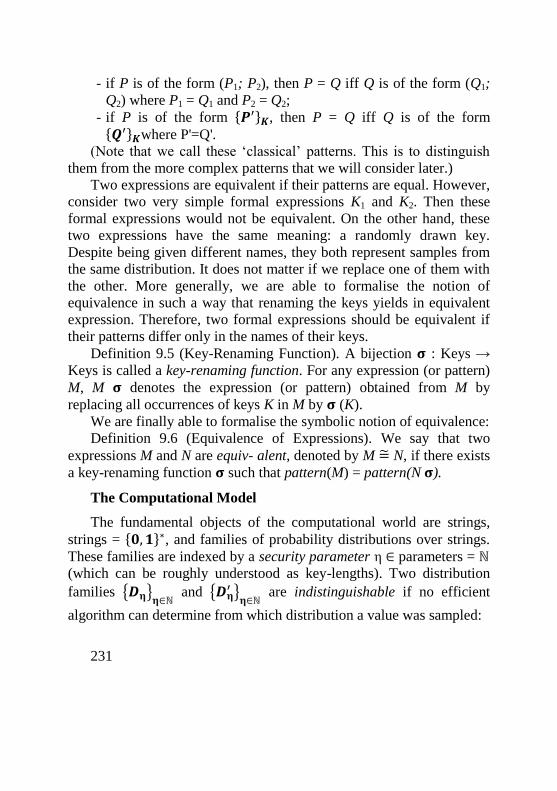
231

- if P is of the form (P1; P2), then P = Q iff Q is of the form (Q1;

Q2) where P1 = Q1 and P2 = Q2;

- if P is of the form {𝑷′}𝑲, then P = Q iff Q is of the form {𝑸′}𝑲where P'=Q'.

(Note that we call these ‘classical’ patterns. This is to distinguish

them from the more complex patterns that we will consider later.)

Two expressions are equivalent if their patterns are equal. However,

consider two very simple formal expressions K1 and K2. Then these

formal expressions would not be equivalent. On the other hand, these

two expressions have the same meaning: a randomly drawn key.

Despite being given different names, they both represent samples from

the same distribution. It does not matter if we replace one of them with

the other. More generally, we are able to formalise the notion of

equivalence in such a way that renaming the keys yields in equivalent

expression. Therefore, two formal expressions should be equivalent if

their patterns differ only in the names of their keys.

Definition 9.5 (Key-Renaming Function). A bijection 𝛔 : Keys →

Keys is called a key-renaming function. For any expression (or pattern)

M, M 𝛔 denotes the expression (or pattern) obtained from M by

replacing all occurrences of keys K in M by 𝛔 (K).

We are finally able to formalise the symbolic notion of equivalence:

Definition 9.6 (Equivalence of Expressions). We say that two

expressions M and N are equiv- alent, denoted by M =̃ N, if there exists

a key-renaming function 𝛔 such that pattern(M) = pattern(N 𝛔).

The Computational Model

The fundamental objects of the computational world are strings,

strings = {𝟎, 𝟏}∗, and families of probability distributions over strings.

These families are indexed by a security parameter η ∈ parameters = ℕ

(which can be roughly understood as key-lengths). Two distribution

families {𝑫𝛈}𝛈∈ℕ and {𝑫𝛈

′ }𝛈∈ℕ

are indistinguishable if no efficient

algorithm can determine from which distribution a value was sampled:

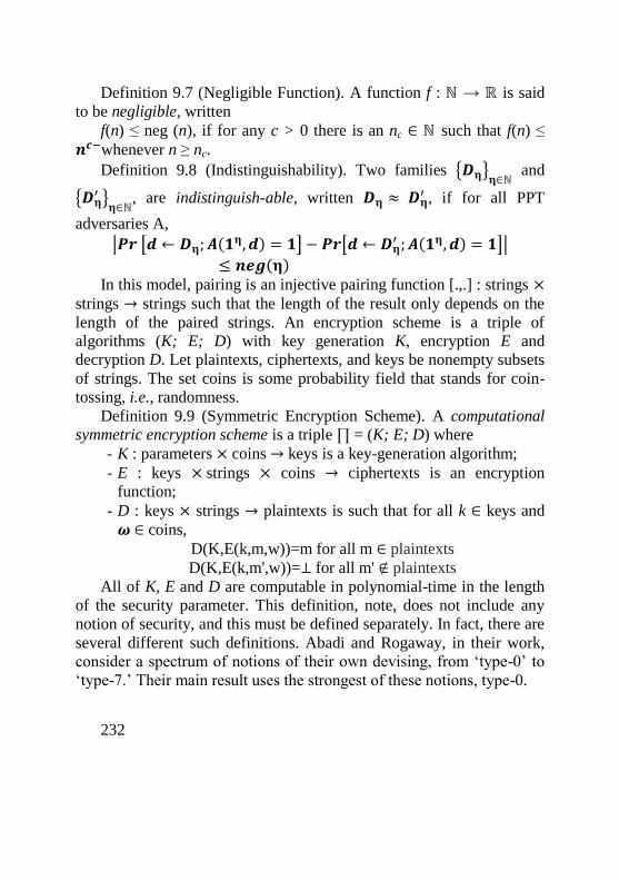
232

Definition 9.7 (Negligible Function). A function f : ℕ → ℝ is said

to be negligible, written

f(n) ≤ neg (n), if for any c > 0 there is an nc ∈ ℕ such that f(n) ≤

𝒏𝒄−whenever n ≥ nc.

Definition 9.8 (Indistinguishability). Two families {𝑫𝛈}𝛈∈ℕ and

{𝑫𝛈′ }𝛈∈ℕ

, are indistinguish-able, written 𝑫𝛈 ≈ 𝑫𝛈′ , if for all PPT

adversaries A,

|𝑷𝒓 [𝒅 ← 𝑫𝛈; 𝑨(𝟏𝛈, 𝒅) = 𝟏] − 𝑷𝒓[𝒅 ← 𝑫𝛈

′ ; 𝑨(𝟏𝛈, 𝒅) = 𝟏]|

≤ 𝒏𝒆𝒈(𝛈) In this model, pairing is an injective pairing function [.,.] : strings ×

strings → strings such that the length of the result only depends on the

length of the paired strings. An encryption scheme is a triple of

algorithms (K; E; D) with key generation K, encryption E and

decryption D. Let plaintexts, ciphertexts, and keys be nonempty subsets

of strings. The set coins is some probability field that stands for coin-

tossing, i.e., randomness.

Definition 9.9 (Symmetric Encryption Scheme). A computational

symmetric encryption scheme is a triple ∏ = (K; E; D) where

- K : parameters × coins → keys is a key-generation algorithm;

- E : keys × strings × coins → ciphertexts is an encryption

function;

- D : keys × strings → plaintexts is such that for all k ∈ keys and

𝝎 ∈ coins,

D(K,E(k,m,w))=m for all m ∈ plaintexts

D(K,E(k,m',w))=⊥ for all m' ∉ plaintexts

All of K, E and D are computable in polynomial-time in the length

of the security parameter. This definition, note, does not include any

notion of security, and this must be defined separately. In fact, there are

several different such definitions. Abadi and Rogaway, in their work,

consider a spectrum of notions of their own devising, from ‘type-0’ to

‘type-7.’ Their main result uses the strongest of these notions, type-0.

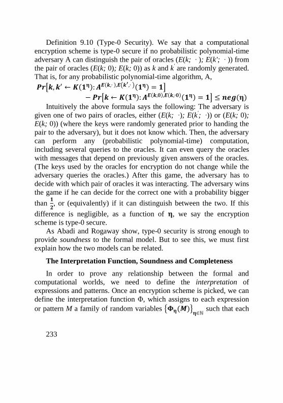
233

Definition 9.10 (Type-0 Security). We say that a computational

encryption scheme is type-0 secure if no probabilistic polynomial-time

adversary A can distinguish the pair of oracles (E(k; ∙ ); E(k'; ∙ )) from

the pair of oracles (E(k; 0); E(k; 0)) as k and k' are randomly generated.

That is, for any probabilistic polynomial-time algorithm, A,

𝑷𝒓[𝒌, 𝒌′ ← 𝑲(𝟏𝛈): 𝑨𝑬(𝒌,∙ ),𝑬(𝒌′,∙ )(𝟏𝛈) = 𝟏]

− 𝑷𝒓[𝒌 ← 𝑲(𝟏𝛈): 𝑨𝑬(𝒌,𝟎),𝑬(𝒌,∙𝟎)(𝟏𝛈) = 𝟏] ≤ 𝒏𝒆𝒈(𝛈) Intuitively the above formula says the following: The adversary is

given one of two pairs of oracles, either (E(k; ∙); E(k'; ∙)) or (E(k; 0);

E(k; 0)) (where the keys were randomly generated prior to handing the

pair to the adversary), but it does not know which. Then, the adversary

can perform any (probabilistic polynomial-time) computation,

including several queries to the oracles. It can even query the oracles

with messages that depend on previously given answers of the oracles.

(The keys used by the oracles for encryption do not change while the

adversary queries the oracles.) After this game, the adversary has to

decide with which pair of oracles it was interacting. The adversary wins

the game if he can decide for the correct one with a probability bigger

than 𝟏

𝟐, or (equivalently) if it can distinguish between the two. If this

difference is negligible, as a function of 𝛈, we say the encryption

scheme is type-0 secure.

As Abadi and Rogaway show, type-0 security is strong enough to

provide soundness to the formal model. But to see this, we must first

explain how the two models can be related.

The Interpretation Function, Soundness and Completeness

In order to prove any relationship between the formal and

computational worlds, we need to define the interpretation of

expressions and patterns. Once an encryption scheme is picked, we can

define the interpretation function Φ, which assigns to each expression

or pattern M a family of random variables {𝚽𝛈(𝑴)}𝛈∈ℕ such that each

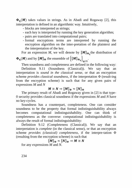
234

𝚽𝛈(𝑴) takes values in strings. As in Abadi and Rogaway [2], this

interpretation is defined in an algorithmic way. Intuitively,

- blocks are interpreted as strings;

- each key is interpreted by running the key generation algorithm;

- pairs are translated into computational pairs;

- formal encryptions terms are interpreted by running the

encryption algorithm on the inter-pretation of the plaintext and

the interpretation of the key.

For an expression M, we will denote by ⟦𝑴⟧𝚽𝛈the distribution of

𝚽𝛈(𝑴) and by ⟦𝑴⟧𝚽 the ensemble of {⟦𝑴⟧𝚽𝛈}𝛈∈ℕ.

Then soundness and completeness are defined in the following way:

Definition 9.11 (Soundness (Classical)). We say that an

interpretation is sound in the classical sense, or that an encryption

scheme provides classical soundness, if the interpretation Φ (result-ing

from the encryption scheme) is such that for any given pairs of

expressions M and N

𝑴 ≅ 𝑵 ⇒ ⟦𝑴⟧𝚽 ≈ ⟦𝑵⟧𝚽 The primary result of Abadi and Rogaway given in [2] is that type-

0 security provides classical soundness if the expressions M and N have

no key-cycles.

Soundness has a counterpart, completeness. One can consider

soundness to be the property that formal indistinguishability always

becomes computational indistinguishability. One can think of

completeness as the converse: computational indistinguishability is

always the result of formal indistinguishability:

Definition 9.12 (Completeness (Classical)). We say that an

interpretation is complete (in the classical sense), or that an encryption

scheme provides (classical) completeness, if the interpre-tation Φ

(resulting from the encryption scheme) is such that

⟦𝑴⟧𝚽 ≈ ⟦𝑵⟧𝚽 ⇒𝑴 ≅ 𝑵 for any expressions M and N.

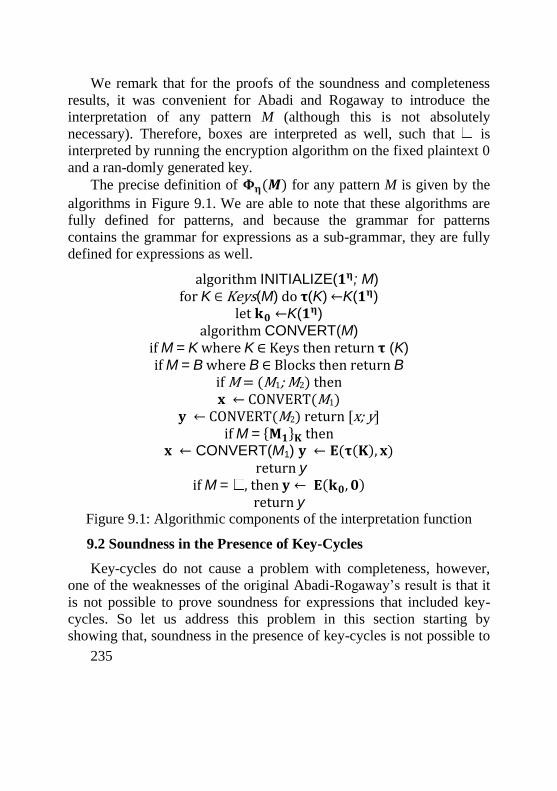
235

We remark that for the proofs of the soundness and completeness

results, it was convenient for Abadi and Rogaway to introduce the

interpretation of any pattern M (although this is not absolutely

necessary). Therefore, boxes are interpreted as well, such that is

interpreted by running the encryption algorithm on the fixed plaintext 0

and a ran-domly generated key.

The precise definition of 𝚽𝛈(𝑴) for any pattern M is given by the

algorithms in Figure 9.1. We are able to note that these algorithms are

fully defined for patterns, and because the grammar for patterns

contains the grammar for expressions as a sub-grammar, they are fully

defined for expressions as well.

algorithm INITIALIZE(𝟏𝛈; M) for K ∈ Keys(M) do 𝛕(K) ←K(𝟏𝛈)

let 𝐤𝟎 ←K(𝟏𝛈) algorithm CONVERT(M)

if M = K where K ∈ Keys then return 𝛕 (K) if M = B where B ∈ Blocks then return B

if M = (M1; M2) then 𝐱 ← CONVERT(M1)

𝐲 ← CONVERT(M2) return [x; y] if M = {𝐌𝟏}𝐊 then

𝐱 ← CONVERT(M1) 𝐲 ← 𝐄(𝛕(𝐊), 𝐱) return y

if M = , then 𝐲 ← 𝐄(𝐤𝟎, 𝟎) return y

Figure 9.1: Algorithmic components of the interpretation function

9.2 Soundness in the Presence of Key-Cycles

Key-cycles do not cause a problem with completeness, however,

one of the weaknesses of the original Abadi-Rogaway’s result is that it

is not possible to prove soundness for expressions that included key-

cycles. So let us address this problem in this section starting by

showing that, soundness in the presence of key-cycles is not possible to

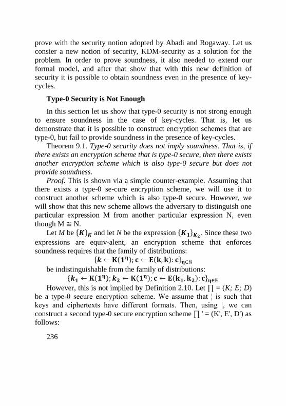
236

prove with the security notion adopted by Abadi and Rogaway. Let us

consier a new notion of security, KDM-security as a solution for the

problem. In order to prove soundness, it also needed to extend our

formal model, and after that show that with this new definition of

security it is possible to obtain soundness even in the presence of key-

cycles.

Type-0 Security is Not Enough

In this section let us show that type-0 security is not strong enough

to ensure soundness in the case of key-cycles. That is, let us

demonstrate that it is possible to construct encryption schemes that are

type-0, but fail to provide soundness in the presence of key-cycles.

Theorem 9.1. Type-0 security does not imply soundness. That is, if

there exists an encryption scheme that is type-0 secure, then there exists

another encryption scheme which is also type-0 secure but does not

provide soundness.

Proof. This is shown via a simple counter-example. Assuming that

there exists a type-0 se-cure encryption scheme, we will use it to

construct another scheme which is also type-0 secure. However, we

will show that this new scheme allows the adversary to distinguish one

particular expression M from another particular expression N, even

though M ≅ N.

Let M be {𝑲}𝑲 and let N be the expression {𝑲𝟏}𝑲𝟐. Since these two

expressions are equiv-alent, an encryption scheme that enforces

soundness requires that the family of distributions: {𝒌 ← 𝐊(𝟏𝛈); 𝐜 ← 𝐄(𝐤, 𝐤): 𝐜}𝛈∈ℕ

be indistinguishable from the family of distributions:

{𝒌𝟏 ← 𝐊(𝟏𝛈); 𝒌𝟐 ← 𝐊(𝟏

𝛈); 𝐜 ← 𝐄(𝐤𝟏, 𝐤𝟐): 𝐜}𝛈∈ℕ

However, this is not implied by Definition 2.10. Let ∏ = (K; E; D)

be a type-0 secure encryption scheme. We assume that ¦ is such that

keys and ciphertexts have different formats. Then, using ¦, we can

construct a second type-0 secure encryption scheme ∏ ' = (K', E', D') as

follows:

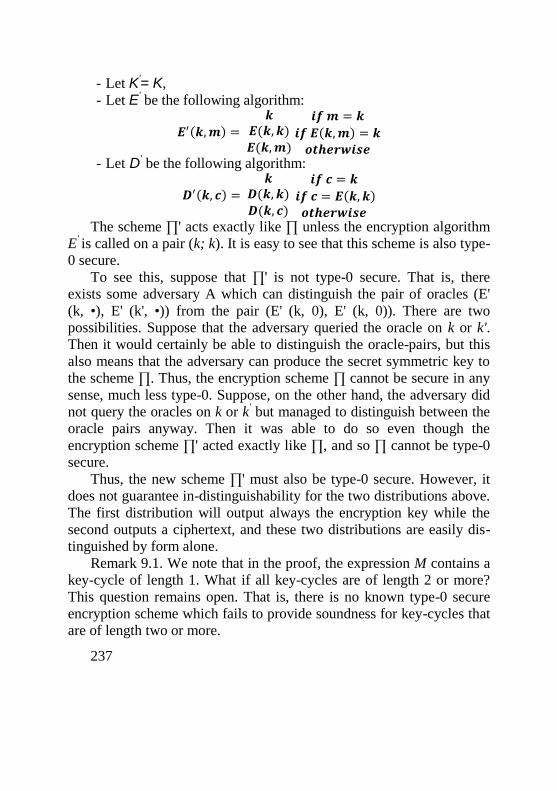
237

- Let K'= K, - Let E'

be the following algorithm:

𝑬′(𝒌,𝒎) =

𝒌𝑬(𝒌, 𝒌)

𝑬(𝒌,𝒎) 𝒊𝒇 𝒎 = 𝒌

𝒊𝒇 𝑬(𝒌,𝒎) = 𝒌𝒐𝒕𝒉𝒆𝒓𝒘𝒊𝒔𝒆

- Let D' be the following algorithm:

𝑫′(𝒌, 𝒄) =

𝒌𝑫(𝒌, 𝒌)

𝑫(𝒌, 𝒄) 𝒊𝒇 𝒄 = 𝒌

𝒊𝒇 𝒄 = 𝑬(𝒌, 𝒌)

𝒐𝒕𝒉𝒆𝒓𝒘𝒊𝒔𝒆

The scheme ∏' acts exactly like ∏ unless the encryption algorithm

E' is called on a pair (k; k). It is easy to see that this scheme is also type-

0 secure.

To see this, suppose that ∏' is not type-0 secure. That is, there

exists some adversary A which can distinguish the pair of oracles (E'

(k, •), E' (k', •)) from the pair (E' (k, 0), E' (k, 0)). There are two

possibilities. Suppose that the adversary queried the oracle on k or k'.

Then it would certainly be able to distinguish the oracle-pairs, but this

also means that the adversary can produce the secret symmetric key to

the scheme ∏. Thus, the encryption scheme ∏ cannot be secure in any

sense, much less type-0. Suppose, on the other hand, the adversary did

not query the oracles on k or k' but managed to distinguish between the

oracle pairs anyway. Then it was able to do so even though the

encryption scheme ∏' acted exactly like ∏, and so ∏ cannot be type-0

secure.

Thus, the new scheme ∏' must also be type-0 secure. However, it

does not guarantee in-distinguishability for the two distributions above.

The first distribution will output always the encryption key while the

second outputs a ciphertext, and these two distributions are easily dis-

tinguished by form alone.

Remark 9.1. We note that in the proof, the expression M contains a

key-cycle of length 1. What if all key-cycles are of length 2 or more?

This question remains open. That is, there is no known type-0 secure

encryption scheme which fails to provide soundness for key-cycles that

are of length two or more.

238

Because type-0 encryption implies types 1 through 7, Theorem 9.1

implies that soundness with key-cycles cannot be provided by the

security definitions devised by Abadi and Rogaway. In the next section,

shows that the soundness property can be met with new computational

definitions.

KDM-Security

In the last section, it was shown that the notions of security found in

[4, 2] are not strong enough to enforce soundness in the presence of

key-cycles. However, key-dependent message (KDM) security, which

was introduced by Black et al. [3] (and in a weaker form by Camenisch

and Lysyanskaya [5]), is strong enough to enforce soundness even in

this case.

KDM security both strengthens and weakens type-0 security. Recall

that type-0 security allows the adversary to submit messages to an

oracle which does one of two things:

- it could encrypt the message twice, under two different keys, or it

could encrypt the bit 0 twice, under the same key. An encryption scheme is type-0 secure if no adversary can tell

which of these is being done. For KDM security, however, the game is

slightly different. To over-simplify:

- the oracle in the KDM-security encrypts once, under only one

key; - further, it encrypts either the message, or a string of 0’s of

equivalent length; - however, it is willing to encrypt not just messages from the

adversary, but also (more generally) functions of the secret key. The first two of these differences make KDM security weaker than

type-0 security. Specifically type-0 security conceals both the length of

the plaintext and whether two ciphertext were created using the same

encryption key or different ones. KDM security does not necessarily

conceal either of these things. The last difference, however, is a

significant strengthening. As its name suggests, KDM security remains

239

strong even when the messages depend on the secret key— which, as

Theorem 2.1 shows, is not necessarily true for type-0 security.

To provide the full picture, KDM security is defined in terms of

vectors of keys and functions over these vectors. It is also defined in

terms of oracles 𝑹𝒆𝒂𝒍�̅� and 𝑭𝒂𝒌𝒆�̅� , which work as follows:

- suppose that for a fixed security parameter η ∈ ℕ , a vector of

keys is given �̅� = {𝒌𝒊 ← 𝐊(𝟏𝛈)}𝒊∈ ℕ (In each run of the key-

generation algorithm independent coins are used.) The adversary

can now query the oracles providing them with a pair (j, g),

where j ∈ ℕ and g : 𝒌𝒆𝒚𝒔∞ → {𝟎, 𝟏}∗ is a constant length,

deterministic function:

96. - The oracle 𝑹𝒆𝒂𝒍�̅� when receiving this input returns c ←

𝑬(𝒌𝒋, 𝒈(�̅�)).

97. - The oracle 𝑭𝒂𝒌𝒆�̅� when receiving this same input returns c

← 𝑬(𝒌𝒋, 𝟎|𝒈(�̅�)|).

The challenge facing the adversary is to decide whether it has

interacted with oracle 𝑹𝒆𝒂𝒍�̅� or oracle 𝑭𝒂𝒌𝒆�̅�. Formally:

Definition 9.13 (Symmetric-KDM Security). Let ∏ = (K,E,D) be a

symmetric encryption scheme. Let the two oracles 𝑹𝒆𝒂𝒍�̅� and 𝑭𝒂𝒌𝒆�̅�

be as defined above. We say that the encryption scheme is (symmetric)

KDM-secure if for all PPT adversaries A:

𝐏𝐫[�̅� ← 𝐊(𝟏𝛈): 𝐀𝑹𝒆𝒂𝒍�̅� (𝟏𝛈) = 𝟏]

− 𝐏𝐫[�̅� ← 𝐊(𝟏𝛈): 𝐀𝑭𝒂𝒌𝒆�̅� (𝟏𝛈) = 𝟏] ≤ 𝒏𝒆𝒈(𝛈) Remark 9.2. We note that although all known implementations of

KDM-security are in the random-oracle model, this definition is well-

founded even in the standard model. We also note that this definition is

phrased in terms of indistinguishability. One could also imagine

analogous defini-tions phrased in terms of non-malleability, but an

exploration of those are beyond the scope of this dissertation.

We note that KDM-security implies type-3 security:

Definition 9.14 (Type-3 Security). Let ∏ = (K,E,D) be a symmetric

encryption scheme. We say that the encryption-scheme is type-3 secure

240

if no PPT adversary A can distinguish the oracles 𝑬(𝒌,•) and

𝑬(𝒌; 𝟎|•|) as k is randomly generated, that is, for all PPT adversaries

A:

𝑷𝒓 [𝒌 ← 𝐊(𝟏𝛈): 𝐀𝑬(𝒌,•)] − 𝑷𝒓 [𝒌 ← 𝐊(𝟏𝛈): 𝐀𝑬(𝒌; 𝟎|•|) (𝟏𝛈) = 𝟏]

≤ 𝒏𝒆𝒈(𝛈) In fact, the definition of type-3 encryption is exactly the same as

that for KDM-security, except that the adversary must submit concrete

messages to the encryption oracle instead of functions. But since the

functions submitted in KDM security can be constant function that

always produce a single output, the type-3 security ‘game’ is a special

case of that for KDM security.

On the other hand, KDM security does not attempt to conceal the

length of the plaintext (type-1 security) or that two ciphertexts were

created with the same key (type-2 security). It will be impossible,

therefore, for KDM security to provide soundness in the classical sense

(Defini-tion 2.11). Nonetheless, a weaker form of soundness can be

achieved if the formal model is also weakened slightly.

A New Formal Model

In this section, let us consider a weaker version of the formal

model—one that allows formal en-cryption to leak partial information

about the plaintext and key. Here let us focus on the partial leakage

allowed (in the computational model) by KDM security: the length of

the plaintext, and whether two different ciphertexts were created using

the same key.

To model the leakage of plaintext length, we first need to add the

very concept of ‘length’ to the formal model.

Definition 9.15 (Formal Length). A formal length-function is a

function symbol with fresh letter l satisfying at least the following

identities:

- for all blocks B1 and B2, l (B1) = l (B2) iff |𝑩𝟏| = |𝑩𝟐|; - for all expression M and key-renaming function σ, l (M) = l (M σ)

- if l (M1) = l (N1), l (M2) = l (N2) then l ((M1; M2)) = l ((N1; N2)),

241

and

- if l (M) = l (N), then for all Ki, l ({𝑴}𝑲𝒊)= l ({𝑵}𝑲𝒊).

These are the identities that a formal length function mini-mally has

to satisfy. There may be more. In fact, if only these properties are

assumed, there is no hope to obtain completeness. It follows that for

any key-renaming function σ, and expression M, l (M) = l (M σ).

Given this, it is straightforward to add the required leakage to the

formal model. If patterns represents those aspects of an expression that

can be learned by the adversary, then patterns must now reveal the

plaintext-length and key-names for undecryptable terms:

Definition 9.16 (Pattern (Type-3)). We define the set of patterns,

Pat, by the grammar:

Pat ::= Keys | Blocks | (Pat; Pat) | {𝑷𝒂𝒕}𝑲𝒆𝒚𝒔 | 𝑲𝒆𝒚𝒔,𝒍(𝐄𝐱𝐩)

The type-3 pattern of an expression M, denoted by pattern3(M), is

derived from M by replacing each encryption term {𝑴′}𝑲 ∈

𝒗𝒊𝒔 (𝑴)(𝒘𝒉𝒆𝒓𝒆 𝑲 ∉ 𝑹 − 𝑲𝒆𝒚𝒔 (𝑴))𝒃𝒚 𝑲,𝒍(𝐌′).

Note that the only difference between a type-3 pattern and a

classical pattern is that an unde-cryptable term {𝑴}𝑲becomes 𝑲,𝒍(𝐌)

(i.e. labelled with the key and length) in type-3 patterns instead of

merely in classical patterns.

Our notion of formal equality must be updated as well. For two

patterns P and Q, 𝑷 ≅𝟑 𝑸 is defined the following way:

Definition 9.17 (Formal Equivalence (Type-3)). We first introduce

the relation =3 between patterns:

- if P ∈ Blocks ∪ Keys, then P =3 Q iff P and Q are identical;

- if P is of the form 𝑲,𝒍(𝐌′), then P =3 Q iff Q is of the form

𝑲,𝒍(𝐍′), and l (M') = l (N') in the sense of Definition 2.15;

- if P is of the form (P1; P2), then P =3 Q iff Q is of the form (Q1;

Q2) where P1 =3 Q1 and P2 =3 Q2.;

- if P is of the form {𝑷′}𝑲, then P =3 Q iff Q is of the form {𝑸′}𝑲,

where P ' =3 Q'.

242

With this, we say that expressions M and N are equivalent in the

type-3 sense (writen 𝑴 ≅𝟑 𝑵) if there exists a key-renaming function σ

such that pattern3 (M) =3 pattern3 (Nσ). (Since a key-renaming function

replaces all occurrences of K with σ(K), we note σ, 𝑲,𝒍(𝐌) will

become 𝛔 (𝐊),𝒍(𝑴𝛔)•)

Lastly, the above change to formal equivalence requires that the

notions of soundness and completeness be similarly altered:

Definition 9.18 (Soundness (Type-3)). We say that an interpretation

is type-3 sound, or that an encryption scheme provides soundness in the

type-3 sense, if the interpretation Φ (resulting from the encryption

scheme) is such that

𝑴 ≅𝟑 𝑵 ⇒ ⟦𝐌⟧𝚽 ≈ ⟦𝐍⟧𝚽 for any pair of expressions M and N.

Definition 9.19 (Completeness (Type-3)). We say that an

interpretation is type-3 complete, or that an encryption scheme provides

completeness in the type-3 sense, if the interpretation 𝚽 (resulting from

the encryption scheme) is such that for any pair of expressions M and

N, ⟦𝐌⟧𝚽 ≈ ⟦𝐍⟧𝚽 ⇒ 𝑴 ≅𝟑 𝑵.

Soundness for Key-Cycles

Below, we present our two main soundness results: if an encryption

scheme is KDM secure, it also provides type-3 soundness even in the

presence of key-cycles.

Theorem 9.2 (Symmetric KDM Security Implies Soundness). Let Π

= (K; E; D) be a com-putational symmetric encryption scheme such

that |𝑬(𝒌,𝒎,𝒘)| = |𝑬(𝒌,𝒎,𝒘′)| for all k ∈ keys; m ∈ plaintexts and

w; w' ∈ coins. Then, if the length-function l satisfies only the equalities

listed in Definition 2.15, and Π is KDM-secure, then Π provides type-3

soundness.

Proof. We first redefine the interpretation of patterns. The only

thing we have to change is the interpretation of a box. Now, the

interpretation of a pattern 𝑲,𝒍(𝐌) for a given security parameter η is

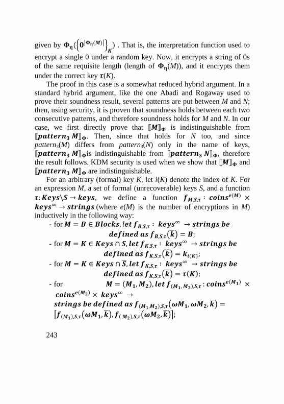
243

given by 𝚽𝛈({𝟎|𝚽𝛈(𝑴)|}

𝑲) . That is, the interpretation function used to

encrypt a single 0 under a random key. Now, it encrypts a string of 0s

of the same requisite length (length of 𝚽𝛈(M)), and it encrypts them

under the correct key 𝝉(K).

The proof in this case is a somewhat reduced hybrid argument. In a

standard hybrid argument, like the one Abadi and Rogaway used to

prove their soundness result, several patterns are put between M and N;

then, using security, it is proven that soundness holds between each two

consecutive patterns, and therefore soundness holds for M and N. In our

case, we first directly prove that ⟦𝑴⟧𝚽 is indistinguishable from

⟦𝒑𝒂𝒕𝒕𝒆𝒓𝒏𝟑 𝑴⟧𝚽. Then, since that holds for N too, and since

pattern3(M) differs from pattern3(N) only in the name of keys,

⟦𝒑𝒂𝒕𝒕𝒆𝒓𝒏𝟑 𝑴⟧𝚽is indistinguishable from ⟦𝒑𝒂𝒕𝒕𝒆𝒓𝒏𝟑 𝑵⟧𝚽, therefore

the result follows. KDM security is used when we show that ⟦𝑴⟧𝚽 and

⟦𝒑𝒂𝒕𝒕𝒆𝒓𝒏𝟑 𝑴⟧𝚽 are indistinguishable.

For an arbitrary (formal) key K, let i(K) denote the index of K. For

an expression M, a set of formal (unrecoverable) keys S, and a function

𝝉:𝑲𝒆𝒚𝒔\𝑺 → 𝒌𝒆𝒚𝒔, we define a function 𝒇𝑴,𝑺,𝝉 ∶ 𝒄𝒐𝒊𝒏𝒔𝒆(𝑴) ×

𝒌𝒆𝒚𝒔∞ → 𝒔𝒕𝒓𝒊𝒏𝒈𝒔 (where e(M) is the number of encryptions in M)

inductively in the following way:

- for 𝑴 = 𝑩 ∈ 𝑩𝒍𝒐𝒄𝒌𝒔, 𝑙𝒆𝒕 𝒇𝑩,𝑺,𝝉 ∶ 𝒌𝒆𝒚𝒔∞ → 𝒔𝒕𝒓𝒊𝒏𝒈𝒔 𝒃𝒆

𝒅𝒆𝒇𝒊𝒏𝒆𝒅 𝒂𝒔 𝒇𝑩,𝑺,𝝉(�̅�) = 𝑩;

- for 𝑴 = 𝑲 ∈ 𝑲𝒆𝒚𝒔 ∩ 𝑺, 𝒍𝒆𝒕 𝒇𝑲,𝑺,𝝉 ∶ 𝒌𝒆𝒚𝒔∞ → 𝒔𝒕𝒓𝒊𝒏𝒈𝒔 𝒃𝒆

𝒅𝒆𝒇𝒊𝒏𝒆𝒅 𝒂𝒔 𝒇𝑲,𝑺,𝝉(�̅�) = 𝒌𝒊(𝑲);

- for 𝑴 = 𝑲 ∈ 𝑲𝒆𝒚𝒔 ∩ �̅�, 𝒍𝒆𝒕 𝒇𝑲,𝑺,𝝉 ∶ 𝒌𝒆𝒚𝒔∞ → 𝒔𝒕𝒓𝒊𝒏𝒈𝒔 𝒃𝒆

𝒅𝒆𝒇𝒊𝒏𝒆𝒅 𝒂𝒔 𝒇𝑲,𝑺,𝝉(�̅�) = 𝝉(𝑲);

- for 𝑴 = (𝑴𝟏,𝑴𝟐), 𝒍𝒆𝒕 𝒇(𝑴𝟏, 𝑴𝟐),𝑺,𝝉 : 𝒄𝒐𝒊𝒏𝒔𝒆(𝑴𝟏) ×

𝒄𝒐𝒊𝒏𝒔𝒆(𝑴𝟐) × 𝒌𝒆𝒚𝒔∞ →𝒔𝒕𝒓𝒊𝒏𝒈𝒔 𝒃𝒆 𝒅𝒆𝒇𝒊𝒏𝒆𝒅 𝒂𝒔 𝒇(𝑴𝟏,𝑴𝟐),𝑺,𝝉(𝝎𝑴𝟏, 𝝎𝑴𝟐, �̅�) =

[𝒇(𝑴𝟏),𝑺,𝝉(𝝎𝑴𝟏, �̅�), 𝒇( 𝑴𝟐),𝑺,𝝉(𝝎𝑴𝟐, �̅�)];

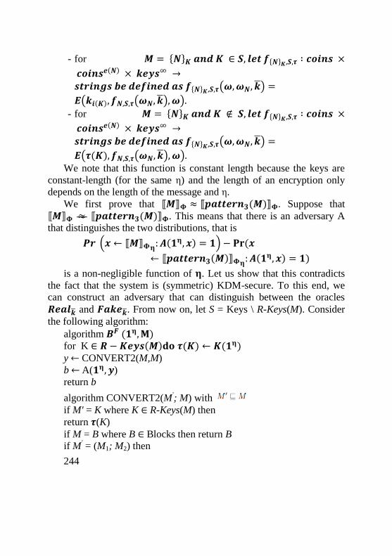
244

- for 𝑴 = {𝑵}𝑲 𝒂𝒏𝒅 𝑲 ∈ 𝑺, 𝒍𝒆𝒕 𝒇{𝑵}𝑲,𝑺,𝝉 ∶ 𝒄𝒐𝒊𝒏𝒔 ×

𝒄𝒐𝒊𝒏𝒔𝒆(𝑵) × 𝒌𝒆𝒚𝒔∞ →𝒔𝒕𝒓𝒊𝒏𝒈𝒔 𝒃𝒆 𝒅𝒆𝒇𝒊𝒏𝒆𝒅 𝒂𝒔 𝒇{𝑵}𝑲,𝑺,𝝉(𝝎,𝝎𝑵, �̅�) =

𝑬(𝒌𝒊(𝑲), 𝒇𝑵,𝑺,𝝉(𝝎𝑵, �̅�), 𝝎).

- for 𝑴 = {𝑵}𝑲 𝒂𝒏𝒅 𝑲 ∉ 𝑺, 𝒍𝒆𝒕 𝒇{𝑵}𝑲,𝑺,𝝉 ∶ 𝒄𝒐𝒊𝒏𝒔 ×

𝒄𝒐𝒊𝒏𝒔𝒆(𝑵) × 𝒌𝒆𝒚𝒔∞ →𝒔𝒕𝒓𝒊𝒏𝒈𝒔 𝒃𝒆 𝒅𝒆𝒇𝒊𝒏𝒆𝒅 𝒂𝒔 𝒇{𝑵}𝑲,𝑺,𝝉(𝝎,𝝎𝑵, �̅�) =

𝑬(𝝉(𝑲), 𝒇𝑵,𝑺,𝝉(𝝎𝑵, �̅�), 𝝎). We note that this function is constant length because the keys are

constant-length (for the same η) and the length of an encryption only

depends on the length of the message and η.

We first prove that ⟦𝑴⟧𝚽 ≈ ⟦𝒑𝒂𝒕𝒕𝒆𝒓𝒏𝟑(𝑴)⟧𝚽. Suppose that

⟦𝑴⟧𝚽 ≈ ⟦𝒑𝒂𝒕𝒕𝒆𝒓𝒏𝟑(𝑴)⟧𝚽. This means that there is an adversary A

that distinguishes the two distributions, that is

𝑷𝒓 (𝒙 ← ⟦𝑴⟧𝚽𝛈: 𝑨(𝟏𝛈, 𝒙) = 𝟏) − 𝐏𝐫 (𝒙

← ⟦𝒑𝒂𝒕𝒕𝒆𝒓𝒏𝟑(𝑴)⟧𝚽𝛈: 𝑨(𝟏𝛈, 𝒙) = 𝟏)

is a non-negligible function of 𝛈. Let us show that this contradicts

the fact that the system is (symmetric) KDM-secure. To this end, we

can construct an adversary that can distinguish between the oracles

𝑹𝒆𝒂𝒍�̅� and 𝑭𝒂𝒌𝒆�̅�. From now on, let S = Keys \ R-Keys(M). Consider

the following algorithm:

algorithm 𝑩𝑭 (𝟏𝛈,𝐌) for K ∈ 𝑹 −𝑲𝒆𝒚𝒔(𝑴)𝐝𝐨 𝝉(𝑲) ← 𝑲(𝟏𝛈) y ← CONVERT2(M,M)

b ← A(𝟏𝛈, 𝒚)

return b

algorithm CONVERT2(M'; M) with

if M' = K where K ∈ R-Keys(M) then

return 𝝉(K)

if M = B where B ∈ Blocks then return B

if M' = (M1; M2) then

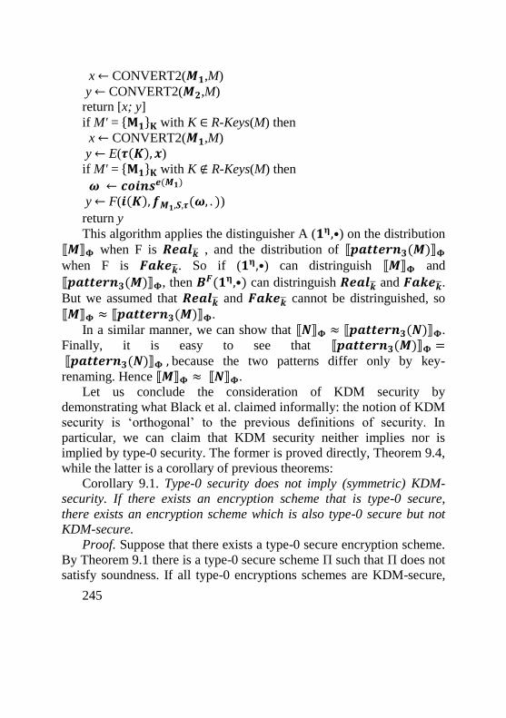
245

x ← CONVERT2(𝑴𝟏,M)

y ← CONVERT2(𝑴𝟐,M)

return [x; y]

if M' = {𝐌𝟏}𝐊 with K ∈ R-Keys(M) then

x ← CONVERT2(𝑴𝟏,M)

y ← E(𝝉(𝑲), 𝒙)

if M' = {𝐌𝟏}𝐊 with K ∉ R-Keys(M) then

𝝎 ← 𝒄𝒐𝒊𝒏𝒔𝒆(𝑴𝟏) y ← F(𝒊(𝑲), 𝒇𝑴𝟏,𝑺,𝝉(𝝎, . ))

return y

This algorithm applies the distinguisher A (𝟏𝛈,•) on the distribution

⟦𝑴⟧𝚽 when F is 𝑹𝒆𝒂𝒍�̅� , and the distribution of ⟦𝒑𝒂𝒕𝒕𝒆𝒓𝒏𝟑(𝑴)⟧𝚽

when F is 𝑭𝒂𝒌𝒆�̅�. So if (𝟏𝛈,•) can distringuish ⟦𝑴⟧𝚽 and

⟦𝒑𝒂𝒕𝒕𝒆𝒓𝒏𝟑(𝑴)⟧𝚽, then 𝑩𝑭(𝟏𝛈,•) can distringuish 𝑹𝒆𝒂𝒍�̅� and 𝑭𝒂𝒌𝒆�̅�.

But we assumed that 𝑹𝒆𝒂𝒍�̅� and 𝑭𝒂𝒌𝒆�̅� cannot be distringuished, so

⟦𝑴⟧𝚽 ≈ ⟦𝒑𝒂𝒕𝒕𝒆𝒓𝒏𝟑(𝑴)⟧𝚽.

In a similar manner, we can show that ⟦𝑵⟧𝚽 ≈ ⟦𝒑𝒂𝒕𝒕𝒆𝒓𝒏𝟑(𝑵)⟧𝚽.

Finally, it is easy to see that ⟦𝒑𝒂𝒕𝒕𝒆𝒓𝒏𝟑(𝑴)⟧𝚽 = ⟦𝒑𝒂𝒕𝒕𝒆𝒓𝒏𝟑(𝑵)⟧𝚽 , because the two patterns differ only by key-

renaming. Hence ⟦𝑴⟧𝚽 ≈ ⟦𝑵⟧𝚽.

Let us conclude the consideration of KDM security by

demonstrating what Black et al. claimed informally: the notion of KDM

security is ‘orthogonal’ to the previous definitions of security. In

particular, we can claim that KDM security neither implies nor is

implied by type-0 security. The former is proved directly, Theorem 9.4,

while the latter is a corollary of previous theorems:

Corollary 9.1. Type-0 security does not imply (symmetric) KDM-

security. If there exists an encryption scheme that is type-0 secure,

there exists an encryption scheme which is also type-0 secure but not

KDM-secure.

Proof. Suppose that there exists a type-0 secure encryption scheme.

By Theorem 9.1 there is a type-0 secure scheme Π such that Π does not

satisfy soundness. If all type-0 encryptions schemes are KDM-secure,

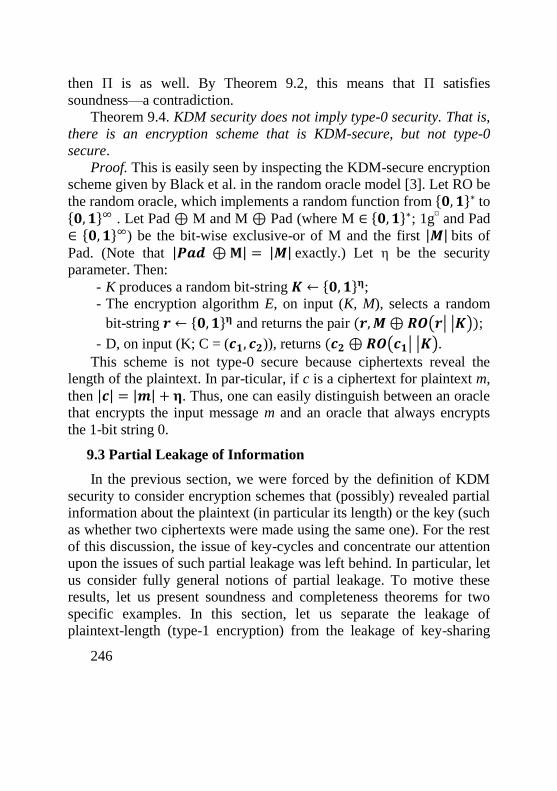
246

then Π is as well. By Theorem 9.2, this means that Π satisfies

soundness—a contradiction.

Theorem 9.4. KDM security does not imply type-0 security. That is,

there is an encryption scheme that is KDM-secure, but not type-0

secure.

Proof. This is easily seen by inspecting the KDM-secure encryption

scheme given by Black et al. in the random oracle model [3]. Let RO be

the random oracle, which implements a random function from {𝟎, 𝟏}∗ to {𝟎, 𝟏}∞ . Let Pad ⊕ M and M ⊕ Pad (where M ∈ {𝟎, 𝟏}∗; 1g

¤ and Pad

∈ {𝟎, 𝟏}∞) be the bit-wise exclusive-or of M and the first |𝑴| bits of

Pad. (Note that |𝑷𝒂𝒅 ⊕𝐌| = |𝑴| exactly.) Let η be the security

parameter. Then:

- K produces a random bit-string 𝑲 ← {𝟎, 𝟏}𝛈;

- The encryption algorithm E, on input (K, M), selects a random

bit-string 𝒓 ← {𝟎, 𝟏}𝛈 and returns the pair (𝒓,𝑴⊕𝑹𝑶(𝒓| |𝑲));

- D, on input (K; C = (𝒄𝟏, 𝒄𝟐)), returns (𝒄𝟐⊕𝑹𝑶(𝒄𝟏| |𝑲). This scheme is not type-0 secure because ciphertexts reveal the

length of the plaintext. In par-ticular, if c is a ciphertext for plaintext m,

then |𝒄| = |𝒎| + 𝛈. Thus, one can easily distinguish between an oracle

that encrypts the input message m and an oracle that always encrypts

the 1-bit string 0.

9.3 Partial Leakage of Information

In the previous section, we were forced by the definition of KDM

security to consider encryption schemes that (possibly) revealed partial

information about the plaintext (in particular its length) or the key (such

as whether two ciphertexts were made using the same one). For the rest

of this discussion, the issue of key-cycles and concentrate our attention

upon the issues of such partial leakage was left behind. In particular, let

us consider fully general notions of partial leakage. To motive these

results, let us present soundness and completeness theorems for two

specific examples. In this section, let us separate the leakage of

plaintext-length (type-1 encryption) from the leakage of key-sharing

247

(type-2 encryption) and consider each separately. In particular, let us

show in this section that soundness can survive such leakage in the

computational model if the formal model is appropriately weakened to

match.

Soundness and Completeness for Type-1 Schemes

Let us consider the case of ‘type-1’ encryption schemes: encryption

schemes which may reveal plaintext-length, but which conceals

whether or not two ciphertexts were created using the same key. (In the

terminology of Abadi and Rogaway, type-1 encryption is message-

concealing and which-key concealing, but may be length-revealing.)

An equivalent way to express this security definition is that no

adversary should be able to tell whether two ciphertexts were created

using the same key or different (independent) keys, even if the

adversary is allowed to choose the plaintexts, so long as those

plaintexts have the same length:

Definition 9.20 (Type-1 Security). Let ∏ = (K; E; D) be a

symmetric encryption scheme. We say that the encryption-scheme is

type-1 secure if no PPT adversary A can distinguish the pair of oracles

(E(k,•), E(k', •))) and (𝑬(𝒌, 𝟎|•|), 𝑬(𝒌, 𝟎|•|)) as k and k' are

independently generated, that is, for all PPT adversaries A:

𝑷𝒓[𝒌, 𝒌′ ← 𝑲(𝟏𝛈): 𝑨𝑬(𝒌,•),𝑬(𝒌′,•)(𝟏𝛈) = 𝟏]

− 𝑷𝒓 [𝒌 ← 𝑲(𝟏𝛈): 𝑨𝑬(𝒌,𝟎|•|),𝑬(𝒌,𝟎|•|)(𝟏𝛈) ≤ 𝒏𝒆𝒈 (𝛈)]

Type-1 security does not provide soundness for the logic of

Definition 9.1. For example, one can see immediately that {𝟎}𝑲𝟏 ≅

{𝟎𝟎}𝑲𝟏, but ⟦{𝟎}𝑲𝟏⟧𝚽≈ ⟦{𝟎𝟎}𝑲𝟏⟧𝚽

if the encryption scheme reveals

the length of the plaintext.

To show soundness or completeness, patterns must reflect those

aspects of an expression that an adversary can and cannot see. The idea

is similar to the one in Definition 9.16, but now “boxes” are indexed

with the only properties leaked by type-1 encryption: the formal length

248

of the plaintext. (Note, however, that the notions of visible-

subexpressions, recoverable keys and formal length remain unchanged.)

Definition 9.21 (Pattern (Type-1)). We define the set of patterns,

Pat, by the grammar:

Pat ::= Keys | Blocks | (Pat; Pat) | {𝑷𝒂𝒕}𝑲𝒆𝒚𝒔 | 𝒍(𝐄𝐱𝐩)

The type-1 pattern of an expression M, denoted by pattern1(M), is

derived from M by replacing each term {𝑴′}𝑲 ∈ 𝐯𝐢𝐬 (𝐌) (𝐰𝐡𝐞𝐫𝐞 𝐊 ∉𝐑 − 𝐊𝐞𝐲𝐬(𝐌)) by 𝒍(𝐌′).

We say that two expressions M and N are type-1 equivalent, and

denote it by 𝑴 ≅𝟏 𝑵, if there exists a key-renaming function 𝝈

pattern1(M) =𝟏 pattern1(N𝝈) where =𝟏 is defined in the following way:

- if P ∈ Blocks ∪ Keys, then P =1 Q iff P and Q are identical;

- if P is of the form 𝒍(𝐌′), then P =1 Q iff Q is of the form

𝒍(𝐍′),, and l(M') = l(N') in the sense of Definition 9.15;

- if P is of the form (P1; P2), then P =1 Q iff Q is of the form (Q1;

Q2) where P1 =1 Q1 and P2 =1 Q2;

- if P is of the form {𝑷′}𝑲 , then P =1 Q iff Q is of the form {𝑸′}𝑲

where P ' =1 Q'.

Again, the symbol 𝒍(𝐌′) in a pattern reveals that some plaintext is

encrypted and its length is l(M').

Example 9.2. Let N be the expression

(({𝟎}𝑲𝟖 , {𝟏𝟎𝟎}𝑲𝟏), ((𝑲𝟕, {({𝟏𝟎𝟏}𝑲𝟗 , {𝑲𝟖}𝑲𝟓)}𝑲𝟓, {𝑲𝟓}𝑲𝟕)).

We have that R-Keys(N) = {𝑲𝟓, 𝑲𝟕, 𝑲𝟖}, and so, in this case,

pattern1(N) is

(({𝟎}𝑲𝟖 , 𝒍(𝟏𝟎𝟎) ), ((𝑲𝟕, {( 𝒍(𝟏𝟎𝟏), {𝑲𝟖}𝑲𝟓)}𝑲𝟓) , {𝑲𝟓}𝑲𝟕)).

Defining M as in Example 9.1, pattern1(M) is

(({𝟎}𝑲𝟔 , 𝒍({𝑲𝟕}𝑲𝟏)) , ((𝑲𝟐, {( 𝒍(𝟎𝟎𝟏), {𝑲𝟔}𝑲𝟓)}𝑲𝟓

) , {𝑲𝟓}𝑲𝟐)).

Now, if we replace 𝑲𝟔 → 𝑲𝟖, 𝑲2 → 𝑲𝟕 𝐚𝐧𝐝 𝑲𝟓 → 𝑲𝟓 in M, we

have that 𝑴 ≅𝟏 𝑵 𝐢𝐟𝐟 𝒍(𝟏𝟎𝟎) = 𝒍({𝑲𝟕}𝑲𝟏).

249

With these definitions, the following soundness and completeness

theorems can be proved.

Theorem 9.5 (Type-1 Soundness). Let ∏ be a type-1 secure

encryption scheme such that for all k ∈ keys; m ∈ plaintexts and w; w'

∈ coins we have |𝑬(𝒌,𝒎,𝒘)| = |𝑬(𝒌,𝒎,𝒘′)| . Then, if the length-

function satisfies only the equalities defined in Definition 2.15, then for

any M and N expressions such that B-Keys(M) and B-Keys(N) are not

cyclic in M and N respectively,

𝐌 ≅𝟏 𝐍 implies ⟦𝐌⟧𝚽 ≈ ⟦𝐍⟧𝚽.

Otherwise, for arbitrary length-function l (that is, one satisfying

possible more equations), if for all pairs of expressions M and N, l (M)

= l (N) implies that the binary length of ⟦𝑴⟧𝜱𝜼 is the same as the

binary length of ⟦𝑵⟧𝜱𝜼 for each security parameter ´, then for any M

and N expressions,

𝑴 ≅𝟏 𝑵 implies ⟦𝑴⟧𝚽 ≈ ⟦𝑵⟧𝚽.

In addition to soundness, also let us demonstrate the completeness.

If soundness shows that formal in-distinguishability implies

computational indistinguishability, completeness shows the converse.

Rephrased, completeness implies that formal distinguishability (as

opposed to indistinguishability) implies computational

distinguishability. For this to be true, the interpretation function must

en-force a handful of ‘atomic’ distinguishability properties:

Theorem 9.6 (Type-1 Completeness). Let ∏ be a type-1 secure

encryption scheme such that |𝑬(𝒌,𝒎,𝒘)| = |𝑬(𝒌,𝒎,𝒘′)| for all k ∈

keys; m ∈ plaintexts and w; w' ∈ coins. We have:

⟦𝑴⟧𝚽 ≈ ⟦𝑵⟧𝚽 implies 𝑴 ≅𝟏 𝑵

for all M and N pairs of expressions if and only if the following

conditions hold: for any

K; K'; K'' ∈ Keys, B ∈ Blocks, M; M'; N ∈ Exp,

(i) no pair of ⟦𝑲⟧𝚽, ⟦𝑩⟧𝚽, ⟦𝑲(𝑴,𝑵)⟧𝚽, ⟦{𝑴′}𝑲′⟧𝚽 are equivalent

with respect to ≈,

(ii) if ⟦(𝑲, {𝑴}𝑲)⟧𝚽 ≈ ⟦(𝑲′′, {𝑴′}𝑲′)⟧𝚽 , then K' = K'', and

(iii) if ⟦{𝑴}𝑲⟧𝚽 ≈ ⟦{𝑴′}𝑲′⟧𝚽 then l(M) = l (M').

250

Some aspects of this theorem merit further discussion. First, note

that the theorem does not mention key-cycles. Secondly, note that

Condition (i) requires that different types of ob-jects, blocks, keys, pairs

and encryption terms should be distinguishable to achieve complete-

ness; this can be ensured by tagging each object with its type, as

suggested in [2]. Thirdly, Condition (ii) (which we call weak confusion-

freeness) is equivalent to the property of weak key-authenticity

introduced by Horvitz and Gligor [6] in the case of type-0 schemes.

This property essentially means that decrypting with the wrong key

should be detectable in a proba-bilistic sense. Finally, condition (iii)

requires that encryption of messages with different length should be

detectable. Definition 2.20 allows that encryptions of messages of

different length may be detected but does not enforce it. That suffices

for soundness, but completeness requires that it should be detectable

when ciphertexts contain messages of different lengths. A purely

computational condition that implies condition (iii) is the notion of

strictly length revealing:

Definition 9.22 (Strictly Length Revealing Scheme). Let ∏ = (K; E;

D) be a symmetric en-cryption scheme. We say that the encryption-

scheme is strictly length revealing if it is type-1 secure but there exists

a PPT adversary A such that the following function is a non-negligible

function of η:

𝑷𝒓[𝒌 ← 𝑲(𝟏𝛈) ∶ 𝑨𝑬(𝒌,•)(𝟏𝛈) = 𝟏]

− 𝑷𝒓 [𝒌 ← 𝑲(𝟏𝛈) ∶ 𝑨𝑬(𝒌,𝟎≠|•|)(𝟏𝛈) = 𝟏]

We use 𝟎≠|•| to denote 0n, where 𝒏 ≠ |•|.

Soundness and Completeness for Type-2 Schemes

Having considered the leakage of plaintext-length in the previous

section, let us turn to the other to the kinds of leakage seen in KDM-

security: whether or not two ciphertext share a key. However, we can

now assume that the plaintext conceals the plaintext-length. (‘Type-2’

in the terminology of Abadi and Rogaway, as well as message-

concealing, length-concealing, and which-key reveal-ing.) For this type

251

of encryption, no adversary should be able to tell whether a ciphertext

contains a (possibly long) plaintext or the single-bit plaintext 0:

Definition 9.23 (Type-2 Security). Let ∏ = (K; E; D) be a

symmetric encryption scheme. We say that the encryption-scheme is

type-2 secure if no PPT adversary A can distinguish the oracles E(k; •)

and E(k; 0) as k is randomly generated, that is, for all PPT adversaries

A:

𝑷𝒓[𝒌 ← 𝑲(𝟏𝛈) ∶ 𝑨𝑬(𝒌,•)(𝟏𝛈) = 𝟏]

− 𝑷𝒓[𝒌 ← 𝑲(𝟏𝛈) ∶ 𝑨𝑬(𝒌,𝟎)(𝟏𝛈) = 𝟏] ≤ 𝒏𝒆𝒈(𝛈) Again, patterns must be re-defined to reflect all the information

about an expression which may be available to the adversary, but only

that information:

Definition 9.24 (Pattern (Type-2)). We define the set of patterns,

Pat, by the grammar:

Pat ::= Keys | Blocks | (Pat; Pat) | {𝑷𝒂𝒕}𝑲𝒆𝒚𝒔 | 𝑲𝒆𝒚𝒔

The type-2 pattern of expression M, denoted be pattern2(M), is

derived from M by replacing each term {𝑴′}𝑲 ∈ vis (M) (where K ∉ R-

Keys(M)) by 𝑲.

We say that two expression M and N are type-2 equivalent, and

denote it by 𝑴 ≅𝟐 𝑵, if there exist a key-renaming function σ such that

𝒑𝒂𝒕𝒕𝒆𝒓𝒏𝟐(𝑴) =𝟐 𝒑𝒂𝒕𝒕𝒆𝒓𝒏𝟐(𝑵𝝈) where =𝟐 is defined in the

following way:𝟐

- if P ∈ Blocks ∪ Keys, then P =2 Q iff P and Q are identical;

- if P is of the form 𝑲 , then P =2 Q iff Q is also of the form 𝑲 ;

- if P is of the form (P1; P2), then P =2 Q iff Q is of the form (Q1;

Q2) where P1 =2 Q1 and P2 =2 Q2.;

- if P is of the form {𝑷′}𝑲, then P =2 Q iff Q is of the form {𝑸′}𝑲,

where P ' =2 Q'.

Example 9.3. Let N be the same expression as in Example 9.2,

(({𝟎}𝑲𝟖 , {𝟏𝟎𝟎}𝑲𝟏), ((𝑲𝟕{({𝟏𝟎𝟏}𝑲𝟗 , {𝑲𝟖}𝑲𝟓)}𝑲𝟓) , {𝑲𝟓}𝑲𝟕)).

252

We have that R-Keys(N) = {𝑲𝟓, 𝑲𝟕, 𝑲𝟖} , and so, in this case,

pattern2(N) is

(({𝟎}𝑲𝟖 , 𝑲𝟏 ), ((𝑲𝟕{( 𝑲𝟗 , {𝑲𝟖}𝑲𝟓)}𝑲𝟓) , {𝑲𝟓}𝑲𝟕)).

Defining M as in Example 9.1, pattern2(M) is

(({𝟎}𝑲𝟔 , 𝑲𝟒 ), ((𝑲𝟐{( 𝑲𝟑 , {𝑲𝟔}𝑲𝟓)}𝑲𝟓) , {𝑲𝟓}𝑲𝟐)).

Now, if we replace 𝑲𝟔 → 𝑲𝟖, 𝑲𝟒 → 𝑲𝟏, 𝑲𝟐 → 𝑲𝟕, 𝑲𝟑 → 𝑲𝟗, and

𝑲𝟓 → 𝑲𝟓, in M , we have that 𝑴 ≅𝟐 𝑵.

With these definitions, the following soundness and completeness

theorems can be proved.

Theorem 9.8 (Type-2 Completeness). Let ∏ be a type-2 secure

encryption scheme. We have

⟦𝑴⟧𝚽 ≈ ⟦𝑵⟧𝚽 𝒊𝒎𝒑𝒍𝒊𝒆𝒔 𝑴 ≅𝟐 𝑵 that, for any pairs of expressions M and N if and only if the

following conditions hold: for any

K; K'; K

'' ∈ Keys, B ∈ Blocks, M; M

'; N; N

' ∈ Exp,

(i) no pair of ⟦𝑲⟧𝚽, ⟦𝑩⟧𝚽, ⟦(𝑴,𝑵)⟧𝚽, ⟦{𝑴′}𝑲′⟧𝚽 are equivalent

with respect to≈;

(ii) if ⟦(𝑲, {𝑴}𝑲)⟧𝚽 ≈ ⟦(𝑲′′, {𝑴′}𝑲′)⟧𝚽, then K' = K'';

(iii) if ⟦({𝑴}𝑲, {𝑴′}𝑲⟧𝚽 ≈ ⟦({𝑵}𝑲′, {𝑵′}𝑲′′⟧𝚽 then K' = K''.

The conditions of the completeness theorem are similar to the ones

for the type-1 case ex-cept for condition (iii). This condition requires

that encryption with different keys should be detectable. Definition 9.23

allows that encrypting with different keys may be detectable, but it does

not require it. That suffices for soundness, but such detection is

required for completeness. It is easily shown that condition (iii) is

implied by the purely computational definition of a strictly key

revealing encryption scheme:

Definition 9.25 (Strictly Key Revealing Scheme). Let ∏ = (K; E; D) be a symmetric encryp-tion scheme. We say that the encryption-

scheme is strictly key revealing if it is type-2 secure but there exists a

253

PPT adversary A such that the following function is a non-negligible

function of η:

𝑷𝒓[𝒌, 𝒌′ ← 𝑲(𝟏𝛈) ∶ 𝑨𝑬(𝒌,•),𝑬(𝒌′,•)(𝟏𝛈) = 𝟏]

− 𝑷𝒓[𝒌 ← 𝑲(𝟏𝛈) ∶ 𝑨𝑬(𝒌,•),𝑬(𝒌,•)(𝟏𝛈) = 𝟏] 9.3.3 Soundness and Completeness for Type-3 Schemes

Type-3 encryption schemes (Definition 9.14, also called message-

concealing, which-key reveal-ing and length-revealing in the

terminology of Abadi and Rogaway) can be thought of as leaking the

information leaked by both type-1 and type-2 schemes. Both soundness

and completeness results follow using the notion of patterns from

Definition 9.16. As with type-1 and type-2 en-cryption, completeness

requires that it is possible to distinguish ciphertexts that were encrypted

with different keys, and to distinguish ciphertexts for which the

plaintexts have different lengths. That is, the encryption scheme must

be both strictly key revealing and strictly length revealing (Definitions

2.25 and 2.22 respectively).

9.4 Information-Theoretic Interpretations: Soundness and

Completeness for One-Time Pad

Besides the computational definition, there are other possible

important notions of ‘indistin-guishability.’ For example, we could say

that two distributions are ‘indistinguishable’ if and only if they are

identical. Such a notion would lead to new (but analogous) notions of

soundness and completeness, and we can explore these new notions

using (as a specific encryption scheme) the One-Time Pad (OTP).

Let strings ≔ {𝟎, 𝟏}∗with the following pairing function: For any

two strings x; y ∈ strings we can define the pairing of x and y as

[𝒙, 𝒚] ≔ ⟨𝒙, 𝒚, 𝟎, 𝟏|𝒚|⟩ 𝒘𝒉𝒆𝒓𝒆 ⟨ , , … , ⟩i denotes the concatenation of the

strings separated by the commas, 1m stands for m many 1’s, and for any

x 𝒙 ∈ {𝟎, 𝟏}∗, |𝒙|denotes the length of the string. The number of 1’s at

the end indicate how long the second string is in the pair, and the 0

separates the strings from the 1’s. Let blocks be those strings that end

254

with 001. The ending is just a tag, it shows that the meaning of the

string is a block.

Key-Generation. In case of the OTP, the length of the encrypting

key must match the length of the plaintext. Thus, we need a separate

key-generation for each length. That is, for each n > 3, Kn is a random

variable over some discrete probability field such that

its values are equally distributed over

𝒌𝒆𝒚𝒔𝒏 ≔ {𝒌 | 𝒌 ∈ 𝒔𝒕𝒓𝒊𝒏𝒈𝒔, |𝒌| = 𝒏, 𝒌 𝒆𝒏𝒅𝒔 𝒘𝒊𝒕𝒉 𝟎𝟏𝟎}. Let

𝒌𝒆𝒚𝒔 ∶=∪𝟒∞ 𝒌𝒆𝒚𝒔𝒏. For k ∈ keys, let core(k) denote the string that we

get from k by cutting the tag 010.

Encryption. Let the domain of the encryption function, DomE , be

those elements (k; x) ∈ keys × strings, for which |𝒌| = |𝒙| + 𝟑, and let

𝑬(𝒌, 𝒙) ≔ ⟨𝒄𝒐𝒓𝒆(𝒌)⊕ 𝐱, 𝟏𝟏𝟎⟩ . The tag 110 informs us that the string

is a ciphertext. Notice that this encryption is not probabilistic, hence

𝑬(𝒌, 𝒙) is not a random variable. Notice also, that the tag of the

plaintext is not dropped, that part is also encrypted.

Decryption. The decryption function 𝑫(𝒌, 𝒙) is defined

whenever |𝒌| = |𝒙|, and, naturally the value of 𝑫(𝒌, 𝒙) is the first

|𝒌| − 𝟑 𝒃𝒊𝒕𝒔 𝒐𝒇 𝒌 ⊕ 𝐱.

Indistinguishability. Let us now call two distributions

indistinguishable, if they are identical, and denote this relation by =d.

As in the case of type-3 encryption, lengths of the messages are

revealed. Therefore, we must again define the length of an expression.

Definition 9.26. We assume that some length function 𝒍 ∶ 𝑲𝒆𝒚𝒔 →{𝟒, 𝟓,… } is given on the keys symbols. The length of a block is defined

as 𝒍(𝑩) ≔ |𝑩| + 𝟑. We added 3 to match the length of the tag. We

define the length function on any expression in Exp by induction:

- 𝒍((𝑴,𝑵)) ≔ 𝒍(𝑴) + 𝟐𝒍(𝑵) + 𝟏,

- 𝒍({𝑴}𝑲) ≔ 𝒍(𝑴) + 𝟑, 𝒊𝒇 𝒍(𝑴) = 𝒍(𝑲) − 𝟑, 𝒂𝒏𝒅

- 𝒍({𝑴}𝑲) ≔ 𝟎, 𝑖𝒇 𝒍(𝑴) ≠ 𝒍(𝑲) − 𝟑. The valid expressions are defined as those expressions in which the

length of the encrypted subexpressions match the length of the

encrypting key, and, in which no key is used twice to en-crypt. (This

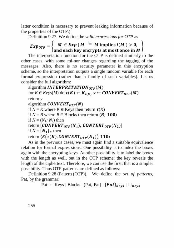
255

latter condition is necessary to prevent leaking information because of

the properties of the OTP.)

Definition 9.27. We define the valid expressions for OTP as

𝑬𝒙𝒑𝑶𝑻𝑷 = {𝑴 ∈ 𝑬𝒙𝒑 | 𝑴′ 𝑴 𝐢𝐦𝐩𝐥𝐢𝐞𝐬 𝒍(𝑴′) > 𝟎,

𝐚𝐧𝐝 𝐞𝐚𝐜𝐡 𝐤𝐞𝐲 𝐞𝐧𝐜𝐫𝐲𝐩𝐭𝐬 𝐚𝐭 𝐦𝐨𝐬𝐭 𝐨𝐧𝐜𝐞 𝐢𝐧 𝑴 }.

The interpretation function for the OTP is defined similarly to the

other cases, with some mi-nor changes regarding the tagging of the

messages. Also, there is no security parameter in this encryption

scheme, so the interpretation outputs a single random variable for each

formal ex-pression (rather than a family of such variables). Let us

consider the full algorithm:

algorithm 𝑰𝑵𝑻𝑬𝑹𝑷𝑹𝑬𝑻𝑨𝑻𝑰𝑶𝑵𝑶𝑻𝑷(𝑴) for K ∈ Keys(M) do 𝝉(𝑲) ← 𝑲𝒍(𝑲) 𝒚 ← 𝑪𝑶𝑵𝑽𝑬𝑹𝑻𝑶𝑻𝑷(𝑴)

return y

algorithm 𝑪𝑶𝑵𝑽𝑬𝑹𝑻𝑶𝑻𝑷(𝑵) if N = K where K ∈ Keys then return 𝝉(K)

if N = B where B ∈ Blocks then return ⟨𝑩; 𝟏𝟎𝟎⟩ if N = (N1; N2) then

return [𝑪𝑶𝑵𝑽𝑬𝑹𝑻𝑶𝑻𝑷(𝑵𝟏); 𝑪𝑶𝑵𝑽𝑬𝑹𝑻𝑶𝑻𝑷(𝑵𝟐)] if N = {𝑵𝟏}𝑲 then

return ⟨𝑬(𝝉(𝑲), 𝑪𝑶𝑵𝑽𝑬𝑹𝑻𝑶𝑻𝑷(𝑵𝟏)), 𝟏𝟏𝟎⟩ As in the previous cases, we must again find a suitable equivalence

relation for formal expres-sions. One possibility is to index the boxes

again with the encrypting keys. Another possibility is to label the boxes

with the length as well, but in the OTP scheme, the key reveals the

length of the ciphertext. Therefore, we can use the first, that is a simpler

possibility. Thus OTP-patterns are defined as follows:

Definition 9.28 (Pattern (OTP)). We define the set of patterns,

Pat, by the grammar:

Pat ::= Keys | Blocks | (Pat; Pat) | {𝑷𝒂𝒕}𝑲𝒆𝒚𝒔 | 𝑲𝒆𝒚𝒔

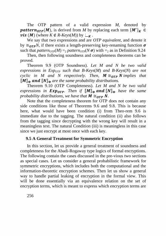
256

The OTP pattern of a valid expression M, denoted by

𝒑𝒂𝒕𝒕𝒆𝒓𝒏𝑶𝑻𝑷(𝑴), is derived from M by replacing each term {𝑴′}𝑲 ∈𝒗𝒊𝒔 (𝑴) (where K ∉ R-Keys(M)) by 𝑲 .

We say that two expressions and are OTP equivalent, and denote it

by ≅𝑶𝑻𝑷N, if there exists a length-preserving key-renaming function 𝝈

such that patternOTP(M) =2 patternOTP(N 𝝈) with =2 as in Definition 9.24

Then, then following soundness and completeness theorems can be

proved.

Theorem 9.9 (OTP Soundness). Let M and N be two valid

expressions in ExpOTP such that B-Keys(M) and B-Keys(N) are not

cyclic in M and N respectively. Then, 𝑴 ≅𝑶𝑻𝑷 𝑵 implies that ⟦𝑴⟧𝚽 𝒂𝒏𝒅 ⟦𝑵⟧𝚽 are the same probability distributions.

Theorem 9.10 (OTP Completeness). Let M and N be two valid

expressions in 𝑬𝒙𝒑𝑶𝑻𝑷. Then if ⟦𝑴⟧𝚽 𝒂𝒏𝒅 ⟦𝑵⟧𝚽 have the same

probability distributions, we have that 𝑴 ≅𝑶𝑻𝑷 𝑵. Note that the completeness theorem for OTP does not contain any

side conditions like those of Theorems 9.6 and 9.8. This is because

here, what would have been condition (i) from Theo-rem 9.6 is

immediate due to the tagging. The natural condition (ii) also follows

from the tagging since decrypting with the wrong key will result in a

meaningless text. The natural Condition (iii) is meaningless in this case

since we just encrypt at most once with each key.

9.5 A General Treatment for Symmetric Encryption

In this section, let us provide a general treatment of soundness and

completeness for the Abadi-Rogaway type logics of formal encryptions.

The following contain the cases discussed in the pre-vious two sections

as special cases. Let us consider a general probabilistic framework for

symmetric encryptions, which includes both the computational and the

information-theoretic encryption schemes. Then let us show a general

way to handle partial leaking of encryption in the formal view. This

will be done essentially via an equivalence relation on the set of

encryption terms, which is meant to express which encryption terms are

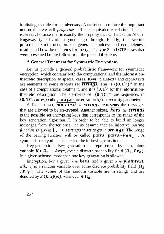
257

in-distinguishable for an adversary. Also let us introduce the important

notion that we call properness of this equivalence relation. This is

essential, because this is exactly the property that will make an Abadi-

Rogaway type hybrid argument go through. Finally, this section

presents the interpretation, the general soundness and completeness

results and how the theorems for the type-1, type-2 and OTP cases that

were presented before follow from the general theorems.

A General Treatment for Symmetric Encryptions

Let us provide a general probabilistic framework for symmetric

encryption, which contains both the computational and the information-

theoretic description as special cases. Keys, plaintexts and ciphertexts

are elements of some discrete set 𝒔𝒕𝒓𝒊𝒏𝒈𝒔̅̅ ̅̅ ̅̅ ̅̅ ̅̅ ̅. This is ({𝟎, 𝟏}∗)∞ in the

case of a computational treatment, and it is {𝟎, 𝟏}∗ for the information-

theoretic description. The ele-ments of ({𝟎, 𝟏}∗)∞ are sequences in {𝟎, 𝟏}∗, corresponding to a parameterisation by the security parameter.

A fixed subset, 𝒑𝒍𝒂𝒊𝒏𝒕𝒆𝒙𝒕̅̅ ̅̅ ̅̅ ̅̅ ̅̅ ̅̅ ̅̅ ⊆ 𝒔𝒕𝒓𝒊𝒏𝒈𝒔̅̅ ̅̅ ̅̅ ̅̅ ̅̅ ̅ represents the messages

that are allowed to be en-crypted. Another subset, 𝒌𝒆𝒚𝒔 ̅̅ ̅̅ ̅̅ ̅̅ ⊆ 𝒔𝒕𝒓𝒊𝒏𝒈𝒔̅̅ ̅̅ ̅̅ ̅̅ ̅̅ ̅ is the possible set encrypting keys that corresponds to the range of the

key generation algorithm K. In order to be able to build up longer

messages from shorter ones, let us assume that an injective pairing

function is given: [. , . ] ∶ 𝒔𝒕𝒓𝒊𝒏𝒈𝒔̅̅ ̅̅ ̅̅ ̅̅ ̅̅ ̅ × 𝒔𝒕𝒓𝒊𝒏𝒈𝒔̅̅ ̅̅ ̅̅ ̅̅ ̅̅ ̅ → 𝒔𝒕𝒓𝒊𝒏𝒈𝒔̅̅ ̅̅ ̅̅ ̅̅ ̅̅ ̅. The range

of the pairing function will be called 𝒑𝒂𝒊𝒓𝒔̅̅ ̅̅ ̅̅ ̅̅ : 𝒑𝒂𝒊𝒓𝒔̅̅ ̅̅ ̅̅ ̅̅ :=𝑹𝒂𝒏[.,.] . A

symmetric encryption scheme has the following constituents:

Key-generation. Key-generation is represented by a random

variable 𝑲 ∶ 𝛀𝑲 → 𝒌𝒆𝒚𝒔̅̅ ̅̅ ̅̅ ̅, over a discrete probability field (𝛀𝑲, 𝑷𝒓𝑲). In a given scheme, more than one key-generation is allowed.

Encryption. For a given k ∈ 𝒌𝒆𝒚𝒔̅̅ ̅̅ ̅̅ ̅, and a given x ∈ 𝒑𝒍𝒂𝒊𝒏𝒕𝒆𝒙𝒕̅̅ ̅̅ ̅̅ ̅̅ ̅̅ ̅̅ ̅̅ ,

E(k; x) is a random variable over some discrete probability field (𝛀𝑬

; 𝑷𝒓𝑬 ). The values of this random variable are in strings and are

denoted by E (𝒌, 𝒙)(𝝎), whenever ∈ 𝛀𝑬 .

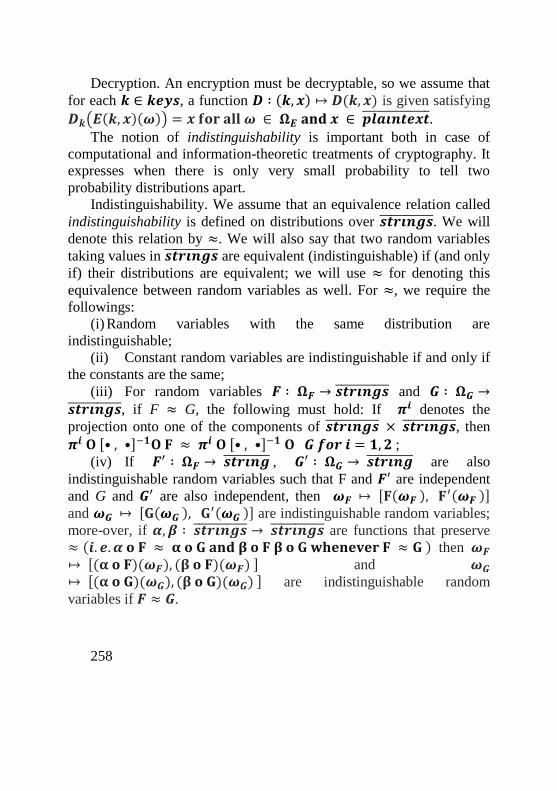
258

Decryption. An encryption must be decryptable, so we assume that

for each 𝒌 ∈ 𝒌𝒆𝒚𝒔, a function 𝑫 ∶ (𝒌, 𝒙) ↦ 𝑫(𝒌, 𝒙) is given satisfying

𝑫𝒌(𝑬(𝒌, 𝒙)(𝝎)) = 𝒙 𝐟𝐨𝐫 𝐚𝐥𝐥 𝝎 ∈ 𝛀𝑬 𝐚𝐧𝐝 𝒙 ∈ 𝒑𝒍𝒂𝒊𝒏𝒕𝒆𝒙𝒕̅̅ ̅̅ ̅̅ ̅̅ ̅̅ ̅̅ ̅̅ .

The notion of indistinguishability is important both in case of

computational and information-theoretic treatments of cryptography. It

expresses when there is only very small probability to tell two

probability distributions apart.

Indistinguishability. We assume that an equivalence relation called

indistinguishability is defined on distributions over 𝒔𝒕𝒓𝒊𝒏𝒈𝒔̅̅ ̅̅ ̅̅ ̅̅ ̅̅ ̅. We will

denote this relation by ≈. We will also say that two random variables

taking values in 𝒔𝒕𝒓𝒊𝒏𝒈𝒔̅̅ ̅̅ ̅̅ ̅̅ ̅̅ ̅ are equivalent (indistinguishable) if (and only

if) their distributions are equivalent; we will use ≈ for denoting this

equivalence between random variables as well. For ≈, we require the

followings:

(i) Random variables with the same distribution are

indistinguishable;

(ii) Constant random variables are indistinguishable if and only if

the constants are the same;

(iii) For random variables 𝑭 ∶ 𝛀𝑭 → 𝒔𝒕𝒓𝒊𝒏𝒈𝒔̅̅ ̅̅ ̅̅ ̅̅ ̅̅ ̅ and 𝑮 ∶ 𝛀𝑮 →𝒔𝒕𝒓𝒊𝒏𝒈𝒔̅̅ ̅̅ ̅̅ ̅̅ ̅̅ ̅, if F ≈ G, the following must hold: If 𝝅𝒊 denotes the

projection onto one of the components of 𝒔𝒕𝒓𝒊𝒏𝒈𝒔̅̅ ̅̅ ̅̅ ̅̅ ̅̅ ̅ × 𝒔𝒕𝒓𝒊𝒏𝒈𝒔̅̅ ̅̅ ̅̅ ̅̅ ̅̅ ̅, then

𝝅𝒊 𝚶 [• , •]−𝟏𝚶 𝐅 ≈ 𝝅𝒊 𝚶 [• , •]−𝟏 𝚶 𝑮 𝒇𝒐𝒓 𝒊 = 𝟏, 𝟐 ; (iv) If 𝑭′ ∶ 𝛀𝑭 → 𝒔𝒕𝒓𝒊𝒏𝒈̅̅ ̅̅ ̅̅ ̅̅ ̅̅ , 𝑮′ ∶ 𝛀𝑮 → 𝒔𝒕𝒓𝒊𝒏𝒈̅̅ ̅̅ ̅̅ ̅̅ ̅̅ are also

indistinguishable random variables such that F and 𝑭′ are independent

and G and 𝑮′ are also independent, then 𝝎𝑭 ↦ [𝐅(𝝎𝑭 ), 𝐅′(𝝎𝑭 )]

and 𝝎𝑮 ↦ [𝐆(𝝎𝑮 ), 𝐆′(𝝎𝑮 )] are indistinguishable random variables;

more-over, if 𝜶,𝜷 ∶ 𝒔𝒕𝒓𝒊𝒏𝒈𝒔̅̅ ̅̅ ̅̅ ̅̅ ̅̅ ̅ → 𝒔𝒕𝒓𝒊𝒏𝒈𝒔̅̅ ̅̅ ̅̅ ̅̅ ̅̅ ̅ are functions that preserve

≈ (𝒊. 𝒆. 𝜶 𝛐 𝐅 ≈ 𝛂 𝛐 𝐆 𝐚𝐧𝐝 𝛃 𝛐 𝐅 𝛃 𝛐 𝐆 𝐰𝐡𝐞𝐧𝐞𝐯𝐞𝐫 𝐅 ≈ 𝐆 ) then 𝝎𝑭

↦ [(𝛂 𝛐 𝐅)(𝝎𝑭), (𝛃 𝛐 𝐅)(𝝎𝑭) ] and 𝝎𝑮

↦ [(𝛂 𝛐 𝐆)(𝝎𝑮), (𝛃 𝛐 𝐆)(𝝎𝑮) ] are indistinguishable random

variables if 𝑭 ≈ 𝑮.

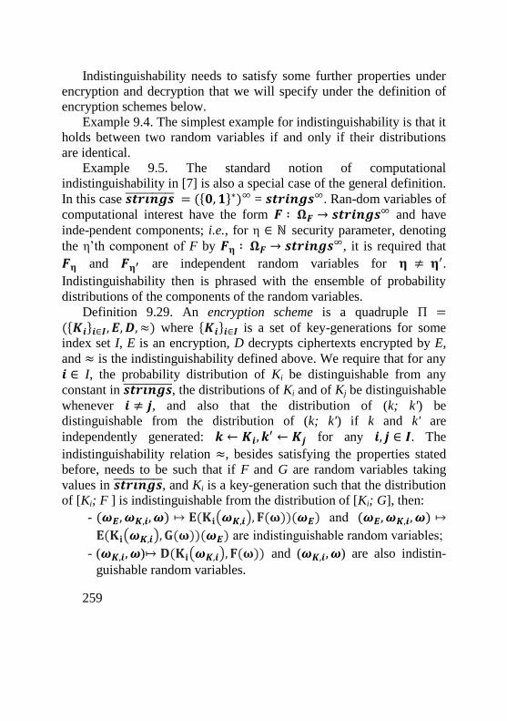
259

Indistinguishability needs to satisfy some further properties under

encryption and decryption that we will specify under the definition of

encryption schemes below.

Example 9.4. The simplest example for indistinguishability is that it

holds between two random variables if and only if their distributions

are identical.

Example 9.5. The standard notion of computational

indistinguishability in [7] is also a special case of the general definition.

In this case 𝒔𝒕𝒓𝒊𝒏𝒈𝒔̅̅ ̅̅ ̅̅ ̅̅ ̅̅ ̅ = ({𝟎, 𝟏}∗)∞ = 𝒔𝒕𝒓𝒊𝒏𝒈𝒔∞. Ran-dom variables of

computational interest have the form 𝑭 ∶ 𝛀𝑭 → 𝒔𝒕𝒓𝒊𝒏𝒈𝒔∞ and have

inde-pendent components; i.e., for η ∈ ℕ security parameter, denoting

the η’th component of F by 𝑭𝛈 ∶ 𝛀𝑭 → 𝒔𝒕𝒓𝒊𝒏𝒈𝒔∞, it is required that

𝑭𝛈 and 𝑭𝛈′ are independent random variables for 𝛈 ≠ 𝛈′.

Indistinguishability then is phrased with the ensemble of probability

distributions of the components of the random variables.

Definition 9.29. An encryption scheme is a quadruple Π =({𝑲𝒊}𝒊∈𝑰, 𝑬, 𝑫,≈) where {𝑲𝒊}𝒊∈𝑰 is a set of key-generations for some

index set I, E is an encryption, D decrypts ciphertexts encrypted by E,

and ≈ is the indistinguishability defined above. We require that for any

𝒊 ∈ I, the probability distribution of Ki be distinguishable from any

constant in 𝒔𝒕𝒓𝒊𝒏𝒈𝒔̅̅ ̅̅ ̅̅ ̅̅ ̅̅ ̅, the distributions of Ki and of Kj be distinguishable

whenever 𝒊 ≠ 𝒋, and also that the distribution of (k; k') be

distinguishable from the distribution of (k; k') if k and k' are

independently generated: 𝒌 ← 𝑲𝒊, 𝒌′ ← 𝑲𝒋 for any 𝒊, 𝒋 ∈ 𝑰. The

indistinguishability relation ≈, besides satisfying the properties stated

before, needs to be such that if F and G are random variables taking

values in 𝒔𝒕𝒓𝒊𝒏𝒈𝒔̅̅ ̅̅ ̅̅ ̅̅ ̅̅ ̅, and Ki is a key-generation such that the distribution

of [Ki; F ] is indistinguishable from the distribution of [Ki; G], then:

- (𝝎𝑬, 𝝎𝑲,𝒊, 𝝎) ↦ 𝐄(𝐊𝐢(𝝎𝑲,𝒊), 𝐅(𝛚))(𝝎𝑬) and (𝝎𝑬, 𝝎𝑲,𝒊, 𝝎) ↦

𝐄(𝐊𝐢(𝝎𝑲,𝒊), 𝐆(𝛚))(𝝎𝑬) are indistinguishable random variables;

- (𝝎𝑲,𝒊, 𝝎)↦ 𝐃(𝐊𝐢(𝝎𝑲,𝒊), 𝐅(𝛚)) and (𝝎𝑲,𝒊, 𝝎) are also indistin-

guishable random variables.

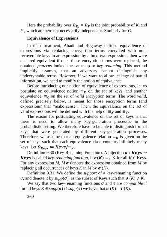
260

Here the probability over 𝛀𝑲𝒊 × 𝛀𝑭 is the joint probability of Ki and

F , which are here not necessarily independent. Similarly for G.

Equivalence of Expressions

In their treatment, Abadi and Rogaway defined equivalence of

expressions via replacing encryp-tion terms encrypted with non-

recoverable keys in an expression by a box; two expressions then were

declared equivalent if once these encryption terms were replaced, the

obtained patterns looked the same up to key-renaming. This method

implicitly assumes, that an adversary cannot distinguish any

undecryptable terms. However, if we want to allow leakage of partial

information, we need to modify the notion of equivalence.

Before introducing our notion of equivalence of expressions, let us

postulate an equivalence notion ≡𝑲 on the set of keys, and another

equivalence, ≡𝑪 on the set of valid encryption terms. The word valid,

defined precisely below, is meant for those encryption terms (and

expressions) that “make sense”. Then, the equivalence on the set of

valid expressions will be defined with the help of ≡𝑲 and ≡𝑪.

The reason for postulating equivalence on the set of keys is that

there is need to allow many key-generation processes in the

probabilistic setting. We therefore have to be able to distinguish formal

keys that were generated by different key-generation processes.

Therefore, we assume that an equivalence relation ≡𝑲 is given on the

set of keys such that each equivalence class contains infinitely many

keys. Let 𝑸𝑲𝒆𝒚𝒔 ≔ 𝑲𝒆𝒚𝒔/≡𝑲.

Definition 9.30 (Key-Renaming Function). A bijection 𝝈 ∶ 𝑲𝒆𝒚𝒔 →𝑲𝒆𝒚𝒔 is called key-renaming function, if 𝝈(𝑲) ≡𝑲 K for all K ∈ Keys.

For any expression M, M 𝝈 denotes the expression obtained from M by

replacing all occurrences of keys K in M by 𝝈 (K).

Definition 9.31. We define the support of a key-renaming function

𝜎, and denote it by supp(𝝈), as the subset of Keys such that 𝝈 (K) ≠ K.

We say that two key-renaming functions 𝝈 and 𝝉 are compatible if

for all keys K ∈ supp(𝝈) ∩ supp(𝝉) we have that 𝝈 (K) = 𝝉 (K).

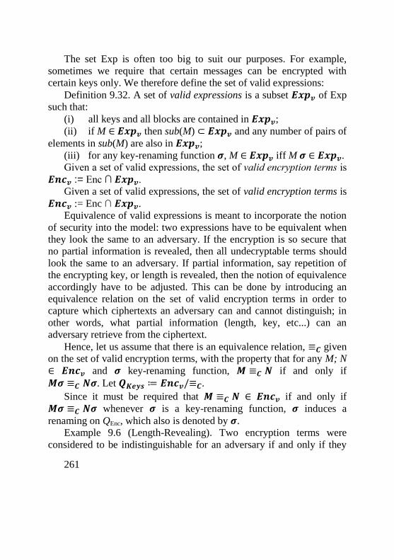
261

The set Exp is often too big to suit our purposes. For example,

sometimes we require that certain messages can be encrypted with

certain keys only. We therefore define the set of valid expressions:

Definition 9.32. A set of valid expressions is a subset 𝑬𝒙𝒑𝒗 of Exp

such that:

(i) all keys and all blocks are contained in 𝑬𝒙𝒑𝒗;

(ii) if M ∈ 𝑬𝒙𝒑𝒗 then sub(M) ⊂ 𝑬𝒙𝒑𝒗 and any number of pairs of

elements in sub(M) are also in 𝑬𝒙𝒑𝒗;

(iii) for any key-renaming function 𝝈, M ∈ 𝑬𝒙𝒑𝒗 iff M 𝝈 ∈ 𝑬𝒙𝒑𝒗.

Given a set of valid expressions, the set of valid encryption terms is

𝑬𝒏𝒄𝒗 := Enc ∩ 𝑬𝒙𝒑𝒗.

Given a set of valid expressions, the set of valid encryption terms is

𝑬𝒏𝒄𝒗 := Enc ∩ 𝑬𝒙𝒑𝒗.

Equivalence of valid expressions is meant to incorporate the notion

of security into the model: two expressions have to be equivalent when

they look the same to an adversary. If the encryption is so secure that

no partial information is revealed, then all undecryptable terms should

look the same to an adversary. If partial information, say repetition of

the encrypting key, or length is revealed, then the notion of equivalence

accordingly have to be adjusted. This can be done by introducing an

equivalence relation on the set of valid encryption terms in order to

capture which ciphertexts an adversary can and cannot distinguish; in

other words, what partial information (length, key, etc...) can an

adversary retrieve from the ciphertext.

Hence, let us assume that there is an equivalence relation, ≡𝑪 given

on the set of valid encryption terms, with the property that for any M; N

∈ 𝑬𝒏𝒄𝒗 and 𝝈 key-renaming function, 𝑴 ≡𝑪 𝑵 if and only if

𝑴𝝈 ≡𝑪 𝑵𝝈. Let 𝑸𝑲𝒆𝒚𝒔 ≔ 𝑬𝒏𝒄𝒗/≡𝑪.

Since it must be required that 𝑴 ≡𝑪 𝑵 ∈ 𝑬𝒏𝒄𝒗 if and only if

𝑴𝝈 ≡𝑪 𝑵𝝈 whenever 𝝈 is a key-renaming function, 𝝈 induces a

renaming on QEnc, which also is denoted by 𝝈.

Example 9.6 (Length-Revealing). Two encryption terms were

considered to be indistinguishable for an adversary if and only if they

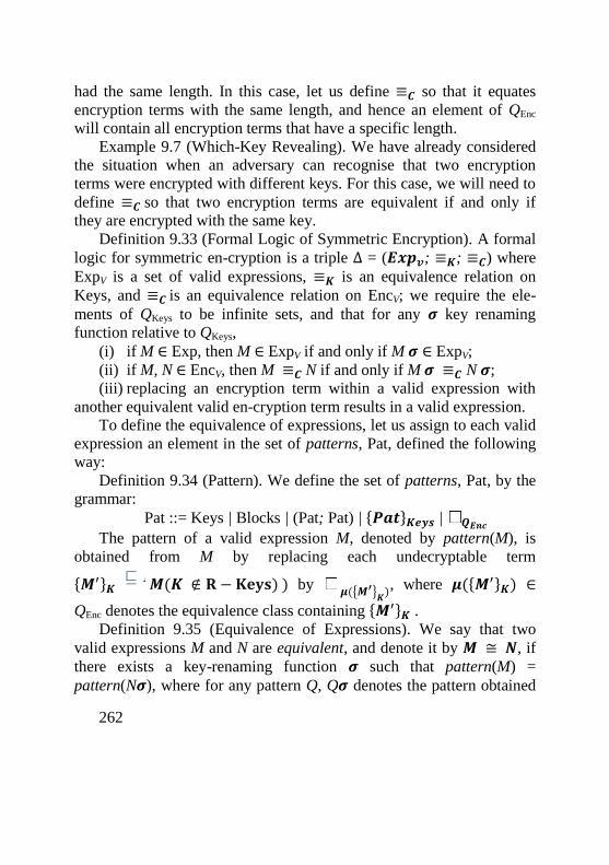
262

had the same length. In this case, let us define ≡𝑪 so that it equates

encryption terms with the same length, and hence an element of QEnc

will contain all encryption terms that have a specific length.

Example 9.7 (Which-Key Revealing). We have already considered

the situation when an adversary can recognise that two encryption

terms were encrypted with different keys. For this case, we will need to

define ≡𝑪 so that two encryption terms are equivalent if and only if

they are encrypted with the same key.

Definition 9.33 (Formal Logic of Symmetric Encryption). A formal

logic for symmetric en-cryption is a triple ∆ = (𝑬𝒙𝒑𝒗; ≡𝑲; ≡𝑪) where

ExpV is a set of valid expressions, ≡𝑲 is an equivalence relation on

Keys, and ≡𝑪 is an equivalence relation on EncV; we require the ele-

ments of QKeys to be infinite sets, and that for any 𝝈 key renaming

function relative to QKeys,

(i) if M ∈ Exp, then M ∈ ExpV if and only if M 𝝈 ∈ ExpV;

(ii) if M, N ∈ EncV, then M ≡𝑪 N if and only if M 𝝈 ≡𝑪 N 𝝈;

(iii) replacing an encryption term within a valid expression with

another equivalent valid en-cryption term results in a valid expression.

To define the equivalence of expressions, let us assign to each valid

expression an element in the set of patterns, Pat, defined the following

way:

Definition 9.34 (Pattern). We define the set of patterns, Pat, by the

grammar:

Pat ::= Keys | Blocks | (Pat; Pat) | {𝑷𝒂𝒕}𝑲𝒆𝒚𝒔 | 𝑸𝑬𝒏𝒄

The pattern of a valid expression M, denoted by pattern(M), is

obtained from M by replacing each undecryptable term

{𝑴′}𝑲 𝑴(𝑲 ∉ 𝐑 − 𝐊𝐞𝐲𝐬) ) by 𝝁({𝑴′}𝑲), where 𝝁({𝑴′}𝑲) ∈

QEnc denotes the equivalence class containing {𝑴′}𝑲 .

Definition 9.35 (Equivalence of Expressions). We say that two

valid expressions M and N are equivalent, and denote it by 𝑴 ≅ 𝑵, if

there exists a key-renaming function 𝝈 such that pattern(M) =

pattern(N𝝈), where for any pattern Q, Q𝝈 denotes the pattern obtained

263

by re-naming all the keys and the box-indexes (which are equivalence

classes in QEnc) in Q with 𝝈.

Example 9.8. In the case when the elements of QEnc contain

encryption terms encrypted with the same key, Example 9.7, there is a

one-to-one correspondence between QEnc and Keys, and therefore we

can index the boxes with keys instead of the elements in QEnc: 𝑲 , K

∈ Keys. Then if N is the same expression as in Example 9.3, the pattern

according to the above definition is the same as we had in that example.

In that example M and N are equivalent according to the definition of

equivalence above.

Proper Equivalence of Ciphers

In order to make the soundness and completeness proofs work, we

need to have some restrictions on ≡𝑪 ; without any restrictions, the

proofs will never work. The condition that we found the most natural

for our purposes is what we call proper equivalence, defined below.

This condition will make soundness work. For completeness, besides

proper equivalence, we need to assume something for the relationship

of ≡𝑪 and ≡𝑲 . We call our assumption independence, and it is defined

in Definition 2.37. Let us start by defining the set 𝝁𝒌𝒆𝒚, for each 𝝁 ∈

QEnc, as

𝝁𝒌𝒆𝒚 ∶= {𝑲 ∈ 𝐊𝐞𝐲𝐬 | 𝐭𝐡𝐞𝐫𝐞 𝐢𝐬 𝐚 𝐯𝐚𝐥𝐢𝐝 𝐞𝐱𝐩𝐫𝐞𝐬𝐬𝐢𝐨𝐧 𝑴

𝐬𝐮𝐜𝐡 𝐭𝐡𝐚𝐭 {𝐌}𝐊 ∈ 𝝁 }.

Definition 9.36 (Proper Equivalence of Ciphers). We say that an

equivalence relation ≡𝑪 on EncV is proper, if for any finite set of keys

S, if 𝝁 ∈ QEnc contains an element of the form {𝑵}𝑲 with K ∉ S, we

have that:

- if |𝝁𝒌𝒆𝒚| is finite then 𝝁 also contains an element C such that

Keys(C)∩S = ∅ , and K C;

- if |𝝁𝒌𝒆𝒚| = ∞ then 𝝁 also contains an element C such that

Keys(C) ∩ (S∪ {𝐊}) = ∅.

264

In other words, if 𝝁 contains an element encrypted with a key K not

in S, then 𝝁 has a representative in which no key of S appears, and in

which K may only appear as an encrypting key, but not as a

subexpression, or in the case of a class with infinitely many encrypting

keys there is an element in which no keys from S ∪ {𝐊} appear. In fact,

it was shown that the cardinality of the set 𝝁𝒌𝒆𝒚 is equal to either 1 or

∞.

Example 9.9. If ≡𝑪 denotes the equivalence of Example 2.7 (i.e.

two ciphers are equivalent if they have the same encrypting key, hence

|𝝁𝒌𝒆𝒚| = 1), then it is clearly proper, since if {𝑴}𝑲 ∈ 𝝁, and K ∉ S,

then C = {𝑲′}𝑲 works for any K' ∉ S; there is such a K', since we

assumed that there are infinitely many keys. C = {𝑩}𝑲 (B ∈ Blocks) is

also a good choice since Blocks is not empty.

Example 9.10. If ≡𝑪 denotes the equivalence of Example 2.6, then

it is clearly proper (|𝝁𝒌𝒆𝒚|=∞). If {𝑴}𝑲 ∈ 𝝁, K ∉ S, then C = {𝑴′}𝑲′ is

a good choice where C is constructed by assigning to each key in {𝑴}𝑲,

a new key K'' not in S ∪ {𝐊}. We can do this since we assumed that

there are infinitely many keys. Then, since key-renaming does not

change the length, l(M) = l (M'), and 𝝁 contains all encryption terms of

the same length, C ∈ 𝝁 and properness follows.

The following propositions will be useful for proving our general

soundness and complete-ness results.

Proposition 9.1. Let ∆ = (ExpV; ≡𝑲 ; ≡𝑪 ) be such that ≡𝑪 is

proper. Then, the equivalence relation ≡𝑪 is such that for any

equivalence class 𝝁 ∈ QEnc, 𝝁 key has either one, or infinitey many

elements.

Proof. Let 𝝁 ∈ QEnc, and assume that there are more than one

encrypting key in 𝝁 key (but |𝝁𝒌𝒆𝒚| finite), that is, there are two different

keys K and K1 such that {𝑴}𝑲, {𝑴𝟏}𝑲𝟏 ∈ 𝝁 for some valid expressions

M and M1. Since ≡𝑪 ) is proper and {𝑴𝟏}𝑲𝟏 ∈ 𝝁, if we consider S =

{𝑲}(𝑲𝟏 ≠ 𝑲 𝐭𝐡𝐮𝐬 𝑲𝟏 ∉ 𝐒) then 𝝁 has an element of the form {𝑴′}𝑲′

265

in which no key of S appears and in which K1 may only appear as an

encrypting key, but not as a subexpression. In particular we have that

𝑲 ∉ 𝑲𝒆𝒚𝒔(𝑴′)𝒂𝒏𝒅𝑲 ≠ 𝑲′ Since we assumed that each equivalence class in QKeys contains

infinitely many elements (recall Definition 2.33), there is a key L ≠ K

such that L ≡𝑲 K, and 𝑳 ∉ 𝐊𝐞𝐲𝐬({𝐌}𝐊) ∪ 𝐊𝐞𝐲𝐬({𝐌′}𝐊′).

Then, defining 𝝈 to do nothing else but to switch the keys L and K,

we have using (2.2) that

{𝑀}𝑲𝝈 = {𝑴𝝈}𝑳 and (by (2.1) and (2.2)) {𝑴′}𝑲′𝝈 = {𝑴′}𝑲′

But, since {𝑴}𝑲 ≡𝑪 {𝑴′}𝑲′, we have (by definition of formal logic)

that

{𝑴}𝑲𝝈 ≡𝑪 {𝑴′}𝑲′𝝈

that is

{𝑴𝝈}𝑳 ≡𝑪 {𝑴′}𝑲′ Since {𝑴′}𝑲′ ∈ 𝝁, it must hold that {𝑴𝝈}𝑳 ∈ 𝝁. Therefore, there

are infinitely many encrypting keys in 𝝁 since there are infinitely many

choices for L.

Proposition 9.2. Let ∆= (𝑬𝒙𝒑𝒗, ≡𝑲, ≡𝑪) be such that ≡𝑪 is proper.

If 𝝈 is a key-renaming function (relative to ≡𝑲), then for any 𝝁 ∈

𝑸𝑬𝒏𝒄, |𝝁𝒌𝒆𝒚| = |𝝈(𝝁)𝒌𝒆𝒚|.

Proof. If |𝝁𝒌𝒆𝒚| = ∞, then|𝝈(𝝁)𝒌𝒆𝒚| = ∞, since for any {𝑴}𝑲 ∈ 𝝁,

{𝑴}𝑲𝝈 = {𝑴𝝈}𝝈(𝑲) ∈ 𝝈(𝝁). Since 𝝈 is a bijection, and since any 𝝁

contains either only one or infinitely many elements, the claim follows.

The meaning of the next proposition is that if ≡𝑪 is proper, then

given a set of valid ciphers 𝑪 = {{𝑵𝒊}𝑳𝒊}𝒊=𝟏𝒏

such that none of the

encrypting keys are in S, and if 𝝁𝟏, … , 𝝁𝒍 are all the equivalence classes

of the elements in C, then it is possible to choose a representative of

each of 𝝁𝒋, denoted by 𝑪𝝁𝒋 , such that no key of S occurs in any of 𝑪𝝁𝒋 ,

none of the Li’s occur as a subexpression in any 𝑪𝝁𝒋, and no key occurs

in two of 𝑪𝝁𝒋unless the corresponding two equivalence classes both

have only the same, single encrypting key.

266

Proposition 9.3. Let ∆ = (𝑬𝒙𝒑𝒗, ≡𝑲, ≡𝑪)) be such that ≡𝑪 is

proper. Let 𝑪 = {{𝑵𝒊}𝑳𝒊}𝒊=𝟏𝒏

be a set of valid encryption terms, and S a

finite set of keys with 𝑳𝒊 ∉ 𝐒(𝐢 ∈ {𝟏,… , 𝐧}). Let 𝝁( ) denote the set of

all equivalence-classes with respect to ≡𝑪 of all elements in . Then,

for each 𝒗 ∈ 𝝁( ), there is an element 𝑪𝒗 ∈ 𝒗 such that:

98. Keys(𝑪𝒗) ∩ 𝐒 = ∅

99. 𝑳𝒊 𝑪𝒗 for all 𝒊 ∈ {𝟏,… , 𝒏}

100. 𝒊𝒇 𝒗 ≠ 𝒗′|𝒗𝒌𝒆𝒚| ≠ ∞ 𝒂𝒏𝒅 |𝒗′𝒌𝒆𝒚| ≠ ∞, then Keys(𝑪𝒗 ) ∩

Keys(𝑪𝒗′) = ∅ ; if and only if 𝒗𝒌𝒆𝒚 = 𝒗′𝒌𝒆𝒚 {𝑲} for some key

K, and in this case:

- Keys(𝑪𝒗 ) ∩Keys(𝑪𝒗′) = {𝑲} , - 𝑪𝒗 and 𝑪𝒗′ are both of the form {•}𝑲 with the same K, and

- K 𝑪𝒗 , K 𝑪𝒗′.

101. if 𝒗 ≠ 𝒗′ and either |𝒗𝒌𝒆𝒚| = ∞ or |𝒗′𝒌𝒆𝒚| = ∞, then

Keys(𝑪𝒗 ) ∩Keys(𝑪𝒗′)) = ∅.

Proof. Observe, that if 𝝁𝒊 denotes the equivalence class of {𝑵𝒊}𝑳𝒊 in

QEnc, then v ∈ 𝝁(𝑪) if and only if v = 𝝁𝒊 for some ∈ {𝟏,…𝒏} . Proof

goes by induction.

The statement is clearly true if n = 1, since ≡𝑪 is proper.

Suppose now that the result is true for n - 1. Let {𝑵𝟏}𝑳𝟏 , {𝑵𝟐}𝑳𝟐 ,...,

{𝑵𝒏}𝑳𝒏 be valid expressions, and let S be a set of keys such that Li ∉ S.

Without loss of generality, we can assume, that the numbering is such

that there is an , 𝟏 ≤ 𝒍 ≤ 𝒏 , such that |(𝝁𝒊)𝒌𝒆𝒚| if 𝒊 ≤ 𝒍 and

|(𝝁𝒊)𝒌𝒆𝒚| = ∞ 𝒊𝒇 > 𝒍.

Case 9.1: Let us first assume that l = n, i.e., |(𝝁𝒊)𝒌𝒆𝒚| = 𝟏 for all

𝟏 ≤ 𝒊 ≤ 𝒏 , and that there is an 𝒎 ∈ {𝟏,… , 𝒏 − 𝟏} such that Ln = Lm.

Since the statement is assumed to be true for n-1 , we have that for the

267

family of encryption terms

′

{{𝑵𝒊}𝑳𝒊}𝒊=𝟏𝒏−𝟏

and the set S we can

choose 𝑪𝝁𝒊 for all 𝒊 ≤ 𝒏 − 𝟏 such that conditions (i'), (ii'), (iii') and (iv')

hold for these , that is,

(i') Keys(𝑪𝝁𝒊) ⋂ S = ∅; for all 𝟏 ≤ 𝒊, 𝒋 ≤ 𝒏 − 𝟏 ,

(ii') 𝑳𝒊 𝑪𝝁𝒋 for all 𝟏 ≤ 𝒊, 𝒋 ≤ 𝒏 − 𝟏 , and

(iii') if 𝝁𝒊 ≠ 𝝁𝒋 , |(𝝁𝒊)𝒌𝒆𝒚| ≠ ∞ and |(𝝁𝒋)𝒌𝒆𝒚|≠ ∞, then

𝑲𝒆𝒚𝒔(𝑪𝝁𝒊) ⋂ 𝑲𝒆𝒚𝒔(𝑪𝝁𝒋) ≠ ∅ ; if and only if (𝝁𝒊)𝒌𝒆𝒚 = (𝝁𝒋)𝒌𝒆𝒚 =

{𝑲} for some key K, and in that case

102. 𝑲𝒆𝒚𝒔(𝑪𝝁𝒊) ⋂ 𝑲𝒆𝒚𝒔(𝑪𝝁𝒋) = {𝑲},

103. 𝑪𝝁𝒊 and 𝑪𝝁𝒋 are both of the form {•}𝑲 with the same K,

and

104. 𝑲 𝑪𝝁𝒊 , 𝑲 𝑪𝝁𝒋.

(iv') if 𝝁𝒊 ≠ 𝝁𝒋 and either |(𝝁𝒊)𝒌𝒆𝒚| = ∞ or |(𝝁𝒋)𝒌𝒆𝒚| = ∞, then

𝑲𝒆𝒚𝒔(𝑪𝝁𝒊) ⋂ 𝑲𝒆𝒚𝒔(𝑪𝝁𝒋) = ∅ .

We can immediately discard (iv') since we suppose that |(𝝁𝒊)𝒌𝒆𝒚| =

𝟏 for all 𝟏 ≤ 𝒊 ≤ 𝒏. Suppose now that 𝝁𝒏 = 𝝁𝒋 for some 𝒊 ≤ 𝒏 − 𝟏,

then there is nothing to prove, 𝑪𝝁𝒏 = 𝑪𝝁𝒊 has already been chosen and

so (i), (ii) and (iii) are obviously satisfied by IH.

If there is no such i, then consider

𝑺𝒏−𝟏 ≔ ((⋃𝑲𝒆𝒚𝒔(𝑪𝝁𝒊) ∪

𝒏−𝟏

𝒊=𝟏

{𝑳𝒊})\{𝑳𝒏}) ∪ 𝑺

Since ≡𝑪 is proper (using 𝑺𝒏−𝟏 and {𝑵𝒏}𝑳𝒏 ∈ 𝝁𝒏 ), there is a

𝑪 ∈ 𝝁𝒏 such that 𝑲𝒆𝒚𝒔(𝑪) ∪ 𝑺𝒏−𝟏 = ∅ and 𝑳𝒏 𝑪. Let us define

𝑪𝝁𝒏 = 𝑪. Then:

(i) 𝑲𝒆𝒚𝒔(𝑪)⋂𝑺 = ∅ ; follows from the fact that

𝑲𝒆𝒚𝒔(𝑪) ⋂ 𝑺𝒏−𝟏 = ; and 𝑺 ⊆ 𝑺𝒏−𝟏 ;

268

(ii) 𝑳𝒊 𝑪𝝁𝒋 for all 𝟏 ≤ 𝒊, 𝒋 ≤ 𝒏 since:

1. 𝑳𝒊 𝑪𝝁𝒋 , for all 𝟏 ≤ 𝒊, 𝒋 ≤ 𝒏 − 𝟏 by (ii'),

2. 𝑳𝒏 𝐶𝝁𝒋 , 𝟏 ≤ 𝒋 ≤ 𝒏 − 𝟏 because we assumed that Ln = Lm

and 𝑳𝒎 𝑪𝝁𝒋 by (ii'),

3. 𝑳𝒊 𝑪, for all 𝑳𝒊 ≠ 𝑳𝒎 such that 𝟏 ≤ 𝒊 ≤ 𝒏 − 𝟏 (remember

that Ln = Lm) since 𝑳𝒊 ∈ 𝑺𝒏−𝟏 and 𝑲𝒆𝒚𝒔(𝑪) ⋂ 𝑺𝒏−𝟏 = ∅,

and

4. 𝑳𝒏 𝑪 by the way that C was chosen (hence 𝑳𝒎 𝑪).

(iii)

1. for all 𝟏 ≤ 𝒊, 𝒋 ≤ 𝒏 − 𝟏 it is true by (iii');

2. Suppose now that 𝝁𝒏 ≠ 𝝁𝒌 and (𝑪) ⋂ 𝑲𝒆𝒚𝒔(𝑪𝝁𝒌) ≠ ∅ ;

for some 𝟏 ≤ 𝒌 ≤ 𝒏 − 𝟏. If we combine these with the fact

that 𝑲𝒆𝒚𝒔(𝑪) ⋂ 𝑺𝒏−𝟏 = ∅, we need to have that

𝑲𝒆𝒚𝒔(𝑪) ⋂ 𝑲𝒆𝒚𝒔(𝑪𝝁𝒌) = {𝑳𝒏}.

It is now easy to see from the equation above that C and 𝑪𝝁𝒌 are

both of the form {•}𝑳𝒏. For that notice that by (ii.d) just proved above,

𝑳𝒏 𝑪 and by (ii.a) 𝑳𝒏 𝑪𝝁𝒌. The only thing left to show is that

(𝝁𝒏)𝒌𝒆𝒚 = (𝝁𝒌)𝒌𝒆𝒚 = {𝑳𝒏} . This comes straightforward from the fact

that C and 𝑪𝝁𝒌are both of the form {•}𝑳𝒏 and from the fact that

|(𝝁𝒊)𝒌𝒆𝒚| = 𝟏 for all 𝟏 ≤ 𝒊 ≤ 𝒏. Combining these we have

(𝝁𝒏)𝒌𝒆𝒚 = (𝝁𝒌)𝒌𝒆𝒚 = {𝑳𝒏}.

The converse is very simple. Suppose that (𝝁𝒏)𝒌𝒆𝒚 = (𝝁𝒌)𝒌𝒆𝒚 =

{𝑳𝒏}. Since 𝑪 ∈ 𝝁𝒏 and 𝑪𝝁𝒌 ∈ 𝝁𝒌 we have that both are of the form

{•}𝑳𝒏 and thus 𝑲𝒆𝒚𝒔(𝑪) ⋂ 𝑲𝒆𝒚𝒔(𝑪𝝁𝒌) ≠ ∅. The rest follows as

above.

(iv) Verified since by hypothesis we suppose that |(𝝁𝒊)𝒌𝒆𝒚| = 𝟏 for

all 𝟏 ≤ 𝒊 ≤ 𝒏.

269

Case 9.2: Suppose now that l = n, but there is no 𝒎 ∈ {𝟏,… , 𝒏 − 𝟏} such that Ln = Lm. Since the result is true for n-1, we have that for the

family of encryption terms '{{𝑵𝒊}𝑳𝒊}𝒊=𝟏𝒏−𝟏

and the set 𝑺′ = 𝑺 ∪ {𝑳𝒏}

(note that 𝑳𝒊 ∉ 𝑺′ for all 𝒊 ≤ 𝒏 − 𝟏) we can choose 𝑪𝝁𝒊 for all 𝒊 ≤ 𝒏 −

𝟏 such that conditions (i'), (ii'), (iii') and (iv') hold for these , that is,

(i') Keys(𝑪𝝁𝒊)⋂(𝑺 ∪ {𝑳𝒏}) = ∅ for all 𝟏 ≤ 𝒊 ≤ 𝒏 − 𝟏,

(ii') 𝑳𝒊 𝑪𝝁𝒋 for all 𝟏 ≤ 𝒊, 𝒋 ≤ 𝒏 − 𝟏, and

(iii') if 𝝁𝒊 ≠ 𝝁𝒋, |(𝝁𝒊)𝒌𝒆𝒚| ≠ ∞ and |(𝝁𝒋)𝒌𝒆𝒚|≠ ∞, then

𝑲𝒆𝒚𝒔(𝑪𝝁𝒊) ⋂ 𝑲𝒆𝒚𝒔(𝑪𝝁𝒋) ≠ ∅ if and only if (𝝁𝒊)𝒌𝒆𝒚 = (𝝁𝒋)𝒌𝒆𝒚= {𝑲}

for some key K;

(iv') if 𝝁𝒊 ≠ 𝝁𝒋 and either |(𝝁𝒊)𝒌𝒆𝒚| = ∞ or |(𝝁𝒋)𝒌𝒆𝒚| = ∞, then

𝑲𝒆𝒚𝒔(𝑪𝝁𝒊) ⋂𝑲𝒆𝒚𝒔 (𝑪𝝁𝒋) = ∅.

Again, if 𝝁𝒏 = 𝝁𝒊 for some i < n, then there is nothing to prove, let

𝑪𝝁𝒏 = 𝑪𝝁𝒊 and note that (i) and (iii) are obviously satisfied, and (ii)

(𝑳𝒏 𝑪𝝁𝒋 , for all 𝟏 ≤ 𝒋 ≤ 𝒏, and 𝑳𝒊 𝑪𝝁𝒏 for all 𝟏 ≤ 𝒊 ≤ 𝒏 − 𝟏)

follows from (i') and (ii') respectively. Again (iv) is also true since we

suppose that |(𝝁𝒊)𝒌𝒆𝒚| = 𝟏 for all 𝟏 ≤ 𝒊 ≤ 𝒏.

If there is no such i, then consider

𝑺𝒏−𝟏(⋃𝑲𝒆𝒚𝒔(𝑪𝝁𝒊) ∪ {𝑳𝒊}

𝒏−𝟏

𝒊=𝟏

) ∪ 𝐒.

By properness (using 𝑺𝒏−𝟏 and {𝑵𝒏}𝑳𝒏 ∈ 𝝁𝒏), and since 𝑳𝒏 ∉ 𝑺𝒏−𝟏

(by (i') assumption 𝑳𝒏 ≠ 𝑳𝒊 for all i < n, and by hypothesis of the

proposition 𝑳𝒏 ∉ 𝐒), there is a 𝑪 ∈ 𝝁𝒏 such that 𝑲𝒆𝒚𝒔(𝑪)⋂𝑺𝒏−𝟏 = ∅,

and 𝑳𝒏 𝑪. Let us define 𝑪𝝁𝒏 = 𝑪. Then:

(i)follows from (i') and from the fact that 𝑲𝒆𝒚𝒔(𝑪)⋂𝑺𝒏−𝟏 = ∅;

(ii) is true, since:

270

1. 𝑳𝒊 𝑪𝝁𝒋 , for all 𝟏 ≤ 𝒊, 𝒋 ≤ 𝒏 − 𝟏 by (ii'),

2. 𝑳𝒏 𝑪𝝁𝒋 , for all 𝟏 ≤ 𝒋 ≤ 𝒏 − 𝟏 by (i'),

3. 𝑳𝒊 𝑪 for 𝟏 ≤ 𝒊 ≤ 𝒏 − 𝟏 because by properness

𝑲𝒆𝒚𝒔(𝑪)⋂𝑺𝒏−𝟏 = ∅, and

4. 𝑳𝒏 𝑪 because of properness.

(iii) follows, because:

1. for all 𝟏 ≤ 𝒊, 𝒋 ≤ 𝒏 − 𝟏 it is true by (iii'), and

2. for the other case it holds since by properness

𝑲𝒆𝒚𝒔(𝑪)⋂𝑺𝒏−𝟏 = ∅ and thus 𝑲𝒆𝒚𝒔(𝑪)⋂ 𝑲𝒆𝒚𝒔(𝑪𝝁𝒊) =

∅ for all 𝒊 ≤ 𝒊 ≤ 𝒏 − 𝟏.

(iv)Verified since by hypothesis we suppose that |(𝝁𝒊)𝒌𝒆𝒚| = 𝟏 for

all 𝟏 ≤ 𝒊 ≤ 𝒏.

Case 9.3: Suppose now that l < n, but there is 𝒎 ∈ {𝟏,… , 𝒏 − 𝟏} such that Ln = Lm. Since the result is assumed to be true for n - 1, we

have that for the family of encryption terms ′ = {{𝑵𝒊}𝑳𝒊}𝒊=𝟏

𝒏−𝟏

and the

set S we can choose 𝑪𝝁𝒊 for all 𝒊 ≤ 𝒏 − 𝟏 such that conditions (i'), (ii'),

(iii') and (iv') hold for these , that is,

(i') Keys(𝑪𝝁𝒊) ⋂ S = ∅ for all 𝟏 ≤ 𝒊 ≤ 𝒏 − 𝟏,

(ii') 𝑳𝒊 𝑪𝝁𝒋 for all 𝟏 ≤ 𝒊, 𝒋 ≤ 𝒏 − 𝟏, and

(iii') if 𝝁𝒊 ≠ 𝝁𝒋, |(𝝁𝒊)𝒌𝒆𝒚| ≠ ∞ 𝒂𝒏𝒅 |(𝝁𝒋)𝒌𝒆𝒚|≠ ∞, then Keys(𝑪𝝁𝒊)

⋂ Keys(𝑪𝝁𝒋) ≠ ∅ if and only if (𝝁𝒊)𝒌𝒆𝒚 = (𝝁𝒋)𝒌𝒆𝒚= {𝑲} for some key

K;

(iv') if 𝝁𝒊 ≠ 𝝁𝒋 and either |(𝝁𝒊)𝒌𝒆𝒚| = ∞ or |(𝝁𝒋)𝒌𝒆𝒚|= ∞, then

Keys(𝑪𝝁𝒊) ⋂ Keys(𝑪𝝁𝒋) = ∅.

271

Again, suppose now that 𝝁𝒏 = 𝝁𝒊 for some 𝒊 ≤ 𝒏 − 𝟏, then there is

nothing to prove, 𝑪𝝁𝒏 =has already been chosen and so (i), (ii), (iii) and

(iv) are obviously satisfied by IH.

If there is no such i, then consider

𝑺𝒏−𝟏 ≔ ((⋃𝑲𝒆𝒚𝒔(𝑪𝝁𝒊 ) ∪ {𝑳𝒊})\{𝑳𝒏}) ∪ 𝑺

𝒏−𝟏

𝒊=𝟏

Since ≡𝑪 is proper (using 𝑺𝒏−𝟏 and {𝑵𝒏}𝑳𝒏 ∈ 𝝁𝒏, |(𝝁𝒏)𝒌𝒆𝒚| = ∞),

there is a 𝑪 ∈ 𝝁𝒏 such that Keys(C) ∩ (𝑺𝒏−𝟏 ∪ {𝑳𝒏}) = ∅. Then:

(i) Keys(C) ∩ 𝑺 = ∅ follows from the fact that Keys(C)∩ ( 𝑺𝒏−𝟏 ∪{𝑳𝒏}) = ∅ and S ⊆ ( 𝑺𝒏−𝟏 ∪ {𝑳𝒏});

(ii) 𝑳𝒊 𝑪𝝁𝒋for all 𝟏 ≤ 𝒊, 𝒋 ≤ 𝒏 since:

1. 𝑳𝒏 𝑪𝝁𝒋 , for all 𝟏 ≤ 𝒊, 𝒋 ≤ 𝒏 − 𝟏 by (ii'),

2. 𝑳𝒏 𝑪𝝁𝒋 , 𝟏 ≤ 𝒋 ≤ 𝒏 − 𝟏 because we assumed that Ln =

Lm and Lm 𝑪𝝁𝒋 by (ii'),

3. 𝑳𝒊 𝑪, for all Li ≠ 𝑳𝒎 such that 𝟏 ≤ 𝒊 ≤ 𝒏 − 𝟏

(remember that Ln = Lm) since 𝑳𝒊 ∈ 𝑺𝒏−𝟏 and Keys(C)∩𝑺𝒏−𝟏 = ∅, and

4. 𝑳𝒏 𝑪 because Keys(C) ∩ (𝑺𝒏−𝟏 ∪ {𝑳𝒏}) = ∅ (hence

𝑳𝒎 𝑪).

(iii) note that if |(𝝁𝒊)𝒌𝒆𝒚| ≠ ∞ 𝒂𝒏𝒅 |(𝝁𝒋)𝒌𝒆𝒚| ≠ ∞ then 𝟏 ≤ 𝒊, 𝒋 ≤

𝒍 < 𝒏 and thus by HI (iii) holds.

(iv)

1. for the case 𝒍 ≤ 𝒋 ≤ 𝒏 − 𝟏 and 𝟏 ≤ 𝒊 ≤ 𝒏 − 𝟏,

Keys(𝑪𝝁𝒋) ∩ Keys(𝑪𝝁𝒊)= ∅ holds by IH;

2. it is only left to show that for all 𝟏 ≤ 𝒊 ≤ 𝒏 − 𝟏,

Keys(𝑪𝝁𝒏) ∩Keys(𝑪𝝁𝒊) = ∅. This is true because by

272

definition Keys(𝑪𝝁𝒏) ∩ (𝑺𝒏−𝟏 ∪ {𝑳𝒏}) = ∅ and Keys(𝑪𝝁𝒊))

⊆ (𝑺𝒏−𝟏 ∪ {𝑳𝒏})).

Case 9.4: The proof of the remaining case, l < n, i.e., |(𝝁𝒊)𝒌𝒆𝒚| =

∞ for l < i ≤ n, and there is no 𝒎 ∈ {𝟏,… , 𝒏 − 𝟏} such that Ln = Lm is a

combination of the proofs of Case 2 and Case 3. Since the result is true

for 𝒏 − 𝟏, we have that for the family of encryption terms ′

{{𝑵𝒊}𝑳𝒊}𝒊=𝟏𝒏−𝟏

and the set 𝑺′ = 𝑺 ∪ {𝑳𝒏} (note that 𝑳𝒊 ∉ 𝑺′ for all i

≤ 𝒏 − 𝟏 ) we can choose 𝑪𝝁𝒊 for all i ≤ 𝒏 − 𝟏 such that conditions (i'),

(ii'), (iii') and (iv') hold for these , that is,

(i') Keys(𝑪𝝁𝒊) ∩ (𝑺 ∪ {𝑳𝒏}) = ∅ for all 1 ≤ 𝒊 ≤ 𝒏 − 𝟏;

(ii') 𝑳𝒏 𝑪𝝁𝒋 for all 1 ≤ 𝒊, 𝒋 ≤ 𝒏 − 𝟏, and

(iii') if 𝝁𝒊 ≠ 𝝁𝒋, |(𝝁𝒊)𝒌𝒆𝒚| ≠ ∞ and |(𝝁𝒋)𝒌𝒆𝒚|≠ ∞, then

Keys(𝑪𝝁𝒊) ∩ Keys(𝑪𝝁𝒋) ≠ ∅ if and only if (𝝁𝒊)𝒌𝒆𝒚 = (𝝁𝒋)𝒌𝒆𝒚= {𝑲} for

some key K;

(iv') if 𝝁𝒊 ≠ 𝝁𝒋 and either |(𝝁𝒊)𝒌𝒆𝒚| = ∞ or |(𝝁𝒊)𝒌𝒆𝒚| = ∞ , then

Keys(𝑪𝝁𝒊) ∩ Keys(𝑪𝝁𝒋) = ∅.

Again, if 𝝁𝒏 = 𝝁𝒊 for some i < n, then there is nothing to prove, let

𝑪𝝁𝒏 = 𝑪𝝁𝒊 and note that (i), (iii) and (iv) are obviously satisfied, and (ii)

(𝑳𝒏 𝑪𝝁𝒋 , for all 1 ≤ 𝒋 ≤ 𝒏, and 𝑳𝒊 𝑪𝝁𝒏 for all 1 ≤ 𝒊 ≤ 𝒏 − 𝟏)

follows from (i') and (ii') respectively.

If there is no such i, then consider

𝑺𝒏−𝟏 ≔ ((⋃𝑲𝒆𝒚𝒔(𝑪𝝁𝒊 ) ∪ {𝑳𝒊}) ∪ 𝑺

𝒏−𝟏

𝒊=𝟏

By properness (using 𝑺𝒏−𝟏 and {𝑵𝒏}𝑳𝒏 ∈ 𝝁𝒏, |(𝝁𝒏)𝒌𝒆𝒚| = ∞), and

since 𝑳𝒏 ∉ 𝑺𝒏−𝟏 (by (i'), assumption 𝑳𝒏 ≠ 𝑳𝒊 for all i < n, and by

hypothesis of the proposition Ln ∉ 𝑺), there is a 𝑪 ∈ 𝝁𝒏 such that

Keys(C) ∩ (𝑺𝒏−𝟏 ∩ {𝑳𝒏}) = ∅. Let us define 𝑪𝝁𝒏 = C. Then:

273

(i) follows from (i') and from the fact that Keys(C) ∩ 𝑺𝒏−𝟏 = ∅;

(ii) is true, since:

1. 𝑳𝒊 𝑪𝝁𝒋 , for all 1 ≤ 𝒊, 𝒋 ≤ 𝒏 − 𝟏 by (ii'),

2. 𝑳𝒏 𝑪𝝁𝒋 , for all 1 ≤ 𝒋 ≤ 𝒏 − 𝟏 by (i'),

3. 𝑳𝒊 𝑪 for 1 ≤ 𝒊 ≤ 𝒏 − 𝟏 because by properness

Keys(C) ∩ 𝑺𝒏−𝟏 = ∅, and

4. 𝑳𝒏 𝑪 because by definition of C, Keys(C) ∩ 𝑺𝒏−𝟏

∪ {𝑳𝒏} = ∅.

(iii) note that if |(𝝁𝒊)𝒌𝒆𝒚| ≠ ∞), and |(𝝁𝒋)𝒌𝒆𝒚| ≠ ∞), then 1

≤ 𝒊, 𝒋 ≤ 𝒍 < 𝒏 and thus by HI (iii) holds.

(iv)

1. for the case l ≤ 𝒋 ≤ 𝒏 − 𝟏 and 1 ≤ 𝒊 ≤ 𝒏 − 𝟏, Keys(𝑪𝝁𝒋) ∩

Keys(𝑪𝝁𝒊) = ∅ holds by IH;

2. it is only left to show that for all 1 ≤ 𝒊 ≤ 𝒏 − 𝟏,

Keys(𝑪𝝁𝒏) ∩Keys(𝑪𝝁𝒊) = ∅. This is true because by

definition Keys(𝑪𝝁𝒏) ∩ (𝑺𝒏−𝟏 ∪ {𝑳𝒏}) = ∅ and Keys(𝑪𝝁𝒊)

⊆ 𝑺𝒏−𝟏.

Given sets C and s as iin the conditions og the proposition, let

R(C,S) denote the nonempty set

conditionssatisfySandCandvCCSCR Cvvv

Cvv

,|:),(

)(

Another useful property satisfied by all common logics, and that we

will need for the completeness result is the following:

Definition 9.37 (Independent ≡𝑲 and ≡𝑪). We say that ≡𝑲 and ≡𝑪

are independent, if for any finite set of keys S, and any finite set of

ciphers C such that no key in S appears in any element of C, given any

key-renaming function 𝝈, there is a key renaming 𝝈' for which 𝝈'(K) =

K whenever 𝑲 ∈ 𝑺, and for all C ∈ C, C 𝝈 ≡𝑪 C 𝝈'.

274

In other words, ≡𝑲 and ≡𝑪 are independent, if for any finite set of

keys S, and any finite set of ciphers C such that no key in S appears in

any element of C, it is possible to alter any key-renaming function 𝝈

such that the altered function leaves all the elements in S unchanged,

whereas on C it does the same thing as the original 𝝈. We will need this

property for the general completeness theorem.

9.5.3 Interpretation

The idea of the interpretation is to describe messages that are built

from blocks of strings and keys via pairing and encryption. To each

valid formal expression M, the interpretation assigns a random variable

Φ(M) taking values in 𝒔𝒕𝒓𝒊𝒏𝒈𝒔̅̅ ̅̅ ̅̅ ̅̅ ̅̅ ̅. We do not give one specific

interpreting function though, we will just say that a function Φ is an

interpretation if it satisfies certain properties. Let us assume, that a

function ∅ is fixed in advance, which assigns to each formal key a key-

generation algorithm. If Φ (B) ∈ 𝒔𝒕𝒓𝒊𝒏𝒈𝒔̅̅ ̅̅ ̅̅ ̅̅ ̅̅ ̅ (constant random variable) is

given for blocks, then, the rest of Φ is determined the following way:

First, run the key-generation algorithm assigned by ∅ for each key in

Keys(M). Then, using the outputs of these key-generations, translate the

formal expressions according to the following rules: for each key, use

the output of the corresponding key-generation. For blocks, just use

Φ(B). For each pair, apply [• ; •] to the interpretations of the

expressions inside the formal pair. For each formal encryption, run the

encryption algorithm using as key the bitstring that was output by the

key generation, to encrypt the interpretation of the formal expression

inside the formal encryption. The randomness of Φ (M) comes from the

initial key-generation, and from running the encryption algorithm

independently for each formal encryption. Let us define below this

notion of interpretation with the following example:

Example 9.11. For M = (({𝟎}𝑲𝟏𝟎,𝑲𝟓), {𝑲𝟏𝟎}𝑲𝟓), the interpretation

is Φ(M):(𝛀𝑬 ×𝛀𝑬) × (𝛀𝚽(𝐊𝟓) ×𝛀𝚽(𝐊𝟏𝟎)) → 𝒔𝒕𝒓𝒊𝒏𝒈𝒔̅̅ ̅̅ ̅̅ ̅̅ ̅̅ ̅, where

𝜱(𝑴)(𝝎𝟏, 𝝎𝟐, 𝝎𝟑, 𝝎𝟒) is

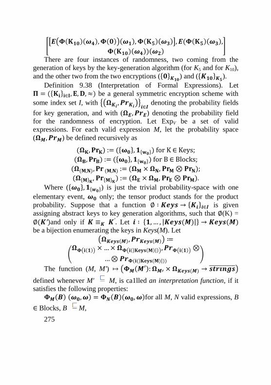
275

[[𝑬(𝚽(𝐊𝟏𝟎)(𝝎𝟒),𝚽(𝟎))(𝝎𝟏),𝚽(𝐊𝟓)(𝝎𝟑)], 𝑬(𝚽(𝐊𝟓)(𝝎𝟑),

𝚽(𝐊𝟏𝟎)(𝝎𝟒))(𝝎𝟐)]

There are four instances of randomness, two coming from the

generation of keys by the key-generation algorithm (for K5 and for K10),

and the other two from the two encryptions ({𝟎}𝑲𝟏𝟎) and ({𝑲𝟏𝟎}𝑲𝟓).

Definition 9.38 (Interpretation of Formal Expressions). Let

𝚷 = ({𝐊𝐢}𝐢∈𝐈, 𝐄, 𝐃, ≈) be a general symmetric encryption scheme with

some index set I, with {(𝛀𝑲𝒊 , 𝑷𝒓𝑲𝒊)}𝒊∈𝑰 denoting the probability fields

for key generation, and with (𝛀𝑬, 𝑷𝒓𝑬) denoting the probability field

for the randomness of encryption. Let ExpV be a set of valid

expressions. For each valid expression M, let the probability space

(𝛀𝑴, 𝑷𝒓𝑴) be defined recursively as

(𝛀𝐊, 𝐏𝐫𝐊) := ({𝛚𝟎}, 𝟏{𝐰𝟎}) for K ∈ Keys;

(𝛀𝐁, 𝐏𝐫𝐁) := ({𝛚𝟎}, 𝟏{𝐰𝟎}) for B ∈ Blocks;

(𝛀(𝐌,𝐍), 𝐏𝐫 (𝐌,𝐍) := (𝛀𝐌 ×𝛀𝐍, 𝐏𝐫𝐌⊗𝐏𝐫𝐍);

(𝛀{𝐌}𝐊 , 𝐏𝐫{𝐌}𝐊) := (𝛀𝐄 ×𝛀𝐌, 𝐏𝐫𝐄⊗𝐏𝐫𝐌).

Where ({𝝎𝟎}, 𝟏{𝒘𝟎}) is just the trivial probability-space with one

elementary event, 𝝎𝟎 only; the tensor product stands for the product

probability. Suppose that a function ∅ ∶ 𝑲𝒆𝒚𝒔 → {𝑲𝒊}𝒊∈𝑰 is given

assigning abstract keys to key generation algorithms, such that ∅(K) =

∅(𝑲′)and only if 𝑲 ≡𝑲 𝑲′. Let 𝒊 ∶ {𝟏, … , |𝑲𝒆𝒚𝒔(𝑴)|} → 𝑲𝒆𝒚𝒔(𝑴)

be a bijection enumerating the keys in Keys(M). Let

(𝛀𝑲𝒆𝒚𝒔(𝑴), 𝑷𝒓𝑲𝒆𝒚𝒔(𝑴)) ≔

(𝛀𝚽(𝐢(𝟏)) ×…× 𝛀𝚽(𝐢(|𝐊𝐞𝐲𝐬(𝐌)|)), 𝑷𝒓𝚽(𝐢(𝟏))⊗

…⊗𝑷𝒓𝚽(𝐢(|𝐊𝐞𝐲𝐬(𝐌)|)))

The function (M, M') ↦ (𝚽𝑴(𝑴′):𝛀𝑴′ × 𝛀𝑲𝒆𝒚𝒔(𝑴) → 𝒔𝒕𝒓𝒊𝒏𝒈𝒔̅̅ ̅̅ ̅̅ ̅̅ ̅̅ ̅)

defined whenever M' M, is ca1lled an interpretation function, if it

satisfies the following properties:

𝚽𝑴(𝑩) (𝝎𝟎, 𝝎) = 𝚽𝑵(𝑩)(𝝎𝟎, 𝝎)for all M, N valid expressions, B

∈ Blocks, B M,

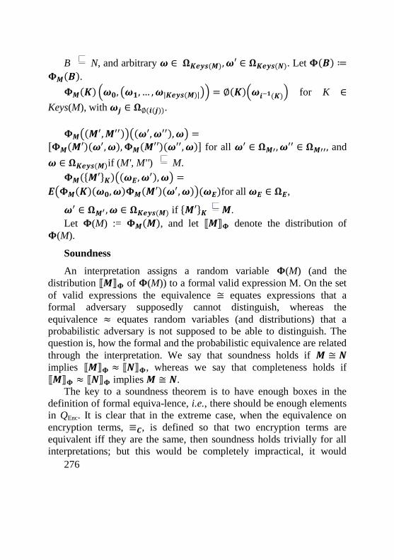
276

B N, and arbitrary 𝝎 ∈ 𝛀𝑲𝒆𝒚𝒔(𝑴), 𝝎′ ∈ 𝛀𝑲𝒆𝒚𝒔(𝑵). Let 𝚽(𝑩) ≔

𝚽𝑴(𝑩).

𝚽𝑴(𝑲) (𝝎𝟎, (𝝎𝟏, … ,𝝎|𝑲𝒆𝒚𝒔(𝑴)|)) = ∅(𝑲)(𝝎𝒊−𝟏(𝑲)) for K ∈

Keys(M), with 𝝎𝒋 ∈ 𝛀∅(𝒊(𝒋)).

𝚽𝑴((𝑴′,𝑴′′))((𝝎′, 𝝎′′),𝝎) =

[𝚽𝑴(𝑴′)(𝝎′, 𝝎),𝚽𝑴(𝑴′′)(𝝎

′′, 𝝎)] for all 𝝎′ ∈ 𝛀𝑴′, 𝝎′′ ∈ 𝛀𝑴′′, and

𝝎 ∈ 𝛀𝑲𝒆𝒚𝒔(𝑴)if (M', M'') M.

𝚽𝑴({𝑴′}𝑲)((𝝎𝑬, 𝝎′),𝝎) =

𝑬(𝚽𝑴(𝑲)(𝝎𝟎, 𝝎)𝚽𝑴(𝑴′)(𝝎′, 𝝎))(𝝎𝑬)for all 𝝎𝑬 ∈ 𝛀𝑬,

𝝎′ ∈ 𝛀𝑴′ , 𝝎 ∈ 𝛀𝑲𝒆𝒚𝒔(𝑴) if {𝑴′}𝑲 𝑴.

Let 𝚽(M) := 𝚽𝑴(𝑴), and let ⟦𝑴⟧𝚽 denote the distribution of

𝚽(M).

Soundness

An interpretation assigns a random variable 𝚽(M) (and the

distribution ⟦𝑴⟧𝚽 of 𝚽(M)) to a formal valid expression M. On the set

of valid expressions the equivalence ≅ equates expressions that a

formal adversary supposedly cannot distinguish, whereas the

equivalence ≈ equates random variables (and distributions) that a

probabilistic adversary is not supposed to be able to distinguish. The

question is, how the formal and the probabilistic equivalence are related

through the interpretation. We say that soundness holds if 𝑴 ≅ 𝑵

implies ⟦𝑴⟧𝚽 ≈ ⟦𝑵⟧𝚽, whereas we say that completeness holds if

⟦𝑴⟧𝚽 ≈ ⟦𝑵⟧𝚽 implies 𝑴 ≅ 𝑵.

The key to a soundness theorem is to have enough boxes in the

definition of formal equiva-lence, i.e., there should be enough elements

in QEnc. It is clear that in the extreme case, when the equivalence on

encryption terms, ≡𝑪, is defined so that two encryption terms are

equivalent iff they are the same, then soundness holds trivially for all

interpretations; but this would be completely impractical, it would

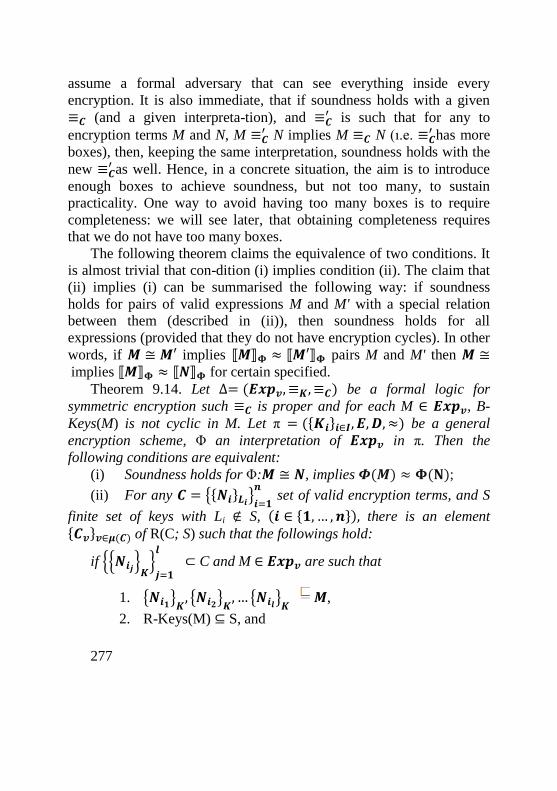
277

assume a formal adversary that can see everything inside every

encryption. It is also immediate, that if soundness holds with a given

≡𝑪 (and a given interpreta-tion), and ≡𝑪′ is such that for any to

encryption terms M and N, M ≡𝑪′ N implies M ≡𝑪 N (ı.e. ≡𝑪

′ has more

boxes), then, keeping the same interpretation, soundness holds with the

new ≡𝑪′ as well. Hence, in a concrete situation, the aim is to introduce

enough boxes to achieve soundness, but not too many, to sustain

practicality. One way to avoid having too many boxes is to require

completeness: we will see later, that obtaining completeness requires

that we do not have too many boxes.

The following theorem claims the equivalence of two conditions. It

is almost trivial that con-dition (i) implies condition (ii). The claim that

(ii) implies (i) can be summarised the following way: if soundness

holds for pairs of valid expressions M and M' with a special relation

between them (described in (ii)), then soundness holds for all

expressions (provided that they do not have encryption cycles). In other

words, if 𝑴 ≅ 𝑴′ implies ⟦𝑴⟧𝚽 ≈ ⟦𝑴′⟧𝚽 pairs M and M' then 𝑴 ≅ implies ⟦𝑴⟧𝚽 ≈ ⟦𝑵⟧𝚽 for certain specified.

Theorem 9.14. Let ∆= (𝑬𝒙𝒑𝒗, ≡𝑲, ≡𝑪) be a formal logic for

symmetric encryption such ≡𝑪 is proper and for each M ∈ 𝑬𝒙𝒑𝒗, B-

Keys(M) is not cyclic in M. Let π = ({𝑲𝒊}𝒊∈𝑰, 𝑬, 𝑫,≈) be a general

encryption scheme, Φ an interpretation of 𝑬𝒙𝒑𝒗 in π. Then the

following conditions are equivalent:

(i) Soundness holds for Φ:𝑴 ≅ 𝑵, implies 𝜱(𝑴) ≈ 𝚽(𝐍);

(ii) For any 𝑪 = {{𝑵𝒊}𝑳𝒊}𝒊=𝟏𝒏

set of valid encryption terms, and S

finite set of keys with Li ∉ S, (𝒊 ∈ {𝟏,… , 𝒏}), there is an element

{𝑪𝒗}𝒗∈𝝁(𝑪) of R(C; S) such that the followings hold:

if {{𝑵𝒊𝒋}𝑲}𝒋=𝟏

𝒍 ⊂ C and M ∈ 𝑬𝒙𝒑𝒗 are such that

1. {𝑵𝒊𝟏}𝑲, {𝑵𝒊𝟐}𝑲

, … {𝑵𝒊𝒍}𝑲 𝑴,

2. R-Keys(M) ⊆ S, and

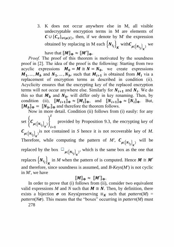
278

3. K does not occur anywhere else in M, all visible

undecryptable encryption terms in M are elements of

𝑪 ∪ {𝑪𝒗}𝒗∈𝝁(𝑪), then, if we denote by M' the expression

obtained by replacing in M each {𝑵𝒊𝒋}𝑲 with𝑪

𝝁({𝑵𝒊𝒋}𝑲) we

have that ⟦𝑴⟧𝚽 ≈ ⟦𝑴′⟧𝚽.

Proof. The proof of this theorem is motivated by the soundness

proof in [2]. The idea of the proof is the following: Starting from two

acyclic expressions 𝑴𝟎 = 𝑴 ≅ 𝑵 = 𝑵𝟎, we create expressions

𝑴𝟏, … ,𝑴𝒃 and 𝑵𝟏, … ,𝑵𝒃′ such that 𝑴𝒊+𝟏 is obtained from 𝑴𝒊 via a

replacement of encryption terms as described in condition (ii).

Acyclicity ensures that the encrypting key of the replaced encryption

terms will not occur anywhere else. Similarly for 𝑵𝒊+𝟏 and 𝑵𝒊. We do

this so that 𝑴𝒃 and 𝑵𝒃′ will differ only in key renaming. Then, by

condition (ii), ⟦𝑴𝒊+𝟏⟧𝚽 ≈ ⟦𝑴𝒊⟧𝚽, and ⟦𝑵𝒊+𝟏⟧𝚽 ≈ ⟦𝑵𝒊⟧𝚽. But,

⟦𝑴𝒃⟧𝚽 = ⟦𝑵𝒃′⟧𝚽 and therefore the theorem follows.

Now in more detail. Condition (ii) follows from (i) easily: for any

set {𝑪𝝁({𝑵𝒊𝒋}𝑲

)}𝒊=𝟏

𝒍

provided by Proposition 9.3, the encrypting key of

𝑪𝝁({𝑵𝒊𝒋}𝑲

)is not contained in S hence it is not recoverable key of M.

Therefore, while computing the pattern of M', 𝑪𝝁({𝑵𝒊𝒋}𝑲

) will be

replaced by the box 𝝁({𝑵𝒊𝒋}𝑲

), which is the same box as the one that

replaces {𝑵𝒊𝒋}𝑲 in M when the pattern of is computed. Hence 𝑴 ≅ 𝑴′

and therefore, since soundness is assumed, and B-Keys(M') is not cyclic

in M', we have

⟦𝑴⟧𝚽 ≈ ⟦𝑴′⟧𝚽.

In order to prove that (i) follows from (ii), consider two equivalent

valid expressions M and N such that 𝑴 ≅ 𝑵. Then, by definition, there

exists a bijection 𝝈 on Keys(preserving ≡𝑲 such that pattern(M) =

pattern(N𝝈). This means that the “boxes” occurring in pattern(M) must

279

oc-cur in pattern(N 𝝈) and vice-versa. Also, the subexpressions of

pattern(M) and of pattern(N 𝝈) outside the boxes must agree as well.

Hence,

𝑹−𝑲𝒆𝒚𝒔(𝑴) = 𝑹 − 𝑲𝒆𝒚𝒔(𝑵𝝈) = 𝑹 − 𝑲𝒆𝒚𝒔(𝑵)𝝈. Let L1, L2 ,...,Lb (Li ≠ Lj if i ≠ j) denote the keys in B-Keys(M), and

let L'1, L

'2,..., L

'b' (L'i ≠L'j if i ≠ j) denote the keys in B-Keys(N) 𝝈. B-

Keys(M) and B-Keys(N) (and therefore B-Keys(N 𝝈) as well) are not

cyclic by hypothesis, so without loss of generality, we can assume that

the Li’s and the L'i’s are numbered in such a way that Li encrypts Lj (and

L'i encrypts L'j) only if i < j (for a more detailed argument about this,

see [2]; intuitively this means that those keys in B-Keys(M) that are

deeper in M have a higher number).

Consider now the set of expressions that are subexpressions of M or

N and have the form {𝑴′}𝑳𝒊 𝒐𝒓 {𝑵′}𝑳′𝒊 , and also, the set S. Condition

(ii) then provides the set with elements of the form 𝑪𝝁({𝑴′}𝑳𝒊) and

𝑪𝝁({𝑵′}𝑳′𝒊).

Let M0 = M. Let M1 be the expression obtained from M0 by

replacing all subexpressions in M0 of the form {𝑴′}𝑳𝟏 by 𝑪𝝁({𝑴′}𝑳𝟏)

given by the assumption. Let then Mi, i ≥ 2, be the expression obtained

from 𝑴𝒊−𝟏 by replacing all subexpressions in 𝑴𝒊−𝟏 of the form {𝑴′}𝑳𝒊

by 𝑪𝝁({𝑴′}𝑳𝒊). We do this for all i ≤ b and it is easy to see that in Mb

replacing the subexpressions of the form 𝑪𝝁({𝑴′}𝑳𝒊) by 𝝁({𝑴′}𝑳𝒊)

for all

i, we arrive at pattern(M).

Note that in 𝑴𝒊−𝟏, Li can only occur as an encrypting key. The

reason for this is that if Li is a subexpression of M, then it has to be

encrypted with some non-recoverable key, otherwise Li would be

recoverable; moreover, it has to be encrypted with some key in B-

Keys(M) because a subexpression of M is either recoverable or ends up

in a box when we construct pattern(M). Now, the element in B-Keys(M)

that encrypts Li has to be an L j with j < i. But, all subexpres-sions in M

of the form fM 0 gLj were already replaced by 𝑪𝝁({𝑴′}𝑳𝒋)

when we

280

constructed Mj. According to the properties listed in proposition 2.13, Li

may only appear in 𝑪𝝁({𝑴′}𝑳𝒋) as the encrypting key, and then Li = Lj, a

contradiction. So Li cannot appear in Mi¡1 in any other place than an

encrypting key. Observe as well, that R-Keys(Mi) = R-Keys(M).

From assumption (ii), it follows then that ⟦𝑴𝒊−𝟏⟧𝚽 ≈ ⟦𝑴𝒊⟧𝚽, for

all i, 𝟏 ≤ 𝒊 ≤ 𝒃. Hence,

⟦𝐌⟧𝚽 = ⟦𝐌𝟎⟧𝚽 ≈ ⟦𝐌𝐛⟧𝚽 (2.3) Carrying out the same process for N𝝈 through (N𝝈)0, (N𝝈1, ...,

(N𝝈)b' we arrive at

⟦𝛔⟧𝚽 = ⟦(𝐍𝛔)𝟎⟧𝚽 ≈ ⟦(𝐍𝛔)𝐛′⟧𝚽 (2.4) Since we supposed that M ≅ N, that is, pattern(M) = pattern(N𝝈),

and therefore M b » pattern(M) and (N𝝈)b0 = pattern(N𝝈), we have

⟦𝐌𝐛⟧𝚽= ⟦(𝐍𝛔)𝐛′⟧𝚽 (2.5) Then, it is clearly true that

⟦𝐍⟧𝚽 ≈ ⟦𝐍𝛔⟧𝚽 (2.6) because permuting the keys in N does not have any effect in the

distributions. Putting together Equations (2.3), (2.4), (2.5) and (2.6) the

soundness result follows:

⟦𝐌⟧𝚽 ≈ ⟦𝐍⟧𝚽 Remark 9.3. The reason there is no similar general theorem for key-

cycles and KDM-like security is that this general soundness theorem

tells us in which conditions the several steps of the Abadi-Rogaway

hybrid argument can be carried out. One of the conditions is that by

doing one step of replacement, we must obtain equivalent

interpretations, provided that we have the appropriate security notion.

However, in our theorem using KDM security to solve the key-cycles

issue, there is only one step of replacement! All the replacements of

undecryptable terms is done at once. Therefore, in a general theorem

(without assuming a specific security level), the condition of the

theorem would have to be exactly what we would want to prove.

281

Example 9.12 (Type-1 Soundness). The soundness theorem that

was presented earlier for type-1 encryption schemes is a special case of

the theorem above. In this case Expv = Exp; the equivalence relation ≡𝑪

is proper; and the equivalence relation ≡𝑲 is trivial here, all keys are

equivalent. The elements 𝝁 ∈ QEnc are in one-to-one correspondence

with the possible length, so the patterns that we obtain this way are

essentially the same what we defined earlier, and the equivalence of

expressions will be ≅𝟏 that we also defined there. In order to see that

condition (ii) of the general soundness theorem is satisfied for type-1,

we will use the following equivalent definition of type-1 secure

encryption schemes: we can also say that an encryption-scheme is type-

1 secure if no PPT adversary A can distinguish the pair of oracles (E(k,

•, •, 0); E(k', •, •, 0)) and (E(k, •, •, 1); E(k, •, •, 1)) as k and k' are

independently generated, that is, for all PPT adversaries A:

𝐏𝐫[𝒌, 𝒌′ ← 𝑲(𝟏𝛈):𝑨𝑬(𝒌,•,•,𝟎),𝑬(𝒌′,•,•,𝟎)(𝟏𝛈) = 𝟏] −

𝐏𝐫 [𝒌 ← 𝑲(𝟏𝛈): 𝑨𝑬(𝒌,•,•,𝟏),𝑬(𝒌′,•,•,𝟏)(𝟏𝛈) = 𝟏] ≤ 𝒏𝒆𝒈(𝛈)

where the oracle 𝑬(𝒌,•,•, 𝟎), upon the submission of two messages

with equal lengths encrypts the first, and the oracle 𝑬(𝒌,•,•, 𝟏) encrypts

the second.

To show that condition (ii) of Theorem 9.14 holds, we first have to

choose for {𝑪𝒗}𝒗∈𝝁(𝑪) a given set 𝑪 = {{𝑵𝒊}𝑳𝒊}𝒊=𝟏𝒏 . We can choose any

family {𝑪𝒗}𝒗∈𝝁(𝑪) such that all the 𝑪𝒗 are encrypted with the same key,

let’s call it L0, that is not present in any of the {𝑵𝒊}𝑳𝒊 (neither in M).

This is possible, because, as it is easy to check,

𝒗𝒌𝒆𝒚 = 𝑲𝒆𝒚𝒔 𝐟𝐨𝐫 𝐚𝐥𝐥 𝒗 ∈ 𝑸𝑬𝒏𝒄. Then, let M be as in condition (ii).

We need to show that if {{𝑵𝒊𝒋}𝑳}𝒋=𝟏𝒍 ⊆ 𝑪 and if we denote by M'

the

expression obtained from M by replacing each {𝑵𝒊𝒋}𝑳 with 𝑪𝝁({𝑵𝒊𝒋}𝑳

),

then ⟦𝑴⟧𝚽 ≈ ⟦𝑴′⟧𝚽.

Suppose that ⟦𝑴⟧𝚽 ≈ ⟦𝑴′⟧𝚽, which means that there is an

adversary A that is able to distin-guish the two distributions, that is

𝐏𝐫 [𝒙 ← ⟦𝑴⟧𝚽𝛈: 𝑨(𝟏𝛈, 𝒙) = 𝟏] − 𝐏𝐫 [𝒙 ← ⟦𝑴′⟧𝚽𝛈: 𝑨(𝟏

𝛈, 𝒙) = 𝟏]

282

is a non-negligible function of η. Let us show that this contradicts

type-1 security. To this end, let us construct an adversary that can

distinguish between the two pair of oracles above. This adversary is the

following probabilistic algorithm that access to the oracles f and g:

algorithm B f,g

(𝟏𝛈; M)

for K ∈ Keys(M) \ {L, L0} do 𝝉(K) ← K(𝟏𝛈)

𝒚 ← 𝑪𝑶𝑵𝑽𝑬𝑹𝑻𝟐(𝑴) 𝒃 ← (𝟏𝛈, 𝒚)

return b

algorithm CONVERT2(N)

if N = K where K ∈ Keys then return 𝝉 (K)

if N = B where B ∈ Blocks then return B

if N = (M1; M2) then

𝒙 ← 𝑪𝑶𝑵𝑽𝑬𝑹𝑻𝟐(𝑴𝟏) y ← 𝑪𝑶𝑵𝑽𝑬𝑹𝑻𝟐(𝑴𝟐) return [x; y]

if N = {𝑴𝟏}𝑳 then

𝒙 ← 𝑪𝑶𝑵𝑽𝑬𝑹𝑻𝟐(𝑴𝟏) y ← 𝑪𝑶𝑵𝑽𝑬𝑹𝑻𝟐(𝑴𝒗) (where 𝑪𝝁({𝑴𝟏}𝑳) = {𝑴𝒗}𝑳𝟎)

𝒛 ← 𝒇(𝒙, 𝒚) return z

if N = {𝑴𝟏}𝑳𝟎 then

𝒙 ← 𝑪𝑶𝑵𝑽𝑬𝑹𝑻𝟐(𝑴𝟏) 𝒚 ← 𝒈(𝒙, 𝒙)

return y

if N = {𝑴𝟏}𝑲 (𝑲 ∉ {𝑳, 𝑳𝟎}) then

𝒙 ← 𝑪𝑶𝑵𝑽𝑬𝑹𝑻𝟐(𝑴𝟏) 𝒚 ← 𝑬(𝝉(𝑲), 𝒙)

return y

Note that the algorithm CONVERT2 does almost the same as the

algorithm CONVERT in Figure 9.1, except that while CONVERT

carries out all the necessary encryptions, CONVERT2 makes the

oracles carry out the encryptions for L and L0. Therefore, in the case,

283

when the pair of oracles (f; g) is (E(k, •, •, 0); E(k', •, •, 0)), then

CONVERT2(M) will be a random sample from ⟦𝑴⟧𝚽𝛈, whereas if the

pair of oracles used is (E(k, •, •, 1),E(k, •, •, 0)), then CONVERT2(M)

will be a random sample from ⟦𝑴′⟧𝚽𝛈. Thus,

𝐏𝐫[𝒌, 𝒌′ ← 𝑲(𝟏𝛈):𝑩𝑬(𝒌,•,•,𝟎),𝑬(𝒌′,•,•,𝟎)(𝟏𝛈,𝑴) = 𝟏] − 𝐏𝐫 [𝒙

← ⟦𝑴⟧𝚽𝛈: 𝑨(𝟏𝛈, 𝒙) = 𝟏]

and

𝐏𝐫[𝒌 ← 𝑲(𝟏𝛈): 𝑩𝑬(𝒌,•,•,𝟏),𝑬(𝒌,•,•,𝟏)(𝟏𝛈,𝑴) = 𝟏] − 𝐏𝐫 [𝒙

← ⟦𝑴′⟧𝚽𝛈: 𝑨(𝟏𝛈, 𝒙) = 𝟏]

But, according to our assumption, ⟦𝑴⟧𝚽 and ⟦𝑴′⟧𝚽 can be

distinguished, that is,

𝐏𝐫 [𝒙 ← ⟦𝑴⟧𝚽𝛈 ∶ 𝑨(𝟏𝛈, 𝒙) = 𝟏] − 𝐏𝐫 [𝒙 ← ⟦𝑴′⟧𝚽𝛈𝑨(𝟏

𝛈, 𝒙) = 𝟏]

is a non-negligible function of 𝛈 and so, there is an adversary B f,g

(𝟏𝛈, 𝒙) such that

𝐏r[𝒌, 𝒌′ ← 𝑲(𝟏𝛈): 𝑩𝑬(𝒌,•,•,𝟎),𝑬(𝒌′,•,•,𝟎)(𝟏𝛈,𝑴) = 𝟏] − 𝐏𝐫 [𝒌

← 𝑲(𝟏𝛈):𝑩𝑬(𝒌,•,•,𝟏),𝑬(𝒌,•,•,𝟏)(𝟏𝛈,𝑴) = 𝟏] is also a non-negligible function of 𝛈. This implies that our scheme

cannot be type-1 secure, which contradicts the assumption. Hence, we

cannot have ⟦𝑴⟧𝚽 ≈ ⟦𝑴′⟧𝚽. Hence, condition (ii) of the general

soundness theorem is satisfied, so soundness holds for the type-1 case.

Example 9.13 (Type-2 Soundness). The soundness theorem that

was presented earlier for type-2 encryption schemes is also a special

case of the theorem above. In this case ExpV = Exp; the equivalence

relation ≡𝑪 is is proper; and the equivalence relation ≡𝑲 is trivial here,

all keys are equivalent. The elements 𝝁 ∈ QEnc are in one-to-one

correspondence with the keys, so we can say QEnc ≡ Keys, and thus the

boxes are labelled with keys. In this case Φ gives an interpretation in

the computational setting. Then for a set 𝑪 = {{𝑵𝒊}𝑳𝒊}𝒊=𝟏𝒏 as in

condition (ii) of the theorem, we can take 𝑪𝑳𝒊 ≔ {𝟎}𝑳𝒊, and then

condition (ii) is satisfied, because the following proposition holds:

Proposition 9.4. Consider an expression M, and a key L ∈ Keys(M).

284

Suppose that for some expressions M1, M2, ..., Ml ∈ Exp,

{𝑴𝟏}𝑳, {𝑴𝟐}𝑳, … , {𝑴𝒍}𝑳 𝑴 , and assume also that L does not occur

anywhere else in M. Then, denoting by M' the expression that we get

from M by replacing each of {𝑴𝒊}𝑳 that are not contained in any of

𝑴𝒋(𝒋 ≠ 𝒊) by {𝟎}𝑳, ⟦𝑴⟧𝚽 ≈ ⟦𝑴′⟧𝚽 holds when the expressions are

interpreted with a type-2 encryption scheme.

Proof. We can assume, without loss of generality, that {𝑴𝒊}𝑳 is a

subexpression of {𝑴𝒋}𝑳 only if i < j. Suppose that ⟦𝑴⟧𝚽 ≈ ⟦𝑴′⟧𝚽,

which means that there is an adversary A that distinguishes the two

distributions, that is

𝐏𝐫 (𝒙 ← ⟦𝑴⟧𝚽𝛈 ∶ 𝑨(𝟏𝛈, 𝒙) = 𝟏) − 𝐏𝐫 (𝒙 ← ⟦𝑴′⟧𝚽𝛈 : 𝑨(𝟏

𝛈, 𝒙) = 𝟏)

is a non-negligible function of 𝛈. Let us show that this contradicts

type-2 security. To this end, let us construct an adversary that can

distinguish between the oracles E(k; •) and E(k; 0). This adversary is

the following probabilistic algorithm that access to the oracle f:

algorithm B f (𝟏𝛈; M)

for K ∈ 2 Keys(M) \ {L} do 𝝉(𝑲) ← K(𝟏𝛈)

𝒚 ← CONVERT2(M)

𝒃 ← A(𝟏𝛈; y) return b

algorithm CONVERT2(N)

if N = K where K ∈ Keys then return 𝝉 (K)

if N = B where B ∈ Blocks then

return B

if N = (N1; N2) then

𝒙 ←CONVERT2(N1) 𝒚 ←CONVERT2(N2) return [x; y]

if N = {𝑵𝟏}𝑳 then

𝒙 ← CONVERT2(N1) y 𝒚 ← f(x)

return y

if N = {𝑵𝟏}𝑲 (K ≠ L) then

𝒙 ← CONVERT2(N1)

𝒚 ← E(𝝉 (K); x) return y

285

Note that the algorithm CONVERT2 does almost the same as the

algorithm CONVERT in Figure 9.1, except that while CONVERT

carries out all necessary encryptions, CONVERT2 makes the oracles

carry out the encryptions for L. Therefore, in the case, when the oracle f

is E(k; • ), then CONVERT2(M) will be a random sample from ⟦𝑴⟧𝚽𝛈,

whereas if the oracle used is E(k; 0), then CONVERT2(M) will be a

random sample from ⟦𝑴′⟧𝚽𝛈. Thus,

𝐏𝐫[𝒌 ← 𝑲(𝟏𝛈) ∶ 𝑩𝑬(𝒌; • )(𝟏𝛈,𝑴) = 𝟏]

= 𝐏𝐫 [𝒙 ← ⟦𝑴⟧𝚽𝛈: 𝑨(𝟏𝛈, 𝒙) = 𝟏]

And

𝐏𝐫[𝒌 ← 𝑲(𝟏𝛈) ∶ 𝑩𝑬(𝒌; 𝟎)(𝟏𝛈,𝑴) = 𝟏]

= 𝐏𝐫 [𝒙 ← ⟦𝑴′⟧𝚽𝛈: 𝑨(𝟏𝛈, 𝒙) = 𝟏]

But, according to our assumption, ⟦𝑴⟧𝚽 and ⟦𝑴′⟧𝚽 can be

distinguished, that is,

𝐏𝐫 [𝒙 ← ⟦𝑴⟧𝚽𝛈 ∶ 𝑨(𝟏𝛈,𝑴) = 𝟏] − 𝐏𝐫 [𝒙 ← ⟦𝑴′⟧𝚽𝛈: 𝑨(𝟏

𝛈, 𝒙) = 𝟏]

is a non-negligible function of 𝛈 and so, there is an adversary B f

(𝟏𝛈, •) that can distinguish the oracles E(k, •) and E(k, 0), for randomly

generated keys k. This implies that our scheme cannot be type-2 secure,

which contradicts the assumption. Hence, we cannot have ⟦𝑴⟧𝚽 ≈⟦𝑴′⟧𝚽.

Hence, condition (ii) of the general soundness theorem is satisfied,

so soundness holds for the type-2 case.

Example 9.14 (Soundness for One-Time Pad). In order to see that

the formal treatment of Section sec:OTP is a special case of the general

formalism, take ≡𝑪 so that two encryption terms are equivalent, iff

(again) the encryption terms have the same encrypting key. The

equivalence of keys, ≡𝑲 is defined with the help of a length-function l

on the keys: two keys are equivalent iff they have the same length. The

boxes will again be indexed by the encrypting keys. Then for a set

𝑪 = {{𝑵𝒊}𝑳𝒊}𝒊=𝟏𝒏 as in condition (ii), take 𝑪𝑳𝒊 ≔ {𝟎𝒍(𝑳𝒊)−𝟑}𝑳𝒊 (where

𝟎𝒍(𝑳𝒊)−𝟑 means l(Li) - 3 many 0’s). It is not hard to check that within

286

this setting, condition (ii) of the soundness theorem is satisfied, which

is an immediate consequence of the following proposition:

Proposition 9.5. Consider a valid expression M ∈ ExpOTP, and a key

K0 ∈ Keys(M). Sup-pose that for some expression M0, {𝑴𝟎}𝑲𝟎 is a

subexpression of M, and assume also that K0 does not occur anywhere

else in M. Then, denoting by M' the expression that we get from M by

replacing {𝑴𝟎}𝑲𝟎 with {𝟎𝒍(𝑳𝒊)−𝟑}𝑲𝟎 (where 𝟎𝒍(𝑳𝒊)−𝟑 denotes as string

consisting of l(K0) - 3 many 0’s), the following is true when Φ is the

interpretation for OTP:

⟦𝐌⟧𝚽 = ⟦𝐌′⟧𝚽 (2.7) Proof. The basic properties of the OTP ensure that 𝚽({𝑴𝟎}𝑲𝟎) is

evenly distributed over the set of l(K0) long strings ending with 110, no

matter what M0 is. So the distribution of 𝚽({𝑴𝟎}𝑲𝟎) agrees with the

distribution of 𝚽({𝟎𝒍(𝑲𝟎)−𝟑}𝑲𝟎). Also, since K0 is assumed not to occur

anywhere else, 𝚽𝑴(K0) is independent of the interpretation of the rest

of the expression M, and therefore, 𝚽({𝑴𝟎}𝑲𝟎) and 𝚽({𝟎𝒍(𝑲𝟎)−𝟑}𝑲𝟎)

are both independent of the interpretation of the rest of the expression.

Hence, replacing 𝚽({𝑴𝟎}𝑲𝟎) with 𝚽({𝟎𝒍(𝑲𝟎)−𝟑}𝑲𝟎) will not effect the

distribution.

Parsing Process

Let us present the the chapter will be useful in the course of proving

the completeness results. The idea can be summarised as follows:

Given a sample element 𝒙 ← ⟦𝑴⟧𝚽, x is built from blocks and

randomly generated keys which are paired and encrypted. Some of the

keys that were used for encryption when x was built might be explicitly

contained in x, and in this case, using these keys, we can decrypt those

ciphers that were encrypted with these revealed keys. The problem is

though, that looking at x, it might not be possible to tell where blocks,

keys, ciphers and pairs are in the string of bits, since we did not assume

in general that we tag strings as we did for OTP. However, and we will

exploit this fact repeatedly in our proofs, if we know that x was

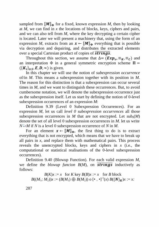
287

sampled from ⟦𝑴⟧𝚽 for a fixed, known expression M, then by looking

at M, we can find in x the locations of blocks, keys, ciphers and pairs,

and we can also tell from M, where the key decrypting a certain cipher

is located. Later we will present a machinery that, using the form of an

expression M, extracts from an 𝒙 ← ⟦𝑴⟧𝚽 everything that is possible

via decryption and depairing, and distributes the extracted elements

over a special Cartesian product of copies of 𝒔𝒕𝒓𝒊𝒏𝒈𝒔̅̅ ̅̅ ̅̅ ̅̅ ̅̅ ̅. Throughout this section, we assume that ∆= (𝑬𝒙𝒑𝒗, ≡𝑲, ≡𝑪) and

an interpretation Φ in a general symmetric encryption scheme 𝚷 =({𝑲𝒊}𝒊∈𝑰, 𝑬, 𝑫,≈) is given.

In this chapter we will use the notion of subexpression occurrence

of/in M. This means a subexpression together with its position in M.

The reason for this distinction is that a subexpression can occur several

times in M, and we want to distinguish these occurrences. But, to avoid

cumbersome notation, we will denote the subexpression occurrence just

as the subexpression itself. Let us start by defining the notion of 0-level

subexpression occurrences of an expression M:

Definition 9.39 (Level 0 Subexpression Occurrences). For an

expression M, let us call level 0 subexpression occurrences all those

subexpression occurrences in M that are not encrypted. Let sub0(M)

denote the set of all level 0 subexpression occurrences in M. let us write

N M if N is a level 0 subexpression occurrence of N in M.

For an element 𝒙 ← ⟦𝑴⟧𝚽, the first thing to do is to extract

everything that is not encrypted, which means that we have to break up

all pairs in x, and replace them with mathematical pairs. This process

reveals the unencrypted blocks, keys and ciphers in x (i.e., the

computational or statistical realisations of the 0-level subexpression

occurrences).

Definition 9.40 (Blowup Function). For each valid expression M,

we define the blowup funcion B(M), on 𝒔𝒕𝒓𝒊𝒏𝒈𝒔̅̅ ̅̅ ̅̅ ̅̅ ̅̅ ̅ inductively as

follows:

B(K)x := x for K key B(B)x := x for B block

B((M1; M2))x := (B(M1) ⊕ B(M2)) o [• , •]-1(x) B({𝑵}𝑲)x := x:

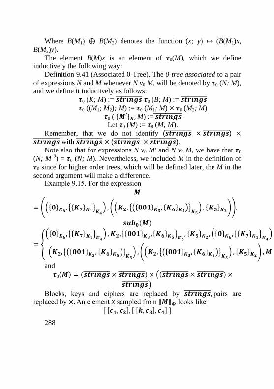
288

Where B(M1) ⊕ B(M2) denotes the function (x; y) ↦ (B(M1)x,

B(M2)y).

The element B(M)x is an element of 𝝉0(M), which we define

inductively the following way:

Definition 9.41 (Associated 0-Tree). The 0-tree associated to a pair

of expressions N and M whenever N v0 M, will be denoted by 𝝉0 (N; M),

and we define it inductively as follows:

𝝉0 (K; M) := 𝒔𝒕𝒓𝒊𝒏𝒈𝒔̅̅ ̅̅ ̅̅ ̅̅ ̅̅ ̅ 𝝉0 (B; M) := 𝒔𝒕𝒓𝒊𝒏𝒈𝒔̅̅ ̅̅ ̅̅ ̅̅ ̅̅ ̅ 𝝉0 ((M1; M2); M) := 𝝉0 (M1; M) × 𝝉0 (M2; M)

𝝉0 ( {𝑴′}𝑲, M) := 𝒔𝒕𝒓𝒊𝒏𝒈𝒔̅̅ ̅̅ ̅̅ ̅̅ ̅̅ ̅̅

Let 𝝉0 (M) := 𝝉0 (M; M).

Remember, that we do not identify (𝒔𝒕𝒓𝒊𝒏𝒈𝒔̅̅ ̅̅ ̅̅ ̅̅ ̅̅ ̅ × 𝒔𝒕𝒓𝒊𝒏𝒈𝒔̅̅ ̅̅ ̅̅ ̅̅ ̅̅ ̅) ×𝒔𝒕𝒓𝒊𝒏𝒈𝒔̅̅ ̅̅ ̅̅ ̅̅ ̅̅ ̅ with 𝒔𝒕𝒓𝒊𝒏𝒈𝒔̅̅ ̅̅ ̅̅ ̅̅ ̅̅ ̅ × (𝒔𝒕𝒓𝒊𝒏𝒈𝒔̅̅ ̅̅ ̅̅ ̅̅ ̅̅ ̅ × 𝒔𝒕𝒓𝒊𝒏𝒈𝒔̅̅ ̅̅ ̅̅ ̅̅ ̅̅ ̅).

Note also that for expressions N v0 M' and N v0 M, we have that 𝝉0

(N; M 0) = 𝝉0 (N; M). Nevertheless, we included M in the definition of

𝝉0 since for higher order trees, which will be defined later, the M in the

second argument will make a difference.

Example 9.15. For the expression

𝑴

= (({𝟎}𝑲𝟔 , {{𝑲𝟕}𝑲𝟏}𝑲𝟒) , ((𝑲𝟐, {({𝟎𝟎𝟏}𝑲𝟑 , {𝑲𝟔}𝑲𝟓)}𝑲𝟓

) , {𝑲𝟓}𝑲𝟐)),

𝒔𝒖𝒃𝟎(𝑴)

= {

({𝟎}𝑲𝟔 , {{𝑲𝟕}𝑲𝟏}𝑲𝟒) , 𝑲𝟐, {{𝟎𝟎𝟏}𝑲𝟑 , {𝑲𝟔}𝑲𝟓}𝑲𝟓

, {𝑲𝟓}𝑲𝟐 , ({𝟎}𝑲𝟔 , {{𝑲𝟕}𝑲𝟏}𝑲𝟒) ,

(𝑲𝟐, {({𝟎𝟎𝟏}𝑲𝟑 , {𝑲𝟔}𝑲𝟓)}𝑲𝟓) , ((𝑲𝟐, {({𝟎𝟎𝟏}𝑲𝟑 , {𝑲𝟔}𝑲𝟓)}𝑲𝟓

) , {𝑲𝟓}𝑲𝟐) ,𝑴}

and

𝝉0(𝑴) = (𝒔𝒕𝒓𝒊𝒏𝒈𝒔̅̅ ̅̅ ̅̅ ̅̅ ̅̅ ̅ × 𝒔𝒕𝒓𝒊𝒏𝒈𝒔̅̅ ̅̅ ̅̅ ̅̅ ̅̅ ̅) × ((𝒔𝒕𝒓𝒊𝒏𝒈𝒔̅̅ ̅̅ ̅̅ ̅̅ ̅̅ ̅ × 𝒔𝒕𝒓𝒊𝒏𝒈𝒔̅̅ ̅̅ ̅̅ ̅̅ ̅̅ ̅) ×

𝒔𝒕𝒓𝒊𝒏𝒈𝒔̅̅ ̅̅ ̅̅ ̅̅ ̅̅ ̅). Blocks, keys and ciphers are replaced by 𝒔𝒕𝒓𝒊𝒏𝒈𝒔̅̅ ̅̅ ̅̅ ̅̅ ̅̅ ̅, pairs are

replaced by ×. An element x sampled from ⟦𝑴⟧𝚽 looks like

[ [𝒄𝟏, 𝒄𝟐], [ [𝒌, 𝒄𝟑], 𝒄𝟒] ]

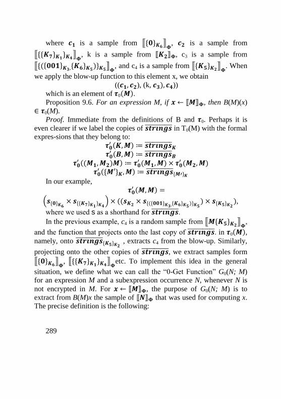
289

where 𝒄𝟏 is a sample from ⟦{𝟎}𝑲𝟔⟧𝚽, 𝒄𝟐 is a sample from

⟦{{𝑲𝟕}𝑲𝟏}𝑲𝟒⟧𝚽, k is a sample from ⟦𝑲𝟐⟧𝚽, c3 is a sample from

⟦{({𝟎𝟎𝟏}𝑲𝟑,{𝑲𝟔}𝑲𝟓)}𝑲𝟓⟧𝚽, and c4 is a sample from ⟦{𝑲𝟓}𝑲𝟐⟧𝚽

. When

we apply the blow-up function to this element x, we obtain

((𝒄𝟏, 𝒄𝟐), (k, 𝒄𝟑), 𝒄𝟒))

which is an element of 𝝉0(𝑴). Proposition 9.6. For an expression M, if 𝒙 ← ⟦𝑴⟧𝚽, then B(M)(x)

∈ 𝝉0(M).

Proof. Immediate from the definitions of B and 𝝉0. Perhaps it is

even clearer if we label the copies of 𝒔𝒕𝒓𝒊𝒏𝒈𝒔̅̅ ̅̅ ̅̅ ̅̅ ̅̅ ̅ in T0(M) with the formal

expres-sions that they belong to:

𝝉𝟎′ (𝑲,𝑴) ≔ 𝒔𝒕𝒓𝒊𝒏𝒈𝒔̅̅ ̅̅ ̅̅ ̅̅ ̅̅ ̅𝑲

𝝉𝟎′ (𝑩,𝑴) ≔ 𝒔𝒕𝒓𝒊𝒏𝒈𝒔̅̅ ̅̅ ̅̅ ̅̅ ̅̅ ̅𝑩

𝝉𝟎′ ((𝑴𝟏,𝑴𝟐)𝑴) ≔ 𝝉𝟎

′ (𝑴𝟏,𝑴) × 𝝉𝟎′ (𝑴𝟐,𝑴)

𝝉𝟎′ ({𝑴′}𝑲,𝑴) ≔ 𝒔𝒕𝒓𝒊𝒏𝒈𝒔̅̅ ̅̅ ̅̅ ̅̅ ̅̅ ̅{𝑴′}𝑲

In our example,

𝝉𝟎′ (𝑴,𝑴) =

(𝒔{𝟎}𝑲𝟔× 𝒔{{𝑲𝟕}𝑲𝟏}𝑲𝟒

) × ((𝒔𝑲𝟐 × 𝒔{({𝟎𝟎𝟏}𝑲𝟑,{𝑲𝟔}𝑲𝟓)}𝑲𝟓) × 𝒔{𝑲𝟓}𝑲𝟐

),

where we used s as a shorthand for 𝒔𝒕𝒓𝒊𝒏𝒈𝒔̅̅ ̅̅ ̅̅ ̅̅ ̅̅ ̅.

In the previous example, c4 is a random sample from ⟦𝑴{𝑲𝟓}𝑲𝟐⟧𝚽,

and the function that projects onto the last copy of 𝒔𝒕𝒓𝒊𝒏𝒈𝒔̅̅ ̅̅ ̅̅ ̅̅ ̅̅ ̅. in 𝝉0(𝑴), namely, onto 𝒔𝒕𝒓𝒊𝒏𝒈𝒔̅̅ ̅̅ ̅̅ ̅̅ ̅̅ ̅{𝑲𝟓}𝑲𝟐

, extracts c4 from the blow-up. Similarly,

projecting onto the other copies of 𝒔𝒕𝒓𝒊𝒏𝒈𝒔̅̅ ̅̅ ̅̅ ̅̅ ̅̅ ̅, we extract samples form

⟦{𝟎}𝑲𝟔⟧𝚽, ⟦{{𝑲𝟕}𝑲𝟏}𝑲𝟒⟧𝚽

etc. To implement this idea in the general

situation, we define what we can call the “0-Get Function” G0(N; M)

for an expression M and a subexpression occurrence N, whenever N is

not encrypted in M. For 𝒙 ← ⟦𝑴⟧𝚽, the purpose of G0(N; M) is to

extract from B(M)x the sample of ⟦𝑵⟧𝚽 that was used for computing x.

The precise definition is the following:

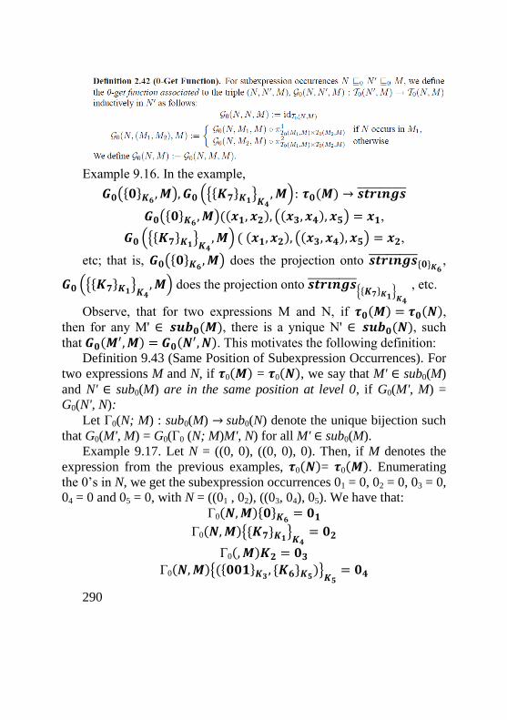
290

Example 9.16. In the example,

𝑮𝟎({𝟎}𝑲𝟔 ,𝑴), 𝑮𝟎 ({{𝑲𝟕}𝑲𝟏}𝑲𝟒,𝑴): 𝝉𝟎(𝑴) → 𝒔𝒕𝒓𝒊𝒏𝒈𝒔̅̅ ̅̅ ̅̅ ̅̅ ̅̅ ̅

𝑮𝟎({𝟎}𝑲𝟔 ,𝑴)((𝒙𝟏, 𝒙𝟐), ((𝒙𝟑, 𝒙𝟒), 𝒙𝟓) = 𝒙𝟏,

𝑮𝟎 ({{𝑲𝟕}𝑲𝟏}𝑲𝟒,𝑴) ( (𝒙𝟏, 𝒙𝟐), ((𝒙𝟑, 𝒙𝟒), 𝒙𝟓) = 𝒙𝟐,

etc; that is, 𝑮𝟎({𝟎}𝑲𝟔 ,𝑴) does the projection onto 𝒔𝒕𝒓𝒊𝒏𝒈𝒔̅̅ ̅̅ ̅̅ ̅̅ ̅̅ ̅{𝟎}𝑲𝟔,

𝑮𝟎 ({{𝑲𝟕}𝑲𝟏}𝑲𝟒,𝑴) does the projection onto 𝒔𝒕𝒓𝒊𝒏𝒈𝒔̅̅ ̅̅ ̅̅ ̅̅ ̅̅ ̅

{{𝑲𝟕}𝑲𝟏}𝑲𝟒

, etc.

Observe, that for two expressions M and N, if 𝝉𝟎(𝑴) = 𝝉𝟎(𝑵), then for any M' ∈ 𝒔𝒖𝒃𝟎(𝑴), there is a ynique N' ∈ 𝒔𝒖𝒃𝟎(𝑵), such

that 𝑮𝟎(𝑴′,𝑴) = 𝑮𝟎(𝑵

′, 𝑵). This motivates the following definition:

Definition 9.43 (Same Position of Subexpression Occurrences). For

two expressions M and N, if 𝝉0(𝑴) = 𝝉0(𝑵), we say that M' ∈ sub0(M)

and N' ∈ sub0(M) are in the same position at level 0, if G0(M', M) =

G0(N', N):

Let Г0(N; M) : sub0(M) → sub0(N) denote the unique bijection such

that G0(M', M) = G0(Г0 (N; M)M', N) for all M' ∈ sub0(M).

Example 9.17. Let N = ((0, 0), ((0, 0), 0). Then, if M denotes the

expression from the previous examples, 𝝉0(𝑵)= 𝝉0(𝑴). Enumerating

the 0’s in N, we get the subexpression occurrences 01 = 0, 02 = 0, 03 = 0,

04 = 0 and 05 = 0, with N = ((01 , 02), ((03, 04), 05). We have that:

Г0(𝑵,𝑴){𝟎}𝑲𝟔 = 𝟎𝟏

Г0(𝑵,𝑴){{𝑲𝟕}𝑲𝟏}𝑲𝟒= 𝟎𝟐

Г0(,𝑴)𝑲𝟐 = 𝟎𝟑

Г0(𝑵,𝑴){({𝟎𝟎𝟏}𝑲𝟑 , {𝑲𝟔}𝑲𝟓)}𝑲𝟓= 𝟎𝟒

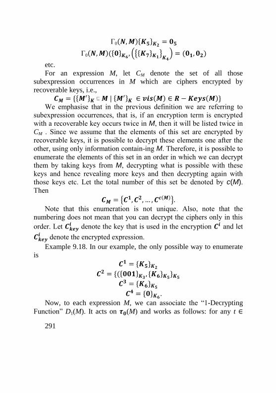
291

Г0(𝑵,𝑴){𝑲𝟓}𝑲𝟐 = 𝟎𝟓

Г0(𝑵,𝑴)({𝟎}𝑲𝟔 , ({{𝑲𝟕}𝑲𝟏}𝑲𝟒) = (𝟎𝟏, 𝟎𝟐)

etc.

For an expression M, let CM denote the set of all those

subexpression occurrences in M which are ciphers encrypted by

recoverable keys, i.e.,

𝑪𝑴 = {{𝑴′}𝑲 𝑴 | {𝑴′}𝑲 ∈ 𝒗𝒊𝒔(𝑴) ∈ 𝑹 − 𝑲𝒆𝒚𝒔(𝑴)}

We emphasise that in the previous definition we are referring to

subexpression occurrences, that is, if an encryption term is encrypted

with a recoverable key occurs twice in M, then it will be listed twice in

CM . Since we assume that the elements of this set are encrypted by

recoverable keys, it is possible to decrypt these elements one after the

other, using only information contain-ing M. Therefore, it is possible to

enumerate the elements of this set in an order in which we can decrypt

them by taking keys from M, decrypting what is possible with these

keys and hence revealing more keys and then decrypting again with

those keys etc. Let the total number of this set be denoted by c(M). Then

𝑪𝑴 = {𝑪𝟏, 𝑪𝟐, … , 𝑪𝒄(𝑴)}.

Note that this enumeration is not unique. Also, note that the

numbering does not mean that you can decrypt the ciphers only in this

order. Let 𝑪𝒌𝒆𝒚𝒊 denote the key that is used in the encryption 𝑪𝒊 and let

𝑪𝒌𝒆𝒚𝒊 denote the encrypted expression.

Example 9.18. In our example, the only possible way to enumerate

is

𝑪𝟏 = {𝑲𝟓}𝑲𝟐

𝑪𝟐 = {({𝟎𝟎𝟏}𝑲𝟑 , {𝑲𝟔}𝑲𝟓}𝑲𝟓

𝑪𝟑 = {𝑲𝟔}𝑲𝟓

𝑪𝟒 = {𝟎}𝑲𝟔.

Now, to each expression M, we can associate the “1-Decrypting

Function” D1(M). It acts on 𝝉𝟎(M) and works as follows: for any t ∈

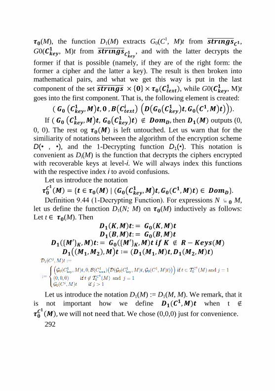
292

𝝉𝟎(M), the function D1(M) extracts G0(C1, M)t from 𝒔𝒕𝒓𝒊𝒏𝒈𝒔̅̅ ̅̅ ̅̅ ̅̅ ̅̅ ̅

𝑪𝟏,

G0(𝑪𝒌𝒆𝒚𝟏 , M)t from 𝒔𝒕𝒓𝒊𝒏𝒈𝒔̅̅ ̅̅ ̅̅ ̅̅ ̅̅ ̅

𝑪𝒌𝒆𝒚𝟏 , and with the latter decrypts the

former if that is possible (namely, if they are of the right form: the

former a cipher and the latter a key). The result is then broken into

mathematical pairs, and what we get this way is put in the last

component of the set 𝒔𝒕𝒓𝒊𝒏𝒈𝒔̅̅ ̅̅ ̅̅ ̅̅ ̅̅ ̅ × {𝟎} × 𝝉𝟎(𝑪𝒕𝒆𝒙𝒕𝟏 ), while G0(𝑪𝒌𝒆𝒚

𝟏 , M)t

goes into the first component. That is, the following element is created:

( 𝑮𝟎 (𝑪𝒌𝒆𝒚𝟏 ,𝑴)𝒕, 𝟎 , 𝑩(𝑪𝒕𝒆𝒙𝒕

𝒊 ) (𝑫(𝑮𝟎(𝑪𝒌𝒆𝒚𝟏 )𝒕, 𝑮𝟎(𝑪

𝟏,𝑴)𝒕))).

If ( 𝑮𝟎 (𝑪𝒌𝒆𝒚𝟏 ,𝑴)𝒕, 𝑮𝟎(𝑪𝒌𝒆𝒚

𝟏 )𝒕) ∉ 𝑫𝒐𝒎𝑫, then 𝑫𝟏(𝑴) outputs (0,

0, 0). The rest og 𝝉𝟎(𝑴) is left untouched. Let us warn that for the

similiarity of notations between the algorithm of the encryption scheme

D(• , •), and the 1-Decrypting function D1(•). This notation is

convenient as Di(M) is the function that decrypts the ciphers encrypted

with recoverable keys at level-i. We will always index this functions

with the respective index i to avoid confusions.

Let us introduce the notation

𝝉𝟎𝑪𝟏(𝑴) = {𝒕 ∈ 𝝉𝟎(𝑴) | (𝑮𝟎(𝑪𝒌𝒆𝒚

𝟏 ,𝑴)𝒕, 𝑮𝟎(𝑪𝟏,𝑴)𝒕) ∈ 𝑫𝒐𝒎𝑫}.

Definition 9.44 (1-Decrypting Function). For expressions N 𝟎 M,

let us define the function D1(N; M) on 𝝉𝟎(M) inductively as follows:

Let t ∈ 𝝉𝟎(M). Then

𝑫𝟏(𝑲,𝑴)𝒕:= 𝑮𝟎(𝑲,𝑴)𝒕 𝑫𝟏(𝑩,𝑴)𝒕:= 𝑮𝟎(𝑩,𝑴)𝒕

𝑫𝟏({𝑴′}𝑲,𝑴)𝒕:= 𝑮𝟎({𝑴′}𝑲,𝑴)𝒕 𝒊𝒇 𝑲 ∉ 𝑹 − 𝑲𝒆𝒚𝒔(𝑴) 𝑫𝟏((𝑴𝟏,𝑴𝟐),𝑴)𝒕 ∶= (𝑫𝟏(𝑴𝟏,𝑴)𝒕,𝑫𝟏(𝑴𝟐,𝑴)𝒕)

Let us introduce the notation D1(M) := D1(M, M). We remark, that it

is not important how we define 𝑫𝟏(𝑪𝟏,𝑴)𝒕 when t ∉

𝝉𝟎𝑪𝟏(𝑴),we will not need that. We chose (0,0,0) just for convenience.

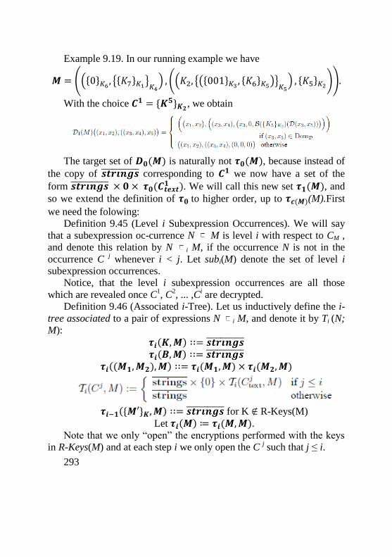
293

Example 9.19. In our running example we have

𝑴 = (({0}𝐾6 , {{𝐾7}𝐾1}𝐾4) , ((𝐾2, {({001}𝐾3 , {𝐾6}𝐾5)}𝐾5

) , {𝐾5}𝐾2)).

With the choice 𝑪𝟏 = {𝑲𝟓}𝑲𝟐, we obtain

The target set of 𝑫𝟎(𝑴) is naturally not 𝝉𝟎(𝑴), because instead of

the copy of 𝒔𝒕𝒓𝒊𝒏𝒈𝒔̅̅ ̅̅ ̅̅ ̅̅ ̅̅ ̅ corresponding to 𝑪𝟏 we now have a set of the

form 𝒔𝒕𝒓𝒊𝒏𝒈𝒔̅̅ ̅̅ ̅̅ ̅̅ ̅̅ ̅ × 𝟎 × 𝝉𝟎(𝑪𝒕𝒆𝒙𝒕𝟏 ). We will call this new set 𝝉𝟏(𝑴), and

so we extend the definition of 𝝉𝟎 to higher order, up to 𝝉𝒄(𝑴)(M).First

we need the folowing:

Definition 9.45 (Level i Subexpression Occurrences). We will say

that a subexpression oc-currence N M is level i with respect to CM ,

and denote this relation by N i M, if the occurrence N is not in the

occurrence C j whenever i < j. Let subi(M) denote the set of level i

subexpression occurrences.

Notice, that the level i subexpression occurrences are all those

which are revealed once C1, C

2, ... ,C

i are decrypted.

Definition 9.46 (Associated i-Tree). Let us inductively define the i-

tree associated to a pair of expressions N i M, and denote it by Ti (N;

M):

𝝉𝒊(𝑲,𝑴) ∷= 𝒔𝒕𝒓𝒊𝒏𝒈𝒔̅̅ ̅̅ ̅̅ ̅̅ ̅̅ ̅ 𝝉𝒊(𝑩,𝑴) ∷= 𝒔𝒕𝒓𝒊𝒏𝒈𝒔̅̅ ̅̅ ̅̅ ̅̅ ̅̅ ̅

𝝉𝒊((𝑴𝟏,𝑴𝟐),𝑴) ∷= 𝝉𝒊(𝑴𝟏,𝑴) × 𝝉𝒊(𝑴𝟐,𝑴)

𝝉𝒊−𝟏({𝑴′}𝑲,𝑴) ∷= 𝒔𝒕𝒓𝒊𝒏𝒈𝒔̅̅ ̅̅ ̅̅ ̅̅ ̅̅ ̅ for K ∉ R-Keys(M)

Let 𝝉𝒊(𝑴) ≔ 𝝉𝒊(𝑴,𝑴). Note that we only “open” the encryptions performed with the keys

in R-Keys(M) and at each step i we only open the C j such that j ≤ i.

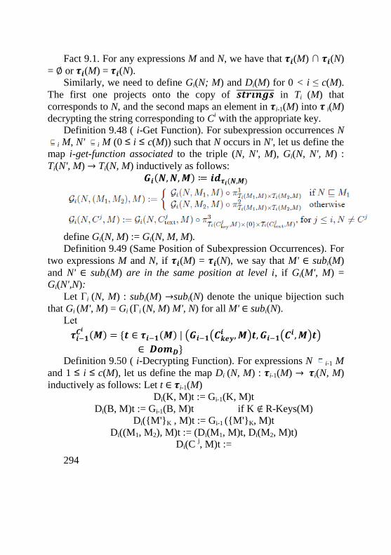
294

Fact 9.1. For any expressions M and N, we have that 𝝉𝒊(M) ∩ 𝝉𝒊(N)

= ∅ or 𝝉𝒊(M) = 𝝉𝒊(N).

Similarly, we need to define Gi(N; M) and Di(M) for 0 < i ≤ c(M).

The first one projects onto the copy of 𝒔𝒕𝒓𝒊𝒏𝒈𝒔̅̅ ̅̅ ̅̅ ̅̅ ̅̅ ̅ in Ti (M) that

corresponds to N, and the second maps an element in 𝝉i-1(M) into 𝝉 i(M)

decrypting the string corresponding to Ci with the appropriate key.

Definition 9.48 ( i-Get Function). For subexpression occurrences N

i M, N' i M (0 ≤ i ≤ c(M)) such that N occurs in N', let us define the

map i-get-function associated to the triple (N, N', M), Gi(N, N', M) :

Ti(N', M) → Ti(N, M) inductively as follows:

𝑮𝒊(𝑵,𝑵,𝑴) ≔ 𝒊𝒅𝝉𝒊(𝑵,𝑴)

define Gi(N, M) := Gi(N, M, M).

Definition 9.49 (Same Position of Subexpression Occurrences). For

two expressions M and N, if 𝝉𝒊(M) = 𝝉𝒊(N), we say that M' ∈ subi(M)

and N' ∈ subi(M) are in the same position at level i, if Gi(M', M) =

Gi(N',N):

Let Гi (N, M) : subi(M) →subi(N) denote the unique bijection such

that Gi (M', M) = Gi (Гi (N, M) M', N) for all M' ∈ subi(N).

Let

𝝉𝒊−𝟏𝑪𝒊 (𝑴) = {𝒕 ∈ 𝝉𝒊−𝟏(𝑴) | (𝑮𝒊−𝟏(𝑪𝒌𝒆𝒚

𝒊 ,𝑴)𝒕, 𝑮𝒊−𝟏(𝑪𝒊,𝑴)𝒕)

∈ 𝑫𝒐𝒎𝑫} Definition 9.50 ( i-Decrypting Function). For expressions N i-1 M

and 1 ≤ i ≤ c(M), let us define the map Di (N, M) : 𝝉i-1(M) → 𝝉i(N, M)

inductively as follows: Let t ∈ 𝝉i-1(M)

Di(K, M)t := Gi-1(K, M)t

Di(B, M)t := Gi-1(B, M)t if K ∉ R-Keys(M)

Di({M'}K , M)t := Gi-1 ({M'}K, M)t

Di((M1, M2), M)t := (Di(M1, M)t, Di(M2, M)t)

Di(C j, M)t :=

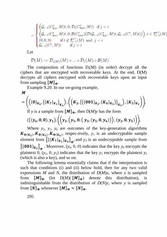
295

Let

The composition of functions Di(M) (in order) decrypt all the

ciphers that are encrypted with recoverable keys. At the end, D(M)

decrypts all ciphers encrypted with recoverable keys upon an input

from sampling ⟦𝑴⟧𝚽.

Example 9.20. In our on-going example,

𝑴

= (({𝟎}𝑲𝟔 , {{𝑲𝟕}𝑲𝟏}𝑲𝟒) , ((𝑲𝟐, {({𝟎𝟎𝟏}𝑲𝟑 , {𝑲𝟔}𝑲𝟓)}𝑲𝟓

) , {𝑲𝟓}𝑲𝟐)),

If y is a sample from ⟦𝑴⟧𝚽, then D(M)y has the form

(((𝒚𝟔, 𝟎, 𝟎), 𝒚𝟏), ((𝒚𝟐, (𝒚𝟓, 𝟎, ( 𝒚𝟑, (𝒚𝟓, 𝟎, 𝒚𝟔))) , (𝒚𝟐, 𝟎, 𝒚𝟓))),

Where y2, y5, y6 are outcomes of the key-generation algorithms

𝑲𝚽(𝐊𝟐), 𝑲𝚽(𝐊𝟓), 𝑲𝚽(𝐊𝟔), respec-tively, y1 is an undecryptable sample

element from ⟦{{𝑲𝟕}𝑲𝟏}𝑲𝟒⟧𝚽, and y3 is an undecryptable sample from

⟦{𝟎𝟎𝟏}𝐊𝟑⟧𝚽 . Moreover, (y6, 0, 0) indicates that the key y6 encrypts the

plaintext 0, (y2, 0, y5) indicates that the key y2 encrypts the plaintext y5

(which is also a key), and so on.

The following lemma essentially claims that if the interpretation is

such that conditions (i) and (ii) below hold, then for any two valid

expressions M and N, the distribution of D(M)x, where x is sampled

from ⟦𝑴⟧𝚽 (let D(M)( ⟦𝑴⟧𝚽) denote this distribution), is

indistinguishable from the distribution of D(N)y, where y is sampled

from ⟦𝑵⟧𝚽 whenever ⟦𝑴⟧𝚽 ≈ ⟦𝑵⟧𝚽.

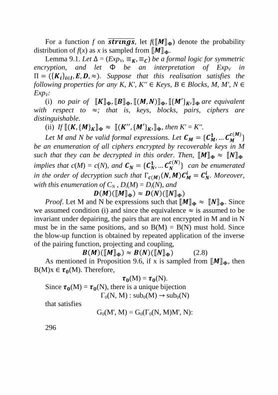
296

For a function f on 𝒔𝒕𝒓𝒊𝒏𝒈𝒔̅̅ ̅̅ ̅̅ ̅̅ ̅̅ ̅, let f(⟦𝑴⟧𝚽) denote the probability

distribution of f(x) as x is sampled from ⟦𝑴⟧𝚽.

Lemma 9.1. Let ∆ = (ExpV, ≡𝑲, ≡𝑪) be a formal logic for symmetric

encryption, and let Φ be an interpretation of ExpV in

П = ({𝑲𝒊}𝒊∈𝑰, 𝑬, 𝑫,≈). Suppose that this realisation satisfies the

following properties for any K, K', K'' ∈ Keys, B ∈ Blocks, M, M', N ∈

ExpV:

(i) no pair of ⟦𝑲⟧𝚽, ⟦𝑩⟧𝚽, ⟦(𝑴,𝑵)⟧𝚽, ⟦{𝑴′}𝑲′⟧𝚽 are equivalent

with respect to ≈; that is, keys, blocks, pairs, ciphers are

distinguishable.

(ii) If ⟦(𝑲, {𝑴}𝑲⟧𝚽 ≈ ⟦(𝑲′′, {𝑴′}𝑲′⟧𝚽, then K' = K''.

Let M and N be valid formal expressions. Let 𝑪𝑴 = {𝑪𝑴𝟏 , … 𝑪𝑴

𝒄(𝑴)}

be an enumeration of all ciphers encrypted by recoverable keys in M

such that they can be decrypted in this order. Then, ⟦𝑴⟧𝚽 ≈ ⟦𝑵⟧𝚽

implies that c(M) = c(N), and 𝑪𝑵 = {𝑪𝑵𝟏 , …𝑪𝑵

𝒄(𝑵)} can be enumerated

in the order of decryption such that Г𝒄(𝑴)(𝑵,𝑴)𝑪𝑴𝒊 = 𝑪𝑵

𝒊 . Moreover,

with this enumeration of CN , Di(M) = Di(N), and

𝑫(𝑴)(⟦𝑴⟧𝚽) ≈ 𝑫(𝑵)(⟦𝑵⟧𝚽) Proof. Let M and N be expressions such that ⟦𝑴⟧𝚽 ≈ ⟦𝑵⟧𝚽. Since

we assumed condition (i) and since the equivalence ≈ is assumed to be

invariant under depairing, the pairs that are not encrypted in M and in N

must be in the same positions, and so B(M) = B(N) must hold. Since

the blow-up function is obtained by repeated application of the inverse

of the pairing function, projecting and coupling,

𝑩(𝑴)(⟦𝑴⟧𝚽) ≈ 𝑩(𝑵)(⟦𝑵⟧𝚽) (2.8)

As mentioned in Proposition 9.6, if x is sampled from ⟦𝑴⟧𝚽, then

B(M)x ∈ 𝝉𝟎(M). Therefore,

𝝉𝟎(M) = 𝝉𝟎(N).

Since 𝝉𝟎(M) = 𝝉𝟎(N), there is a unique bijection

Г0(N, M) : sub0(M) → sub0(N)

that satisfies

G0(M', M) = G0(Г0(N, M)M', N):

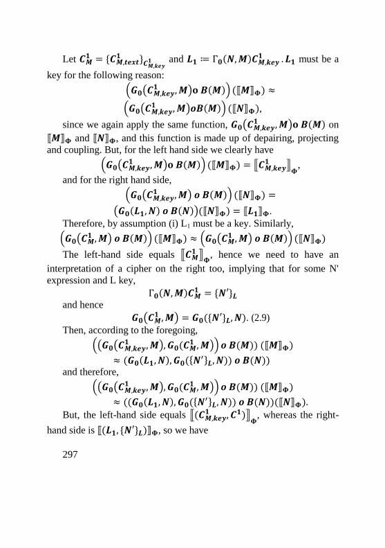
297

Let 𝑪𝑴𝟏 = {𝑪𝑴,𝒕𝒆𝒙𝒕

𝟏 }𝑪𝑴,𝒌𝒆𝒚𝟏 and 𝑳𝟏 ≔ Г𝟎(𝑵,𝑴)𝑪𝑴,𝒌𝒆𝒚

𝟏 . 𝑳𝟏 must be a

key for the following reason:

(𝑮𝟎(𝑪𝑴,𝒌𝒆𝒚𝟏 ,𝑴)𝐨 𝑩(𝑴)) (⟦𝑴⟧𝚽) ≈

(𝑮𝟎(𝑪𝑴,𝒌𝒆𝒚𝟏 ,𝑴)𝒐𝑩(𝑴)) (⟦𝑵⟧𝚽),

since we again apply the same function, 𝑮𝟎(𝑪𝑴,𝒌𝒆𝒚𝟏 ,𝑴)𝐨 𝑩(𝑴) on

⟦𝑴⟧𝚽 and ⟦𝑵⟧𝚽, and this function is made up of depairing, projecting

and coupling. But, for the left hand side we clearly have

(𝑮𝟎(𝑪𝑴,𝒌𝒆𝒚𝟏 ,𝑴)𝐨 𝑩(𝑴)) (⟦𝑴⟧𝚽) = ⟦𝑪𝑴,𝒌𝒆𝒚

𝟏 ⟧𝚽

,

and for the right hand side,

(𝑮𝟎(𝑪𝑴,𝒌𝒆𝒚𝟏 ,𝑴) 𝒐 𝑩(𝑴)) (⟦𝑵⟧𝚽) =

(𝑮𝟎(𝑳𝟏, 𝑵) 𝒐 𝑩(𝑵))(⟦𝑵⟧𝚽) = ⟦𝑳𝟏⟧𝚽.

Therefore, by assumption (i) L1 must be a key. Similarly,

(𝑮𝟎(𝑪𝑴𝟏 ,𝑴) 𝒐 𝑩(𝑴)) (⟦𝑴⟧𝚽) ≈ (𝑮𝟎(𝑪𝑴

𝟏 ,𝑴) 𝒐 𝑩(𝑴)) (⟦𝑵⟧𝚽)

The left-hand side equals ⟦𝑪𝑴𝟏 ⟧

𝚽, hence we need to have an

interpretation of a cipher on the right too, implying that for some N'

expression and L key,

Г𝟎(𝑵,𝑴)𝑪𝑴𝟏 = {𝑵′}𝑳

and hence

𝑮𝟎(𝑪𝑴𝟏 ,𝑴) = 𝑮𝟎({𝑵′}𝑳, 𝑵). (2.9)

Then, according to the foregoing,

((𝑮𝟎(𝑪𝑴,𝒌𝒆𝒚𝟏 ,𝑴), 𝑮𝟎(𝑪𝑴

𝟏 ,𝑴)) 𝒐 𝑩(𝑴)) (⟦𝑴⟧𝚽)

≈ (𝑮𝟎(𝑳𝟏, 𝑵), 𝑮𝟎({𝑵′}𝑳, 𝑵)) 𝒐 𝑩(𝑵))

and therefore,

((𝑮𝟎(𝑪𝑴,𝒌𝒆𝒚𝟏 ,𝑴), 𝑮𝟎(𝑪𝑴

𝟏 ,𝑴)) 𝒐 𝑩(𝑴)) (⟦𝑴⟧𝚽)

≈ ((𝑮𝟎(𝑳𝟏, 𝑵), 𝑮𝟎({𝑵′}𝑳, 𝑵)) 𝒐 𝑩(𝑵))(⟦𝑵⟧𝚽).

But, the left-hand side equals ⟦(𝑪𝑴,𝒌𝒆𝒚𝟏 , 𝑪𝟏)⟧

𝚽, whereas the right-

hand side is ⟦(𝑳𝟏, {𝑵′}𝑳)⟧𝚽, so we have

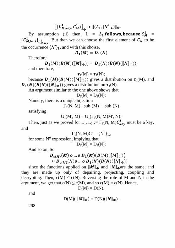
298

⟦(𝑪𝑴,𝒌𝒆𝒚𝟏 , 𝑪𝑴

𝟏 )⟧𝚽≈ ⟦(𝑳𝟏, {𝑵′}𝑳)⟧𝚽.

By assumption (ii) then, L = 𝑳𝟏 𝐟𝐨𝐥𝐥𝐨𝐰𝐬, 𝐛𝐞𝐜𝐚𝐮𝐬𝐞 𝑪𝑴𝟏 =

{𝑪𝑴,𝒕𝒆𝒙𝒕𝟏 }𝑪𝑴,𝒌𝒆𝒚

𝟏 . But then we can choose the first element of 𝑪𝑵 to be

the occurrence {𝑵′}𝑳, and with this choise,

𝑫𝟏(𝑴) = 𝑫𝟏(𝑵) Therefore

𝑫𝟏(𝑴)(𝑩(𝑴)(⟦𝑴⟧𝚽)) ≈ 𝑫𝟏(𝑵)(𝑩(𝑵)(⟦𝑵⟧𝚽)), and therefore,

𝝉1(M) = 𝝉1(N);

because 𝑫𝟏(𝑴)(𝑩(𝑴)(⟦𝑴⟧𝚽)) gives a distribution on 𝝉1(M), and

𝑫𝟏(𝑵)(𝑩(𝑵)(⟦𝑵⟧𝚽)) gives a distribution on 𝝉1(N).

An argument similar to the one above shows that

D2(M) = D2(N):

Namely, there is a unique bijection

Г1(N, M) : sub1(M) → sub1(N)

satisfying

G1(M', M) = G1(Г1(N, M)M', N):

Then, just as we proved for L1, L2 := Г1(N, M)𝑪𝒌𝒆𝒚𝟐 must be a key,

and

Г1(N, M)C2 = {N''}L2

for some N'' expression, implying that

D2(M) = D2(N):

And so on. So

𝑫𝒄(𝑴)(𝑴) 𝒐…𝒐 𝑫𝟏(𝑴)(𝑩(𝑴)(⟦𝑴⟧𝚽))

≈ 𝑫𝒄(𝑴)(𝑵)𝒐…𝒐 𝑫𝟏(𝑵)(𝑩(𝑵)(⟦𝑵⟧𝚽))

since the functions applied on ⟦𝑴⟧𝚽 and ⟦𝑵⟧𝚽are the same, and

they are made up only of depairing, projecting, coupling and

decrypting. Then, c(M) ≤ c(N). Reversing the role of M and N in the

argument, we get that c(N) ≤ c(M), and so c(M) = c(N). Hence,

D(M) = D(N),

and

D(M)( ⟦𝑴⟧𝚽) = D(N)(⟦𝑵⟧𝚽).

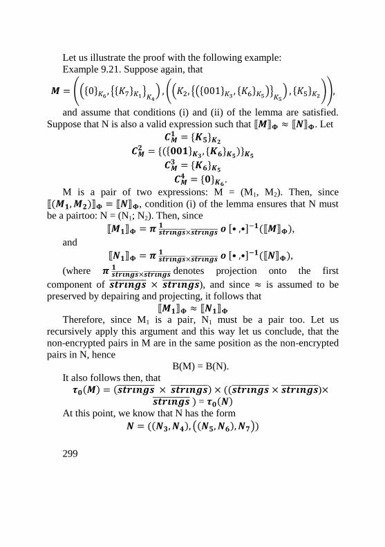
299

Let us illustrate the proof with the following example:

Example 9.21. Suppose again, that

𝑴 = (({0}𝐾6 , {{𝐾7}𝐾1}𝐾4) , ((𝐾2, {({001}𝐾3 , {𝐾6}𝐾5)}𝐾5

) , {𝐾5}𝐾2)),

and assume that conditions (i) and (ii) of the lemma are satisfied.

Suppose that N is also a valid expression such that ⟦𝑴⟧𝚽 ≈ ⟦𝑵⟧𝚽. Let

𝑪𝑴𝟏 = {𝑲𝟓}𝑲𝟐

𝑪𝑴𝟐 = {({𝟎𝟎𝟏}𝑲𝟑 , {𝑲𝟔}𝑲𝟓)}𝑲𝟓

𝑪𝑴𝟑 = {𝑲𝟔}𝑲𝟓

𝑪𝑴𝟒 = {𝟎}𝑲𝟔.

M is a pair of two expressions: M = (M1, M2). Then, since ⟦(𝑴𝟏,𝑴𝟐)⟧𝚽 = ⟦𝑵⟧𝚽, condition (i) of the lemma ensures that N must

be a pairtoo: N = (N1; N2). Then, since

⟦𝑴𝟏⟧𝚽 = 𝝅 𝒔𝒕𝒓𝒊𝒏𝒈𝒔̅̅ ̅̅ ̅̅ ̅̅ ̅̅ ̅×𝒔𝒕𝒓𝒊𝒏𝒈𝒔̅̅ ̅̅ ̅̅ ̅̅ ̅̅ ̅𝟏 𝒐 [• ,•]−𝟏(⟦𝑴⟧𝚽),

and

⟦𝑵𝟏⟧𝚽 = 𝝅 𝒔𝒕𝒓𝒊𝒏𝒈𝒔̅̅ ̅̅ ̅̅ ̅̅ ̅̅ ̅×𝒔𝒕𝒓𝒊𝒏𝒈𝒔̅̅ ̅̅ ̅̅ ̅̅ ̅̅ ̅𝟏 𝒐 [• ,•]−𝟏(⟦𝑵⟧𝚽),

(where 𝝅 𝒔𝒕𝒓𝒊𝒏𝒈𝒔̅̅ ̅̅ ̅̅ ̅̅ ̅̅ ̅×𝒔𝒕𝒓𝒊𝒏𝒈𝒔̅̅ ̅̅ ̅̅ ̅̅ ̅̅ ̅𝟏 denotes projection onto the first

component of 𝒔𝒕𝒓𝒊𝒏𝒈𝒔̅̅ ̅̅ ̅̅ ̅̅ ̅̅ ̅ × 𝒔𝒕𝒓𝒊𝒏𝒈𝒔̅̅ ̅̅ ̅̅ ̅̅ ̅̅ ̅), and since ≈ is assumed to be

preserved by depairing and projecting, it follows that

⟦𝑴𝟏⟧𝚽 ≈ ⟦𝑵𝟏⟧𝚽 Therefore, since M1 is a pair, N1 must be a pair too. Let us

recursively apply this argument and this way let us conclude, that the

non-encrypted pairs in M are in the same position as the non-encrypted

pairs in N, hence

B(M) = B(N).

It also follows then, that

𝝉𝟎(𝑴) = (𝒔𝒕𝒓𝒊𝒏𝒈𝒔̅̅ ̅̅ ̅̅ ̅̅ ̅̅ ̅ × 𝒔𝒕𝒓𝒊𝒏𝒈𝒔̅̅ ̅̅ ̅̅ ̅̅ ̅̅ ̅) × ((𝒔𝒕𝒓𝒊𝒏𝒈𝒔̅̅ ̅̅ ̅̅ ̅̅ ̅̅ ̅ × 𝒔𝒕𝒓𝒊𝒏𝒈𝒔̅̅ ̅̅ ̅̅ ̅̅ ̅̅ ̅)×𝒔𝒕𝒓𝒊𝒏𝒈𝒔̅̅ ̅̅ ̅̅ ̅̅ ̅̅ ̅ ) = 𝝉𝟎(𝑵)

At this point, we know that N has the form

𝑵 = ((𝑵𝟑, 𝑵𝟒), ((𝑵𝟓, 𝑵𝟔),𝑵𝟕))

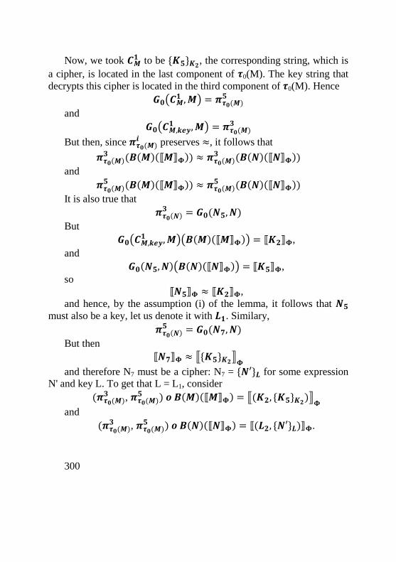
300

Now, we took 𝑪𝑴𝟏 to be {𝑲𝟓}𝑲𝟐, the corresponding string, which is

a cipher, is located in the last component of 𝝉0(M). The key string that

decrypts this cipher is located in the third component of 𝝉0(M). Hence

𝑮𝟎(𝑪𝑴𝟏 ,𝑴) = 𝝅𝝉𝟎(𝑴)

𝟓

and

𝑮𝟎(𝑪𝑴,𝒌𝒆𝒚𝟏 ,𝑴) = 𝝅𝝉𝟎(𝑴)

𝟑

But then, since 𝝅𝝉𝟎(𝑴)𝒊 preserves ≈, it follows that

𝝅𝝉𝟎(𝑴)𝟑 (𝑩(𝑴)(⟦𝑴⟧𝚽)) ≈ 𝝅𝝉𝟎(𝑴)

𝟑 (𝑩(𝑵)(⟦𝑵⟧𝚽))

and

𝝅𝝉𝟎(𝑴)𝟓 (𝑩(𝑴)(⟦𝑴⟧𝚽)) ≈ 𝝅𝝉𝟎(𝑴)

𝟓 (𝑩(𝑵)(⟦𝑵⟧𝚽))

It is also true that

𝝅𝝉𝟎(𝑵)𝟑 = 𝑮𝟎(𝑵𝟓, 𝑵)

But

𝑮𝟎(𝑪𝑴,𝒌𝒆𝒚𝟏 ,𝑴)(𝑩(𝑴)(⟦𝑴⟧𝚽)) = ⟦𝑲𝟐⟧𝚽,

and

𝑮𝟎(𝑵𝟓, 𝑵)(𝑩(𝑵)(⟦𝑵⟧𝚽)) = ⟦𝑲𝟓⟧𝚽,

so ⟦𝑵𝟓⟧𝚽 ≈ ⟦𝑲𝟐⟧𝚽,

and hence, by the assumption (i) of the lemma, it follows that 𝑵𝟓

must also be a key, let us denote it with 𝑳𝟏. Similary,

𝝅𝝉𝟎(𝑵)𝟓 = 𝑮𝟎(𝑵𝟕, 𝑵)

But then

⟦𝑵𝟕⟧𝚽 ≈ ⟦{𝑲𝟓}𝑲𝟐⟧𝚽

and therefore N7 must be a cipher: N7 = {𝑵′}𝑳 for some expression

N' and key L. To get that L = L1, consider

(𝝅𝝉𝟎(𝑴)𝟑 , 𝝅𝝉𝟎(𝑴)

𝟓 ) 𝒐 𝑩(𝑴)(⟦𝑴⟧𝚽) = ⟦(𝑲𝟐, {𝑲𝟓}𝑲𝟐)⟧𝚽

and

(𝝅𝝉𝟎(𝑴)𝟑 , 𝝅𝝉𝟎(𝑴)

𝟓 ) 𝒐 𝑩(𝑵)(⟦𝑵⟧𝚽) = ⟦(𝑳𝟐, {𝑵′}𝑳)⟧𝚽.

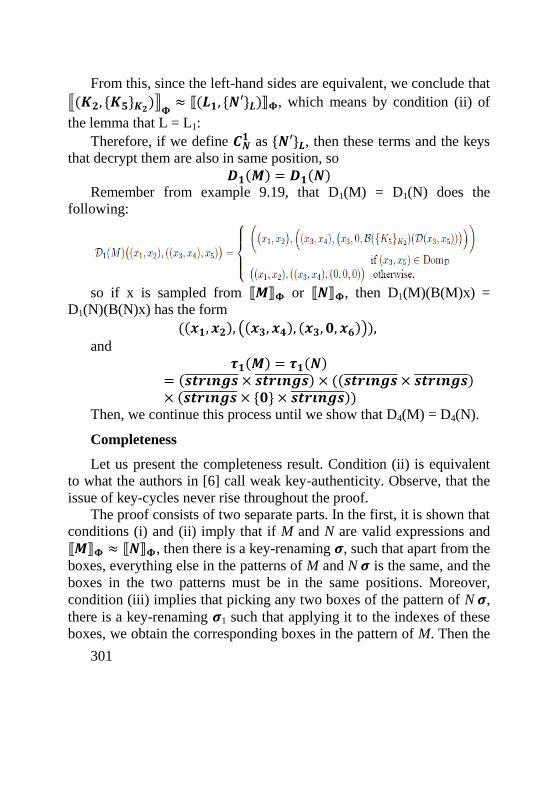
301

From this, since the left-hand sides are equivalent, we conclude that

⟦(𝑲𝟐, {𝑲𝟓}𝑲𝟐)⟧𝚽≈ ⟦(𝑳𝟏, {𝑵′}𝑳)⟧𝚽, which means by condition (ii) of

the lemma that L = L1:

Therefore, if we define 𝑪𝑵𝟏 as {𝑵′}𝑳, then these terms and the keys

that decrypt them are also in same position, so

𝑫𝟏(𝑴) = 𝑫𝟏(𝑵) Remember from example 9.19, that D1(M) = D1(N) does the

following:

so if x is sampled from ⟦𝑴⟧𝚽 or ⟦𝑵⟧𝚽, then D1(M)(B(M)x) =

D1(N)(B(N)x) has the form

((𝒙𝟏, 𝒙𝟐), ((𝒙𝟑, 𝒙𝟒), (𝒙𝟑, 𝟎, 𝒙𝟔))), and

𝝉𝟏(𝑴) = 𝝉𝟏(𝑵)= (𝒔𝒕𝒓𝒊𝒏𝒈𝒔̅̅ ̅̅ ̅̅ ̅̅ ̅̅ ̅ × 𝒔𝒕𝒓𝒊𝒏𝒈𝒔̅̅ ̅̅ ̅̅ ̅̅ ̅̅ ̅) × ((𝒔𝒕𝒓𝒊𝒏𝒈𝒔̅̅ ̅̅ ̅̅ ̅̅ ̅̅ ̅ × 𝒔𝒕𝒓𝒊𝒏𝒈𝒔̅̅ ̅̅ ̅̅ ̅̅ ̅̅ ̅)× (𝒔𝒕𝒓𝒊𝒏𝒈𝒔̅̅ ̅̅ ̅̅ ̅̅ ̅̅ ̅ × {𝟎} × 𝒔𝒕𝒓𝒊𝒏𝒈𝒔̅̅ ̅̅ ̅̅ ̅̅ ̅̅ ̅))

Then, we continue this process until we show that D4(M) = D4(N).

Completeness

Let us present the completeness result. Condition (ii) is equivalent

to what the authors in [6] call weak key-authenticity. Observe, that the

issue of key-cycles never rise throughout the proof.

The proof consists of two separate parts. In the first, it is shown that

conditions (i) and (ii) imply that if M and N are valid expressions and

⟦𝑴⟧𝚽 ≈ ⟦𝑵⟧𝚽, then there is a key-renaming 𝝈, such that apart from the

boxes, everything else in the patterns of M and N 𝝈 is the same, and the

boxes in the two patterns must be in the same positions. Moreover,

condition (iii) implies that picking any two boxes of the pattern of N 𝝈,

there is a key-renaming 𝝈1 such that applying it to the indexes of these

boxes, we obtain the corresponding boxes in the pattern of M. Then the

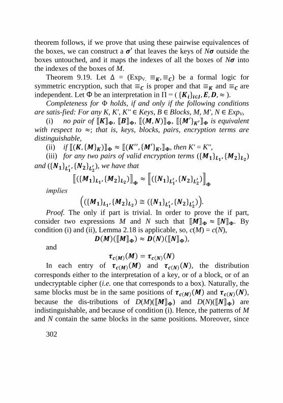
302

theorem follows, if we prove that using these pairwise equivalences of

the boxes, we can construct a 𝝈′ that leaves the keys of N𝝈 outside the

boxes untouched, and it maps the indexes of all the boxes of N𝝈 into

the indexes of the boxes of M.

Theorem 9.19. Let ∆ = (ExpV, ≡𝑲, ≡𝑪) be a formal logic for

symmetric encryption, such that ≡𝑪 is proper and that ≡𝑲 and ≡𝑪 are

independent. Let Φ be an interpretation in П = ( {𝑲𝒊}𝒊∈𝑰, 𝑬, 𝑫, ≈ ). Completeness for Φ holds, if and only if the following conditions

are satis-fied: For any K, K', K'' ∈ Keys, B ∈ Blocks, M, M', N ∈ ExpV,

(i) no pair of ⟦𝑲⟧𝚽, ⟦𝑩⟧𝚽, ⟦(𝑴,𝑵)⟧𝚽, ⟦{𝑴′}𝑲′⟧𝚽 is equivalent

with respect to ≈; that is, keys, blocks, pairs, encryption terms are

distinguishable,

(ii) if ⟦(𝑲, {𝑴}𝑲)⟧𝚽 ≈ ⟦(𝑲′′, {𝑴′}𝑲′⟧𝚽, then K' = K'',

(iii) for any two pairs of valid encryption terms ({𝑴𝟏}𝑳𝟏 , {𝑴𝟐}𝑳𝟐)

and ({𝑵𝟏}𝑳𝟏′ , {𝑵𝟐}𝑳𝟐

′ ), we have that

⟦({𝑴𝟏}𝑳𝟏 , {𝑴𝟐}𝑳𝟐)⟧𝚽≈ ⟦({𝑵𝟏}𝑳𝟏

′ , {𝑵𝟐}𝑳𝟐′ )⟧

𝚽

implies

(({𝑴𝟏}𝑳𝟏 , {𝑴𝟐}𝑳𝟐) ≅ ({𝑵𝟏}𝑳𝟏′ , {𝑵𝟐}𝑳𝟐

′ )).

Proof. The only if part is trivial. In order to prove the if part,

consider two expressions M and N such that ⟦𝑴⟧𝚽 ≈ ⟦𝑵⟧𝚽. By

condition (i) and (ii), Lemma 2.18 is applicable, so, c(M) = c(N),

𝑫(𝑴)(⟦𝑴⟧𝚽) ≈ 𝑫(𝑵)(⟦𝑵⟧𝚽), and

𝝉𝒄(𝑴)(𝑴) = 𝝉𝒄(𝑵)(𝑵)

In each entry of 𝝉𝒄(𝑴)(𝑴) and 𝝉𝒄(𝑵)(𝑵), the distribution

corresponds either to the interpretation of a key, or of a block, or of an

undecryptable cipher (i.e. one that corresponds to a box). Naturally, the

same blocks must be in the same positions of 𝝉𝒄(𝑴)(𝑴) and 𝝉𝒄(𝑵)(𝑵),

because the dis-tributions of D(M)(⟦𝑴⟧𝚽) and D(N)(⟦𝑵⟧𝚽) are

indistinguishable, and because of condition (i). Hence, the patterns of M

and N contain the same blocks in the same positions. Moreover, since

303

D(M)(⟦𝑴⟧𝚽) and D(N)(⟦𝑵⟧𝚽) are indistinguishable, the entries in

𝝉𝒄(𝑴)(𝑴) and in 𝝉𝒄(𝑵)(𝑵) containing strings sampled from key

generation must be in the same places because of (i) again.

Furthermore, the indistinguishability of 𝝉𝒄(𝑴)(𝑴) and 𝝉𝒄(𝑵)(𝑵)also

implies that repetitions of a key generation outcome must occur in the

same positions of 𝝉𝒄(𝑴)(𝑴) and 𝝉𝒄(𝑵)(𝑵) as well. (This is a

consequence of the properties of key-generation in definition 2.29.)

Therefore the key symbols in the patterns of M and N change together,

so it is possible to rename the recoverable keys of N (with a ≡𝑲

preserving function 𝝈 so that the keys in the pattern of N𝝈 are the same

as the keys in the pattern of M.

Since the distributions of D(M)(⟦𝑴⟧𝚽) and D(N)(⟦𝑵⟧𝚽) are

indistinguishable, condition (i) implies that the undecryptable ciphers

occur in exactly the same entries in 𝝉𝒄(𝑴)(𝑴) and 𝝉𝒄(𝑵)(𝑵). This

means, that in the pattern of M and N, the boxes appear in the same

position. This together with the conclusions of the previous paragraph

means, that apart from the boxes, everything else in the pattern of M

and of N𝝈 must be the same. By replacing N with N𝝈, we can assume

from now on that the recoverable keys of N and M are identical, and

that the pattern of M and N are the same outside the boxes. Therefore,

we only have to show that there is a key renaming 𝝈' that carries the

boxes of N into the boxes of M without changing the recoverable keys.

Suppose that there are l boxes altogether in the pattern of M (and

hence in the pattern of N). Let {𝑴𝟏}𝑳𝟏 , {𝑴𝟐}𝑳𝟐 , … , {𝑴𝒍}𝑳𝒍 be the l

undecryptable terms in M that turn into boxes (in M) and

{𝑵𝟏}𝑳𝟏′ , {𝑵𝟐}𝑳𝟐

′ , … , {𝑵𝒍}𝑳𝒍′ the corresponding undecryptable terms in N.

We denote by 𝝁𝒊 and 𝒗𝒊 the equivalence classes of {𝑴𝒊}𝑳𝒊 and {𝑵𝒊}𝑳𝒊′ ,

respectively, with respect to ≡𝑪. Then, as we showed above, we have

that for 𝒊, 𝒋 ≤ 𝒍, 𝒊 ≠ 𝒋,

⟦({𝑴𝒊}𝑳𝒊 , {𝑴𝒋}𝑳𝒋)⟧𝚽

≈ ⟦({𝑵𝒊}𝑳𝒊′ , {𝑵𝒋}𝑳𝒋

′ )⟧𝚽

304

holds since D(M)( ⟦𝑴⟧𝚽) and D(N)( ⟦𝑵⟧𝚽)) are indistinguishable,

and thus, by condition (iii),

({𝑴𝒊}𝑳𝒊 , {𝑴𝒋}𝑳𝒋) ≅ ({𝑵𝒊}𝑳𝒊

′ , {𝑵𝒋}𝑳𝒋′).

So, by definition of ≅ , there exists a key-renaming 𝝈𝒊,𝒋 such that

( 𝝁𝒊 , 𝝁𝒋) = ( 𝝈𝒊,𝒋(𝒗𝒊), 𝝈𝒊,𝒋(𝒗𝒋)

),

that is, there exists a key-renaming 𝝈𝒊,𝒋 such that

𝝁𝒊 = 𝝈𝒊,𝒋(𝒗𝒊) and 𝝁𝒊 = 𝝈𝒊,𝒋(𝒗𝒋) (9.10)

Consider now the class 𝑪 = {{𝑵𝒊}𝑳𝒊′ }𝒊=𝟏𝒍 . Since we assumed by

hypothesis that ≡𝑪 is proper, by Proposition 2.13 (using S = R-Keys(N)

and noticing that 𝑳𝒌′ ∉ R-Keys(N)) we have that for each 𝒗𝒌,

equivalence class of {𝑵𝒌}𝑳𝒌′ , there is a representative C𝒗𝒌 such that:

(i) Keys(C𝒗𝒌) ⋂ R-Keys(N) = ∅,

(ii) 𝑳𝒎′ 𝑪𝒗𝒌 for all m ∈ {𝟏, 𝟐,… , 𝒍}.

(iii) if 𝒗𝒌𝟏 ≠ 𝒗𝒌𝟐 , |(𝒗𝒌𝟏)𝒌𝒆𝒚| ≠ ∞ and |(𝒗𝒌𝟐)𝒌𝒆𝒚| ≠

∞, 𝒕𝒉𝒆𝒏 𝑲𝒆𝒚𝒔(𝑪𝒗𝒌𝟏) ⋂𝑲𝒆𝒚𝒔(𝑪𝒗𝒌𝟐

) ≠ ∅ if and only if (𝒗𝒌𝟏)𝒌𝒆𝒚 =

(𝒗𝒌𝟐)𝒌𝒆𝒚 = {𝑲} for some key K, and in that case

4. Keys(𝑪𝒗𝒌𝟏) ⋂ Keys(𝑪𝒗𝒌𝟐

) = {𝑲},

5. 𝑪𝒗𝒌𝟏 and 𝑪𝒗𝒌𝟐

are both of the form {•}𝑲, and

6. K 𝑪𝒗𝒌𝟏, K 𝑪𝒗𝒌𝟐

.

(iv) if 𝒗𝒌𝟏 ≠ 𝒗𝒌𝟐 and either |(𝒗𝒌𝟏)𝒌𝒆𝒚|= ∞, or |(𝒗𝒌𝟐)𝒌𝒆𝒚|

=

∞then 𝑲𝒆𝒚𝒔 (𝑪𝒗𝒌𝟏) ⋂𝑲𝒆𝒚𝒔 (𝑪𝒗𝒌𝟐

) ≠ ∅

Let us define the key-renaming function 𝝉 that leaves the

recoverable keys of M (and N) untouched but that maps the boxes in the

pattern of N to the corresponding boxes in the pattern of M. This

definition is done by induction.

305

Induction Basis: Let us start by defining 𝝉𝟐𝟑. Since we assumed that

≡𝑪 and ≡𝑲 are inde-pendent, it is possible to modify 𝝈𝟏,𝟐 such that the

resulting renaming function 𝝉𝟐 that we get leaves

𝑺𝟐 = ( ⋃𝑲𝒆𝒚𝒔(𝑪𝒗𝒊) ∪ 𝑹 − 𝑲𝒆𝒚𝒔(𝑵)(𝑲𝒆𝒚𝒔(𝑪𝒗𝟏) ∪ 𝑲𝒆𝒚𝒔(𝑪𝒗𝟐))

𝒍

𝒊=𝟑

untouched and is such that

𝝉𝟐(𝒗𝟏) = 𝝈𝟏,𝟐(𝒗𝟏) and 𝝉𝟐(𝒗𝟐) = 𝝈𝟏,𝟐(𝒗𝟐) If we combine the previous equations with (2.10) we have that

𝝉𝟐(𝒗𝟏) = 𝝈𝟏,𝟐(𝒗𝟏) = 𝝁𝟏

and

𝝉𝟐(𝒗𝟐) = 𝝈𝟏,𝟐(𝒗𝟐) = 𝝁𝟐.

Induction Hypothesis: Suppose now that we have defined the keys

in ¿k in a such a way that ¿k leaves

𝑺𝒌 = ( ⋃ 𝑲𝒆𝒚𝒔(𝑪𝒗𝒊) ∪

𝒍

𝒊=𝒌+𝟏

𝑹−𝑲𝒆𝒚𝒔(𝑵) ) \ ( ⋃𝑲𝒆𝒚𝒔(𝑪𝒗𝒊)

𝒌

𝒊=𝟏

),

untouched and is such that

𝝉𝒌(𝒗𝒊) = 𝝁𝒊 for all 𝒊 ≤ 𝒌

Inductive Step: There are two cases. First suppose that 𝒗𝒌+𝟏 = 𝒗𝒊 for some 𝒊 ≤ 𝒌. In this case, we define 𝝉𝒌+𝟏 = 𝝉𝒌. It is obvious that

𝝉𝒌+𝟏 leaves the keys of

𝑺𝒌+𝟏 = ( ⋃ 𝑲𝒆𝒚𝒔(𝑪𝒗𝒊) ∪

𝒍

𝒊=𝒌+𝟐

𝑹−𝑲𝒆𝒚𝒔(𝑵) ) \ ( ⋃𝑲𝒆𝒚𝒔(𝑪𝒗𝒊)

𝒌+𝟏

𝒊=𝟏

),

untouched and is such that

𝝉𝒌+𝟏(𝒗𝒊) = 𝝁𝒊 for all 𝒊 ≤ 𝒌 + 𝟏

since 𝑪𝒗𝒌+𝟏 = 𝑪𝒗𝒊 and 𝒗𝒌+𝟏 = 𝒗𝒊.

In the other case, suppose that 𝒗𝒌+𝟏 ≠ 𝒗𝒊 for all 𝒊 ≤ 𝒌. Consider

now the substitution 𝝈𝒋,(𝒌+𝟏) with 𝒋 ≤ 𝒌. By (9.10) we have that

𝝁𝒋 = 𝝈𝒋,(𝒌+𝟏)(𝒗𝒋)

and

306

𝝁𝒌+𝟏 = 𝝈𝒋,(𝒌+𝟏)(𝒗𝒌+𝟏).

Since ≡𝑪 and ≡𝑲 are independent, considering

𝑺 = (⋃𝑲𝒆𝒚𝒔(𝑪𝒗𝒊) ∪ 𝝉𝒌

𝒍

𝒊=𝟏

(⋃𝑲𝒆𝒚𝒔(𝑪𝒗𝒊)

𝒍

𝒊=𝟏

) ∪ 𝐑 − 𝐊𝐞𝐲𝐬(𝐍))

\𝑲𝒆𝒚𝒔(𝑪𝒗𝒌+𝟏)

And 𝑪 = {𝑪𝒗𝒌+𝟏}, we have that it is possible to modify 𝝈𝒋,(𝒌+𝟏) to

𝝈∗ such that

𝝈∗(K) = K for all K ∈ S

and

𝝈∗(𝒗𝒌+𝟏) = 𝝈𝒋,(𝒌+𝟏)(𝒗𝒌+𝟏)

Using (9.12), we can rewrite the previous equation as

𝝈∗(𝒗𝒌+𝟏) = 𝝈𝒋,(𝒌+𝟏)(𝒗𝒌+𝟏) = 𝝁𝒌+𝟏

Thus, we have two substitutions, 𝝉𝒌 and 𝝈∗ such that

𝝉𝒌(𝒗𝒊) = 𝝁𝒊 for all 𝒊 ≤ 𝒌 (9.13)

and

𝝈∗(𝒗𝒌+𝟏) = 𝝁𝒌+𝟏 (9.14)

Our goal now is to combine these two substitutions into one

substitution 𝝉𝒌+𝟏 such that

𝝉𝒌+𝟏(𝒗𝒊) = 𝝁𝒊 for all 𝒊 ≤ 𝒌 + 𝟏 (9.15)

and that leaves untouched the keys in

𝑺𝒌+𝟏 = ( ⋃ 𝑲𝒆𝒚𝒔(𝑪𝒗𝒊) ∪

𝒍

𝒊=𝒌+𝟐

𝑹−𝑲𝒆𝒚𝒔(𝑵) ) \ ( ⋃𝑲𝒆𝒚𝒔(𝑪𝒗𝒊)

𝒌+𝟏

𝒊=𝟏

),

We can immediately notice that by definition, 𝝉𝒌 only changes the

keys in (⋃ 𝑲𝒆𝒚𝒔(𝑪𝒗𝒊)𝒌𝒊=𝟏 ) (recall (9.11)) and that 𝝈∗ only alters the

keys in Keys(𝑪𝒗𝒌+𝟏), thus ensuring (9.16). We also notice that from

(9.13) and (9.14), (9.15) follows. So, if it is possible to “merge” the two

substi-tutions, the result follows. We do this by showing that the two

substitutions are compatible. We show that if both substitutions change

the value of one key K, then they change it to the same value, that is,

307

we show that if for a key K, 𝝉𝒌(𝑲) ≠ 𝑲 and 𝝈∗(𝑲) ≠ 𝑲 then 𝝉𝒌(𝑲) =𝝈∗(𝑲).

Suppose that both 𝝉𝒌 and 𝝈∗ change the value of a key K'. Then, by

the definition of the two substitutions,

𝑲′(⋃𝑲𝒆𝒚𝒔(𝑪𝒗𝒊)

𝒌

𝒊=𝟏

)⋂ 𝑲𝒆𝒚𝒔(𝑪𝒗𝒌+𝟏).

that is

𝑲′ ∈ 𝑲𝒆𝒚𝒔(𝑪𝒗𝒊) ⋂ 𝐊𝐞𝐲𝐬(𝑪𝒗𝒊)

for some i ∈ {𝟏,… , 𝒌}. By the way we constructed the

representatives 𝑪𝒗𝒌 we have that foe any two different equivalence

classes 𝒗𝒌𝟏 and 𝒗𝒌𝟐, 𝑲𝒆𝒚𝒔(𝑪𝒗𝒊)⋂𝑲𝒆𝒚𝒔(𝑪𝒗𝒊) = ∅ (whenever

|(𝒗𝒊)𝒌𝒆𝒚| = ∞ or |(𝒗𝒌+𝟏)𝒌𝒆𝒚| = ∞) or

𝑲𝒆𝒚𝒔 (𝑪𝒗𝒌𝟏)⋂𝑲𝒆𝒚𝒔(𝑪𝒗𝒌𝟐

) ≠ ∅ if and only if (𝒗𝒌𝟏)𝒌𝒆𝒚 =

(𝒗𝒌𝟐)𝒌𝒆𝒚 = {𝑲}, and in that case

𝑲𝒆𝒚𝒔(𝑪𝒗𝒌𝟏)⋂𝑲𝒆𝒚𝒔(𝑪𝒗𝒌𝟐

) = {𝑲}.

Since {𝑵𝒊}𝑳𝒊′ ∈ 𝒗𝒊 and {𝑵𝒌+𝟏}𝑳𝒌+𝟏

′ ∈ 𝒗𝒌+𝟏, we have that 𝑳𝒊′ ∈

(𝒗𝒊)𝒌𝒆𝒚 and 𝑳𝒌+𝟏′ ∈ (𝒗𝒌+𝟏)𝒌𝒆𝒚, and using (2.18) it follows that

𝑲′ = 𝑳𝒊′ = 𝑳𝒌+𝟏

′ .

We just proved that the only key that both 𝝉𝒌 and 𝝈∗ change at the

same time is K' so we just need to prove that they change it to the same

value (in order to be compatible), that is,

𝝉𝒌(𝑲′) = 𝝈∗(𝑲′).

By (9.18) we have that |(𝒗𝒌+𝟏)𝒌𝒆𝒚| = 𝟏 and so, using Proposition

9.12 and (9.14) it follows that

|(𝝁𝒌+𝟏)𝒌𝒆𝒚| = |𝝈∗((𝒗𝒌+𝟏)𝒌𝒆𝒚)| = 𝟏 .

Since {𝑴𝒌+𝟏}𝑳𝒌+𝟏 ∈ 𝝁𝒌+𝟏 , we have that 𝑳𝒌+𝟏 ∈ (𝝁𝒌+𝟏)𝒌𝒆𝒚. So,

from the previous equation and (9.18) it follows that

𝝈∗(𝑲′) = 𝝈∗(𝑳𝒌+𝟏′ ) = 𝑳𝒌+𝟏 (9.20)

308

If we apply the same reasoning to 𝒗𝒊 and 𝝉𝒌, again by (9.18) we

have that |(𝒗𝒊)𝒌𝒆𝒚| = 𝟏 and so, using Proposition 9.12 and (9.13) it

follows that

|(𝝁𝒊)𝒌𝒆𝒚| = |𝝉𝒌((𝒗𝒊)𝒌𝒆𝒚)| = 𝟏.

Since {𝑴𝒊}𝑳𝒊 , ∈ 𝝁𝒊, we have that 𝑳𝒊 ∈ (𝝁𝒊)𝒌𝒆𝒚. So, from the

previous equation and (2.18) it follows that

𝝉𝒌(𝑲′) = 𝝉𝒌(𝑳𝒊

′) = 𝑳𝒊 (9.21)

Now consider the substitution 𝝈𝒊,(𝒌+𝟏). By (9.10) we have that

𝝁𝒊 = 𝝈𝒊,(𝒌+𝟏)(𝒗𝒊) and 𝝁𝒌+𝟏 = 𝝈𝒊,(𝒌+𝟏)(𝒗𝒌+𝟏). Using (9.18) and Proposition 9.2 it follows that

|(𝝁𝒊)𝒌𝒆𝒚| = |𝝈𝒊,(𝒌+𝟏)((𝒗𝒊)𝒌𝒆𝒚)| = 1 and |(𝝁𝒊)𝒌𝒆𝑦| =

|𝝈𝒊,(𝒌+𝟏)((𝒗𝒌+𝟏)𝒌𝒆𝒚)| = 1

As said before, 𝑳𝒊 ∈ (𝝁𝒊)𝒌𝒆𝒚, 𝑳𝒊′ ∈ (𝒗𝒊)𝒌𝒆𝒚, 𝑳𝒌+𝟏 ∈

(𝝁𝒌+𝟏)𝒌𝒆𝒚, and 𝑳𝒌+𝟏′ ∈ (𝒗𝒌+𝟏)𝒌𝒆𝒚 and so

𝝈𝒊,(𝒌+𝟏)(𝑳𝒊′) = 𝑳𝒊 𝒂𝒏𝒅 𝝈𝒊,(𝒌+𝟏)(𝑳𝒌+𝟏

′ ) = 𝑳𝒌+𝟏

Combining this with (9.19), since 𝑳𝒊′ = 𝑳𝒌+𝟏

′ , we have that

𝑳𝒊 = 𝑳𝒌+𝟏 and so by (9.21), (9.22), and (9.20)

𝝉𝒌(𝑲′) = 𝑳𝒊 = 𝑳𝒌+𝟏 = 𝝈

∗(𝑲′). Thus for any key K' such that both 𝝉𝒌 and 𝝈∗ change the value, they

are compatible. We then define 𝝉𝒌+𝟏 as i\; S

𝝉𝒌+𝟏(𝑲) = {𝝈∗(𝑲) 𝒊𝒇 𝑲 ∈ 𝑲𝒆𝒚𝒔(𝑪𝒗𝒌+𝟏)

𝝉𝒌(𝑲) 𝒐𝒕𝒉𝒆𝒓𝒘𝒊𝒔𝒆,

Note that by definition og 𝝉𝒍, it does not change the keys in

𝑺𝒍 = 𝑹−𝑲𝒆𝒚𝒔(𝑵)\(⋃ 𝑲𝒆𝒚𝒔𝒍𝒊=𝟏 (𝑪𝒗𝒊)) but, by properness, we

have that 𝑲𝒆𝒚𝒔(𝑪𝒗𝒊)𝑹 −𝑲𝒆𝒚𝒔(𝑵) = ∅ for all 𝟏 ≤ 𝒊 ≤ 𝒍 which

implies that 𝝉𝒍 does not the keys in R-Keys(N).

The substitution 𝝉 that satisfies the required properties, i.e., that

leaves the recoverable keys of M and N untouched, but maps the boxes

of the pattern of N into the corresponding boxes in the pattern of M, is

309

defined as 𝝉𝒍 (l is the number of boxes in the pattern of M) and that is

what we needed to complete the proof.

Remark 9.4. Observe, that condition (iii) of the theorem is trivially

satisfied when there is only one box, that is, when all encryption terms

are equivalent under ≡𝐶. Also, if completeness holds for a certain

choice of ≡𝐶, then, if ≡𝐶′ is such that M ≡𝐶 N implies M ≡𝐶

′ N—i.e.

when ≡𝐶′ results fewer boxes—then completeness holds for ≡𝐶

′ as well.

Therefore, we can say, that the key to completeness is not to have too

many boxes.

Example 9.22 (Completeness for Type-1 and Type-2 Encryption

Schemes). The complete-ness part of our earlier theorems for type-1

and type-2 encryption schemes are clearly special cases of this theorem,

because the formal language we introduced for these schemes were

such that ≡𝐶 is proper and ≡𝐾 and ≡𝐶 are independent, and the

conditions of the theorems are anal-ogous.

Example 9.23 (Completeness for One-Time Pad). The formal logic

for OTP is such that ≡𝐶 is proper and ≡𝐾 and ≡𝐶 are independent.

Furthermore, con-dition (i) of. Condition (ii) is also satisfied because of

the tagging: the reason ultimately is that decrypting with the wrong key

will sometimes result invalid endings. Condition (iii) is also satisfied,

since the pairs of encryption terms must be encrypted with different

keys (in OTP, we cannot use the keys twice), and the equivalence

⟦({𝑀1}𝐿1 , {𝑀2}𝐿2)⟧Φ≈ ⟦({𝑁1}𝐿1′ , {𝑁2}𝐿2′ )⟧Φ

implies that the

corresponding lengths in the two encryption terms wust be the same:

𝑙({𝑀1}𝐿1) = 𝑙({𝑁1}𝐿1′ ) and 𝑙({𝑀2}𝐿2) = 𝑙({𝑁2}𝐿2′ ) which implies

( 𝑙({𝑀1}𝐿1), ({𝑀2}𝐿2)

) = (𝑙({𝑁1}𝐿1

′ ),

𝑙({𝑁2}𝐿2′ )

). Therefore,

({𝑀1}𝐿1 , {𝑀2}𝐿2) ≅ ({𝑁1}𝐿1′ , {𝑁2}𝐿2′ ). In conclusion, the formal logic is

complete.

310

Advancement questions

1. What are the main conditions of the Abadi-Rogaway

Soundness Theorem?

2. What are the main features of the AR Equivalence of Formal

Expressions?

3. Through what the equivalence of expressions is able to be

obtained?

4. What does KDM security mean?

5. Why does the soundness in the presence of key-cycles is not

possible to prove with the security notion adopted by Abadi

and Rogaway?

6. Why does type-0 security is not strong enough to ensure

soundness in the case of key-cycles?

7. What are the features of the ‘type-1’ encryption schemes?

8. What does type-1 encryption in the terminology of Abadi and

Rogaway mean?

9. What is the difference between the type-1 and type-2

encryptions?

10. Why does it possible to construct encryption schemes that are

type-0, but fail to provide soundness in the presence of key-

cycles?

REFERENCES

[1] Pedro Miguel dos Santos Alves Madeira Adao Formal

methods for the analysis of security protocols / Pedro Miguel dos

Santos Alves Madeira Adao // PhD thesis . – 2006. – Universidad et

Tecnica de Lisboa Instituto Superior Tecnico.

[2] M. Abadi Reconciling two views of cryptography (the

computational soundness of formal encryption) / M. Abadi , P.

Rogaway // Journal of Cryptology. – 2002. - 15(2). Pp.103–127.

311

[3] J. Black Encryption-scheme security in the presence of key-

dependent messages / J. Black, P. Rogaway, T. Shrimpton // Lecture

Notes in Computer Science. – 2002 - Volume 259 – pp.62–75.

[4] M. Abadi Reconciling two views of cryptography / M.

Abadi, P. Rogaway // Lecture Notes in Computer Scien. – 2000. – vol.

1872. – pp. 3–22.

[5] J. Camenisch An efficient system for non-transferable

anonymous credentials with optional anonymity revocation / J.

Camenisch and A. Lysyanskaya // Lecture Notes in Computer Science.

– 2001. - volume 2045. – pp. 98–118.

[6] O. Horvitz Weak key authenticity and the computational

completeness of formal encryption / O. Horvitz and V. Gligor // Boneh.

- pages 530–547.

[7] A. C. Yao. Theory and applications of trapdoor functions / A.

C. Yao // In 23rd IEEE Symposium on Foundations of Computer

Science (FOCS). – 1982 . – pp. 80–91.

1

PART 3. FORMAL AND INTELLECTUAL METHODS

FOR SYSTEM SECURITY AND RESILIENCE

Content of the PART3

GLOSSARY ...................................................................................... 8

PART 3. Formal and Intellectual Methods for System Security and

Resilience .......................................................................................... 1

Content of the PART3 ....................................................................... 1

CHAPTER 10. Process Algebras for Studying Security ................... 6

Content of the CHAPTER 10 ............................................................ 6

Introduction ..................................................................................... 10

10.1 Low-Level Target Model ......................................................... 11

10.2 A Distributed Calculus with Principals and Authentica-tion ... 13

Syntax and Informal Semantics ....................................................... 13

Operational Semantics ..................................................................... 17

Local Reductions ............................................................................. 17

System Transitions .......................................................................... 18

Compositionality ............................................................................. 21

An Abstract Machine for Local Reductions .................................... 22

10.3 High-Level Equivalences and Safety ....................................... 23

Bounding processes ......................................................................... 26

Equivalences with Message Authentication; Strong Secrecy and

Authentication ................................................................................. 28

Equivalences with Certificates ........................................................ 28

10.4 Applications ............................................................................. 29

Anonymous Forwarders .................................................................. 29

2

Electronic Payment Protocol ........................................................... 30

Initialisation ..................................................................................... 33

10.5 A Concrete Implementation ..................................................... 35

Implementation of Machines ........................................................... 36

Low-level Processes Reductions ..................................................... 38

Marshaling and Unmarshaling Protocols......................................... 38

Sending and Receiving Protocols .................................................... 40

Mapping High-Level Systems to Low-Level Machines .................. 41

10.11 Main Results .......................................................................... 44

CHAPTER 11. A Process Algebra for Reasoning About Quantum

Security ............................................................................................ 51

Content of the chapter 11................................................................. 51

Introduction ..................................................................................... 52

11.1 Process Algebra ....................................................................... 52

11.2 Quantum polynomial machines .............................................. 52

11.3 Process algebra ........................................................................ 59

11.4 Semantics ................................................................................. 62

11.4 Observations and observational equivalence ........................... 65

11.6 Emulation and Composition Theorem ..................................... 67

11.7 Quantum Zero-Knowledge Proofs ........................................... 69

CHAPTER 12. Intellectual methods for security ............................ 73

Content of the PART3 ..................................................................... 73

12.1 Application of Artificial Intelligence in Network Intrusion

Detection .......................................................................................... 77

Introduction ..................................................................................... 77

3

Background Knowledge .................................................................. 77

Overview of Some Artificial Intelligence Techniques and their

Application in IDS ........................................................................... 81

Advances in Artificial Intelligence Hybrid and Ensemble

Techniques in IDS ........................................................................... 88

12.2 Multi-agent based approach of botnet detection in computer

systems ............................................................................................ 90

Multi-agent system of botnet detection ........................................... 93

Sensor of botnet detection in monitor mode .................................... 96

Sensor of botnet detection in scanner mode .................................... 99

Agents’ functioning ......................................................................... 99

Experiments ................................................................................... 101

12.3 Technique for bots detection which use polymorphic code .. 102

Related works ................................................................................ 103

Background .................................................................................... 104

Technique for bots detection which use polymorphic code .......... 105

Levels of polymorphism ................................................................ 106

The first level of polymorphism .................................................... 106

The second level of polymorphism ............................................... 107

The third/fourth levels of polymorphism ....................................... 108

The fifth level of polymorphism .................................................... 109

The sixth level of polymorphism ................................................... 110

Polymorhic code detection sensor ................................................. 111

Experiments ................................................................................... 115

Conclusions ................................................................................... 116

4

CHAPTER 13. Methods and Techniques for Formal Development and

Quantitative Assessment. Resilient systems .................................. 125

Content of the chapter 13............................................................... 125

Background: Concepts ................................................................... 126

Resilience Concept ........................................................................ 126

Dependability: Basic Definitions ................................................... 127

Goal-Based Development .............................................................. 130

System Autonomy and Reconfiguration ........................................ 131

Methods and Techniques for Formal Development and Quantitative

Assessment .................................................................................... 133

Development Methodologies ......................................................... 133

Event-B Method ............................................................................ 135

Quantitative Assessment................................................................ 140

PRISM model checker ................................................................... 141

Discrete-event simulation .............................................................. 142

CHAPTER 14. Formal Development and Quantitative Assessment of

Resilient Distributed Systems ........................................................ 155

Content of the chapter 14............................................................... 155

14.1 Overview of the Proposed Approach ..................................... 156

14.2 Resilience-Explicit Development Based on Functional

Decomposition. .............................................................................. 160

14.3 Modelling Component Interactions with Multi-Agent

Framework ..................................................................................... 166

14.4 Goal-Oriented Modelling of Resilient Systems ..................... 173

14.5 Pattern-Based Formal Development of Resilient MAS ......... 173

5

14.6 Formal Goal-Oriented Reasoning About Resilient Re-

configurable MAS ......................................................................... 180

14.7 Modelling and Assessment of Resilient Architectures .......... 185

10 PROCESS ALGEBRAS FOR STUDYING SECURITY

8

GLOSSARY

PPT - probabilistic polynomial-time

QRAM - a quantum random access machine

QPM - a quanlum polynomil machine

RAM - random access machine

RSA algorithm – Rivest’s, Shamir’s and Adleman’s algorithm

IDS - Intrusion Detection System

AI - Artificial Intelligence

ANN - Artificial Neural Networks

SVM - Support Vector Machines

GA - Genetic Algorithms

FNN - Fuzzy Neural Networks

CI - Computational Intelligence

DM - Data Mining

FS - Fuzzy System

MF - Membership Function

DOS - Denial of Service

R2L - Remote to User

U2R - User to Root

SVMs - Support Vector Machines

SVR - Support Vector Regression

SVs - Support Vectors

GA - Genetic Algorithm

FN - Functional Networks

FNN - a Fuzzy Neural Network

SVM - Support Vector Machines

T2FL - Type-2 Fuzzy Logic

FFS - FN-Fuzzy Logic-SVM

FSF - FN-SVM-Fuzzy Logic

LP - Linear Programming

CS - computer system

10 PROCESS ALGEBRAS FOR STUDYING SECURITY

9

CFG - control flow graph

CS - computer system

AMAS - antiviral multi-agent system

DTMC - discrete time Markov chains

CTMC - continuous-time Markov chains

MDP - Markov decision processes

PCTL - Probabilistic Computation Tree Logic

CSL - Continuous Stochastic Logic

WAL - Write-ahead logging

10 PROCESS ALGEBRAS FOR STUDYING SECURITY

10

Introduction

Process Algebras have been widely used in the study of security of

concurrent systems [1-9]. In spite of their success in proving security of

cryptographic protocols, mainly secrecy and authenticity properties, all

these are stated in the so called Dolev-Yao Model, hence no real

cryptographic guarantees are achieved.

Another approach is to supplement process calculi with concrete

probabilistic or polynomi-al-time semantics [18]. Unavoidably,

reasoning on processes becomes more difficult.

In this Chapter, we present a process calculus that enjoys both the

simplicity of an abstract symbolic model and a concrete (sound and

complete) implementation that achieves strong cryp-tographic

guarantees. Our calculus is a variant of the pi calculus with high level

security prim-itives; it provides name mobility, reliable messaging and

authentication primitives, but neither explicit cryptography nor

probabilistic behaviours.

Taking advantage of concurrency theory, it supports simple

reasoning, based on labelled transitions and observational equivalence.

This chapter presents its concrete implementation in a computational

setting. The implementation relies on standard cryptographic

primitives, compu-tational security definitions (CCA2 for encryption

[10], CMA for signing [11], recalled in Appendix A), and networking

assumptions. It also combines typical distributed implemen-tation

mechanisms such as abstract machines, marshaling and unmarshaling,

multiplexing, and basic communications protocols.

We establish general completeness results in the presence of active

probabilistic polynomial-time adversaries, for both trace properties and

observational equivalences, essentially showing that high level

reasoning accounts for all low-level adversaries.

This chapter illustrates the approach by coding security protocols

and establishing their computational correctness by simple formal

reasoning.

This Chapter is organised as follows: it starts by describing the low-

level target model as the constraints imposed by this will drive the

design of the high-level language, then high-level language and

semantics is presented, and notion of high-level equivalence are defined

10 PROCESS ALGEBRAS FOR STUDYING SECURITY

11

and illustrated. Chapter is also devoted to applications. Anonymous

forwarders in the language and exhibit an example of an electronic

payment protocol are encoded. As an example the encoding of an

initialisation protocol is given, that is, given any system S that possibly

shares names and certificates among principals, we can always find an

initial system 𝑆о where principals share no information, such that there

is a transition from 𝑆о to S. Chapter describes concrete implementation,

and results.

10.1 Low-Level Target Model

Before presenting the language design and implementation, let us

specify the target systems. Let us do this, as the design of our language

is, in part, driven by the target model. We have to be as abstract as

possible, but at the same time we need to faithfully abstract the

properties of the computational implementation.

As an example, we want our high-level environments to have the

same capabilities as the low-level adversaries, that are probabilistic

polynomial-time (PPT) cryptographic algorithms. We follow the

conservative assumption that an adversary controls all network traffic:

it can intercept, delay, or even block permanently any communication

between principals. For that, we cannot guarantee message delivery,

nor implement private channels that prevent traffic analysis. Reflect-ing

this in the high-level semantics implies that the simple pi-calculus rule

𝑐̅⟨𝑀⟩. 𝑃 | 𝑐(𝑥). 𝑄 → 𝑃 | 𝑄{𝑀/𝑥}, which models silent communication

is too abstract for our purposes. (Consider P and Q two processes that

are implemented in two separate machines connected by a public net-

work, and even if c is a restricted channel, the adversary can simply

block all communications.)

We consider systems that consist of a finite number of principals

𝑎, 𝑏, 𝑐, 𝑒, 𝑢, 𝑣, … ∈ Prin. Each principal a runs its own program, written

in our high-level language and executed by the PPT machine Ma

defined in Section 3.5. Each machine Ma has two wires, ina and outa,

rep-resenting a basic network interface. When activated, the machine

reads a bitstring from ina, performs some local computation, then writes

a bitstring on outa and yields. The machine em-beds probabilistic

algorithms for encryption, signing, and random-number generation—

thus the machine outputs are random variables. The machine is also

10 PROCESS ALGEBRAS FOR STUDYING SECURITY

12

parameterised by a security parameter η ∈ ℕ —intuitively, the length

for all keys—thus these outputs are ensembles of probabilities.

Some of these machines may be corrupted, under the control of the

attacker; their implemen-tation is then unspecified and treated as part of

the attacker. We let 𝑎, 𝑏, 𝑐 ∈ 𝐻 with H ⊂ Prin range over principals

that comply with our implementation, and let 𝑀 = (𝑀𝑎)𝑎∈𝐻 describe

the whole system. We denote by e a principal controlled by the

adversary ( 𝑒 ∈ 𝑃𝑟𝑖𝑛\𝐻) and by u, v an arbitrary principal in Prin. Of

course, when a interacts with 𝑢 ∈ 𝑃𝑟𝑖𝑛, its implementation Ma does not

know whether 𝑢 ∈ 𝐻 or not.

The adversary, A, is a PPT algorithm that controls the network, the

global scheduler, and some compromised principals. At each moment,

only one machine is active: whenever an ad-versary delivers a message

to a principal, the machine for this principal is activated, runs until

completion, and yields an output to the adversary. We have then the

following definition:

Definition 10.1 (Run). We define a run of A and M with security

parameter η ∈ ℕ as follows:

- key materials, with security parameter η , are generated for every

principal 𝑎 ∈ 𝑃𝑟𝑖𝑛;

- every Ma is activated with 1η, the keys for a, and the public keys

for all 𝑢 ∈ 𝑃𝑟𝑖𝑛;

- A is activated with 1η, the keys for 𝑒 ∈ 𝑃𝑟𝑖𝑛\𝐻, and the public

keys for 𝑎 ∈ 𝐻;

- A performs a series of low-level exchanges of the form: f writes

a bitstring on wire ina and activates Ma for some 𝑎 ∈ 𝐻; upon

completion of Ma, A reads a bitstring on outa;

- A returns a bitstring s, written 𝑠 ← 𝐴[𝑀]. We keep η implicit whenever possible.

At each Step 4, the adversary A can choose a and compute the

bitstring written on ina from any previously-received materials,

including principal keys and bitstrings collected from previ-ous

exchanges.

By design, our low-level runs do not render attacks based on timed

properties, such as for instance any observation of the time it takes for

each machine to reply. Although the risk of quantitative traffic analysis

may be significant, it can be mitigated independently, for instance by

10 PROCESS ALGEBRAS FOR STUDYING SECURITY

13

sending messages according to a fixed schedule. We leave this

discussion outside the scope of this dissertation.

To study the security properties of these runs, we compare

systems that consist of machines running on behalf of the same

principals H ⊆ Prin, but with different internal programs and states.

Intuitively, two systems are equivalent when no PPT adversary,

starting with the informa-tion normally given to the principals

𝑒 ∈ 𝑃𝑟𝑖𝑛\𝐻, can distinguish between their two behaviours, except

with negligible probability, Definition A.1. This notion is called

computational indis-tinguishability and was introduced by

Goldwasser and Micali [12]. We state it here in a different but

equivalent way.

Definition 10.2 (Low-Level Equivalence). Two systems M0 and

M1 are indistinguishable, written M

0 ≈ M

1, if for all PPT adversaries

A:

| Pr[1 ← 𝐴[𝑀0]] − Pr[1 ← 𝐴[𝑀1]] | ≤ 𝑛𝑒𝑔(η). Our goal is to develop a simpler, higher-level semantics that entails

indistinguishability.

10.2 A Distributed Calculus with Principals and Authentica-tion

We now present our high-level language. We successively define

terms, patterns, processes, configurations, and systems. We then give

their operational semantics. Although some aspects of the design are

unusual, the resulting calculus is still reasonably abstract and

convenient for distributed programming.

Syntax and Informal Semantics

Definition 10.3 (Names, Terms, Patterns). Let Prin be a finite set

of principal identities. Let Name be a countable set of names disjoint

from Prin. Let f range over a finite number of function symbols, each

with a fixed arity 𝑘 ≥ 0. We define terms and patterns by the following

grammar:

V, W ::= Terms

x, y variable

m, n ∈ Name name

a, b, e, u, v ∈ Prin principal identity

10 PROCESS ALGEBRAS FOR STUDYING SECURITY

14

f(V1, ... , Vk) constructed term (when f has arity k)

T, U ::= Patterns

?x variable (binds x)

T as ?x alias (binds x to the term that matches T )

V constant pattern

f(T1, ... , Tk) constructed pattern (when f has arity k)

As usual in process calculi, names and principal identities are

atoms, which may be compared with one another but otherwise do not

have any structure. Constructed terms represent structured data, much

like algebraic data types in ML or discriminated unions in C. They can

represent constants and tags (when k = 0), tuples, and formatted

messages. As usual, we write tag and (V1, V2) instead of tag() and

pair(V1, V2).

Patterns are used for analysing terms and binding selected subterms

to variables. For instance, the pattern (tag, ?x) matches any pair whose

first component is tag and binds x to its second component. We write

for a variable pattern that binds a fresh variable.

Definition 10.4 (Local Processes). Local processes represent the

active state of principals, and are defined by the following grammar:

P, Q, R ::= Local processes

V asynchronous output

(T ).Q input (binds bv(T ) in Q)

*(T ).Q replicated input (binds bv(T ) in Q)

match V with T in Q else Q' matching (binds bv(T ) in Q)

vn.P name restriction (“new”, binds n in P )

P | P' parallel composition

0 inert process

The asynchronous output V is just a pending message; its data

structure is explained below. The input (T ).Q waits for an output that

matches the pattern T then runs process Q with the bound variables of T

substituted by the matching subterms of the output message. The repli-

cated input *(T ).Q behaves similarly but it can consume any number of

outputs that match T and fork a copy of Q for each of them. The match

process runs Q if V matches T , and runs Q' otherwise. The name

restriction creates a fresh name n then runs P . Parallel composition

represents processes that run in parallel, with the inert process 0 as unit.

10 PROCESS ALGEBRAS FOR STUDYING SECURITY

15

Free and bound names and variables for terms, patterns, and

processes are defined as usual: x is bound in T if ?x occurs in T; n is

bound in vn.P; x is free in T if it occurs in T and is not bound in T . An

expression is closed when it has no free variables; it may have free

names.

Definition 10.5 (Local Contexts). A local context is a process with

a hole instead of a subprocess. We say that a context is an evaluation

context when the hole replaces a subprocess P or P' in the grammar of

Definition 3.4. If it replaces a subprocess Q or Q' we call it a guarded

context.

Our language features two forms of authentication, represented as

two constructors auth and cert of arity 3 plus well-formed conditions on

their usage in processes.

Definition 10.6 (Authenticated Messages, Certificates).

Authenticated messages between principals are represented as terms of

the form auth(V1,V2,V3), written V1:V2⟨𝑉3⟩ where V1 is the sender, V2 the

receiver, and V3 the content. We let M and N range over messages. The

message M is from a (respectively to a) if a is the sender (respectively

the receiver) of M.

Certificates issued by principals are represented as terms of the

form cert(V1,V2,V3), written 𝑉1{𝑉2}𝑉3, where V1 is the issuer, V2 the

content, and V3 the label.

Labels in certificates reflect cryptographic signature values in their

implementation. They are often unimportant (and omitted), since our

processes use a constant label 0 in their certificates and ignore labels

(using ) in their certificate patterns. Nonetheless, they are necessary

because the standard definition of security for signatures (CMA-

security, Definition A.6) does not exclude the possibility that the

attacker produce different signature values for certificates with identical

issuer and content. If we do not include labels in our definition of high-

level certificates, we could be excluding attacks.

Example 10.1. Consider a protocol where adversarial principal e

receives a certificate cert1 from a, forges a second certificate cert2 using

some malleability property of the signing scheme, and then forwards

cert1 to b and cert2 to c.

If later e receives certi from d, he may discover part of the topology

of the network, as i = 1 if d is connected to b and i = 2 if d is connected

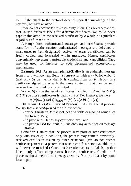
10 PROCESS ALGEBRAS FOR STUDYING SECURITY

16

to c. If the attack to the protocol depends upon the knowledge of the

network, we have an attack.

If we do not account for this possibility in our high-level semantics,

that is, use different labels for different certificates, we could never

capture this attack as the received certificate by e would be equivalent

regardless of i = 0 or i = 1.

Although both authenticated messages and certificates provide

some form of authentication, authenticated messages are delivered at

most once, to their designated receiver, whereas cer-tificates can be

freely copied and forwarded within messages. Hence, certificates

conveniently represent transferable credentials and capabilities. They

may be used, for instance, to code decentralised access-control

mechanisms.

Example 10.2. As an example, a:b⟨Hello⟩ is an authentic message

from a to b with content Hello, a constructor with arity 0, for which b

(and only b) can verify that it is coming from aa{b, Hello} is a

certificate signed by a with the same subterms that can be sent,

received, and verified by any principal.

We let ∅(V ) be the set of certificates included in V and let ∅(V )X

⊆ ∅(V ) be those certifi-cates issued by u ∈ X. For instance, we have

∅(𝑎{0, 𝑏{1}, 𝑐{2}}){𝑎,𝑏} = {𝑏{1}, 𝑎{0, 𝑏{1}, 𝑐{2}}} Definition 10.7 (Well Formed Process). Let P be a local process.

We say that P is well-formed for a 2 Prin when: - any certificate in P that includes a variable or a bound name is of

the form 𝑎{𝑉2}0; - no pattern in P binds any certificate label; and

- no pattern used for input in P matches any authenticated message

from a.

Condition 1 states that the process may produce new certificates

only with issuer a; in addi-tion, the process may contain previously-

received certificates issued by other principals. (We do not restrict

certificate patterns—a pattern that tests a certificate not available to a

will never be matched.) Condition 2 restricts access to labels, so that

labels only affect comparisons between certificates. Condition 3

prevents that authenticated messages sent by P be read back by some

local input.

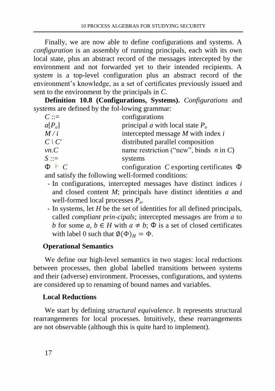
10 PROCESS ALGEBRAS FOR STUDYING SECURITY

17

Finally, we are now able to define configurations and systems. A

configuration is an assembly of running principals, each with its own

local state, plus an abstract record of the messages intercepted by the

environment and not forwarded yet to their intended recipients. A

system is a top-level configuration plus an abstract record of the

environment’s knowledge, as a set of certificates previously issued and

sent to the environment by the principals in C.

Definition 10.8 (Configurations, Systems). Configurations and

systems are defined by the fol-lowing grammar:

C ::= configurations

a[Pa] principal a with local state Pa

M / i intercepted message M with index i

C \ C' distributed parallel composition

vn.C name restriction (“new”, binds n in C)

S ::= systems

Φ C configuration C exporting certificates Φ

and satisfy the following well-formed conditions:

- In configurations, intercepted messages have distinct indices i

and closed content M; principals have distinct identities a and

well-formed local processes Pa.

- In systems, let H be the set of identities for all defined principals,

called compliant prin-cipals; intercepted messages are from a to

b for some a, b ∈ H with a ≠ b; Φ is a set of closed certificates

with label 0 such that ∅(Φ)𝐻 = Φ.

Operational Semantics

We define our high-level semantics in two stages: local reductions

between processes, then global labelled transitions between systems

and their (adverse) environment. Processes, configurations, and systems

are considered up to renaming of bound names and variables.

Local Reductions

We start by defining structural equivalence. It represents structural

rearrangements for local processes. Intuitively, these rearrangements

are not observable (although this is quite hard to implement).

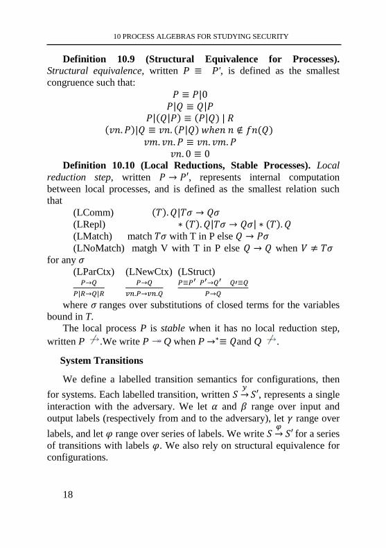
10 PROCESS ALGEBRAS FOR STUDYING SECURITY

18

Definition 10.9 (Structural Equivalence for Processes).

Structural equivalence, written P ≡ P', is defined as the smallest

congruence such that:

𝑃 ≡ 𝑃|0

𝑃|𝑄 ≡ 𝑄|𝑃

𝑃|(𝑄|𝑃) ≡ (𝑃|𝑄) | 𝑅 (𝑣𝑛. 𝑃)|𝑄 ≡ 𝑣𝑛. (𝑃|𝑄) 𝑤ℎ𝑒𝑛 𝑛 ∉ 𝑓𝑛(𝑄)

𝑣𝑚. 𝑣𝑛. 𝑃 ≡ 𝑣𝑛. 𝑣𝑚. 𝑃

𝑣𝑛. 0 ≡ 0 Definition 10.10 (Local Reductions, Stable Processes). Local

reduction step, written 𝑃 → 𝑃′, represents internal computation

between local processes, and is defined as the smallest relation such

that

(LComm) (𝑇). 𝑄|𝑇𝜎 → 𝑄𝜎

(LRepl) ∗ (𝑇). 𝑄|𝑇𝜎 → 𝑄𝜎| ∗ (𝑇). 𝑄

(LMatch) match 𝑇𝜎 with T in P else 𝑄 → 𝑃𝜎

(LNoMatch) matgh V with T in P else 𝑄 → 𝑄 when 𝑉 ≠ 𝑇𝜎

for any 𝜎

(LParCtx) (LNewCtx) (LStruct)

𝑃→𝑄

𝑃|𝑅→𝑄|𝑅

𝑃→𝑄

𝑣𝑛.𝑃→𝑣𝑛.𝑄

𝑃≡𝑃′ 𝑃′→𝑄′ 𝑄′≡𝑄

𝑃→𝑄

where 𝜎 ranges over substitutions of closed terms for the variables

bound in T.

The local process P is stable when it has no local reduction step,

written P .We write P Q when P →∗≡ 𝑄and Q .

System Transitions

We define a labelled transition semantics for configurations, then

for systems. Each labelled transition, written 𝑆𝑦→𝑆′, represents a single

interaction with the adversary. We let 𝛼 and 𝛽 range over input and

output labels (respectively from and to the adversary), let 𝛾 range over

labels, and let 𝜑 range over series of labels. We write 𝑆𝜑→ 𝑆′ for a series

of transitions with labels 𝜑. We also rely on structural equivalence for

configurations.

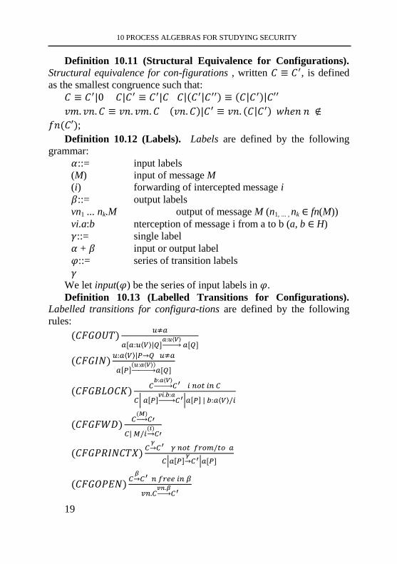
10 PROCESS ALGEBRAS FOR STUDYING SECURITY

19

Definition 10.11 (Structural Equivalence for Configurations).

Structural equivalence for con-figurations , written 𝐶 ≡ 𝐶′, is defined

as the smallest congruence such that:

𝐶 ≡ 𝐶′|0 𝐶|𝐶′ ≡ 𝐶′|𝐶 𝐶|(𝐶′|𝐶′′) ≡ (𝐶|𝐶′)|𝐶′′

𝑣𝑚. 𝑣𝑛. 𝐶 ≡ 𝑣𝑛. 𝑣𝑚. 𝐶 (𝑣𝑛. 𝐶)|𝐶′ ≡ 𝑣𝑛. (𝐶|𝐶′) 𝑤ℎ𝑒𝑛 𝑛 ∉

𝑓𝑛(𝐶′);

Definition 10.12 (Labels). Labels are defined by the following

grammar:

𝛼::= input labels

(M) input of message M

(i) forwarding of intercepted message i

𝛽::= output labels

vn1 ... nk.M output of message M (n1, ... , nk ∈ fn(M))

vi.a:b nterception of message i from a to b (a, b ∈ H)

𝛾::= single label

𝛼 + 𝛽 input or output label

𝜑::= series of transition labels

𝛾

We let input(𝜑) be the series of input labels in 𝜑.

Definition 10.13 (Labelled Transitions for Configurations).

Labelled transitions for configura-tions are defined by the following

rules:

(𝐶𝐹𝐺𝑂𝑈𝑇)𝑢≠𝑎

𝑎[𝑎:𝑢⟨𝑉⟩|𝑄]𝑎:𝑢⟨𝑉⟩→ 𝑎[𝑄]

(𝐶𝐹𝐺𝐼𝑁)𝑢:𝑎⟨𝑉⟩|𝑃→𝑄 𝑢≠𝑎

𝑎[𝑃](𝑢:𝑎⟨𝑉⟩)→ 𝑎[𝑄]

(𝐶𝐹𝐺𝐵𝐿𝑂𝐶𝐾)𝐶𝑏:𝑎⟨𝑉⟩→ 𝐶′ 𝑖 𝑛𝑜𝑡 𝑖𝑛 𝐶

𝐶| 𝑎[𝑃]𝑣𝑖.𝑏:𝑎→ 𝐶′|𝑎[𝑃] | 𝑏:𝑎⟨𝑉⟩/𝑖

(𝐶𝐹𝐺𝐹𝑊𝐷)𝐶(𝑀)→ 𝐶′

𝐶| 𝑀/𝑖(𝑖)→ 𝐶′

(𝐶𝐹𝐺𝑃𝑅𝐼𝑁𝐶𝑇𝑋)𝐶𝛾→𝐶′ 𝛾 𝑛𝑜𝑡 𝑓𝑟𝑜𝑚/𝑡𝑜 𝑎

𝐶|𝑎[𝑃]𝛾→𝐶′|𝑎[𝑃]

(𝐶𝐹𝐺𝑂𝑃𝐸𝑁)𝐶𝛽→𝐶′ 𝑛 𝑓𝑟𝑒𝑒 𝑖𝑛 𝛽

𝑣𝑛.𝐶𝑣𝑛.𝛽→ 𝐶′

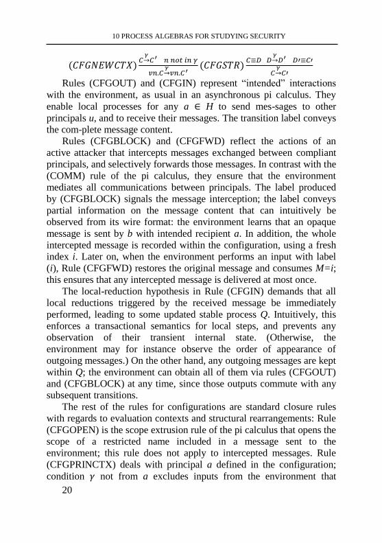
10 PROCESS ALGEBRAS FOR STUDYING SECURITY

20

(𝐶𝐹𝐺𝑁𝐸𝑊𝐶𝑇𝑋)𝐶𝛾→𝐶′ 𝑛 𝑛𝑜𝑡 𝑖𝑛 𝛾

𝑣𝑛.𝐶𝛾→𝑣𝑛.𝐶′

(𝐶𝐹𝐺𝑆𝑇𝑅)𝐶≡𝐷 𝐷

𝛾→𝐷′ 𝐷′≡𝐶′

𝐶𝛾→𝐶′

Rules (CFGOUT) and (CFGIN) represent “intended” interactions

with the environment, as usual in an asynchronous pi calculus. They

enable local processes for any a ∈ H to send mes-sages to other

principals u, and to receive their messages. The transition label conveys

the com-plete message content.

Rules (CFGBLOCK) and (CFGFWD) reflect the actions of an

active attacker that intercepts messages exchanged between compliant

principals, and selectively forwards those messages. In contrast with the

(COMM) rule of the pi calculus, they ensure that the environment

mediates all communications between principals. The label produced

by (CFGBLOCK) signals the message interception; the label conveys

partial information on the message content that can intuitively be

observed from its wire format: the environment learns that an opaque

message is sent by b with intended recipient a. In addition, the whole

intercepted message is recorded within the configuration, using a fresh

index i. Later on, when the environment performs an input with label

(i), Rule (CFGFWD) restores the original message and consumes M=i;

this ensures that any intercepted message is delivered at most once.

The local-reduction hypothesis in Rule (CFGIN) demands that all

local reductions triggered by the received message be immediately

performed, leading to some updated stable process Q. Intuitively, this

enforces a transactional semantics for local steps, and prevents any

observation of their transient internal state. (Otherwise, the

environment may for instance observe the order of appearance of

outgoing messages.) On the other hand, any outgoing messages are kept

within Q; the environment can obtain all of them via rules (CFGOUT)

and (CFGBLOCK) at any time, since those outputs commute with any

subsequent transitions.

The rest of the rules for configurations are standard closure rules

with regards to evaluation contexts and structural rearrangements: Rule

(CFGOPEN) is the scope extrusion rule of the pi calculus that opens the

scope of a restricted name included in a message sent to the

environment; this rule does not apply to intercepted messages. Rule

(CFGPRINCTX) deals with principal a defined in the configuration;

condition 𝛾 not from a excludes inputs from the environment that

10 PROCESS ALGEBRAS FOR STUDYING SECURITY

21

would forge a message from a, whereas condition 𝛾 not to a excludes

outputs that may be transformed by Rule (CFGBLOCK).

Finally, we have a pair of top level rules that deal with the attacker

knowledge:

Definition 10.14 (Labelled Transitions for Systems). Labelled

transitions for systems are de-fined by the following rules:

(𝑆𝑌𝑆𝑂𝑈𝑇)𝐶𝛽→𝐶′

Φ 𝐶𝛽→ Φ∪ ∅(β)HC′

(𝑆𝑌𝑆𝐼𝑁)𝐶𝑎→𝐶′ ∅(𝑎)𝐻⊆𝑀(Φ)

Φ Ca→Φ C′

where H is the set of principals defined in C and 𝑀(Φ) ={𝑎{𝑉}𝑙: 𝑎{𝑉}0 ∈ Φ} is the set of certificates the attacker might produce

from Φ (see Appendix A for the motivation for this rule).

Rule (SYSOUT) filters every output 𝛽 and adds to Φ the

certificates included in 𝛽. Rule (SYSIN) filters every input a, and

checks that the certificates included in a can be produce from the

certificates in Φ.

Our main results are expressed using normal transitions between

systems.

Definition 10.15 (Stable Systems, Normal Transitions). We say

that the system S is stable when all local processes of S are stable and S

has no output transition. (Informally, S is waiting for any input from the

environment.)

We say that a series of transitions 𝑆𝜑→𝑆′

is normal when every

input transition is followed by a maximal series of output transitions

leading to a stable system, that is, 𝜑 = 𝜑1𝜑2…𝜑𝑛 where 𝜑𝑖 = 𝑎𝑖𝛽�̃� for

𝑖 = 1. . 𝑛, and 𝑆 = 𝑆0𝜑1→ 𝑆1

𝜑2→ 𝑆2…

𝜑𝑛→ 𝑆𝑛 = 𝑆

′ for some stable systems

𝑆0, … , 𝑆𝑛.

Intuitively normality states that each principals outputs all his

messages and stays idle until he receives a new input.

Compositionality

By design, our semantics is compositional, as its rules are

inductively defined on the structure of configurations. For instance, we

obtain that interactions with a principal that is implicitly controlled by

the environment are at least as expressive as those with any principal

explicited within the system.

10 PROCESS ALGEBRAS FOR STUDYING SECURITY

22

If we have 𝐶 |𝑎[𝑃]𝑎→ 𝐶′| [𝑃], then we also have 𝐶𝑜

𝛽→ 𝐶′0 , where

𝐶𝑜 and 𝐶′0 are obtained from C and C', respectively, by erasing the

state associated with a: any intercepted messages M / i from a or to a;

and any certificate in Φ issued by a. This compositional property yields

useful congruence properties for observational equivalence on

configurations.

An Abstract Machine for Local Reductions

In preparation to the description of a concrete machine Ma that

executes a’s local process Pa, we derive a simple algorithm for local

reductions. In contrast with our non-deterministic reduction semantics,

the algorithm relies on partial normal forms instead of structural

equivalence, and it carefully controls the creation of fresh names (to be

implemented as random-number generation); it also relies on an explicit

scheduler and is otherwise deterministic.

A process P is in normal form for a when it is a closed well-formed

process such that every subprocess of the form match V with T in Q

else Q' or vn.Q appears only under an input or a replicated input—

intuitively, all name creations and matchings are guarded. Let P be in

normal form for a. Up to the structural laws for parallel composition,

𝑃 ≡ 𝑀| 𝐿 |𝐺 where M is a parallel composition of messages sent to

other principals, L is a parallel composition of other (local) messages,

and G is a parallel composition of inputs and replicated inputs.

Concretely, we may represent P as a triple of multisets for M, L, and G.

A scheduler is a deterministic algorithm on (L,G) that selects an

instance of Rule (LCOMM) or (LREPL) for an output of L and an input

(or replicated input) of G, if any, and otherwise reports completion. The

reduction algorithm repeatedly calls the scheduler, performs the

selected reduction step, then normalises the resulting process by

applying Rules (LMATCH) and (LNOMATCH) and lifting name

restrictions to the top level (possibly after a renaming). This yields a

local pro-cess of the form v�̃�:(M' | L' | G') where �̃� collect all new

name restrictions in evaluation context. By induction on the length of

the derivation, one easily check that P → Q if and only if, for local

process is in normal form.

10 PROCESS ALGEBRAS FOR STUDYING SECURITY

23

A configuration is in normal form when all restrictions are grouped

at top-level and every local process is in normal form. Our local

reduction strategy can be extended to configurations in normal forms

as follows: we perform local reductions as detailed above, then lift any

resulting restrictions to the top level of the configuration up to

structural equivalence (using a[v�̃�:P' ]≡ 𝑣�̃� .a[P'])

10.3 High-Level Equivalences and Safety

Now that we have defined labelled transitions that capture our

attacker model and implementation constraints, we can apply standard

definitions and proof techniques from concurrency theory to reason

about systems. Our computational soundness results are useful (and

non-trivial) inasmuch as transitions are simpler and more abstract than

low-level adversaries. In addition to trace properties (used, for instance,

to express authentication properties as correspondences between

transitions), we consider equivalences between systems.

Intuitively, two systems are equivalent when their environment

observes the same transitions. Looking at immediate observations, we

say that two systems 𝑆1 and 𝑆2 have the same labels when, if 𝑆1𝛾→𝑆2

for some 𝑆1′ (and the name exported by are not free in 𝑆2), then

𝑆2𝛾→𝑆2

′ for some 𝑆2

′ , and vice versa. More generally, bisimilarity

demands that this remains the case after matching transitions:

Definition 10.16 (Bisimilarity). The relation R on systems is a

labelled simulation when, for all 𝑆1 𝑅 𝑆2, if 𝑆1𝛾→𝑆1

′ (and the names

exported by 𝛾 are not free in 𝑆2) then 𝑆2𝛾→𝑆2

′ and 𝑆1′ R 𝑆2

′ . Labelled

bisimilarity, written ≅, is the largest symmetric labelled simulation.

In particular, if Φ C ≅ Φ′ C′ then C and C' define the same

principals, intercepted-message indices, and exported certificates (

M(Φ) = M(Φ′)). We also easily verify some congruence properties: our equivalence

is preserved by addition of principals, deletion of intercepted messages,

and deletion of certificates.

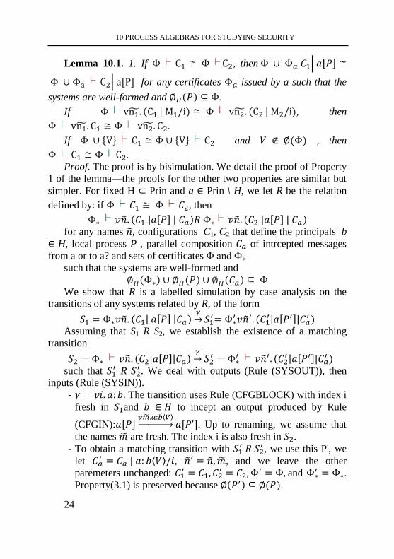
10 PROCESS ALGEBRAS FOR STUDYING SECURITY

24

Lemma 10.1. 1. If Φ C1 ≅ Φ C2, then Φ ∪ Φ𝑎 𝐶1| 𝑎[𝑃] ≅

Φ ∪ Φa C2| a[P] for any certificates Φ𝑎 issued by a such that the

systems are well-formed and ∅𝐻(𝑃) ⊆ Φ.

If Φ vn1̃. (C1 | M1/i) ≅ Φ vn2̃. (C2 | M2/i), then

Φ vn1̃. C1 ≅ Φ vn2̃. C2.

If Φ ∪ {V} C1 ≅ Φ∪ {V} C2 and 𝑉 ∉ ∅(Φ) , then

Φ C1 ≅ Φ C2.

Proof. The proof is by bisimulation. We detail the proof of Property

1 of the lemma—the proofs for the other two properties are similar but

simpler. For fixed H ⊂ Prin and a ∈ Prin \ H, we let R be the relation

defined by: if Φ 𝐶1 ≅ Φ 𝐶2, then

Φ∗ 𝑣�̃�. (𝐶1 |𝑎[𝑃] | 𝐶𝑎)𝑅 Φ∗ 𝑣�̃�. (𝐶2 |𝑎[𝑃] | 𝐶𝑎) for any names �̃�, configurations C1, C2 that define the principals b

∈ H, local process P , parallel composition 𝐶𝑎 of intrcepted messages

from a or to a? and sets of certificates Φ and Φ∗ such that the systems are well-formed and

∅𝐻(Φ∗) ∪ ∅𝐻(𝑃) ∪ ∅𝐻(𝐶𝑎) ⊆ Φ We show that R is a labelled simulation by case analysis on the

transitions of any systems related by R, of the form

𝑆1 = Φ∗𝑣�̃�. (𝐶1| 𝑎[𝑃] |𝐶𝑎)𝛾→𝑆1

′= Φ∗′𝑣�̃�′. (𝐶1

′|𝑎[𝑃′]|𝐶𝑎′ )

Assuming that S1 R S2, we establish the existence of a matching

transition

𝑆2 = Φ∗ 𝑣�̃�. (𝐶2|𝑎[𝑃]|𝐶𝑎)𝛾→ 𝑆2

′ = Φ∗′ 𝑣�̃�′. (𝐶2

′ |𝑎[𝑃′]|𝐶𝑎′ )

such that 𝑆1′ R 𝑆2

′ . We deal with outputs (Rule (SYSOUT)), then

inputs (Rule (SYSIN)).

- 𝛾 = 𝑣𝑖. 𝑎: 𝑏. The transition uses Rule (CFGBLOCK) with index i

fresh in 𝑆1and 𝑏 ∈ 𝐻 to incept an output produced by Rule

(CFGIN):𝑎[𝑃]𝑣�̃�.𝑎:𝑏⟨𝑉⟩→ 𝑎[𝑃′]. Up to renaming, we assume that

the names �̃� are fresh. The index i is also fresh in 𝑆2.

- To obtain a matching transition with 𝑆1′ 𝑅 𝑆2

′ , we use this P', we

let 𝐶𝑎′ = 𝐶𝑎 | 𝑎: 𝑏⟨𝑉⟩/𝑖, �̃�

′ = �̃�, �̃�, and we leave the other

paremeters unchanged: 𝐶1′ = 𝐶1, 𝐶2

′ = 𝐶2, Φ′ = Φ, and Φ∗

′ = Φ∗. Property(3.1) is preserved because ∅(𝑃′) ⊆ ∅(𝑃).

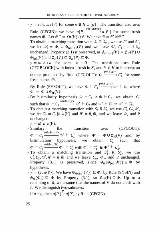
10 PROCESS ALGEBRAS FOR STUDYING SECURITY

25

- 𝛾 = 𝑣�̃�. 𝑎: 𝑒⟨𝑉⟩ for some e ∉ 𝐻 ∪ {𝑎} . The transition also uses

Rule (CFGIN): we have 𝑎[𝑃]𝑣�̃�′.𝑎:𝑏⟨𝑉⟩→ 𝑎[𝑃′] for some fresh

names �̃�′. Let �̃�′′ = 𝑓𝑛(𝑉) ∩ �̃�. We have �̃� = �̃�′ �̃�′′. - To obtain a matching transition with 𝑆1

′ R 𝑆2′ , we use 𝑃′ and �̃�′,

we let Φ∗′ = Φ∗ ∪ ∅𝐻∪{𝑎}(𝑉) and we leave Φ', 𝐶1 , and 𝐶2

unchanged. Property (3.1) is preserved, as ∅𝐻∪{𝑎}(𝑉) = ∅𝐻(𝑉) ∪

∅{𝑎}(𝑉) and ∅𝐻(𝑉) ⊆ ∅𝐻(𝑃) ⊆ Φ.

- 𝛾 = 𝑣𝑖. 𝑏 ∶ 𝑎 for some 𝑏 ∈ 𝐻. The transition uses Rule

(CFGBLOCK) with index i fresh in 𝑆1 and 𝑏 ∈ 𝐻 to intercept an

output produced by Rule (CFGOUT): 𝐶1𝑣�̃�𝑏:𝑎⟨𝑉⟩→ 𝐶1

′ for some

fresh names �̃�.

- By Rule (SYSOUT), we have Φ 𝐶1𝑣�̃�𝑏:𝑎⟨𝑉⟩→ Φ′ 𝐶1

′ where

Φ′ = Φ ∪ ∅H(V).

- By bisimilarity hypothesis Φ C1 ≅ Φ C2, we obtain 𝐶1′

such that Φ C2𝑣�̃�𝑏:𝑎⟨𝑉⟩→ Φ′ C2

′ and Φ′ C1′ ≅ Φ′ C2

′ .

- To obtain a matching transition with 𝑆1′ 𝑅 𝑆2

′ , we use 𝐶1′ , 𝐶2

′ , Φ′, we let 𝐶𝑎

′ = 𝐶𝑎|𝑏: 𝑎⟨𝑉⟩ and �̃�′ = �̃�, �̃�, and we leave Φ∗ and P

unchanged.

- 𝛾 = �̃�. 𝑏: 𝑒⟨𝑉⟩. - Similary, the transition uses (CFGOUT):

Φ 𝐶1𝑣�̃�′𝑏:𝑎⟨𝑉⟩→ Φ′ 𝐶1

′ where Φ′ = Φ ∪ ∅H(V) and, by

bisimulation hypothesis, we obtain 𝐶2′ such that

Φ 𝐶2𝑣�̃�𝑏:𝑎⟨𝑀⟩→ Φ′ 𝐶2

′ with Φ′ 𝐶1′ ≅ Φ ′ 𝐶2

′ .

- To obtain a matching transition and 𝑆1′ R 𝑆2

′ , we use

𝐶1′ , 𝐶2

′ , Φ′, �̃�′ = �̃�, �̃� and we leave 𝐶𝑎, Φ∗, and P unchanged.

Property (3.1) is preserved, since ∅𝐻(∅{𝑎}(𝑀)) ⊆ Φ by

hypothesis.

- 𝛾 = (𝑒: 𝑢⟨𝑉⟩). We have ∅𝐻∪{𝑎}(𝑉)) ⊆ Φ∗ by Rule (SYSIN) and

∅𝐻(Φ∗) ⊆ Φ by Property (3.1), so ∅𝐻(𝑉) ⊆ Φ. Up to a

renaming of �̃�, we assume that the names of V do not clash with

�̃�. We distinguish two subcases:

- if u = a, then a[P ]𝛾→ a[P'] by Rule (CFGIN).

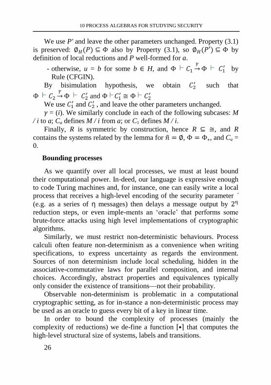
10 PROCESS ALGEBRAS FOR STUDYING SECURITY

26

We use P' and leave the other parameters unchanged. Property (3.1)

is preserved: ∅𝐻(𝑃) ⊆ Φ also by Property (3.1), so ∅𝐻(𝑃′) ⊆ Φ by

definition of local reductions and P well-formed for a.

- otherwise, u = b for some b ∈ H, and Φ 𝐶1𝛾→Φ 𝐶1

′ by

Rule (CFGIN).

By bisimulation hypothesis, we obtain 𝐶2′ such that

Φ 𝐶2𝛾→Φ 𝐶2

′ and Φ 𝐶1′ ≅ Φ 𝐶2

′

We use 𝐶1′ and 𝐶2

′ , and leave the other parameters unchanged.

𝛾 = (i). We similarly conclude in each of the following subcases: M

/ i to a; Ca defines M / i from a; or C1 defines M / i.

Finally, R is symmetric by construction, hence R ⊆ ≅, and R

contains the systems related by the lemma for �̃� = ∅, Φ = Φ∗, and Ca =

0.

Bounding processes

As we quantify over all local processes, we must at least bound

their computational power. In-deed, our language is expressive enough

to code Turing machines and, for instance, one can easily write a local

process that receives a high-level encoding of the security parameter ´

(e.g. as a series of η messages) then delays a message output by 2η

reduction steps, or even imple-ments an ‘oracle’ that performs some

brute-force attacks using high level implementations of cryptographic

algorithms.

Similarly, we must restrict non-deterministic behaviours. Process

calculi often feature non-determinism as a convenience when writing

specifications, to express uncertainty as regards the environment.

Sources of non determinism include local scheduling, hidden in the

associative-commutative laws for parallel composition, and internal

choices. Accordingly, abstract properties and equivalences typically

only consider the existence of transitions—not their probability. Observable non-determinism is problematic in a computational

cryptographic setting, as for in-stance a non-deterministic process may

be used as an oracle to guess every bit of a key in linear time.

In order to bound the complexity of processes (mainly the

complexity of reductions) we de-fine a function ⌈•⌉ that computes the

high-level structural size of systems, labels and transitions.

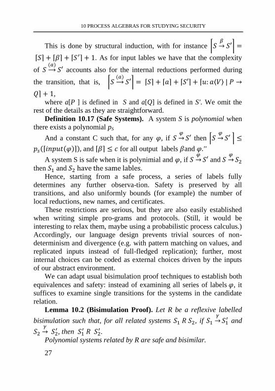
10 PROCESS ALGEBRAS FOR STUDYING SECURITY

27

This is done by structural induction, with for instance ⌈𝑆𝛽→ 𝑆′⌉ =

⌈𝑆⌉ + ⌈𝛽⌉ + ⌈𝑆′⌉ + 1. As for input lables we have that the complexity

of 𝑆(𝑎)→ 𝑆′ accounts also for the internal reductions performed during

the transition, that is, ⌈𝑆(𝑎)→ 𝑆′⌉ = ⌈𝑆⌉ + ⌈𝑎⌉ + ⌈𝑆′⌉ + ⌈𝑢: 𝑎⟨𝑉⟩ | 𝑃 →

𝑄⌉ + 1,

where a[P ] is defined in S and a[Q] is defined in S'. We omit the

rest of the details as they are straightforward.

Definition 10.17 (Safe Systems). A system S is polynomial when

there exists a polynomial pS

And a constant C such that, for any 𝜑, if 𝑆𝜑→𝑆′ then ⌈𝑆

𝜑→𝑆′ ⌉ ≤

𝑝𝑠(⌈𝑖𝑛𝑝𝑢𝑡(𝜑)⌉), and ⌈𝛽⌉ ≤ 𝑐 for all output labels 𝛽and 𝜑.''

A system S is safe when it is polynimial and 𝜑, if 𝑆𝜑→𝑆′ and 𝑆

𝜑→𝑆2

then 𝑆1 and 𝑆2 have the same lables. Hence, starting from a safe process, a series of labels fully

determines any further observa-tion. Safety is preserved by all

transitions, and also uniformly bounds (for example) the number of

local reductions, new names, and certificates.

These restrictions are serious, but they are also easily established

when writing simple pro-grams and protocols. (Still, it would be

interesting to relax them, maybe using a probabilistic process calculus.)

Accordingly, our language design prevents trivial sources of non-

determinism and divergence (e.g. with pattern matching on values, and

replicated inputs instead of full-fledged replication); further, most

internal choices can be coded as external choices driven by the inputs

of our abstract environment.

We can adapt usual bisimulation proof techniques to establish both

equivalences and safety: instead of examining all series of labels 𝜑, it

suffices to examine single transitions for the systems in the candidate

relation.

Lemma 10.2 (Bisimulation Proof). Let R be a reflexive labelled

bisimulation such that, for all related systems 𝑆1 𝑅 𝑆2, if 𝑆1𝛾→𝑆1

′ and

𝑆2𝛾→ 𝑆2

′ , then 𝑆1′ 𝑅 𝑆2

′ .

Polynomial systems related by R are safe and bisimilar.

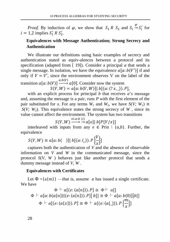
10 PROCESS ALGEBRAS FOR STUDYING SECURITY

28

Proof. By induction of 𝜑, we show that 𝑆1 𝑅 𝑆2 and 𝑆𝑖𝜑→𝑆𝑖

′ for

𝑖 = 1,2 implies 𝑆1′ 𝑅 𝑆2

′ .

Equivalences with Message Authentication; Strong Secrecy and

Authentication

We illustrate our definitions using basic examples of secrecy and

authentication stated as equiv-alences between a protocol and its

specification (adapted from [ 19]). Consider a principal a that sends a

single message. In isolation, we have the equivalence 𝑎[𝑎: 𝑏⟨𝑉′⟩] if and

only if 𝑉 = 𝑉′, since the environment observes V on the label of the

transition 𝑎[𝑎: 𝑏⟨𝑉⟩]𝑎:𝑏⟨𝑉⟩→ 𝑎[0]. Consider now the system

𝑆(𝑉,𝑊) = 𝑎[𝑎: 𝑏⟨𝑉,𝑊⟩]| 𝑏[(𝑎: ⟨? 𝑥, _⟩). 𝑃], with an explicit process for principal b that receives a’s message

and, assuming the message is a pair, runs P with the first element of the

pair substituted for x. For any terms W1 and W2, we have S(V; W1) ≅ S(V; W2). This equivalence states the strong secrecy of W , since its

value cannot affect the environment. The system has two transitions

𝑆(𝑉,𝑊)𝑣𝑖.𝑎:𝑏→

(𝑖)→ 𝑎[𝑜]| 𝑏[𝑃{𝑉/𝑥}]

interleaved with inputs from any e ∈ Prin \ {a,b}. Further, the

equivalence

𝑆(𝑉,𝑊) ≅ 𝑎[𝑎: 𝑏⟨ ⟩]| 𝑏[(𝑎: ⟨_⟩). 𝑃 {𝑉

𝑥}]

captures both the authentication of V and the absence of observable

information on V and W in the communicated message, since the

protocol S(V, W ) behaves just like another protocol that sends a

dummy message instead of V, W .

Equivalences with Certificates

Let Φ ={a{m}} —that is, assume a has issued a single certificate.

We have

Φ 𝑎[(𝑒: ⟨𝑎{𝑛}⟩). 𝑃] ≅ Φ 𝑎[]

Φ 𝑎[𝑎: 𝑏⟨𝑎{𝑛}⟩|(𝑒: ⟨𝑎{𝑛}⟩). 𝑃]| 𝑏[] ≅ Φ 𝑎[𝑎: 𝑏⟨0⟩]|𝑏[]

Φ 𝑎[(𝑒: ⟨𝑎{𝑥}⟩). 𝑃] ≅ Φ 𝑎{(𝑒: ⟨𝑎{_}⟩). 𝑃 {𝑚

𝑥}]

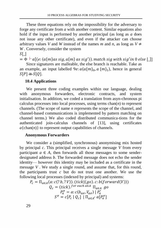
10 PROCESS ALGEBRAS FOR STUDYING SECURITY

29

These three equations rely on the impossibility for the adversary to

forge any certificate from a with another content. Similar equations also

hold if the input is performed by another principal (as long as a does

not issue any other certificate), and even if the attacker can choose

arbitrary values V and W instead of the names m and n, as long as V ≠

W . Conversely, consider the system

𝑆[_]

= Φ 𝑎[(𝑒: ⟨𝑎{𝑚}𝑎𝑠 𝑠𝑖𝑔, 𝑎{𝑚} 𝑎𝑠 𝑠𝑖𝑔′⟩).𝑚𝑎𝑡𝑐ℎ 𝑠𝑖𝑔 𝑤𝑖𝑡ℎ 𝑠𝑖𝑔′𝑖𝑛 0 𝑒𝑙𝑠𝑒 [_]] Since signatures are malleable, the else branch is reachable. Take as

an example, an input labelled 9𝑒: 𝑎⟨𝑎{𝑚}0, 𝑎 {𝑚}1⟩, hence in general

𝑆[𝑃] ≅ 𝑆[𝑄].

10.4 Applications

We present three coding examples within our language, dealing

with anonymous forwarders, electronic contracts, and system

initialisation. In addition, we coded a translation from asyn-chronous pi

calculus processes into local processes, using terms chan(n) to represent

channels. (The scope of name n represents the scope of the channel, and

channel-based communications is implemented by pattern matching on

channel terms.) We also coded distributed communica-tions for the

authenticated join-calculus channels of [13], using certificates

a{chan(n)} to represent output capabilities of channels.

Anonymous Forwarders

We consider a (simplified, synchronous) anonymising mix hosted

by principal c. This principal receives a single message V from every

participant a ∈ A, then forwards all those messages to some sender-

designated address b. The forwarded message does not echo the sender

identity— however this identity may be included as a certificate in the

message V . We study a single round, and assume that, for this round,

the participants trust c but do not trust one another. We use the

following local processes (indexed by principal) and systems:

𝑃𝑐 = П𝑎∈𝐴(𝑎: 𝑐⟨? 𝑏, ? 𝑉⟩). (𝑡𝑖𝑐𝑘|(𝑔𝑜). 𝑐: 𝑏⟨𝑓𝑜𝑟𝑤𝑎𝑟𝑑(𝑉)⟩) 𝑄𝑐 = (𝑡𝑖𝑐𝑘).

𝑓𝑜𝑟 𝑒𝑎𝑐ℎ 𝑎∈𝐴 П𝑎∈𝐴 𝑔𝑜 𝑃𝑎𝜎 = 𝑎: 𝑐⟨𝑏𝑎𝜎 , 𝑉𝑎𝜎⟩ | 𝑃𝑎

′

𝑆𝜎 = 𝑐[𝑃𝑐 | 𝑄𝑐] | П𝑎∈𝐴′ 𝑎[𝑃𝑎𝜎]

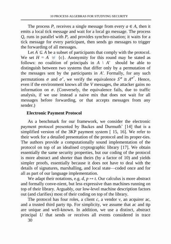
10 PROCESS ALGEBRAS FOR STUDYING SECURITY

30

The process Pc receives a single message from every a ∈ A, then it

emits a local tick message and wait for a local go message. The process

Qc runs in parallel with Pc and provides synchro-nisation; it waits for a

tick message for every participant, then sends go messages to trigger

the forwarding of all messages.

Let A' ⊆ A be a subset of participants that comply with the protocol.

We set H = A'

{c}. Anonymity for this round may be stated as

follows: no coalition of principals in A \ A' should be able to

distinguish between two systems that differ only by a permutation of

the messages sent by the participants in A'. Formally, for any such

permutations 𝜎 and 𝜎′, we verify the equivalence 𝑆𝜎 ≅ 𝐴𝜎′. Hence,

even if the environment knows all the V messages, the attacker gains no

information on 𝜎. (Conversely, the equivalence fails, due to traffic

analysis, if we use instead a naive mix that does not wait for all

messages before forwarding, or that accepts messages from any

sender.)

Electronic Payment Protocol

As a benchmark for our framework, we consider the electronic

payment protocol presented by Backes and Durmuth¨ [14] that is a

simplified version of the 3KP payment system [ 15, 16]. We refer to

their work for a detailed presentation of the protocol and its proper-ties.

The authors provide a computationally sound implementation of the

protocol on top of an idealised cryptographic library [17]. We obtain

essentially the same security properties, but our coding of the protocol

is more abstract and shorter than theirs (by a factor of 10) and yields

simpler proofs, essentially because it does not have to deal with the

details of signatures, marshalling, and local state—coded once and for

all as part of our language implementation.

We adapt their notations, e.g. d, p ↦ t. Our calculus is more abstract

and formally conve-nient, but less expressive than machines running on

top of their library. Arguably, our low-level machine description factors

out (and clarifies) most of their coding on top of the library.

The protocol has four roles, a client c, a vendor v, an acquirer ac,

and a trusted third party ttp. For simplicity, we assume that ac and ttp

are unique and well-known. In addition, we use a distinct, abstract

principal U that sends or receives all events considered in trace

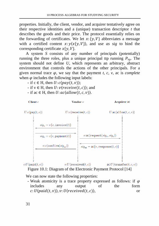
10 PROCESS ALGEBRAS FOR STUDYING SECURITY

31

properties. Initially, the client, vendor, and acquirer tentatively agree on

their respective identities and a (unique) transaction descriptor t that

describes the goods and their price. The protocol essentially relies on

the forwarding of certificates. We let 𝑥: {𝑦, 𝑉} abbreviates a message

with a certified content 𝑥: 𝑦⟨𝑥{𝑦, 𝑉}⟩, and use as sig to bind the

corresponding certificate 𝑥{𝑦, 𝑉}. A system S consists of any number of principals (potentially)

running the three roles, plus a unique principal ttp running Pttp. The

system should not define U, which represents an arbitrary, abstract

environment that controls the actions of the other principals. For a

given normal trace 𝜑, we say that the payment t, c, v, ac is complete

when 𝜑 includes the following input labels:

- if c ∈ H, then 𝑈: 𝑐⟨𝑝𝑎𝑦(𝑡, 𝑣)⟩; - if v ∈ H, then 𝑈: 𝑣⟨𝑟𝑒𝑐𝑒𝑖𝑣𝑒(𝑡, 𝑐)⟩; and

- if ac ∈ H, then 𝑈: 𝑎𝑐⟨𝑎𝑙𝑙𝑜𝑤(𝑡, 𝑐, 𝑣)⟩.

Figure 10.1: Diagram of the Electronic Payment Protocol [14]

We can now state the following properties:

- Weak atomicity is a trace property expressed as follows: if 𝜑

includes any output of the form

𝑐: 𝑈⟨𝑝𝑎𝑖𝑑(𝑡, 𝑣)⟩, 𝑣: 𝑈⟨𝑟𝑒𝑐𝑒𝑖𝑣𝑒𝑑(𝑡, 𝑐)⟩, or

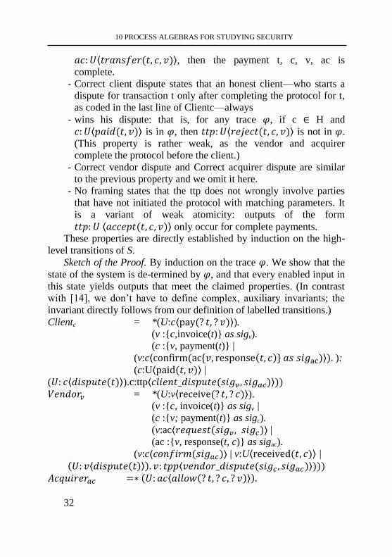
10 PROCESS ALGEBRAS FOR STUDYING SECURITY

32

𝑎𝑐:𝑈⟨𝑡𝑟𝑎𝑛𝑠𝑓𝑒𝑟(𝑡, 𝑐, 𝑣)⟩, then the payment t, c, v, ac is

complete.

- Correct client dispute states that an honest client—who starts a

dispute for transaction t only after completing the protocol for t,

as coded in the last line of Clientc—always

- wins his dispute: that is, for any trace 𝜑, if c ∈ H and

𝑐: 𝑈⟨𝑝𝑎𝑖𝑑(𝑡, 𝑣)⟩ is in 𝜑, then 𝑡𝑡𝑝: 𝑈⟨𝑟𝑒𝑗𝑒𝑐𝑡(𝑡, 𝑐, 𝑣)⟩ is not in 𝜑.

(This property is rather weak, as the vendor and acquirer

complete the protocol before the client.)

- Correct vendor dispute and Correct acquirer dispute are similar

to the previous property and we omit it here.

- No framing states that the ttp does not wrongly involve parties

that have not initiated the protocol with matching parameters. It

is a variant of weak atomicity: outputs of the form

𝑡𝑡𝑝: 𝑈 ⟨𝑎𝑐𝑐𝑒𝑝𝑡(𝑡, 𝑐, 𝑣)⟩ only occur for complete payments.

These properties are directly established by induction on the high-

level transitions of S.

Sketch of the Proof. By induction on the trace 𝜑. We show that the

state of the system is de-termined by 𝜑, and that every enabled input in

this state yields outputs that meet the claimed properties. (In contrast

with [14], we don’t have to define complex, auxiliary invariants; the

invariant directly follows from our definition of labelled transitions.)

Clientc = *(U:𝑐⟨pay(? 𝑡, ? 𝑣)⟩). (v :{c,invoice(t)} as sigv).

(c :{v, payment(t)} |

(v:c⟨confirm(ac{𝑣, response(𝑡, 𝑐)} 𝑎𝑠 𝑠𝑖𝑔ac)⟩). ):

(c:U⟨paid(𝑡, 𝑣)⟩ | (𝑈: 𝑐⟨𝑑𝑖𝑠𝑝𝑢𝑡𝑒(𝑡)⟩).c:ttp⟨𝑐𝑙𝑖𝑒𝑛𝑡_𝑑𝑖𝑠𝑝𝑢𝑡𝑒(𝑠𝑖𝑔𝑣 , 𝑠𝑖𝑔𝑎𝑐)⟩)) 𝑉𝑒𝑛𝑑𝑜𝑟𝑣 = *(U:v⟨receive(? 𝑡, ? 𝑐)⟩). (v :{c, invoice(t)} as sigv |

(c :{v; payment(t)} as sigc).

(v:ac⟨𝑟𝑒𝑞𝑢𝑒𝑠𝑡(𝑠𝑖𝑔𝑣 , 𝑠𝑖𝑔𝑐)⟩ | (ac :{v, response(t, c)} as sigac).

(v:c⟨𝑐𝑜𝑛𝑓𝑖𝑟𝑚(𝑠𝑖𝑔𝑎𝑐)⟩ | v:U⟨received(𝑡, 𝑐)⟩ | (𝑈: 𝑣⟨𝑑𝑖𝑠𝑝𝑢𝑡𝑒(𝑡)⟩). 𝑣: 𝑡𝑝𝑝⟨𝑣𝑒𝑛𝑑𝑜𝑟_𝑑𝑖𝑠𝑝𝑢𝑡𝑒(𝑠𝑖𝑔𝑐 , 𝑠𝑖𝑔𝑎𝑐)⟩)))

𝐴𝑐𝑞𝑢𝑖𝑟𝑒𝑟𝑎𝑐 =∗ (𝑈: 𝑎𝑐⟨𝑎𝑙𝑙𝑜𝑤(? 𝑡, ? 𝑐, ? 𝑣)⟩).

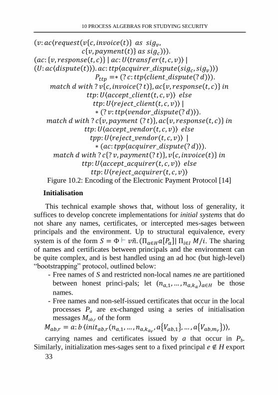
10 PROCESS ALGEBRAS FOR STUDYING SECURITY

33

(𝑣: 𝑎𝑐⟨𝑟𝑒𝑞𝑢𝑒𝑠𝑡(𝑣{𝑐, 𝑖𝑛𝑣𝑜𝑖𝑐𝑒(𝑡)} 𝑎𝑠 𝑠𝑖𝑔𝑣,𝑐{𝑣, 𝑝𝑎𝑦𝑚𝑒𝑛𝑡(𝑡)} 𝑎𝑠 𝑠𝑖𝑔𝑐)⟩).

(𝑎𝑐: {𝑣, 𝑟𝑒𝑠𝑝𝑜𝑛𝑠𝑒(𝑡, 𝑐)} | 𝑎𝑐: 𝑈⟨𝑡𝑟𝑎𝑛𝑠𝑓𝑒𝑟(𝑡, 𝑐, 𝑣)⟩ | (𝑈: 𝑎𝑐⟨𝑑𝑖𝑠𝑝𝑢𝑡𝑒(𝑡)⟩). 𝑎𝑐: 𝑡𝑡𝑝⟨𝑎𝑐𝑞𝑢𝑖𝑟𝑒𝑟_𝑑𝑖𝑠𝑝𝑢𝑡𝑒(𝑠𝑖𝑔𝑐 , 𝑠𝑖𝑔𝑣)⟩)

𝑃𝑡𝑡𝑝 =∗ (? 𝑐: 𝑡𝑡𝑝⟨𝑐𝑙𝑖𝑒𝑛𝑡_𝑑𝑖𝑠𝑝𝑢𝑡𝑒(? 𝑑)⟩).

𝑚𝑎𝑡𝑐ℎ 𝑑 𝑤𝑖𝑡ℎ ? 𝑣{𝑐, 𝑖𝑛𝑣𝑜𝑖𝑐𝑒(? 𝑡)}, 𝑎𝑐{𝑣, 𝑟𝑒𝑠𝑝𝑜𝑛𝑠𝑒(𝑡, 𝑐)} 𝑖𝑛

𝑡𝑡𝑝: 𝑈⟨𝑎𝑐𝑐𝑒𝑝𝑡_𝑐𝑙𝑖𝑒𝑛𝑡(𝑡, 𝑐, 𝑣)⟩ 𝑒𝑙𝑠𝑒 𝑡𝑡𝑝: 𝑈⟨𝑟𝑒𝑗𝑒𝑐𝑡_𝑐𝑙𝑖𝑒𝑛𝑡(𝑡, 𝑐, 𝑣)⟩ | ∗ (? 𝑣: 𝑡𝑡𝑝⟨𝑣𝑒𝑛𝑑𝑜𝑟_𝑑𝑖𝑠𝑝𝑢𝑡𝑒(? 𝑑)⟩).

𝑚𝑎𝑡𝑐ℎ 𝑑 𝑤𝑖𝑡ℎ ? 𝑐{𝑣, 𝑝𝑎𝑦𝑚𝑒𝑛𝑡 (? 𝑡)}, 𝑎𝑐{𝑣, 𝑟𝑒𝑠𝑝𝑜𝑛𝑠𝑒(𝑡, 𝑐)} 𝑖𝑛

𝑡𝑡𝑝: 𝑈⟨𝑎𝑐𝑐𝑒𝑝𝑡_𝑣𝑒𝑛𝑑𝑜𝑟(𝑡, 𝑐, 𝑣)⟩ 𝑒𝑙𝑠𝑒

𝑡𝑝𝑝:𝑈⟨𝑟𝑒𝑗𝑒𝑐𝑡_𝑣𝑒𝑛𝑑𝑜𝑟(𝑡, 𝑐, 𝑣)⟩ | ∗ (𝑎𝑐: 𝑡𝑝𝑝⟨𝑎𝑐𝑞𝑢𝑖𝑟𝑒𝑟_𝑑𝑖𝑠𝑝𝑢𝑡𝑒(? 𝑑)⟩).

𝑚𝑎𝑡𝑐ℎ 𝑑 𝑤𝑖𝑡ℎ ? 𝑐{? 𝑣, 𝑝𝑎𝑦𝑚𝑒𝑛𝑡(? 𝑡)}, 𝑣{𝑐, 𝑖𝑛𝑣𝑜𝑖𝑐𝑒(𝑡)} 𝑖𝑛

𝑡𝑡𝑝: 𝑈⟨𝑎𝑐𝑐𝑒𝑝𝑡_𝑎𝑐𝑞𝑢𝑖𝑟𝑒𝑟(𝑡, 𝑐, 𝑣)⟩ 𝑒𝑙𝑠𝑒 𝑡𝑡𝑝: 𝑈⟨𝑟𝑒𝑗𝑒𝑐𝑡_𝑎𝑐𝑞𝑢𝑖𝑟𝑒𝑟(𝑡, 𝑐, 𝑣)⟩

Figure 10.2: Encoding of the Electronic Payment Protocol [14]

Initialisation

This technical example shows that, without loss of generality, it

suffices to develop concrete implementations for initial systems that do

not share any names, certificates, or intercepted mes-sages between

principals and the environment. Up to structural equivalence, every

system is of the form 𝑆 = Φ 𝑣�̃�. (П𝑎∈𝐻𝑎[𝑃𝑎]| П𝑖∈𝐼 𝑀/𝑖. The sharing

of names and certificates between principals and the environment can

be quite complex, and is best handled using an ad hoc (but high-level)

“bootstrapping” protocol, outlined below:

- Free names of S and restricted non-local names ne are partitioned

between honest princi-pals; let (𝑛𝑎,1, … , 𝑛𝑎,𝑘𝑎)𝑎∈𝐻 be those

names.

- Free names and non-self-issued certificates that occur in the local

processes Pa are ex-changed using a series of initialisation

messages Mab,r of the form

𝑀𝑎𝑏,𝑟 = 𝑎: 𝑏 ⟨𝑖𝑛𝑖𝑡𝑎𝑏,𝑟(𝑛𝑎,1, … , 𝑛𝑎,𝑘𝑎𝑟 , 𝑎{𝑉𝑎𝑏,1},… , 𝑎{𝑉𝑎𝑏,𝑚𝑟})⟩,

carrying names and certificates issued by a that occur in Pb.

Similarly, initialization mes-sages sent to a fixed principal e ∉ H export

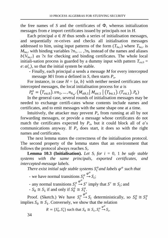
10 PROCESS ALGEBRAS FOR STUDYING SECURITY

34

the free names of S and the certificates of Φ, whereas initialization

messages from e import certificates issued by principals not in H.

Each principal a ∈ H thus sends a series of initialisation messages,

and sequentially re-ceives and checks all initialisation messages

addressed to him, using input patterns of the form (Tba,r) where Tba,r is

Mba,r with binding variables ?n1, ... ,?nk instead of the names and aliases

b{Vba,r} as ?x for checking and binding certificates. The whole local

initiali-sation process is guarded by a dummy input with pattern Tea,0 =

𝑒: 𝑎⟨_⟩, so that the initial system be stable.

- Finally, each principal a sends a message M for every intercepted

message M/i from a defined in S, then starts Pa.

For instance, in case H = {a, b} with neither nested certificates nor

intercepted messages, the local initialisation process for a is

𝑃𝑎𝑜 = (𝑇𝑒𝑎,0). 𝑣𝑛1, … , 𝑛𝑘𝑎 . (𝑀𝑎𝑏,1| 𝑀𝑎𝑒,1 | (𝑇𝑏𝑎,1). (𝑇𝑒𝑎,1). 𝑃𝑎)

In the general case, several rounds of initialisation messages may be

needed to exchange certifi-cates whose contents include names and

certificates, and to emit messages with the same shape one at a time.

Intuitively, the attacker may prevent Pa from running at all by not

forwarding messages, or provide a message whose certificates do not

match the certificates expected by Pa, but it could block all of a’s

communications anyway. If Pa does start, it does so with the right

names and certificates.

The next lemma states the correctness of the initialisation protocol.

The second property of the lemma states that an environment that

follows the protocol always reaches Si.

Lemma 10.3 (Initialisation). Let Si for i = 0, 1 be safe stable

systems with the same principals, exported certificates, and

intercepted-message labels.

There exist initial safe stable systems 𝑆𝑖𝑜and labels 𝜑𝑜 such that

- we have normal transitions 𝑆𝑖𝑜𝜑𝑜

→ 𝑆𝑖;

- any normal transitions 𝑆𝑖𝑜𝜑𝑜

→ 𝑆′ imply that 𝑆′ ≡ 𝑆𝑖; and

- 𝑆0 ≅ 𝑆1 if and only if 𝑆0𝑜 ≅ 𝑆1

𝑜.

Proof. (Sketch.) We have 𝑆𝑖𝑜𝜑𝑜

→ 𝑆𝑖 deterministically, so 𝑆0𝑜 ≅ 𝑆1

𝑜

implies 𝑆0 ≅ 𝑆1. Conversely, we show that the relation

𝑅 = {𝑆0′ , 𝑆1

′} such that 𝑆0 ≅ 𝑆1, 𝑆𝑖𝑜𝜑𝑜

→ 𝑆𝑖 ,

10 PROCESS ALGEBRAS FOR STUDYING SECURITY

35

and 𝜑 is a prwfix of a permutation of the lables of 𝜑𝑜} ∪≅

is a labelled bisimulation. (Intuitively, 𝜑 is the part of 𝜑𝑜 that has

already been enabled by the attacker.)

10.5 A Concrete Implementation

We are now ready to define the machines, relying on translations

from high-level terms and processes to keep track of their runtime state.

We systematically map high-level systems S to the machines, mapping

each principal a[Pa] of S to a PPT machine Ma that executes Pa. We

start by giving an outline of our implementation.

The implementation mechanisms are simple, but they need to be

carefully specified and com-posed. (As a non-trivial example, when a

machine outputs several messages, possibly to the same principals, we

must sort the messages after encryption so that their ordering on the

wire leaks no information on the computation that produced them.)

We use two concrete representations for terms: a wire format for

(signed, encrypted) mes-sages between principals, and an internal

representation for local terms. Various bitstrings rep-resent

constructors, principal identities, identifiers for names, and certificates.

Marshaling and unmarshaling functions convert between internal and

wire representations. When marshaling a locally restricted name

identifier ind for the first time, we draw a bitstring s of length ´

uniformly at random, associate it with ind, and use it to represent ind on

the wire. When unmarshaling a bitstring s into an identifier for a name,

if s is not associated with any local identifier, we create a new internal

identifier ind for the name, and also associate s with ind.

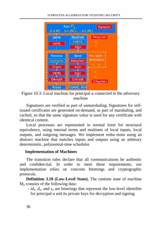
10 PROCESS ALGEBRAS FOR STUDYING SECURITY

36

Figure 10.3: Local machine for principal a connected to the adversary

machine

Signatures are verified as part of unmarshaling. Signatures for self-

issued certificates are generated on-demand, as part of marshaling, and

cached, so that the same signature value is used for any certificate with

identical content.

Local processes are represented in normal form for structural

equivalence, using internal terms and multisets of local inputs, local

outputs, and outgoing messages. We implement reduc-tions using an

abstract machine that matches inputs and outputs using an arbitrary

deterministic, polynomial-time scheduler.

Implementation of Machines

The transition rules declare that all communications be authentic

and confiden-tial. In order to meet these requirements, our

implementation relies on concrete bitstrings and cryptographic

protocols.

Definition 3.18 (Low-Level State). The runtime state of machine

Ma consists of the following data:

- ida, da, and sa are bitstrings that represent the low-level identifier

for principal a and its private keys for decryption and signing.

10 PROCESS ALGEBRAS FOR STUDYING SECURITY

37

- peers = {(idu, eu, vu) | u ∈ Prin} binds, for every principal, a low-level

identifier to public keys for encryption and signature verification.

- pa is a low-level representation of a local process running at a

(defined below).

- keycachea is a set of authentication keys for all received

messages. - signeda is a partial function from certificates issued by a to signature

values.

- namesa is a partial function from name identifiers to bitstrings.

The main machine components are depicted in Figure 10.3.

Before detailing the definitions of all the protocols presented if

Figure 10.3, we describe a complete run of the machine. Recall that Ma

is connected to the environment by two wires, ina and outa. The wire

format for messages is the concatenated bitstring idu_idv_msg where u

and v are the (apparent) sender and receivers and msg is some

encrypted, authenticated, marshaled message. When it receives such a

message (with idv = ida), Ma uses idu to dispatch msg to the receive

protocol (Definition 3.23) for remote principal u— there is an instance

of the receive protocol for each peer principal u. The protocol verifies

the freshness, integrity, and authenticity of the message, updates

keycachea, then returns a decrypted bitstring s. If a verification step

fails, the message is discarded.

At this stage, msg is a genuine message from u to a, but its content

is not necessarily well-formed. For instance u may have included a

certificate apparently issued by b but with an invalid signature. Content

validation occurs as s is unmarshaled (Definition 10.21) from its wire

format into some internal (trusted) representation parsea(s) of a high-

level term V. In particular, this trusted representation embeds a valid

signature for every certificate of V. After successful recep-tion and

unmarshaling, a representation m of the incoming message u:a⟨𝑉⟩ imay

react with an input within pa and trigger local computations. To this

end, a local interpreter (Definition 10.19) derived from the abstract

machine runs on pa | m. If the interpreter terminates, it yields a new

stable internal process p'a plus a set of outgoing messages X to be sent

to the network.

Each message a:ui⟨𝑉𝑖⟩ represented in X is then marshaled

(Definition 10.20) and passed to the instance of the send protocol

10 PROCESS ALGEBRAS FOR STUDYING SECURITY

38

(Definition 10.22) associated with the intended recipient ui. The

resulting bitstrings, all in wire format, of the form ida_idui_msgi, are

eventually sorted (by receiving principal, then encrypted value msgi)—

to ensure that their ordering leaks no informa-tion on their payload or

their internal production process—and written on outa. A final done

bitstring is issued and the machine terminates. (Hence, for instance, if p

does not react with m, the machine simply writes done on outa and

terminates.)

Next, we describe in turn each of the components of the local

machine.

Low-level Processes Reductions

The internal representation of terms uses the same grammar as in

the high-level language except for atomic subterms: principals u are

boxed, fixed-sized bitstrings prin(idu) (lprin); free names are boxed,

bitstrings name(ind) where ind is an internal identifier for names; and

certificate labels are linear-sized bitstrings s such that either s is a valid

signature for the certificate or s = 0 and the certificate is self-issued.

Bound variables and names may still occur in terms under input guards.

Definition 10.19 (Internal Reductions). The local reduction

algorithm refines the abstract machine as follows:

- it represents the multisets X, M, and G using internal terms;

- it uses a deterministic, polynomial-time, complete scheduler;

- instead of lifting new name restriction vn.Q, it generates a new

identifier ind (possibly incrementing an internal counter) and

substitutes name(ind) for all bound instances of the n in Q.

Marshaling and Unmarshaling Protocols

These algorithms are responsible for processing messages that are

about to be sent to (that were received from) the network. The

marshaling process transforms each internal term into a bit-string to be

sent over the network, and the unmarshal algorithm attempts to

transform a bitstring received from the network to a (trusted) internal

term; it may instead return an error if the mes-sage is not well-formed,

or if the signature of an included certificate cannot be verified. In any

of these cases the entire message is discarded.

10 PROCESS ALGEBRAS FOR STUDYING SECURITY

39

We use a fixed, injective function from all constructors plus name

and prin to bitstrings of a given fixed size; we still write f, name, prin

for the corresponding bitstrings. We write s_s' for the bitstring obtained

by concatenating s and s'.

Definition 10.20 (Marshaling). Let Σ = (G, S, V) be a signature

scheme. The function ⟦•⟧ maps principal’s internal representations of

closed terms to bitstrings, as follows:

⟦𝑛𝑎𝑚𝑒 (𝑖𝑛𝑑)⟧ = 𝑛𝑎𝑚𝑒_𝑛𝑎𝑚𝑒𝑠(𝑖𝑛𝑑) 𝑎𝑑𝑑𝑖𝑛𝑔 𝑛𝑎𝑚𝑒𝑠(𝑖𝑛𝑑) = 𝑠 ← {0,1}η when undefined

⟦𝑝𝑟𝑖𝑛(𝑠)⟧ = 𝑝𝑟𝑖𝑛_𝑠 ⟦𝑓(𝑣1, … , 𝑣𝑛)⟧ = 𝑓_⟦𝑣1⟧_ ..._ ⟦𝑣𝑛⟧ when f ∉ {name, prin, cert}

⟦𝑣1{𝑣2}𝑠⟧ = 𝑐𝑒𝑟𝑡_⟦𝑣1⟧_⟦𝑣2⟧_ s when 𝑠 ≠ 0

⟦𝑣1{𝑣2}0⟧ = 𝑐𝑒𝑟𝑡_⟦𝑣1⟧_⟦𝑣2⟧_ signed (𝑣1{𝑣2}0) when

𝑣1 = 𝑝𝑟𝑖𝑛(𝑖𝑑𝑏), 𝑏 ∈ 𝐻

adding signed (𝑣1{𝑣2}0) = 𝑆(𝑠𝑏 , ⟦𝑣2⟧𝑏) when undefined.

We denote by ⟦•⟧𝑎 the marshaling procedure for machine Ma that

uses only uses tables namesa and signeda, that is, names = namesa and

signed = signeda.

We prove as an invariant that for all certificates of the form v1{v2}0

in pa, v1 = prin(ida), hence ⟦•⟧𝑎 is defined for all internal

representations of terms of Ma.

We assume that after marshalling, and before sending, all our

messages are padded to a fixed length that is given by the polynomial

ms(η), a parameter of the implementation. We could have assumed that

this was not the case and if so, we needed to consider this difference of

length in our high-level semantics. We could have done it using sorts

and sizes for input and output messages.

Definition 10.21 (Unmarshaling). Let Σ = (G, S, V) be a signature

scheme. The partial function parse(•) maps bitstrings to internal

representations of closed terms, as follows, and fails in all other cases.

parse(name_s) = name(ind) when, there is ind:names(ind) = s

otherwise if |s| = η then

ind = |dom(names)| + 1 and

add names(ind) = s

parse(prin_s) = prin(s) when |s| = 𝑙𝑝𝑟𝑖𝑛 and (s, 𝑒𝑠, 𝑣𝑠) ∈ peers

parse(F_𝑠1_... 𝑠𝑛) = 𝑓(𝑣1, … , 𝑣𝑛) when f ∉ {name, prin, cert}

10 PROCESS ALGEBRAS FOR STUDYING SECURITY

40

has arity n parse(𝑠𝑖) = 𝑣𝑖 for 𝑖 = 1. . 𝑛 parse(cert_𝑠1_𝑠2_𝑠3) = 𝑣1{𝑣2}𝑠 when, for some (𝑖𝑑𝑢, 𝑒𝑢, 𝑢𝑢) ∈

peers, parse(𝑠1) = prin(𝑖𝑑𝑢)= 𝑣1, parse(𝑠2)= 𝑣2 V(𝑢𝑢, 𝑠2, 𝑠3) = 1 s = if signed(𝑣1{𝑣2}0) = 𝑠3 then else 𝑠3 We denote by parsea(•) the unmarshaling procedure for machine Ma

that uses only uses tables namesa and signeda, that is, names = namesa

and signed = signeda.

Unmarshaling includes signature verification for any received

certificate, and is otherwise standard; it is specified here as a partial

function from strings to internal representations, and can easily be

implemented as a parser. Our treatment of self-issued certificates with

label 0 reflects our choice of internal representations: 0 stands for the

(unique) signature generated by the local machine for this certificate

content, the first time this certificate is marshaled. (In addition, the

adversary may be able to derive a variant of this certificate with a

different signature, unmarshaled with a non-zero label; such certificates

are then treated using the default case for marshaling.)

Although we give a concrete definition of ⟦•⟧, parse(•), and

message formats, our results only depend on their generic properties.

We only require that, for a given local machine, every string be

unmarshaled to at most one internal term, whose marshaling yields

back the original string, that is, parsea

denotes the internal representation of a for V . We define

formally in Definition 10.25.) For simplicity, we have that the length of

the string be a function of the structure of the internal term and of the

security parameter.

Sending and Receiving Protocols

Two important pieces of our systems are the sendb and receiveb

protocols. There are one pair of these for each other principal. The send

protocol defined below, ensures that, as abstracted in the high-level

semantics, all communications are opaque for the adversary using

10 PROCESS ALGEBRAS FOR STUDYING SECURITY

41

public-key encryption, and that the communication is authentic, using

authentication and signature schemes. This protocol takes a bitstring s

(containing a marshaled message from a to u), protects it, and returns it

in wire format. Conversely, the receiving protocol takes a message in

wire format presumably from u, verifies it, and returns its payload. We

also request robustness against replay attacks; after decryption, we

reject any message whose authentication key is already recorded.

These protocols are intended as a simple example; other choices are

possible. We may for instance consider long term shared keys between

principals, in order to reduce the overhead of public-key cryptography.

If we decide to do so, we should introduce a nonce in the message that

is encrypted in Step 3.

Definition 10.22 (Sending to u). Let П = (K, E, D), ∑ = (G, S, V),

and ∆ = (𝐺∆, A, C) be respectively an encryption, signature, and

authentication schemes. Given a bitstring s, the sendu protocol

- generates a fresh authentication key k ← 𝐺∆(1η);

- computes 𝑚 = 𝑠_𝑖𝑑𝑎_𝑘_𝑆(𝑠𝑎, 𝑘𝑖𝑑𝑢)_𝐴(𝑘, 𝑠);

- computes msg = E(eu, m); and

- retur ida _idu _msg.

Definition 10.23 (Receiving from u). Let П = (K, E, D), ∑ = (G,

S, V), and ∆ = (𝐺∆, A, C) be respectively an encryption, signature, and

authentication schemes. Given a bitstring idu ida msg, the receiveu

protocol

- computes s_ idu _k _ssig _sauth = D(da, msg);

- checks that there is an entry (idu, eu, vu) ∈ peers with V(vu,

k_ida, ssig) = 1;

- checks that C(k, s, sauth ) = 1;

- checks that k is not in keycache, and adds it to keycache;

- returns s.

The entire message is discarded if any step of the protocol fails.

Mapping High-Level Systems to Low-Level Machines

In order to systematically relate the runtime state of low-level

machines to the abstract state of high-level systems, we define an

associated shadow state. This structure provides a consistent

interpretation of terms across machines. In combination, a system and

its shadow state deter-mine their implementation, obtained as a

10 PROCESS ALGEBRAS FOR STUDYING SECURITY

42

compositional translation of terms, local processes, and configurations.

(This state is shadow as it need not be maintained at runtime in the low-

level implementation; it is used solely as an abstraction to reason about

the correctness of our imple-mentations.) We further partition this state

into public parts, intended to be part of the attacker’s knowledge, and

private parts.

Definition 10.24 (Shadow State). Let S = Φ 𝑣�̃�. 𝐶 be a system

such that the configuration 𝐶 = П𝑎∈𝐻𝑎[𝑃𝑎]| П𝑖∈𝐼 𝑀/𝑖 is in normal

form. A shadow state for S, written D, consists of the following data

structure:

- prin ∈ Prin → ({0,1}η)5 is a function from u ∈ Prin to bitstrings

idu, eu, vu, du, su such that u → idu is injective, and for every u

∈ H, we have (eu, du) ←K(1η), and (vu, su) ← G(1η).

- The bitstrings idu , eu , vu are public for all u ∈ Prin; du and su

are public if u ∈ Prinn\H.

- name ∈ Name → {0,1}η is a partial injective function defined at

least on every name that occurs free in S, and names that occur in

Φ, D.certval or D.wire.

- The bitstring name(m) is public for every name m ∉ �̃�.

- ni is a family of partial injective functions ni a : Name → {0,1}η

for each a ∈ H, defined at least for all names of Pa that are not

locally-restricted.

- certval is a partial function from certificates 𝑢{𝑉}𝑙 to s ∈ {0,1}η

defined at least on the certificates of Φ, D.wire, and all

certificates of 𝑃𝑎 of the form 𝑎{𝑉}𝑙 with 𝑙 ≠ 0 or 𝑢{𝑉}𝑙 with

𝑢 ≠ 𝑎. It is also defined for all the certificates in V such that

𝑢{𝑉}𝑙 is defined in certval, certval satisfies the following

property: if certval (𝑢{𝑉}𝑙) = s, then

- The bitstrings s and del are public.

- - wire is a partial function from indices i to (M, k, s, del) defined at

least on I, where 𝑀 = 𝑎: 𝑏⟨𝑉⟩ with a, b ∈ H, and del = 0 if i ∈ I

and del = 1 otherwise. The bitstrings s and k are the output and

the authentication key produced by 𝑠𝑒𝑛𝑑𝑏 on input .

10 PROCESS ALGEBRAS FOR STUDYING SECURITY

43

- keycache is a function from 𝑎 ∈ 𝐻 to sets of bitstrings such that,

if exists an i with wire(i) = (M, k, _, 1) with M to a, then k ∈

keycache(a).

- 𝑚𝑠𝐷(η) is a polynomial that sets the padding-size of the

implementations of S.

Intuitively, wire records all messages sent between honest

principals; keycache(a) records the authentication keys of all messages

received by a so far; it contains at least the keys of mes-sages in wire

that were already received by a. When D is clear from the context, we

write prin(a) instead of D.prin(a), and similarly for the other

components of D. We denote by public(D) the binary representation of

the public parts of D. When we are not interested in the specific bit-

strings, we call it shape of D.

Definition 10.25 (Concrete Terms and Processes). A shadow

state D and a set of principals

X ⊆ Prin, define a partial map from high-level terms V to internal

terms as follows:

𝑛𝐷,𝑋 = {𝑓𝑔𝑏

We extend this map to translate local processes to low-level

processes, as follows: high-level terms within local processes are

translated as above, except for variables and locally-restricted names

(left unchanged); high-level patterns are translated by applying the

translation to all high-level terms in the pattern and leaving the rest

unchanged; local processes P are translated to internal processes PD,X

by translating their high-level terms to internal terms.

As a corollary, we have that if D is a shadow state for S, and a ∈

Prin then • D,a is defined for every subterm and subprocess of S and D (•

10 PROCESS ALGEBRAS FOR STUDYING SECURITY

44

D,a denotes • D, fag

). We often write V instead of V D,a

when D and a are

clear from the context. Our intent is that, with overwhelming

probability, we have V = V' iff V

D,a = V

' D,a whenever D defines these

representations.

We would like to point out that the previous definition is well-

formed. One should first notice that we do not translate high-level

terms (hence, high-level certificates) with variables and locally-

restricted names. Hence, when applying 𝑢{𝑉}𝑙𝐷,𝑎

, we can be sure that

the certificate was previously generated and hence defined in D:certval.

Definition 10.26(System Implentations). Let S be a system with

shadow state D. The implementation of S and D is the collection of

machines M(S,D) = (𝑀𝑎(𝑆, 𝐷))𝑎∈𝐻 where each machine 𝑀𝑎(𝑆, 𝐷) has

the following state:

- ida , da , sa , peersa are read from D:prin;

- pa = Pa D,a

;

- keycachea = keycache(a);

- signeda( a{V }0D,a

) = certval(a{V}0) when defined;

- namesa(nia(n)) = name(n) when defined,

and uses ⟦•⟧𝑎 and parsea(•) as the marshaling and unmarshaling

algorithms, and msD(•) as the padding size.

10.11 Main Results

In this section we present the main results of this Chapter.

Throughout this section we assume that the encryption scheme П = (K,

E, D) is CCA-2 secure, and the signature scheme Σ = (G, S, V) and

authentication scheme ∆ = (𝐺∆, A, C) are CMA-secure.

Our main theorems are stated in terms of arbitrary systems S. As it

is convenient to have a for-mulation of these theorems in terms of

arbitrary systems, one should not forget that an arbitrary system S is

obtained starting from an initial system So that has no shared names or

certificates and no intercepted messages so, whenever we refer to a

system S, we are in fact referring to its initial state So plus its

initialisation procedure. The same happens with the implementations

and for that we introduce the notion of valid shadow. Intuitively, a

shadow D is a valid shadow for S, if there is an interactive run

(Definition 3.1) that starts with M(So, D

o) and leads the machine to state

M(S; D), where D± is the shadow obtained from D by erasing

10 PROCESS ALGEBRAS FOR STUDYING SECURITY

45

everything except D:prin. Do is called an initial shadow for S. We

denote by Ao[M(So, D

o)] → sr(M(S, D)) such run, where sr is the

bitstring returned by Ao at the end of the run.

Accordingly, we define a low level run starting from S with (valid)

shadow D against A, written A[M(S, D)] → sr(M), as (Ao ; A)[M(So,

Do)] → sr(M) where (Ao; A) represents an adversary that first runs Ao

and then runs A. Definition 10.27 (Valid Shadow). Let S be a safe system with

shadow D. We say that D is a valid shadow for S if there exist an initial

safe system So with initial shadow D

±, normal transitions S

o 𝜑𝑜

→ S, and a

PPT algorithm A± such that Ao[M(So, D

o)] →public(D)(M(S, D)), and

msD(η) ≥ 𝑚𝑎𝑥⌈𝑀⌉≤𝑐⌈⟦𝑀

𝐷⟧⌉ where c is the constant given by the safety

condition and ⟦𝑀𝐷⟧ is the result of marshaling the low-level

representations of M.

We say that D is a valid shadow for two safe systems S1 ≅ S2, if

the same Ao initialises both M(S1, D) and M(S2, D), and msD(η) ≥

𝑚𝑎𝑥⌈𝑀⌉{𝑐1,𝑐2}⌈⟦𝑀𝐷⟧⌉, where c1 and c2 are the constants given by the

safety condition of S1 and S2 respectively.

Our first theorem expresses the completeness of our high-level

transitions: every low-level attack can be described in terms of high-

level transitions. More precisely, the probability that an interaction with

a PPT adversary yields a machine state unexplained by any high-level

transitions is negligible.

Theorem 10.4 (Completeness for Reachable States). Let S be a

safe stable system, D a valid

shadow for S, and A a PPT algorithm.

The probability that A[M(S, D)] completes and leaves the

system in state M' with M

' ≠

M(S', D' ) for any normal transitions S 𝜑→ S' with valid shadow D

is negligible.

Proof Sketch. We just sketch the proof and refer the reader to

Appendix C for the full construc-tions and proofs of the associated

lemmas. The proof is done by tracing the cases when the behaviour of

machine M(S, D) is not in accordance with the high-level semantics and

check-ing that the probability of occurrence of such cases is negligible.

A more detailed sketch is the following:

10 PROCESS ALGEBRAS FOR STUDYING SECURITY

46

- We start by defining variants of M(S, D) called the defensive

variants M̅ (S, D) (Defini-tion C.1). These machines behave like

M(S, D) but include an extra wire where a failure signal is sent

whenever the low-level interaction is not in accordance with the

high-level se-mantics. The reader should be aware that these

machines are just used as a proof technique, hence there is no

need to implement it. All our results are stated in terms of M(S,

D).

- The second step is to create a machine �̅�0̃(S, D) that behaves like

M(S, D) but has a com-mon state for all machines Ma(S, D)

(Definition C.5). This is the same as having one single machine

that includes all the Ma(S, D) machines, for all a ∈ H. We show

that M(S, D) is equivalent to �̅�0̃ (S; D).

- The third step is to define �̅� (S, D). This is the extreme version

of �̅��̃� (S, D) where all the encrypted messages are 0’s and no

signing is ever performed.

Then we have two different arguments. The first is the partial

completeness of �̅� (S, D), �̅� (S, D), and the failure of �̅�(S, D).

- We show that all runs of �̅�(S, D) and �̅�(S, D), where the failure

signal is not sent are in confor mance with the high-level

semantics (Lemma C.6 and Lemma C.7).

- We show that the probability that the failure signal is issued by

N(S; D) machine is negligible by reducing it to the security of the

encryption, authentication and signing schemes (Lemma C.8).

The second argument is that �̅�(S, D) is indistinguishable from �̅�(S,

D), hence the failure of the former implies the failure of the latter,

which only happens with negligible probability. This is done as

follows:

- �̅��̃�(𝑆, 𝐷) machines are parameterised by �̃� = (𝑛𝑎)𝑎∈𝐻. This

parameter defines how many messages to each honest principal

will be “fake” (a fake message is one where we encrypt 0’s

instead of the real bitstring). Whenever na is reached, it starts

behaving like �̅�a(S, D). For the fake messages we keep an

internal table that associates the fake bitstring to the real message

so that we can proceed with the correct value when the fake

message is provided back to the machine. With a standard

10 PROCESS ALGEBRAS FOR STUDYING SECURITY

47

cryptographic argument we show that distinguishing �̅��̃�(S, D)

from �̅��̃�+1 (S, D), where �̃� + 1 has all the components equal to �̃�

except for na that we replace by na + 1 for some principal a

(Lemma C.12).

- We show via a cryptographic argument that for all PPT

adversaries, �̅�(S, D) is indistin-guishable from �̅�(S, D) (Lemma

C.13, C.14, and C.15).

This concludes our proof.

Finally, main result states the soundness of equivalence: to show that

the machines that implement two stable systems are indistinguishable,

it suffices to show that they are safe and bisimilar. We just need an

extra condition that the padding size is the same in both cases.

Theorem 10.5 (Soundness for Equivalences). Let S1 and S2 be

safe stable systems, D a valid shadow for both S1 and S2.

If S1 ≅ S2, then M(S1, D) ≈ M(S2, D).

Proof Sketch. For this theorem we also refer the reader to Appendix

C for the full proofs of the associated lemmas. The proof is done

reusing some of the previous lemmas, in particular Lemma C.15 and

with the special Lemmas C.16 and C.17. This lemmas state that for

equivalent systems S1 and S2 the probabilities of failure of �̅�(S1, D) and

�̅�(S2, D) are the same up to negligible probability.

Advancement questions

1. Why does the algebras are widely used in the study of security

of concurrent systems?

2. On what stages we are able to define the high-level semantics?

3. What the CFGBLOCK and CFGFWD rules do?

4. What is the scheduler algorithm?

5. What have we do if we quantify over all local processes?

6. What protocol was used as benchmark to verivy the presented

framework?

7. Name the roles of the electronic protocol.

8. What the representations for terms do we use?

10 PROCESS ALGEBRAS FOR STUDYING SECURITY

48

9. Does the internal representation of terms uses the same

grammar as in the high-level language except for atomic

subterms?

10. What pieces of the system sendb and receiveb protocols are

used?

REFERENCES

[1] Pedro Miguel dos Santos Alves Madeira Adão Formal

Methods for the Analysis of Security Protocols / Pedro Miguel dos

Santos Alves Madeira Adão // PhD diss., INSTITUTO SUPERIOR

TĖCNICO. – 2006.

[2] Milner R. Communication and Concurrency / R. Milner. -

Prentice Hall, 1989. – 256p.

[3] Lowe G. An attack on the needham-schroeder public-key

authentication protocol.Information / G. Lowe. // Processing Letters. -

1995. -Vol56(3). -p131–133.

[4] Lowe G. Breaking and fixing the Needham-Shroeder public-

key protocol using FDR. In Tiziana Margaria and Bernhard Steffen,

editors, Proceedings of the 2nd International Workshop on Tools and

Algorithms for the Construction and Analysis of Systems (TACAS),

volume 1055 of Lecture Notes in Computer Science / G. Lowe. //

Springer-Verlag. -1996. -p147–166.

[5] Abadi M. A calculus for cryptographic protocols: The Spi

Calculus. Information and Computation / M.Abadi, A.D. Gordon // Full

version available as SRC Research Report 149, January 1998. –January

1999, -Vol148(1). -p1–70.

[6] Milner R. Communicating and Mobile Systems : The pi-

Calculus. / R.Milner. - Cambridge University Press, June 1999, -31p.

[7] Abadi M. Mobile values, new names, and secure

communication / M.Abadi, Cédric Fournet // In 28th ACM Symposium

on Principles of Programming Languages (POPL). -2001. -p104–115.

[8] Mart´ ın Abadi. Secure implementation of channel

abstractions / Mart´ ın Abadi, Cédric Fournet, Georges Gonthier //

Information and Computation. -2002. -Vol174(1). -p37–83.

10 PROCESS ALGEBRAS FOR STUDYING SECURITY

49

[9] Blanchet B. Automated verification of selected equivalences

for security protocols / B. Blanchet, M. Abadi, C. Fournet // In

Proceedings of the 20th IEEE Symposium on Logic in Computer

Science (LICS). – 2005. – p. 331–340.

[10] Rackoff C. and Simon D.R. Non-interactive zero-knowledge

proof of knowledge and chosen ciphertext attack / C. Rackoff, D.R.

Simon // In Feigenbaum. – 1991. – p. 433–444.

[11] Goldwasser S. A digital signature scheme secure against

adaptive chosen-message attacks / S. Goldwasser, S. Micali, and R.L.

Rivest // SIAM Journal on Computing. -1988. -Vol17(2). -p281–308.

[12] Goldwasser S. Probabilistic encryption / S. Goldwasser and S.

Micali // Journal of Computer and Systems Sciences. - 1984. -Vol28(2).

– p. 270–299.

[13] Martin Abadi Authentication primitives and their compilation

/ Martin Abadi, Cédric Fournet, and Georges Gonthier // In Proceedings

of the 27th ACM Symposium on Principles of Programming Languages

(POPL 2000). -2000. -p302–315. ACM.

[14] Backes M. A cryptographically sound Dolev-Yao style

security proof of an electronic payment system / M. Backes and M.

Dürmuth // In CSFW05 [CSF05] –p. 78–93.

[15] Bellare M. iKP — a family of secure electronic payment

protocols / M. Bellare, J. Garay, R. Hauser, A. Herzberg abd H.

Krawczyk, M. Steiner, G. Tsudik, and M. Waidner // In Proceedings of

the 1st USENIX Workshop on Electronic Commerce. - 1995.

[16] Bellarer M.. Design, implementation, and deployment of the

ikp secure electronic payment system / M. Bellare, J. Garay, R. Hauser,

A. Herzberg abd H. Krawczyk, M. Steiner, G. Tsudik, E. Van

Herreveghen, and M. Waidner // IEEE Journal on Selected Areas in

Communications. -2000. Vol18(4). –p. 611–627.

[17] Backes M. A composable cryptographic library with nested

operations. In S. Jajodia, V. Atluri, and T. Jaeger, editors / M. Backes,

B. Pfitzmann, and M. Waidner // Proceedings of the 10th ACM

Conference on Computer and Communications Security (CCS). -2003.

–Vol15. –p. 220–230.

[18] Lincoln P. A probabilistic polynomial-time framework for

protocol analysis. In M. Reiter, editor / P. Lincoln, J. C. Mitchell, M.

10 PROCESS ALGEBRAS FOR STUDYING SECURITY

50

Mitchell, and A. Scedrov // Proceedings of the 5th ACM Conference on

Computer and Communications Security (CCS). -1998. –p. 112–121.

[19] Martin Abadir. Authentication primitives and their

compilation / Martin Abadi, Cédric Fournet, and Georges Gonthier // In

Proceedings of the 27th ACM Symposium on Principles of

Programming Languages (POPL 2000). -2000. – p. 302–315.

11 A PROCESS ALGEBRA FOR REASONING ABOUT QUANTUM SECURITY

51

CHAPTER 11. A PROCESS ALGEBRA FOR REASONING

ABOUT QUANTUM SECURITY

Content of the chapter 11

CHAPTER 11. A Process Algebra for Reasoning About Quantum

Security ................................... Ошибка! Закладка не определена.

Introduction ............................ Ошибка! Закладка не определена.

11.1 Process Algebra .............. Ошибка! Закладка не определена.

11.2 Quantum polynomial machinesОшибка! Закладка не определена.

11.3 Process algebra ............... Ошибка! Закладка не определена.

11.4 Semantics ........................ Ошибка! Закладка не определена.

11.4 Observations and observational equivalenceОшибка! Закладка не определена.

11.6 Emulation and Composition TheoremОшибка! Закладка не определена.

11.7 Quantum Zero-Knowledge ProofsОшибка! Закладка не определена.

11 A PROCESS ALGEBRA FOR REASONING ABOUT QUANTUM SECURITY

52

Introduction

Security protocols are, in general, composed by several agents

running in parallel, where each agent computes information (bounded

by polynomial-time on the security parameter) and exchange it with

other agents. In the context of quantum processes, the computation is

bounded by quantum polynomial-time and the information exchanged

is supported by qubits. In this Chapter, the problem of defining

quantum security properties is addressed using a quantum polynomial-

time process algebra. This approach is highly inspired in [1, 2, 3 ].

The process algebra is introduced together with the logarithmic cost

random access machine. Both the syntax and the semantics of the

process algebra are clearly established, and the section is concluded by

presenting the notion of observational equivalence. Sections are

devoted to emulation and its composition theorem, and quantum zero-

knowledge is defined using process emulation.

11.1 Process Algebra

In the context of security protocols it is common to consider a

security parameter . In the case of quantum protocols we will

also consider such parameter in order to bound the quantum complexity

of the principals and adversaries. From now on, the symbol is

reserved to designate such security parameter. The role of this

parameter is twofold: it bounds to a polynomial on the number of

qubits that can be sent through channels, and it bounds all the

computation to quantum polynomial time (on ). We now detail these

aspects culminating with the presentation of the process algebra

language.

11.2 Quantum polynomial machines

The computational model we adopted to define quantum

polynomial machine is based on the logarithmic cost random access

machine [4] and it is quite similar to the quantum random access

machine in [5]. We consider a hybrid model using both classic and

quantum memory.

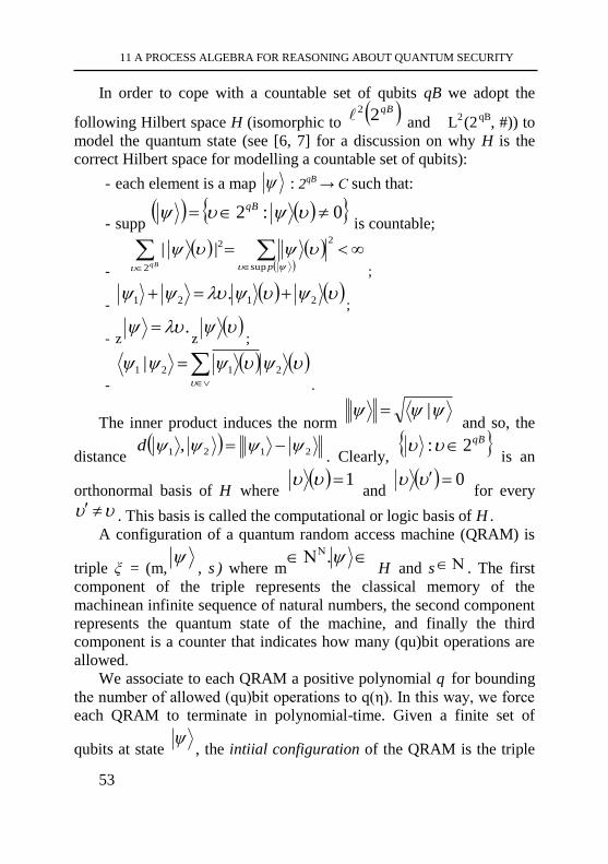
11 A PROCESS ALGEBRA FOR REASONING ABOUT QUANTUM SECURITY

53

In order to cope with a countable set of qubits qB we adopt the

following Hilbert space H (isomorphic to qB22 and L2(2

qB, #)) to

model the quantum state (see [6, 7] for a discussion on why H is the

correct Hilbert space for modelling a countable set of qubits):

- each element is a map : 2qB → C such that:

- supp 0:2 qB

is countable;

-

qB p2 sup

22||

;

- 2121 .

;

- z. z

;

-

2121 |

.

The inner product induces the norm |

and so, the

distance 2121 , d

. Clearly, qB2:

is an

orthonormal basis of H where 1

and 0

for every

. This basis is called the computational or logic basis of H . A configuration of a quantum random access machine (QRAM) is

triple ξ = (m,

, s ) where m .

H and s . The first

component of the triple represents the classical memory of the

machinean infinite sequence of natural numbers, the second component

represents the quantum state of the machine, and finally the third

component is a counter that indicates how many (qu)bit operations are

allowed.

We associate to each QRAM a positive polynomial q for bounding

the number of allowed (qu)bit operations to q(η). In this way, we force

each QRAM to terminate in polynomial-time. Given a finite set of

qubits at state

, the intiial configuration of the QRAM is the triple

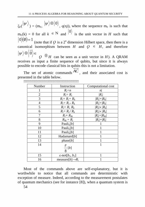
11 A PROCESS ALGEBRA FOR REASONING ABOUT QUANTUM SECURITY

54

ξ0(

) = (m0 , 0

, q(η)), where the sequence m0 is such that

m0(k) = 0 for all k and 0

is the unit vector in H such that

100 (note that if Ϙ is a 2

n dimension Hilbert space, then there is a

canonical isomorphism between H and Ϙ H , and therefore

0 Ϙ H can be seen as a unit vector in H ). A QRAM

receives as input a finite sequence of qubits, but since it is always

possible to encode classical bits in qubits this is not a limitation.

The set of atomic commands CA~~

, and their associated cost is

presented in the table below. !!!!!!!!!!!!!!!!!!!!!!!!!!!!!!!!!!!!!!!!!!!!!!!!

Number Instruction Computational cost

1 Ri=n n|

2 Ri= Rj |Rj|

3 Ri= Rj+ Rk |Rj|+|Rk|

4 Ri= Rj ˗ Rk |Rj|+|Rk|

5 Ri= Rj Rk |Rj| |Rk|

6 Ri= Rj / Rk |Rj| |Rk|

7 Ri= RRj |Rj|+|RRj|

8 RRj = Rj |Rj|+|Rj|

9 Paulix[b] 1

10 Pauliy[b] 1

11 Pauliz[b] 1

12 Hadamard[b] 1

13 phase[b] 1

14

8

[b]

1

15 c˗not[b1, b2] 1

16 measure[b]→Ri 1

Most of the commands above are self-explanatory, but it is

worthwhile to notice that all commands are deterministic with

exception of measure. Indeed, according to the measurement postulates

of quantum mechanics (see for instance [8]), when a quantum system is

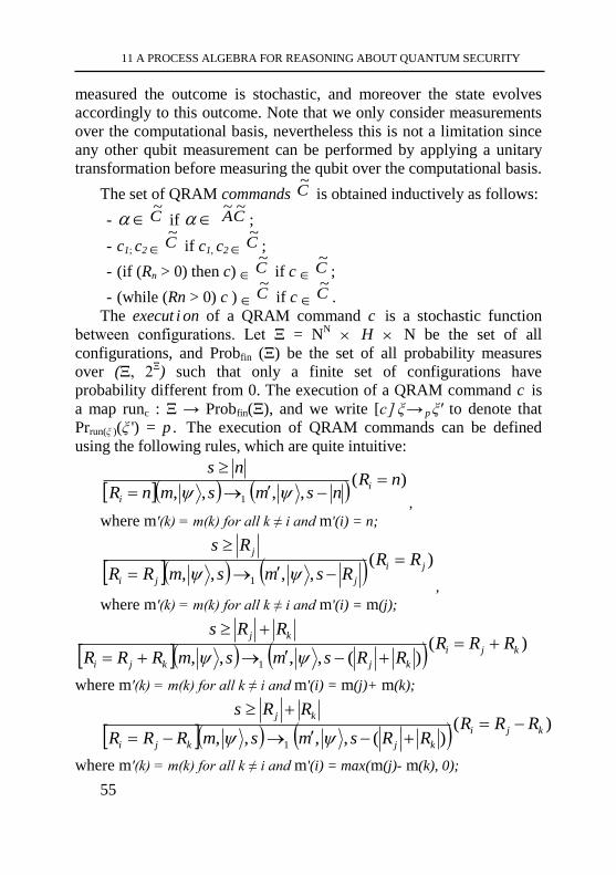
11 A PROCESS ALGEBRA FOR REASONING ABOUT QUANTUM SECURITY

55

measured the outcome is stochastic, and moreover the state evolves

accordingly to this outcome. Note that we only consider measurements

over the computational basis, nevertheless this is not a limitation since

any other qubit measurement can be performed by applying a unitary

transformation before measuring the qubit over the computational basis.

The set of QRAM commands C~

is obtained inductively as follows:

- C~

if CA~~

;

- c1; c2 C~

if c1, c2 C~

;

- (if (Rn > 0) then c) C~

if c C~

;

- (while (Rn > 0) c ) C~

if c C~

.

The execut i on of a QRAM command c is a stochastic function

between configurations. Let Ξ = NN H N be the set of all

configurations, and Probfin (Ξ) be the set of all probability measures

over (Ξ, 2Ξ) such that only a finite set of configurations have

probability different from 0. The execution of a QRAM command c is

a map runc : Ξ → Probfin(Ξ), and we write [c] ξ→ p ξ' to denote that

Prrun(ξ )(ξ ') = p . The execution of QRAM commands can be defined

using the following rules, which are quite intuitive:

)(

,,,, 1

nRnsmsmnR

nsi

i

,

where m'(k) = m(k) for all k ≠ i and m'(i) = n;

)(

,,,, 1

ji

jji

jRR

RsmsmRR

Rs

,

where m'(k) = m(k) for all k ≠ i and m'(i) = m(j);

)(

)(,,,, 1

kji

kjkji

kjRRR

RRsmsmRRR

RRs

where m'(k) = m(k) for all k ≠ i and m'(i) = m(j)+ m(k);

)(

)(,,,, 1

kji

kjkji

kjRRR

RRsmsmRRR

RRs

where m'(k) = m(k) for all k ≠ i and m'(i) = max(m(j)- m(k), 0);

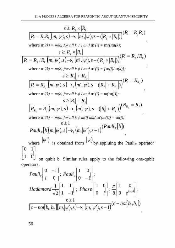
11 A PROCESS ALGEBRA FOR REASONING ABOUT QUANTUM SECURITY

56

)(

)(,,,, 1

kji

kjkji

kjRRR

RRsmsmRRR

RRs

,

where m'(k) = m(k) for all k ≠ i and m'(i) = m(j)m(k);

)(

)(,,,, 1

kji

kjkji

kjRRR

RRsmsmRRR

RRs

,

where m'(k) = m(k) for all k ≠ i and m'(i) = [m(j)/m(k)];

)(

)(,,,, 1

j

jj

j

Ri

RjRi

Rj

RRRRsmsmRR

RRs

,

where m'(k) = m(k) for all k ≠ i and m'(i) = m(m(j));

)(

)(,,,, 1

jR

jijR

jiRR

RRsmsmRR

RRs

j

j

,

where m'(k) = m(k) for all k ≠ m(i) and m'(m(i)) = m(j);

)(

1,,,,

1

1

bPaulismsmbPauli

sX

X

,

where

is obtained from

by appluing the PauliX operator

01

10

on qubit b. Similar rules apply to the following one-qubit

operators:

0

0

i

iPauliY ;

10

01ZPauli ;

11

11

2

1Hadamard ;

iPhase

0

01;

40

01

8

ie

;

),(

1,,,,,

121

121

bbnotcsmsmbbnotc

s

,

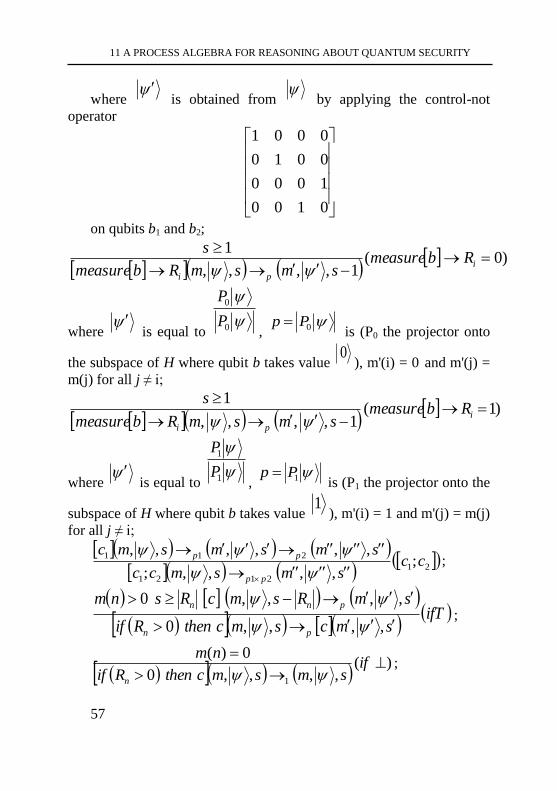
11 A PROCESS ALGEBRA FOR REASONING ABOUT QUANTUM SECURITY

57

where

is obtained from

by applying the control-not

operator

0100

1000

0010

0001

on qubits b1 and b2;

)0(

1,,,,

1

i

pi

RbmeasuresmsmRbmeasure

s

where

is equal to

0

0

P

P

, 0Pp

is (P0 the projector onto

the subspace of H where qubit b takes value 0

), m'(i) = 0 and m'(j) =

m(j) for all j ≠ i;

)1(

1,,,,

1

i

pi

RbmeasuresmsmRbmeasure

s

where

is equal to

1

1

P

P

, 1Pp

is (P1 the projector onto the

subspace of H where qubit b takes value 1

), m'(i) = 1 and m'(j) = m(j)

for all j ≠ i;

21

2121

211;

,,,,;

,,,,,,cc

smsmcc

smsmsmc

pp

pp

;

ifTsmcsmcthenRif

smRsmcRsnm

pn

pnn

,,,,0

,,,,0

;

)(

,,,,0

0)(

1

if

smsmcthenRif

nm

n ;

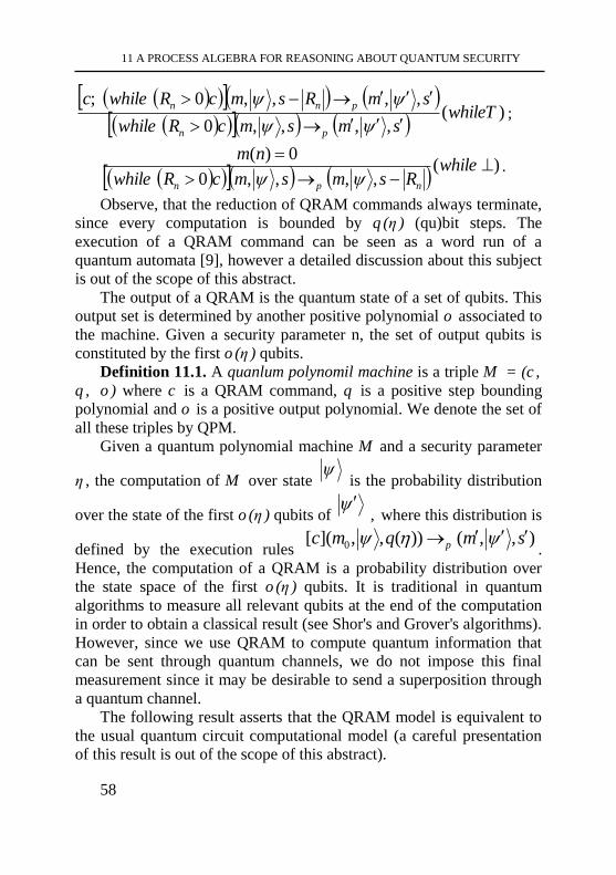
11 A PROCESS ALGEBRA FOR REASONING ABOUT QUANTUM SECURITY

58

)(,,,,0

,,,,0;whileT

smsmcRhilew

smRsmcRhilewc

pn

pnn

;

)(

,,,,0

0)(

while

RsmsmcRhilew

nm

npn .

Observe, that the reduction of QRAM commands always terminate,

since every computation is bounded by q (η ) (qu)bit steps. The

execution of a QRAM command can be seen as a word run of a

quantum automata [9], however a detailed discussion about this subject

is out of the scope of this abstract.

The output of a QRAM is the quantum state of a set of qubits. This

output set is determined by another positive polynomial o associated to

the machine. Given a security parameter n, the set of output qubits is

constituted by the first o (η ) qubits.

Definition 11.1. A quanlum polynomil machine is a triple M = (c ,

q , o ) where c is a QRAM command, q is a positive step bounding

polynomial and o is a positive output polynomial. We denote the set of

all these triples by QPM.

Given a quantum polynomial machine M and a security parameter

η , the computation of M over state

is the probability distribution

over the state of the first o (η ) qubits of

, where this distribution is

defined by the execution rules ),,())(,,]([ 0 smqmc p

.

Hence, the computation of a QRAM is a probability distribution over

the state space of the first o (η ) qubits. It is traditional in quantum

algorithms to measure all relevant qubits at the end of the computation

in order to obtain a classical result (see Shor's and Grover's algorithms).

However, since we use QRAM to compute quantum information that

can be sent through quantum channels, we do not impose this final

measurement since it may be desirable to send a superposition through

a quantum channel.

The following result asserts that the QRAM model is equivalent to

the usual quantum circuit computational model (a careful presentation

of this result is out of the scope of this abstract).

11 A PROCESS ALGEBRA FOR REASONING ABOUT QUANTUM SECURITY

59

Proposition 11.1. For any uniform family of polynomial quanlum

circuils Q = {Q η} , there exists a quanlum polynomial machine M Q

such that lhe M Q compules the same slochastic function as Q .

Moreover, for any quanlum polynomial machine M t here exists an

equivalenl uniform family of polynomial quanlum circuils Q M = {Q n}

.

Proof. Proof (Sketch): Note that a uniform circuit uses precisely the

gates defined as quantum atomic commands of the QRAM. The

construction of the circuit can be mimicked by a RAM command c .

Since this construction must be polynomial in η, the program must

terminate in polynomial time and therefore, there is a polynomial q to

bound the number of steps, finally the output must always be a

polynomial set of qubits, and therefore we are able to construct an

equivalent QRAM machine.

On the other hand a QRAM program is the realisation of the

uniform family construction, since, for each η, a circuit can be retrieved

by looking at the finite (do not forget that QRAM programs always

terminate) sequence of quantum atomic gates generated by the

execution of the command. The stochastic nature of the execution does

not bring a problem, since gates placed after a measurement can be

controlled by the outcome of that measurement. If a measurement gives

the value 1 to a qubit and in that case a gate U is placed at some qubit

b, then the circuit should be constructed by placing a control-U gate

controlled by the measured qubit and targeted at b.

11.3 Process algebra

As stated before, we require to know who possesses a qubit in order

to know who can retrieve some piece of information. In order to deal

with this fact, a qubit is considered to belong to some agent, and

therefore, the set of qubits qB is partitioned among all agents. To make

this more precise, a countable set A = { a 1 , . . . , a k , . . . } of agents is

fixed once and for all, and moreover the partition Bq~

= { qBai } Aai of

qB is such that each set qBai is countable and recursively enumerable.

Note that each qBai has a total order (with a bottom element)

induced by its recursive enumeration. The purpose of this total ordering

11 A PROCESS ALGEBRA FOR REASONING ABOUT QUANTUM SECURITY

60

is to reindex the qubits accessed by a QPM M when an agent a executes

M. An obvious desideratum of the system is that an agent a is restricted

to compute over its own qubits qBa, and therefore, when agent a

executes a quantum polynomial machine M, this machine must have

access only to the qubits in qBa (note that if the qubits of a are

entangled with other qubits, then when the former are modified so can

be the latter). Therefore, if, for instance, an agent a executes a machine

that consists of the command PauliX[b], and if qBa is recursively

enumerated by γ , then the command effectively executed is

PauliX[γ(b)]. The same procedure applies to the input and output qubits,

so when a machine executed by a outputs the first o (η) qubits, the

machine is in fact outputting the qubits

.,...,1 qBqBa

Communication between agents is achieved via public channels,

allowing qubits to be exchanged. Clearly, this process is modelled by

modifying the partition of qB. It is also convenient to allow parallelism

inside an agent (that is, an agent may be constituted by several

processes in parallel), for this purpose, private channels (that cannot be

intercepted) allowing communication between the agent local processes

are introduced. To make this assumptions clear, two countable disjoint

sets of quantum channels are considered, the set of global or public

channels G={g1, g 2 , . . . , g k , . . . }, and the set of local or priate channels

L={ l 1 , l 2 , . . . , l k , . . . }. We denote by C the set G U L. All global

channels can be read and written by an adversary while local channels

correspond to private communication from one agent to itself. One role

of the security parameter is to bound the bandwidth of the channels.

Hence, we introduce a bandwidth map bw : C →q, where q is the set of

all polynomials taking positive values. Given a value η for the security

parameter, a channel c can send at most bw(c)(η) qubits. We also consider a countable set of variables

Var={ x L , x 2 , . . . , x k , . . . }, which are required to define qubit terms. A

qubit term t is either a finite subset of qB or a variable xVar. Finally, we present the language of processes, which is a fragment

of π-calculus. Mind that the overall computation must be quantum

polynomial on η and therefore we do not cope with recursion nor

11 A PROCESS ALGEBRA FOR REASONING ABOUT QUANTUM SECURITY

61

mobility. First, we establish the language of an agent, that we call local

process language.

Definition 11.2. The language of local processes L is obtained

inductively as follows:

- 0 L (termination);

- LtMс

where M QPM, t is a qubit term, and Cc

(output);

- LQxc where Varxc ,С and LQ (input);

- QtM .0)( where QPMM , t is a qubit term, and LQ

(match);

- 21,QQ where LQQ 21, (parallel composition);

- !qQ where LQ and q q (bounded replication).

Most of the (local) process terms are intuitive. The output term

BqMc means that the output of machine M, which received the

finite set of qubits qB' as input, is sent through channel c. The input

term c( x) .Q means that a set of qubits is going to be received on c, and

upon reception, x takes the value of the received qubits. After fixing the security parameter η, we can get rid of replication

by evaluating each process !qR as q( η) copies of R in parallel.

Therefore, we always assume that a process term has no replication.

Now, as state before, a protocol is constituted by a set o agents running

in parallel, therefore the global language (or protocol language) is quite

simple: Definition 11.3. The language of global processes Ǵ over a set of

agents A is defined inductively as follows: - 0 Ǵ (global termination) ;

- P|| (a : Q) Ǵ where P Ǵ, aA does not occur in P, and Q

L (global parallel composition).

The following example uses the process language to describe the

RSA cryptanalysis using Shor’s algorithm. Example 11.1 (Shor’s based RSA cryptanalysis). Let p, q be primes

(with η length binary expansion), and e, d integers such that ed = 1

mod ( pq) . Alice is a simple process A that knows some message w

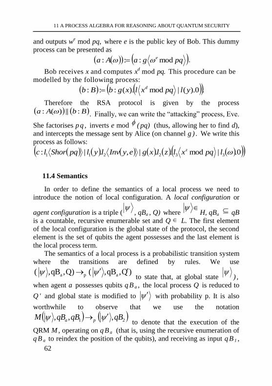
11 A PROCESS ALGEBRA FOR REASONING ABOUT QUANTUM SECURITY

62

and outputs we mod pq, where e is the public key of Bob. This dummy

process can be presented as

pqgaAa e mod::: .

Bob receives x and computes xd mod pq. This procedure can be

modelled by the following process:

.0).(|mod).(::: ylpqxlxgbBb d

Therefore the RSA protocol is given by the process

BbAa :||)(: . Finally, we can write the “attacking” process, Eve.

She factorises p q , inverts e mod ( pq) (thus, allowing her to find d),

and intercepts the message sent by Alice (on channel g ) . We write this

process as follows:

0.|mod..|,.|: 332211 lpqxlzlxgeyInvlylpqShorlc z

11.4 Semantics

In order to define the semantics of a local process we need to

introduce the notion of local configuration. A local configuration or

agent configuration is a triple (

, qBa , Q) where

H, qBa qB

is a countable, recursive enumerable set and Q L. The first element

of the local configuration is the global state of the protocol, the second

element is the set of qubits the agent possesses and the last element is

the local process term. The semantics of a local process is a probabilistic transition system

where the transitions are defined by rules. We use

)Q,qB, (Q),qB, ( apa

to state that, at global state

) ,

when agent a possesses qubits q B a , the local process Q is reduced to

Q ' and global state is modified to with probability p. It is also

worthwhile to observe that we use the notation

21 ,,, qBqBqBM pa to denote that the execution of the

QRM M , operating on q B a (that is, using the recursive enumeration of

q B a to reindex the position of the qubits), and receiving as input q B 1 ,

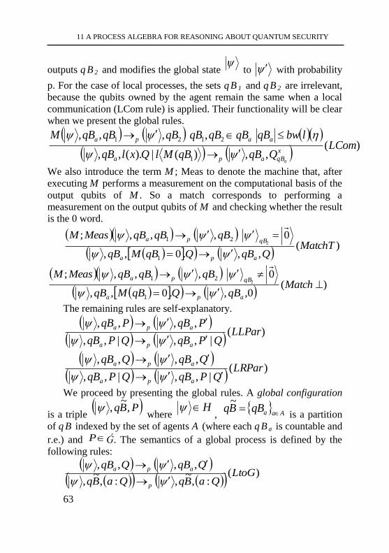
11 A PROCESS ALGEBRA FOR REASONING ABOUT QUANTUM SECURITY

63

outputs q B 2 and modifies the global state

to with probability

p. For the case of local processes, the sets q B 1 and q B 2 are irrelevant,

because the qubits owned by the agent remain the same when a local

communication (LCom rule) is applied. Their functionality will be clear

when we present the global rules.

)(

,,)(|).(,,

,,,,

1

2121LCom

QqBqBMlQxlqB

lbwqBqBqBqBqBqBqBM

x

qBapa

aapa

a

We also introduce the term M ; Meas to denote the machine that, after

executing M performs a measurement on the computational basis of the

output qubits of M . So a match corresponds to performing a

measurement on the output qubits of M and checking whether the result

is the 0 word.

)(

,,.0,,

0,,,;

1

212 MatchT

QqBQqBMqB

qBqBqBMeasM

apa

qBpa

)(

0,,.0,,

0,,,;

1

212

Match

qBQqBMqB

qBqBqBMeasM

apa

qBpa

The remaining rules are self-explanatory.

)(|,,|,,

,,,,LLPar

QPqBQPqB

PqBPqB

apa

apa

)(|,,|,,

,,,,LRPar

QPqBQPqB

QqBQqB

apa

apa

We proceed by presenting the global rules. A global configuration

is a triple PBq ,

~,

where H

,

AaaqBBq

~

is a partition

of q B indexed by the set of agents A (where each q B a is countable and

r.e.) and P Ǵ. The semantics of a global process is defined by the

following rules:

)(:,

~,:,

~,

,,,,LtoG

QaBqQaBq

QqBQqB

p

apa

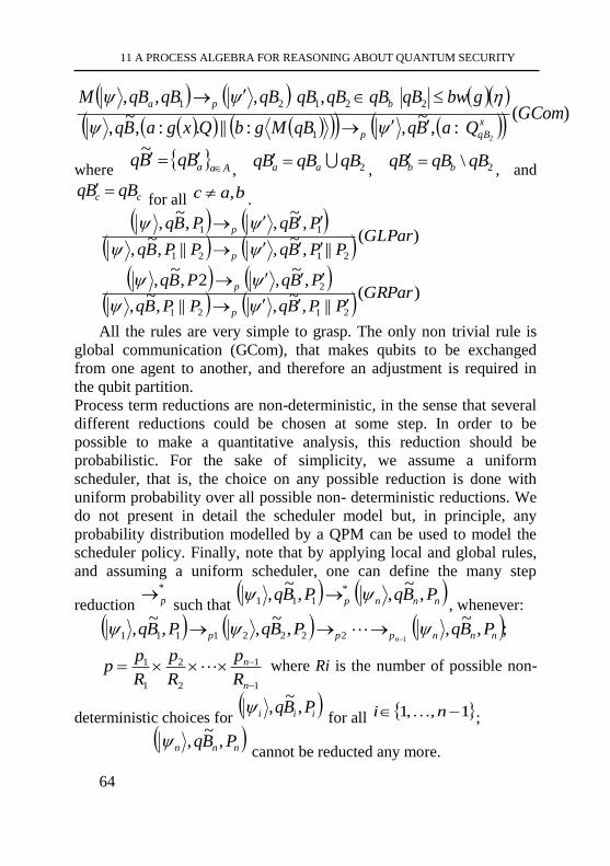
11 A PROCESS ALGEBRA FOR REASONING ABOUT QUANTUM SECURITY

64

)(

:,~

,:||.:,~

,

,,,,

21

22121GCom

QaBqqBMgbQxgaBq

gbwqBqBqBqBqBqBqBM

x

qBp

bpa

where

AaaBqBq

~

, 2qBqBBq aa , 2\ qBqBBq bb , and

cc qBBq for all bac , .

)(||,

~,||,

~,

,~

,,~

,

2121

11GLPar

PPBqPPBq

PBqPBq

p

p

)(||,

~,||,

~,

,~

,2,~

,

2121

2GRPar

PPBqPPBq

PBqPBq

p

p

All the rules are very simple to grasp. The only non trivial rule is

global communication (GCom), that makes qubits to be exchanged

from one agent to another, and therefore an adjustment is required in

the qubit partition.

Process term reductions are non-deterministic, in the sense that several

different reductions could be chosen at some step. In order to be

possible to make a quantitative analysis, this reduction should be

probabilistic. For the sake of simplicity, we assume a uniform

scheduler, that is, the choice on any possible reduction is done with

uniform probability over all possible non- deterministic reductions. We

do not present in detail the scheduler model but, in principle, any

probability distribution modelled by a QPM can be used to model the

scheduler policy. Finally, note that by applying local and global rules,

and assuming a uniform scheduler, one can define the many step

reduction

*

p such that

nnnp PBqPBq ,~

,,~

, *

111 , whenever:

;,~

,,~

,,~

,122221111 nnnppp PBqPBqPBq

n

1

1

2

2

1

1

n

n

R

p

R

p

R

pp where Ri is the number of possible non-

deterministic choices for iii PBq ,

~,

for all 1,,1 ni ;

nnn PBq ,~

, cannot be reducted any more.

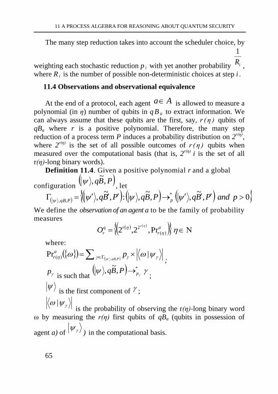
11 A PROCESS ALGEBRA FOR REASONING ABOUT QUANTUM SECURITY

65

The many step reduction takes into account the scheduler choice, by

weighting each stochastic reduction p i with yet another probability iR

1

,

where R i is the number of possible non-deterministic choices at step i .

11.4 Observations and observational equivalence

At the end of a protocol, each agent Aa is allowed to measure a

polynomial (in η) number of qubits in q B a to extract information. We

can always assume that these qubits are the first, say, r ( η ) qubits of

qBa where r is a positive polynomial. Therefore, the many step

reduction of a process term P induces a probability distribution on 2r(η)

,

where 2r(η)

is the set of all possible outcomes of r ( η ) qubits when

measured over the computational basis (that is, 2r(η)

i is the set of all

r(η)-long binary words).

Definition 11.4. Given a positive polynomial r and a global

configuration PBq ,

~,

, let

0,~

,,~

,:,~

, *

,, pandPBqPBqPBq pPqB

We define the observation of an agent a to be the family of probability

measures a

r

rq

r

r

O )(

2 Pr,2,2

where:

|Pr,,)( pPqB

a

r;

p is such that

*,~

, pPBq ;

is the first component of ;

| is the probability of observing the r(η)-long binary word

ω by measuring the r(η) first qubits of qBa (qubits in possession of

agent a) of ) in the computational basis.

11 A PROCESS ALGEBRA FOR REASONING ABOUT QUANTUM SECURITY

66

Note that the summation used to compute

a

r )(Pr is well

defined, since PqB,, is finite. It is clear at this point,that an

observation of an agent is a random r(η)-long binary word, with

distribution given by

a

r )(Pr .

The notion of observational equivalence we adopt is based on

computational indistinguishability as usual in the security community

[2]. First, we introduce the concept of context. The set of global

contexts C~

is defined inductively as follows: C~

; PC || and

CCP~

|| provided that CC~

and P Ǵ. Given a context

C and a global process P, the notation PC means that we

substitute the process P for the in C .

Definition 11.5. Let P and P' be process terms. We say that P is

computationally indistinguishable by agenl a from P' if and only if for

every context C , polynomials q and Hr ,

, partition Bq~

of

qB, η sufficiently large and binary word r2 ,

)(

1)(rP)(Pr )()(

q

a

r

a

r

where a

r )(Pr is given by the observation of a for configuration

PCBq ,~

, and

a

r )(rP is given by the observation of a for

configuration PCBq ,

~,

. In such case we write PP .

Two processes are computationally indistinguishable if they are

indistinguishable by contexts, that is, for any input (here modelled by

and Bq

~), there is no context which can distinguish, up to a

negligible function, the outputs produced. The definition above extends

the classical definition of computational indistinguishability to the

quantum case, since processes can be modelled by quantum polynomial

machines and therefore C induces the required distinguishing

11 A PROCESS ALGEBRA FOR REASONING ABOUT QUANTUM SECURITY

67

machine. A detailed proof of this result is out of the scope of this

extended abstract. In order to set up compositionality, the following

result is of the utmost importance:

Proposition 11.2. Computational indistinguishabilily is a

congruence relation with respecl to the parallel primitive of Ǵ.

Proof. Both symmetry and reflexivity are trivial to check.

Transitivity follows by triangular inequality, and taking into account

that )(

2

1nq

is a polynomial. Congruence on the global parallel operator

follows by noticing that for any contexts C and C , CC is

also a context. □

11.6 Emulation and Composition Theorem

One of the most successful ways for defining secure concurrent

cryptographic tasks is via process emulation [10, 11]. This definitional

job boils down to the following: a process realises a cryptographic task

if and only if it emulates an ideal process that is known to realise such

task. In this section, guided by the goal of defining secure

functionalities, we detail the notion of emulation for the quantum

process calculus defined in the previous section.

Let I be an ideal protocol that realises (the honest part of) some

secure protocol and P a process that implements the functionality

specified by I. The overall goal is to show that P realises, without

flaws, (part of) the secure functionality specified by I. The goal is

achieved if for any real adversary, say (a : A), the process P||(a : A) is

computationally indistinguishable by the adversary a from the process

I||(a : B) for some ideal adversary (a : B), where an ideal adversary is an

adversary which cannot corrupt I and a real adversary is any local

process for agent a. This property asserts that given a real adversary (a :

A), agent a cannot distinguish the information leaked by P||(a : A) from

the information leaked by the well behaved process I||(a : B) for some

ideal adversary (a : B), and therefore, we infer that P||(a : A) is also

well behaved. This discussion leads to the concept of emulation with

respect to a set of real adversaries A~

and ideal adversaries B~

.

11 A PROCESS ALGEBRA FOR REASONING ABOUT QUANTUM SECURITY

68

Definition 11.6. Let P and I be process terms and A~

and B~

sets of

global processes where the only agent is the adversary a, then P

emulates I with respect to A~

and B~

if and only if for all processes (a :

A) A~

there exists a process (a : B) B~

such that P||(a : A) ≈ I||(a :

B). In such case we write IP a

BA~

,~

and say that P is a secure

implementation of I with respect to A~

and B~

.

A desirable property of the emulation relation is the so called

Composition Theorem. This result was first discussed informally for

the classical secure computation setting in [12], and states the

following: if P is a secure implementation of part I of an ideal protocol,

R and J are two protocols which use the ideal protocol I as a

component, and finally, R is a secure implementation of J, then I

PR

should be a secure implementation of J. This result is captured as

follows:

Theorem 11.3. Let P,I be processes, R[ ] and J [ ] contexts and A~

,

B~

sets of processes over agent a and C~

, D~

sets of processes over

agent b. If ):(||):(|| ~

,~ BaIJBaIR b

DC

for any (a : B) B~

and

IP a

BA~

,~

then for any adversary (a : A) A~

there exists (a : B) B~

such that ):(||):(|| ~

,~ BaIJAaQR b

DC

.

Proof. Let (a : A) A~

and (a : B) B~

be such that

):(||):(|| BaIAaP . Now choose some (b : C) C~

, clearly,

):(||)]:(||[):(||)]:(||[ CcBaIRCcAaQR since ≈ is a congruence

relation. Moreover, since DCBaIR ~

,~)]:(||[

)]:(||[ BaIJ , there is a

(b : D) D~

such that ):(||)]:(||[||)]:(||[ DbBaIJCBaQR . Finally, by transitivity of ≈, we have that

):(||)]:(||[):(||)]:(||[ DbBaIJCbAaQR and hence

)]:(||[)]:(||[ ~,

~ BaIJAaQRDC

.

11 A PROCESS ALGEBRA FOR REASONING ABOUT QUANTUM SECURITY

69

Observe that ideal protocols are constituted by a honest part I and

an ideal adversary (a : B), and therefore are of the form I||(a : B). This

justifies why ):(|| BaIR was considered in the proposition above

instead of IR . Moreover, adversaries for the functionality

implemented by R and J might be different from those of I and Q,

therefore, two pairs of sets of processes C~

, D~

and A~

, B~

are required

to model two kinds of adversaries.

11.7 Quantum Zero-Knowledge Proofs

An interactive proof is a two party protocol, where one agent is

called the prover and the other is called the verifier. The main objective

of the protocol is to let the prover convince the verifier of the validity

of an assertion, however, this must be done in such a way that the

prover cannot convince the verifier of the validity of some false

assertion. Any interactive proof system fulfills two properties: completeness

and soundness. Completeness states that if the assertion the prover

wants to convince the verifier is true, then the verifier should be

convinced with probability one. On the other hand, soundness is

fulfilled if the verifier cannot be convinced, up to a negligible

probability, of a false assertion. Therefore, completeness and soundness

allow the verifier to check whether the assertion of the prover is true or

false. Zero-knowledge is a property of the prover (strategy). Consider the

following informal notion of (quantum) computational zero-knowledge

strategy, which corresponds to the straightforward lifting to the

quantum setting of the classical version: Definition 11.7. A prover strategy S is said to be quantum

computational zero-knowledge over a set L if and only if for every

quantum polynomial-time verifier strategy, V there exists quantum

polynomial-time algorithm M such that (S , V ) ( l ) is (quantum)

computationally indistinguishable from M (l ) for all l L, where (S ,

V ) denotes the output of the interaction between S and V. The main application of zero-knowledge proof protocols in the

cryptographic setting is in the context of a user U that has a secret and

is supposed to perform some steps, depending on the secret. The

11 A PROCESS ALGEBRA FOR REASONING ABOUT QUANTUM SECURITY

70

problem is how can other users assure that U has carried out the correct

steps without U disclosing its secret. Zero-knowledge proof protocols

(ZKP) can be used to satisfy these conflicting requirements.

Zero-knowledge essentially embodies that the verifier cannot gain

more knowledge when interacting with the prover than by running

alone a quantum polynomial time program (using the same input in

both cases). That is, running a the verifier in parallel with the prover

should be indistinguishable of some quantum polynomial time program. Actually, the notion of (quantum computational) zero-knowledge

proofs can be captured through emulation very easily. Assuming that a

proof strategy S(x) and verifier V(x) are modelled as terms of the

process algebra, it is actually possible to model the interaction between

p and v by the process (p : S) || (v : V). Denote by Lv (l) the set of all

process terms for the verifier x

lVv ):(, that is, any process term (v : V)

where the free variable x was replaced by the binary word l. We have

the following characterisation: Proposition 11.4. A process term (p : S) denoting a proof strategy

is compulational zero- knowledge for L if and only if

0):()(),(

v

lLlL

x

l vvSp , for all Ll .

Proof. Proof (Sketch): Notice that the ZKP resumes to impose that

for all x

lVv ):( there is a process

x

lVv ):( such that

x

l

x

l

x

l VvVvSp ):(||0):(||):( . Since the semantics of a local process

can be modelled by a QPM, and moreover x

lVv ):(||0 can model any

QPM, the characterisation proposed in this proposition is equivalent to

Definition 11.7. So, a process (p : S) models a quantum zero-knowledge strategy if,

from the point of view of the verifier, it is impossible to distinguish the

final result of the interaction with (p : S) from the interaction with the 0

process. A clear corollary of Theorem 11.3 is that, quantum zero-

knowledge is compositional. It is simple to adapt the emulation approach to several other

quantum security properties, like quantum secure computation,

authentication and so on.

11 A PROCESS ALGEBRA FOR REASONING ABOUT QUANTUM SECURITY

71

Advancement questions

1. What is the role of security parameters?

2. 0 Ǵ (global termination) ;

P|| (a : Q) Ǵ where P Ǵ, aA does not occur in P,

and QL (global parallel composition).

What does the following example describe?

3. What we need to introduce for order in order to define the

semantics of a local process?

4. What is the base of the semantcis of a local process?

5. What can be used to model the scheduler policy

6. What does global communication rule make?

2. What is the base of the notion of observational equivalence?

3. What the most successful ways for defining secure concurrent

cryptographic tasks?

4. How we can called the agents of a two party protocol?

5. What the main application of zero-knowledge proof protocols

in the cryptographic setting

REFERENCES

[1] Pedro Miguel dos Santos Alves Madeira Adão Formal

Methods for the Analysis of Security Protocols / Pedro Miguel dos

Santos Alves Madeira Adão // PhD diss., INSTITUTO SUPERIOR

TĖCNICO. – 2006.

[2] Mitchell J. C. A probabilistic polynomial-time calculus for

the analysis of cryptographic protocols / J. C. Mitchell, A. Ramanathan,

A. Scedrov, V. Teague //Electronic Notes in Theoretical Computer

Science. - 2001. - №45. - p. 1–31.

[3] Mateus P. Composition of cryptographic protocols in a

probabilistic polynomial-time process calculus / editors R. Amadio and

D. Lugiez. - Concurrency Theory. - 2003. - Vol2761. - p. 327–349.-

523 p.

11 A PROCESS ALGEBRA FOR REASONING ABOUT QUANTUM SECURITY

72

[4] Cook S. A. Time bounded random access machines / S. A.

Cook and R. A. Reckhow //Journal of Computer and System Sciences. -

1973. - Vol7. - p. 354–375.

[5] Knill E. Conventions for quantum pseudocode : Technical

Report LAUR-96-2724 / E. Knill. - Los Alamos : National Laboratory,

1996. - 13 p.

[6] Mateus P. Reasoning about quantum systems / editors J. J.

Alferes, J. A. Leite . - Proceedings of the 9th European Conference on

Logics in Artificial Intelligence (JELIA), 2004. - Vol3229. - p.239–

251. - 743p.

[7] Mateus P. Weakly complete axiomatization of exogenous

quantum propositional logic / P. Mateus, A. Sernadas // Information

and Computation. - 2006. - Vol204(5). - p. 771–794.

[8] Cohen-Tannoudji C. Quantum Mechanics / C. Cohen-

Tannoudji, B. Diu, and F. Laloë. - John Wiley, 1977. - 887 p.

[9] Martins A. M. Minimization of quantum automata / A. M.

Martins, P. Mateus, A. Sernadas // Technical report, CLC, Department

of Mathematics, Instituto Superior Técnico. - 2005. - 308p.

[10] Abadi M. A calculus for cryptographic protocols: The Spi

Calculus. Information and Computation / M. Abadi A. D. Gordon //

SRC Research Report 149. - 1999. - Vol148(1). - p.1–70.

[11] Canetti R. Security and composition of multiparty

cryptographic protocols / R. Canetti // Journal of Cryptology. - 2000. -

Vol13(1). - p.143–202.

[12] Micali S. Secure computation / S. Micali, P. Rogaway // In

Feigenbaum. - 2000. - p. 392–404.

12 INTELLECTUAL METHODS FOR SECURITY

73

CHAPTER 12. INTELLECTUAL METHODS FOR

SECURITY

Content of the PART3

GLOSSARY ........................... Ошибка! Закладка не определена.

PART 3. Formal and Intellectual Methods for System Security and

Resilience ............................... Ошибка! Закладка не определена.

Content of the PART3 ............ Ошибка! Закладка не определена.

CHAPTER 10. Process Algebras for Studying Security ..... Ошибка!

Закладка не определена.

Content of the CHAPTER 10 . Ошибка! Закладка не определена.

Introduction ............................ Ошибка! Закладка не определена.

10.1 Low-Level Target Model Ошибка! Закладка не определена.

10.2 A Distributed Calculus with Principals and Authentica-tionОшибка! Закладка не определена.

Syntax and Informal SemanticsОшибка! Закладка не определена.

Operational Semantics ............ Ошибка! Закладка не определена.

Local Reductions .................... Ошибка! Закладка не определена.

System Transitions ................. Ошибка! Закладка не определена.

Compositionality .................... Ошибка! Закладка не определена.

An Abstract Machine for Local ReductionsОшибка! Закладка не определена.

10.3 High-Level Equivalences and SafetyОшибка! Закладка не определена.

Bounding processes ................ Ошибка! Закладка не определена.

Equivalences with Message Authentication; Strong Secrecy and

Authentication ........................ Ошибка! Закладка не определена.

Equivalences with Certificates Ошибка! Закладка не определена.

10.4 Applications .................... Ошибка! Закладка не определена.

12 INTELLECTUAL METHODS FOR SECURITY

74

Anonymous Forwarders ......... Ошибка! Закладка не определена.

Electronic Payment Protocol .. Ошибка! Закладка не определена.

Initialisation ............................ Ошибка! Закладка не определена.

10.5 A Concrete ImplementationОшибка! Закладка не определена.

Implementation of Machines .. Ошибка! Закладка не определена.

Low-level Processes ReductionsОшибка! Закладка не определена.

Marshaling and Unmarshaling ProtocolsОшибка! Закладка не определена.

Sending and Receiving ProtocolsОшибка! Закладка не определена.

Mapping High-Level Systems to Low-Level MachinesОшибка! Закладка не определена.

10.11 Main Results ................. Ошибка! Закладка не определена.

chapter 11. A Process Algebra for Reasoning About Quantum Security

Ошибка! Закладка не определена.

Introduction ............................ Ошибка! Закладка не определена.

11.1 Process Algebra .............. Ошибка! Закладка не определена.

11.2 Quantum polynomial machinesОшибка! Закладка не определена.

11.3 Process algebra ............... Ошибка! Закладка не определена.

11.4 Semantics ........................ Ошибка! Закладка не определена.

11.4 Observations and observational equivalenceОшибка! Закладка не определена.

11.6 Emulation and Composition TheoremОшибка! Закладка не определена.

11.7 Quantum Zero-Knowledge ProofsОшибка! Закладка не определена.

chapter 12. Intellectual methods for securityОшибка! Закладка не

определена.

12.1 Application of Artificial Intelligence in Network Intrusion

Detection ................................. Ошибка! Закладка не определена.

Background Knowledge ......... Ошибка! Закладка не определена.

12 INTELLECTUAL METHODS FOR SECURITY

75

Overview of Some Artificial Intelligence Techniques and their

Application in IDS .................. Ошибка! Закладка не определена.

Advances in Artificial Intelligence Hybrid and Ensemble

Techniques in IDS .................. Ошибка! Закладка не определена.

12.2 Multi-agent based approach of botnet detection in computer

systems ................................... Ошибка! Закладка не определена.

Multi-agent system of botnet detectionОшибка! Закладка не определена.

Sensor of botnet detection in monitor modeОшибка! Закладка не определена.

Sensor of botnet detection in scanner modeОшибка! Закладка не определена.

Agents’ functioning ................ Ошибка! Закладка не определена.

Experiments ............................ Ошибка! Закладка не определена.

12.3 Technique for bots detection which use polymorphic codeОшибка! Закладка не определена.

Related works ......................... Ошибка! Закладка не определена.

Previous work ......................... Ошибка! Закладка не определена.

Technique for bots detection which use polymorphic codeОшибка! Закладка не определена.

Levels of polymorphism ......... Ошибка! Закладка не определена.

The first level of polymorphismОшибка! Закладка не определена.

The second level of polymorphismОшибка! Закладка не определена.

The third/fourth levels of polymorphismОшибка! Закладка не определена.

The fifth level of polymorphismОшибка! Закладка не определена.

The sixth level of polymorphismОшибка! Закладка не определена.

Polymorhic code detection sensorОшибка! Закладка не определена.

Experiments ............................ Ошибка! Закладка не определена.

Conclusions ............................ Ошибка! Закладка не определена.

12 INTELLECTUAL METHODS FOR SECURITY

76

chapter 13. Methods and Techniques for Formal Development and

Quantitative Assessment. Resilient systemsОшибка! Закладка не

определена.

Background: Concepts ............ Ошибка! Закладка не определена.

Resilience Concept ................. Ошибка! Закладка не определена.

Dependability: Basic DefinitionsОшибка! Закладка не определена.

Goal-Based Development ....... Ошибка! Закладка не определена.

System Autonomy and ReconfigurationОшибка! Закладка не определена.

Methods and Techniques for Formal Development and Quantitative

Assessment ............................. Ошибка! Закладка не определена.

Development Methodologies .. Ошибка! Закладка не определена.

Event-B Method ..................... Ошибка! Закладка не определена.

Quantitative Assessment......... Ошибка! Закладка не определена.

PRISM model checker ............ Ошибка! Закладка не определена.

Discrete-event simulation ....... Ошибка! Закладка не определена.

CHAPTER 14. Formal Development and Quantitative Assessment of

Resilient Distributed Systems . Ошибка! Закладка не определена.

14.1 Overview of the Proposed ApproachОшибка! Закладка не определена.

14.2 Resilience-Explicit Development Based on Functional

Decomposition. ....................... Ошибка! Закладка не определена.

14.3 Modelling Component Interactions with Multi-Agent

Framework .............................. Ошибка! Закладка не определена.

14.4 Goal-Oriented Modelling of Resilient SystemsОшибка! Закладка не определена.

14.5 Pattern-Based Formal Development of Resilient MASОшибка! Закладка не определена.

14.6 Formal Goal-Oriented Reasoning About Resilient Re-

configurable MAS .................. Ошибка! Закладка не определена.

12 INTELLECTUAL METHODS FOR SECURITY

77

14.7 Modelling and Assessment of Resilient ArchitecturesОшибка! Закладка не определена.

12 INTELLECTUAL METHODS FOR SECURITY

78

12.1 Application of Artificial Intelligence in Network Intrusion

Detection

Introduction

Intrusion Detection System (IDS) is the process of monitoring the

events occurring in a computer system or network and analyzing them

for signs of intrusion [1,2]. It is useful not only in detecting successful

intrusions, but also in monitoring attempts to break security, which

provides important information for timely counter-measures. Basically,

IDS can be classified into two types: Misuse Intrusion Detection and

Anomaly Intrusion Detection. Traditional protection techniques such as

user authentication, data encryption, avoiding programming errors, and

firewalls are used as first lines of defense for computer security. If a

weak password is compromised, user authentication cannot prevent

unauthorized use. Also, firewalls are vulnerable to errors in

configuration and susceptible to ambiguous or undefined security

policies.

Recently, the use of Artificial Intelligence (AI) techniques has been

employed in different data mining and machine learning classification

and prediction modeling schemes. In addition to these, hybrid data

mining schemes, hierarchical hybrid intelligent system models, and

ensemble learning approaches that combine the base models with other

hybrid machine learning paradigms, to maximize the accuracy and

minimize both root mean squared errors and computational complexity,

have also gained popularity in the literature [3].

In this chapter, a succinct review has been carried out on the

individual capabilities of various AI techniques in their application to

network IDS. Such techniques include Artificial Neural Networks

(ANN), Support Vector Machines (SVM), Genetic Algorithms (GA)

and Fuzzy Neural Networks (FNN). Attempts were also made to

propose possible hybrid approaches based on these techniques.

Background Knowledge

Overview of Intrusion Detection Systems Intrusion Detection Systems are used to monitor computers or

networks for unauthorized entrance or activities, thereby making it easy

12 INTELLECTUAL METHODS FOR SECURITY

79

to detect if a system is being targeted by an attack. Preventing,

detecting, and reacting to intrusions without disturbing the operations

of existing systems remain a big challenge for networks that provide

round the clock services such as web servers. In such networks, even if

an intrusion is detected, the system cannot be shut down to check it

fully since it may be serving users who are making deals or completing

one transaction or the other [2]. An IDS inspects all inbound and outbound network activity and

identifies suspicious patterns that may indicate a network or system

attack from someone attempting to break into or compromise a system.

Generally, an IDS detects unwanted manipulations of computer

systems, mainly through the Internet. The manipulations may take the

form of attacks by crackers [4]. An IDS is composed of three major components: Sensors which

generate security events, a Console to monitor events, initiate alerts and

control the sensors, and a Central Engine that records events logged by

the sensors in a database and uses a system of rules to generate alerts

from security events that have been received [5]. There are three major categories of IDS viz. Misuse Detection vs.

Anomaly Detection, Network-Based vs. Host- Based Systems and

Passive System vs. Reactive System. Misuse Detection vs. Anomaly Detection: The Misuse Detection part analyses the information it gathers, and

compares it to large databases of attack signatures by looking for a

specific attack that has already been documented while the Anomaly

Detection part monitors network segments to compare their state to the

normal baseline defined by the systems administrator and look for

anomalies [6]. Network-Based vs. Host-Based Systems: In the Network-based system, the network analyses individual

packets of information flowing through it and detects those that are

malicious but designed to be overlooked by a firewall’s simplistic

filtering rules. In a Host- based system, the IDS examines the activity

on each individual computer or host [6]. Passive System vs. Reactive System: In a Passive System, the IDS detects a potential security breach,

logs the information and raises an alert signal while the reactive system

12 INTELLECTUAL METHODS FOR SECURITY

80

responds to the suspicious activity by logging off a user or by

reprogramming the firewall to block network traffic from the suspected

malicious source [6]. Overview of Artificial Intelligence The application of the capabilities of Artificial Intelligence

techniques has been widely appreciated in Computer and

Communication Networks in particular, as well as in other fields. This

inter-disciplinary endeavor has created a collaborative link between

Computer Scientists and Network Engineers in the design, simulation

and development of network intrusion models and their characteristics.

Computational Intelligence (CI), an offshoot of AI, covers all branches

of science and engineering that are concerned with the understanding

and solving of problems for which effective computational algorithms

do not yet exist. Thus, it overlaps with some areas of Artificial

Intelligence and a good part of Pattern Recognition, Image Analysis

and Operations Research. It is based on the assumption that thinking is

nothing but symbol manipulation. Thus, it holds out the hope that

computers will not merely simulate intelligence, but actually achieve it.

CI relies on heuristic algorithms such as in Fuzzy Systems, Neural

Networks, Support Vector Machines and Evolutionary Computation. In

addition, CI also embraces techniques that use Swarm Intelligence,

Fractals and Chaos Theory, Artificial Immune Systems, Wavelets, etc.

[7].

AI is itself an advancement of the concept of its predecessor, Data

Mining (DM). DM is the process of finding previously unknown,

profitable and useful patterns embedded in data, with no prior

hypothesis. It is the process of analyzing data from different

perspectives, summarizing it into useful information and finding

correlations or patterns among datasets in large data repositories. The

objective of DM is to use the discovered patterns to help explain

current behavior or to predict future outcomes. DM borrows some

concepts and techniques from several long-established disciplines viz.

Artificial Intelligence, Database Technology, Machine Learning and

Statistics. The field of DM has, over the past couple of decades,

produced a rich variety of algorithms that enable computers to learn

new relationships/knowledge from large datasets [8].

12 INTELLECTUAL METHODS FOR SECURITY

81

AI naturally transformed into Computational Intelligence (CI) with

the introduction of the concept of Machine Learning. This is a scientific

aspect of AI that is concerned with the design and development of

algorithms that allow computers to learn based on data, such as a

network intrusion log acquired over a considerable period of time. A

major focus of machine learning research is to automatically learn to

recognize complex attributes and to make intelligent decisions based on

the correlations among the data variables. Hence, machine learning is

closely related to fields such as statistics, probability theory, data

mining, pattern recognition, artificial intelligence, adaptive control, and

theoretical computer science.

The machine learning concept can be categorized into three

common algorithms viz. supervised, unsupervised and hybrid learning.

Supervised learning is the type of machine learning technique in which

the algorithm generates a function that maps inputs to the desired

outputs with the least possible error. Unsupervised learning is the

machine learning technique in which a set of inputs are analyzed

without the target output. This is also called clustering. The hybrid

learning combines the supervised and unsupervised techniques to

generate an appropriate function and to meet a specific need of solving

a problem. The computational analysis of machine learning algorithms

and their performance is a branch of theoretical computer science

known as computational learning theory [8].

A general modeling framework for computational intelligence is

shown Figure 12.1.

12 INTELLECTUAL METHODS FOR SECURITY

82

Figure 12.1. Computational Intelligence Modeling Framework

Overview of Some Artificial Intelligence Techniques and their

Application in IDS

A good number of studies have been carried out on the use of

various CI/AI techniques to model various IDS strategies. Some of

these techniques will be discussed in the following sections. Artificial Neural Networks (ANN) Attempts to artificially simulate the biological processes that lead to

intelligent behavior culminated in the development of ANN. ANN is a

mathematical or computational model that is based on biological neural

networks. It consists of an interconnected group of artificial neurons

which processes information using a connectionist approach to

computation. In most cases, ANN is an adaptive system that changes its

structure based on external or internal information that flows through

the network during the learning phase. In more practical terms, neural networks are non-linear statistical

data modeling tools. They can be used to model complex relationships

between inputs and outputs or to find patterns in data. A typical ANN

framework is shown in figure 12.2 ANN is a close emulation of the

biological nervous system. In this model, a neuron multiplies the inputs

by weights, calculates the sum, and applies a threshold. The result of

this computation would then be transmitted to subsequent neurons.

Basically, the ANN has been generalized to:

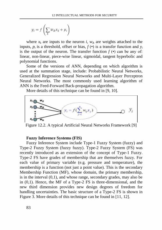
12 INTELLECTUAL METHODS FOR SECURITY

83

where xk are inputs to the neuron i, wlk are weights attached to the

inputs, pt is a threshold, offset or bias, f (•) is a transfer function and yi

is the output of the neuron. The transfer function f (•) can be any of:

linear, non-linear, piece-wise linear, sigmoidal, tangent hyperbolic and

polynomial functions. Some of the versions of ANN, depending on which algorithm is

used at the summation stage, include: Probabilistic Neural Networks,

Generalized Regression Neural Networks and Multi-Layer Perceptron

Neural Networks. The most commonly used learning algorithm of

ANN is the Feed-Forward Back-propagation algorithm.

More details of this technique can be found in [9, 10].

Figure 12.2. A typical Artificial Neural Networks Framework [9]

Fuzzy Inference Systems (FIS)

Fuzzy Inference System include Type-1 Fuzzy System (fuzzy) and

Type-2 Fuzzy System (fuzzy fuzzy). Type-2 Fuzzy System (FS) was

recently introduced as an extension of the concept of Type-1 Fuzzy.

Type-2 FS have grades of membership that are themselves fuzzy. For

each value of primary variable (e.g. pressure and temperature), the

membership is a function (not just a point value). This is the secondary

Membership Function (MF), whose domain, the primary membership,

is in the interval (0,1), and whose range, secondary grades, may also be

in (0,1). Hence, the MF of a Type-2 FS is three-dimensional, and the

new third dimension provides new design degrees of freedom for

handling uncertainties. The basic structure of a Type-2 FS is shown in

Figure 3. More details of this technique can be found in [11, 12].

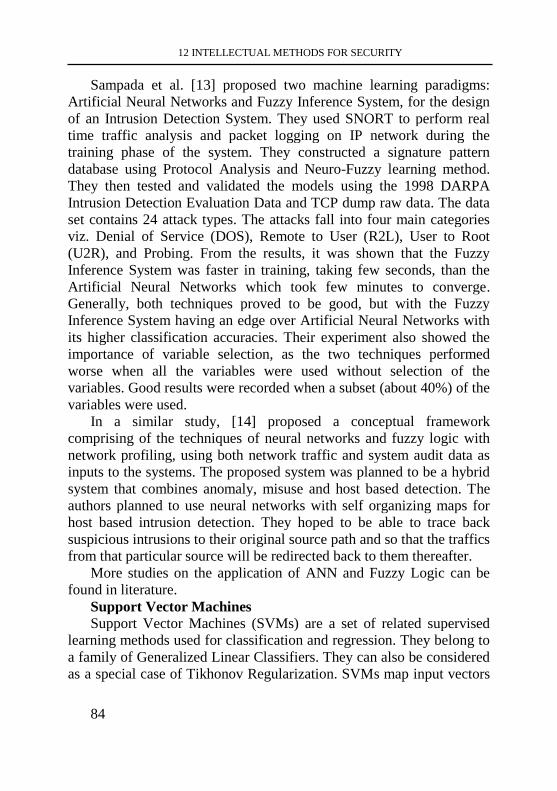
12 INTELLECTUAL METHODS FOR SECURITY

84

Sampada et al. [13] proposed two machine learning paradigms:

Artificial Neural Networks and Fuzzy Inference System, for the design

of an Intrusion Detection System. They used SNORT to perform real

time traffic analysis and packet logging on IP network during the

training phase of the system. They constructed a signature pattern

database using Protocol Analysis and Neuro-Fuzzy learning method.

They then tested and validated the models using the 1998 DARPA

Intrusion Detection Evaluation Data and TCP dump raw data. The data

set contains 24 attack types. The attacks fall into four main categories

viz. Denial of Service (DOS), Remote to User (R2L), User to Root

(U2R), and Probing. From the results, it was shown that the Fuzzy

Inference System was faster in training, taking few seconds, than the

Artificial Neural Networks which took few minutes to converge.

Generally, both techniques proved to be good, but with the Fuzzy

Inference System having an edge over Artificial Neural Networks with

its higher classification accuracies. Their experiment also showed the

importance of variable selection, as the two techniques performed

worse when all the variables were used without selection of the

variables. Good results were recorded when a subset (about 40%) of the

variables were used. In a similar study, [14] proposed a conceptual framework

comprising of the techniques of neural networks and fuzzy logic with

network profiling, using both network traffic and system audit data as

inputs to the systems. The proposed system was planned to be a hybrid

system that combines anomaly, misuse and host based detection. The

authors planned to use neural networks with self organizing maps for

host based intrusion detection. They hoped to be able to trace back

suspicious intrusions to their original source path and so that the traffics

from that particular source will be redirected back to them thereafter. More studies on the application of ANN and Fuzzy Logic can be

found in literature. Support Vector Machines Support Vector Machines (SVMs) are a set of related supervised

learning methods used for classification and regression. They belong to

a family of Generalized Linear Classifiers. They can also be considered

as a special case of Tikhonov Regularization. SVMs map input vectors

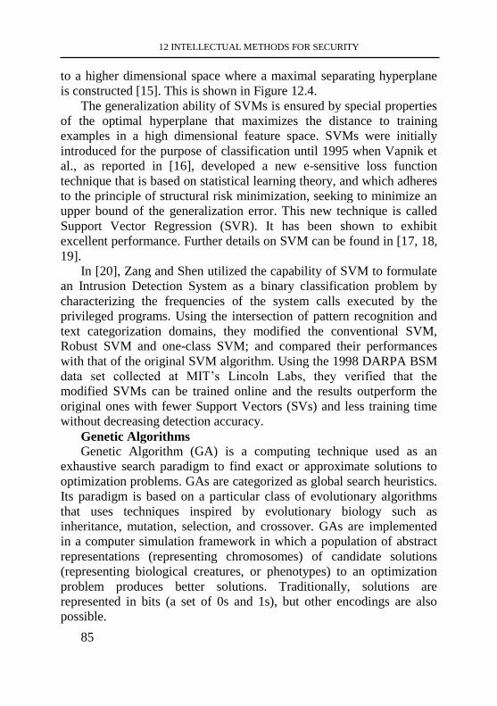
12 INTELLECTUAL METHODS FOR SECURITY

85

to a higher dimensional space where a maximal separating hyperplane

is constructed [15]. This is shown in Figure 12.4. The generalization ability of SVMs is ensured by special properties

of the optimal hyperplane that maximizes the distance to training

examples in a high dimensional feature space. SVMs were initially

introduced for the purpose of classification until 1995 when Vapnik et

al., as reported in [16], developed a new e-sensitive loss function

technique that is based on statistical learning theory, and which adheres

to the principle of structural risk minimization, seeking to minimize an

upper bound of the generalization error. This new technique is called

Support Vector Regression (SVR). It has been shown to exhibit

excellent performance. Further details on SVM can be found in [17, 18,

19]. In [20], Zang and Shen utilized the capability of SVM to formulate

an Intrusion Detection System as a binary classification problem by

characterizing the frequencies of the system calls executed by the

privileged programs. Using the intersection of pattern recognition and

text categorization domains, they modified the conventional SVM,

Robust SVM and one-class SVM; and compared their performances

with that of the original SVM algorithm. Using the 1998 DARPA BSM

data set collected at MIT’s Lincoln Labs, they verified that the

modified SVMs can be trained online and the results outperform the

original ones with fewer Support Vectors (SVs) and less training time

without decreasing detection accuracy.

Genetic Algorithms

Genetic Algorithm (GA) is a computing technique used as an

exhaustive search paradigm to find exact or approximate solutions to

optimization problems. GAs are categorized as global search heuristics.

Its paradigm is based on a particular class of evolutionary algorithms

that uses techniques inspired by evolutionary biology such as

inheritance, mutation, selection, and crossover. GAs are implemented

in a computer simulation framework in which a population of abstract

representations (representing chromosomes) of candidate solutions

(representing biological creatures, or phenotypes) to an optimization

problem produces better solutions. Traditionally, solutions are

represented in bits (a set of 0s and 1s), but other encodings are also

possible.

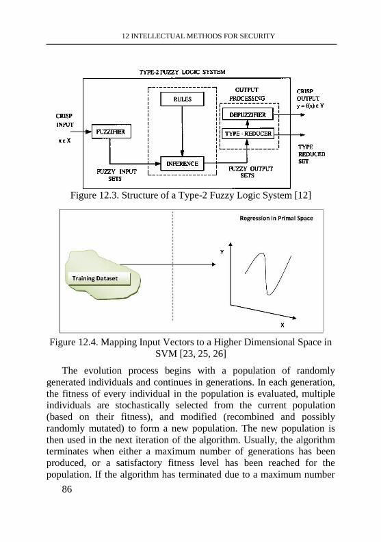
12 INTELLECTUAL METHODS FOR SECURITY

86

Figure 12.3. Structure of a Type-2 Fuzzy Logic System [12]

Figure 12.4. Mapping Input Vectors to a Higher Dimensional Space in

SVM [23, 25, 26]

The evolution process begins with a population of randomly

generated individuals and continues in generations. In each generation,

the fitness of every individual in the population is evaluated, multiple

individuals are stochastically selected from the current population

(based on their fitness), and modified (recombined and possibly

randomly mutated) to form a new population. The new population is

then used in the next iteration of the algorithm. Usually, the algorithm

terminates when either a maximum number of generations has been

produced, or a satisfactory fitness level has been reached for the

population. If the algorithm has terminated due to a maximum number

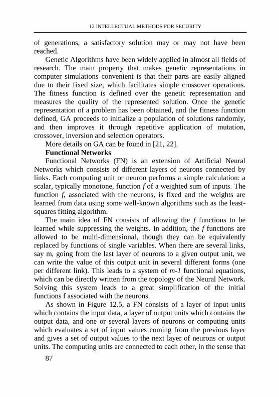
12 INTELLECTUAL METHODS FOR SECURITY

87

of generations, a satisfactory solution may or may not have been

reached. Genetic Algorithms have been widely applied in almost all fields of

research. The main property that makes genetic representations in

computer simulations convenient is that their parts are easily aligned

due to their fixed size, which facilitates simple crossover operations.

The fitness function is defined over the genetic representation and

measures the quality of the represented solution. Once the genetic

representation of a problem has been obtained, and the fitness function

defined, GA proceeds to initialize a population of solutions randomly,

and then improves it through repetitive application of mutation,

crossover, inversion and selection operators. More details on GA can be found in [21, 22]. Functional Networks Functional Networks (FN) is an extension of Artificial Neural

Networks which consists of different layers of neurons connected by

links. Each computing unit or neuron performs a simple calculation: a

scalar, typically monotone, function f of a weighted sum of inputs. The

function f, associated with the neurons, is fixed and the weights are

learned from data using some well-known algorithms such as the least-

squares fitting algorithm. The main idea of FN consists of allowing the f functions to be

learned while suppressing the weights. In addition, the f functions are

allowed to be multi-dimensional, though they can be equivalently

replaced by functions of single variables. When there are several links,

say m, going from the last layer of neurons to a given output unit, we

can write the value of this output unit in several different forms (one

per different link). This leads to a system of m-1 functional equations,

which can be directly written from the topology of the Neural Network.

Solving this system leads to a great simplification of the initial

functions f associated with the neurons. As shown in Figure 12.5, a FN consists of a layer of input units

which contains the input data, a layer of output units which contains the

output data, and one or several layers of neurons or computing units

which evaluates a set of input values coming from the previous layer

and gives a set of output values to the next layer of neurons or output

units. The computing units are connected to each other, in the sense that

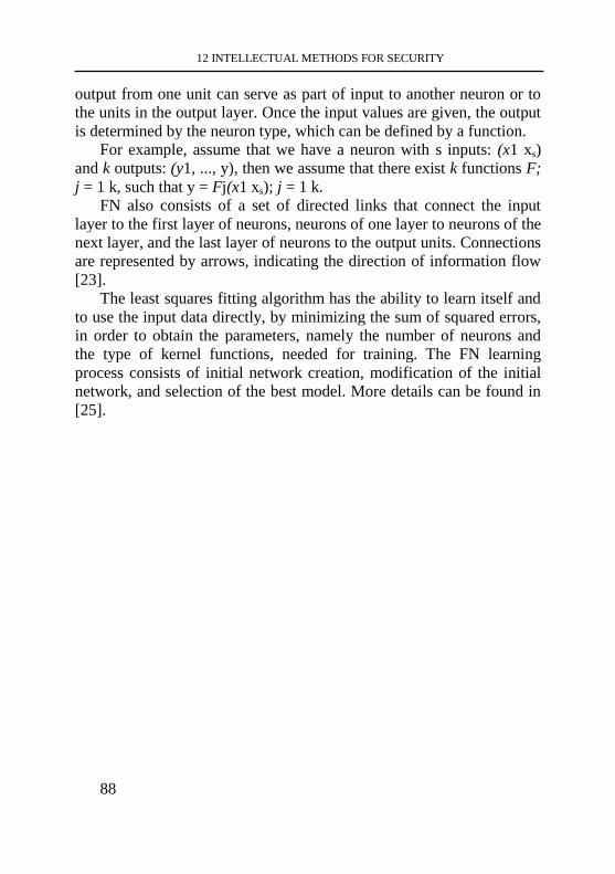
12 INTELLECTUAL METHODS FOR SECURITY

88

output from one unit can serve as part of input to another neuron or to

the units in the output layer. Once the input values are given, the output

is determined by the neuron type, which can be defined by a function.

For example, assume that we have a neuron with s inputs: (x1 xs)

and k outputs: (y1, ..., y), then we assume that there exist k functions F;

j = 1 k, such that y = Fj(x1 xs); j = 1 k.

FN also consists of a set of directed links that connect the input

layer to the first layer of neurons, neurons of one layer to neurons of the

next layer, and the last layer of neurons to the output units. Connections

are represented by arrows, indicating the direction of information flow

[23].

The least squares fitting algorithm has the ability to learn itself and

to use the input data directly, by minimizing the sum of squared errors,

in order to obtain the parameters, namely the number of neurons and

the type of kernel functions, needed for training. The FN learning

process consists of initial network creation, modification of the initial

network, and selection of the best model. More details can be found in

[25].

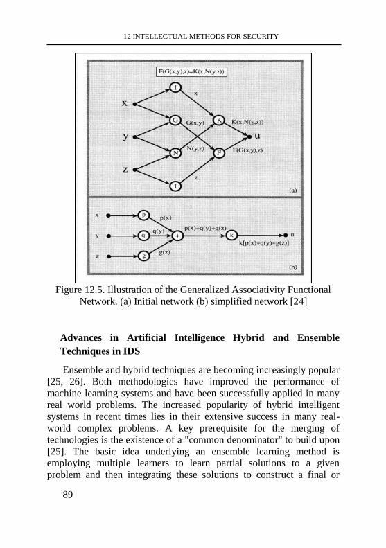
12 INTELLECTUAL METHODS FOR SECURITY

89

Figure 12.5. Illustration of the Generalized Associativity Functional

Network. (a) Initial network (b) simplified network [24]

Advances in Artificial Intelligence Hybrid and Ensemble

Techniques in IDS

Ensemble and hybrid techniques are becoming increasingly popular

[25, 26]. Both methodologies have improved the performance of

machine learning systems and have been successfully applied in many

real world problems. The increased popularity of hybrid intelligent

systems in recent times lies in their extensive success in many real-

world complex problems. A key prerequisite for the merging of

technologies is the existence of a "common denominator" to build upon

[25]. The basic idea underlying an ensemble learning method is

employing multiple learners to learn partial solutions to a given

problem and then integrating these solutions to construct a final or

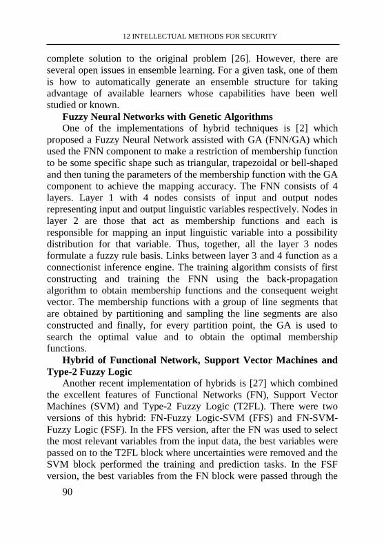
12 INTELLECTUAL METHODS FOR SECURITY

90

complete solution to the original problem [26]. However, there are

several open issues in ensemble learning. For a given task, one of them

is how to automatically generate an ensemble structure for taking

advantage of available learners whose capabilities have been well

studied or known.

Fuzzy Neural Networks with Genetic Algorithms One of the implementations of hybrid techniques is [2] which

proposed a Fuzzy Neural Network assisted with GA (FNN/GA) which

used the FNN component to make a restriction of membership function

to be some specific shape such as triangular, trapezoidal or bell-shaped

and then tuning the parameters of the membership function with the GA

component to achieve the mapping accuracy. The FNN consists of 4

layers. Layer 1 with 4 nodes consists of input and output nodes

representing input and output linguistic variables respectively. Nodes in

layer 2 are those that act as membership functions and each is

responsible for mapping an input linguistic variable into a possibility

distribution for that variable. Thus, together, all the layer 3 nodes

formulate a fuzzy rule basis. Links between layer 3 and 4 function as a

connectionist inference engine. The training algorithm consists of first

constructing and training the FNN using the back-propagation

algorithm to obtain membership functions and the consequent weight

vector. The membership functions with a group of line segments that

are obtained by partitioning and sampling the line segments are also

constructed and finally, for every partition point, the GA is used to

search the optimal value and to obtain the optimal membership

functions. Hybrid of Functional Network, Support Vector Machines and

Type-2 Fuzzy Logic Another recent implementation of hybrids is [27] which combined

the excellent features of Functional Networks (FN), Support Vector

Machines (SVM) and Type-2 Fuzzy Logic (T2FL). There were two

versions of this hybrid: FN-Fuzzy Logic-SVM (FFS) and FN-SVM-

Fuzzy Logic (FSF). In the FFS version, after the FN was used to select

the most relevant variables from the input data, the best variables were

passed on to the T2FL block where uncertainties were removed and the

SVM block performed the training and prediction tasks. In the FSF

version, the best variables from the FN block were passed through the

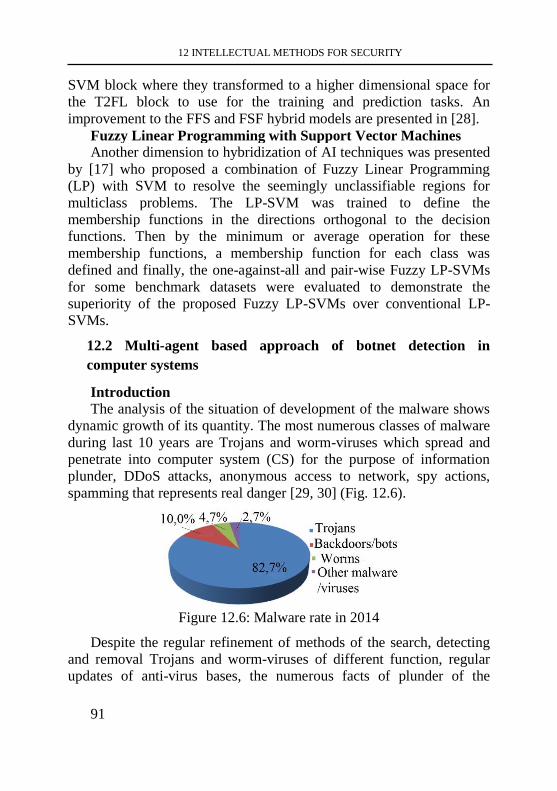
12 INTELLECTUAL METHODS FOR SECURITY

91

SVM block where they transformed to a higher dimensional space for

the T2FL block to use for the training and prediction tasks. An

improvement to the FFS and FSF hybrid models are presented in [28]. Fuzzy Linear Programming with Support Vector Machines Another dimension to hybridization of AI techniques was presented

by [17] who proposed a combination of Fuzzy Linear Programming

(LP) with SVM to resolve the seemingly unclassifiable regions for

multiclass problems. The LP-SVM was trained to define the

membership functions in the directions orthogonal to the decision

functions. Then by the minimum or average operation for these

membership functions, a membership function for each class was

defined and finally, the one-against-all and pair-wise Fuzzy LP-SVMs

for some benchmark datasets were evaluated to demonstrate the

superiority of the proposed Fuzzy LP-SVMs over conventional LP-

SVMs.

12.2 Multi-agent based approach of botnet detection in

computer systems

Introduction

The analysis of the situation of development of the malware shows

dynamic growth of its quantity. The most numerous classes of malware

during last 10 years are Trojans and worm-viruses which spread and

penetrate into computer system (CS) for the purpose of information

plunder, DDoS attacks, anonymous access to network, spy actions,

spamming that represents real danger [29, 30] (Fig. 12.6).

Figure 12.6: Malware rate in 2014

Despite the regular refinement of methods of the search, detecting

and removal Trojans and worm-viruses of different function, regular

updates of anti-virus bases, the numerous facts of plunder of the

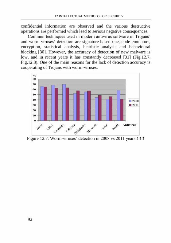
12 INTELLECTUAL METHODS FOR SECURITY

92

confidential information are observed and the various destructive

operations are performed which lead to serious negative consequences.

Common techniques used in modern antivirus software of Trojans’

and worm-viruses’ detection are signature-based one, code emulators,

encryption, statistical analysis, heuristic analysis and behavioural

blocking [30]. However, the accuracy of detection of new malware is

low, and in recent years it has constantly decreased [31] (Fig.12.7,

Fig.12.8). One of the main reasons for the lack of detection accuracy is

cooperating of Trojans with worm-viruses.

Figure 12.7: Worm-viruses’ detection in 2008 vs 2011 years!!!!!!

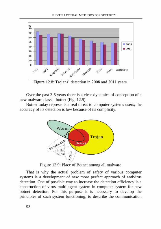
12 INTELLECTUAL METHODS FOR SECURITY

93

Figure 12.8: Trojans’ detection in 2008 and 2011 years.

Over the past 3-5 years there is a clear dynamics of conception of a

new malware class – botnet (Fig. 12.9).

Botnet today represents a real threat to computer systems users; the

accuracy of its detection is low because of its complicity.

Figure 12.9: Place of Botnet among all malware

That is why the actual problem of safety of various computer

systems is a development of new more perfect approach of antivirus

detection. One of possible way to increase the detection efficiency is a

construction of virus multi-agent system in computer system for new

botnet detection. For this purpose it is necessary to develop the

principles of such system functioning; to describe the communication

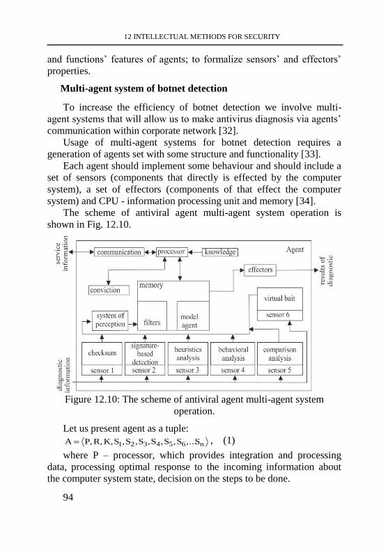
12 INTELLECTUAL METHODS FOR SECURITY

94

and functions’ features of agents; to formalize sensors’ and effectors’

properties.

Multi-agent system of botnet detection

To increase the efficiency of botnet detection we involve multi-

agent systems that will allow us to make antivirus diagnosis via agents’

communication within corporate network [32].

Usage of multi-agent systems for botnet detection requires a

generation of agents set with some structure and functionality [33].

Each agent should implement some behaviour and should include a

set of sensors (components that directly is effected by the computer

system), a set of effectors (components of that effect the computer

system) and CPU - information processing unit and memory [34].

The scheme of antiviral agent multi-agent system operation is

shown in Fig. 12.10.

Figure 12.10: The scheme of antiviral agent multi-agent system

operation.

Let us present agent as a tuple:

n654321 S,...S,S,S,S,S,S,K,R,PA , (1)

where P – processor, which provides integration and processing

data, processing optimal response to the incoming information about

the computer system state, decision on the steps to be done.

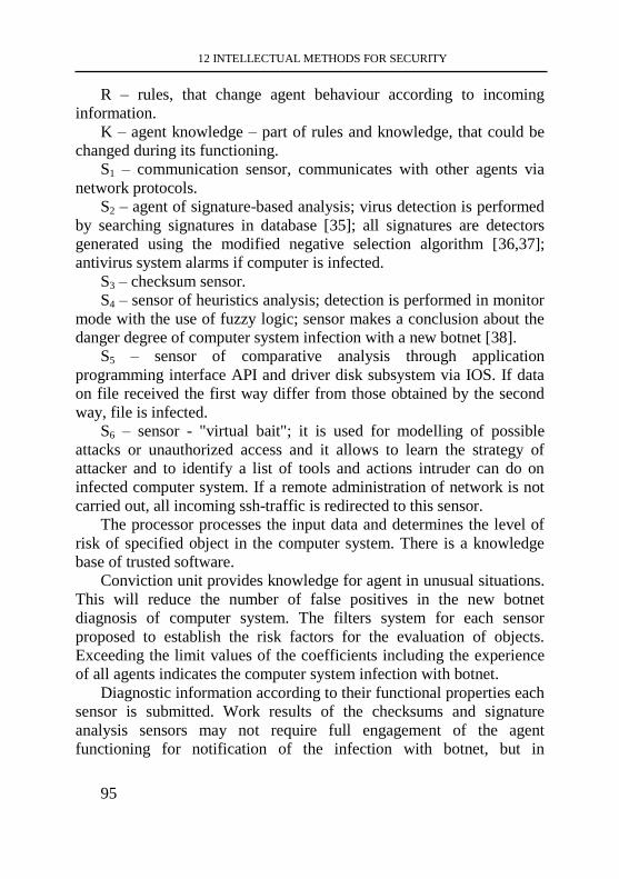
12 INTELLECTUAL METHODS FOR SECURITY

95

R – rules, that change agent behaviour according to incoming

information.

K – agent knowledge – part of rules and knowledge, that could be

changed during its functioning.

S1 – communication sensor, communicates with other agents via

network protocols.

S2 – agent of signature-based analysis; virus detection is performed

by searching signatures in database [35]; all signatures are detectors

generated using the modified negative selection algorithm [36,37];

antivirus system alarms if computer is infected.

S3 – checksum sensor.

S4 – sensor of heuristics analysis; detection is performed in monitor

mode with the use of fuzzy logic; sensor makes a conclusion about the

danger degree of computer system infection with a new botnet [38].

S5 – sensor of comparative analysis through application

programming interface API and driver disk subsystem via IOS. If data

on file received the first way differ from those obtained by the second

way, file is infected.

S6 – sensor - "virtual bait"; it is used for modelling of possible

attacks or unauthorized access and it allows to learn the strategy of

attacker and to identify a list of tools and actions intruder can do on

infected computer system. If a remote administration of network is not

carried out, all incoming ssh-traffic is redirected to this sensor.

The processor processes the input data and determines the level of

risk of specified object in the computer system. There is a knowledge

base of trusted software.

Conviction unit provides knowledge for agent in unusual situations.

This will reduce the number of false positives in the new botnet

diagnosis of computer system. The filters system for each sensor

proposed to establish the risk factors for the evaluation of objects.

Exceeding the limit values of the coefficients including the experience

of all agents indicates the computer system infection with botnet.

Diagnostic information according to their functional properties each

sensor is submitted. Work results of the checksums and signature

analysis sensors may not require full engagement of the agent

functioning for notification of the infection with botnet, but in

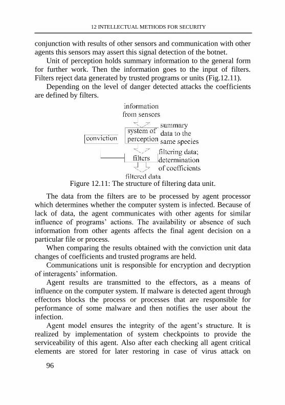
12 INTELLECTUAL METHODS FOR SECURITY

96

conjunction with results of other sensors and communication with other

agents this sensors may assert this signal detection of the botnet.

Unit of perception holds summary information to the general form

for further work. Then the information goes to the input of filters.

Filters reject data generated by trusted programs or units (Fig.12.11).

Depending on the level of danger detected attacks the coefficients

are defined by filters.

Figure 12.11: The structure of filtering data unit.

The data from the filters are to be processed by agent processor

which determines whether the computer system is infected. Because of

lack of data, the agent communicates with other agents for similar

influence of programs’ actions. The availability or absence of such

information from other agents affects the final agent decision on a

particular file or process.

When comparing the results obtained with the conviction unit data

changes of coefficients and trusted programs are held.

Communications unit is responsible for encryption and decryption

of interagents’ information.

Agent results are transmitted to the effectors, as a means of

influence on the computer system. If malware is detected agent through

effectors blocks the process or processes that are responsible for

performance of some malware and then notifies the user about the

infection.

Agent model ensures the integrity of the agent’s structure. It is

realized by implementation of system checkpoints to provide the

serviceability of this agent. Also after each checking all agent critical

elements are stored for later restoring in case of virus attack on

12 INTELLECTUAL METHODS FOR SECURITY

97

antivirus multi-agent system or possible failures in the computer

system.

Each agent can activate the recheck the selected number of sensors

to refine the results.

In situation when agent cannot communicate with other agent it is

as autonomous unit and is able to detect different malware relying on

knowledge of the latest updates and corrections in the trusted software

baseIt is advisable to keep all the given values.

Sensor of botnet detection in monitor mode

A new technique for sensor diagnosis in monitor mode which uses

fuzzy logic was developed. It is based on behavioural model of

malware [38]. This sensor enables to make a conclusion about the

degree of danger of computer system infection by malware. For this

purpose we construct the input and output linguistic variables with

names: "suspicion degree of software object" - for the input linguistic

variable, and "danger degree of the infection” - for output one.

The task of determination of membership function for input

variable we will consider as the task of the ranking for each of

mechanisms (functions) im of penetration ports jp with the set of

indications of danger Z and a choice of the most possible jp with

activation of some function im . Then we generate a matrix of

advantage ijadv qM . Elements of given matrix ijq are positive

numbers: jiij q/qq , ijq0 ; ijj i q/1q , 1qii , l,1j,i , l - amount

of possible results. Elements ijq of matrix advM are defined by

calculation of values of pair advantages to each indication separately

taking into account their scales }z{Z k ; r,1k with usage of such

formula

r

1k

kkjk

r

1k

kkijij pq/pqq . (2)

Eigenvector ),...,( m1 is defied by using a matrix of

advantage. This eigenvector answers maximum positive radical of

12 INTELLECTUAL METHODS FOR SECURITY

98

characteristic polynomial 0EMadv . S , where E is an

identity matrix.

Elements of vector П ( 1i ) are identified with an estimation of

experts who consider the accepted indications of danger. The same

procedure is performed for all im . As a result we receive a matrix of

relationship |p,m|V jip , in which each pair (relationship) im , jp

value 10 responds.

Using matrix |p,m|V jip , we build matrix |p,m|V ji*p in which

the relationship ( ji p,m ) is used and the elements of this relationship

have value max ( 10 max ). Using matrix |p,m|V ji*p , we build

normalized curve for membership function )R(pX of an input

variable.

Example of possible 20 pairs )y,x( ji ranked by the suspicion

degree is given in Fig.7. Formation of function membership and at the

stages of activation )R(aX and executing of the destructive actions

)R(eX are similar.

As a part of the solution of the problem the FIS using Mamdani

algorithm was realized (Fig. 12.12-13).

The results of fuzzy inference system 0.804 are interpreted as the

degree of computer system infection with malware. If the resulting number

exceeds some adopted threshold of danger antivirus system will block

actions of the aqueous object. The sensor also transmits information about

suspicious software to other agents.

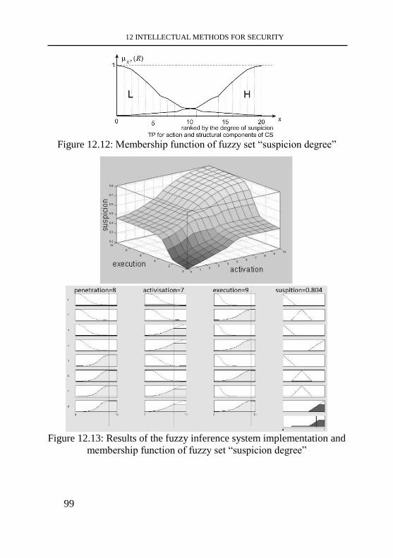
12 INTELLECTUAL METHODS FOR SECURITY

99

Figure 12.12: Membership function of fuzzy set “suspicion degree”

Figure 12.13: Results of the fuzzy inference system implementation and

membership function of fuzzy set “suspicion degree”

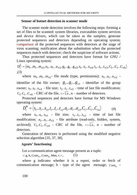
12 INTELLECTUAL METHODS FOR SECURITY

100

Sensor of botnet detection in scanner mode

The scanner mode detection involves the following steps: forming a

set of files to be scanned: system libraries, executables system services

and device drivers, which can be taken as the samples; generate

protected sequences and detectors depending on operating system;

comparison of the protected sequences with detectors at the stage of

virus scanning; notification about the substitution when the protected

sequences match with detector; check the suspicion of software actions.

Thus protected sequences and detectors have format for GNU /

Linux operating system:

6xi15xi14xi13xi12xi11xi1Li C...C...C,t...t...t,s...s...s,g...g...g,u...u...u,m...m...mD

,(3)

where 1xi1 m...m...m - file mode (type, permissions); 2xi1 u...u...u -

identifier of the file owner; 31 ...... xi ggg - identifier of the group

owner; 4xi1 s...s...s - file size; 5xi1 t...t...t - time of last file modification;

6xi1 C...C..C - CRC of the file, n,1i , n – number of detectors.

Protected sequences and detectors have format for MS Windows

operating system:

41312111 ......,......,......,...... zizizizi

W

i CCCaaatttsssD (4)

where 1zi1 s...s...s - file size; 2zi1 t...t...t - time of last file

modification; 3zi1 a...a...a - file attribute (read-only, hidden, system,

archived); 4zi1 C...C..C - CRC of the file, ni ,1 , n - number of

detectors.

Generation of detectors is performed using the modified negative

selection algorithm [35, 37, 38].

Agents’ functioning

Let a communication agent message present as a tuple:

tMes,,Com ,Com h, g, yx , (5)

where g indicates whether it is a report, order or fetch of

communication message; h - type of the agent message; yCom -

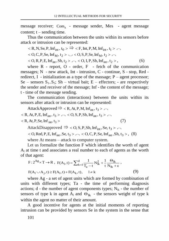
12 INTELLECTUAL METHODS FOR SECURITY

101

message receiver; xCom - message sender, Mes - agent message

content; t – sending time.

Thus the communication between the units within its sensors before

attack or intrusion can be represented:

0int t,Inf P,Se,N,R, 1int t,Inf M,P,Int, F,

2M t,Inf Se,P,C,O, 2M t,Inf Se,P,S, O,

2int tSh,,Inf E,P,R, O, 2int t,Inf Sh, P,I, O, , (6)

where R - report, O - order, F - fetch of the communication

messages; N - new attack, Int - intrusion, C - continue, S - stop, Red -

redirect, I - initialization as a type of the massage; P – agent processor;

Se – sensors S1..S5; Sh – virtual bait; E – effectors; - are respectively

the sender and receiver of the message; Inf - the content of the message;

t - time of the message sending.

The communication (interactions) between the units within its

sensors after attack or intrusion can be represented:

AttackApproved 3int t,Inf M,P,At, R,

3int t,Inf E,P,At, R, 3int t,Inf Sh,P,S, O,

3int t,Inf Se,P,At, R, (7)

AttackDisapproved 3int tSe,,Inf Sh,P,S, O,

3int tSe,,Inf E,P,Red,O, 3int tSh,,Inf Se,P,C,O, , (8)

where At means – attack to computer system.

Let us formalize the function F which identifies the worth of agent

Al at time t and associates a real number to each of agents as the worth

of that agent:

RT2:F Ag ,

lk

lkd

1k

2lk

al

Nt

1N

tT

1)t,A(F ,

kl,)t,A(F)t,A(F)t,AA(F kljl (9)

where Ag - a set of agent units which are formed by combination of

units with different types; Ta - the time of performing diagnosis

actions; d - the number of agent components types; Nlk - the number of

sensors of type k in agent Al and lk - the sensors weight of type k

within the agent no matter of their amount.

A good incentive for agents at the initial moments of reporting

intrusion can be provided by sensors Se in the system in the sense that

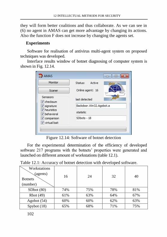
12 INTELLECTUAL METHODS FOR SECURITY

102

they will form better coalitions and thus collaborate. As we can see in

(6) no agent in AMAS can get more advantage by changing its actions.

Also the function F does not increase by changing the agents set.

Experiments

Software for realisation of antivirus multi-agent system on proposed

techniques was developed.

Interface results window of botnet diagnosing of computer system is

shown in Fig. 12.14.

Figure 12.14: Software of botnet detection

For the experimental determination of the efficiency of developed

software 217 programs with the botnets’ properties were generated and

launched on different amount of workstations (table 12.1).

Table 12.1: Accuracy of botnet detection with developed software.

Workstations

(agents)

Botnets

(number)

16 24 32 40

SDbot (80) 74% 75% 78% 81%

Rbot (49) 61% 63% 64% 67%

Agobot (54) 60% 60% 62% 63%

Spybot (18) 65% 68% 71% 75%

12 INTELLECTUAL METHODS FOR SECURITY

103

Mytob (16) 54% 57% 60% 63%

Accuracy, % 62.8% 64.6% 67.8% 69.8%

Accuracy of botnet detection of the developed software in comparison

with known is shown in Fig. 12.14, it shows growth of accuracy by 3-5%

in comparison with known antivirus software.

Also we performed false detection experiments and it is about 3-7%.

But with the growth of agents amount false detection is reducing to 2-4%.

Conclusions

This section showed an approach for the botnet detection based on

multi-agent system is proposed. A technique for sensor diagnosis in

monitor mode which uses fuzzy logic is presented. The principles of

communication between the agent’s units before and after attack on the

computer system were described. A new technique for sensor diagnosis

in scanner mode with generation of detectors using the modified

negative selection algorithm was illustrated.

12.3 Technique for bots detection which use polymorphic code

Introduction

Today the problem of cyber security is very important because the

data protection problem is extremely relevant.

Virus detection is a very important task because the information

pilfering, anonymous access to network, spy actions, spamming are

observed.

The most dangerous occurrence in the virus elaboration is botnet -

network of private computers infected with malicious software and

controlled as a group without the owners' knowledge, e.g. to send spam

[39].

Some examples of the most dangerous botnet are Virut, which have

infected over 3 million unique users computer systems according to the

report "Kaspersky Lab" [40]; botnet Zeus, is designed to attack servers

and intercept personal data (damage for European customers is about €

36 million); botnet Kelihos, which performs abduction of passwords

stored in the browser, sends spam, steals users’ credentials. All

mentioned botnets include the self-defense modules, which have

contributed to their rapid spread and inefficient detection [41,42].

12 INTELLECTUAL METHODS FOR SECURITY

104

These facts indicate a lack of effectiveness of the known detection

methods. That is why an important task is to build new techniques and

approaches to identify botnet, which will take into account its

properties and availability of hiding module.

Related works

To conceal the presence of botnet, the polymorphism technology is

used.

For polymorphic malwares, the decryptor part of the virus is

mutated at each infection, thanks to common obfuscation techniques:

“garbage-commands” insertion, register reassignment, and instruction

replacement. In order to detect such high-mutating viruses, several

solutions have been developed.

Byte-level detection solutions. Current antiviral solutions use

different techniques in order to detect malicious files. The techniques

are: pattern-matching, emulation, dynamic behavioral detection, and

various heuristics [43]. Authors focused on pattern-matching

techniques (heuristics are aimed at new malware detection and are

subject to a high false positive rates, while emulation may not always

succeed; dynamic malware detection, while achieving good results, is

out of the scope of this chapter). Because they have time and

complexity constraints, the models and detection algorithms used in

today’s antiviral products are relatively simple. The detection algorithm

consists of determining whether a given binary program is recognized

by one of the viral signature. Since regular expressions are used as

signature descriptions, antivirus products may use finite state

automatons to perform linear-time detection.

Another emerging approach consists of using machinelearning

techniques in order to detect malicious files [44]. Several models have

been tested: data-mining [45], Markov chains on n-grams [46,47],

Naive Bayes as well as decision trees [48]. These methods provide an

automatic way to extract signature from malicious executables. But

while the experiments have shown good results, the false positive and

negative rates are still not negligible.

Structural and semantic models. In [49,50], graphs are used as a

model for malwares. The control flow graph (CFG) of a malware is

computed (when possible) and reduced. Then, subsets of this graph are

12 INTELLECTUAL METHODS FOR SECURITY

105

used as a signature. Detection of a malware is done by comparing a

suspicious file against these sub-CFGs, and seeing if any part of the

CFG of the file is equivalent (with a semantics-aware equivalence

relation for [51]) to a sub-CFG in the viral database. The idea is that

most of mutation engines’ obfuscations do not alter the control flow

graph of the malware.

CTPL is a variant of CTL [52], able to handle register-renaming

obfuscation. Detection is done via model checking of API call

sequence, while signatures extraction is done manually.

A promising approach was initiated by Preda et. al [53]. It consists

in using the semantics of a metamorphic malware as a viral signature.

None of them provides an automated process to extract this grammar

for a given malware.

Background

In [54] botnet detection technique for determining the degree of

presence of botnet based on multi-agent systems was proposed. Offered

method was based on analyzing the bots actions demonstration in

corporate area network. Technique provides propose the construction of

a schematic map of connections which is formed by corresponding

records in each antiviral agent of multi-agent systems for some

corporate area network. All agents based on this information can

perform communicative exchange data to each other. Proposed method

is based on analyzing the bots actions demonstration in situations of

intentional change of connection type in probably infected computer

system.

During computer system (CS) is functioning the antivirus detection

via sensors available in an each agent is performed. The antivirus

diagnosis results are analyzed in order to define which of sensors have

triggered and what suspicion degree it has produced. If triggering

sensors are signature 1S or checksum 2S analyzers, the results 1SR and

2SR are interpreted as a 100% malware detection. In this situation, the

blocking of software implementation and its subsequent removal are

performed.

For situations when the sensors of heuristic 3S and behavioral 4S

analyzers have triggered, the suspicion degrees 3SR and 4SR are

12 INTELLECTUAL METHODS FOR SECURITY

106

analyzed, and in the case of overcoming of the defined certain threshold

n, 100),max( 43 SS RRn , the blocking of software implementation and

its subsequent removal are performed. If the specified threshold hasn’t

overcome the results 3SR , 4SR are analyzed whether they belong to

range nRRm SS ),max( 43 in order to make the final decision about

malware presence in CS. If the value is mRR SS ),max( 43 than the new

antivirus results from sensors are expected. In all cases the antiviral

agents information of infection or suspicion software behavior in

computer system is must be sent out to other agents.

The important point of this approach is to research the situation

where the results of antivirus diagnosis belong to range

nRRm SS ),max( 43 . In this case, the antiviral agent of CS asks other

agents in the corporate area network about the similarity of suspicion

behavior of some software that is similar to the botnet. After that the

analysis of botnet demonstrations on computer systems of the corporate

area network and the definition of the degree of a new botnet presence

in the network was determined. The presence of botnet in the corporate

area network was concluded by the fuzzy expert system that confirmed

or disproved this fact.

The developed system has been demonstrating the efficiency of

botnet detection at about 88-96%.

As some botnets use the technology of hiding malicious code

(polymorphic code) today, mentioned multi-agent systems for botnet

detection, where bots used such technology, have been tested. Test

results were unexpected. It turned out that the developed system was

not fully adapted to detect polymorphic code, and efficiency decreased

by 7-12%. Also after retest some bots were detected, which had been

previously identified and removed (all bots contained the polymorphic

code).

That is why the actual problem is a development of a new botnet

detection technique that will find out the polymorphic code in bots.

Technique for bots detection which use polymorphic code

In order to develop the technique we have to investigate the

properties of polymorphic viruses. They create varied (though fully

functional) copies of themselves as a way to avoid detection by anti-

12 INTELLECTUAL METHODS FOR SECURITY

107

virus software. Some polymorphic virus use different encryption

schemes and require different decryption routines. Thus, the same virus

may look completely different on different systems or even within

different files. Other polymorphic viruses vary instruction sequences

and use false commands in the attempt to thwart anti-virus software.

One of the most advanced polymorphic viruses uses a mutation engine

and random-number generators to change the virus code and its

decryption routine [55].

Levels of polymorphism

Today 6 polymorphism levels are known [56]. Let us build models

for all the levels of polymorphism.

The first level of polymorphism

Viruses of the first polymorphism level use the constant set of

actions for different decryption modules. They can be detected by some

areas of permanent code decryption.

Let us present the virus model for the first level of polymorphism as

a tuple

)R,P,Q,,U,G,X,V,A(M1 ,

where naaA ,...,1 - a set of commands of some program which can

be infected with virus; V – a set of virus commands for selection of one

of the present decryption modules in virus, mV ,...,1 ; X - a set of

decryption modules which are present in virus, y1 x,...,xX ; G - set of

virus commands of the xi decryption module, }g,..,g{Gxixi1

; U - a

set of malicious commands (virus body), wuuU ,...,1 ; - a function

for selection of decryption module xi, ,XV: Xxi ; Q – a

function of creation the malicious commands (virus body) by the means

of commands Ggix of the decryption’s module xi, UG:Q

ix ; P –

a function of creation the polymorphic virus behavior R by the means

of inserting the malicious commands U into program’s commands A,

RUAP : ; function of creation the polymorphic virus behavior R

without inserting malicious commands U into program’s commands A

12 INTELLECTUAL METHODS FOR SECURITY

108

only by the means of the decryption virus body U appears as

RU:Q .

Thus, polymorphic virus has its behavior that is formed by some

sequences of commands. Based on this we can build the virus behavior

as sequences.

Virus behavior A1R of the first polymorphism level which is

created by the means of inserting the malicious commands U into

program’s commands A and virus behavior 1R which is created

without inserting the malicious commands U into program’s commands

A can be presented as sequences:

w1n1xx

A1 u...ua...ag...gR

, w1xx1 u...ug...gR

where values

, indicate that possible virus commands of decryption module

xx

g...g can vary for different decryption modules x , - number

of the selected decryption module.

The second level of polymorphism

The second level of polymorphism includes viruses, which

decryption module has constant one or more instructions. For example,

they may use different registers or instructions in some alternative

decryption module. These viruses can also be identified by a specific

signature in the decryption module [56].

Let us present the virus model for the second level of

polymorphism as a tuple

),,,,,(2 RZPUEAM

where A - a set of commands of some program which can be

infected with virus, }a,...,a{A n1 ; E – a set of virus commands of the

decryption module, )...1( eeE ; U - a set of malicious commands

(virus body), wuuU ,...,1 ; Z – a function of creation the malicious

commands (virus body) by the means of selection of the present

decryption module’s commands, UE:Z ; Р -

a function of creation

the polymorphic virus behavior R by the means of inserting malicious

commands U into program’s commands A, RUAP : ; function of

12 INTELLECTUAL METHODS FOR SECURITY

109

creation the polymorphic virus behavior R without inserting malicious

commands U into program’s commands A appears as: RUE:Z .

Virus behaviors A2R and 2R of the second polymorphism level can

be presented as sequences:

w1n1A2 u...ua...ag...eR , w12 u...ug...eR , where values ,

indicate that possible virus commands g...e of decryption module can

vary for each new start of virus.

The third/fourth levels of polymorphism

Viruses that use decryption commands and do not decrypt the virus

code and have a “garbage-commands” refer to the third level of

polymorphism. These viruses can be determined using a signature if all

the “garbage-commands” are discarded. Viruses of the fourth level use

the interchangeable or "mixed" instructions for the decryption without

changing the decryption algorithm.

Let us present the virus model for the third and fourth levels of

polymorphism as a tuple ),,,,,,(4,3 RDYBUEAM

where A - a set of commands of some program which can be

infected with virus, }a,...,a{A n1 ; E – a set of virus commands of the

decryption module, )...1( eeE ; U - a set of malicious commands

(virus body), }u,...,u{U w1 ; B – a set of the “garbage-commands”,

tbbB ,...,1 ; Y – a function of creation the malicious commands (virus

body) by the means of decryption module, that integrates the “garbage-

commands” into malicious commands, UBE:Y ; D - a function of

creation the polymorphic virus behavior R by the means of virus body

inserting malicious commands U into program’s commands A,

RUA:D ; function of creation the polymorphic virus behavior R

without inserting malicious commands U into program’s commands A

appears as: RBE:Y .

Virus behaviors A3R ,

A4R of the third and fourth polymorphism

levels which are created by the means of decryption module, that

integrates the “garbage-commands” into malicious commands and

12 INTELLECTUAL METHODS FOR SECURITY

110

inserts malicious commands U into program’s commands A and virus

behaviors 3R , 4R without inserting malicious commands U into

program’s commands A can be presented as sequences:

bu...bua...ae...eR w1n11A3 , bu...bue...eR w113 ,

bu...bua...ae...eR n11A4 , bu...bue...eR 14 , where values , ,

, indicate that possible “garbage-commands” and virus commands

bu...bu can vary for each new start of virus.

The fifth level of polymorphism

The fifth level of polymorphism includes all properties of the above

levels, and the decryption module may use different algorithms for

decrypting the virus code.

Let us present the virus model for the fifth level of polymorphism

as a tuple

)R,D,H,,U,G,X,B,V,A(M5

where A - a set of commands of some program which can be

infected with virus, }a,...,a{A n1 ; V – a set of commands for selection

of one of the present decryption modules in virus, },...,{V m1 ; X - a

set of decryption modules which are present in virus, y1 x,...,xX ; G -

a set of virus commands of the decryption module xi, }g,..,g{Gxixi1

;

U - a set of malicious commands (virus body), wuuU ,...,1 ; - a

function for selection of decryption module xi, ,XV: ,Xxi ; B -

a set of the “garbage-commands”, hbbB ,...,1 ; Н - a function of

creation the malicious commands (virus body) by the means of

selection of the present decryption module’s xi commands Ggix and

generation the order of its execution, UGB:Hix ; D - a function of

creation the polymorphic virus behavior R by the means of inserting

malicious commands U program’s commands A, RUAD : ;

function of creation the polymorphic virus behavior R without inserting

malicious commands U into program’s commands A by the means of

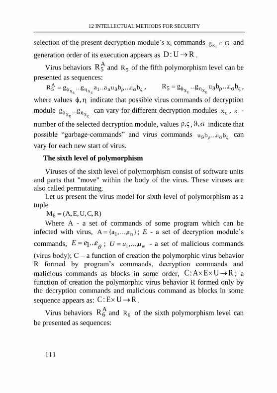
12 INTELLECTUAL METHODS FOR SECURITY

111

selection of the present decryption module’s xi commands Ggix and

generation order of its execution appears as RU:D .

Virus behaviors A5R and 5R of the fifth polymorphism level can be

presented as sequences:

bu...bua...ag...gR n1xx

A5 ,

bu...bug...gR

xx5 ,

where values , indicate that possible virus commands of decryption

module

xxg...g can vary for different decryption modules x , -

number of the selected decryption module, values , , , indicate that

possible “garbage-commands” and virus commands bu...bu can

vary for each new start of virus.

The sixth level of polymorphism

Viruses of the sixth level of polymorphism consist of software units

and parts that "move" within the body of the virus. These viruses are

also called permutating.

Let us present the virus model for sixth level of polymorphism as a

tuple

)R,C,U,E,A(M6

Where A - a set of commands of some program which can be

infected with virus, }a,...,a{A n1 ; E - a set of decryption module’s

commands,

eeE ...1 ; wuuU ,...,1 - a set of malicious commands

(virus body); С – a function of creation the polymorphic virus behavior

R formed by program’s commands, decryption commands and

malicious commands as blocks in some order, RUEA:C ; a

function of creation the polymorphic virus behavior R formed only by

the decryption commands and malicious command as blocks in some

sequence appears as: RUE:C .

Virus behaviors A6R and 6R of the sixth polymorphism level can

be presented as sequences:

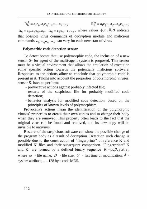
12 INTELLECTUAL METHODS FOR SECURITY

112

ua..uaea..eaR n1ii1A6 , uea...aueaR n21

A6 ,

u..ue..eR6 , ue...ueR6 , where values , , , indicate

that possible virus commands of decryption module and malicious

commands u..ue..e can vary for each new start of virus.

Polymorhic code detection sensor

To detect botnet that use polymorphic code, the inclusion of a new

sensor S7 for agent of the multi-agent system is proposed. This sensor

must be a virtual environment that allows the emulation of execution

some specific action towards the potentially malicious software.

Responses to the actions allow to conclude that polymorphic code is

present in it. Taking into account the properties of polymorphic viruses,

sensor S7 have to perform:

- provocative actions against probably infected file;

- restarts of the suspicious file for probably modified code

detection;

- behavior analysis for modified code detection, based on the

principles of known levels of polymorphism.

Provocative actions mean the identification of the polymorphic

viruses’ properties to create their own copies and to change their body

when they are removed. This property often leads to the fact that the

original virus can be found and removed, and its new copy will be

invisible to antivirus.

Restarts of the suspicious software can show the possible change of

the program body as a result of decryption. Detection such change is

possible due to the construction of "fingerprints" of reference K and

modified K' files and their subsequent comparison. "Fingerprints" K

and K’ are formed by a defined binary sequence ,,,,K ,

where - file name; - file size; - last time of modification; -

system attribute; - 128 byte code MD5.

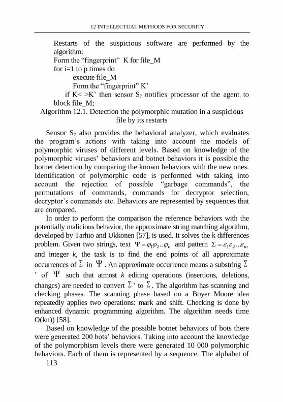
12 INTELLECTUAL METHODS FOR SECURITY

113

Restarts of the suspicious software are performed by the

algorithm:

Form the “fingerprint” K for file_M

for i=1 to p times do

execute file_M

Form the “fingerprint” K’

if K< >K’ then sensor S7 notifies processor of the agenti to

block file_M;

Algorithm 12.1. Detection the polymorphic mutation in a suspicious

file by its restarts

Sensor S7 also provides the behavioral analyzer, which evaluates

the program’s actions with taking into account the models of

polymorphic viruses of different levels. Based on knowledge of the

polymorphic viruses’ behaviors and botnet behaviors it is possible the

botnet detection by comparing the known behaviors with the new ones.

Identification of polymorphic code is performed with taking into

account the rejection of possible “garbage commands”, the

permutations of commands, commands for decryptor selection,

decryptor’s commands etc. Behaviors are represented by sequences that

are compared.

In order to perform the comparison the reference behaviors with the

potentially malicious behavior, the approximate string matching algorithm,

developed by Tarhio and Ukkonen [57], is used. It solves the k differences

problem. Given two strings, text n ...21 and pattern m ...21

and integer k, the task is to find the end points of all approximate

occurrences of in . An approximate occurrence means a substring

’ of such that atmost k editing operations (insertions, deletions,

changes) are needed to convert ’ to . The algorithm has scanning and

checking phases. The scanning phase based on a Boyer Moore idea

repeatedly applies two operations: mark and shift. Checking is done by

enhanced dynamic programming algorithm. The algorithm needs time

O(kn)) [58].

Based on knowledge of the possible botnet behaviors of bots there

were generated 200 bots’ behaviors. Taking into account the knowledge

of the polymorphism levels there were generated 10 000 polymorphic

behaviors. Each of them is represented by a sequence. The alphabet of

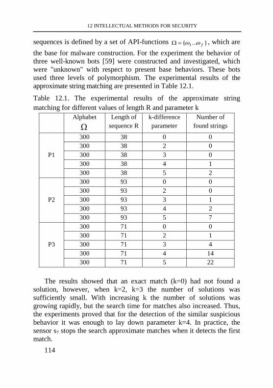
12 INTELLECTUAL METHODS FOR SECURITY

114

sequences is defined by a set of API-functions }...{ 1 f , which are

the base for malware construction. For the experiment the behavior of

three well-known bots [59] were constructed and investigated, which

were "unknown" with respect to present base behaviors. These bots

used three levels of polymorphism. The experimental results of the

approximate string matching are presented in Table 12.1.

Table 12.1. The experimental results of the approximate string

matching for different values of length R and parameter k

Alphabet

Length of

sequence R

k-difference

parameter

Number of

found strings

P1

300 38 0 0

300 38 2 0

300 38 3 0

300 38 4 1

300 38 5 2

P2

300 93 0 0

300 93 2 0

300 93 3 1

300 93 4 2

300 93 5 7

P3

300 71 0 0

300 71 2 1

300 71 3 4

300 71 4 14

300 71 5 22

The results showed that an exact match (k=0) had not found a

solution, however, when k=2, k=3 the number of solutions was

sufficiently small. With increasing k the number of solutions was

growing rapidly, but the search time for matches also increased. Thus,

the experiments proved that for the detection of the similar suspicious

behavior it was enough to lay down parameter k=4. In practice, the

sensor s7 stops the search approximate matches when it detects the first

match.

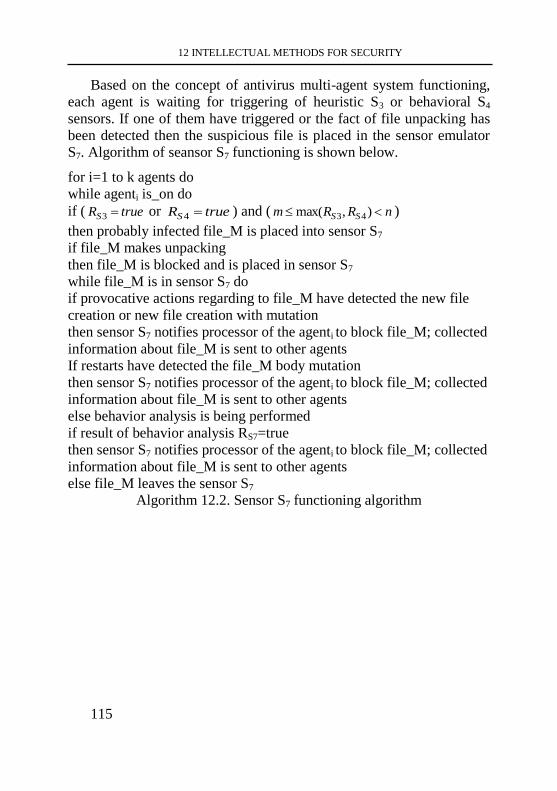
12 INTELLECTUAL METHODS FOR SECURITY

115

Based on the concept of antivirus multi-agent system functioning,

each agent is waiting for triggering of heuristic S3 or behavioral S4

sensors. If one of them have triggered or the fact of file unpacking has

been detected then the suspicious file is placed in the sensor emulator

S7. Algorithm of seansor S7 functioning is shown below.

for i=1 to k agents do

while agenti is_on do

if ( trueRS 3 or trueRS 4 ) and ( nRRm SS ),max( 43 )

then probably infected file_M is placed into sensor S7

if file_M makes unpacking

then file_M is blocked and is placed in sensor S7

while file_M is in sensor S7 do

if provocative actions regarding to file_M have detected the new file

creation or new file creation with mutation

then sensor S7 notifies processor of the agenti to block file_M; collected

information about file_M is sent to other agents

If restarts have detected the file_M body mutation

then sensor S7 notifies processor of the agenti to block file_M; collected

information about file_M is sent to other agents

else behavior analysis is being performed

if result of behavior analysis RS7=true

then sensor S7 notifies processor of the agenti to block file_M; collected

information about file_M is sent to other agents

else file_M leaves the sensor S7

Algorithm 12.2. Sensor S7 functioning algorithm

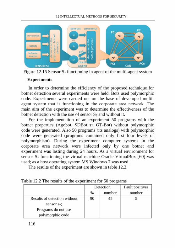
12 INTELLECTUAL METHODS FOR SECURITY

116

Figure 12.15 Sensor S7 functioning in agent of the multi-agent system

Experiments

In order to determine the efficiency of the proposed technique for

botnet detection several experiments were held. Bots used polymorphic

code. Experiments were carried out on the base of developed multi-

agent system that is functioning in the corporate area network. The

main aim of the experiment was to determine the effectiveness of the

botnet detection with the use of sensor S7 and without it.

For the implementation of an experiment 50 programs with the

botnet properties (Agobot, SDBot та GT-Bot) without polymorphic

code were generated. Also 50 programs (its analogs) with polymorphic

code were generated (programs contained only first four levels of

polymorphism). During the experiment computer systems in the

corporate area network were infected only by one botnet and

experiment was lasting during 24 hours. As a virtual environment for

sensor S7 functioning the virtual machine Oracle VirtualBox [60] was

used; as a host operating system MS Windows 7 was used.

The results of the experiment are shown in table 12.2.

Table 12.2 The results of the experiment for 50 programs

Detection Fault positives

% number number

Results of detection without

sensor s7;

Programs do not use

polymorphic code

90 45 5

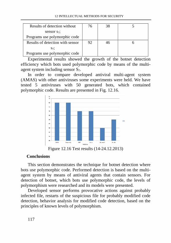
12 INTELLECTUAL METHODS FOR SECURITY

117

Results of detection without

sensor s7;

Programs use polymorphic code

76 38 5

Results of detection with sensor

s7;

Programs use polymorphic code

92 46 6

Experimental results showed the growth of the botnet detection

efficiency which bots used polymorphic code by means of the multi-

agent system including sensor S7.

In order to compare developed antiviral multi-agent system

(AMAS) with other antiviruses some experiments were held. We have

tested 5 antiviruses with 50 generated bots, which contained

polymorphic code. Results are presented in Fig. 12.16.

Figure 12.16 Test results (14-24.12.2013)

Conclusions

This section demonstrates the technique for botnet detection where

bots use polymorphic code. Performed detection is based on the multi-

agent system by means of antiviral agents that contain sensors. For

detection of botnet, which bots use polymorphic code, the levels of

polymorphism were researched and its models were presented.

Developed sensor performs provocative actions against probably

infected file, restarts of the suspicious file for probably modified code

detection, behavior analysis for modified code detection, based on the

principles of known levels of polymorphism.

12 INTELLECTUAL METHODS FOR SECURITY

118

Results of the experiments have demonstrated the increase of the

botnet detection efficiency by 16% with involving the sensor S7

compared to its absence. Thus the growth of false positives is not

significant.

The disadvantage of the proposed technique is sufficiently large

computational complexity of the behavior analysis that is based on the

principles of polymorphism levels.

Advancement questions

11. What kind of process is called Intrusion Detection System

(IDS) and what is its purpose?

12. What are the three major components and categories of an IDS?

13. Name general characteristics of the basic categories of IDS.

14. What is the difference between AI (Artificial Intelligence) and

CI (Computer Intelligence)?

15. What are the three common algorithms of the Machine

Learning concept?

16. What is the Artificial Neural Networks technique and how they

could be applied in IDS?

17. What are the main dificaties of the polymorphic code detectin?

18. Name all existing levels of polymorphism and how they can be

detected?

19. Explain the idea of polymorphic code detection using sensor

approach.

20. What is the virtual the emulation of execution some specific

action towards the potentially malicious software for?

REFERENCE

1. Fatai Adesina Anifowose Safiriyu Ibiyemi Eludiora Application

of Artificial Intelligence in Network Intrusion Detection / Fatai

12 INTELLECTUAL METHODS FOR SECURITY

119

Adesina Anifowose Safiriyu Ibiyemi Eludiora // World Applied

Programming.- 2012. - Vol (2), No (3). – pp. 158-166.

2. Lee C.H. International Conference on Fuzzy Systems / C.H.

Lee, Y. C. Lin // Hybrid Learning Algorithm for Neuro-Fuzzy

Systems”, Proceedings. 2004 IEEE - 2004. -p691-696.

3. Artail H. A Hybrid Honeypot Framework for Improving

Intrusion Detection Systems Organizational Networks / H.

Artail, H. Safa, M. Sraj, I. Kuwatly, Z. Al-Masri // Journal of

Computers & Security.- 2006. - Vol. 25 -p274 – 288.

4. Eduardo J., and Brandão M.S. A New Approach for IDS

Composition / J. Eduardo, M.S. Brandão // IEEE International

Conference on Communications. - 2006.-p2195-2200.

5. Watkins A. An Immunological Approach to Intrusion Detection

/ A. Watkins // 12th Annual Canadian Information Technology

Security Symposium. , 2000.-p447-454.

6. Intrusion Detection System[Electronic resource]: Wikipedia,

The Free Encyclopedia, “Intrusion Detection System”, Access

mode : http://en.wikipedia.org/wiki/Intrusion-detection_system.

7. Jun H. Computational Intelligence [Electronic resource] / H.

Jun // Research Interests - Access mode :

http://www.cs.bham.ac.uk/~jxh/hejunrs.html.

8. Symeonidis, A. L. Agent Intelligence through Data Mining / A.

L. Symeonidis // Multi-agent Systems, Artificial Societies, and

Simulated Organizations Series 14. - 2000.-p. 200.

9. Petrus J.B. Artificial Neural Networks: An Introduction to

ANN Theory and Practice / J.B Petrus // Springer. - 1995.-p37-

57.

10. Wang Y. Fuzzy Clustering Analysis by using Genetic

Algorithm // Y. Wang //, Innovative Computing, Information

and Control Express Letters 2(4). - 2008.-p.331-337.

11. Castillo O. Intelligent Systems with Interval Type-2 Fuzzy

Logic /O. Castillo, P. Melin // International Journal of

12 INTELLECTUAL METHODS FOR SECURITY

120

Innovative Computing, Information and Control 4 (4). - 2008.-

p.771-784.

12. Mendel J. Type-2 Fuzzy Sets: Some Questions and Answers / J.

Mendel. // IEEE Connections, Newsletter of the IEEE Neural

Networks Society 1. - 2003.-p.10-13.

13. Sampada C. Adaptive Neuro-Fuzzy Intrusion Detection

Systems / C. Sampada, S. Khusbu, D. Neha, M. Sanghamitra,

A. Abraham, S. Sugata // International Conference on

Information Technology: Coding and Computing (ITCC’04),

DOI: 0-7695-2108-8/04, 2004.

14. Bashah N. Hybrid Intelligent Intrusion Detection System / N.

Bashah, I.B. Shanmugam, A.M. Ahmed // World Academy of

Science, Engineering and Technology. - 2005.-p.23-26.

15. Burges C.J. A Tutorial on Support Vector Machines for Pattern

Recognition / C.J. Burges. // Data Mining and Knowledge

Discovery 2. - 1998 -pp121-167.

16. Cristianini N. An Introduction to Support Vector Machines and

other Kernel-Based Learning Methods, 1st Edition / N.

Cristianini, and J. Shawe-Taylor. - Cambridge University Press,

UK, 2000.

17. Abe S. “Fuzzy LP-SVMs for Multiclass Problems” / S. Abe //

In Proceedings: European Symposium on Artificial Neural

Networks, Belgium -2004. - p429-434.

18. Taboada J. “Creating a Quality Map of a Slate Deposit using

Support Vector Machines” / J. Taboada, J.M. Matías, C.

Ordóñez, and P.J. García // Elsevier Journal of Computational

and Applied Mathematics 20 (4). -2007. -p84-94.

19. Xing Y. “Multiclass Least Squares Auto-Correlation Wavelet

Support Vector Machines” / Y. Xing, X. Wu, and Z. Xu //

International Journal of Innovative Computing, Information and

Control Express Letters 2 (4). -2008. -p345-350.

12 INTELLECTUAL METHODS FOR SECURITY

121

20. Zhang Z. "Application of Online Training SVMs for Real-time

Intrusion Detection with Different Considerations" // Z. Zhang,

and H. Shen // Elsevier Journal of Computer Communications,

Volume 28. -2005. -p1428-1442.

21. Mohsen S. Design of Neural Networks using Genetic

Algorithm for the Permeability Estimation of the Reservoir / S.

Mohsen, A. Morteza, and Y.V. Ali // Journal of Petroleum

Science and Engineering, Vol. 59. -2007. – p. 97–105.

22. Bies R.R. "A Genetic Algorithm-Based Hybrid Machine

Learning Approach to Model Selection" / R.R. Bies, M.F.

Muldoon, B.G. Pollock, S. Manuck, G. Smith, M.E. Sale //

Journal of Pharmacokinetics and Pharmacodynamics, Vol. 33. -

2006. P. 195-221.

23. Castillo E. "Functional Networks" / E. Castillo // Neural

Processing Letters. -1998 -Vol7. -p151–159.

24. El-Sebakhy E.A., "Software reliability identification using

functional networks: A comparative study" / E. A. El-Sebakhy

// Expert Systems with Applications, Volume 36. -2009. – p.

413-420.

25. Anifowose F. “Hybrid AI Models for the Characterization of

Oil and Gas Reservoirs: Concept, Design and Implementation”

/ F.Anifowose. -VDM Verlag, 2009.

26. Inoue H. “Efficient Pruning Method for Ensemble Self-

Generating Neural Networks” / H. Inoue, and H. Narihisa //

Journal of Systemic,Cybernetics and Informatics. -2003. -p423-

428.

27. Helmy T. “Hybrid Computational Models for the

Characterization of Oil and Gas Reservoirs” / T. Helmy, F.

Anifowose and K. Faisal // Elsevier International Journal of

Expert Systems with Applications, vol. 37. -2010. -p5353-5363.

28. Anifowose F. “Fuzzy Logic-Driven and SVM-Driven Hybrid

Computational Intelligence Models Applied to Oil and Gas

12 INTELLECTUAL METHODS FOR SECURITY

122

Reservoir Characterization” / F. Anifowose and A.

Abdulraheem // Journal of Natural Gas Science and

Engineering, Volume 3. -2011. -p505-517.

29. Goshko, S. Encyclopedia of protection against viruses / S.

Goshko. - SOLON-Pres, 2005.

30. Savenko O. Research of the antivitus technologies for malware

detection / О. Savenko, S. Lysenko, A Kryshchuk //

Proceedings of the XІІ conference "Modern informations &

electronic technologies - 2011", Vol1 – Ukraine, Odessaа,

2011. – p.95-96.

31. AV Comparatives laboratories [electronic resource] – Access

mode http://www.av-comparatives.org. – Home page name.

32. Wooldridge M. An Introduction To Multiagent Systems / M.

Wooldridge. - John Wiley & Sons LTD. - 2002. - 365 p.

33. Shoham Y. Multiagent Systems Algorithmic, Game-Theoretic,

and Logical Foundations / Y. Shoham, K. Leyton-Brown //

Cambridge University Press. - 2009. - 552 p.

34. Alkhateeb F. Multi-Agent Systems – Modeling, Control,

Programming, Simulations and Applications / F. Alkhateeb, E.

Maghayreh, I. Doush, // InTech.. - 2011. - 532 p.

35. Савенко О. Розробка процесу виявлення троянських

програм на основі використання штучних імунних систем /

Олег Савенко, Сергій Лисенко //Вісник Хмельницького

національного університету. – 2008. – №5, – С.183-188.

36. Forrest A. Serf-nonself discrimination in a computer / A.

Forrest, , L. Perelson, , R. Cherukuri // Proceedings of the IEEE

Symposium on Research in Security and Privacy. - 1996. - 13p.

37. Castro L. Artificial Immune Systems: A New Computational

Approach / L. Castro , T. Timmis. - London. :Springer-Verlag,

2001.

38. Bernikov A.R. Malware search in the distributed simulators

using the technology of fuzzy logic / A.R. Bernikov, R.P.

12 INTELLECTUAL METHODS FOR SECURITY

123

Grafov, S.M. Lysenko, O.S. Savenko // Information

technologies. - Moscow : 2011, № 10. - P.42-47.

39. Oxford Dictionaries http://www.oxforddictionaries.com/

definition/english/botnet?q=botnet.

40. Nikitina T. У Virut отобрали ключевые домены (2013),

http://www.securelist.com/ru/blog/ 207764413/

U_Virut_otobrali_ klyuchevye_domeny#page_top (in Russian).

41. Yaneza J.: ZeuS/ZBOT Malware Shapes Up in 2013 (2013),

http://blog.trendmicro.com/trendlabs-security-

intelligence/zeuszbot-malware-shapes-up-in-2013.

42. Michael E. Scott: Boston Marathon/West, Texas Spam

Campaigns (2013), http://mrpdchief.blogspot.com/2013/

04/boston-marathonwest-texas-spam-campaigns.html.

43. Szor P.: The Art of Computer Virus Research and Defense.

Addison-Wesley Professional (2005).

44. Kolter J. Z. Learning to detect malicious executables in the

wild. / J.Z. Kolter, M.A. Maloof // In: Proceedings of the tenth

ACM SIGKDD international conference on Knowledge

discovery and data mining, ser. KDD ’04. -2004. –p. 470–478.

45. Ye Y. Imds: intelligent malware detection system. / Y. Ye, D.

Wang, T. Li, D.Ye // Proceedings of the 13th ACM SIGKDD

international conference on Knowledge discovery and data

mining, ser. KDD ’07. -2007. –p. 1043–1047.

46. Griffin K. Automatic generation of string signatures for

malware detection. / K. Griffin, S. Schneider, X. Hu, T.Chiueh

// Lecture Notes in Computer Science, Springer Berlin. - vol.

5758. -2009. –p. 101–120.

47. Yan W. Toward automatic discovery of malware signature for

anti-virus cloud computing / W. Yan, E. Wu // Lecture Notes of

the Institute for Computer Sciences, Social Informatics and

Telecommunications Engineering. -2009. - vol. 4. -p724–728.

12 INTELLECTUAL METHODS FOR SECURITY

124

48. Wang J.-H. Virus detection using data mining techinques. / J.-

H. Wang , P. Deng, Y.-S. Jaw, Y.-C. Liu. // Proceedings of the

IEEE 37th Annual 2003 International Carnahan Conference on

Security Technology. -2003.

49. Christodorescu M. Static analysis of executables to detect

malicious patterns. / M. Christodorescu, S. Jha // In:

Proceedings of the 12th USENIX Security Symposium. -2003.

– p. 169–186.

50. Bonfante G. Control flow graphs as malware signatures /G.

Bonfante, M. Kaczmarek, J.-Y. Marion // International

Workshop on the Theory of Computer Viruses TCV’07, Eric

Filiol, Jean-Yves Marion, and Guillaume Bonfante, Eds.,

Nancy France. -2007.

51. Clarke E. Design and synthesis of synchronization skeletons

using branching time temporal logic. / E. Clarke, E. Emerson //

Logics of Programs, ser. Lecture Notes in Computer Science,

D. Kozen, Ed. Springer Berlin. -1982. - vol. 131. – p. 52–71.

52. Leder F.Classification and detection of metamorphic malware

using value set analysis. / F. Leder, B. Steinbock, P. Martini //

Malicious and Unwanted Software (MALWARE), 2009 4th

International. - 2009. – p. 39 – 46.

53. Preda M. A semanticsbased approach to malware detection. /

M.Preda, D. Christodorescu, M. Jha, S, Debray // ACM Trans.

Program. Lang. Syst., -2008. - vol. 30, no. 5. – p. 1–54.

54. Pomorova O. Multi-agent Based Approach for Botnet Detection

in a Corporate Area Network Using Fuzzy Logic. / O.

Pomorova, O. Savenko , S. Lysenko, A. Kryshchuk //

Kwiecien A., Gaj, P., Stera, P. (eds.) CN2013. CCIS, ,

Springer, Heidelberg Dordrecht London New York. -2013. -

vol. 370. - p.146-156.

55. Glossary. ttp://home.mcafee.com/virusinfo/glossary?ctst=1#P

(2016).

12 INTELLECTUAL METHODS FOR SECURITY

125

56. Kaspersky E. Computer viruses / Kaspersky E. – Moscow : SK-

Press, 1998.

57. Jokinen, P., Tarhio, J., Ukkonen, E.: A Comparison of

Approximate String Matching Algorithms. Software: Practice

and Experience 26(12), 1439-1458.

http://onlinelibrary.wiley.com/doi/10.1002/(SICI)1097-

024X(199612)26:12<1439::AID-SPE71>3.0.CO;2-1/abstract

(1996)

58. Smyth, B.: Computing Patterns In Strings, p. 496. Williams,

Moscow (2006)

59. http://security.ludost.net/exploits/index.php?dir=bots.

60. https://www.virtualbox.org

13 METHODS AND TECHNIQUES FOR FORMAL DEVELOPMENT AND

QUANTITATIVE ASSESSMENT. RESILIENT SYSTEMS

126

CHAPTER 13. METHODS AND TECHNIQUES FOR

FORMAL DEVELOPMENT AND QUANTITATIVE

ASSESSMENT. RESILIENT SYSTEMS

Content of the chapter 13

CHAPTER 13. Methods and Techniques for Formal Development and

Quantitative Assessment. Resilient systemsОшибка! Закладка не

определена.

Background: Concepts ............ Ошибка! Закладка не определена.

Resilience Concept ................. Ошибка! Закладка не определена.

Dependability: Basic DefinitionsОшибка! Закладка не определена.

Goal-Based Development ....... Ошибка! Закладка не определена.

System Autonomy and ReconfigurationОшибка! Закладка не определена.

Methods and Techniques for Formal Development and Quantitative

Assessment ............................. Ошибка! Закладка не определена.

Development Methodologies .. Ошибка! Закладка не определена.

Event-B Method ..................... Ошибка! Закладка не определена.

Quantitative Assessment......... Ошибка! Закладка не определена.

PRISM model checker ............ Ошибка! Закладка не определена.

Discrete-event simulation ....... Ошибка! Закладка не определена.

13 METHODS AND TECHNIQUES FOR FORMAL DEVELOPMENT AND

QUANTITATIVE ASSESSMENT. RESILIENT SYSTEMS

127

Background: Concepts

In this chapter, we give an overview of the main phenomena

concepts and properties appearing in the development of resilient

distributed systems. We consider the notion of “resilience” as an

evolution of the dependability concept and discuss how goal-oriented

development facilitates engineering of resilient systems. In particular,

we focus on the dynamic system reconfiguration as the main

mechanism for achieving system resilience.

Resilience Concept

Resilience is a fairly new concept that has been intensively

discussed over the last years. Though various interpretations exist, we

rely on the dependability-based definition that was proposed by Laprie

[1,2,3]:

System resilience is used to designate an ability of the system to

persistently deliver its services in a dependable way even when facing

changes.

Resilience is an evolution of the dependability concept that focuses

on studying the impact of changes on system trustworthiness. A change

is a broad term that may be viewed differently in various domains. The

changes can be systematized according to their nature, prospect and

timing issues [3]:

- nature: functional, environmental or technological;

- prospect: foreseen, foreseeable, unforeseen (or drastic) changes;

- timing: short term (e.g., seconds to hours), medium term (e.g.,

hours to months) and long term changes (e.g., months to years).

Resilience extends the dependability concept by emphasizing the

need to build systems that are flexible and adaptive. It requires

implementation of the advanced reconfiguration mechanisms and

flexible strategies for efficient utilization of the system components to

cope with changes and tolerate faults [4].

Since resilience is an evolution of the notion of dependability,

majority of its concepts are grounded in the classical definitions

proposed for dependability that are discussed next.

13 METHODS AND TECHNIQUES FOR FORMAL DEVELOPMENT AND

QUANTITATIVE ASSESSMENT. RESILIENT SYSTEMS

128

Dependability: Basic Definitions

Dependability is one of the main requirements that we impose on a

broad range of computer-based systems. It can be defined as the ability

of a system to deliver services that can be justifiably trusted [5, 6].

Dependability is an integrated concept that includes such key attributes

as:

- availability: the ability of the system to provide a service at any

given instant of time;

- reliability: the ability of the system to provide a service over a

specified interval of time;

- safety: the ability of a system to deliver a service under given

conditions without catastrophic consequences to the user(s) and

environment;

- integrity: the absence of improper system alterations;

- maintainability: the ability of a system to be restored to a state

in which it can deliver correct service;

- confidentiality: the absence of unauthorized disclosure of

information.

Different threats may introduce undesirable deviations in service

provisioning and thus jeopardise dependability. Traditionally, threats

can be classified into the following categories: failures, errors and

faults [5, 6]. Essentially, these terms designate the chain of propagation

of a fault to the system boundary as defined below:

- a failure: an event that occurs then the delivered service deviates

from the desirable (correct) service;

- a error: an internal system state that may lead to the subsequent

system failure;

- a fault: a defect within the system. By their nature, faults can be

internal (e.g., a software bug, a memory bit “stuck”) or external

(e.g., a production defect, a human mistake, an electromagnetic

perturbation). In general, a fault might be an origin of an error.

However, not all faults produce errors.

Traditionally, engineering dependable systems relies on four main

techniques: fault prevention, fault removal, fault forecasting and fault

tolerance [5, 6].

13 METHODS AND TECHNIQUES FOR FORMAL DEVELOPMENT AND

QUANTITATIVE ASSESSMENT. RESILIENT SYSTEMS

129

Fault prevention is a set of techniques aimed at preventing an

introduction of faults during the system development process. It

comprises, among others, a choice of rigorous development

methodologies as well as adopting a suitable standard of quality. Fault

removal techniques are used to identify and remove errors in the

system. The activities of fault removal process include system

verification as well as corrective and preventive maintenance of the

system. Fault forecasting methods are based on prediction and evalu-

ation of the impact of faults on the system behavior. The evaluation

might have both qualitative and quantitative aspects. The qualitative

assessment helps to identify and classify failures as well as define

combinations of component faults that may lead to a system failure.

The quantitative analysis is performed to assess the degree of

satisfaction for the required attributes of dependability. Finally, fault

tolerance techniques are used to develop the system in a such way that

it is able to continue its functioning despite the faults.

All these techniques provide the designers with different means to

cope with faults. The techniques complement each other and allow the

designers to ensure a high degree of system dependability. The fault

prevention is implemented via formal modelling, fault removal employs

theorem proving to verify various system properties, while probabilistic

model checking and discrete event simulation are used for fault

forecasting. Moreover, we extensively rely on a variety of fault

tolerance mechanisms in the development of resilient systems. Since

faults constitute the most common class of changes with which a

resilient system should cope, next we give an overview of the fault

tolerance concepts in more detail.

Fault Tolerance. Fault tolerance techniques aim at ensuring that the

system continues to deliver the required service even in the presence of

faults. Fault tolerance is usually implemented in two main steps - error

detection and system recovery. Error detection is used to identify the

presence of errors. In its turn, system recovery aims at eliminating the

detected errors (via error recovery) and preventing faults from re-

activation (via fault handling) [7].

Error recovery takes one of the following three forms:

13 METHODS AND TECHNIQUES FOR FORMAL DEVELOPMENT AND

QUANTITATIVE ASSESSMENT. RESILIENT SYSTEMS

130

- backward recovery: bringing the system back to a previous

(correct) state;

- forward recovery: moving the system into a new state, from

which it can operate (sometimes, in a degraded operational

mode);

- • compensation: putting the system into an error-free state (which

relies on the condition that the system has enough redundancy to

mask the detected error without service degrading).

In its turn, fault handling is a process aimed at preventing faults

from being activated again. It can be conducted in three steps. The first

step - fault diagnosis - determines the causes of errors. The next step is

isolation. It comprises the actions required to prevent the faulty

component(s) from being invoked in the further executions. The last

step is system reconfiguration. It consists of modifying the (part of the)

system structure in such a way that the system continues to provide an

acceptable, but possibly degraded, service.

Fault tolerance is achieved by the reliance on redundancy. Different

forms of redundancy allow the system either to mask a failure, i.e., nul-

lify its effect at the system level, or to detect a fault and provide

(usually temporary) degraded services in the presence of failures. While

redundancy enables fault tolerance, it also increases complexity of the

system.

Traditionally, the fault tolerance techniques are applied to cope

with a number of anticipated situations including failures of software

components as well as other abnormal system states. It is desirable to

ensure that a system under construction reacts predictably in the

presence of such abnormal situations. We can demonstrate that this task

can be greatly facilitated by formal modelling.

Faults can be considered as a simple form of changes, and hence,

fault tolerance constitutes an essential mechanism of achieving

resilience. Fault tolerance ensures that faults do not prevent the system

from delivering its services, i.e., allows it to achieve its goals. Since

goals provide us with a suitable mechanism for representing the

behavior of a complex resilient system, next we give a detailed

overview of this concept.

13 METHODS AND TECHNIQUES FOR FORMAL DEVELOPMENT AND

QUANTITATIVE ASSESSMENT. RESILIENT SYSTEMS

131

Goal-Based Development

Goals are the functional and non-functional objectives of a system

[8, 9]. In software engineering, goals have been recognized as useful

primitives for capturing system requirements. The reasoning in terms of

goals promotes structuring the top-down system design. Goals allow

the designers to explore different architectural alternatives. They

constitute suitable basics for reasoning about the system behavior. In

particular, resilience can be seen as a property that allows the system to

progress towards achieving its goals.

Usually, the system has different types of goals. They are often

interdependent. Goals can be structured, e.g., to form a hierarchy.

Generally, they can be formulated at different levels of abstraction:

high-level goals represent the overall system objectives, while lower-

level goals might define the objectives to be achieved by subsystems or

components [8, 9]. Links between goals represent various

interdependencies, i.e., the situations where goals affect each other.

Traditionally, AND/OR decomposition-abstraction links are introduced

to represent the intended goal structure. The process of goal

detailisation (i.e., decomposition into subgoals) is performed until a

certain level of granularity is reached, i.e., when a subgoal can be

assigned to and consecutively realized by the system components -

agents [8, 9]. Agent is an active component that performs a task and

contributes to goal achievement [9, 8, 10].

The agent concept provides us with a powerful and expressive

abstraction for handling complexity of distributed system development.

Definition of the term agent varies across the software engineering field

[11]. In this case, an agent designates a software component that is

associated with a certain functionality and is capable to act

autonomously in order to meet the design objectives [12, 13].

Correspondingly, multi-agent systems are typically decentralized

distributed systems composed of agents asynchronously

communicating with each other [14]. We can consider a decentralized

agent system to be a system that operates without a control of central

authority.

13 METHODS AND TECHNIQUES FOR FORMAL DEVELOPMENT AND

QUANTITATIVE ASSESSMENT. RESILIENT SYSTEMS

132

Typically, agents interact with each other in order to achieve their

individual or common goals. Interactions might be simple, e.g.,

information exchange, or complex, e.g., involving requests for service

provisioning from one agent to another [13].

Interactions enable agent cooperation. The level and type of

cooperation between particular agents is defined by a system

organization. Traditionally, we distinguish between three types of

organizations: hierarchical organization (i.e., one agent may be the

manager of the other agents), flat organization (i.e., agent may work

together in a team and communicate with each other directly) and

hybrid organization [13].

Agent interactions are achieved by communication.

Communication allows the individual agents to share their local

information with others agents to facilitate goal achievement.

Traditionally, the employed communication mechanism is defined by a

certain protocol describing the rules of agent interactions.

The aim of this case study we study resilience of multi-agent

systems. Therefore, we should explicitly represent off-nominal

situations such as agent failures or agent disconnections and assess their

impact on the system behavior. As a result of these off-nominal

conditions, agents usually lose an ability to perform their predefined

tasks. These might prevent the system from achieving its goals and

jeopardize such essential property as safety. The system should

recognize such situations and autonomously reconfigure itself to

prevent possible harm. Next we give an overview of the aspect of

autonomous reconfiguration in detail.

System Autonomy and Reconfiguration

The concept of system autonomy has been introduced to designate

systems that are able to manage themselves [15] without human

intervention. Removing humans from the control has been motivated by

such reasons as unfeasibility or danger of direct human involvement

(due to remote or dangerous environment), a possibility to increase

system performance (software usually reacts much quicker than

humans) or decrease of system costs [16, 17]. The original concept of

system autonomy included such “self” mechanisms as self-

13 METHODS AND TECHNIQUES FOR FORMAL DEVELOPMENT AND

QUANTITATIVE ASSESSMENT. RESILIENT SYSTEMS

133

configuration, self-repairing, self-healing, self-protection [15, 18].

However, nowadays the autonomic computing paradigm has been

broadened and generalized.

System autonomy can be considered from different perspectives,

including autonomy of the individual elements forming the system and

autonomy of the whole system in general. The autonomic computing

paradigm has been widely adopted in various applications and with

different degree of autonomy ranging from semi-controlled by humans

systems to fully autonomous [16]. Autonomous systems are currently

being deployed in many critical applications such as robotics,

intelligent monitoring (e.g., healthcare monitoring, traffic jam

monitoring), autonomous road vehicles (“driverless cars”), etc.

Typically, the autonomic aspect assumes that a system is capable to

monitor its behavior and dynamically adjust it, if needed. From the re-

silience perspective, system autonomy can be achieved via dynamic

adaptation to various changes and volatile operating conditions. Often

adaptation is performed by taking actions that transfer a system from

one configuration to another. In general, the adaptation can take a form

of parameter adaptation or structural adaptation. The parameter

adaptation means changing the measurable system characteristics. The

structural adaptation is typically performed via dynamic

reconfiguration. Essentially, a system configuration can be viewed as a

specific arrangement of the elements (components) that constitute the

system. A configuration is defined by relationships and dependencies

between system elements that are established to support achieving

system goals. Dynamic reconfiguration in its turn assumes that the

system is capable to evolve from it current configuration to another

one. Dynamic system reconfiguration may imply removal or re-

placement of configurable elements, which consequently leads to

changing of interdependencies between the components. Moreover,

reconfiguration may also affect component interactions. The aim of

reconfiguration is to ensure that the system remains operational, i.e.,

capable of achieving its goals and maintaining safe and correct delivery

of its services.

We study the reconfiguration aspects in the goal-oriented and

service-oriented development paradigms. In particular, the purpose of

13 METHODS AND TECHNIQUES FOR FORMAL DEVELOPMENT AND

QUANTITATIVE ASSESSMENT. RESILIENT SYSTEMS

134

reconfiguration is to ensure that the system goals remain achievable.

The reconfiguration is based on reallocation of responsibilities between

agents either to ensure that the healthy agents can substitute the failed

ones (thereby, we ensure handling of negative changes) or to enable

more efficient utilization of agents (hence, we address positive

changes). Within service-oriented framework the reconfiguration aims

at ensuring that a service can be delivered despite failures of some

service-providing components. Reconfiguration here aims at utilizing

the available service components to re-execute a failed service.

To effectively adapt to changes in the system and its environment,

we need also to assess various reconfigurable strategies and

architectural alternatives. Indeed, they can guarantee different resilience

characteristics, e.g., expressed in the form of performance/reliability

ratio. Hence, while developing a resilient distributed system, it is

important to consider not only qualitative aspects of system resilience

but also its quantitative characteristics. In general, the desirable

properties and characteristics to be assessed are identified according to

the system goals. In this section, we focus on the design-time assessment of resilience properties.

Obviously, the design and verification of system resilience is a

complex multifacet problem. It requires integrated approaches

combining different methods and tools for modelling, verification and

quantitative analysis.

Methods and Techniques for Formal Development and

Quantitative Assessment

In this chapter, the approaches and tools that relied on the modelling,

verification and assessment of resilient distributed systems is described.

Development Methodologies

Development of a resilient system is a challenging engineering task

that can be significantly facilitated by the use of formal model-based

techniques. It allows the developers to build a system in a rigorous way

and verify that the system specification meets the requirements.

Moreover, formal modelling facilitates systematic derivation of fault

tolerance mechanisms and complex reconfiguration solutions.

13 METHODS AND TECHNIQUES FOR FORMAL DEVELOPMENT AND

QUANTITATIVE ASSESSMENT. RESILIENT SYSTEMS

135

Traditionally, the methods that have rigorous mathematical basis

are called formal methods. Formal techniques provide the developers

with a strong mathematically-grounded argument about correctness of

the system design. The main idea behind the formal modelling and

verification is to rely on mathematics and formal logic to avoid

imprecision, ambiguity, incompleteness or misunderstanding of system

requirements described in natural language [19], and enable formal

verification guaranteeing the system under consideration system model

adheres to the given specification. Unlike testing, formal techniques

allow us to ensure full coverage of possible system behaviours for

achieving system resilience.

Traditionally, we distinguish between proof-based and model

checking approaches. The general idea behind the automated proof-

based verification is following: for given a mathematical or logical

statement a computer program (prover) attempts to construct a proof

that the statement is true. Typically, theorem proving approaches are

used to ensure that a model satisfies the desired system properties.

Verification is performed without actual model execution or simulation;

therefore it allows us to explore the full model state space with respect

to the specified properties. Some well-known examples of theorem

proving software systems are Isabelle [20, 21], Coq [22], PVS [23, 24],

Z3 [25], CVC3 [26, 27, 28], Vampire [29, 30], etc.

In contrast to the proof-based approach, model checking is a

verification technique that explores all possible system states in a brute-

force manner [31, 32]. Specifically, a model checker examines system

scenarios in a systematic manner and, thereby, shows whether a given

system model satisfies a certain property. Model checking helps us to

find violation of the property in specifications by providing

counterexamples. There is a big variety of model checkers tools that

can be used in verification, e.g., SPIN [33, 34], UPPAAL [35], ProB

[36], PRISM [37].

Formal methods are successfully applied in development and

verification of complex dependable systems [38]. They are used in such

domains as transportation systems [39, 40, 41], space and avionic

system [42, 43, 44], traffic management and signaling systems [45, 46],

medical devices [47, 48], etc.

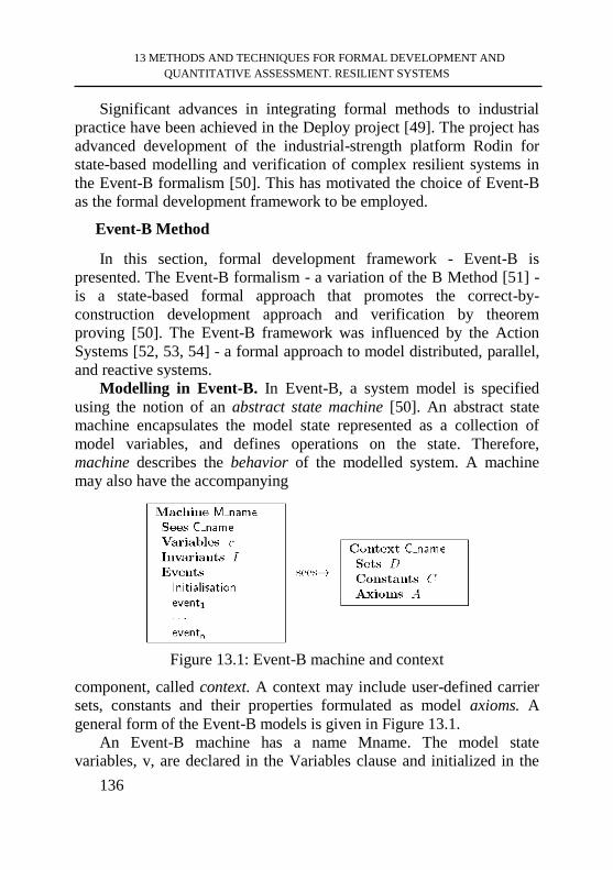
13 METHODS AND TECHNIQUES FOR FORMAL DEVELOPMENT AND

QUANTITATIVE ASSESSMENT. RESILIENT SYSTEMS

136

Significant advances in integrating formal methods to industrial

practice have been achieved in the Deploy project [49]. The project has

advanced development of the industrial-strength platform Rodin for

state-based modelling and verification of complex resilient systems in

the Event-B formalism [50]. This has motivated the choice of Event-B

as the formal development framework to be employed.

Event-B Method

In this section, formal development framework - Event-B is

presented. The Event-B formalism - a variation of the B Method [51] -

is a state-based formal approach that promotes the correct-by-

construction development approach and verification by theorem

proving [50]. The Event-B framework was influenced by the Action

Systems [52, 53, 54] - a formal approach to model distributed, parallel,

and reactive systems.

Modelling in Event-B. In Event-B, a system model is specified

using the notion of an abstract state machine [50]. An abstract state

machine encapsulates the model state represented as a collection of

model variables, and defines operations on the state. Therefore,

machine describes the behavior of the modelled system. A machine

may also have the accompanying

Figure 13.1: Event-B machine and context

component, called context. A context may include user-defined carrier

sets, constants and their properties formulated as model axioms. A

general form of the Event-B models is given in Figure 13.1.

An Event-B machine has a name Mname. The model state

variables, v, are declared in the Variables clause and initialized in the

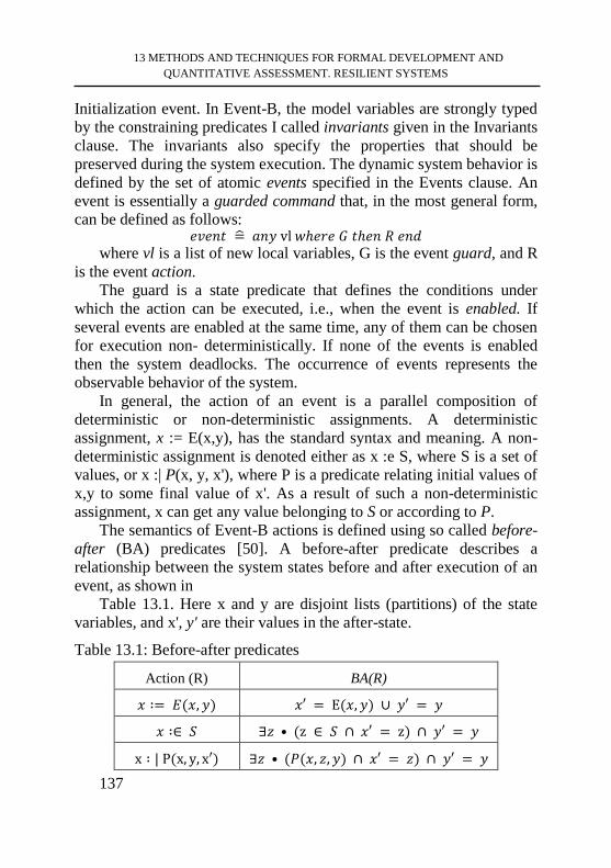
13 METHODS AND TECHNIQUES FOR FORMAL DEVELOPMENT AND

QUANTITATIVE ASSESSMENT. RESILIENT SYSTEMS

137

Initialization event. In Event-B, the model variables are strongly typed

by the constraining predicates I called invariants given in the Invariants

clause. The invariants also specify the properties that should be

preserved during the system execution. The dynamic system behavior is

defined by the set of atomic events specified in the Events clause. An

event is essentially a guarded command that, in the most general form,

can be defined as follows: 𝑒𝑣𝑒𝑛𝑡 =̂ 𝑎𝑛𝑦 vl 𝑤ℎ𝑒𝑟𝑒 𝐺 𝑡ℎ𝑒𝑛 𝑅 𝑒𝑛𝑑

where vl is a list of new local variables, G is the event guard, and R

is the event action.

The guard is a state predicate that defines the conditions under

which the action can be executed, i.e., when the event is enabled. If

several events are enabled at the same time, any of them can be chosen

for execution non- deterministically. If none of the events is enabled

then the system deadlocks. The occurrence of events represents the

observable behavior of the system.

In general, the action of an event is a parallel composition of

deterministic or non-deterministic assignments. A deterministic

assignment, x := E(x,y), has the standard syntax and meaning. A non-

deterministic assignment is denoted either as x :e S, where S is a set of

values, or x :| P(x, y, x'), where P is a predicate relating initial values of

x,y to some final value of x'. As a result of such a non-deterministic

assignment, x can get any value belonging to S or according to P.

The semantics of Event-B actions is defined using so called before-

after (BA) predicates [50]. A before-after predicate describes a

relationship between the system states before and after execution of an

event, as shown in

Table 13.1. Here x and y are disjoint lists (partitions) of the state

variables, and x', y' are their values in the after-state.

Table 13.1: Before-after predicates

Action (R) BA(R)

𝑥 ∶= 𝐸(𝑥, 𝑦) 𝑥′ = E(𝑥, 𝑦) ∪ 𝑦′ = 𝑦

𝑥 ∶∈ 𝑆 ∃𝑧 • (z ∈ 𝑆 ∩ 𝑥′ = z) ∩ 𝑦′ = 𝑦

x ∶ | P(x, y, x′) ∃𝑧 • (𝑃(𝑥, 𝑧, 𝑦) ∩ 𝑥′ = 𝑧) ∩ 𝑦′ = 𝑦

13 METHODS AND TECHNIQUES FOR FORMAL DEVELOPMENT AND

QUANTITATIVE ASSESSMENT. RESILIENT SYSTEMS

138

Event-B Refinement. Event-B employs a top-down refinement-

based approach to the system development. Development in Event-B

starts from an abstract system specification that models the most

essential functional requirements. In a sequence of refinement steps, we

gradually reduce nondeterminism and introduce detailed design

decisions. Refinement usually affects both the context and the machine.

Context refinement is a simple extension of the current context

achieved by adding new constants, sets and axioms. A machine can be

refined in two possible ways either using data refinement or

superposition refinement. In particular, we can replace abstract

variables by their concrete counterparts, i.e., perform data refinement.

In this case, the invariant of the refined machine formally defines the

relationship between the abstract and concrete variables. Via such a

gluing invariant - “refinement relation” - we mathematically establish a

correspondence between the state spaces of the refined and the abstract

machines.

During superposition refinement, new implementation details are

introduced into the system specification by means of new events and

new variables. These new events can not affect the variables of the

abstract specification and only define computations on newly

introduced variables.

The new events correspond to the stuttering steps that are not

visible at the abstract level, i.e., they refine implicit skip. To guarantee

that the refined specification preserves the global behavior of the

abstract machine, we should demonstrate that the newly introduced

events converge. To prove it, we have to define a variant - an

expression over a finite subset of natural numbers - and show that the

execution of new events decreases it. Sometimes, convergence of an

event cannot be proved due to a high level of non-determinism. In that

case, the event obtains the status anticipated. This obliges the designer

to prove, at some later refinement step, that the event indeed converges.

The correctness and consistency of Event-B models, i.e.,

verification of the model well-formedness, invariant preservation,

deadlock-freeness, correctness of the refinement steps, is demonstrated

by proving the relevant verification theorems - proof obligations. Proof

13 METHODS AND TECHNIQUES FOR FORMAL DEVELOPMENT AND

QUANTITATIVE ASSESSMENT. RESILIENT SYSTEMS

139

obligations are expressed as logical sequences, ensuring that the

transformation is performed in a correctness-preserving way [50].

Modelling, refinement and verification of Event-B models is

supported by an automated tool - Rodin platform [55]. The platform

provides the designers with an integrated modelling environment,

supports automatic generation and proving of the necessary proof

obligations by means of wide range of automated provers. Moreover,

various plug-ins created for Rodin platform allow a modeler to

transform models from one representation to another, e.g. from UML to

Event-B language [56, 57], or from Event-B specification to

programming languages C/C++ [58, 59], ADA [60, 61], etc.

The Event-B refinement process allows us to gradually introduce

implementation details, while proving preservation of functional

correctness. Such an approach seamlessly weaves verification into the

model development and allows us to construct detailed models of

complex systems is highly automated incremental manner. By

providing an immediate feedback on the correctness of model

transformations, it helps us to cope with complexity of the system

development. Another important mechanism for handling complexity

of formal development is decomposition. Model decomposition helps

the designers to separate component development from the overall

system model but ensure that the components can be recomposed into

overall system in a correctness-preserving way [62]. Event-B is

equipped with three forms of decomposition: shared-variable [63, 64,

65], shared-event [65] and modularization [66], all of which are

supported by the corresponding Rodin plug-ins [67, 68]. In this section

we rely on a modularization extension of Event B [66].

Modularization. Modularization extension allows the designers to

decompose a system into modules. Modules are components containing

groups of callable atomic operations [66, 68]. Modules may have their

own (external and internal) state and invariant properties. In general,

they can be developed separately and then composed with the main

system, when needed. Since decomposition is a special kind of

refinement, such a model transformation is also a correctness-

preserving step that has to be proven by discharging the relevant proof

obligations.

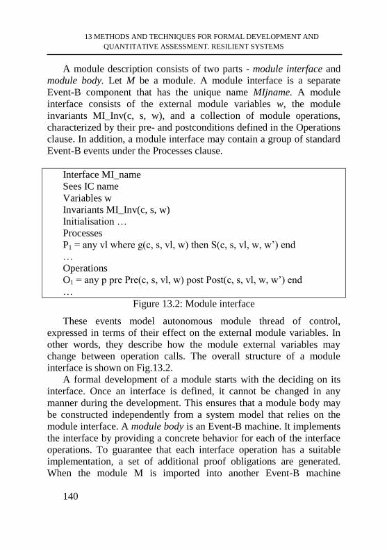
13 METHODS AND TECHNIQUES FOR FORMAL DEVELOPMENT AND

QUANTITATIVE ASSESSMENT. RESILIENT SYSTEMS

140

A module description consists of two parts - module interface and

module body. Let M be a module. A module interface is a separate

Event-B component that has the unique name MIjname. A module

interface consists of the external module variables w, the module

invariants MI_Inv(c, s, w), and a collection of module operations,

characterized by their pre- and postconditions defined in the Operations

clause. In addition, a module interface may contain a group of standard

Event-B events under the Processes clause.

Interface MI_name

Sees IC name

Variables w

Invariants MI_Inv(c, s, w)

Initialisation …

Processes

P1 = any vl where g(c, s, vl, w) then S(c, s, vl, w, w’) end

…

Operations

O1 = any p pre Pre(c, s, vl, w) post Post(c, s, vl, w, w’) end

…

Figure 13.2: Module interface

These events model autonomous module thread of control,

expressed in terms of their effect on the external module variables. In

other words, they describe how the module external variables may

change between operation calls. The overall structure of a module

interface is shown on Fig.13.2.

A formal development of a module starts with the deciding on its

interface. Once an interface is defined, it cannot be changed in any

manner during the development. This ensures that a module body may

be constructed independently from a system model that relies on the

module interface. A module body is an Event-B machine. It implements

the interface by providing a concrete behavior for each of the interface

operations. To guarantee that each interface operation has a suitable

implementation, a set of additional proof obligations are generated.

When the module M is imported into another Event-B machine

13 METHODS AND TECHNIQUES FOR FORMAL DEVELOPMENT AND

QUANTITATIVE ASSESSMENT. RESILIENT SYSTEMS

141

(specified by a special clause Uses), the importing machine may invoke

the operations of M and read the external variables of M.

We can create several instances of the given module and import

them into the same machine. Different instances of a module operate on

disjoint state spaces. Identifier prefixes can be supplied in the Uses

clause of the importing machine to distinguish the variables and the

operations of different module instances or those of the importing

machine and the imported module. Alternatively, the pre-defined

constant set can be supplied as a additional parameter. In the latter case,

module instances are created for each element of the given set, thus

producing an indexed collection (array) of module instances. A detailed

description of indexed modules is given in [69].

The modularization extension of Event-B facilitates formal

development of complex systems by allowing the designers to

decompose large specifications into separate components and verify

system-level properties at the architectural level. As a result, proof-

based verification as well as reliance on abstraction and decomposition

adopted in Event-B offers the designers a scalable support for the

development of complex distributed systems.

Quantitative Assessment

Formal modelling in Event-B allows the designers to derive

complex system architecture, formulate and prove logical system

properties and formally verify correctness of the system behavior.

While functional correctness constitutes an important aspect of

resilience, we also need to provide the developers with techniques for

quantitative resilience assessment. Quantitative assessment plays an

important role in the process of resilient system development because it

allows the developers to predict the impact of changes on such vital

aspects as, e.g., reliability and performance. Moreover, quantitative

analysis helps to find suitable trade-offs between these properties as

well as evaluate the impact of different architectural alternatives on

system resilience. Therefore, we investigate possibility of integration of

formal development in Event-B with quantitative resilience assessment.

In particular, we study integration with the probabilistic symbolic

13 METHODS AND TECHNIQUES FOR FORMAL DEVELOPMENT AND

QUANTITATIVE ASSESSMENT. RESILIENT SYSTEMS

142

model checker PRISM [70], and discrete event simulation in

SimPy[71].

PRISM model checker

PRISM model checker [70] is one of the leading software tool for

formal modelling and verification of systems that exhibit probabilistic

behavior. It provides support for analysis of three types of Markov

process - discrete time Markov chains (DTMC), continuous-time

Markov chains (CTMC) and Markov decision processes (MDP).

Additionally, it supports modelling of (priced) probabilistic timed

automata and st7]ochastic games (as a generalization of MDP) [72].

The state-based modelling language of PRISM relies on the reactive

modules formalism [.

A PRISM model consists of a number of modules which can

interact with each other. The behavior of each module is described by a

set of guarded commands that are quite similar to Event-B events. The

latter fact significantly simplifies transformation of Event-B machines

to the corresponding PRISM specifications.

While analyzing a PRISM model, one can define a number of

temporal logic properties to be evaluated by the tool. To assess

resilience, we can rely on verifying the time-bounded reachability and

reward properties. In the property specification language of PRISM,

they can be formulated using the supported temporal logics - PCTL

(Probabilistic Computation Tree Logic) [73] for discrete-time models

and CSL (Continuous Stochastic Logic) [74, 75] for continuous-time

models.

Similarly to Event-B, the PRISM language is a high-level state-

based modelling language. Essentially, PRISM supports the use of

constants and variables. The variables in PRISM are finite-ranged and

strongly typed. They also can be global or local, i.e., associated with a

particular module.

A PRISM specification is constructed as a parallel composition of

modules that can be synchronized using the standard CSP parallel

composition. In addition to local variables, each module has a number

of guarded commands that determine its dynamic behavior. Each

command consists of a guard and one or more updates over local and

13 METHODS AND TECHNIQUES FOR FORMAL DEVELOPMENT AND

QUANTITATIVE ASSESSMENT. RESILIENT SYSTEMS

143

global system variables. Each update is annotated with a probabilistic

weight (in discrete-time models) or rate (in continuous-time models).

Similarly to events in Event-B, a guarded command can be executed

(i.e., is enabled) only if its guards evaluate to TRUE. If several guarded

commands are enabled at the same time, then the choice between them

is defined by the model type - it is non-deterministic for MDP models,

probabilistic for DTMC models or modelled as an (exponential) race

condition for CTMC models.

PRISM tool has been successfully employed in many domains

including distributed coordination algorithms, wireless communication

protocols, security as well as dependability and biological models.

To enable probabilistic analysis of Event-B models in PRISM, we

rely on the continuous-time probabilistic extension of the Event-B

framework [76, 77]. This extension allows us to annotate actions of all

model events with real-valued rates and then transform a

probabilistically augmented Event-B specification into a continuous-

time Markov chain. It also implicitly introduces the notion of time into

Event-B models: for any state, the sum of action rates of all enabled in

these state events defines a parameter of the exponentially distributed

time delay that takes place before some enabled action is triggered.

Discrete-event simulation

Due to similarity between PRISM and Event-B languages, the

translation from a Event-B model to a PRISM specification is rather

straightforward. It makes the use of PRISM model checker attractive

for the performing quantitative assessment. However, the model

checking technique does not always scale to large applications. In such

case, simulation offers a viable alternative for quantitative analysis of

resilience.

Traditionally, simulation is called the process of imitating how an

actual system behaves over time [78]. A simulation generates an

artificial system history, thereby enabling analysis of system general

behavior. Simulation is built around the notion of event - an occurrence

that changes the state of the system. The system state variables are

viewed as a collection of all information that is required to define what

is happening within the system at a given moment of time.

13 METHODS AND TECHNIQUES FOR FORMAL DEVELOPMENT AND

QUANTITATIVE ASSESSMENT. RESILIENT SYSTEMS

144

A widely-used type of simulation is known as discrete-event

simulation (DES). In a DES, system state remains constant over an

interval of time between two consecutive events. Thus events signify

occurrences that change the system state. Events can be classified as

either internal or external. Internal events occur within the modelled

system, while external events occur outside the system, but still might

affect it. A simulation is run by a mechanism that repeatedly moves

simulated time forward to the starting time of the next scheduled event,

until there are no more events [79].

From the architectural perspective, a DES system consists of a

number of entities (e.g., components, processes, agents, etc.), which are

either producers or recipients of discrete events. Static entities (e.g.,

queues, buffers, etc.) can often be represented as resources. Resources

have limited availability, leading to competition among entities.

Waiting for a particular event to occur can lead to a delay, lasting for an

indefinite amount of time. In other cases, the time estimate may be

known in advance. Events can be also interrupted and pre-empted, e.g.,

in reaction to component failures or pre-defined high-priority events.

There are four primary simulation paradigms [78]: process-

interaction, event-scheduling, activity scanning, and the three-phase

method. We use SimPy [71] - a simulation framework based on

process- interaction in Python. Essentially, SimPy is a discrete-event

simulation library written in Python. The behaviour of active entities

(e.g., customers, requests) is modelled by means of processes. All

processes settle in an environment and interact with the environment

and with each other via events.

Processes are described by simple Python generators. During their

lifetime, they create events and yield them in order to wait for them to

be triggered. When a process yields an event, the process gets

suspended. SimPy resumes the process, when the event occurs. Timeout

is an important event type. Events of this type are triggered after a

certain amount of (simulated) time has passed. SimPy also provides

various types of shared resources to model limited capacity congestion

points (like servers, queues, buffers, etc.).

Discrete-event simulation represents an attractive technique for

quantitative evaluation of different system characteristics. It allows the

13 METHODS AND TECHNIQUES FOR FORMAL DEVELOPMENT AND

QUANTITATIVE ASSESSMENT. RESILIENT SYSTEMS

145

designers to perform various “what-if” type of analysis that

demonstrates sensitivity of the service architecture to changes of its

parameters. For instance, it gives an understanding on how the system

reacts on peak-loads, how adding new resources affects its

performance, what are the relationships between the degree of

redundancy and fault tolerance, etc. Moreover, while simulating the

behavior, the designers can also obtain the information on which

parameters should be monitored at run-time to optimize a resource allo-

cation strategy. However, to obtain all the above-mentioned benefits,

the designers have to ensure that the simulation models are correct and

indeed representative of the actual system. In particular, this can be

achievable via integration of simulation technique with formal

modelling.

Advancement questions

1. What is the concept of the System Resilience?

2. Explain the concept of Dependability and name its key attributes.

3. What are the four main techniques on which engineering

dependable systems are able to rely?

4. Why Goal-Based Development is crucial for software

engineering? p. 133

5. What does agent concept provide us?

6. What is the concept of the System Autonomy and

Reconfiguration and what were the reasons (motives) to remove

humans from the control?

7. What is the main idea behind the formal modelling and what are

its main approaches?

8. Explain the process of modelling in Event-B method

9.What are the two possible ways of Event-B Refinement ?

13 METHODS AND TECHNIQUES FOR FORMAL DEVELOPMENT AND

QUANTITATIVE ASSESSMENT. RESILIENT SYSTEMS

146

10. What is the role of Quantitative Assessment and what are the

tools to integrate Event-B method with quantitative resilience

assessment?

REFERENCE

1. Pereverzeva Inna Formal Development of Resilient Distributed

Systems / Inna Pereverzeva // PhD diss., Turku Centre for

Computer Science, Abo Akademi University, Faculty of

Science and Engineering, Joukahaisenkatu, Turku, Finland. –

2015.

2. Laprie J.-C. Resilience for the Scalability of Dependability : In

Fourth IEEE International Symposium on Network Computing

and Applications / J.-C. Laprie // IEEE .-2005

3. Laprie J.-C. From Dependability to Resilience / J.-C. Laprie //

IEEE Computer Society .- 2008.

4. Strigini L. Resilience: What is it, and how much do we want? /

L. Strigini // IEEE Security & Privacy .- 2012 .-10(3) .-72-75

5. Avizienis A. Basic Concepts and Taxonomy of Dependable and

Secure Computing / A. Avizienis, J.-C. Laprie, B. Randell, and

C. E. Landwehr // IEEE Trans. Dependable Sec. Comput.-

2004.-1(1).-11–33

6. Avizienis A. Dependability and its Threats - A taxonomy: In

IFIP Congress Topical Sessions / A. Avizienis, J.-C. Laprie,

and B. Randell .-2004.- pages 91– 120

7. Guelfi N. An Introduction to Software Engineering and Fault

Tolerance, chapter Software Engineering of Fault Tolerant

Systems / N. Guelfi, P. Pelliccione, H. Muccini, and A.

Romanovsky // Series on Software Engineering and Knowledge

Eng.- 2007

13 METHODS AND TECHNIQUES FOR FORMAL DEVELOPMENT AND

QUANTITATIVE ASSESSMENT. RESILIENT SYSTEMS

147

8. Lamsweerde Axel van. Goal-oriented requirements

engineering: A guided tour / Axel van Lamsweerde // In

Requirements Engineering.- 2001.- pages 249–263

9. Lamsweerde Axel van. Requirements Engineering: From

System Goals to UML Models to Software Specifications /

Axel van Lamsweerde // Wiley.-2009.

10. Lamsweerde A. van From system goals to software

architecture. In Formal Methods for Software Architectures,

Third International School on Formal Methods for the Design

of Computer, Communication and Software Systems: Software

Architectures / A. van Lamsweerde .- Bertinoro, Italy :

Springer.- September 22-27 .-2003 .- pages 25–43.

11. Franklin S. Is it an agent, or just a program?: A taxonomy for

autonomous agents: In Proceedings of the Workshop on

Intelligent Agents III, Agent Theories, Architectures, and

Languages, ECAI ’96 / S. Franklin and A. Graesser // Springer-

Verlag.- 1997.- pages 21–35.

12. Ferber J. Multi-Agent Systems: An Introduction to Distributed

Artificial Intelligence / J. Ferber.- Boston, MA, USA: Addison-

Wesley Longman Publishing Co., Inc.- 1999.-1st edition .

13. Jennings N. R. On agent-based software engineering / N. R.

Jennings // Artif. Intell.-2000.- 117(2).-277–296.

14. OMG Mobile Agents Facility (MASIF): http://www.omg.org.

15. Kephart J. O. The vision of autonomic computing / J. O.

Kephart and D. M. Chess // IEEE Computer.-2003. -36(1).-41–

50.

16. Fisher M. Verifying autonomous systems / M. Fisher, L. A.

Dennis, and M. P. Webster // Commun. ACM .- 2013.-56(9).-

84–93

13 METHODS AND TECHNIQUES FOR FORMAL DEVELOPMENT AND

QUANTITATIVE ASSESSMENT. RESILIENT SYSTEMS

148

17. Dennis L. A. Reconfigurable autonomy / L. A. Dennis, M.

Fisher, J. M. Aitken, S. M. Veres, Y. Gao, A. Shaukat, and G.

Burroughes // KI .- 2014.- 28(3).-199–207

18. Huebscher M. C. A survey of autonomic computing - degrees,

models, and applications / M. C. Huebscher and J. A. McCann

// ACM Comput. Surv.- 2008.-40(3),

19. RushbyJ. Formal methods and the certification of critical

systems: Technical Report SRI-CSL-93-7 / J. Rushby //

Computer Science Laboratory, SRI International.- 1993

20. The HOL System : online at

http://www.cl.cam.ac.uk/research/hvg/HOL/.

21. NipkowT. Isabelle/HOL — A Proof Assistant for Higher-Order

Logic: volume 2283 of LNCS / T. Nipkow, L. C. Paulson, and

M. Wenzel // Springer .- 2002

22. Coq. The Coq Proof Assistant: online at

https://coq.inria.fr/what-iscoq

23. Owre S. PVS: A prototype verification system: In Automated

Deduction - CADE-11, 11th International Conference on

Automated Deduction /S. Owre, J. M. Rushby, and N. Shankar

// Saratoga Springs, Springer.- NY, USA.- June 15-18.- 1992,

pages 748–752

24. Owre S. PVS: combining specification, proof checking, and

model checking / S. Owre, S. Rajan, J. M. Rushby, N. Shankar,

and M. K. Srivas .-New Brunswick, NJ, USA : In Computer

Aided Verification, 8th International Conference, CAV ’96,

Springer.- July 31 - August 3.-1996 pages 411–414

25. Mendon¸ca de Moura L. Z3: an efficient SMT solver. In Tools

and Algorithms for the Construction and Analysis of Systems,

14th International Conference, TACAS 2008, Held as Part of

the Joint European Conferences on Theory and Practice of

Software, ETAPS 2008 / L. Mendon¸ca de Moura and N.

13 METHODS AND TECHNIQUES FOR FORMAL DEVELOPMENT AND

QUANTITATIVE ASSESSMENT. RESILIENT SYSTEMS

149

Bjørner.- Budapest, Hungary: Springer.- March 29-April 6.-

2008 .-pages 337– 340

26. Barrett C. CVC3. In Werner Damm and Holger Hermanns,

editors, Proceedings of the 19th International Conference on

Computer Aided Verification (CAV ’07): volume 4590 of

Lecture Notes in Computer Science / C. Barrett and C. Tinelli.-

Berlin, Germany: Springer-Verlag.- 2007.- pages 298–302

27. Stump A. A decision procedure for an extensional theory of

arrays:In Proceedings of the 16th IEEE Symposium on Logic in

Computer Science (LICS ’01) / A. Stump, D. L. Dill, C. W.

Barrett, and J. Levitt .- Boston, Massachusetts :IEEE Computer

Society.- 2001 .- pages 29–37

28. Berezin S. A practical approach to partial functions in CVC

Lite. In Selected Papers from the Workshops on Disproving and

the Second International Workshop on Pragmatics of Decision

Procedures (PDPAR ’04), volume 125(3) of Electronic Notes in

Theoretical Computer Science / S. Berezin, C. Barrett, I.

Shikanian, M. Chechik, A. Gurfinkel, and D. L. Dill // Elsevier

.- 2005.-pages 13–23

29. Riazanov A. Vampire. In Automated Deduction - CADE-16,

16th International Conference on Automated Deduction :

Proceedings, volume 1632 of Lecture Notes in Computer

Science / A. Riazanov and A. Voronkov.- Trento, Italy:

Springer.- 1999 .-pages 292–296.

30. Riazanov A. The design and implementation of VAMPIRE / A.

Riazanov and A. Voronkov // AI Commun.- 2002.-15(2-3).-91–

110

31. Baier C. Principles of Model Checking / C. Baier and J.-P.

Katoen // MIT press.- 2008

13 METHODS AND TECHNIQUES FOR FORMAL DEVELOPMENT AND

QUANTITATIVE ASSESSMENT. RESILIENT SYSTEMS

150

32. Clarke E. M. The birth of model checking. In 25 Years of

Model Checking - History, Achievements, Perspectives / E. M.

Clarke // SpringerVerlag Berlin Heidelberg.- 2008.-pages 1–26.

33. Holzmann G. J. The model checker SPIN. /G. J. Holzmann//

IEEE Trans. Software Eng.- 1997.-23(5).-79–295

34. Holzmann G. J. The SPIN Model Checker - primer and

reference manual. /G. J. Holzmann. //Addison-Wesley.-2004.

35. Bernardo M. Formal Methods for the Design of Real-Time

Systems/M. Bernardo, F. Corradini, and K. G. Larsen,

editors//volume 3185 of Lecture Notes in Computer Science:

Springer .-2004.

36. The ProB Animator and Model Checker:online at

http://www.stups.uni-duesseldorf.de/ProB/index.php5/.

37. PRISM. Probabilistic Symbolic Model Checker. online at

http://www.prismmodelchecker.org/.

38. Woodcock J. C. Formal methods: Practice and Experience/J. C.

Woodcock, P. G. Larsen, J. Bicarregui, and J. S. Fitzgerald.//

ACM Comput. Surv.- 2009.-41(4)

39. Badeau F. Using B as a high level programming language in an

industrial project: Roissy VAL. /F. Badeau and A. Amelot.//In

Formal Specification and Development, 4th International

Conference.-Guildford:Springer .-2005.- pages 334–354

40. Industrial Use of the B Method.: http://www.methode-

b.com/wpcontent/uploads/2012/08/ClearSy-Industrial Use of

B1.pdf.

41. Behm P. A successful application of B in a large project. /P.

Behm, P. Benoit, A. Faivre, and J.-M. Meynadier. M´et´eor //In

FM’99 - Formal Methods, World Congress on Formal Methods

in the Development of Computing Systems.- France: Springer.-

1999.-pages 369–387.

13 METHODS AND TECHNIQUES FOR FORMAL DEVELOPMENT AND

QUANTITATIVE ASSESSMENT. RESILIENT SYSTEMS

151

42. S. P Miller. Specifying the mode logic of a flight guidance

system in core and scr. /S. P Miller. // In Proceedings of the 2nd

Workshop on Formal Methods in Software Practice, volume

4916 of Lecture Notes in Computer Science:ACM.- 1998.-page

44–53.

43. Esteve M.-A. Formal correctness, safety, dependability, and

performance analysis of a satellite. /M.-A. Esteve, J.-P. Katoen,

V. Y. Nguyen, B. Postma, and Y. Yushtein.//In Proceedings of

the 34th International Conference on Software

Engineering:Piscataway.-2012.- pages 1022–1031,

44. Rushby J. M. Analyzing cockpit interfaces using formal

methods. /J. M. Rushby.//Electr. Notes Theor. Comput. Sci..-

2001.-43.-1–14

45. H¨orl J. Formal specification of a voice communication system

used in air traffic control./J. H¨orl and B. K. Aichernig. //In

FM’99 - Formal Methods, World Congress on Formal Methods

in the Development of Computing Systems: Springer.- 1999.-

page 1868

46. Bacherini S. A story about formal methods adoption by a

railway signaling manufacturer. S. Bacherini, A. Fantechi,

M.Tempestini, and N.Zingoni. In Formal Methods, 14th

International Symposium on Formal Methods, volume 4085 of

Lecture Notes in Computer Science:Springer .-2006.-pages

179–189

47. Bowen J. Safety-critical systems, formal methods and

standards. Software Engineering Journal/J. Bowen and V.

Stavridou.-1993. -8(4).-189–209.

48. Praful Jetley R. A case study on applying formal methods to

medical devices: computer-aided resuscitation algorithm /R.

Praful Jetley, C. Carlos, and S. Purushothaman Iyer //STTT.-

2004.-5(4).-320–330.

13 METHODS AND TECHNIQUES FOR FORMAL DEVELOPMENT AND

QUANTITATIVE ASSESSMENT. RESILIENT SYSTEMS

152

49. Industrial Deployment of System Engineering Methods

Providing High Dependability and Productivity (DEPLOY).

IST FP7 IP Project: online at http://www.deploy-project.eu/.

50. J.-R. Abrial Modeling in Event-B. / J.-R. Abrial.-Cambridge

University Press.- 2010

51. Abrial J.-R. The B-Book: Assigning Programs to Meanings. /J.-

R. Abrial.-Cambridge University Press.-2005

52. Back R. J. R. Decentralization of Process Nets with Centralized

Control. / J. R. Back and R. Kurki-Suonio //In ACM SIGACT-

SIGOPS Symposium on Principles of Distributed Computing.-

1983.- pages 131–142

53. Back R. J. R. Stepwise Refinement of Action Systems.

Structured Programming/R. J. R. Back and K. Sere.-1991.-

12(1).-17–30

54. Back R. J. R. From Action Systems to Modular Systems.

Software – Concepts and Tools/R. J. R. Back and K. Sere.-

1996.-17(1).-26–39

55. Rodin. Event-B Platform:online at http://www.event-b.org/.

56. Snook C. F. UML-B: formal modeling and design aided by

UML. ACM Trans./C. F. Snook and M. J. Butler.// Softw. Eng.

Methodol.- 2006.-15(1).-92–122

57. M. Y. Said, M. J. Butler, and C. F. Snook. Language and tool

support for class and state machine refinement in UML-B. /M.

Y. Said, M. J. Butler, and C. F. Snook.//volume 5850 of

Lecture Notes in Computer Science:Springer.- 2009.-pages

579–595

58. M´ery D. Automatic code generation from event-b models./ D.

M´ery and N. K. Singh. // In Proceedings of the Second

Symposium on Information and Communication

Technology:ACM.- 2011.-pages 179–188

13 METHODS AND TECHNIQUES FOR FORMAL DEVELOPMENT AND

QUANTITATIVE ASSESSMENT. RESILIENT SYSTEMS

153

59. Mery D. Transforming event b models into verified c#

implementations. /D. Mery and R. Monahan. //In Alexei Lisitsa

and Andrei Nemytykh, editors, VPT 2013, volume 16 of EPiC

Series .-2013.-pages 57–73

60. Edmunds A. Formal modelling for ada implementations:

Tasking event-b./A. Edmunds, A. Rezazadeh, and M. J.

Butler.// In Reliable Software Technologies International

Conference on Reliable Software Technologies: Springer.-

2012.-pages 119–132

61. Edmunds A. Templates for event-b code generation. / A.

Edmunds.//In Abstract State Machines, Lecture Notes in

Computer Science.- France:Springer.- 2014.-pages 284–289

62. Hoang T. S. A survey on event-b decomposition./ T. S. Hoang,

A. Iliasov, R.Silva, and W. Wei.//ECEASST.- 2011.-46

63. Abrial J.-R. Refinement, decomposition, and instantiation of

discrete models: Application to event-b. Fundam./J.-R. Abrial

and S. Hallerstede.// Inform.- 2007.-77(1-2).-1–28

64. Hoang T. S. Event-b decomposition for parallel programs. /T.

S. Hoang and J.-R. Abrial.//In Abstract State Machines,Second

International Conference.- Canada : Proceedings.-2010. -pages

319–333

65. Butler. M. J. Decomposition structures for event-b./M. J.

Butler// In Integrated Formal Methods, 7th International

Conference.-Germany:Du¨sseldorf.- 2009. -pages 20–38

66. Iliasov A. Supporting Reuse in Event B Development:

Modularisation Approach./A. Iliasov, E. Troubitsyna, L.

Laibinis, A. Romanovsky, K. Varpaaniemi, D. Ilic, and T.

Latvala.// In Proceedings of Abstract State Machines:Springer.-

2010.- pages 174–188.

13 METHODS AND TECHNIQUES FOR FORMAL DEVELOPMENT AND

QUANTITATIVE ASSESSMENT. RESILIENT SYSTEMS

154

67. Silva R. Decomposition tool for event-b. /R. Silva, C. Pascal, T.

S. Hoang, and M. J. Butler //Softw., Pract. Exper.- 2011.-

41(2).-199–208.

68. RODIN Modularisation Plug-in: Documentation at

http://wiki.eventb.org/index.php/Modularisation Plug-in.

69. Iliasov A. Support of Indexed Modules in Event-B. /A. Iliasov,

L. Laibinis, E. Troubitsyna, and A. Romanovsky.//In

Proceedings of the 4th Rodin User and Developer

Workshop:TUCS Lecture Notes.- 2013 .-pages 29–30.

70. Kwiatkowska M. PRISM 4.0: Verification of Probabilistic

Real-time Systems./ M. Kwiatkowska, G. Norman, and D.

Parker// In CAV’11, International Conference on Computer

Aided Verification:Springer.- 2011.-pages 585–591.

71. SimPy. Simulation framework in Python:online at

http://simpy.readthedocs.org/.

72. Kwiatkowska M. Advances in Probabilistic Model Checking./

M. Kwiatkowska and D. Parker// In T. Nipkow, O. Grumberg,

and B. Hauptmann, editors, Software Safety and Security -

Tools for Analysis and Verification, volume 33 of NATO

Science for Peace and Security Series - D: Information and

Communication Security:IOS Press.- 2012.-pages 126–151

73. Hansson H. A Logic for Reasoning about Time and Reliability

/ H. Hansson and B. Jonsson// In Formal Aspects of

Computing.-1994.-pages 512–535

74. Aziz A. Verifying Continuous Time Markov Chains./A. Aziz,

K. Sanwal, V. Singhal, and R. Brayton. // In CAV’96,

International Conference on Computer Aided

Verification:Springer.-1996.-pages 269–276

75. Baier C. Approximate Symbolic Model Checking of

Continuous-Time Markov Chains/C. Baier, J.-P. Katoen, and

13 METHODS AND TECHNIQUES FOR FORMAL DEVELOPMENT AND

QUANTITATIVE ASSESSMENT. RESILIENT SYSTEMS

155

H. Hermanns. // In CONCUR’99, International Conference on

Concurrency Theory:Springer.-.-pages 146–161

76. Tarasyuk A. Formal Modelling and Verification of Service-

Oriented Systems in Probabilistic Event-B/ A. Tarasyuk, E.

Troubitsyna, and L. Laibinis.// In IFM 2012, Integrated Formal

Methods:Springer.-2012.-pages 237–252

77. Tarasyuk A. Integrating stochastic reasoning into event-b

development. /A. Tarasyuk, E. Troubitsyna, and L. Laibinis.

//Formal Asp. Comput.- 2015.-27(1).-53– 77

78. Schriber T. J. How discrete-event simulation software works. /

T. J. Schriber and D. T. Brunner.//In Jerry Banks, editor,

Handbook of Simulation,John Wiley & Sons .-2007.- pages

765–812.

14 FORMAL DEVELOPMENT AND QUANTITATIVE ASSESSMENT OF RESILIENT

DISTRIBUTED SYSTEMS

156

CHAPTER 14. FORMAL DEVELOPMENT AND

QUANTITATIVE ASSESSMENT OF RESILIENT

DISTRIBUTED SYSTEMS

Content of the chapter 14

14.1 Overview of the Proposed ApproachОшибка! Закладка не

определена.

14.2 Resilience-Explicit Development Based on Functional

Decomposition. ....................... Ошибка! Закладка не определена.

14.3 Modelling Component Interactions with Multi-Agent

Framework .............................. Ошибка! Закладка не определена.

14.4 Goal-Oriented Modelling of Resilient SystemsОшибка! Закладка не определена.

14.5 Pattern-Based Formal Development of Resilient MASОшибка! Закладка не определена.

14.6 Formal Goal-Oriented Reasoning About Resilient Re-

configurable MAS .................. Ошибка! Закладка не определена.

14.7 Modelling and Assessment of Resilient ArchitecturesОшибка! Закладка не определена.

14 FORMAL DEVELOPMENT AND QUANTITATIVE ASSESSMENT OF RESILIENT

DISTRIBUTED SYSTEMS

157

14.1 Overview of the Proposed Approach

This chapter presents an integrated approach to development and

assessment of resilient distributed systems. Approach relies on formal

development by refinement in Event-B, which is augmented with

quantitative resilience assessment in the probabilistic model checker

PRISM and discrete event simulation in SimPy.

Unreliability of system components and communication channels,

complex component interactions as well as highly dynamic operating

conditions make the problem of developing resilient distributed systems

challenging. To address this problem, we need advanced methods that

are able to cope with the complexity inherent to such systems.

The Event-B framework relies on three main mechanisms for

coping with complexity: abstraction, decomposition and proofs.

Development of a distributed system in Event-B starts from creating an

abstract system specification (model). Often such a specification gives

a “black-box” model of the system behavior, i.e., it focuses on defining

the externally observable behavior while abstracting away from the

system component architecture and the internal functional behavior.

The initial Event-B model represents a centralized system that exhibits

the desired externally observable behavior and properties. The

following refinement steps aim at transforming the abstract model into

a detailed system specification by gradually unfolding the system

architecture, precisely defining the functional behavior as well as

deriving a detailed representation of component interactions.

In this chapter, we show how the described above generic approach

to development of distributed systems by refinement can be tailored to

support resilience-explicit development of different types of systems.

The resulting approach shares the common idea of using refinement as

the main vehicle for unfolding the system architecture and dynamics.

Refinement facilitates systematic introduction of the mechanisms for

ensuring system resilience while defining various inter-relationships

between the system elements. Moreover, since quantitative assessment

of different resilience characteristics is an essential part of the system

design for resilience, we show how Event-B models can be augmented

14 FORMAL DEVELOPMENT AND QUANTITATIVE ASSESSMENT OF RESILIENT

DISTRIBUTED SYSTEMS

158

with quantitative data and, as a result, serve as a basis for quantitative

resilience assessment.

Resilience-explicit development based on functional decomposi-

tion. To present approach, let us start first by considering the systems

that perform a predefined scenario that can be implemented by a

deterministic sequential execution flow. Such kind of the system

behavior is typical for a certain class of systems, which includes,

among others, service-oriented and control systems. In service-oriented

systems, a service can be often modelled as a sequential composition of

subservices. Such a composite service can be provided only if each

subservice is successfully executed. A similar type of reasoning can be

used for modelling control systems. Since control systems are cyclic,

each execution cycle can be represented as a sequential execution of

certain functional blocks.

In approach, let us explicitly define the resilience-explicit

refinement process for such systems. Specifically, we demonstrate that

modelling of not only the nominal system behavior but also a

possibility of system failures already at the abstract level can facilitate a

rigorous systematic derivation of the required fault tolerance

mechanisms. Then we discuss generic functional decomposition as a

refinement step that results in defining a high-level execution flow. We

explain how to establish a connection between a global system failure

and the corresponding failures in the execution flow. Further, we

demonstrate how refinement can be used for deriving the component-

based system architecture and linking component failures with those in

the system execution flow. Moreover, establishing the connection

between the functionality of the system and that of its components

allows us to systematically derive the system reconfiguration

mechanisms that are based on reallocation of execution of certain

functional tasks from the failed components to the healthy ones.

Finally, to evaluate the impact of reconfiguration on the system

performance and reliability, we augment the resulting Event-B models

defining various reconfiguration scenarios with the necessary proba-

bilistic information and demonstrate how to quantitatively assess

different reconfiguration strategies.

14 FORMAL DEVELOPMENT AND QUANTITATIVE ASSESSMENT OF RESILIENT

DISTRIBUTED SYSTEMS

159

Modelling component interactions. After presenting the generic

resilience-explicit development process for systems with a deterministic

sequential execution flow, we focus on detailed analysis of component

interactions while providing a certain function (service) or participating

in a specific collaboration. To perform the required functions while

ensuring fault tolerance, the system components should interact and

cooperate with each other. To facilitate reasoning about such

cooperative behavior, we treat components as agents and a resilient

distributed system as a multi-agent system. The multi-agent modelling

perspective helps us to define the essential properties of cooperative

agent activities. As a result, we derive the constraints that should be

imposed on agent interactions to ensure correct and safe functioning

despite component and communication failures.

Resilient-explicit goal-oriented refinement process. Another large

class of distributed systems includes the systems whose execution flow

is highly non-deterministic, with a loose connection between functional

blocks. Typical examples of such systems are standard multi-agent

systems whose components (agents) have some degree of autonomy.

For such kind of systems, it is convenient to adopt the goal-oriented

reasoning style. In the this section a development method for such

systems that formalizes the resilient-explicit goal-oriented refinement

process is proposed.

Resilience can be defined as the ability of a system to achieve its

objectives - goals - despite failures and other changes. We define a set

of specification and refinement patterns that reflect the main concepts

of the goal-oriented development. The refinement approach is

employed to support the goal decomposition process, thus allowing us

to define the system goals at different levels of abstraction. Let us

follow the same generic strategy for development of distributed goal-

oriented systems by refinement. Namely, we start by abstractly defining

system goals, then perform goal decomposition by refinement, and

finally introduce a representation of system agents, whose collaborative

activities ensure goal reachability. Therefore, resilience-explicit goal-

oriented refinement approach aims at ensuring goal reachability “by

construction”. It allows the developers to systematically introduce the

required reconfiguration mechanisms to ensure that the system

14 FORMAL DEVELOPMENT AND QUANTITATIVE ASSESSMENT OF RESILIENT

DISTRIBUTED SYSTEMS

160

progresses towards achieving its goals despite agent failures (thereby,

address “negative” changes) or becomes more performant by using its

agents more efficiently (thereby, address “positive” changes).

We consider a dynamic reconfiguration as a powerful technique for

achieving system resilience because it allows the system to adapt to

changes by modifying its structure, inter-agent relationships and

dependencies. However, ensuring correctness of the incorporated

reconfiguration mechanisms is a complex task. To address this issue,

we formalize the possible interdependencies between goals and agents

as well as formulate the conditions for ensuring goal reachability in a

reconfigurable multi-agent system. The proposed formalization gives a

formal systematization of the introduced concepts and can be seen as

generic guidelines for designing reconfigurable systems.

In the resilience-explicit goal-oriented development approach let us

assume that the agents are sufficiently reliable, i.e., some agents will

stay operational during the whole process of goal achieving. To validate

such an assumption and derive the constraints on agents reliability, we

need to employ quantitative analysis.

Quantitative assessment is also required to evaluate the impact of

various architectural solutions on the system performance and

reliability. Integration with probabilistic model checking in PRISM

allows us to achieve these objectives. We augment Event-B models

with quantitative data and transform them into input models for the

PRISM model checker. As a result, quantitative assessment allows the

designers to make informed design choices and develop systems with

predictable resilience characteristics.

Modelling and assessment of resilient architectures Finally, in the

last part of this chapter, we investigate how a resilient-explicit

refinement approach can be adopted to derive distributed architectures

with the incorporated fault tolerance mechanisms. Let us consider a

particular approach to ensure fault tolerance - write-ahead logging

(WAL) - and experiment with deriving several alternative architectures

implementing it. Each architectural solution exhibit different reliability

and performance characteristics. Let us demonstrate how to derive

different architectures by refinement and formally define data integrity

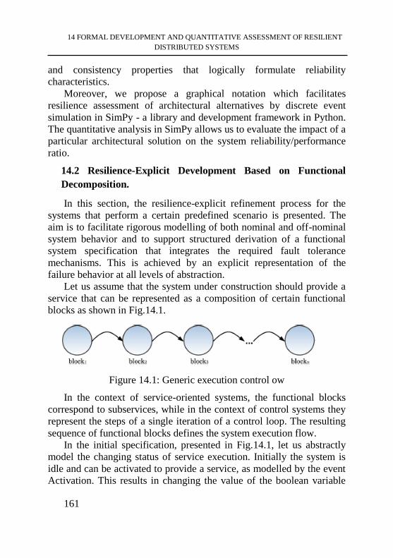
14 FORMAL DEVELOPMENT AND QUANTITATIVE ASSESSMENT OF RESILIENT

DISTRIBUTED SYSTEMS

161

and consistency properties that logically formulate reliability

characteristics.

Moreover, we propose a graphical notation which facilitates

resilience assessment of architectural alternatives by discrete event

simulation in SimPy - a library and development framework in Python.

The quantitative analysis in SimPy allows us to evaluate the impact of a

particular architectural solution on the system reliability/performance

ratio.

14.2 Resilience-Explicit Development Based on Functional

Decomposition.

In this section, the resilience-explicit refinement process for the

systems that perform a certain predefined scenario is presented. The

aim is to facilitate rigorous modelling of both nominal and off-nominal

system behavior and to support structured derivation of a functional

system specification that integrates the required fault tolerance

mechanisms. This is achieved by an explicit representation of the

failure behavior at all levels of abstraction.

Let us assume that the system under construction should provide a

service that can be represented as a composition of certain functional

blocks as shown in Fig.14.1.

Figure 14.1: Generic execution control ow

In the context of service-oriented systems, the functional blocks

correspond to subservices, while in the context of control systems they

represent the steps of a single iteration of a control loop. The resulting

sequence of functional blocks defines the system execution flow.

In the initial specification, presented in Fig.14.1, let us abstractly

model the changing status of service execution. Initially the system is

idle and can be activated to provide a service, as modelled by the event

Activation. This results in changing the value of the boolean variable

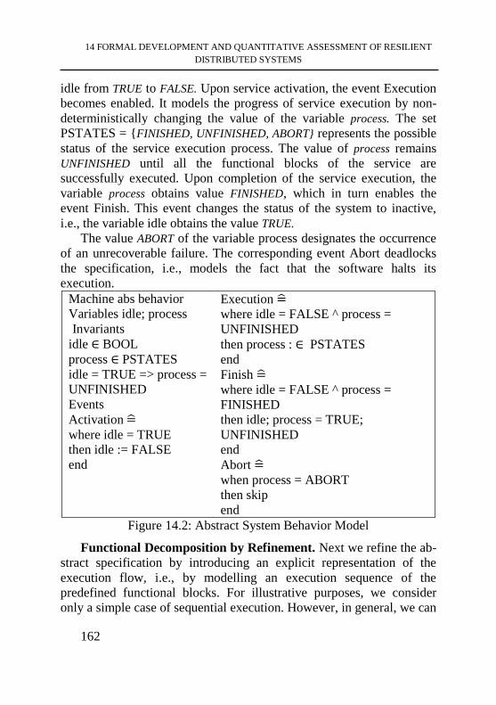
14 FORMAL DEVELOPMENT AND QUANTITATIVE ASSESSMENT OF RESILIENT

DISTRIBUTED SYSTEMS

162

idle from TRUE to FALSE. Upon service activation, the event Execution

becomes enabled. It models the progress of service execution by non-

deterministically changing the value of the variable process. The set

PSTATES = {FINISHED, UNFINISHED, ABORT} represents the possible

status of the service execution process. The value of process remains

UNFINISHED until all the functional blocks of the service are

successfully executed. Upon completion of the service execution, the

variable process obtains value FINISHED, which in turn enables the

event Finish. This event changes the status of the system to inactive,

i.e., the variable idle obtains the value TRUE.

The value ABORT of the variable process designates the occurrence

of an unrecoverable failure. The corresponding event Abort deadlocks

the specification, i.e., models the fact that the software halts its

execution.

Machine abs behavior

Variables idle; process

Invariants

idle ∈ BOOL

process ∈ PSTATES

idle = TRUE => process =

UNFINISHED

Events

Activation =̂

where idle = TRUE

then idle := FALSE

end

Execution =̂

where idle = FALSE ^ process =

UNFINISHED

then process : ∈ PSTATES

end

Finish =̂

where idle = FALSE ^ process =

FINISHED

then idle; process = TRUE;

UNFINISHED

end

Abort =̂

when process = ABORT

then skip

end

Figure 14.2: Abstract System Behavior Model

Functional Decomposition by Refinement. Next we refine the ab-

stract specification by introducing an explicit representation of the

execution flow, i.e., by modelling an execution sequence of the

predefined functional blocks. For illustrative purposes, we consider

only a simple case of sequential execution. However, in general, we can

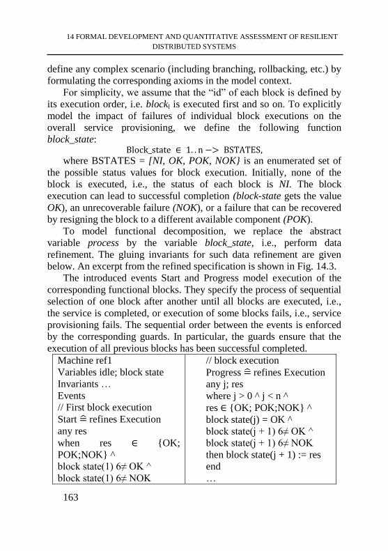
14 FORMAL DEVELOPMENT AND QUANTITATIVE ASSESSMENT OF RESILIENT

DISTRIBUTED SYSTEMS

163

define any complex scenario (including branching, rollbacking, etc.) by

formulating the corresponding axioms in the model context.

For simplicity, we assume that the “id” of each block is defined by

its execution order, i.e. blockl is executed first and so on. To explicitly

model the impact of failures of individual block executions on the

overall service provisioning, we define the following function

block_state: Block_state ∈ 1. . n −> BSTATES,

where BSTATES = [NI, OK, POK, NOK} is an enumerated set of

the possible status values for block execution. Initially, none of the

block is executed, i.e., the status of each block is NI. The block

execution can lead to successful completion (block-state gets the value

OK), an unrecoverable failure (NOK), or a failure that can be recovered

by resigning the block to a different available component (POK).

To model functional decomposition, we replace the abstract

variable process by the variable block_state, i.e., perform data

refinement. The gluing invariants for such data refinement are given

below. An excerpt from the refined specification is shown in Fig. 14.3.

The introduced events Start and Progress model execution of the

corresponding functional blocks. They specify the process of sequential

selection of one block after another until all blocks are executed, i.e.,

the service is completed, or execution of some blocks fails, i.e., service

provisioning fails. The sequential order between the events is enforced

by the corresponding guards. In particular, the guards ensure that the

execution of all previous blocks has been successful completed.

Machine ref1

Variables idle; block state

Invariants …

Events

// First block execution

Start =̂ refines Execution

any res

when res ∈ {OK;

POK;NOK} ^

block state(1) 6≠ OK ^

block state(1) 6≠ NOK

// block execution

Progress =̂ refines Execution

any j; res

where j > 0 ^ j < n ^

res ∈ {OK; POK;NOK} ^

block state(j) = OK ^

block state(j + 1) 6≠ OK ^

block state(j + 1) 6≠ NOK

then block state(j + 1) := res

end

…

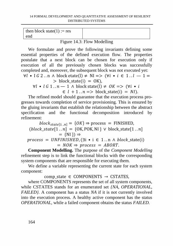
14 FORMAL DEVELOPMENT AND QUANTITATIVE ASSESSMENT OF RESILIENT

DISTRIBUTED SYSTEMS

164

then block state(1) := res

end

Figure 14.3: Flow Modelling

We formulate and prove the following invariants defining some

essential properties of the defined execution flow. The properties

postulate that a next block can be chosen for execution only if

execution of all the previously chosen blocks was successfully

completed and, moreover, the subsequent block was not executed yet:

∀𝑙 • I 𝐺 2 . . n ∧ block etate(l) ≠ NI => (∀𝑖 • 𝑖 ∈ 1 . . 𝑙 — 1 => block_state(i) = OK),

∀𝑙 • 𝑙 𝐺 1 . . 𝑛 — 1 ∧ block state(l) ≠ 𝑂𝐾 => (∀𝑖 • 𝑖 ∈ 𝑙 + 1 . . 𝑛 => block_state(i) = 𝑁𝐼).

The refined model should guarantee that the execution process pro-

gresses towards completion of service provisioning. This is ensured by

the gluing invariants that establish the relationship between the abstract

specification and the functional decomposition introduced by

refinement:

𝑏𝑙𝑜𝑐𝑘𝑠𝑡𝑎𝑡𝑒[1 ..𝑛] = {𝑂𝐾} ⇒ process = FINISHED,

(𝑏𝑙𝑜𝑐𝑘_𝑠𝑡𝑎𝑡𝑒[1 . . 𝑛] = {OK, POK, NI } ∨ block_state[1 . . 𝑛] = {NI }) ⇒

𝑝𝑟𝑜𝑐𝑒𝑠𝑠 = 𝑈𝑁𝐹𝐼𝑁𝐼𝑆𝐻𝐸𝐷, (∃i • i ∈ 1 . . n ∧ 𝑏𝑙𝑜𝑐𝑘_state(i) = 𝑁𝑂𝐾 ⇒ 𝑝𝑟𝑜𝑐𝑒𝑠𝑠 = 𝐴𝐵𝑂𝑅𝑇.

Component Modelling. The purpose of the Component Modelling

refinement step is to link the functional blocks with the corresponding

system components that are responsible for executing them.

We define a variable representing the current state for each system

component:

comp_state ∈ COMPONENTS → CSTATES, where COMPONENTS represents the set of all system components,

while CSTATES stands for an enumerated set {NA, OPERATIONAL,

FAILED}. A component has a status NA if it is not currently involved

into the execution process. A healthy active component has the status

OPERATIONAL, while a failed component obtains the status FAILED.

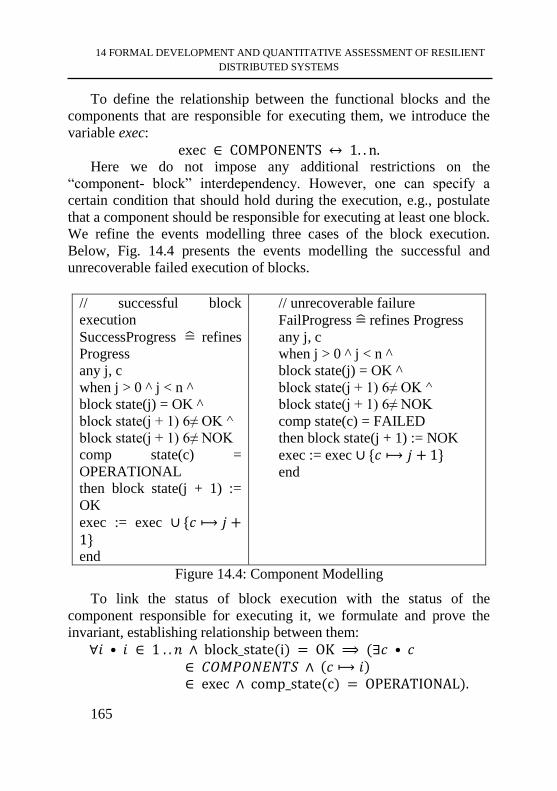
14 FORMAL DEVELOPMENT AND QUANTITATIVE ASSESSMENT OF RESILIENT

DISTRIBUTED SYSTEMS

165

To define the relationship between the functional blocks and the

components that are responsible for executing them, we introduce the

variable exec:

exec ∈ COMPONENTS ↔ 1. . n. Here we do not impose any additional restrictions on the

“component- block” interdependency. However, one can specify a

certain condition that should hold during the execution, e.g., postulate

that a component should be responsible for executing at least one block.

We refine the events modelling three cases of the block execution.

Below, Fig. 14.4 presents the events modelling the successful and

unrecoverable failed execution of blocks.

// successful block

execution

SuccessProgress =̂ refines

Progress

any j, c

when j > 0 ^ j < n ^

block state(j) = OK ^

block state(j + 1) 6≠ OK ^

block state(j + 1) 6≠ NOK

comp state(c) =

OPERATIONAL

then block state(j + 1) :=

OK

exec := exec ∪ {𝑐 ⟼ 𝑗 +1} end

// unrecoverable failure

FailProgress =̂ refines Progress

any j, c

when j > 0 ^ j < n ^

block state(j) = OK ^

block state(j + 1) 6≠ OK ^

block state(j + 1) 6≠ NOK

comp state(c) = FAILED

then block state(j + 1) := NOK

exec := exec ∪ {𝑐 ⟼ 𝑗 + 1} end

Figure 14.4: Component Modelling

To link the status of block execution with the status of the

component responsible for executing it, we formulate and prove the

invariant, establishing relationship between them:

∀𝑖 • 𝑖 ∈ 1 . . 𝑛 ∧ block_state(i) = OK ⟹ (∃𝑐 • 𝑐 ∈ 𝐶𝑂𝑀𝑃𝑂𝑁𝐸𝑁𝑇𝑆 ∧ (𝑐 ⟼ 𝑖)∈ exec ∧ comp_state(c) = OPERATIONAL).

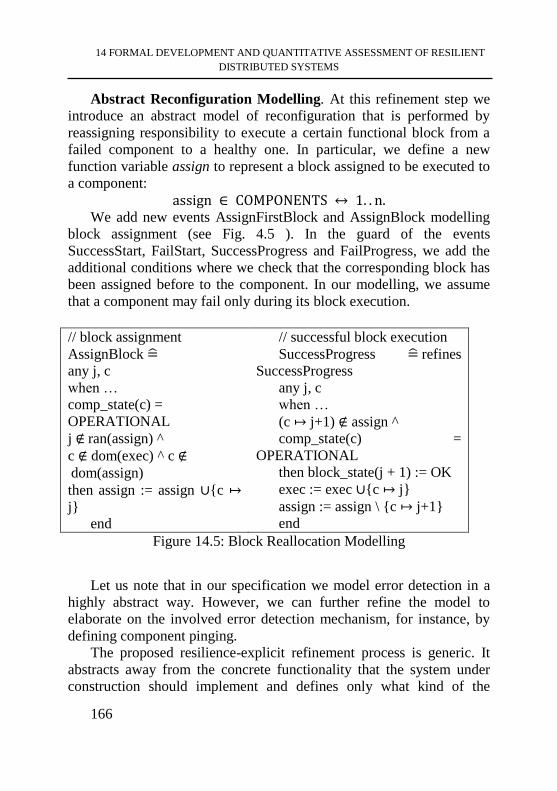
14 FORMAL DEVELOPMENT AND QUANTITATIVE ASSESSMENT OF RESILIENT

DISTRIBUTED SYSTEMS

166

Abstract Reconfiguration Modelling. At this refinement step we

introduce an abstract model of reconfiguration that is performed by

reassigning responsibility to execute a certain functional block from a

failed component to a healthy one. In particular, we define a new

function variable assign to represent a block assigned to be executed to

a component:

assign ∈ COMPONENTS ↔ 1. . n. We add new events AssignFirstBlock and AssignBlock modelling

block assignment (see Fig. 4.5 ). In the guard of the events

SuccessStart, FailStart, SuccessProgress and FailProgress, we add the

additional conditions where we check that the corresponding block has

been assigned before to the component. In our modelling, we assume

that a component may fail only during its block execution.

// block assignment

AssignBlock =̂

any j, c

when …

comp_state(c) =

OPERATIONAL

j ∉ ran(assign) ^

c ∉ dom(exec) ^ c ∉ dom(assign)

then assign := assign ∪{c ↦

j}

end

// successful block execution

SuccessProgress =̂ refines

SuccessProgress

any j, c

when …

(c ↦ j+1) ∉ assign ^

comp_state(c) =

OPERATIONAL

then block_state(j + 1) := OK

exec := exec ∪{c ↦ j}

assign := assign \ {c ↦ j+1}

end

Figure 14.5: Block Reallocation Modelling

Let us note that in our specification we model error detection in a

highly abstract way. However, we can further refine the model to

elaborate on the involved error detection mechanism, for instance, by

defining component pinging.

The proposed resilience-explicit refinement process is generic. It

abstracts away from the concrete functionality that the system under

construction should implement and defines only what kind of the

14 FORMAL DEVELOPMENT AND QUANTITATIVE ASSESSMENT OF RESILIENT

DISTRIBUTED SYSTEMS

167

refinement steps should be performed and which types of properties

that should be defined and verified. The final refinement step can be

seen as a starting point for introducing different reconfiguration

strategies and, consequently, employing quantitative assessment

technique.

Each reconfiguration alternative (i.e., a different reconfiguration

strategy or mechanism) results in creating the corresponding Event-B

model. To evaluate the impact of different reconfiguration alternatives,

we transform the models into inputs to the PRISM model checker. To

achieve this, we augment the corresponding Event-B models with the

following probabilistic data:

- the lengths of time delays required by components to execute

specific functional blocks;

- the occurrence rates of possible failures of these components.

Moreover, we replace all the local nondeterminism with the

(exponential) race conditions. Such a transformation allows us to

represent the behavior of Event-B machines by continuous time

Markov chains and use the probabilistic symbolic model checker

PRISM to evaluate reliability and performance of the proposed models.

14.3 Modelling Component Interactions with Multi-Agent

Framework

In the resilience-explicit refinement process presented above, we

abstracted away from modelling component interactions while

performing the predefined functions. Usually, execution of a certain

functional block and especially achieving fault tolerance relies on the

assumption that the components behave in a cooperative way. For

instance, when execution of a functional block is being reallocated from

a failed component to a healthy one, the healthy component needs to

accept the new responsibility, i.e. behave cooperatively.

The multi-agent modelling paradigm facilitates reasoning about the

cooperative component behavior. We adopt this paradigm to

demonstrate how to reason about resilience of complex component

interactions. It allows us to treat the components of a resilient

distributed system as agents and execution of system functions or

14 FORMAL DEVELOPMENT AND QUANTITATIVE ASSESSMENT OF RESILIENT

DISTRIBUTED SYSTEMS

168

services as cooperative agent activities. Next let us present the formal

approach to resilience-explicit modelling of agent interactions.

Let us formally reason about agents, their attributes and behavior as

well as agent cooperative activities. The formalization allow us to

establish logical connections between agents and define the conditions

under which agents interactions result in correct execution of a

cooperative activity. Moreover, the established dynamic connections

(called relationships) between agents allow us to explicitly reason

about resilience of complex agent interactions.

A multi-agent system MAS is a tuple (𝐴, 𝜇, 𝑅, 𝛴, 𝐸, 𝐴𝑐𝑡𝑖𝑣𝑒, 𝑅𝑒𝑙), where A is a set of all the system agents, 𝜇 is the system middleware, R

is a set of all possible relationships between agents in a MAS, 𝛴 is the

system state space, and E is a collection of system events (reactions).

Moreover, the dynamic system attributes Active and Rel map a given

system state to a set of the active (healthy) system agents and a set of

dynamic relationships between the active agents respectively.

The system dynamics is modelled as a set of system events E,

where each event e e E can be formally represented as a relation on

input and output system states, i.e., e : Σ ↔ Σ. The dynamic system

attributes Active and Rel are then simply functions from Σ, i.e., Active :

Σ → P(A) and Rel : Σ → P(R), returning respectively the current sets of

active system agents and dynamic relationships between them.

Intuitively, two or more system agents being in a dynamic relationship

means that these agents are currently involved in a specific

collaboration needed to provide a predefined system function or

service.

Each system agent belongs to a particular agent class. Essentially

these classes represent a partitioning of the system agents into different

groups according to their capabilities. In general, there can be many

agent classes Ai, i ∈ 1..n, such that Ai C A. We assume that all of them

are disjoint.

The system middleware μ can be considered as a special kind of the

system agent that is always present in the system. The main responsibil-

ity of the middleware is to ensure communication between different

agents, detect appearance of new agents or disappearance (both normal

14 FORMAL DEVELOPMENT AND QUANTITATIVE ASSESSMENT OF RESILIENT

DISTRIBUTED SYSTEMS

169

and abnormal) of the existing agents, recover from the situations when

the required connections between the agents are lost, etc.

The system state space Σ consists of all possible states of agents and

the middleware. The system events E then include all internal and

external system reactions (state transitions). We assume that each agent

may have a number of dynamic attributes that can be changed during

these transitions. The values of these attributes in a particular state also

determine whether a particular agent is currently “eligible”, i.e., can be

involved in execution of specific system events.

Each interaction activity between different agents (or an agent and

the middleware) may be composed of a set of events. Moreover, system

events may model appearance or disappearance of agents, sending

request from one agent to another, recovery of lost connections, etc.

A set R defines all possible dynamic relationships or connections

between agents of the same or different classes. We assume the

existence of a number of available data constructor functions to create

elements of R. More precisely, for each relationship r ∈ R, r is

modelled as a result of an application of some data constructor function

r = RConstri(𝑎1, a2, … , am),

where R_Constri : 𝐴𝑖1∗ 𝑥𝐴𝑖2

∗ …𝑥𝐴𝑖𝑚∗ ⟼ 𝑅 for some m ∈ Nl and each

𝐴𝑖𝑗∗ = Ak ∪ {? } for some agent type Ak. Here ⟼ designates an

injection function and “?” stands for an unknown agent of the

corresponding class.

A relationship can be pending, i.e., incomplete. This is indicated by

putting the question marks instead of a concrete agent, e.g.,

R_Constri(a1 , a2, ?, a4, ?). Pending relationships are often caused by

disappearance or a failure of the agents previously involved in a

relationship. Moreover, an existing active agent may initiate a new

pending relationship. Once a pending relationships is resolved

(completed), the question mark is replaced by a concrete agent.

While R represents all possible agent relationships, Rel stores the

currently active (both complete and pending) relationships. For a

relationship to be active, all the involved in it agents should be active as

well. In other words, for any σ ∈ Σ and r ∈ Rel(σ), if a concrete

agent ai is involved in r, it should be an active one, i.e., ai ∈ Active(σ).

14 FORMAL DEVELOPMENT AND QUANTITATIVE ASSESSMENT OF RESILIENT

DISTRIBUTED SYSTEMS

170

Let us now consider some expected properties that should be hold

for interactions between agents as well as between agents and the

middleware.

Property 14.1.

Let EAA and EAµ, be all interaction activities (sets of events)

defined between agents or between agents and middleware respectively.

Moreover, for each agent a ∈ A, let Ea be a set of events in which the

agent a might be involved. Then

∀𝜎, 𝑎 ∗ 𝑎 ∈ 𝐴𝑐𝑡𝑖𝑣𝑒 (σ) ⇒ Ea(σ) ∈ 𝐸𝐴𝐴 U 𝐸𝐴𝜇, 𝑎𝑛𝑑

∀σ, a ∗ 𝑎 ∉ Active (𝜎) ⇒ 𝐸𝑎(𝜎) ∈ EAμ The property restricts agent interactions with respect to the agent

activity status. For instance, this property implies that, when an agent is

recovering from a failure, it cannot be involved into any cooperative

activities with other agents. Therefore, while modelling agent

interactions, we have to take into account the agent status.

To represent such a behavior in Event-B, we define the following

events modelling agent activities with the middleware. In particular, the

events Appearance and Disappearance model joining and leaving the

system by agents (of any classes).

Appearance =̂

any a

when a ∈ AGENTS

∧ 𝑎 ∉ 𝐴𝑐𝑡𝑖𝑣𝑒 then Active := Active

∪{a} end

Disappearance =̂

any a

when a ∈ Active

then Active := Active \ {a} end

Here AGENTS defines a set of all system agents (i.e., A), while

Active represents the subset of active agents.

In a similar way, only active agents can interact with each other as

shown by the event Interaction.

Interaction =̂

any a1,a2

when a1 ∈ 𝐴𝑐𝑡𝑖𝑣𝑒 ∧ 𝑎2 ∈ 𝐴𝑐𝑡𝑖𝑣𝑒 ∧

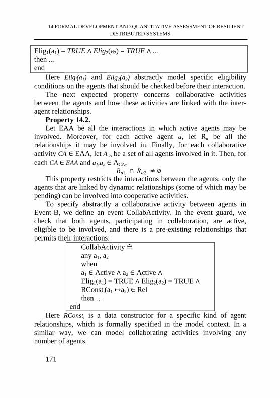
14 FORMAL DEVELOPMENT AND QUANTITATIVE ASSESSMENT OF RESILIENT

DISTRIBUTED SYSTEMS

171

Elig1(a1) = TRUE ∧ Elig2(a2) = TRUE ∧ ...

then ...

end

Here Eligl(a1) and Elig2(a2) abstractly model specific eligibility

conditions on the agents that should be checked before their interaction.

The next expected property concerns collaborative activities

between the agents and how these activities are linked with the inter-

agent relationships.

Property 14.2.

Let EAA be all the interactions in which active agents may be

involved. Moreover, for each active agent a, let Ra be all the

relationships it may be involved in. Finally, for each collaborative

activity CA ∈ EAA, let ACA be a set of all agents involved in it. Then, for

each CA ∈ EAA and a1,a2 ∈ ACA, 𝑅𝑎1 ∩ 𝑅𝑎2 ≠ ∅

This property restricts the interactions between the agents: only the

agents that are linked by dynamic relationships (some of which may be

pending) can be involved into cooperative activities.

To specify abstractly a collaborative activity between agents in

Event-B, we define an event CollabActivity. In the event guard, we

check that both agents, participating in collaboration, are active,

eligible to be involved, and there is a pre-existing relationships that

permits their interactions:

CollabActivity =̂

any a1, a2

when

a1 ∈ Active ∧ a2 ∈ Active ∧

Elig1(a1) = TRUE ∧ Elig2(a2) = TRUE ∧

RConsti(a1 ↦a2) ∈ Rel

then …

end

Here RConsti is a data constructor for a specific kind of agent

relationships, which is formally specified in the model context. In a

similar way, we can model collaborating activities involving any

number of agents.

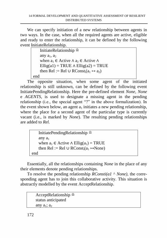
14 FORMAL DEVELOPMENT AND QUANTITATIVE ASSESSMENT OF RESILIENT

DISTRIBUTED SYSTEMS

172

We can specify initiation of a new relationship between agents in

two ways. In the case, when all the required agents are active, eligible

and ready to enter the relationship, it can be defined by the following

event InitiateRelationship.

InitiateRelationship =̂

any a1, a2

when a1 ∈ Active ∧ a2 ∈ Active ∧

Ellig(a1) = TRUE ∧ Ellig(a2) = TRUE

then Rel := Rel ∪ RConsti(a1 ↦ a2)

end

The opposite situation, when some agent of the initiated

relationship is still unknown, can be defined by the following event

InitiatePendingRelationship. Here the pre-defined element None, None

e AGENTS, is used to designate a missing agent in the pending

relationship (i.e., the special agent “?” in the above formalization). In

the event shown below, an agent a1 initiates a new pending relationship,

where the place for a second agent of the particular type is currently

vacant (i.e., is marked by None). The resulting pending relationships

are added to Rel.

InitiatePendingRelationship =̂

any a1

when a1 ∈ Active ∧ Ellig(a1) = TRUE

then Rel := Rel ∪ RConsti(a1 ↦None)

end

Essentially, all the relationships containing None in the place of any

their elements denote pending relationships.

To resolve the pending relationship RConsti(a1 ^ None), the corre-

sponding agent has to join this collaborative activity. This situation is

abstractly modelled by the event AcceptRelationship.

AcceptRelationship =̂

status anticipated

any a1; a2

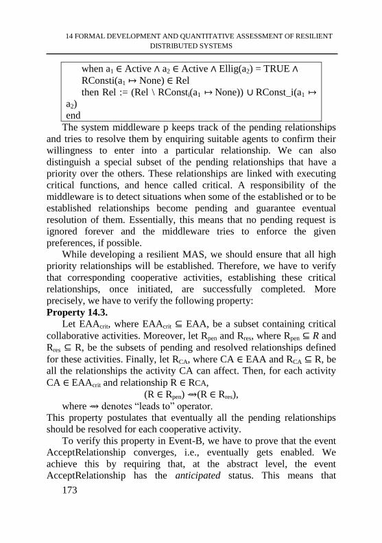
14 FORMAL DEVELOPMENT AND QUANTITATIVE ASSESSMENT OF RESILIENT

DISTRIBUTED SYSTEMS

173

when a1 ∈ Active ∧ a2 ∈ Active ∧ Ellig(a2) = TRUE ∧

RConsti(a1 ↦ None) ∈ Rel

then Rel := (Rel \ RConsti(a1 ↦ None)) ∪ RConst_i(a1 ↦

a2)

end

The system middleware p keeps track of the pending relationships

and tries to resolve them by enquiring suitable agents to confirm their

willingness to enter into a particular relationship. We can also

distinguish a special subset of the pending relationships that have a

priority over the others. These relationships are linked with executing

critical functions, and hence called critical. A responsibility of the

middleware is to detect situations when some of the established or to be

established relationships become pending and guarantee eventual

resolution of them. Essentially, this means that no pending request is

ignored forever and the middleware tries to enforce the given

preferences, if possible.

While developing a resilient MAS, we should ensure that all high

priority relationships will be established. Therefore, we have to verify

that corresponding cooperative activities, establishing these critical

relationships, once initiated, are successfully completed. More

precisely, we have to verify the following property:

Property 14.3.

Let EAAcrit, where EAAcrit ⊆ EAA, be a subset containing critical

collaborative activities. Moreover, let Rpen and Rres, where Rpen ⊆ R and

Rres ⊆ R, be the subsets of pending and resolved relationships defined

for these activities. Finally, let RCA, where CA ∈ EAA and RCA ⊆ R, be

all the relationships the activity CA can affect. Then, for each activity

CA ∈ EAAcrit and relationship R ∈ RCA,

(R ∈ Rpen) ⇝(R ∈ Rres),

where ⇝ denotes “leads to” operator.

This property postulates that eventually all the pending relationships

should be resolved for each cooperative activity.

To verify this property in Event-B, we have to prove that the event

AcceptRelationship converges, i.e., eventually gets enabled. We

achieve this by requiring that, at the abstract level, the event

AcceptRelationship has the anticipated status. This means that

14 FORMAL DEVELOPMENT AND QUANTITATIVE ASSESSMENT OF RESILIENT

DISTRIBUTED SYSTEMS

174

“resolving” of a pending relationship is postulated rather than proved.

However, at some refinement step, this event status also obliges us to

prove that the event or its refinements converge, i.e., to prove that the

process of resolving a relationship will eventually terminate.

.

14.4 Goal-Oriented Modelling of Resilient Systems

In this section, we propose the resilience-explicit refinement

process that aims at facilitating development of complex distributed

systems whose execution flow is highly non-deterministic, with a loose

connection between functional blocks. Typical examples of such

systems are multi-agent systems. For such kind of systems, it is

convenient to adopt the goal-oriented reasoning style. Goals provide us

with a suitable basis for reasoning about system resilience. Indeed,

resilience can be considered as an ability of a system to achieve its

objectives - goals - despite failures and changes.

14.5 Pattern-Based Formal Development of Resilient MAS

To support the goal-oriented development of multi-agent resilient

systems in Event-B, we define a set of Event-B specification and

refinement patterns that reflect the main concepts of the goal-oriented

engineering. Patterns define generic reusable solutions that facilitate

development of complex systems [1, 2, 3, 4].

In the context of formal development in Event-B, patterns represent

generic modelling solutions that can be reused in similar developments

via instantiation. Usually, an Event-B pattern contains abstract types,

constants and variables. The context component of such a model

defines the properties that should be satisfied by concrete instantiations

of abstract data structures. Moreover, the invariant properties of a

pattern, once proven, remain valid for all instantiations.

Let us assume that we have defined a collection of Event-B

patterns: P1, P2,…, Pn that refine each other in the following way: P1 is

refined by P2, …, Pn-1 is refined by Pn.

Such a refinement chain expresses a generic development by

refinement. Abstract data structures of all the involved patterns become

generic parameters of the development. Each pattern abstractly defines

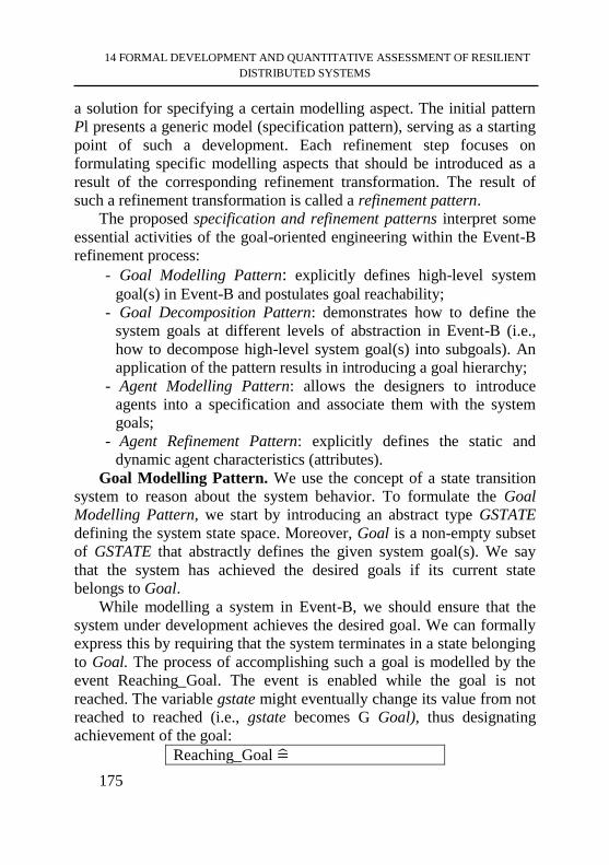
14 FORMAL DEVELOPMENT AND QUANTITATIVE ASSESSMENT OF RESILIENT

DISTRIBUTED SYSTEMS

175

a solution for specifying a certain modelling aspect. The initial pattern

Pl presents a generic model (specification pattern), serving as a starting

point of such a development. Each refinement step focuses on

formulating specific modelling aspects that should be introduced as a

result of the corresponding refinement transformation. The result of

such a refinement transformation is called a refinement pattern.

The proposed specification and refinement patterns interpret some

essential activities of the goal-oriented engineering within the Event-B

refinement process:

- Goal Modelling Pattern: explicitly defines high-level system

goal(s) in Event-B and postulates goal reachability;

- Goal Decomposition Pattern: demonstrates how to define the

system goals at different levels of abstraction in Event-B (i.e.,

how to decompose high-level system goal(s) into subgoals). An

application of the pattern results in introducing a goal hierarchy;

- Agent Modelling Pattern: allows the designers to introduce

agents into a specification and associate them with the system

goals;

- Agent Refinement Pattern: explicitly defines the static and

dynamic agent characteristics (attributes).

Goal Modelling Pattern. We use the concept of a state transition

system to reason about the system behavior. To formulate the Goal

Modelling Pattern, we start by introducing an abstract type GSTATE

defining the system state space. Moreover, Goal is a non-empty subset

of GSTATE that abstractly defines the given system goal(s). We say

that the system has achieved the desired goals if its current state

belongs to Goal.

While modelling a system in Event-B, we should ensure that the

system under development achieves the desired goal. We can formally

express this by requiring that the system terminates in a state belonging

to Goal. The process of accomplishing such a goal is modelled by the

event Reaching_Goal. The event is enabled while the goal is not

reached. The variable gstate might eventually change its value from not

reached to reached (i.e., gstate becomes G Goal), thus designating

achievement of the goal:

Reaching_Goal =̂

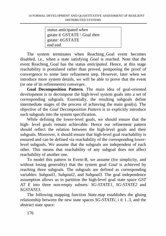
14 FORMAL DEVELOPMENT AND QUANTITATIVE ASSESSMENT OF RESILIENT

DISTRIBUTED SYSTEMS

176

status anticipated when

gstate ∈ GSTATE \ Goal then

gstate: ∈GSTATE

end end

The system terminates when Reaching_Goal event becomes

disabled, i.e., when a state satisfying Goal is reached. Note that the

event Reaching_Goal has the status anticipated. Hence, at this stage

reachability is postulated rather than proved, postponing the proof of

convergence to some later refinement step. However, later when we

introduce more system details, we will be able to prove that the event

(or one of its refinements) converges.

Goal Decomposition Pattern. The main idea of goal-oriented

development is to decompose the high-level system goals into a set of

corresponding subgoals. Essentially, the resulting subgoals define

intermediate stages of the process of achieving the main goal(s). The

objective of the Goal Decomposition Pattern is to explicitly introduce

such subgoals into the system specification.

While defining the lower-level goals, we should ensure that the

high- level goals remain achievable. Hence our refinement pattern

should reflect the relation between the high-level goals and their

subgoals. Moreover, it should ensure that high-level goal reachability is

ensured and can be defined via reachability of the corresponding lower-

level subgoals. We assume that the subgoals are independent of each

other. This means that reachability of any subgoal does not affect

reachability of another one.

To model this pattern in Event-B, we assume (for simplicity, and

without losing generality) that the system goal Goal is achieved by

reaching three subgoals. The subgoals are defined as corresponding

variables: Subgoal1, Subgoal2, and Subgoal3. The goal independence

assumption allows us to partition the high-level goal state space GST

AT E into three non-empty subsets: SG-STATE1, SG-STATE2 and

SGSTATE3.

The following mapping function State.map establishes the gluing

relationship between the new state spaces SG-STATEi, i ∈ 1..3, and the

abstract state space:

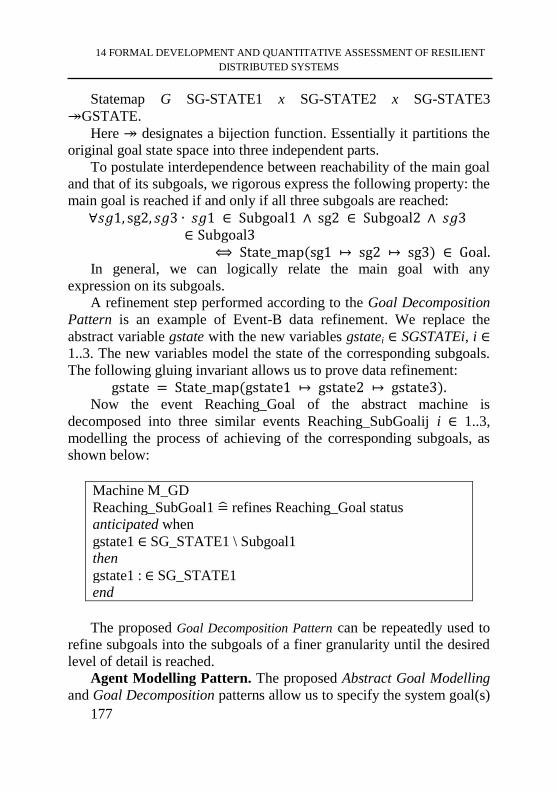
14 FORMAL DEVELOPMENT AND QUANTITATIVE ASSESSMENT OF RESILIENT

DISTRIBUTED SYSTEMS

177

Statemap G SG-STATE1 x SG-STATE2 x SG-STATE3

↠GSTATE.

Here ↠ designates a bijection function. Essentially it partitions the

original goal state space into three independent parts.

To postulate interdependence between reachability of the main goal

and that of its subgoals, we rigorous express the following property: the

main goal is reached if and only if all three subgoals are reached:

∀𝑠𝑔1, sg2, 𝑠𝑔3 ∙ 𝑠𝑔1 ∈ Subgoal1 ∧ sg2 ∈ Subgoal2 ∧ 𝑠𝑔3 ∈ Subgoal3

⟺ State_map(sg1 ↦ sg2 ↦ sg3) ∈ Goal. In general, we can logically relate the main goal with any

expression on its subgoals.

A refinement step performed according to the Goal Decomposition

Pattern is an example of Event-B data refinement. We replace the

abstract variable gstate with the new variables gstatei ∈ SGSTATEi, i ∈

1..3. The new variables model the state of the corresponding subgoals.

The following gluing invariant allows us to prove data refinement:

gstate = State_map(gstate1 ↦ gstate2 ↦ gstate3). Now the event Reaching_Goal of the abstract machine is

decomposed into three similar events Reaching_SubGoalij i ∈ 1..3,

modelling the process of achieving of the corresponding subgoals, as

shown below:

Machine M_GD

Reaching_SubGoal1 =̂ refines Reaching_Goal status

anticipated when

gstate1 ∈ SG_STATE1 \ Subgoal1

then

gstate1 : ∈ SG_STATE1

end

The proposed Goal Decomposition Pattern can be repeatedly used to

refine subgoals into the subgoals of a finer granularity until the desired

level of detail is reached.

Agent Modelling Pattern. The proposed Abstract Goal Modelling

and Goal Decomposition patterns allow us to specify the system goal(s)

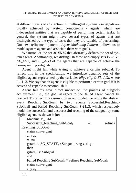
14 FORMAL DEVELOPMENT AND QUANTITATIVE ASSESSMENT OF RESILIENT

DISTRIBUTED SYSTEMS

178

at different levels of abstraction. In multi-agent systems, (sub)goals are

usually achieved by system components - agents, which are

independent entities that are capable of performing certain tasks. In

general, the system might have several types of agents that are

distinguished by the type of tasks that they are capable of performing.

Our next refinement pattern - Agent Modelling Pattern - allows us to

model system agents and associate them with goals.

We introduce the set AGENTS that abstractly defines the set of sys-

tem agents. Additionally, we distinguish three non-empty sets EL-AG1,

EL_AG2, and EL_AG3 of the agents that are capable of achieve the

corresponding subgoals.

Agent might fail while trying to achieve a certain subgoal. To

reflect this in the specification, we introduce dynamic sets of the

eligible agents represented by the variables eligi, eligi ⊆ EL_AGi, where

i ∈ 1..3. We say that an agent is eligible to perform a certain goal if it is

active and capable to accomplish it.

Agent failures have direct impact on the process of subgoals

achievement, i.e., the goal assigned to the failed agent cannot be

reached. To reflect this assumption in our model, we refine the abstract

event Reaching_SubGoali by two events SuccessfuLReaching-

SubGoali and Failed_Reaching_SubGoali, i ∈1..3, which respectively

model the successful and unsuccessful reaching of the subgoal by some

eligible agent, as shown below:

Machine M_AM

Successful_Reaching_SubGoal1 =̂ refines

Reaching_SubGoal1

status convergent

any ag

when

gstate1 ∈ SG_STATE1 \ Subgoal1 ∧ ag ∈ elig1

then

gstate1 : ∈ Subgoal1

end

Failed Reaching SubGoal1 =̂ refines Reaching SubGoal1

status convergent

any ag

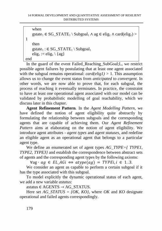
14 FORMAL DEVELOPMENT AND QUANTITATIVE ASSESSMENT OF RESILIENT

DISTRIBUTED SYSTEMS

179

when

gstate1 ∈ SG_STATE1 \ Subgoal1 ∧ ag ∈ elig1 ∧ card(elig1) >

1

then

gstate1 : ∈ SG_STATE1 \ Subgoal1

elig1 := elig1 \ {ag}

end

In the guard of the event Failed_Reaching_SubGoal;L, we restrict

possible agent failures by postulating that at least one agent associated

with the subgoal remains operational: card(elig1) > 1. This assumption

allows us to change the event status from anticipated to convergent. In

other words, we are now able to prove that, for each subgoal, the

process of reaching it eventually terminates. In practice, the constraint

to have at least one operational agent associated with our model can be

validated by probabilistic modelling of goal reachability, which we

discuss later in this chapter.

Agent Refinement Pattern. In the Agent Modelling Pattern, we

have defined the notion of agent eligibility quite abstractly by

formulating the relationship between subgoals and the corresponding

agents that are capable of achieving them. Our Agent Refinement

Pattern aims at elaborating on the notion of agent eligibility. We

introduce agent attributes - agent types and agent statuses, and redefine

an eligible agent as an operational agent that belongs to a particular

agent type.

We define an enumerated set of agent types AG_TYPE={ TYPE1,

TYPE2, TYPE3} and establish the correspondence between abstract sets

of agents and the corresponding agent types by the following axioms:

∀ag ∙ 𝑎𝑔 ∈ 𝐸𝐿_𝐴𝐺𝑖 ⟺ 𝑎𝑡𝑦𝑝𝑒(𝑎𝑔) = 𝑇𝑌𝑃𝐸𝑖, 𝑖 ∈ 1. .3. We consider an agent as capable to perform a certain subgoal if it

has the type associated with this subgoal.

To model explicitly the dynamic operational status of each agent,

we add a new variable astatus:

astatus ∈ AGENTS → AG_STATUS.

Here set AG_STATUS = {OK, KO}, where OK and KO designate

operational and failed agents correspondingly.

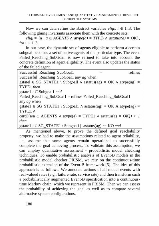
14 FORMAL DEVELOPMENT AND QUANTITATIVE ASSESSMENT OF RESILIENT

DISTRIBUTED SYSTEMS

180

Now we can data refine the abstract variables eligi, i ∈ 1..3. The

following gluing invariants associate them with the concrete sets:

eligi = {a | a ∈ AGENTS ∧ atype(a) = TYPEi ∧ astatus(a) = OK},

for i ∈ 1..3.

In our case, the dynamic set of agents eligible to perform a certain

subgoal becomes a set of active agents of the particular type. The event

Failed_Reaching_SubGoali is now refined to take into account the

concrete definition of agent eligibility. The event also updates the status

of the failed agent.

Successful_Reaching_SubGoal1 = refines

Successful_Reaching_SubGoal1 any ag when

gstatel ∈ SG_STATE1 \ Subgoall ∧ astatus(ag) = OK ∧ atype(ag) =

TYPE1 then

gstate1 : G Subgoal1 end

Failed_Reaching_SubGoal1 = refines Failed_Reaching_SubGoal1

any ag when

gstate1 ∈ SG_STATE1 \ Subgoal1 ∧ astatus(ag) = OK A atype(ag) =

TYPE1 ∧

card({a\a ∈ AGENTS ∧ atype(a) = TYPE1 ∧ astatus(a) = OK}) > 1

then

gstate1 : ∈ SG_STATE1 \ Subgoali || astatus(ag) := KO end

As mentioned above, to prove the defined goal reachability

property, we had to make the assumptions related to agent reliability,

i.e., assume that some agents remain operational to successfully

complete the goal achieving process. To validate this assumption, we

can employ quantitative assessment - probabilistic model checking

techniques. To enable probabilistic analysis of Event-B models in the

probabilistic model checker PRISM, we rely on the continuous-time

probabilistic extension of the Event-B framework [5]. The idea of this

approach is as follows. We annotate actions of all model events with

real-valued rates (e.g., failure rate, service rate) and then transform such

a probabilistically augmented Event-B specification into a continuous-

time Markov chain, which we represent in PRISM. Then we can assess

the probability of achieving the goal as well as to compare several

alternative system configurations.

14 FORMAL DEVELOPMENT AND QUANTITATIVE ASSESSMENT OF RESILIENT

DISTRIBUTED SYSTEMS

181

The resilience-explicit goal-oriented refinement approach presented

above allowed us to identify the key concepts required for formal

development of resilient MAS. It has inspired as to propose a

conceptual framework for goal-oriented reasoning about resilient MAS

that puts a specific emphasis of rigorous definition of system

reconfigurability. Next we overview the proposed formalization.

14.6 Formal Goal-Oriented Reasoning About Resilient Re-

configurable MAS

In this section let us overview proposed formalization of the

reconfigurability concept within a multi-agent goal-oriented

framework. The aim is to gradually define the notions of system goals

and agents together with their different interrelationships. Let us

systematically introduce the necessary constraints on the system

dynamics to facilitate derivation of a necessary reconfiguration

mechanism. Here we consider reconfigurability as an ability of agents

to redistribute their responsibilities and associations to ensure goal

reachability.

Goal-oriented State Transition System. We start by extending the

standard definition of a state transition system (including the set of all

system states V, the next-state relation Trans, and the set of initial

system states Init) with the notion of goals that a system is trying to

accomplish. More specifically, we introduce the set of all possible

system goals G and the function GMap mapping a given system goal to

a subset of system states:

GMap ∶ ℊ → P(Σ). Essentially, the function GMap assigns semantics to any goal from

G by associating it with a non-empty set of states (a predicate) of Σ.

Further let us extend the goal-oriented state transition system with

the notion of subgoals. To introduce inter-relationships between the

system goals, e.g., distinguishing particular goals and their subgoals,

we define two structures - the relation on goals G_graph and the

function SGMap:

G_graph : ℊ ↔ ℊ and SGMap : ℊ → P(𝛴).

Essentially, G_graph describes relationships between different

goals, e.g., how a particular goal can be decomposed into its subgoals

14 FORMAL DEVELOPMENT AND QUANTITATIVE ASSESSMENT OF RESILIENT

DISTRIBUTED SYSTEMS

182

and so on. SGMap(g) stands for mapping an arbitrary expression on

subgoals of g into a set of states, corresponding to achieving the parent

goal g. Intuitively, SGMap(g) stands for the necessary precondition for

achieving goal g.

Essentially, achieving any of subgoals must contribute to reaching

the parent goal:

∀𝑔, 𝑔′: ℊ. 𝑔′ ∈ 𝑆𝑢𝑏𝑔𝑜𝑎𝑙𝑠(𝑔) ⇒ 𝑆𝐺𝑀𝑎𝑝(𝑔) ∩ 𝐺𝑀𝑎𝑝(𝑔′) ≠ ∅, where 𝑆𝑢𝑏𝑔𝑜𝑎𝑙𝑠(𝑔) = {𝑔′ ∶ ℊ | (𝑔 ↦ 𝑔′) ∈ 𝐺_𝑔𝑟𝑎𝑝ℎ}.

Introducing Agents. Next, we extend a goal-oriented state

transition system by introducing agents that can carry out tasks required

for achieving the system goals. We introduce the type (set) A for all

possible system agents and define the function Active to distinguish a

subset of active agents in the current system state:

Active : Σ → P(A).

By “active” agents we mean the agents that can carry out the tasks

in order to achieve the system goals. In its turn, the inactive agents are

either the agents which are not currently present in the system or those

which failed and thus incapable to carry out any tasks.

To reflect the heterogeneous nature of multi-agent systems, next we

introduce possible agent attributes. Namely, we associate certain

classes of agents with specific types of system goals they are able to

accomplish. To formalize it, we first introduce classifications of system

agents and goals and then define relationships between the introduced

classes.

The following functions

𝑎𝑡𝑦𝑝𝑒 ∶ A → 𝐴𝑇𝑦𝑝𝑒 𝑎𝑛𝑑 𝑔𝑡𝑦𝑝𝑒 ∶ ℊ → 𝐺𝑇𝑦𝑝𝑒, associate each agent and goal with their respective type, where

AType and GType are abstract types containing all possible agent and

goal types respectively.

The separate goals of the same goal type can be achieved

independently, i.e., can be assigned to different agents that work in

parallel to accomplish them:

∀g1, g2 ∶ ℊ, 𝑔𝑡: 𝐺𝑇𝑦𝑝𝑒. 𝑔𝑡𝑦𝑝𝑒(𝑔1) = 𝑔𝑡 ∧ 𝑔𝑡𝑦𝑝𝑒(𝑔2) = 𝑔𝑡 ∧ g1 ≠ g2 ∧

𝐺𝑀𝑎𝑝(𝑔1) ∩ 𝐺𝑀𝑎𝑝(𝑔2) = ∅,

14 FORMAL DEVELOPMENT AND QUANTITATIVE ASSESSMENT OF RESILIENT

DISTRIBUTED SYSTEMS

183

To represent interrelationships between different agent and goal

types, we introduce the relation AG_Rel:

𝐴𝐺_𝑅𝑒𝑙: 𝐴𝑇𝑦𝑝𝑒 ↔ 𝐺𝑇𝑦𝑝𝑒. This formalizes a connection between the corresponding agent and

goal types clarifies which agents can be given the tasks related to

specific system goals.

Agent Subordination and Supervision. Defining agent types and

hierarchy of goal types allows us to introduce a subordination structure

between agent types. Essentially, subordination means that one agent

may be the “master” (manager) of the other agent(s). Naturally, agent

subordination supposes that some agents “supervise” activities of other

agents. Moreover, a supervising agent can give concrete goal

assignments to subordinate agents, which, in turn, should “report” to its

supervisors once the assigned goal has been accomplished. The

unreached system goals can be also dynamically partitioned among the

supervisor agents, essentially modelling accepted responsibilities of

those agents for supervision over some goals.

To introduce such subordination, we define a relation on agent

types, called ASub:

𝐴_𝑆𝑢𝑏 ∶ 𝐴𝑇𝑦𝑝𝑒 ↔ 𝐴𝑇𝑦𝑝𝑒. Moreover, for each pair of subordinated agent types, there should

exist (at least one) pair of the related goal types such that goals of the

parent goal type can be handled by agents of the “master” agent type,

while goals of the subgoal type can be handled by agents of the

subordinate agent type.

Let us note that the introduced notions of agent types,

subordination, ability to accomplish or supervise a particular goal,

constitute static properties of a multi-agent goal-oriented system. On

the other hand, since agents can change their active/inactive status

during system execution, the function Active expresses a dynamic

system characteristic. To formally define a system configuration and

the corresponding reconfiguration mechanism for tolerating system

changes, we need to define additional dynamic system characteristics.

First, in a specific dynamic system state, a particular agent can be

14 FORMAL DEVELOPMENT AND QUANTITATIVE ASSESSMENT OF RESILIENT

DISTRIBUTED SYSTEMS

184

attached to another agent, which serves as its supervisor. A specific

goal that has not been yet reached can be put under responsibility of a

particular supervisor agent. Moreover, a specific goal can be assigned

by a supervisor to one of its subordinate agents. Later, the assigned goal

can be executed by the corresponding agent. If the agent fails to achieve

the assigned task, its goal can be reassigned to another agent capable to

achieve it.

We formulate these dynamic notions formally. For instance, agent

attachment is defined as the function Attached, such that

- Attached : Σ → 𝑃(𝐴 𝑥 𝐴), - ∀σ ∶ Σ, 𝑎1, 𝑎2 ∶ 𝐴. (𝑎1 ↦ 𝑎2) ∈ Attached(σ) ∧ - 𝑎1 ∈ Active(σ) ∧ 𝑎2 ∈ Active(σ) ∧ atype(a1) ↦ atype(a2) ∈ ASub ∧ ¬(∃𝑎3 ∶ 𝐴. 𝑎3 ≠ 𝑎1 ∧ (𝑎3 ↦ 𝑎2) ∈ Attached(σ)).

Therefore, for any agents a1, a2 and system state σ, the expression

(a1 ↦ a2) e Attached(σ) implies that (i) both agents are active in σ, (ii)

the agent type of a2 is subordinate to that of a1, and (iii) the agent a2 is

not currently attached to any other supervisor agent.

Moreover, a goal-oriented multi-agents system supports agent

attachment if, at any point where the conditions for agent attachment

are satisfied, the system has an opportunity (but not an obligation) to do

such an action.

Similarly to agent attachment, we define goal responsibility (the

corresponding function called Responsible) and goal assignment (the

corresponding function called Assigned) as system dynamic attributes

(i.e., they depend on the current system state). Goal responsibility

specifies the relationships between certain goals and the agents

currently supervising them. In its turn, goal assignment defines the

relationships between the goals and pair of agents that supervise and

perform these goals respectively. Moreover, a goal-oriented multi-

agents system supports goal responsibility and goal assignment if, at

any point where the conditions for these properties are satisfied, the

system is able to do these actions.

Now, the introduced above notions and characteristics allow us to

define notion of a reconfigurable system and reason about system

reconfigurability.

14 FORMAL DEVELOPMENT AND QUANTITATIVE ASSESSMENT OF RESILIENT

DISTRIBUTED SYSTEMS

185

Reasoning about System Reconfiguration Towards Goal

Achievement. Based on the definitions, we can explicitly define multi-

agent systems that support system dynamic reconfiguration.

Specifically, these are the systems that allow redistributing

(unassigned) goals to different responsible agents or reattaching

(unassigned) agents to different supervisor agents. Moreover, the

following properties must hold:

∀σ ∶ Σ, g ∶ ℊ, ∶ 𝑎1, 𝑎2 ∶ 𝐴. (g ↦ 𝑎1) ∈ Responsible(σ) ∧ gtype(g)

∈ AS_goals(atype(a2)) ∧

¬(∃𝑎3 ∶ 𝐴. (g ↦ 𝑎1 ↦ 𝑎3)) ∈ Assigned(σ)) ⇒ ∃σ′ ∶ Σ. (σ ↦ σ′) ∈ Trans ∧ (g ↦ 𝑎2) ∈ Responsible(σ′) and

∀σ ∶ 𝛴, 𝑎𝑙, 𝑎2, 𝑎3 ∶ 𝐴. (al ↦ 𝑎2)

∈ 𝐴𝑡𝑡𝑎𝑐ℎ𝑒𝑑(σ) ∧ (𝑎𝑡𝑦𝑝𝑒(𝑎3) 𝑎𝑡𝑦𝑝𝑒(𝑎2))

∈ 𝐴_𝑆𝑢𝑏 ∧ ¬(∃𝑔 ∶ ℊ. (g ↦ al ↦ a2)) ∈ 𝐴𝑠𝑠𝑖𝑔𝑛𝑒𝑑(σ)) ⇒

∃σ′ ∶ 𝛴. (σ ↦ σ′) ∈ Trans ∧ (a3 ↦ 𝑎2) ∈ Attached(σ). Essentially, these two properties require the existence of state

transitions allowing to redistribute goal responsibility and agent

attachment. Here the condition gtype(g) ∈ AS_goals(atype(a2)) checks

that the type of the agent a2 allows the agent to supervise the goal g,

while the condition (atype(a3) ↦ atype(a2)) ∈ A_Sub requires that the

agent type of a2 is subordinate to that of a3.

Theorem: Goal reachability in a reconfigurable agent system.

For a reconfigurable goal-oriented multi-agent system (G, Σ, Init,

Trans, GMap, A, Active), the following property is true:

∀σ ∶ 𝛴, 𝑔 ∶ ℊ. σ ∈ dom( 𝑇𝑟𝑎𝑛𝑠) ∧ σ ∉ 𝐺𝑀𝑎𝑝(𝑔) ⇒ ∃σ′ ∶ 𝛴. (σ ↦ σ′) ∈ 𝑇𝑟𝑎𝑛𝑠 + ∧ σ′ ∈ 𝐺𝑀𝑎𝑝(𝑔).

Essentially, theorem states, that for a reconfigurable goal-oriented

multiagent system, any goal that is not yet reached at any (non-final)

system state is reachable. Let us note that the theorem is proved to

formally demonstrate that all the introduced notions and mechanisms

are sufficient to ensure goal reachability in such a system.

The goal-oriented framework provides us with a suitable basis for

reasoning about reconfigurability. It allows us to define reconfiguration

14 FORMAL DEVELOPMENT AND QUANTITATIVE ASSESSMENT OF RESILIENT

DISTRIBUTED SYSTEMS

186

as ability of agents to redistribute their responsibilities to ensure goal

reachability. The proposed formal systematization of the involved

concepts can be seen as generic guidelines for formal development of

reconfigurable systems.

14.7 Modelling and Assessment of Resilient Architectures

In this section, we focus on the problem of formal modelling and

quantitative assessment of resilient architectures. In particular, we

experiment with different architectural alternatives implementing a

well-known fault tolerant mechanism for distributed systems (WAL).

Each alternative provide the developers with different reliability

guarantees expressed in the terms of data consistency and data integrity

properties. However, since higher reliability usually results in lower

performance, it is desirable to quantitatively assess this ratio under

different configurations parameters and loads.

Let us start this section by briefly describing the WAL mechanism.

Then we demonstrate how to use the employed refinement approach to

derive resilient architectures. Finally, let us propose a graphical

notation facilitating construction and validation of models for resilience

assessment in SimPy - a library and development framework in Python.

WAL mechanism and data base replication. The WAL

mechanism is a standard data base technique for ensuring data integrity.

The main principle of WAL is to apply the requested changes to data

files only after they have been logged, i.e., recorded into a log file and

the file has been stored in a persistent storage. If the system crashes, it

can be recovered using the log file. Therefore, the WAL method

ensures fault tolerance. Moreover, the WAL mechanism helps to

optimize the system performance, since only the log file (rather than all

the data changes) should be written to the persistent storage to

guarantee that a transaction is (eventually) committed.

However, an implementation of a persistent storage, i.e., the

guaranteeing that the node containing the log file never crashes, is hard

to achieve. To ensure resilience, the proposed mechanism can be

combined with the required replication techniques as follows. In a

distributed data store consisting of a number of nodes distributed across

different physical locations, one of the nodes, called master, is

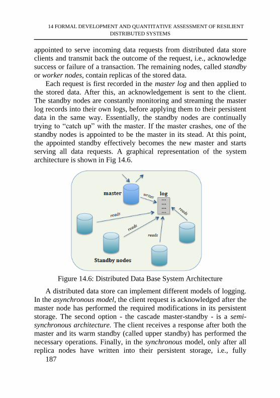
14 FORMAL DEVELOPMENT AND QUANTITATIVE ASSESSMENT OF RESILIENT

DISTRIBUTED SYSTEMS

187

appointed to serve incoming data requests from distributed data store

clients and transmit back the outcome of the request, i.e., acknowledge

success or failure of a transaction. The remaining nodes, called standby

or worker nodes, contain replicas of the stored data.

Each request is first recorded in the master log and then applied to

the stored data. After this, an acknowledgement is sent to the client.

The standby nodes are constantly monitoring and streaming the master

log records into their own logs, before applying them to their persistent

data in the same way. Essentially, the standby nodes are continually

trying to “catch up” with the master. If the master crashes, one of the

standby nodes is appointed to be the master in its stead. At this point,

the appointed standby effectively becomes the new master and starts

serving all data requests. A graphical representation of the system

architecture is shown in Fig 14.6.

Figure 14.6: Distributed Data Base System Architecture

A distributed data store can implement different models of logging.

In the asynchronous model, the client request is acknowledged after the

master node has performed the required modifications in its persistent

storage. The second option - the cascade master-standby - is a semi-

synchronous architecture. The client receives a response after both the

master and its warm standby (called upper standby) has performed the

necessary operations. Finally, in the synchronous model, only after all

replica nodes have written into their persistent storage, i.e., fully

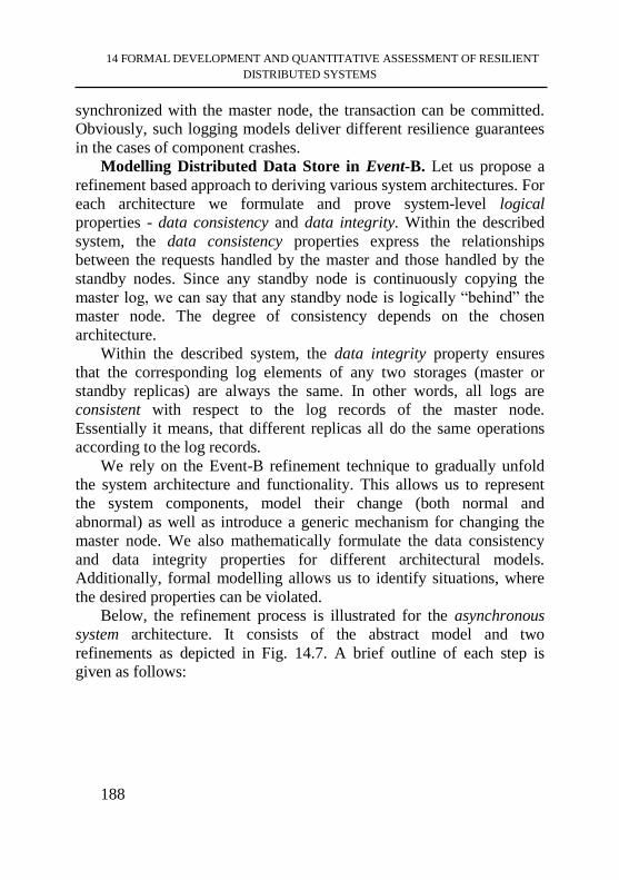
14 FORMAL DEVELOPMENT AND QUANTITATIVE ASSESSMENT OF RESILIENT

DISTRIBUTED SYSTEMS

188

synchronized with the master node, the transaction can be committed.

Obviously, such logging models deliver different resilience guarantees

in the cases of component crashes.

Modelling Distributed Data Store in Event-B. Let us propose a

refinement based approach to deriving various system architectures. For

each architecture we formulate and prove system-level logical

properties - data consistency and data integrity. Within the described

system, the data consistency properties express the relationships

between the requests handled by the master and those handled by the

standby nodes. Since any standby node is continuously copying the

master log, we can say that any standby node is logically “behind” the

master node. The degree of consistency depends on the chosen

architecture.

Within the described system, the data integrity property ensures

that the corresponding log elements of any two storages (master or

standby replicas) are always the same. In other words, all logs are

consistent with respect to the log records of the master node.

Essentially it means, that different replicas all do the same operations

according to the log records.

We rely on the Event-B refinement technique to gradually unfold

the system architecture and functionality. This allows us to represent

the system components, model their change (both normal and

abnormal) as well as introduce a generic mechanism for changing the

master node. We also mathematically formulate the data consistency

and data integrity properties for different architectural models.

Additionally, formal modelling allows us to identify situations, where

the desired properties can be violated.

Below, the refinement process is illustrated for the asynchronous

system architecture. It consists of the abstract model and two

refinements as depicted in Fig. 14.7. A brief outline of each step is

given as follows:

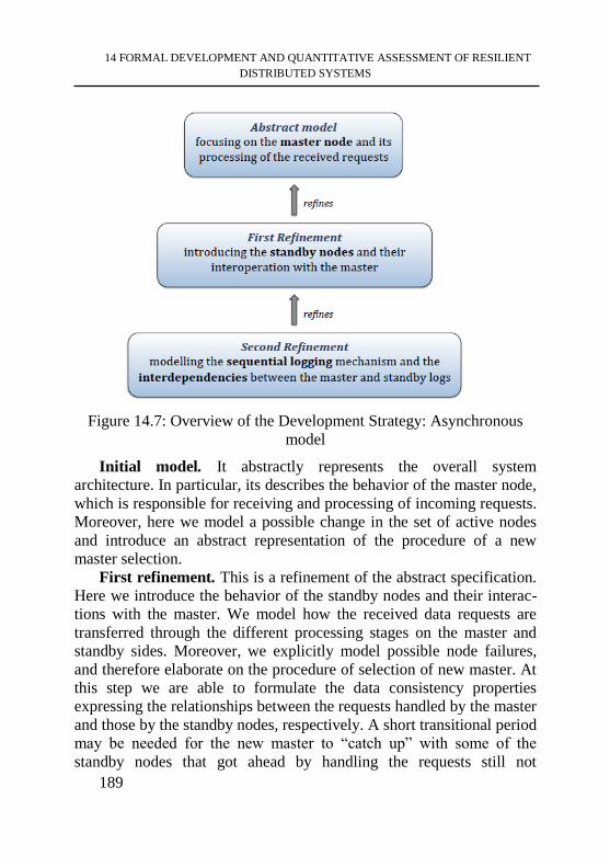
14 FORMAL DEVELOPMENT AND QUANTITATIVE ASSESSMENT OF RESILIENT

DISTRIBUTED SYSTEMS

189

Figure 14.7: Overview of the Development Strategy: Asynchronous

model

Initial model. It abstractly represents the overall system

architecture. In particular, its describes the behavior of the master node,

which is responsible for receiving and processing of incoming requests.

Moreover, here we model a possible change in the set of active nodes

and introduce an abstract representation of the procedure of a new

master selection.

First refinement. This is a refinement of the abstract specification.

Here we introduce the behavior of the standby nodes and their interac-

tions with the master. We model how the received data requests are

transferred through the different processing stages on the master and

standby sides. Moreover, we explicitly model possible node failures,

and therefore elaborate on the procedure of selection of new master. At

this step we are able to formulate the data consistency properties

expressing the relationships between the requests handled by the master

and those by the standby nodes, respectively. A short transitional period

may be needed for the new master to “catch up” with some of the

standby nodes that got ahead by handling the requests still not

14 FORMAL DEVELOPMENT AND QUANTITATIVE ASSESSMENT OF RESILIENT

DISTRIBUTED SYSTEMS

190

committed by the new master. To address this problem, we introduce an

explicit representation of the transition period and redefine the

consistency property.

Second refinement. This model explicitly introduces the sequential

logging mechanism and the resulting interdependencies between the

master and standby logs. The model is obtained as a result of a data

refinement. An introduction of the sequential representation of the

component log allows us to refine some proven invariants as well as

prove some new ones. In particular, we formulate and prove the log

data integrity properties as the following model invariants:

∀𝑐1, 𝑐2, 𝑖 ∙ 𝑐1 ∈ comp ∧ 𝑐2 ∈ comp ∧ i ∈ 1 . . index_written(cV) ∧

i ∈ 1 . . index_written(c2) ⇒ 𝑙𝑜𝑔(𝑐1)(𝑖) = 𝑙𝑜𝑔(𝑐2)(𝑖). The property states that the corresponding log elements of any two

storages are always the same.

The formal development of the semi-synchronous and synchronous

architectures is essentially repeats the refinement steps presented for the

asynchronous model. However, in the semi-synchronous case, in the

abstract model we also introduce the upper standby component and its

interoperations with the master node. In both cases, we implement

specific architectural solutions for the corresponding architecture and

respective restrictions on the component behaviors. Therefore, the data

consistency properties for each architecture are reformulated and

proved. In its turn, the data integrity property is architectural-

independent and remains the same. The resulting Event-B formal

models can be served as a starting point for future development of a

specific distributed application.

The outlined refinement process supports qualitative reasoning

about resilience. However, it is also desirable to quantitatively assess

sensitivity of the architecture to changes of its configuration

parameters. To enable such quantitative assessment of resilience

characteristics, in particular, to analyze the performance/fault tolerance

ratio of the architectural alternatives, we integrate formal modelling in

Event-B with discrete-event simulation in SimPy. Next we overview

the proposed integrated approach.

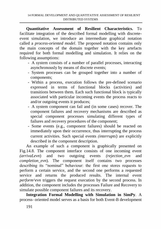
14 FORMAL DEVELOPMENT AND QUANTITATIVE ASSESSMENT OF RESILIENT

DISTRIBUTED SYSTEMS

191

Quantitative Assessment of Resilient Characteristics. To

facilitate integration of the described formal modelling with discrete-

event simulation, we introduce an intermediate graphical notation

called a process-oriented model. The proposed notation contains only

the main concepts of the domain together with the key artefacts

required for both formal modelling and simulation. It relies on the

following assumptions:

- A system consists of a number of parallel processes, interacting

asynchronously by means of discrete events;

- System processes can be grouped together into a number of

components;

- Within a process, execution follows the pre-defined scenario

expressed in terms of functional blocks (activities) and

transitions between them. Each such functional block is typically

associated with particular incoming events the process reacts to

and/or outgoing events it produces;

- A system component can fail and (in some cases) recover. The

component failures and recovery mechanisms are described as

special component processes simulating different types of

failures and recovery procedures of the component;

- Some events (e.g., component failures) should be reacted on

immediately upon their occurrence, thus interrupting the process

current activities. Such special events (interrupts) are explicitly

described in the component description.

An example of such a component is graphically presented on

Fig.14.8. The component interface consists of one incoming event

(arrivaLevn) and two outgoing events (rejection_evn and

completion_evn). The component itself contains two processes

describing its “nominal” behaviour: the first one stores requests to

perform a certain service, and the second one performs a requested

service and returns the produced results. The internal event

perform^evn triggers the request execution by the second process. In

addition, the component includes the processes Failure and Recovery to

simulate possible component failures and its recovery.

Integration Formal Modelling with Simulation in SimPy. A

process- oriented model serves as a basis for both Event-B development

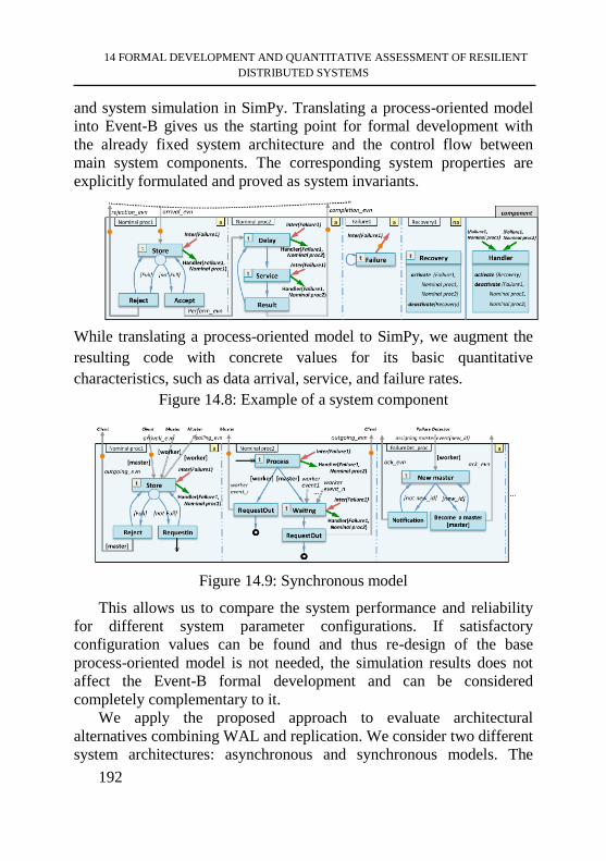
14 FORMAL DEVELOPMENT AND QUANTITATIVE ASSESSMENT OF RESILIENT

DISTRIBUTED SYSTEMS

192

and system simulation in SimPy. Translating a process-oriented model

into Event-B gives us the starting point for formal development with

the already fixed system architecture and the control flow between

main system components. The corresponding system properties are

explicitly formulated and proved as system invariants.

While translating a process-oriented model to SimPy, we augment the

resulting code with concrete values for its basic quantitative

characteristics, such as data arrival, service, and failure rates.

Figure 14.8: Example of a system component

Figure 14.9: Synchronous model

This allows us to compare the system performance and reliability

for different system parameter configurations. If satisfactory

configuration values can be found and thus re-design of the base

process-oriented model is not needed, the simulation results does not

affect the Event-B formal development and can be considered

completely complementary to it.

We apply the proposed approach to evaluate architectural

alternatives combining WAL and replication. We consider two different

system architectures: asynchronous and synchronous models. The

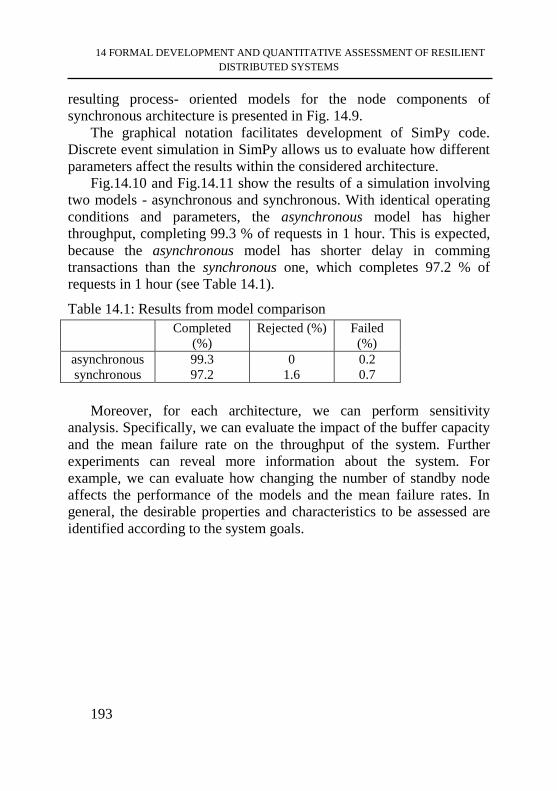
14 FORMAL DEVELOPMENT AND QUANTITATIVE ASSESSMENT OF RESILIENT

DISTRIBUTED SYSTEMS

193

resulting process- oriented models for the node components of

synchronous architecture is presented in Fig. 14.9.

The graphical notation facilitates development of SimPy code.

Discrete event simulation in SimPy allows us to evaluate how different

parameters affect the results within the considered architecture.

Fig.14.10 and Fig.14.11 show the results of a simulation involving

two models - asynchronous and synchronous. With identical operating

conditions and parameters, the asynchronous model has higher

throughput, completing 99.3 % of requests in 1 hour. This is expected,

because the asynchronous model has shorter delay in comming

transactions than the synchronous one, which completes 97.2 % of

requests in 1 hour (see Table 14.1).

Table 14.1: Results from model comparison

Completed

(%)

Rejected (%) Failed

(%)

asynchronous

synchronous

99.3

97.2

0

1.6

0.2

0.7

Moreover, for each architecture, we can perform sensitivity

analysis. Specifically, we can evaluate the impact of the buffer capacity

and the mean failure rate on the throughput of the system. Further

experiments can reveal more information about the system. For

example, we can evaluate how changing the number of standby node

affects the performance of the models and the mean failure rates. In

general, the desirable properties and characteristics to be assessed are

identified according to the system goals.

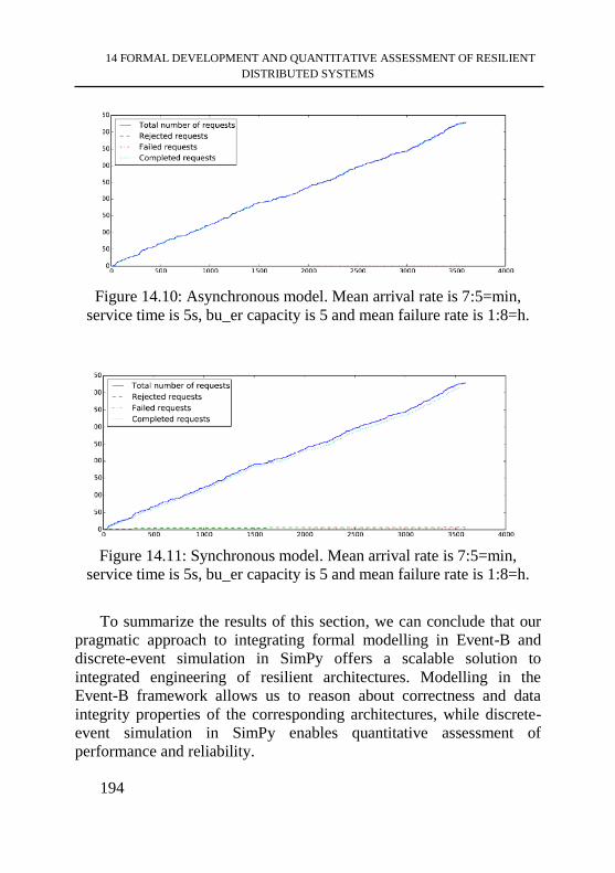
14 FORMAL DEVELOPMENT AND QUANTITATIVE ASSESSMENT OF RESILIENT

DISTRIBUTED SYSTEMS

194

Figure 14.10: Asynchronous model. Mean arrival rate is 7:5=min,

service time is 5s, bu_er capacity is 5 and mean failure rate is 1:8=h.

Figure 14.11: Synchronous model. Mean arrival rate is 7:5=min,

service time is 5s, bu_er capacity is 5 and mean failure rate is 1:8=h.

To summarize the results of this section, we can conclude that our

pragmatic approach to integrating formal modelling in Event-B and

discrete-event simulation in SimPy offers a scalable solution to

integrated engineering of resilient architectures. Modelling in the

Event-B framework allows us to reason about correctness and data

integrity properties of the corresponding architectures, while discrete-

event simulation in SimPy enables quantitative assessment of

performance and reliability.

14 FORMAL DEVELOPMENT AND QUANTITATIVE ASSESSMENT OF RESILIENT

DISTRIBUTED SYSTEMS

195

Advancement questions

1. What are principles the proposed approach relies on?

2. What is the main idea of resilience-explicit refinement process

for the systems that perform a certain predefined scenario?

3. What we should implement to model functional decomposition?

4. State the purpose of the Component Modelling and Abstract

Reconfiguration Modelling.

5. What for the multi-agent modelling paradigm is used?

6. Explain the idea of Pattern-Based Formal Development of

Resilient MAS.

7. How we can formulate the Goal Modelling Pattern?

8. What is the purpose of using Agent Modelling Pattern and Agent

Refinement Pattern

9. What is the WAL mechanism and what is the purpose of its

implementation?

10. what are main the stages of the refinement process for the

asynchronous system architecture?

REFERENCES

[1] Pereverzeva Inna Formal Development of Resilient

Distributed Systems / Inna Pereverzeva // PhD diss., Turku Centre for

Computer Science, Abo Akademi University, Faculty of Science and

Engineering, Joukahaisenkatu, Turku, Finland. – 2015.

[2] Helm R. Elements of Reusable Object-Oriented

Software/R.Helm R.EJohnson. J. Vlissides Gamma, E. Design

Patterns //Addison-Wesley Reading.-1995.

[3] Hoang T. S. Event-b patterns and their tool support /T. S.

Hoang, A. Fu¨rst, and J.-R. Abrial.// Software and System Modeling/-

2013.-12(2).-229–244,

[4] Iliasov A. Patterns for refinement automation/A. Iliasov, E.

Troubitsyna, L. Laibinis, and A. Romanovsky.// In Formal Methods for

Components and Objects - 8th International Symposium : Springer.-

2010.-pages 70–88

14 FORMAL DEVELOPMENT AND QUANTITATIVE ASSESSMENT OF RESILIENT

DISTRIBUTED SYSTEMS

196

[5] Tarasyuk A. Integrating stochastic reasoning into event-b

development./A. Tarasyuk, E. Troubitsyna, and L. Laibinis //Formal

Asp. Comput.-2015.-27(1).-53– 77

V. Sklyar, O. Illiashenko, V. Kharchenko, N. Zagorodna, R. Kozak, O. Vambol, S. Lysenko, D. Medzatyi, O. Pomorova

SECURE AND RESILIENT COMPUTING FOR INDUSTRY AND HUMAN DOMAINS.

Fundamentals of security

and resilient computing

Multi-book, Volume 1

Editor Vyacheslav Kharchenko

National Aerospace University n. a. N. E. Zhukovsky

“Kharkiv Aviation Institute” 17 Chkalova street, Kharkiv, 61070, Ukraine

http://www.khai.edu