document 707-14 frequency management group spectrum ......target spectrum utilization, operational...

Frequency Management Group

Document 707-14

SPECTRUM MANAGEMENT METRICS STANDARDS

DISTRIBUTION A: APPROVED FOR PUBLIC RELEASE DISTRIBUTION IS UNLIMITED.

ABERDEEN TEST CENTER DUGWAY PROVING GROUND

REAGAN TEST SITE WHITE SANDS MISSILE RANGE

YUMA PROVING GROUND

NAVAL AIR WARFARE CENTER AIRCRAFT DIVISION NAVAL AIR WARFARE CENTER WEAPONS DIVISION

NAVAL UNDERSEA WARFARE CENTER DIVISION, KEYPORT NAVAL UNDERSEA WARFARE CENTER DIVISION, NEWPORT

PACIFIC MISSILE RANGE FACILITY

30TH SPACE WING 45TH SPACE WING 96TH TEST WING

412TH TEST WING ARNOLD ENGINEERING DEVELOPMENT COMPLEX

NATIONAL AERONAUTICS AND SPACE ADMINISTRATION

This page intentionally left blank.

Document 707-14

Spectrum Management Metrics Standards

April 2014

Prepared by

Frequency Management Group

Range Commanders Council

Published by

Secretariat Range Commanders Council

US Army White Sands Missile Range New Mexico 88002-5110

Spectrum Management Metrics Standards RCC Document 707-14 April 2014

iii

Table of Contents Preface ........................................................................................................................................... ix

Acronyms ...................................................................................................................................... xi Chapter 1. Background and Key Concepts ........................................................................ 1-1

1.1 Introduction ...................................................................................................................... 1-1 1.2 Background ...................................................................................................................... 1-1 1.3 Scope and Purpose ........................................................................................................... 1-1 1.4 Spectrum Review ............................................................................................................. 1-2

1.4.1 Bands.................................................................................................................... 1-2 1.4.2 Time vs. Frequency Grids .................................................................................... 1-2

1.5 “Use” as “Denial to Others” ............................................................................................ 1-3 1.6 Fragmentation .................................................................................................................. 1-4 1.7 Reuse ................................................................................................................................ 1-5 1.8 Data Hierarchy ................................................................................................................. 1-5 1.9 Time Considerations ........................................................................................................ 1-6

1.9.1 Partial Assignments ............................................................................................. 1-6

1.10 Algorithm Notes............................................................................................................... 1-6

Chapter 2. Utilization Metrics (Fixed-Tile Methods) ........................................................ 2-1

2.1 Overview .......................................................................................................................... 2-1

2.1.1 Fixed-Tile Method Algorithms ............................................................................ 2-1 2.1.2 Assumptions ......................................................................................................... 2-1

2.2 Ad Hoc Mission Availability ........................................................................................... 2-2

2.2.1 Predetermined Inputs to the Algorithm................................................................ 2-2 2.2.2 Algorithm ............................................................................................................. 2-2 2.2.3 Example ............................................................................................................... 2-3

2.3 Typical Missions .............................................................................................................. 2-3

2.3.1 User-Defined Typical Missions ........................................................................... 2-3 2.3.2 Statistically Derived Typical Missions ................................................................ 2-3

2.4 Average Typical Mission Availability ............................................................................. 2-4


2.5 Spectrum Utilization ........................................................................................................ 2-5


2.6 Average Spectrum Utilization.......................................................................................... 2-5


iv

2.6.1 Predetermined Inputs to the Algorithm................................................................ 2-6 2.6.2 Algorithm ............................................................................................................. 2-6 2.6.3 Average Monthly Utilization over Several Months ............................................. 2-6 2.6.4 Average Yearly Utilization over Several Years................................................... 2-6

2.7 3D Average Spectrum Utilization Chart .......................................................................... 2-6

2.7.1 Predetermined Inputs to the Algorithm................................................................ 2-6 2.7.2 Data Structures Required ..................................................................................... 2-6 2.7.3 Algorithm Outline ................................................................................................ 2-7 2.7.4 Main Algorithm ................................................................................................... 2-7 2.7.5 Subalgorithm for Step 1c. .................................................................................... 2-8 2.7.6 Subalgorithm for Step 1d ..................................................................................... 2-8 2.7.7 Example ............................................................................................................... 2-9

2.8 2-Dimensional Spectrum Utilization Projections .......................................................... 2-12

2.8.1 Average 2-Dimensional Spectrum Utilization Time Projection ........................ 2-12 2.8.2 Average 2-Dimensional Spectrum Utilization Frequency Projection ............... 2-12 2.8.3 Maximum 2-Dimensional Spectrum Utilization Time Projection ..................... 2-13 2.8.4 Maximum 2-Dimensional Spectrum Utilization Frequency Projection ............ 2-13 2.8.5 Examples ............................................................................................................ 2-13

Chapter 3. Spectrum Reuse .................................................................................................. 3-1

3.1 Operational Interference .................................................................................................. 3-1

3.1.1 The Friis Transmission Equation ......................................................................... 3-1 3.1.2 Line of Sight ........................................................................................................ 3-3 3.1.3 Closest-Point Analysis ......................................................................................... 3-3 3.1.4 Mobile and Stationary .......................................................................................... 3-3 3.1.5 Determining Operational Interference ................................................................. 3-4

3.2 Area of Mutual Use .......................................................................................................... 3-5 3.3 Definition of Spectrum Reuse .......................................................................................... 3-5

Chapter 4. Spectral Occupancy Metrics (Area Methods) ................................................. 4-1

4.1 Overview .......................................................................................................................... 4-1

4.1.1 Counting Cells ..................................................................................................... 4-1 4.1.2 Assumptions ......................................................................................................... 4-1

4.2 Percent Occupancy with Reuse ........................................................................................ 4-1


4.3 Average POWR ............................................................................................................... 4-2

4.3.1 Predetermined Inputs to the Algorithm................................................................ 4-2 4.3.2 Algorithm ............................................................................................................. 4-2 4.3.3 Average Monthly POWR over Several Months .................................................. 4-2 4.3.4 Average Yearly POWR over Several Years ........................................................ 4-3


v

4.4 3D Average POWR Chart ................................................................................................ 4-3

4.4.1 Predetermined Inputs to the Algorithm................................................................ 4-3 4.4.2 Data Structures Required ..................................................................................... 4-3 4.4.3 Algorithm ............................................................................................................. 4-3 4.4.4 Example ............................................................................................................... 4-4

4.5 Percent Occupancy........................................................................................................... 4-4


4.6 Average Percent Occupancy ............................................................................................ 4-5

4.6.1 Predetermined Inputs to the Algorithm................................................................ 4-6 4.6.2 Algorithm ............................................................................................................. 4-6 4.6.3 Average Monthly PO over Several Months ......................................................... 4-6 4.6.4 Average Yearly PO over Several Years ............................................................... 4-6

4.7 3D Average PO ................................................................................................................ 4-6


4.8 Percent Multiple Use........................................................................................................ 4-8


4.9 Frequency Reuse Ratio .................................................................................................. 4-10

4.9.1 Derivation of FRR.............................................................................................. 4-10 4.9.2 Example ............................................................................................................. 4-10

Chapter 5. Efficiency Metrics .............................................................................................. 5-1

5.1 Scheduled Bandwidth vs. Necessary Bandwidth ............................................................. 5-1

5.1.1 Necessary or 99 Percent Power Bandwidth ......................................................... 5-1 5.1.2 Scheduled Bandwidth .......................................................................................... 5-2

5.2 Mission Modulation Efficiency ....................................................................................... 5-2 5.3 Average Mission Modulation Efficiency ......................................................................... 5-2

5.3.1 Predetermined Inputs to the Algorithm................................................................ 5-2 5.3.2 Algorithm ............................................................................................................. 5-2

5.4 Modulation Method Ratio ................................................................................................ 5-2 5.5 Mission Spectrum Efficiency ........................................................................................... 5-3 5.6 Average Mission Spectrum Efficiency ............................................................................ 5-3


vi


5.7 Average Spectrum Band Efficiency ................................................................................. 5-3


5.8 Bits Sent ........................................................................................................................... 5-4


5.9 Bits Sent per MH ............................................................................................................. 5-4


Chapter 6. Metrics By Mission Groupings ......................................................................... 6-5

6.1 Operation Size .................................................................................................................. 6-5


6.2 Operational Statistics ....................................................................................................... 6-5

Chapter 7. Scheduling Operational Metrics ....................................................................... 7-1

7.1 Requests Authorized ........................................................................................................ 7-1

7.1.1 Spectrum Request ................................................................................................ 7-1 7.1.2 Approval Categories ............................................................................................ 7-1

7.2 Assignment Canceled, Delayed, or Rescheduled ............................................................ 7-1

7.2.1 Categories ............................................................................................................ 7-2 7.2.2 Reasons ................................................................................................................ 7-2

7.3 Assignment and Operation Statistics ............................................................................... 7-2

Chapter 8. Predictive, What If, Metrics .............................................................................. 8-1

8.1 Spectrum Movement Analysis ......................................................................................... 8-1

8.1.1 Additive Method .................................................................................................. 8-1 8.1.2 3D Additive Method ............................................................................................ 8-3 8.1.3 Days Not Schedulable Method ............................................................................ 8-4 8.1.4 Method Comparison............................................................................................. 8-6

8.2 New Program Impact Analysis ........................................................................................ 8-6

Chapter 9. Spectrum Management Cost Model ................................................................. 9-1

Chapter 10. Standard Chart Layouts.................................................................................. 10-1

Appendix A. Tutorial on Interference and Spectrum Reuse ............................................. A-1

Appendix B. Glossary ............................................................................................................ B-1

Appendix C. References ........................................................................................................ C-1


vii

List of Figures Figure 1-1. Standard Time vs. Frequency Grid ...................................................................... 1-3 Figure 1-2. Fragmentation in a Time vs. Frequency Grid ...................................................... 1-4 Figure 1-3. Example Reuse..................................................................................................... 1-5 Figure 2-1. 3D Chart of Table 2-4 ........................................................................................ 2-12 Figure 2-2. Example 3D Spectrum Utilization Chart ........................................................... 2-14 Figure 2-3. Average Spectrum Utilization vs. Time Projection ........................................... 2-14 Figure 2-4. Average Spectrum Utilization vs. Frequency Projection ................................... 2-15 Figure 2-5. Maximum Spectrum Utilization vs. Time Projection ........................................ 2-15 Figure 2-6. Maximum Spectrum Utilization vs. Frequency Projection................................ 2-16 Figure 4-1. 3D Percent Occupancy with Reuse Chart for Figure 1-3 .................................... 4-4 Figure 4-2. 3D PO Chart for Figure 1-3 ................................................................................. 4-8 Figure 8-1. Spectrum Utilization before Move Analysis........................................................ 8-4 Figure 8-2. Predicted Utilization after Move Analysis ........................................................... 8-4 Figure A-1. Basic Interference ............................................................................................... A-2 Figure A-2. Basic Non-Interference and Reuse ...................................................................... A-2 Figure A-3. Closest Point in Assigned Air Space .................................................................. A-4 Figure A-4. Area of Use ......................................................................................................... A-5 Figure A-5. Seven Areas of Use, Two Areas of Mutual Use, and Associated Connected

Subgraphs ............................................................................................................ A-6

List of Tables Table 1-1. Example Scheduled Mission Profiles .................................................................. 1-3 Table 2-1. Grid of Raw and Average Availability Values (Steps 1 and 2) ........................... 2-9 Table 2-2. Empty Grid Availability Counts (Step 3) .......................................................... 2-10 Table 2-3. Grid of Availability Percentages (Step 4) .......................................................... 2-10 Table 2-4. Utilization Grid (Step 5) .................................................................................... 2-11


viii



ix

PREFACE This document presents the results of Task FM-037, “Spectrum Management Metrics

Standard assigned to the Frequency Management Group (FMG) of the Range Commanders Council (RCC). The goal of this task was to establish a standard that defines spectrum utilization, and in so doing define standard algorithms, metrics and their associated names, and some standard methods of displaying the resulting data. These algorithms and associated metrics target spectrum utilization, operational costs associated with scheduling spectrum, cost impact to projects from lack of spectrum, and other aspects of managing the radio frequency (RF) spectrum. The purpose of the task was to provide tools to answer the following questions:

1. How much spectrum is being used? 2. What is the cost of managing spectrum? 3. What is the impact of spectrum limitations on projects and the war fighter?

These standards do not necessarily define the existing capability of any test range, but

constitute a guide for the orderly implementation of common analysis tools for both ranges and range users. The usefulness of these analysis methods is highly user-dependent. Some methods will be more useful than others to individual ranges. Further, some customization is provided for and individual ranges should customize where appropriate.

Please direct any questions to:

Secretariat, Range Commanders Council ATTN: TEDT-WS-RCC 1510 Headquarters Avenue White Sands Missile Range, New Mexico 88002-5110 Telephone: (575) 678-1107, DSN 258-1107 E-mail: [email protected]

mailto:[email protected]


x



xi

ACRONYMS ∆B delta bandwidth ∆T delta time AHMA ad hoc mission availability AMME average mission modulation efficiency AMSE average mission spectrum efficiency AMU area of mutual use ASBE average spectrum band efficiency ATMA average typical mission availability bps bits per second dB decibel ERP effective radiated power FRR frequency reuse ratio FTS flight termination system IFDS Integrated Frequency Deconfliction System IRIG Interrange Instrumentation Group kHz kilohertz Mbps megabits per second MDS minimal detectable signal MME mission modulation efficiency MH megahertz hours MHz megahertz MSE mission spectrum efficiency PCM/FM pulse code modulation/frequency modulation PMU percent multiple use PO percent occupancy POWR percent occupancy with reuse RCC Range Commanders Council RF radio frequency SOQPSK shaped offset quadrature phase shift keying T&E test and evaluation TM telemetry


xii



1-1

CHAPTER 1

Background and Key Concepts

1.1 Introduction

The Spectrum Management Metrics Standards document addresses some metrics used historically by the RCC member ranges but concentrates on new metrics that have not previously been defined. This chapter provides a general background and several key concepts. The chapters following are devoted to particular types of metrics. Some of these chapters are progressive in that higher-level metrics are developed based on lower-level metrics.

1.2 Background

Until the 1980s, there was essentially enough RF spectrum to meet test and evaluation (T&E) telemetry (TM) requirements. The 1990s saw an exponential growth in these requirements as well as a decrease in available spectrum due to government selling of frequencies. This has led to difficulties in scheduling frequency assignments and, in some cases, to not being able to support all requested assignments.

Although frequency managers have recognized that this spectrum crunch has been getting worse, it has become obvious that there are neither adequate metrics nor agreed-upon methods for displaying data even if they exist. These shortcomings need to be overcome as we continue to justify Department of Defense spectrum needs to both Congress and the World Radio Conference.

The implementation of the Integrated Frequency Deconfliction System (IFDS)1 was a significant step forward in aiding frequency scheduling. Although IFDS is not a scheduling system per se, it aids deconfliction across multiple ranges, each of which has its own scheduling system. Within the context of this document, although there are other potential sources of data, IFDS has become the de facto repository for scheduled frequency assignments. Thus there is at least some data available to be analyzed. Yet it remains to define how to do the analysis and to identify additional types of data to be collected.

1.3 Scope and Purpose

This document defines standard algorithms, metrics and their associated names, and some standard methods of displaying the resulting data. These algorithms and associated metrics target spectrum utilization, operational costs associated with scheduling spectrum, cost impact to projects from lack of spectrum, and other aspects of managing TM spectrum. In other words, the purpose of this document is to provide tools to address these types of questions:

1. How much spectrum is being used and is it being used efficiently? 2. What are the quantifiable characteristics of both the test operations and the spectrum

management operation itself?

1 Range Commanders Council. Frequency Management Standard Operating Procedure for Frequency Deconfliction. RCC 706-02. March 2003. May be superseded by update. Available at http://www.wsmr.army.mil/RCCsite/Pages/Publications.aspx.

http://www.wsmr.army.mil/RCCsite/Pages/Publications.aspx


1-2

3. What is the cost of managing spectrum? 4. What is the impact of spectrum limitations on projects and the warfighter? 5. Are there methods of predicting the ability to meet future demands in the context of

changing spectrum availability and demand? 6. Are there useful historical trends that can be quantified?

This document does not describe TM instrumentation (transmitters and receivers), TM

RF standards, or frequency modulation standards. These topics are described in Interrange Instrumentation Group (IRIG) Standard 106-13.2 Further, this document does not address methods of collecting data needed to use these metrics. In particular, even though this document is generated by the Frequency Management Group, not all data, especially some costs, are generated or accessible to frequency managers.

1.4 Spectrum Review

This section reviews two relevant aspects of spectrum.

1.4.1 Bands Frequency bands are contiguous sets of frequencies. Frequency bands are the primary

unit for allocation of use. Many bands have informal names (informal means that they are sometimes in dispute). Bands available for use by the T&E community have been changing some over the last decade or so and probably will continue to change. An example is what is often referred to as the S-Band, which regulatory changes narrowed from 2200-2300 megahertz (MHz) to 2200-2290 MHz. Bands and associated informal names have been defined in IFDS and in IRIG Standard 106-13; although the bands defined in those two references are not identical.

The metrics in this document may be applied to any band and different users may find it useful to tailor the band for specific analysis.

1.4.2 Time vs. Frequency Grids As illustrated in Figure 1-1, the fundamental visualization tool for all of the spectrum

utilization analyses is a time-frequency grid with time on the x-axis and frequency on the y-axis. Four missions, listed in Table 1-1, are illustrated in the figure. Using this 2D tool, spectrum utilization can be thought of as area on the grid. In the simplest case, a single mission (frequency assignment) is a rectangle on the grid and the area of that rectangle is the mission occupancy. Many of the metrics defined are variations on the use of area.

2 Range Commanders Council. Telemetry Standards. IRIG Standard 106-13. June 2013. May be superseded by update. Available at http://www.wsmr.army.mil/RCCsite/Documents/106-13_Telemetry_Standards/.

http://www.wsmr.army.mil/RCCsite/Documents/106-13_Telemetry_Standards/


1-3

Figure 1-1. Standard Time vs. Frequency Grid

Table 1-1. Example Scheduled Mission Profiles Start Time Center Frequency

(Megahertz) Duration (Hours)

Bandwidth (Megahertz)

Mission Occupancy (Megahertz Hours)

2:00 2240 2 50 100 6:00 2230 7 10 70 7:00 2267.5 3 35 105 9:00 2242.5 5 5 25

In this example (and all examples in this standard), the y-axis is divided into 5-MHz

segments and the x-axis is divided into 1-hour increments, so that each cell in the chart is 5 MHz hours (MH).

1.5 “Use” as “Denial to Others”

When considering the use of spectrum, it is natural to think of electromagnetic signals being propagated through a particular point in space at a particular time; however, from a practical and legal point of view this is not always the case. When an assignment is scheduled by someone authorized to make that assignment, that spectrum cannot legally be used by someone else whether the project with the assignment uses it or not. Thus, if there are operational problems that delay that project from implementing its mission on time, there is some spectrum that has been used even though no signal was actually being propagated.

2200220522102215222022252230223522402245 Scheduled Mission225022552260226522702275228022852290

0:00

1:00

2:00

3:00

4:00

5:00

6:00

7:00

8:00

9:00

10:0

0

11:0

0

12:0

0

13:0

0Time (Hours)

Freq

uenc

y (M

Hz)

X

Y


1-4

More generally, spectrum is sometimes not in actual use due to buffering in time, frequency, or geography (space). All of these are fundamentally used to reduce interference. Perhaps extreme examples of this are international treaties that require certain frequencies not be used within so many miles of a national border. There are many other examples of such buffering.

Ultimately, these forms of buffering can be considered as scheduled (or assigned) forms of use without actual propagation. Whether these types of uses are captured in analyses using the metrics in this standard are dependent on how the data is recorded; however, considering “use” as “denial to others” validates the use of scheduled rather than actual spectrum use for utilization analyses.

1.6 Fragmentation

From a geometric point of view, an assignment is a rectangle in the time-frequency grid. When placing many rectangles in a grid, there are often small segments of the grid that are not covered by the rectangles. If, when attempting to place another rectangle in the grid, none of the segments are large enough to accommodate that rectangle, then the grid is considered to be fragmented. This is essentially the same as disk fragmentation on a computer. This is a somewhat subtle version of “use” as “denial to others”.

An example of when a new mission cannot be scheduled is shown in Figure 1-2. The new mission has a profile of (11 hours, 2 MHz). There is no position in the grid that such a profile does not interfere with another mission. This new mission could be scheduled if the other missions are re-scheduled, but this might not be possible due to myriad reasons.

Figure 1-2. Fragmentation in a Time vs. Frequency Grid

2200220522102215222022252230223522402245 Existing Missions22502255 Potential New Mission2260226522702275228022852290

0:00

1:00

2:00

3:00

4:00

5:00

6:00

7:00

8:00

9:00

10:0

0

11:0

0

12:0

0

13:0

0

Time (Hours)

Freq

uenc

y (M

Hz)

X

Y


1-5

Scheduling spectrum is a fundamentally difficult problem (technically it is NP-hard). Adding many of the practical constraints that exist in the real world makes this even more difficult so that fragmentation is unavoidable. Thus, the metrics provided in this standard attempt to capture the affect of fragmentation on spectrum utilization.

1.7 Reuse

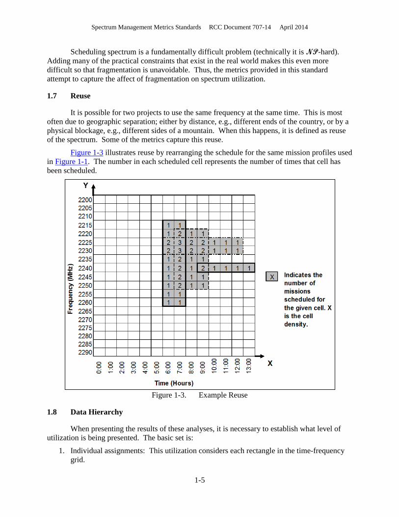
It is possible for two projects to use the same frequency at the same time. This is most often due to geographic separation; either by distance, e.g., different ends of the country, or by a physical blockage, e.g., different sides of a mountain. When this happens, it is defined as reuse of the spectrum. Some of the metrics capture this reuse.

Figure 1-3 illustrates reuse by rearranging the schedule for the same mission profiles used in Figure 1-1. The number in each scheduled cell represents the number of times that cell has been scheduled.

Figure 1-3. Example Reuse

1.8 Data Hierarchy

When presenting the results of these analyses, it is necessary to establish what level of utilization is being presented. The basic set is:

1. Individual assignments: This utilization considers each rectangle in the time-frequency grid.


1-6

2. Operations: A single test operation may include multiple assignments, either from multiple vehicles or multiple assignments per vehicle.

3. Single range: This considers the utilization across an entire range, such as Edwards Air Force Base.

4. Multiple ranges: It is reasonable to want to analyze several bases together if they share a common space; or it may be desirable to analyze all ranges.

Cross-cutting this hierarchy is the issue of frequency band(s). Most of the metrics

assume a contiguous set of frequencies - a band. For example, availability and utilization metrics are for a single band; however, higher-level analyses (e.g., for operations) might involve multiple bands.

1.9 Time Considerations

When presenting the results of these analyses, it is necessary to establish the time frame over which the analysis is being done. These standard time frames are established:

1. Work day: 0600-1800 2. Work night: 1800-0600 3. Work week: Monday through Friday

Additionally, analyses may look over particular months or years and individual users may

tailor time structures to their individual analysis needs.

1.9.1 Partial Assignments When analyzing utilization for part of a day (e.g., a work day as defined above) it is

important to include assignments that are only partially scheduled during that part of the day. Scheduling systems (such as IFDS) are likely to record assignment schedules based on start time and duration. Thus, it may be necessary to include data from outside the desired part of the day in order to obtain these partial assignments. An initial pass through the data may be required to identify these partial assignments prior to implementing the algorithms below.

1.10 Algorithm Notes

Although some metrics are described algebraically, many of the metrics are defined algorithmically. The following are standard conventions used in these algorithms.

Algorithms are described using pseudocode. For more complex cases, a high-level outline of the algorithm is provided and the detailed description is broken into a main algorithm and supportive subalgorithms.

As described below, many of the algorithms employ a stepping process through the time-frequency grid. The smallest time increment for a given scheduling system is referenced as delta time (∆T). Similarly, the smallest bandwidth increment is referenced as delta bandwidth (∆B). For IFDS, ∆T = 15 minutes and ∆B = 500 kilohertz (kHz). In the examples, ∆T =1 hour and ∆B = 5 MHz. The algorithms use the phrase “step ∆T” to indicate incrementing the reference index by ∆T.


1-7

A fundamental decision that is made in many of these algorithms is whether or not a given mission profile can be scheduled at a particular start time and center frequency. Geometrically, this is equivalent to asking if the rectangle under consideration intersects other (already scheduled) rectangles. If it does, then the mission cannot be scheduled. A specific method for determining this is not given. The algorithms simply reference “if schedulable (start time, frequency)”.

Comments in algorithms are prefixed by “//”.


1-8



2-1

CHAPTER 2

Utilization Metrics (Fixed-Tile Methods)

2.1 Overview

Spectrum utilization will be defined in terms of spectrum availability. Thus availability is defined first. Given a spectrum requirement, the portion of the spectrum that could possibly support that requirement is the portion of the spectrum that is available to it. This is based on “use” as “denial to others” and, in particular, availability metrics capture fragmentation. In general, the fundamental questions availability metrics answer are:

1. Can a mission be scheduled? 2. What is the probability of scheduling a mission?

2.1.1 Fixed-Tile Method Algorithms General definitions of each metric are provided; additionally, mathematically precise

definitions for many of the metrics are given algorithmically. Because of the discrete nature of the time-frequency grid being used, it is easy to describe methods that step through this grid with appropriate mission profiles (fixed tiles) to determine a given metric. This step-through normally determines a count of schedulable positions, which is then translated into the metric by simple equations.

The basic step-through process starts with a given mission profile (rectangle). This rectangle is then placed in the lower left-hand corner of the time-frequency grid. The question is asked: Can this mission profile be scheduled at this position? Geometrically, this is equivalent to asking if the rectangle under consideration intersects other (already scheduled) rectangles. If it does, then the mission cannot be scheduled. The rectangle is then moved up one notch (along the frequency or time axis or, iteratively, both axes). The question of schedulability is then asked again. This process is repeated until all possible positions for the rectangle have been tried. At each position, the ability to schedule or not is recorded. These schedulability counts form the basis of many of the metrics.

2.1.2 Assumptions Fundamental assumptions used in defining availability metrics are:

1. Starting times are available in discrete increments (∆T); 2. Bandwidths are available in discrete increments (∆B).

It would be possible to consider these metrics as ∆T and ∆B approach 0; however, the

current systems do not provide that level of detail and, in general, that level of analysis probably does not provide enough additional information to warrant the effort.


2-2

2.2 Ad Hoc Mission Availability

Ad hoc mission availability (AHMA) is the probability of scheduling a mission given a mission profile and flexibility in both frequency and start time. A supporting metric is an absolute count of the available (start time, frequency) pairs at which the mission can be scheduled.

Numeric interpretations:

1. AHMA > 0 means the mission can be scheduled for some (start time, frequency) pair. 2. AHMA = 1 means there are no missions scheduled in the frequency and start time ranges. 3. The greater the AHMA is, the more flexibility there is to schedule the mission. 4. 0 ≤ AHMA ≤ 1

Calculations of AHMA shall use methods mathematically equivalent to the following algorithm.

2.2.1 Predetermined Inputs to the Algorithm 1. Mission profile, including required duration and bandwidth 2. Available frequency range as minimum frequency and maximum frequency 3. Available mission time range as earliest start time and latest end time 4. Existing scheduled missions 5. Delta time 6. Delta bandwidth

2.2.2 Algorithm // Calculate times and frequencies latest start time = latest end time − required duration lowest center frequency = minimum frequency + (bandwidth / 2) highest center frequency = maximum frequency − (bandwidth / 2) // Loop through all possible schedulable positions. available count = 0 for start time = earliest start time to latest start time step ∆T

for frequency = lowest center frequency to highest center frequency step ∆B if schedulable(start time, frequency) then

available count = available count + 1 end if

end for end for // Calculate final values


2-3

number of available start times = ((latest start time − earliest start time) / ∆T) + 1 number of available frequencies = ((highest frequency − lowest frequency) / ∆B) +1 Number of (start time, frequency) pairs = number of available start times * number of available frequencies AHMA = available count / number of (start time, frequency) pairs

2.2.3 Example Given these inputs to the algorithm

1. Mission Profile: (5 hours, 15 MHz) 2. Available frequency range: 2200 - 2295 MHz 3. Available mission time range: 0000 - 1400 4. Existing scheduled missions: (See Table 1-1) 5. ∆T = 1 hour 6. ∆B = 5 MHz

Earliest start time = 0000 Latest start time = 0900 Lowest center frequency = 2207.5 Highest center frequency = 2287.5 Number of available start times = 10 Number of available frequencies = 17 Number of available (start time, frequency) pairs = 170 Available Count = 35 (10 times at 2200 MHz, 1 time at 2235 MHz, 6 times at 2205 MHz, 6 times at 2210 MHz, and 3 times each at 2265, 2270, 2275, and 2280 MHz) AHMA = 35/170 = 0.21 (or 21%)

2.3 Typical Missions

The utilization metric requires establishing typical mission profiles. This allows utilization to be representative of missions typically used at given locations. Typical missions can also be used for predictive analysis. There are two approaches to defining typical missions: user-defined and statistically derived.

A set of typical missions is defined via (duration, bandwidth) pairs, },...,1:),{( nibd ii = .

2.3.1 User-Defined Typical Missions When using user-defined typical missions, the user shall define 2-5 (duration, bandwidth)

pairs.

2.3.2 Statistically Derived Typical Missions Statistically derived typical missions shall be derived as follows. The set of missions to

be analyzed for utilization are sorted by MH. If there are less than 100 missions, then 2 bins are created. If there are more than 100 missions, then 4 bins are created. The center mission


2-4

rounding down in each of the bins (as sorted) is chosen as a typical mission. In other words for 4 bins, the 1/8, 3/8, 5/8, and 7/8 missions are chosen.

For example, if there are 1005 missions, then the 1/8 mission is mission number 125, and the 3/8, 5/8, 7/8 missions are mission numbers 376, 628, and 879 respectively.

2.4 Average Typical Mission Availability

Average typical mission availability (ATMA) is the average of AHMA for several typical mission profiles. This is a summary statistic that would give a one number estimate of the probability of scheduling a typical mission on an ad hoc basis.


1. Low ATMA (near 0) means a very low probability of scheduling an ad hoc mission. It also indicates a schedule that is very full or very fragmented. In other words, scheduling a mission would require major rework of existing scheduled missions.

2. High ATMA (near 1) means high probability of scheduling an ad hoc mission. 3. The greater the ATMA is, the more flexibility there is to schedule a mission. 4. 0 ≤ ATMA ≤ 1

The ATMA shall be calculated using methods mathematically equivalent to the following algorithm.

2.4.1 Predetermined Inputs to the Algorithm 1. Predefined typical mission profiles },...,1:),{( nibd ii = 2. Available frequency range 3. Available mission time range 4. Existing scheduled missions 5. Delta time 6. Delta bandwidth

2.4.2 Algorithm //For each typical mission profile, (di,bi), calculate AHMA for i=1 to n

AHMA((di,bi))=AHMA for the typical mission profile (di,bi) end for //Calculate ATMA

ATMA = n

dbAHMAn

iii∑

=1)),((


1. Typical mission profiles: {(3 hours, 5 MHz), (5 hours, 15 MHz), (11 hours, 15 MHz)}


2-5

2. Available frequency range: 2200 - 2295 MHz 3. Available mission time range: 0000 - 1400 4. Existing scheduled missions: (See Figure 1-1)

ATMA = (132/228 + 35/170 + 0/64) / 3 = 0.26 or 26%.

2.5 Spectrum Utilization

The utilized spectrum is the portion of the spectrum that is not available for use. Since availability takes into consideration fragmentation, utilization can informally be thought of as percent occupancy (PO) plus fragmentation.


1. Utilization high (near 1) means the spectrum is mostly being used and there is a low probability of scheduling another mission.

2. Utilization low (near 0) means either few or small missions have been scheduled and there is a high probability of scheduling another mission.

3. 0 ≤ utilization ≤ 1

Utilization shall be calculated using methods mathematically equivalent to the following algorithm.

2.5.1 Predetermined Inputs to the Algorithm ATMA

2.5.2 Algorithm Utilization = 1 − ATMA

2.5.3 Example Given the example ATMA in Section 2.4.2, then utilization = 74%.

2.6 Average Spectrum Utilization

Utilization (along with AHMA and ATMA) is fundamentally defined in terms of activity over a single day (although it can be defined over any time range.) It is useful to consider the average daily utilization. This simply requires averaging the utilizations for each day.

The day can be the work day, the work night, the whole day, or other desired contiguous time frame.

Average monthly utilization is the average of the daily average over each month.

Similarly, average yearly utilization is the average of the daily average over each year. This is an important distinction since the average of several averages is not usually equivalent to the average of all individual numbers.

Average utilization shall be calculated using methods mathematically equivalent to the following algorithm.


2-6

2.6.1 Predetermined Inputs to the Algorithm Utilization for each day, },...,1:{ niUi = .

2.6.2 Algorithm

Average daily utilization =nUn

i∑1 .

2.6.3 Average Monthly Utilization over Several Months 1. Calculate average daily utilization for each month. 2. Average these averages.

2.6.4 Average Yearly Utilization over Several Years 1. Calculate average daily utilization for each year. 2. Average these averages.

2.7 3D Average Spectrum Utilization Chart

This chart displays average spectrum utilization over a time-frequency grid. Given a time range and a frequency range, the grid is divided into cells. For each of these cells, an average utilization is calculated. The frequency range would normally be a full contiguous band and the time range would normally be a full day or a working day or night. The algorithm presented is based on averaging over days, but it could be adapted to any time period.

3D average spectrum utilization shall be calculated using methods mathematically equivalent to the following algorithm.

2.7.1 Predetermined Inputs to the Algorithm 1. Predefined typical mission profiles },...,1:),{( nibd ii = 2. Available frequency range 3. Available mission time range 4. Existing scheduled missions for each day

2.7.2 Data Structures Required Each of the following grids is a 2D array containing a real number for each cell in the

time-frequency grid. Thus the size of the grid is (time range / ∆T) X (frequency range / ∆B). The mechanics of coding these data structures might require integer indexes; however, for the purposes here, each cell in these grids can be indexed by a (time, frequency) pair.

1. Schedule grid 2. Availability grid 3. Empty schedule availability grid 4. Utilization grid


2-7

2.7.3 Algorithm Outline 1. Create raw-value availability grid

a. Loop through every day and fill the schedule grid with the day’s schedule. b. Loop through every typical mission. c. Loop through every schedulable position. d. If the typical mission is schedulable at a position, increment each cell within the

availability grid covered by the mission scheduled in that position. 2. Convert the availability grid entries into averages by dividing by the number of days. 3. Create the empty schedule availability grid using all typical missions. That is, implement

Step 1 for a single day and no scheduled missions. 4. Translate the availability grid values into a percentage by dividing by the equivalent entry

of the empty schedule availability grid. 5. Create the utilization grid entries by subtracting each entry of the availability grid from 1.

2.7.4 Main Algorithm // 1. Create raw-value availability grid // 1a. Loop through every day. for each day (or other length of time)

clear schedule grid fill schedule grid with the day’s schedule // 1b. Loop through every typical mission. for i = 1 to n

// Calculate times and frequencies latest start time = latest end time − di lowest center frequency = minimum frequency + (bi / 2) highest center frequency = maximum frequency − (bi / 2) 1c. Loop through every schedulable position (see subalgorithm).

end for each typical mission end for each day // 2. Convert the availability grid entries into averages. for i=0 to maximum time index

for j=0 to maximum frequency index availability grid [i][j] = availability grid [i][j] / num of days

end for j end for i //3. Calculate the empty schedule availability grid using all typical missions. That is, implement //Step 1 of the algorithm for a single day and no scheduled missions. (Note that the values in


2-8

//each cell will differ depending on the typical missions since the typical missions will be //different sizes.) // 4. Translate the availability grid values into a percentage. for i=0 to maximum time index

for j=0 to maximum frequency index availability grid [i][j] = availability grid [i][j] / empty schedule availability grid [i][j]

end for j end for i // 5. Translate the availability into utilization. for i=0 to maximum time index

for j=0 to maximum frequency index Utilization grid [i][j] = 1 − availability grid [i][j]

end for j end for i

2.7.5 Subalgorithm for Step 1c. Required inputs for this subalgorithm:

1. Availability grid 2. A mission profile (duration, bandwidth) 3. Earliest start time and latest start time 4. Lowest center frequency and highest center frequency 5. Delta time 6. Delta bandwidth

// 1c. Loop through every schedulable position. for start time = earliest start time to latest start time step ∆T

for frequency = lowest center frequency to highest center frequency step ∆B if schedulable(start time, frequency) then

1d. Increment each cell within the availability grid covered by the mission scheduled in that position (see subalgorithm).

end if schedulable end for frequency

end for start time

2.7.6 Subalgorithm for Step 1d Required inputs for this subalgorithm:

1. Availability grid 2. A mission profile (duration, bandwidth) 3. The scheduled start time and center frequency 4. Delta time


2-9

5. Delta bandwidth // 1d. Increment each cell within the availability grid covered by the mission scheduled in that //position. end start time = scheduled start time + duration − ∆T lowest frequency = center frequency − bandwidth / 2 highest frequency = center frequency + bandwidth / 2 − ∆B for time index = scheduled start time to end start time step ∆T

for frequency index = lowest frequency to highest frequency step ∆B increment availability grid (time index, frequency index)

end for frequency index end for time index


1. Typical mission profiles: {(3 hours, 5 MHz), (5 hours, 15 MHz), (11 hours, 15 MHz)} 2. Available frequency range: 2200 - 2295 MHz 3. Available mission time range: 0000 - 1400 4. Existing scheduled missions: (See Table 1-1) 5. ∆T = 1 hour 6. ∆B = 5 MHz

Table 2-1 through Table 2-4 illustrate the grids as the algorithm is stepped through. Note

that Table 2-1 shows the grid for both Steps 1 and 2 since there is only 1 day and thus the raw values are equivalent to the averages. The final utilization grid in Table 2-4 shows clearly the original scheduled missions with those cells having utilization 1.

Table 2-1. Grid of Raw and Average Availability Values (Steps 1 and 2) Freq\Hour 0 1 2 3 4 5 6 7 8 9 10 11 12 13

2202.5 2 4 6 7 8 8 8 8 8 8 7 6 4 2 2207.5 2 4 6 7 9 10 11 12 13 13 11 9 6 3 2212.5 2 4 6 7 10 12 14 16 18 18 15 12 8 4 2217.5 0 0 0 0 3 6 9 11 13 13 11 9 6 3 2222.5 0 0 0 0 2 4 6 7 8 8 7 6 4 2 2227.5 0 0 0 0 0 0 0 0 0 0 0 0 0 0 2232.5 0 0 0 0 0 0 0 0 0 0 0 0 0 0 2237.5 0 0 0 0 2 3 4 4 4 3 3 3 2 1 2242.5 0 0 0 0 2 3 4 3 2 0 0 0 0 0 2247.5 0 0 0 0 2 3 4 4 4 3 3 3 2 1 2252.5 0 0 0 0 1 1 1 0 0 0 1 2 2 1 2257.5 0 0 0 0 1 1 1 0 0 0 1 2 2 1 2262.5 0 0 0 0 1 1 1 0 0 0 1 2 2 1


2-10

2267.5 2 4 6 6 6 4 2 0 0 0 1 2 2 1 2272.5 3 6 9 9 9 6 3 0 0 0 1 2 2 1 2277.5 4 8 12 12 12 8 4 0 0 0 1 2 2 1 2282.5 4 8 12 12 12 8 4 0 0 0 1 2 2 1 2287.5 3 6 9 9 9 7 5 3 3 3 3 3 2 1 2292.5 2 4 6 6 6 5 4 3 3 3 3 3 2 1

Table 2-2. Empty Grid Availability Counts (Step 3)

Freq\Hour 0 1 2 3 4 5 6 7 8 9 10 11 12 13 2202.5 3 6 9 11 12 12 12 12 12 12 11 9 6 3 2207.5 5 10 15 19 21 21 21 21 21 21 19 15 10 5 2212.5 7 14 21 27 30 30 30 30 30 30 27 21 14 7 2217.5 8 16 24 31 34 34 34 34 34 34 31 24 16 8 2222.5 8 16 24 31 34 34 34 34 34 34 31 24 16 8 2227.5 8 16 24 31 34 34 34 34 34 34 31 24 16 8 2232.5 8 16 24 31 34 34 34 34 34 34 31 24 16 8 2237.5 8 16 24 31 34 34 34 34 34 34 31 24 16 8 2242.5 8 16 24 31 34 34 34 34 34 34 31 24 16 8 2247.5 8 16 24 31 34 34 34 34 34 34 31 24 16 8 2252.5 8 16 24 31 34 34 34 34 34 34 31 24 16 8 2257.5 8 16 24 31 34 34 34 34 34 34 31 24 16 8 2262.5 8 16 24 31 34 34 34 34 34 34 31 24 16 8 2267.5 8 16 24 31 34 34 34 34 34 34 31 24 16 8 2272.5 8 16 24 31 34 34 34 34 34 34 31 24 16 8 2277.5 7 14 21 27 30 30 30 30 30 30 27 21 14 7 2282.5 6 12 18 23 26 26 26 26 26 26 23 18 12 6 2287.5 4 8 12 15 17 17 17 17 17 17 15 12 8 4 2292.5 2 4 6 7 8 8 8 8 8 8 7 6 4 2

Table 2-3. Grid of Availability Percentages (Step 4)

Freq\Hour 0 1 2 3 4 5 6 7 8 9 10 11 12 13 2202.5 0.67 0.67 0.67 0.64 0.67 0.67 0.67 0.67 0.67 0.67 0.64 0.67 0.67 0.67 2207.5 0.40 0.40 0.40 0.37 0.43 0.48 0.52 0.57 0.62 0.62 0.58 0.60 0.60 0.60 2212.5 0.29 0.29 0.29 0.26 0.33 0.40 0.47 0.53 0.60 0.60 0.56 0.57 0.57 0.57 2217.5 0.00 0.00 0.00 0.00 0.09 0.18 0.26 0.32 0.38 0.38 0.35 0.38 0.38 0.38 2222.5 0.00 0.00 0.00 0.00 0.06 0.12 0.18 0.21 0.24 0.24 0.23 0.25 0.25 0.25 2227.5 0.00 0.00 0.00 0.00 0.00 0.00 0.00 0.00 0.00 0.00 0.00 0.00 0.00 0.00 2232.5 0.00 0.00 0.00 0.00 0.00 0.00 0.00 0.00 0.00 0.00 0.00 0.00 0.00 0.00 2237.5 0.00 0.00 0.00 0.00 0.06 0.09 0.12 0.12 0.12 0.09 0.10 0.13 0.13 0.13 2242.5 0.00 0.00 0.00 0.00 0.06 0.09 0.12 0.09 0.06 0.00 0.00 0.00 0.00 0.00 2247.5 0.00 0.00 0.00 0.00 0.06 0.09 0.12 0.12 0.12 0.09 0.10 0.13 0.13 0.13 2252.5 0.00 0.00 0.00 0.00 0.03 0.03 0.03 0.00 0.00 0.00 0.03 0.08 0.13 0.13


2-11

2257.5 0.00 0.00 0.00 0.00 0.03 0.03 0.03 0.00 0.00 0.00 0.03 0.08 0.13 0.13 2262.5 0.00 0.00 0.00 0.00 0.03 0.03 0.03 0.00 0.00 0.00 0.03 0.08 0.13 0.13 2267.5 0.25 0.25 0.25 0.19 0.18 0.12 0.06 0.00 0.00 0.00 0.03 0.08 0.13 0.13 2272.5 0.38 0.38 0.38 0.29 0.26 0.18 0.09 0.00 0.00 0.00 0.03 0.08 0.13 0.13 2277.5 0.57 0.57 0.57 0.44 0.40 0.27 0.13 0.00 0.00 0.00 0.04 0.10 0.14 0.14 2282.5 0.67 0.67 0.67 0.52 0.46 0.31 0.15 0.00 0.00 0.00 0.04 0.11 0.17 0.17 2287.5 0.75 0.75 0.75 0.60 0.53 0.41 0.29 0.18 0.18 0.18 0.20 0.25 0.25 0.25 2292.5 1.00 1.00 1.00 0.86 0.75 0.63 0.50 0.38 0.38 0.38 0.43 0.50 0.50 0.50

Table 2-4. Utilization Grid (Step 5) Freq\Hour 0 1 2 3 4 5 6 7 8 9 10 11 12 13

2202.5 0.33 0.33 0.33 0.36 0.33 0.33 0.33 0.33 0.33 0.33 0.36 0.33 0.33 0.33 2207.5 0.60 0.60 0.60 0.63 0.57 0.52 0.48 0.43 0.38 0.38 0.42 0.40 0.40 0.40 2212.5 0.71 0.71 0.71 0.74 0.67 0.60 0.53 0.47 0.40 0.40 0.44 0.43 0.43 0.43 2217.5 1.00 1.00 1.00 1.00 0.91 0.82 0.74 0.68 0.62 0.62 0.65 0.63 0.63 0.63 2222.5 1.00 1.00 1.00 1.00 0.94 0.88 0.82 0.79 0.76 0.76 0.77 0.75 0.75 0.75 2227.5 1.00 1.00 1.00 1.00 1.00 1.00 1.00 1.00 1.00 1.00 1.00 1.00 1.00 1.00 2232.5 1.00 1.00 1.00 1.00 1.00 1.00 1.00 1.00 1.00 1.00 1.00 1.00 1.00 1.00 2237.5 1.00 1.00 1.00 1.00 0.94 0.91 0.88 0.88 0.88 0.91 0.90 0.88 0.88 0.88 2242.5 1.00 1.00 1.00 1.00 0.94 0.91 0.88 0.91 0.94 1.00 1.00 1.00 1.00 1.00 2247.5 1.00 1.00 1.00 1.00 0.94 0.91 0.88 0.88 0.88 0.91 0.90 0.88 0.88 0.88 2252.5 1.00 1.00 1.00 1.00 0.97 0.97 0.97 1.00 1.00 1.00 0.97 0.92 0.88 0.88 2257.5 1.00 1.00 1.00 1.00 0.97 0.97 0.97 1.00 1.00 1.00 0.97 0.92 0.88 0.88 2262.5 1.00 1.00 1.00 1.00 0.97 0.97 0.97 1.00 1.00 1.00 0.97 0.92 0.88 0.88 2267.5 0.75 0.75 0.75 0.81 0.82 0.88 0.94 1.00 1.00 1.00 0.97 0.92 0.88 0.88 2272.5 0.63 0.63 0.63 0.71 0.74 0.82 0.91 1.00 1.00 1.00 0.97 0.92 0.88 0.88 2277.5 0.43 0.43 0.43 0.56 0.60 0.73 0.87 1.00 1.00 1.00 0.96 0.90 0.86 0.86 2282.5 0.33 0.33 0.33 0.48 0.54 0.69 0.85 1.00 1.00 1.00 0.96 0.89 0.83 0.83 2287.5 0.25 0.25 0.25 0.40 0.47 0.59 0.71 0.82 0.82 0.82 0.80 0.75 0.75 0.75 2292.5 0.00 0.00 0.00 0.14 0.25 0.38 0.50 0.63 0.63 0.63 0.57 0.50 0.50 0.50


2-12

Figure 2-1. 3D Chart of Table 2-4

2.8 2-Dimensional Spectrum Utilization Projections

These metrics start with a 3D spectrum utilization chart and project the data onto the time or frequency axis.

2.8.1 Average 2-Dimensional Spectrum Utilization Time Projection Project the average values of a 3D spectrum utilization chart onto the time axis.

2.8.1.1 Predetermined inputs to the algorithm 1. Utilization grid as produced by Step 5 of Section 2.7, },...,0,,...0],,[{ mjnijiU == .

2.8.1.2 Algorithm for i = 0 to n

1

],[][ ,...,0

+=∑=

m

jiUiprojection mj

end

2.8.2 Average 2-Dimensional Spectrum Utilization Frequency Projection Project the average values of a 3D spectrum utilization chart onto the frequency axis.

2.8.2.1 Predetermined inputs to the algorithm Utilization grid as produced by Step 5 of Section 2.7, },...,0,,...0],,[{ mjnijiU == .

2.8.2.2 Algorithm for j = 0 to m

1

],[][ ,...,0

+=∑=

n

jiUjprojection ni

end

2200

2210

2220

2230

2240

2250

2260

2270

2280

2290

0:00

5:0010:00

0%20%40%60%

80%

100%

Frequency

Time

3D Utilization Chart for Example


2-13

2.8.3 Maximum 2-Dimensional Spectrum Utilization Time Projection Project the maximum values of a 3D spectrum utilization chart onto the time axis.


2.8.3.2 Algorithm for i = 0 to n

]},[{max][,...,0

jiUiprojectionmj=

=

end

2.8.4 Maximum 2-Dimensional Spectrum Utilization Frequency Projection Project the maximum values of a 3D spectrum utilization chart onto the frequency axis.


2.8.4.2 Algorithm for j = 0 to m

]},[{max][,...,0

jiUjprojectionni=

=

end

2.8.5 Examples Figure 2-2 is an example 3D utilization chart. Figure 2-3 and Figure 2-4 are charts

showing average utilization and Figure 2-5 and Figure 2-6 are charts showing maximum utilization. As a 3D graph, the z-axis in Figure 2-2 is utilization by percentage, the x-axis is frequency, and the y-axis is time. Figure 2-3 through Figure 2-6 are 2D projections of Figure 2-2. Figure 2-3 and Figure 2-5 are graphs focusing on frequency with the y-axis representing utilization by percentage and the x-axis representing frequency. Figure 2-4 and Figure 2-6 are 2D graphs focusing on time with the y-axis representing utilization by percentage and the x-axis representing time.


2-14

Figure 2-2. Example 3D Spectrum Utilization Chart

Figure 2-3. Average Spectrum Utilization vs. Time Projection

2310

2320

2330

2340

2350

2360

2370

2380

2390

0:00

12:00

24:000%10%20%30%40%50%60%70%80%90%

100%

Utilization

Frequency

Time

0%10%20%30%40%50%60%70%80%90%

100%

0:001:3

03:0

04:3

06:0

07:3

09:0

010

:3012

:0013

:3015

:0016

:3018

:0019

:3021

:0022

:3024

:00

Time

Util

izat

ion


2-15

Figure 2-4. Average Spectrum Utilization vs. Frequency Projection

Figure 2-5. Maximum Spectrum Utilization vs. Time Projection

0%10%20%30%40%50%60%70%80%90%

100%

2310

2315

2320

2325

2330

2335

2340

2345

2350

2355

2360

2365

2370

2375

2380

2385

2390

Frequency

Util

izat

ion

0%10%20%30%40%50%60%70%80%90%

100%

0:00

2:00

4:00

6:00

8:0010

:0012

:0014

:0016

:0018

:0020

:0022

:0024

:00

Time

Util

izat

ion


2-16

Figure 2-6. Maximum Spectrum Utilization vs. Frequency Projection

0%10%20%30%40%50%60%70%80%90%

100%

2310

2315

2320

2325

2330

2335

2340

2345

2350

2355

2360

2365

2370

2375

2380

2385

2390

Frequency (MHz)

Util

izat

ion


3-1

CHAPTER 3

Spectrum Reuse

The fundamental concept of spectrum reuse is when two or more non-associated communication links occupy the same RF spectrum at the same time within the same geographic region. Transmissions that meet these criteria are normally not allowed due to the potential for causing harmful interference to one or more communication links; however, spectrum reuse is possible through a manual process of analysis, coordination, and de-confliction. This section refines the definition of interference and establishes a physics-based method to consistently identify shared geographic areas that must coordinate spectrum scheduling. A tutorial discussion of these concepts can be found in Appendix A.

3.1 Operational Interference

A common concept of interference is more formally called harmful interference. Specifically, harmful interference is when a communication is not decodable at a receiving antenna due to the presence of a secondary signal. This might be considered interference that actually happened. In contrast, from a scheduling point of view, it is necessary to consider potential harmful interference. This we define as operational interference. That is, if, during multiple test operations, the possibility exists that a transmitter will cause harmful interference to the reception of a signal from a second transmitter, then this must be taken into consideration during scheduling.

The ability to predetermine harmful interference is severely limited by the fact that flight (or more generally, test) paths are not perfectly choreographed in time and space. At least two reasons contribute to this: 1) flights are only scheduled in large geographic areas so that most flights are flown on a see-and-avoid basis; and 2) tests are not executed exactly when scheduled due to logistical difficulties of coordinating all participants.

The most common form of interference is when the signals being transmitted are at the same frequency; however, this is not a requirement. There is both co-channel interference and adjacent-channel interference. Further, there is the near-far problem and the issue of side lobes. All of these must be considered when determining operational interference.

3.1.1 The Friis Transmission Equation The base equation for determining received signal strength at an antenna from a

transmitting antenna is given by the Friis Transmission Equation.3 If antenna gains are given in decibels (dB), then the equation takes this form:

𝑃𝑟 = 𝑃𝑡 + 𝐺𝑡 + 𝐺𝑟 + 20𝑙𝑜𝑔10 �𝜆

4𝜋𝑅�2

3Discussions and derivations of the Friis Transmission Equation are readily available on the internet or in standard RF text books.


3-2

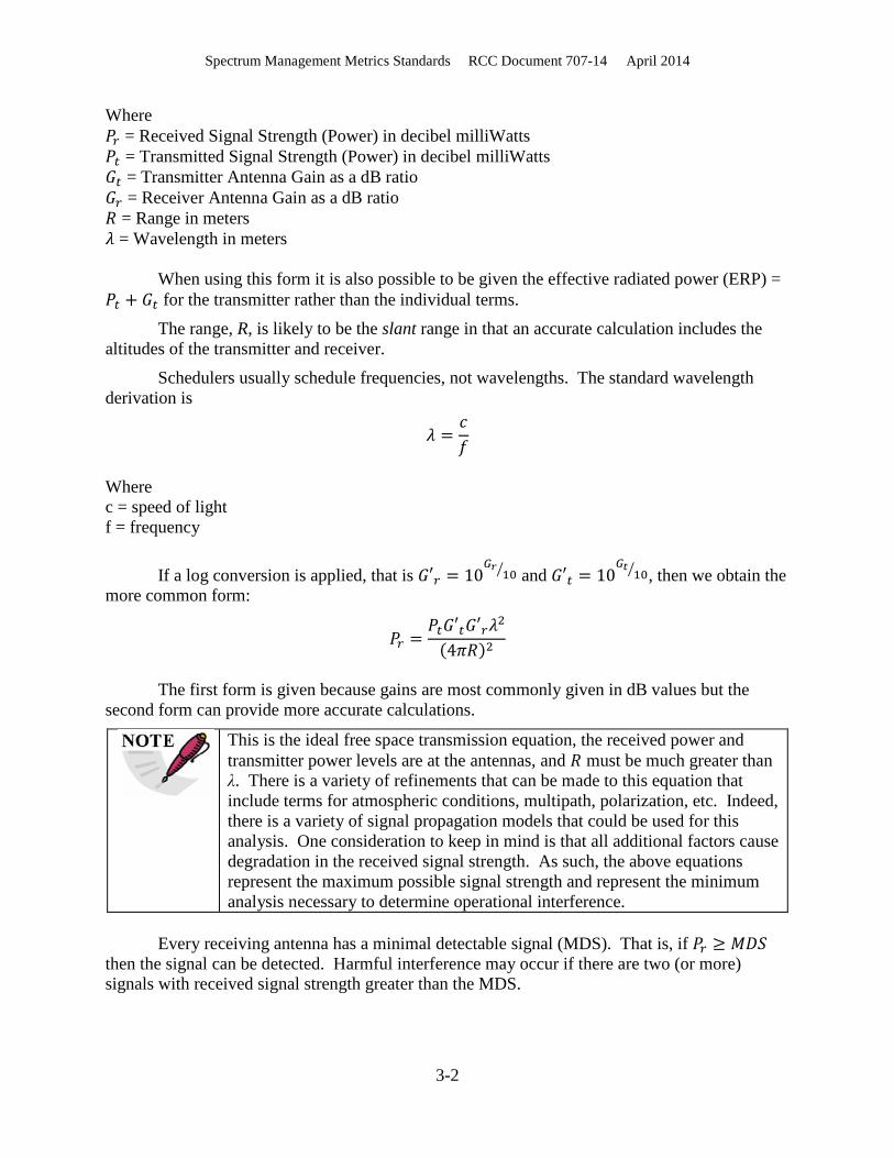
Where 𝑃𝑟 = Received Signal Strength (Power) in decibel milliWatts 𝑃𝑡 = Transmitted Signal Strength (Power) in decibel milliWatts 𝐺𝑡 = Transmitter Antenna Gain as a dB ratio 𝐺𝑟 = Receiver Antenna Gain as a dB ratio 𝑅 = Range in meters 𝜆 = Wavelength in meters

When using this form it is also possible to be given the effective radiated power (ERP) = 𝑃𝑡 + 𝐺𝑡 for the transmitter rather than the individual terms.

The range, R, is likely to be the slant range in that an accurate calculation includes the altitudes of the transmitter and receiver.

Schedulers usually schedule frequencies, not wavelengths. The standard wavelength derivation is

𝜆 =𝑐𝑓

Where c = speed of light f = frequency

If a log conversion is applied, that is 𝐺′𝑟 = 10𝐺𝑟

10� and 𝐺′𝑡 = 10𝐺𝑡

10� , then we obtain the more common form:

𝑃𝑟 =𝑃𝑡𝐺′𝑡𝐺′𝑟𝜆2

(4𝜋𝑅)2

The first form is given because gains are most commonly given in dB values but the

second form can provide more accurate calculations.

This is the ideal free space transmission equation, the received power and transmitter power levels are at the antennas, and 𝑅 must be much greater than λ. There is a variety of refinements that can be made to this equation that include terms for atmospheric conditions, multipath, polarization, etc. Indeed, there is a variety of signal propagation models that could be used for this analysis. One consideration to keep in mind is that all additional factors cause degradation in the received signal strength. As such, the above equations represent the maximum possible signal strength and represent the minimum analysis necessary to determine operational interference.

Every receiving antenna has a minimal detectable signal (MDS). That is, if 𝑃𝑟 ≥ 𝑀𝐷𝑆

then the signal can be detected. Harmful interference may occur if there are two (or more) signals with received signal strength greater than the MDS.


3-3

3.1.2 Line of Sight Most TM transmitters used require free-space line of sight between transmitter and

receiver. That is, any physical barrier such as buildings, mountains, or the curvature of the earth will block transmission. In this case, Pr = 0. The Terrain Integrated Rough Earth Model is the accepted standard for determining line of sight. This model incorporates rough earth characteristics, knife-edge diffraction, and sky-wave propagation to theoretically predict the received signal strength. In order to do this analysis it is necessary to know the receiver’s and transmitter’s respective latitude, longitude, and altitude.

3.1.3 Closest-Point Analysis The path of a transmitting test vehicle, especially airborne vehicles, is not usually

precisely planned. Further, logistical considerations limit the time precision of where a vehicle will be. As such, the geographic location of a vehicle during a test is defined in terms of general geographic area. Operational interference is thus determined on the assumption that during a test the test vehicle will come as close as possible, while staying inside the test area, to an antenna outside the test area.

An example method of determining the closest point of a test area to an antenna outside the test area is given using a polygonally defined test area. This is the most common method for defining a test area. Other methods, such as center and radius, might be used or a specific flight path might be known. Further, a more accurate analysis can be done by including altitudes of the antennas. The example method can easily be modified to those cases using standard geometry.

A polygonal area is defined by the latitude and longitude of the vertices of the polygon.

{(𝑥𝑖,𝑦𝑖) ∶ 𝑖 = 1, … , 𝑛}

The vertices are sequenced around the polygon such that lines drawn between the vertices, in sequence, form the polygon.

𝑃 = {𝑙𝑖 = (𝑥𝚤,𝑦𝚤)(𝑥𝚤+1,𝑦𝚤+1)�� ∶ 𝑖 = 1, … ,𝑛 + 1; (𝑥1,𝑦1) = (𝑥𝑛+1,𝑦𝑛+1)}

Where the over bar indicates a line segment between the two vertices.

Let (𝑥′,𝑦′) be the latitude and longitude of the receiving antenna. The closest point of the polygon to the antenna will necessarily be on the edge of the polygon. The distance between a point on a line, (𝑥,𝑦) ∈ 𝑙𝑖, and the antenna is given by:

𝑑 = �(𝑥 − 𝑥′)2 + (𝑦 − 𝑦′)2.

Thus the closest point of the test area to the antenna is the point that satisfies the condition

𝑚𝑖𝑛 {�(𝑥 − 𝑥′)2 + (𝑦 − 𝑦′)2 ∶ (𝑥,𝑦) ∈ 𝑃}.

3.1.4 Mobile and Stationary Both the receiver and transmitter may be mobile or stationary. The line-of-sight and

closest-point analysis must be modified using standard geometry to accommodate the appropriate conditions.


3-4

3.1.5 Determining Operational Interference Given a scheduled test with a transmitter and targeted receiving antenna, operational

interference occurs when a secondary transmission potentially causes harmful interference at the receiving antenna. Thus, whenever a new transmission is to be added to an existing schedule, an analysis must be made to determine if the new transmission will cause operational interference with already-scheduled tests.

Inputs to the process of determining operational interference are:

1. Receiver Parameters a. Antenna Gain b. Minimal Detectable Signal

2. Parameters for Each Transmitter

a. Time Window of Transmission b. Frequency Range (either center frequency and bandwidth or upper and lower

frequency bounds) c. Signal Strength and Antenna Gain or ERP (for the new transmitter only)

3. Location of Receiver and New Transmitter

a. Stationary i. Latitude

ii. Longitude iii. Elevation

b. Moving i. Test Area

ii. Max Altitude

The process to determine if a potential new transmission would cause operational interference for a scheduled test with a transmitter and targeted receiver is as follows.

1. Determine if the transmissions will overlap in time. If not, then there is no operational interference and no more analysis is necessary.

2. Determine if the transmissions overlap in frequency (see note below). If the frequencies do not overlap then there is no operational interference and no more analysis is necessary.

3. Determine if there is any point in the test areas where the receiving antenna and new transmitting antenna are in line of sight. If there is no such point, then there is no operational interference with that antenna and no more analysis is necessary.

4. Determine the closest line-of-site point between the receiver and new transmitter. 5. Calculate the signal strength of the new transmission at the receiving antenna using the

Friis Transmission Equation (or a more detailed signal propagation model if desired). 6. If the calculated signal strength is greater than the MDS of the receiving antenna, then the

new transmission would cause operational interference during the scheduled test.

All TM uses a contiguous range of frequencies rather than a single frequency. Further, the Friis equation shows that the received signal strength, Pr, increases with the square of the wavelength of the signal, λ. Thus, a worst-case analysis uses the highest wavelength of the transmitted frequency range.


3-5

From a practical scheduling point of view, it may be more efficient to calculate whether

𝑃𝑟 ≥ 𝑀𝐷𝑆 for each (receiver, transmitter) pair for every targeted receiver and every planned transmission. This information can then be used to develop non-interfering schedules.

3.2 Area of Mutual Use

A set of geographic areas that require test schedules to be coordinated due to operational interference is called an area of mutual use (AMU).

To determine an AMU we first define a schedulable test area as a contiguous geographic area for which there are organizations that schedule tests in that area (as mentioned previously, these test areas are usually defined as polygons). It is assumed that every antenna is located within a schedulable test area. This might not be strictly true in that some antennas, such as relay antennas, may not be within the geographic boundaries of where a vehicle navigates. In such cases, the antennas should be considered their own schedulable test area.

We then define a graph ⟨𝑉,𝐸⟩ where the set of vertices, 𝑉 = {𝑣𝑖}, is the set of schedulable test areas. For each schedulable test area, 𝑣𝑖, there is a set of antennas, 𝐴𝑖 = �𝑎𝑖𝑗�, that are within the schedulable test area. If a given test being conducted in a schedulable test area, 𝑣𝑖, induces operational interference at an antenna, 𝑎𝑘𝑗 in another test area, 𝑣𝑘, then we associate an edge in 𝐸. That is, 𝑣𝑖𝑣𝑘 ∈ 𝐸. In other words, those two test areas are in an AMU.

Once ⟨𝑉,𝐸⟩ is constructed, every connected subgraph represents an AMU. See Appendix A for an example.

If this analysis is done for a single test, then it provides a clear set of test areas that must coordinate spectrum scheduling during that test; however, this process is also intended to be used to define an area of spectrum reuse over a period of time (and thus multiple tests). There are a couple of approaches that can be taken in this situation. The first approach is to do the analysis for all tests conducted. One drawback is this allows a single test to drastically affect the AMU. For example, if there is a cross-country flight as part of a test, then the AMU becomes most of the country - which is not the intent of reuse analysis. The second approach is to use a typical test scenario for this analysis. Unfortunately, this involves some subjectivity in deciding what a typical scenario is. Heuristics for identifying a typical scenario include:

1. It is not a one-of-a-kind test. 2. It is not an average of all tests. 3. It is documented in a scheduling system in a manner that justifies its use for spectrum

reuse analysis.

Although the discussion is in terms of test scenarios, from a practical point of view, the analysis can be done based on a typical transmitter at known closest points of operation to antennas.

3.3 Definition of Spectrum Reuse

Spectrum is reused when the same frequency is used more than once at the same time in a Mutual Area of Use.


3-6



4-1

CHAPTER 4

Spectral Occupancy Metrics (Area Methods)

These methods look at areas in the time-frequency grid. Historically, the main usage metric has been PO. The descriptions below formally define PO and other related metrics. These measure actual occupancy of spectrum, which, as has been stated before, should not be used in isolation from other metrics when analyzing utilization.

4.1 Overview

4.1.1 Counting Cells Existing practical scheduling systems break both time and frequency into discrete

segments. For example, IFDS smallest time unit is 15 minutes and its smallest frequency unit is 500 kHz. This breaks the time-frequency grid into discrete cells. Calculating areas can thus be done by counting cells. This is the basic approach for the metrics in this section. For example, the left-most mission scheduled in Figure 1-1 occupies 20 cells. Each cell is 5 MHz by 1 hour or 5 MH. Thus, that mission occupies 100 MH.

4.1.2 Assumptions The fundamental assumption used in defining occupancy metrics is that metric

calculations are always over a given range of time and frequency. Most often, the frequency range will be one of the standard frequency bands. Standard time ranges will depend on particular analyses needs.

4.2 Percent Occupancy with Reuse

Occupancy for a given mission is calculated by multiplying the bandwidth of the TM transmitter by the number of hours of operation. The result, in MH, provides a quick quantification of the mission’s spectral resources consumption. Percent occupancy with reuse (POWR) is the sum of all such mission occupancies divided by the total available occupancy over the specified time and frequency ranges.


1. A high POWR (near or above 1) indicates large spectrum usage and high reuse. 2. A low POWR (near 0) indicates low spectrum usage and low reuse. 3. POWR = PO implies no reuse. 4. Due to possible reuse of frequencies (e.g., because of geographic separation), POWR can

be greater than 100%.

The POWR shall be calculated using methods mathematically equivalent to the following algorithm.

4.2.1 Predetermined Inputs to the Algorithm 1. The set of scheduled mission profiles, },...,1:),{( nibd ii = . 2. The total available frequency, F, in MHz.


4-2

3. The total available time, T, in hours.

4.2.2 Algorithm 1. For all mission profiles, ),( ii bd , calculate the mission occupancy, iii dbMO ×= .

2. TF

MOPOWR ni

i

×=∑= ,...,1 .

4.2.3 Example Using the missions scheduled in Figure 1-3, we have:

Four mission profiles: {(2, 50), (7, 10), (5, 5), (3, 35)}; A total available frequency of 95 MHz; A total available time of 14 hours. The mission occupancies are {100, 70, 25, 105).

23.01330300

1495300

==×

=POWR or 23%.

4.3 Average Percent Occupancy with Reuse

The POWR is fundamentally defined in terms of activity over a single day (although it can be defined over any time range). It is useful to consider the average daily POWR. This simply requires averaging the POWR for each day.


Average monthly POWR is the average of the daily average over each month. Similarly,

average yearly POWR is the average of the daily average over each year. This is an important distinction since the average of several averages is not usually equivalent to the average of all individual numbers.

Average POWR shall be calculated using methods mathematically equivalent to the following algorithm.

4.3.1 Predetermined Inputs to the Algorithm POWR for each day, },...,1:{ niPOWRi = .

4.3.2 Algorithm

Average daily POWR =n

POWRni∑1 .

4.3.3 Average Monthly Percent Occupancy with Reuse over Several Months 1. Calculate average daily POWR for each month.


4-3

2. Average these averages.

4.3.4 Average Yearly Percent Occupancy with Reuse over Several Years 1. Calculate average daily POWR for each year. 2. Average these averages.

4.4 3D Average Percent Occupancy with Reuse Chart

The algorithm in this section produces a chart that displays average POWR over a time-frequency grid. Given a time range and a frequency range, the grid is divided into cells. For each of these cells, average POWR is calculated. The frequency range would normally be a full contiguous band and the time range would normally be a full day or a working day or night. The algorithm presented is based on averaging over days, but it could be adapted to any time period.

3D average POWR shall be calculated using methods mathematically equivalent to the following algorithm.

4.4.1 Predetermined Inputs to the Algorithm 1. Available frequency range 2. Available mission time range 3. Scheduled missions for each day

4.4.2 Data Structures Required The schedule grid is a 2D array containing a real number for each cell in the time-

frequency grid. Thus the size of the grid is (time range / ∆T) X (frequency range / ∆B).

4.4.3 Algorithm Initialize each element of the schedule grid to 0 // Construct the raw values in the schedule grid. for each mission

Add the mission to the schedule grid by incrementing each cell the mission is scheduled in. // This is equivalent to Subalgorithm 1d. in Section 2.7.1.

end for each mission // Convert each value in the schedule grid to an average. for i=0 to maximum time index

for j=0 to maximum frequency index schedule grid [i][j] = (schedule grid [i][j] / num of days)

end for j end for i


4-4

4.4.4 Example An example raw-value grid can be constructed by adding a 0 to every empty cell in the

grid shown in Figure 1-3. In the case of averaging over only 1 day, this is also the final average POWR grid. The associated 3D average POWR chart is shown in Figure 4-1.

Figure 4-1. 3D Percent Occupancy with Reuse Chart for Figure 1-3

4.5 Percent Occupancy

This is similar to POWR but disregards any reuse of frequencies. A visualization technique would be to consider Figure 1-3 with all occupied cells having density 1.


1. A high PO (close to 1) indicates a high spectrum usage. 2. A low PO (close to 0) indicates low spectrum usage. 3. PO is always between 0 and 1. 4. It is always the case that POWRPO ≤ .

Calculation for PO shall use methods mathematically equivalent to the following algorithm.

4.5.1 Predetermined Inputs to the Algorithm 1. The set of scheduled mission profiles, },...,1:),{( nibd ii = . 2. The associated set of scheduled times and center frequencies, },...,1:),{( nift ii = 3. Available frequency range 4. Available mission time range 5. Delta time 6. Delta bandwidth

2200

2210

2220

2230

2240

2250

2260

2270

2280

2290

0:004:00

8:0012:000%

50%100%150%200%250%300%

Frequency

Time


4-5

4.5.2 Data Structures Required The schedule, ],[ jigrid , is a 2D array containing a real number for each cell in the time-


4.5.3 Algorithm // Construct the schedule by placing each mission into the schedule grid. for i = 1 to n // for each scheduled mission

end start time = it + id − ∆T

lowest center frequency = 2

ii

bf −

highest center frequency = −+2

ii

bf ∆B

for time index = scheduled start time to end start time step ∆T for frequency index = lowest center frequency to highest center frequency step ∆B

if grid (time index, frequency index) = 0 increment grid [time index, frequency index]

end if end for frequency index

end for time index end for i //for each scheduled mission Calculate the number of occupied cells, ∑=

jijigridN

,

],[ .

Calculate the cell size in MH, dBdTCS ×= . Calculate the total available frequency in MHz, F. Calculate the total available time in hours, T. Calculate PO.

TFCSNPO××

=

4.5.4 Example In the example of Figure 1-3, there are 44 occupied cells with a cell size of 5 MH. The

total available frequency is 95 MH and total available time is 14 hours. Thus, PO = (44 x 5) / (95 x 14) = 0.17 or 17%.

4.6 Average Percent Occupancy

The PO is fundamentally defined in terms of activity over a single day (although it can be defined over any time range.) It is useful to consider the average daily PO. This simply requires averaging the PO for each day.


4-6


Average monthly PO is the average of the daily average over each month. Similarly,

average yearly PO is the average of the daily average over each year. This is an important distinction since the average of several averages is not usually equivalent to the average of all individual numbers.

Average PO shall be calculated using methods mathematically equivalent to the following algorithm.

4.6.1 Predetermined Inputs to the Algorithm PO for each day, },...,1:{ niPOi = .

4.6.2 Algorithm

Average daily PO =nPOn

i∑1 .

4.6.3 Average Monthly Percent Occupancy over Several Months 1. Calculate average daily PO for each month. 2. Average these averages.

4.6.4 Average Yearly Percent Occupancy over Several Years 1. Calculate average daily PO for each year. 2. Average these averages.

4.7 3D Average Percent Occupancy

This chart displays average PO over a time-frequency grid. Given a time range and a frequency range, the grid is divided into cells. For each of these cells, average PO is calculated. The frequency range would normally be a full contiguous band and the time range would normally be a full day or a working day or night. The algorithm presented is based on averaging over days, but it could be adapted to any time period.

The value for 3D average PO shall be calculated using methods mathematically equivalent to the following algorithm.

4.7.1 Predetermined Inputs to the Algorithm 1. Available frequency range 2. Available mission time range 3. Existing scheduled missions for each day


4-7

4.7.2 Data Structures Required Each of the following grids is a 2D array containing a real number for each cell in the

time-frequency grid. Thus the size of the grid is (time range / ∆T) X (frequency range / ∆B).

1. Schedule grid 2. Average PO grid

4.7.3 Algorithm Initialize each element of the average PO grid to 0 // Construct the raw values in the schedule grid. for each day

Initialize each element of the daily schedule grid to 0 for each mission

Add the mission to the schedule grid by incrementing each cell the mission is scheduled in. // This is equivalent to Subalgorithm 1d. in Section 2.7.1.

end for each mission

// Transfer occupancy in each cell (less reuse) to the average PO grid

for i=0 to maximum time index for j=0 to maximum frequency index

if daily schedule grid[i][j] > 0 then increment average PO grid [i][j]

end for j end for i

end for each day // Convert each value in the schedule grid to an average. for i=0 to maximum time index

for j=0 to maximum frequency index average PO grid [i][j] = average PO grid [i][j] / num of days

end for j end for i

4.7.4 Example An example raw-value grid can be constructed by adding a 0 to every empty cell in the

grid shown in Figure 1-3. The transfer to the raw PO grid can be accomplished by changing each occupied cell value to 1. In the case of averaging over only 1 day, this is also the final average PO grid. The associated 3D average PO chart is shown in Figure 4-2.


4-8

Figure 4-2. 3D Percent Occupancy Chart for Figure 1-3

4.8 Percent Multiple Use

Not only does POWR include reuse, but it includes PO as well. It is useful to have a metric that captures only reuse. Thus, percent multiple use (PMU) is defined to be the amount of spectrum used more than once. A more granular method for capturing reuse is PMU(n), which is defined to be the amount of spectrum used exactly n times. This leads to the following relationships.

∑>

=1

)(n

nPMUPMU

∑>

=0

)(n

nnPMUPOWR

∑>

=0

)(n

nPMUPO

The PMU(n) shall be calculated using methods mathematically equivalent to the following algorithm.

4.8.1 Predetermined Inputs to the Algorithm 1. The set of scheduled mission profiles, },...,1:),{( mibd ii = . 2. The associated set of scheduled times and center frequencies, },...,1:),{( mift ii = 3. Available frequency range 4. Available mission time range 5. Delta time 6. Delta bandwidth

2200

2210

2220

2230

2240

2250

2260

2270

2280

2290

0:004:00

8:0012:000%

20%40%60%80%

100%

Frequency

Time

3D PO Chart


4-9

4.8.2 Data Structures Required The schedule, ],[ jigrid , is a 2D array containing a real number for each cell in the time-


4.8.3 Algorithm // Construct the schedule by placing each mission into the schedule grid. for i = 1 to m // for each scheduled mission

end start time = it + id − ∆T

lowest center frequency = 2

ii

bf −

highest center frequency = −+2

ii

bf ∆B

for time index = it to end start time step ∆T for frequency index = lowest center frequency to highest center frequency step ∆B

increment grid [time index, frequency index] end for frequency index

end for time index end for i // for each scheduled mission Calculate the number of cells used n times, ∑

=

=njigrid

jigridN),(

],[ .

Calculate the cell size in MH, dBdTCS ×= . Calculate the total available frequency in MHz, F. Calculate the total available time in hours, T. Calculate PMU(n).

TFCSNnPMU××

=)(

4.8.4 Example Figure 1-3 shows an example schedule grid after being filled with all missions. That

example has 30 cells used exactly once, 11 cells used twice, and 2 cells used three times. Thus,

CS = 5 MH F = 95 MHz T = 14 hours PMU(1) = 11.3% PMU(2) = 4.1%

PMU(3) = 0.8% PMU = 4.9%


4-10

4.9 Frequency Reuse Ratio

Frequency reuse ratio (FRR) is the ratio of POWR and PO. This provides an indication of how much spectrum is reused.


1. A large FRR indicates a high spectrum reuse. 2. FRR ≥ 1

4.9.1 Derivation of Frequency Reuse Ratio

POPOWRFRR =

4.9.2 Example Using the numeric example for PMU we have

POWR = 21.9% PO = 16.2% FRR = 21.9% / 16.2% = 1.35


5-1

CHAPTER 5

Efficiency Metrics As technology has advanced, spectrum usage has become more efficient. There are two

forms of efficiency increases addressed in this section: advances in transmitter technology and advances in scheduling technology. The most notable form of transmitter advances is through the development of new modulation methods. Specifically, more efficient modulation methods allow transmitting more bits per second (bps) in the same bandwidth. For example, shaped offset quadrature phase shift keying (SOQPSK) is known to be more efficient than pulse code modulation/frequency modulation (PCM/FM). Advances in scheduling technology include implementation of cooperative scheduling software (such as IFDS), use of terrain and signal propagation models, and changes in methods and algorithms used for scheduling.

The metrics in this section are intended to allow analysis of efficiency improvements from implementation of these technological improvements.

5.1 Scheduled Bandwidth vs. Necessary Bandwidth

The distinction between scheduled efficiency and modulation efficiency centers around the fact that the bandwidth scheduled for a given transmission is usually larger than what is sometimes called necessary bandwidth, which is the minimum emission bandwidth that allows for an acceptable quality of performance for that given transmission. Necessary bandwidth could be used if there were only a single transmission to be scheduled. Unfortunately, in a multi-transmission environment, it is necessary to provide additional spacing between transmissions in order to avoid operational interference.

Any spectrum efficiency metric is fundamentally related to bit rates (bps transmitted) and the bandwidth used for a given bit rate. In addition to formalizing the distinction between necessary bandwidth and scheduled bandwidth in the following, the distinction between modulation efficiency and scheduled efficiency takes into consideration that a transmitter does not care what the duration of a transmission is, whereas a scheduler does. Thus the two units that will be utilized for the efficiency metrics will be bps/Hz and bps/MH.

5.1.1 Necessary or 99 Percent Power Bandwidth Table A-2 of IRIG Standard 106-13 Appendix A4 provides coefficients for calculating

necessary bandwidth. (Note that within IRIG 106, necessary bandwidth is synonymous with 99% power bandwidth.) That is, given a bit rate, R, and the coefficient for a particular modulation method, BP, then the necessary bandwidth is BN = BPR.

Note that the necessary bandwidth calculation for analog (vs. digital) transmitters for PCM/FM can be affected by the transmitter’s filtering ability. For analog transmitters, the digital data from the data system is externally filtered and amplitude adjusted prior to the transmitter in order to provide the correct modulation index for PCM/FM. Row entries with appropriate variants are included in Table A-2 in IRIG Standard 106-13 Appendix A.

4 Range Commanders Council. Telemetry Standards. Appendix A, Frequency Considerations for Telemetry. A-10, Table A-2. IRIG Standard 106-13. June 2013. Available at http://www.wsmr.army.mil/RCCsite/Documents/106-13_Telemetry_Standards/appendixA.pdf.

http://www.wsmr.army.mil/RCCsite/Documents/106-13_Telemetry_Standards/appendixA.pdf



5-2

5.1.2 Scheduled Bandwidth To schedule transmissions in a multi-transmission environment it is necessary to consider

factors that can create operational interference. Examples include acceptable interference criteria, adjacent channel interference criteria, filtering capabilities of the TM receiver, transmit and receive antenna directionality, and many other factors. This manifests itself in the need to space transmissions wider than might be done if only necessary bandwidth were considered.

Standards for calculating this signal spacing can be found in IRIG 106. Due to the granularity of channelization within each frequency band, there might also be some rounding in center-to-center spacing. Further, individual schedulers may have specific requirements and policies that affect this spacing. Thus, scheduled bandwidth is what is actually scheduled due to practical considerations rather than the more theoretical and restricted necessary bandwidth.

Just as improvements in modulation techniques are increasing modulation efficiency, improvements in technology may allow decreasing the scheduled spacing requirements. This version of this standard does not address this potential change in efficiency, but it may be worth evaluating for future versions.

5.2 Mission Modulation Efficiency

Given the bit rate, R, and the necessary bandwidth, b, of a mission, mission modulation efficiency (MME) is defined as:

MME = R/b For example, given R = 15 megabits per second (Mbps) and b = 20 MHz, then MME =

15/20 = 0.75 bps/hertz.

5.3 Average Mission Modulation Efficiency

Average mission modulation efficiency (AMME) is the average of a set of MMEs.

Calculation of AMME shall use methods mathematically equivalent to the following algorithm.

5.3.1 Predetermined Inputs to the Algorithm 1. A set of necessary mission bandwidths in MHz, �𝑏�: 𝑖 = 1, … ,𝑛�. 2. The associated bit rate for each mission, {𝑅𝑖: 𝑖 = 1, … , 𝑛}.

5.3.2 Algorithm

AMME = n

Rbni ii∑ = ,...,1

ˆ

5.4 Modulation Method Ratio

This metric is based simply on counting transmitters and their ability to transmit using a particular modulation method. This can be used to track the progress of upgrading test vehicles


5-3

with newer transmitters; however, not all modulation methods are adequate for use under all conditions (for example, some methods are more susceptible to multipath than others). Thus, just because a transmitter is capable of using a modulation method, it does not mean the method was actually used during a test. This ratio could therefore be used to quantify actual modulation usage in contrast to modulation capability.

The modulation method ratio is the number of transmitters using (or capable of using) a given modulation method divided by the total number of transmitters.

5.5 Mission Spectrum Efficiency

Given the bit rate, R, the scheduled bandwidth, b, and the duration, d, of a mission, mission spectrum efficiency (MSE) is defined as:

MSE = R/b/d

For example, given R = 15 Mbps, b = 20 MHz, and d = 5 hours, then MSE = 15/20/5 = 0.15 Mbps/MH.

5.6 Average Mission Spectrum Efficiency

Average mission spectrum efficiency (AMSE) is the average of a set of MSEs.

Calculation of AMSE shall use methods mathematically equivalent to the following algorithm.

5.6.1 Predetermined Inputs to the Algorithm 1. A set of scheduled mission bandwidths in MHz, },...,1:{ nibi = . 2. The associated scheduled mission bandwidths in hours, },...,1:{ nibi = . 3. The associated bit rate for each mission, },...,1:{ niRi = .

5.6.2 Algorithm

AMSE = n

dbR ini ii //,...,1∑ =

5.7 Average Spectrum Band Efficiency

Average spectrum band efficiency (ASBE) looks at MSE in relation to an entire spectrum band. If there is only one mission scheduled in a band, AMSE might be very high, but the amount of unused spectrum would generate a very low ASBE. This can also be calculated over multiple bands.

Calculation of ASBE shall use methods mathematically equivalent to the following algorithm.

5.7.1 Predetermined Inputs to the Algorithm 1. The bit rates for a set of missions, },...,1:{ niRi = .


5-4

2. The total available frequency, F, in MHz. 3. The total available time, T, in hours.

5.7.2 Algorithm

ASBE = FTn

Rni i∑= ,...,1

5.8 Bits Sent

Adding up the number of bits sent can answer the question: Is the amount of data being transmitted increasing?

Bits sent shall be calculated using methods mathematically equivalent to the following algorithm.

5.8.1 Predetermined Inputs to the Algorithm 1. A set of mission durations in seconds, },...,1:{ nidi = . 2. The associated bit rate, in bps, for each mission, },...,1:{ niRi = .

5.8.2 Algorithm Bits Sent = ∑ = ni iiRd

,...,1

5.9 Bits Sent per Megahertz Hours

Bits sent and ASME do not take into consideration unscheduled spectrum or reused spectrum, whereas bits sent per MH does. This can be used for trend analysis capturing an increase in overall usage that incorporates improvements in modulation methods and spectrum scheduling. This can answer the question: Is the amount of data being transmitted per unit of available spectrum increasing?

Bits sent per MH shall be calculated using methods mathematically equivalent to the following algorithm.

5.9.1 Predetermined Inputs to the Algorithm 1. A set of mission durations in seconds, },...,1:{ nidi = . 2. The associated bit rate, in bps, for each mission, },...,1:{ niRi = . 3. The total available frequency, F, in MHz. 4. The total available time, T, in hours

5.9.2 Algorithm

Bits Sent per MH = TF

Rdni ii

×∑ = ,...,1


6-5

CHAPTER 6

Metrics by Mission Groupings

The metrics defined elsewhere generally use single missions as base units; however, there are groupings of missions that provide useful analysis. In particular, an operation consists of multiple missions required to implement a particular test. Other examples of groupings are by job order number or by user. The following metrics are defined in terms of operations, but are applicable to other groupings.

It is also possible to calculate other metrics, such as PO or PMU, by using the appropriate algorithm on just the members of the group.

6.1 Operation Size

There are three sizes to consider: duration, bandwidth, and MH. Because some missions within an operation may overlap (in time or frequency), there is no inherent relation between these total operation sizes.

Operation sizes shall be calculated using methods mathematically equivalent to the following algorithm.

6.1.1 Predetermined Inputs to the Algorithm Set of mission profiles in the operation, },...,1:),{( mibd ii = .

6.1.2 Algorithm Operation duration = ∑

= miid

,...1

Operation bandwidth = ∑= mi

ib,...1

Operation MH = ( )∑=

×mi

ii db,...1

6.2 Operational Statistics

Among many possible statistics that could be generated, averages and maximums of the following are noted in particular.

1. Number of missions per operation 2. Number of frequency bands used per operation 3. Operation duration 4. Operation bandwidth 5. Operation MH


6-6



7-1

CHAPTER 7

Scheduling Operational Metrics

7.1 Requests Authorized

A major reason for the existence of this standard is that not all requests for assignments are being authorized. In order to quantify how well requests are being met, a definition of a request is defined and then several levels of authorization are established.

7.1.1 Spectrum Request A single-assignment request shall include:

1. The required mission duration; 2. The required bit rate; 3. The transmitter capabilities;

a. Modulation methods (e.g., PCM/FM, SOQPSK, etc.); b. Frequency tenability;

4. Acceptable start times including days and hour ranges.

A spectrum request shall include a set of single-assignment requests needed for a single operation.

Using this request information, a set of mission assignments is determined. Bandwidth is determined using a combination of the bit rate, the 99% power bandwidth of the modulation method (as identified in Table A-2 in IRIG Standard 106-13 Appendix A), and technical considerations related to interference. The start time and center frequency are determined in consideration with all requests submitted, schedule availability, and operational priorities.

7.1.2 Approval Categories The following categories of approval are defined.

1. Request Authorized - The assignments requested were scheduled in the requested start times and frequencies.

2. Request Authorized Through Coordination and Deconfliction - The assignments were scheduled at times and frequencies not part of the original request but with no impact to the requesting organization.

3. Request Authorized but at Impact to The Requesting Organization -The assignments were scheduled at times and frequencies not part of the original request but with impact to the requesting organization. Impacts include cost, schedule, or reduction of testing functionality.

4. Requests Not Authorized - The assignments could not be scheduled due to lack of spectrum availability.

7.2 Assignment Canceled, Delayed, or Rescheduled

Once an assignment is scheduled it is possible for it to be canceled, delayed, or rescheduled. A percentage of each is useful at some level, but an understanding of why these


7-2

actions happen will provide means for developing methods for avoiding these incidents in the future.

7.2.1 Categories The following categories are established.

1. Canceled - The assignment is eliminated from the schedule and not rescheduled at the time of the cancellation. A future request to reschedule shall be considered a new request.

2. Delayed - The assignment was not implemented at the time originally scheduled but started within the original scheduled duration.

3. Rescheduled - The assignment was canceled but rescheduled at a later time.

7.2.2 Reasons The following reasons for cancellation, delay, or rescheduling are established.

1. Bumped - An operation with higher priority was scheduled when the assignment was originally scheduled.

2. Operational Difficulties - The organization requesting the operation was not able to implement the mission at the time or frequency scheduled.

3. Other - Any other reason. This shall include a comment field. Users that have established codes for cancellations or other schedule changes should provide those codes in this field.

7.3 Assignment and Operation Statistics

Among many possible statistics that could be generated, the following are noted in particular.

1. Total number of operations scheduled, cancelled, delayed, and rescheduled 2. Total number of operations requested 3. Each satisfaction category as a percentage of the total number of spectrum requests over a

given time period 4. Canceled, delayed, and rescheduled missions as a percentage of the total number of

missions over a given time period


8-1

CHAPTER 8

Predictive, What If, Metrics

The allocation of spectrum is not static. The spectrum that is used for T&E can be, and has been, changed in terms of the actual frequencies and the quantity of spectrum allocated. Further, test programs come and go so that spectrum requirements change constantly. These metrics attempt to quantify the ability to meet future spectrum needs. The approaches provided assume there is historical data available and, in some instances, an estimate of future requirements in terms of both increases and decreases to historical usage. Suggested analyses include the following.

1. Evaluate ability to meet requirements when spectrum is de-allocated. This may include relocation to another band or simply loss of spectrum for federal use.

2. Evaluate impact of new requirements, most likely in the form of a large future program. 3. Evaluate effect of technology advances, in particular modulation efficiency

improvements. If a new modulation technique is known to reduce scheduled bandwidth requirements per mission, then the known reduction can be applied to historical data in order to quantify an overall reduction in spectrum requirements.

4. Evaluate impact on cost, schedule, and performance on test programs due to lack of sufficient spectrum. A predictive analysis can provide insight into how much a test program might have to extend its program (calendar time) or how much testing must be reduced.

8.1 Spectrum Movement Analysis

Two methods are provided for analyzing the impact of moving spectrum activity from one band to another. This is useful when it is necessary to relocate out of a band.

8.1.1 Additive Method This method can be used with PO, POWR, or utilization; each has its own advantages

and disadvantages. When using this method, it is important to understand that POWR is additive without constraint. In contrast, PO is additive only under the assumption that all assignments can be scheduled in the new band. This is most often not a true assumption due to the difficulties of scheduling. Utilization is not strictly additive since it includes fragmentation, which will change depending on how assignments are (or can be) scheduled. A reasonable assumption is that the additive method for PO provides a lower bound and the additive method for utilization provides an upper bound for utilization in the new band.

The main assumption of this method is that mission requests will be similar in the future to those made in the past.

Additive spectrum movement analysis shall be calculated using methods mathematically equivalent to the following algorithm.

8.1.1.1 Algorithm Outline 1. Calculate average utilization or PO over an historical time period in both the band to be

vacated and the band to be moved into. 2. Normalize these averages to MH.


8-2

3. Add the normalized averages and de-normalize to a percentage in the band to be moved into.

8.1.1.2 Predetermined inputs to the algorithm 1. The band to be vacated, BV, defined by upper and lower limits of frequency 2. The band to be moved into, BM, defined by upper and lower limits of frequency 3. The time range of concern for both bands 4. Historical schedules for both BV and BM

8.1.1.3 Algorithm Calculate total available occupancy for both bands by multiplying the total available bandwidth by the total possible duration. This gives TAOV and TAOM. Calculate average utilization (or PO) for both bands using the algorithm in Section 2.5 (or Section 4.5). This gives UV and UM as decimal numbers between 0 and 1. Normalize to MH: VVV TAOUU =|| and MMM TAOUU =|| Add: |||||| VMP UUU +=

De-normalize to give the predicted utilization (or PO) after the move: M

PP TAO

UU ||=

8.1.1.4 Example Assume BV = 50 MHz BM = 30 MHz The time range is a full day, 24 hours UV =22% UM =36% Then TAOV = 50 MHz * 24 hours = 1200 MH TAOM = 30 MHz * 24 hours = 720 MH | UV | = 0.22 * 1200 MH = 264 MH | UM | = 0.36 * 720 MH = 259.2 MH | UP | = 264 MH + 259.2 MH = 523.2 MH UP = 512.2 MH / 259.2 MH = 72.7%

8.1.1.5 Evaluation 1. Because of the non-additive nature of utilization, a predicted utilization of less than 100%

(or slightly higher) implies a high probability of being able to schedule all assignments in the new band.

2. A predicted utilization significantly higher than 100% (nominally greater than 115%) implies a high probability that some assignments will not be able to be scheduled in the new band.


8-3

3. Studies have shown that a PO of 60-80% is probably maximal due to fragmentation and other logistical and scheduling limitations. That is, from a practical point of view, it is difficult to achieve a PO close to 100%. Thus a predicted PO below 60% implies a high probability of being able to schedule all assignments in the new band.

4. A predicted PO above 80% implies a high probability of not being able to schedule all assignments in the new band.

This method can be used for moving into a band that has not been previously used. In

that case, UM = 0.

This method can also be used for moving only a portion of assignments into a new band. For PO, simply reduce POV to include only that portion of assignments. For utilization it is necessary to calculate UV for the schedule with all assignments and for the schedule without that portion of the assignments. After this is done, obtain UV by subtracting the two.

8.1.2 3D Additive Method This method combines the 3D utilization charts with the additive method to produce a 3D

illustration of the affect of moving spectrum utilization out of one band into another. The algorithm is given in terms of utilization, but may be applied to PO as well.

3D additive spectrum movement analysis shall be implemented as follows.

8.1.2.1 Predetermined inputs to the algorithm 1. 3D utilization chart for band being moved into 2. Average utilization for the band being moved into, UM 3. Predicted utilization for the band being moved into after the move, UP

8.1.2.2 Algorithm Calculate the average percent difference in predicted vs. actual utilization: UD = UP − UM. Increase the value in each cell of the 3D utilization chart by UD.

8.1.2.3 Example The following example is based on moving all utilization out of 2310-2360 MHz into

2360-2390 MHz. Figure 8-1 shows the original average utilization. The data is consistent with the example in Section 8.1.2. Thus, UD = 72.7% − 36% = 36.7%. Multiplying all the cells in 2360-2390 MHz by 1.362 (and vacating 2310-2360 MHz) produces Figure 8-2.


8-4

Figure 8-1. Spectrum Utilization before Move Analysis

Figure 8-2. Predicted Utilization after Move Analysis

8.1.3 Days Not Schedulable Method Instead of simply looking at averages, this method looks at each day over an historical

period to see if it would have been possible to schedule all assignments in the new band for that

2310

2320

2330

2340

2350

2360

2370

2380

2390

0:00

12:00

24:000%10%20%30%40%50%60%70%80%90%

100%

Utilization

Frequency

Time

Utilization Before Move

2310

2320

2330

2340

2350

2360

2370

2380

2390

0:00

12:00

24:000%10%20%30%40%50%60%70%80%90%

100%

Utilization

Frequency

Time

Utilization After Move


8-5

day. The algorithm described bases its decision only on mission profiles and does not take into consideration any other scheduling restrictions that may apply. As such, this represents a lower bound of days that could not be scheduled.

The basic approach is to try every combination of schedules to see if the mission profiles will fit into the new band. This means that the algorithm is computationally intensive and may take some time to run. In fact, since the number of possible combinations to try increases exponentially, a recommended limit on the number of tries is provided.

The main assumptions of this method are as follows.

1. Mission requests will be similar in the future to those made in the past. 2. Mission profiles can be scheduled at any time or frequency.

Note that this is fundamentally a brute-force approach to scheduling and, as indicated by

the second assumption, there are no constraints placed on the missions. A more realistic analysis could be made using more sophisticated algorithms that incorporate constraints such as logistical constraints of time or day, or technical constraints such as non-tunable transmitters. More sophisticated algorithms could also reduce or eliminate the exponential complexity.

Days not schedulable movement analysis shall be calculated using methods mathematically equivalent to the following algorithm.

8.1.3.1 Predetermined inputs to the algorithm 1. The band to be vacated, BV, defined by upper and lower limits of frequency 2. The band to be moved into, BM, defined by upper and lower limits of frequency 3. The time range of concern for both bands 4. Historical schedules for both BV and BM

8.1.3.2 Algorithm 1. For each day:

a. Combine all assignments of both schedules into a list of mission profiles; b. Try all possible combinations of schedules in the band to be moved into.

2. Count the number of days that could not be scheduled.

8.1.3.3 Algorithm Efficiency Notes Because of the exponential growth of possible combinations, it may not be practical to try

all combinations. The following items will make the search more efficient.

1. Check to see if the total occupancy of all the mission profiles is greater than the total available occupancy of the band to move into. If this is true, then no schedule exists and the combinations need not be tried.

2. Sort the mission profiles for each day by total MH in descending order. This makes the algorithm greedy in that it places the largest rectangles first.

It is recommended that a limit of 10,000 schedules be attempted per day. Of course, the

higher this limit, the more confidence in the final answer. Days for which a schedule is not determined shall be counted and reported.


8-6

8.1.4 Method Comparison The additive method provides an approach using averages. This smoothes the utilization

out by spreading it over large time periods. The 3D additive method provides more granularity by providing some insight into utilization by time of day. The days not scheduled method provides a different type of granularity by looking at different days.

It is possible for the average determined by the additive approach to indicate scheduling would not be a problem after the move; however, the other two analysis methods may show that, in practice, there would have to be a significant reshuffling of test activities either shifted during the day, or shifted over weeks or months. Either of these shifts could negatively impact test programs.

8.2 New Program Impact Analysis

The same methods described in Section 8.1 for spectrum movement analysis can be used to analyze the impact of future programs with a couple of differences.

1. Instead of using a band to move from, identify a set of mission requests for the new program. This includes not only standard mission profiles, but identification of how often tests will be conducted over the life of the project.

2. In most cases, this type of analysis will only be for programs that are anticipated to have large spectrum requirements. Older programs with large spectrum requirements that will have decreased requirements during the time frame under consideration should have their spectrum usage removed from the historical data.

Although the methods described provide analytic approaches to predicting future

requirements, it is incumbent upon the analyst to provide reasonable data into these algorithms. Deciding what the projected mission requests are and what historical missions should be removed should be done very carefully.


9-1

CHAPTER 9

Spectrum Management Cost Model

This chapter will be developed for future updates to this document. It will provide items to be included in a cost model regarding how much it costs to manage spectrum and what the cost to programs are when tests are cancelled, delayed, or not scheduled due to spectrum constraints.


9-2



10-1

CHAPTER 10

Standard Chart Layouts Charts shall adhere to the following unless there is an aspect of the data obscured by the

size or orientation established. All figures in this standard follow these layouts.

1. For 3D charts a. The x-axis is frequency. b. The y-axis is time. c. The z-axis is percentage. d. The frequency axis is displayed front left. e. The time axis is display front right.

2. For 2D charts a. The x-axis is time or frequency. b. The y-axis is percentage.

3. Percentage axes are scaled to 100% unless percentages are greater than 100%. 4. Frequency axis labels include the lowest and highest frequencies with other frequency

labels evenly distributed. 5. Time axis labels include the start and end times with other time labels evenly distributed. 6. Time and frequency axis labels increase left to right.


10-2



A-1

APPENDIX A

Tutorial on Interference and Spectrum Reuse

A.1 Overview

This informative appendix is intended to supplement Chapter 3. There are two aspects of frequency management that are addressed in this appendix. The first is the day-to-day practical issue of how to schedule multiple frequencies such that they do not cause interference with each other. The second is the longer-term management issue of evaluating spectrum reuse: that is, how and when the same frequencies can be used at the same time within the constraints of scheduling and geography and whether or not this is done in an optimal way. Determining interference potential is a necessary part of frequency scheduling deconfliction. The issue of reuse is more an issue of maximizing and reporting utilization; however, understanding of, and quantification of, interference potential plays an important part in defining reuse. To report reuse of a particular frequency when the two uses are 3000 miles apart is probably not appropriate reporting (except in very special circumstances) since the two users are not likely to interfere with each other. Thus, this appendix defines operational interference and how this leads to a defensible definition of reuse.

For the sake of completeness, let’s review the basic issues regarding interference. The power of RF signals propagates according to an inverse square law. That is, the power decreases in proportion to the square of the distance the signal travels. Generally we assume a spherical propagation from an omnidirectional antenna. A receiving antenna can receive the signal depending on the signal strength and the sensitivity of the receiver. In the figures below, the circle around the plane represents the sphere of propagation of the RF signal. That is, an antenna outside the circle is assumed to be unable to receive the signal.

Figure A-1 illustrates the basic situation where interference occurs. Two planes (or, more generally, transmitters) send a signal that can be received by the same receiving antenna. The most common situation is when the signals being transmitted are the same frequency; however, this is not a requirement. There is both co-channel interference and adjacent-channel interference. Further, there is the near-far problem and the issue of side lobes.


A-2

Figure A-1. Basic Interference

Figure A-2 illustrates basic non-interference. The two planes are far enough from each other’s intended receiver that they do not interfere with each other’s reception. The spheres of propagation may or may not intersect. In the case where the spheres intersect, it seems reasonable to say there is reuse since there are two sets of electromagnetic energy occupying the same physical space; however, as we will discuss later, this is a limited definition of reuse.

Figure A-2. Basic Non-Interference and Reuse


A-3

A.2 Definition of Operational Interference

Note that there are multiple definitions of interference. The foundational concept is commonly referred to as harmful interference. That is, a communication is not decodable at a receiving antenna due to the presence of a secondary signal. This might be considered interference that actually happened. In contrast, from a scheduling point of view, it is necessary to consider potential harmful interference. This we call operational interference. That is, if, during multiple test operations, the possibility exists that a transmitter will cause harmful interference to the reception of a signal from a second transmitter, then this must be taken into consideration during scheduling.

The ability to predetermine harmful interference is severely limited by the fact that flight (or, more generally, test) paths are not perfectly choreographed in time and space. At least two reasons contribute to this: 1) flights are only scheduled in large geographic areas so that most flights are flown on a see-and-avoid basis; and 2) tests are not executed exactly when scheduled due to logistical difficulties of coordinating all participants.

An extreme example of when operational interference means the difference between executing a test and not executing a test is when a flight termination system (FTS) is being used. It is not worth the risk of a vehicle self-destructing if it cannot be guaranteed that the FTS signals will not be interfered with. Even when an FTS is not in use, operational interference can severely affect scheduling. Loss of data due to any reason can mean either re-executing a test point or possibly having to re-execute the entire test. This is expensive and should be avoided.

To be explicit, operational interference - the potential for harmful interference - is the basis for scheduling. If harmful interference has occurred then it is too late and the scheduling process has failed.

A.3 Determining Operational Interference

When determining operational interference during a test, there are two main issues:

1. Where will the transmitting vehicle be during the test? 2. What is the sphere of propagation?

Specific flight plans defining exactly where a transmitting test article will be during the

entire test are not made. Although there may be specific portions of the test that provide (or require) this information, the majority of a flight test is flown on a see-and-avoid basis. The level of spatial or geographic scheduling is on the basis of large, usually polygonal (or polyhedral) flight areas. A maximum altitude limit is usually provided as well. The only time the spatial position of a transmitting vehicle is known with any precision is during some ground tests.

The IFDS calculates potential interference using a closest-point approach based on the scheduled flight area. Thus, as illustrated in Figure A-3, if there is an antenna within the sphere of propagation along the edge of the flight area, then a potential for operational interference is flagged. The sphere of propagation is determined using the Friis Transmission Equation. Another factor in determining potential interference is terrain. For the most part, the frequencies used for TM require line-of-sight between transmitter and receiver. Thus mountains or other obstructions reduce or eliminate the potential for interference. Over long distances, the curvature


A-4

of the earth can play this role. As such, for example, ground tests have a much smaller sphere of propagation than flight tests. Another way to look at this is to recognize that, due to terrain, the sphere of propagation is not truly a sphere. In this sense, it might be more proper to talk of a volume of reception rather than a sphere. To be explicit, there is only a potential for interference if there are two tests scheduled at the same time and the transmissions of one of the tests could interfere with the receiver of the other test.

Figure A-3. Closest Point in Assigned Air Space

A.4 A Refinement of the Definition of Reuse

By definition we are saying reuse is when the same frequency is used more than once in a given spatial (geographic) area. The big question is how do you define the spatial area? Some basic approaches include:

1. Test Range a. As defined by some person or group of people b. As defined by IFDS

2. Group of Test Ranges a. By area frequency coordinator b. By geographic proximity

3. Flight test area (e.g., R2508) (or group of areas) 4. Receiving antenna or group of antennas 5. Center point and radius

All of these seem somewhat arbitrary. A more defensible definition of reuse is to define

the spatial area based on the physics of transmission. Further, let us recognize that interference occurs at the point of reception. Thus it is receiving antennas that are the focal points of trying to define an area of reuse. Recall that a sphere of propagation is dependent upon both the power of


A-5

the transmitter and the sensitivity of the receiver. Thus we can invert the concept and define a sphere of reception for receivers. Starting with this, the following process builds up an AMU that could be used as the spatial area for determining reuse.

Let us define a scheduling range as some entity that has the authority to schedule frequency in some geographic space (from a practical point of view, this is likely to be a range as defined in some spectrum scheduling system such as IFDS). If a scheduling range regularly schedules an operation that intersects a sphere of reception then that sphere of reception is in the area of use for that scheduling range (see Figure A-4). Define a graph with all scheduling ranges as nodes. Two nodes are connected if the areas of use for the associated scheduling ranges intersect. An AMU is the union of the areas of use of all scheduling ranges in a connected subgraph.

Figure A-4. Area of Use

If two scheduling ranges have areas of use that intersect, it is fairly obvious that they share an AMU. In particular, consider that these two ranges must coordinate so as not to interfere with each other’s operations. What is less obvious is that, just because two ranges’ areas of use do not intersect does not mean that they do not share an AMU or, more practically, that they do not have to coordinate with each other to avoid interference. For example, if there exists a third range, R3, that intersects both of the (non-intersecting) ranges, R1, and R2, then this third range must coordinate with both of these ranges. This connectivity causes a ripple effect. A frequency used by R1 affects what frequencies R3 can use, which affects what frequencies R2 can use. An example is shown in Figure A-5.


A-6

Figure A-5. Seven Areas of Use, Two Areas of Mutual Use, and Associated Connected

Subgraphs

The main ambiguity here is what is meant by a regularly scheduled operation. This probably requires some subjective judgment (although it would be possible to establish an arbitrary set of quantifiable criteria). Two points of consideration: regular does not mean some type of average and regular does not mean a one-of-a-kind operation. Regular means something that is often enough that its regularity is documented in a scheduling system. Again, this whole process is an attempt to provide a defensible definition of reuse.

We can now define reuse as when the same frequency is scheduled in an AMU via some form of mitigation and coordination.

A scheduling range may have different AMUs for different bands or applications. For example, FTS applications would have different AMUs than non-FTS applications. In terms of bands, consider that terahertz transmission distances are measured in meters rather than the kilometers of lower frequency signals. It may also be necessary to consider mixed applications in the same band. For example, radar and TM can co-exist in the same frequencies.


B-1

APPENDIX B

Glossary Allocation (of a Frequency Band). Entry of a frequency band into the Table of Frequency

Allocations5 for use by one or more radio communication services or the radio astronomy service under specified conditions.

Area of Mutual Use. A set of geographic areas that require test schedules to be coordinated due to operational interference.

Assignment (of a Radio Frequency or Radio Frequency Channel ). Authorization given by an administration for a radio station to use an RF or RF channel under specified conditions.

Available frequency range. The contiguous set of frequencies in which a mission must be scheduled.

Available mission time range. A contiguous range of time in which a mission may be scheduled (i.e., the entire mission must be completed during that time).

Bandwidth. Width of contiguous spectrum in MHz. Usually representing the spectrum used by a single mission. Bandwidth is normally provided in increments of the minimum delta bandwidth. (A phenomenological definition of bandwidth is provided in IRIG Standard 106-13.)

Center frequency. The frequency at the center of a mission’s bandwidth. The upper and lower frequencies of a mission are calculated by adding or subtracting half of the mission’s bandwidth to the center frequency.

Band (or Frequency Band). A contiguous set of frequencies.

Delta Bandwidth. The smallest bandwidth increment for which a mission can be scheduled, denoted by ∆B.

Delta Time. The smallest time increment for which a mission can be scheduled, denoted ∆T.

Duration. Length of a mission in minutes. Durations are normally provided in increments of the minimum delta time.

Harmful Interference. When a communication is not decodable at a receiving antenna due to the presence of a secondary signal

Mission. The spectrum assigned to a user for a given duration.

Mission Profile. Bandwidth and duration of a given mission. This is denoted by (d,b) where d is the duration and b is the bandwidth. Graphically, a mission profile is a rectangular region in the time-frequency grid.

Operation. A set of missions. A normal test activity often uses more than one mission or assignment.

5The definitions of the radio services that can be operated within certain frequency bands contained in the radio regulations as agreed to by the member nations of the International Telecommunications Union. This table is maintained in the United States by the Federal Communications Commission and the National Telecommunications and Information Administration.


B-2

Operational Interference. The potential of harmful interference during a scheduled test operation due to other scheduled test operations.

Required Frequency. The frequency a mission must be scheduled on.

Schedulable (at a Start Time and Center Frequency). A mission does not conflict with any other scheduled mission at the specified start time and center frequency. Graphically, this means that the rectangle of the mission profile does not overlap the rectangle of any other mission. This term is often used in the metric algorithms where it is necessary to determine if a mission profile is schedulable at a given start time and frequency.

Start time. The time of the day when a mission starts. The end time can be determined by adding the mission’s duration to the start time.

Spectrum Reuse. When the same frequency is used more than once at the same time in an AMU

Spectrum Utilization. The portion of spectrum not available for use by operations not already scheduled. Informally this is thought of as PO plus fragmentation. It is formally defined algorithmically.


C-1

APPENDIX C

References Range Commanders Council. Frequency Management Standard Operating Procedure for

Frequency Deconfliction. RCC 706-02. March 2003. May be superseded by update. Available at http://www.wsmr.army.mil/RCCsite/Pages/Publications.aspx.

———. Telemetry Standards. IRIG 106-13. June 2013. May be superseded by update. Available at http://www.wsmr.army.mil/RCCsite/Documents/106-13_Telemetry_Standards/.

———. Telemetry Standards. Appendix A, Frequency Considerations for Telemetry. A-10, Table A-2. IRIG 106-13. June 2013. Available at http://www.wsmr.army.mil/RCCsite/Documents/106-13_Telemetry_Standards/appendixA.pdf.

http://www.wsmr.army.mil/RCCsite/Pages/Publications.aspx






C-2

* * * END OF DOCUMENT * * *