Do Rural Roads Create Pathways out of Poverty?

Evidence from India ∗

Shilpa Aggarwal†

November 14, 2013

Abstract

This paper studies the impact of road provision on investments in physical andhuman capital in rural areas. The context is a large scale road construction programin rural India. Using data from household surveys and agricultural markets, the paperprovides 2 main pieces of reduced form evidence. First, beneficiary farmers were morelikely to adopt new technologies, such as chemical fertilizer and hybrid seeds. Second,teenaged children were more likely to drop out of school and join the labor force. Iargue that these changes stemmed from altered relative prices, as there is evidence ofreduced price dispersion in areas that got more roads. There is also evidence of changesto the household consumption mix.

JEL Classification: O18, J24, Q16, R42, F14

∗I am immensely grateful to Jonathan Robinson for an abundance of guidance and support. This paper hasbenefited substantively from feedback provided by Carlos Dobkin, Jennifer Poole, Nirvikar Singh, and AlanSpearot. I thank S Anukriti, Manuel Barron, George Bulman, Lorenzo Casaburi, Arun Chandrasekhar, JesseCunha, Pascaline Dupas, Ben Faber, Rob Fairlie, Fred Finan, Johanna Francis, Marco Gonzalez-Navarro,Jeremy Magruder, Justin Marion, Ted Miguel, Paul Novosad, and seminar participants at NEUDC 2013,Stanford and UC Berkeley Development Workshops, University of San Francisco, and multiple forums atUC Santa Cruz for helpful suggestions. Financial support from the UC Santa Cruz Economics Departmentis gratefully acknowledged. I thank Pankaj and Sanjay Gupta for access to the agricultural census. Thisproject would not have been possible but for the many hours spent downloading PMGSY data by BijoyBhukania and Neha Singhal. All errors are my own.†University of California, Santa Cruz, 1156 High Street, Santa Cruz, CA 95064, email: saggarw1@ucsc.edu

1 Introduction

Markets in developing economies are often characterized by spatial fragmentation due

to poor transportation infrastructure. This inhibits households’ and firms’ ability to access

goods and labor markets, technological innovations, and government services (World Bank,

2007; 2009). Policy-makers have increasingly attempted to address this problem by directing

large sums of money towards the provision of roads and railroads.1 However, the causal

impact of these investments is not well-understood as placement tends to be driven by

endogenous factors such as demand, political economy, and social objectives. This precludes

us from drawing rigorous conclusions about the first-order relationship between infrastructure

and market integration, and its subsequent bearing upon economic and social welfare.

This paper exploits a rule-based public program that led to plausibly exogenous provision

of roads in rural India, to provide four distinct pieces of evidence on the relationship between

roads and economic outcomes. Following Donaldson (2013), I start by establishing that road

construction indeed reduced transportation costs and led to greater market integration, as

dispersion of food prices declined in districts with greater road construction. I then provide

reduced form evidence on the impact of this relative price change on farms’ and households’

incentives to invest in technology adoption and human capital. Specifically, I show two

things: first, farmers in districts which received more roads increased their use of fertilizer

and hybrid seeds; and second, teenaged children dropped out of school and started working

as their access to labor market opportunities improved. Finally, I provide reduced form

evidence that households responded to these supply changes by adjusting consumption on

the intensive as well as the extensive margins.

The program in question - the Prime Minister’s rural road scheme (hereafter, PMGSY) -

is unprecedented in its scale and scope. Under a federal mandate to bring all villages with a

1For instance, the World Bank has spent more than $20 billion on transportation infrastructure projectsannually since 2006 (Private Participation in Infrastructure projects database, The World Bank).

2

population of at least 500 within reach of the nearest market via an all-weather road, PMGSY

provided paved roads to more than 110 million people between 2001 and 2010, about 14.5

percent of the entire rural population, or 47 percent of the unconnected rural population2 of

India as of the 2001 census.3

This rule-based allocation also allows me to make an empirical contribution. I exploit

program roll-out across different districts over a 10 year period to pin down the causal impact

of road connectivity. Identification is based on each district’s annual exposure to new roads,

which is a function of the distribution of village sizes in the district In the existing literature

on infrastructure effects, identification has largely stemmed either from instruments based on

historical routes,4 or from variations in the straight line distance between peripheral regions

and the (rail)road.5 However, these approaches might have potential threats to validity as

infrastructure has been shown to create long-term path dependencies (Bleakley and Lin,

2012; Berger and Enflo, 2013; Jedwab et al., 2013). Similarly, there may be endogeneity

in the spatial layout of the road network, and is well-documented in the political economy

literature. For instance, Nguyen et al. (2012) and Burgess et al. (2013) provide evidence of

mistargeted construction projects in Vietnam and Kenya on account of nepotism and ethnic

favoritism. Alesina et al. (1999) and Banerjee et al. (2005) show that areas with greater

ethnic fragmentation have lower public good provision.6 Rasul and Rogger (2013) highlight

the relationship between bureaucratic practices and the quality and quantity of public goods

in the context of the Nigerian civil service. Khemani (2004) and Rogger (2013) find evidence

from India and Nigeria, showing that public good provision improves when there is a higher

degree of political competition. Knight (2004) provides evidence from US Congressional

2While very large, these numbers are representative of the connectivity status of rural populations globally.According to the World Bank’s Rural Access Index, over 1 billion rural inhabitants (or 31 percent of theworld’s rural population) do not have adequate access to transportation. 98 percent of these individuals live indeveloping countries. See http://www.worldbank.org/transport/transportresults/headline/rural-access.html

3The program is still underway as of this writing.4See, for instance, Duranton and Turner (2012), Garcia-Lopez et al. (2013), Volpe Martincus et al. (2013)5See, for instance, Atack et al. (2010), Datta (2012), Jedwab and Moradi (2012), Ghani et al., (2013)6This is in line with predictions from the median-voter theorem.

3

votes showing that legislative support for public spending in different congressional districts

is correlated with the influence wielded by their representative in the House, leading to an

overall misallocation of public goods.

The research agenda is further complicated by the fact that road construction is very

investment intensive.7 This makes a randomized control trial of road provision unlikely.8

Since my identification strategy is underpinned by an exogenously determined rule, I am

able to provide a clean estimate of the causal impact of roads even in a non-randomized

setting.

There has been a great surge in recent research on understanding infrastructure effects.

However, much of this work has focused on railroads and highways, and our understanding

of the effects of rural roads remains limited. This is an important distinction as differences

in the placement and reach of transportation infrastructure are likely to generate different

qualitative and quantitative impacts.9 Moreover, many of these papers are in the fields of

urban economics and spatial industrial organization.10 This is one of the first papers to study

the development impact of road connectivity in rural areas.

The remainder of this paper proceeds as follows. The next section reviews the relevant

literature, and highlights my contribution in the context of the existing body of knowledge.

Section 3 describes the PMGSY scheme in greater detail. Sections 4 and 5 describe the

7Estimates suggest that roads constructed under PMGSY cost $23,000 per kilometer per lane8The aforementioned susceptibility to political capture also stems partly from the high costs involved in

road construction.9For instance, Atack et al. (2010) find that the railroad was an important factor in the urbanization of

the American Midwest. On the other hand, Baum-Snow (2007) finds that the US Interstate system causedpeople to move out to the suburbs, and suggests that aggregate city population would have grown by 8percent in the absence of the highways. In addition, Chi (2012) shows that even for similar infrastructure,effects can vary depending on the type of area being connected. He finds that in Wisconsin, highwayimprovements promoted population growth in rural areas, facilitated population flows in the suburbs, andhad no statistically significant effect on population changes in urban areas.

10 Baum-Snow and Turner (2012), Duranton and Turner (2012), Baum-Snow et al. (2013), Faber (2013),

Garcia-Lopez et al. (2013), Gutberlet (2013), Mayer and Trevien (2013), Rothenberg (2012)

4

data and empirical strategy. Section 6 presents the estimation results. Sections 7 and 8

present robustness checks, and consider alternative hypotheses. Section 9 briefly discusses

the implications of some of the results, and concludes.

2 Literature Review

The primary channel through which we expect roads to affect economic outcomes is

via a reduction in transport costs. A rich literature in international trade has established

a negative relationship between transport costs and trade flows (Bougheas et al., 1999;

Baier and Bergstrand, 2001; Limao and Venables, 2001; Clark et al., 2004; Hummels and

Skiba, 2004; Feyrer, 2011; Storeygard, 2012). Therefore, a question of first order interest

is whether enhancements to transportation infrastructure lead to increased trade flows. A

relatively recent empirical literature has investigated this question, and has found large

effects. Donaldson (2013) finds evidence from colonial India consistent with large increases

in trade volumes in response to the British government’s railroad expansion program. Volpe

Marticus and Blyde (2013) flip the infrastructure-provision experiment on its head, and

utilize the variation in damages to the road network caused by the 2010 Chilean earthquake.

They find a large drop in trade volume associated with these damages. Duranton et al. (2013)

use an instrumental variable strategy based on historic routes to show that the weight of

exports is highly responsive to the construction of highways in the US. Datta (2012) finds that

firms located in cities closer to newly improved highways carry smaller inventories, suggesting

a decrease in the fixed cost of getting a shipment. In a study set in Sierra Leone, Casaburi et

al. (2013) find evidence that improved rural feeder roads facilitated easier market access for

farmers, leading to a decrease in the observed market price of both rice and cassava. They

5

attribute this drop to a reduction in both transport costs as well as search costs.11

An older, non-empirical strand of the literature also has similar findings: Coulibaly and

Fontagne (2006) estimate that paving all unpaved interstate roads in West Africa would

lead to a threefold increase in intraregional trade; Buys et al. (2006) estimate gains in

overland trade of up to $250 billion over 15 years by upgrading the highway network in

Sub-Saharan Africa; simulations by Shepherd and Wilson (2007) suggest that upgrading the

road infrastructure between Europe and Central Asia can increase trade flows by 50 percent

over baseline.

As trade costs go down, a direct implication is that the spatial price differential of traded

goods should go down by the extent to which this differential was composed of transport

costs. Accordingly, Donaldson (2013) finds large reductions in price differences between

regions connected by the railroad. Keller and Shiue (2008) find similar evidence from 19th

century Germany, showing that the adoption of steam trains led to a 14 percent decline in

grain price dispersion across 68 markets. Utilizing a slightly different source of variation in

transport costs, Keller and Shiue (2007) show that the price of rice in 18th century China

displayed a greater degree of correlation between markets that were integrated with each

other due to their locations along the Yangzi river and its tributaries. My study corroborates

the results of this literature, albeit in a different setting, by showing that access to paved

roads decreases the spatial dispersion of prices for almost all types of food items.

We might also expect increased trade flows to be mirrored in household consumption.

To my knowledge, there is no evidence in the current literature on the relationship between

trade and household consumption mix, and scant evidence on consumption levels. In a

11Jensen (2007) and Aker (2010) have studied the impact of communication infrastructure as a way oflowering search costs / information frictions in developing countries, and have found similar reductions inprice dispersion. Aker also finds that the effect of mobile phones on lowering price dispersion is greaterfor market pairs that are connected by a road, suggesting that access to good modes of transportation andcommunication can substitute for each other in this context. On the other hand, Mitra et al. (2013) findthat in the absence of direct access to wholesale markets, an information intervention did not significantlyimprove farmers’ bargaining position with middlemen, suggesting complementarities between physical andvirtual networks.

6

review article, Goldberg and Pavcnik (2007) argue that this is because good measures of

consumption are extremely hard to come by, limiting researchers to use measures of income,

rather than consumption. Nevertheless, Topalova (2010) provides evidence that Indian dis-

tricts with greater exposure to trade liberalization witnessed smaller gains in consumption

levels. However, the channels at work in her paper operate through differences in industrial

composition, and are likely to be far less important in the context of remote areas in rural

India.

Accordingly, my examination of consumption levels in the wake of road construction re-

veals no significant changes. However, if trade changes the access to goods, then analyzing

consumption patterns, on both the intensive and the extensive margins, might still be infor-

mative. Of these, the extensive margin is much easier to measure as gains on the intensive

margin are likely to get attenuated if households switch to better quality goods, or choose

to consume a greater variety of goods (which is precisely the extensive margin effect). While

there is no study that directly explores the relationship between transportation infrastruc-

ture and consumption variety, there is a large literature on the variety gains from trade;

wherein trade increases the availability of different types of goods available from different

trading partners (Feenstra, 1994; Romer, 1994; Klenow and Rodriguez-Clare, 1997; Broda

and Weinstein, 2006). Alternatively, a complementary strand of the New Economic Geogra-

phy literature has asserted that variety gains can arise, at least in part, from agglomeration

economies (Handbury and Weinstein, 2011; Li, 2012). Since Krugman (1991), this litera-

ture has hypothesized low transportation costs as playing a central role for agglomeration

economies to emerge. More recently, the emergent literature on transportation infrastructure

in the field of spatial IO has verified this empirically (Duranton and Turner, 2012; Faber,

2013; Mayer and Trevien, 2013; Rothenberg, 2012). Therefore, variety gains in the wake of

road construction could be viewed as either emerging directly as rural and urban areas start

trading more intensively, or as arising as a consequence of economies of scale in production.

7

In a framework with CES utility, this increase in variety directly enters the utility function

in the form of new goods, and is welfare enhancing by itself. Moreover, even in the absence

of assumptions on the exact form of the utility function, the gains in diversity in food

consumption can be viewed as providing much needed micronutrients to combat malnutrition

and increase productivity, especially in developing countries (Marshall et al., 2001; Tontisirin

et al., 2002; Kennedy et al., 2007; Arlappa et al., 2010; FAO, 2011).

In this study, I provide evidence that in response to the program, there are significant

changes along the variety dimension in households’ consumption basket. Further, the impacts

are heterogeneous and varied by type of good: newly connected households decrease the types

of non-perishables, and increase the types of perishables and non-locally produced goods in

their consumption basket. To my knowledge, this is the first paper to use survey data on

household consumption to measure variety gains,12 the first to estimate variety gains from

infrastructure provision, and also the first to show that there may be heterogeneity by good-

type in how households adjust their consumption when they move out of relative autarky.

Independent of trade, roads can influence key economic variables by lowering the trans-

port, time and information costs of accessing a host of different markets. Consider the

example of technology adoption in agriculture. Suri (2011) shows that farmers with high

gross returns to inputs like hybrid seeds may still choose not to adopt them if there are high

costs to acquiring these due to poor infrastructure. In a very similar vein, Ali (2011) finds

that road improvements in Bangladesh led farmers to take up hybrid varieties of rice at a

faster rate. She proposes a different mechanism for her results, suggesting instead that as

transportation costs go down, it becomes possible for farmers to intensify production. Other

12Much of the existing trade literature uses countries’ import composition to measure variety gains. See,for instance, Klenow and Rodriguez-Clare (1997),and Arkolakis et al. (2008). Broda and Weinstein (2006),Handbury and Weinstein (2011), and Li (2012) use supermarket scanner data, which provides an alternativemeasure of household consumption but does not allow the researcher to control for household charactersitics.Hillberry and Hummels (2008) analyze this from the firms’ perspective and show that trade frictions reduceaggregate trade volumes primarily by reducing the number of goods shipped and the number of establishmentsshipping.

8

potential explanations for greater technology take-up also come to mind. For instance, Crop-

penstedt et al. (2003), Devoto et al. (2012), and Tarozzi et al. (2013) have found evidence

that credit constraints hamper the adoption of technology. Roads could potentially alleviate

some of these constraints by increasing output prices (Khandker et al., 2009), or by increas-

ing the collateral value of land (Gonzalez-Navarro and Quintana-Domeque, 2012a; Shreshtha,

2012; Donaldson and Hornbeck, 2013). Although data limitations preclude me from isolating

the exact channels at play, the findings in this paper confirm the association between road

construction and technology adoption, wherein I find that there was high take-up of fertilizer

and hybrid seeds by farmers who were newly connected to markets via roads.

The affect of roads can also extend to human capital accumulation. There is a rich

literature in development that finds large positive effects of school construction on children’s

school enrollment and attendance (Duflo, 2001; Handa, 2002; Aaronson and Mazumder,

2011; Burde and Linden, 2013; Kazianga et al., 2013). To the extent that the operative

channel in these studies is greater proximity to the school, constructing a road might have

similar positive effects by reducing the effective distance (in terms of travel time) and the

cost of traveling to school. In a recent paper, Muralidharan and Prakash (2013) analyze

precisely the effect of reducing the effective distance to school without constructing any new

schools. They use a public program from the Indian state of Bihar that provided bicycles to

girls continuing to secondary school, and find a 30 percent gain in enrollment.

On the other hand, greater access brought about by roads may open up greater labor

market opportunities for children (say, in the nearest town or market center), raising the

opportunity cost of schooling and causing some of them to drop out. Atkin (2012) provides

evidence showing that the availability of jobs due to new factory openings led children to

drop out sooner from high school. Similarly, Menon (2010) and Nelson (2011) find that

improving self-employed households’ access to credit leads their kids to drop out of school

and start working in the family enterprise. Duryea and Arends-Kuenning (2003), Schady

9

(2004), Kruger (2007), and Shah and Steinberg (2013) find similar effects for very transient

labor market shocks, showing that kids are more likely to be in school during when jobs

are scarce (commodity price busts, droughts, and recessions), and more likely to be working

when jobs are abundant.

However, even this relationship is far from clear as the final effect will depend on which

of the two effects - income and substitution - dominates. Accordingly, another set of studies

finds diametrically opposite effects, wherein children’s school enrollment moves in the same

direction as income (Jacoby and Skoufias, 1997; Edmonds and Pavcnik, 2005Edmonds et al,

2010).13

In addition, the schooling decision might be further complicated if the advent of roads

increases access to the kind of jobs that have a skill premium or, if trade alters the skill

premium of existing jobs, inducing kids to attend school. Michaels (2007) provides evi-

dence that increased trade following the construction of the US Interstate Highway system

caused regions to shift production in line with their comparative advantage, as predicted by

Hecksher-Ohlin. This caused an increase in the demand for, and returns to skilled labor in

skill-abundant counties and a decrease elsewhere, and vice versa.

While there are no papers that directly study the link between roads and human cap-

ital accumulation, a host of recent papers have showed that children’s schooling decisions

change when access to skill-intensive jobs improves (Foster and Rosenzweig, 1996; Munshi

and Rosenzweig, 2006; Heath and Mobarak, 2011; Jensen, 2012; Shastry, 2013; Oster and

Steinberg, 2013). This paper contributes to the literature by being the first to analyze how

school enrollment changes in rural areas in the presence of roads.

This is an important contribution as education is one of the pre-eminent development

priorities.14 Moreover, providing market connectivity is also emerging as a key policy goal.

13See Ferreira and Schady (2008) for a review that includes many others.14Universal primary education is one of the eight millennium development goals. Secondary education is

also central to the policy agenda in most countries.

10

As such, that makes it critical to understand how these goals might interact to produce

unintended consequences, so that appropriate policy measures can be designed in order to

address them.

3 Context

The government of India announced PMGSY on December 25, 2000, with actual work

beginning in 2001.15 The goal of the program was to provide an all-weather road within 500

meters16 of all sub-villages (the program refers to these as “habitations”) with a population

of at least 500 (250 in the case of tribal areas, or areas pre-defined as desert or mountain-

ous). A habitation is a sub-village level entity, and is defined as “a cluster of population,

whose location does not change over time”.17 For the purpose of this study, I use the terms

sub-village, habitation, and village interchangeably. The population of each village was de-

termined using the 2001 census. The scheme was federally funded,18 but implemented by

individual states.

At the outset of the scheme, states were asked to draw up a core network of roads, which

was defined as the bare minimum number of roads required to provide access to all eligible

villages. Only those roads that were a part of the core network could be constructed under

this scheme. Within the core network, construction was to be prioritized using population

15The program website ishttp://pmgsy.nic.in/pmgsy.asp16For mountainous areas, this was defined as 1.5 kilometers of path distance. As per an amendment made

to the program rules in February, 2008, in mountainous regions located next to India’s international borders,this distance could be up to 10 kilometers (Ministry of Rural Development, letter no. P-17023/38/2005-RCdated February 29, 2008).

17A village will have multiple habitations if it has 2 or more clearly delineated clusters. For instance, theremight be two separate clusters of houses on either side of the village well. India has about 640,000 villagescomprising of about 950,000 habitations.

18This scheme was funded by earmarking 1 Rupee per liter out of the tax on high speed diesel. The fundswere disbursed to the states using a pre-determined formula known as “additional central assistance”, whichhas the following weights: population - 0.6, per capita income - 0.25, tax efforts - 0.075, special problems -0.075.

11

categories, wherein, villages with a population of 1000 or more were to be connected first,

followed by those with a population of 500-1000, ultimately followed by those with a popu-

lation of 250-500 (if eligible). The rules further stipulated that in each state, villages from

lower population categories could start getting connected once all the villages in the imme-

diately larger category were connected. Exceptions were allowed if a smaller (by population

category) village lay on the straight path of a road that was being built to a larger village.

In this case, the smaller village would get connected sooner. The program also allowed for

multiple villages to come together as a group and be treated as a single entity, as long as

these were located within 1.5 kilometers of each other.

Therefore, the program presents a potentially suitable setting to examine the causal

impact of rural roads. Before we proceed with a causal analysis of outcomes in this context,

we must ensure that the program guidelines were followed and that there were minimal

deviations from the population rule. This is especially pertinent in the Indian setting as

corruption is widespread. Accordingly, Table 1 looks at the determinants of road construction

under the program over the period 2001-2010. We can see that by endline, villages with a

population of 1000+ were 42 percent more likely, and those with population 500-1000 were

26 percent more likely to have received a road as compared to villages with less than 500

inhabitants. However, the coefficients on Panchayat headquarters and primary school raise

some concerns about potential selection on observables. In my empirical analysis, I deal

with this issue by using various different specifications, with and without controlling for

observables. My findings stay robust to the inclusion of controls, suggesting that the results

are not being driven by selection.

I analyze program compliance in a slightly different manner in Figure 1, where I show the

likelihood of road construction for more finely defined bins. The discontinuous jump in the

probability distribution of road construction is more apparent here. In looking at both Table

1 and Figure 1, it is clear that as stipulated by the program, the larger villages dominated the

12

smaller ones in terms of construction priority.19 However, the prioritization is not completely

clean as smaller villages begin to get roads before the larger ones are completely done. This

may be explained by two factors. One, the program did allow for out-of-order connectivity

if the location of the villages on the path to the market necessitated so, or if a number of

small villages located close to each other chose to be treated as a single village. Second, it is

virtually impossible to completely eliminate all deviations from the rule in a program of this

scale. However, I must admit at the outset that the possibility of a small degree of political

manipulation cannot be completely ruled out, especially in light of the significant predictive

power of Panchayat HQ on road construction.

In fact, corruption is a smaller concern here, than it is in other public programs, as it is not

immediately obvious why political economy would dictate deviations from the rule. It would

have been in the interest of state and district level politicians to follow the population-based

rule of the program as a mechanism to garner votes. For instance, Cole (2009) shows that

politicians in India use their influence to get banks to disburse more credit during election

years. More generally, even in the absence of “vote buying”, the median voter theorem would

predict that in a majority rule political setting like India, public goods are allocated in

a manner where they benefit the most number of people. In fact, Gonzalez-Navarro and

Quintana-Domeque (2012b) show that politicians in Mexico realized a 20 percent gain in

terms of vote share if an unpaved electoral section got fully paved during their term in office.

As it stands, a far graver corruption concern pertaining to this program would be that

the roads were not built at all, and that the funds were appropriated by local politicians

and bureaucrats. 2 different factors help me mitigate this concern: 1) The government of

India was hugely invested in making this scheme transparent to the extent possible. As a

result, the program was very closely monitored by many different stakeholders and all of the

construction details are publicly available,20 and 2) All of my specifications control for either

19Appendix A1 presents cumulative density functions of connectivity by population category.20The program has a three-tier monitoring system at the district, state and federal level. For details, see

13

district or state level unobservables. Moreover, in case some areas did not get roads as per

plan, then my estimates represent a lower bound on the causal impact of roads.

Nevertheless, my empirical analysis consists of a number of robustness checks. I am able

to show that there were no pre-trends in outcomes as placebo specifications with roads built

during the program period have no predictive power in explaining changes in outcomes over

the pre-program period, 1993-1999. I also try to rule out selection into program by controlling

for a number of different observable characteristics, and by absorbing unobservables at the

district and state level into fixed effects.

4 Data

I use data from a number of different sources in my estimation.

4.1 Online Management and Monitoring System (OMMS)

Due to concerns of corruption of funds in large public programs, the Government of

India has mandated that the ministry in charge of any such program make all program data

available to the public through the program’s website. As a result, habitation-level road

construction data is available through OMMS. Thus, for the universe of rural habitations, I

have data on their baseline level of connectivity, population (in order to determine eligibility),

whether they got a road under the program, and if so, the year in which the road was approved

and built. In all of my analysis, in order to get around issues of implementation and quality, I

use the approval date as the date on which the road was built, and use the words “approved”

and built” interchangeably.

the program’s operation manual, available at http://pmgsy.nic.in/op12.htm.

14

4.2 Population Census, 2001

I use the village directories included in the 2001 census of India. I merge these villages

with those from the OMMS, and get a ˜80 percent match. I then use these to study dif-

ferences in baseline characteristics for connected and unconnected villages at the outset of

the program.21 These are presented in Appendix Table A1. Table 2 highlights the fact

that at baseline, the average village with a road was significantly different from an average

village without one, along all observable parameters. These statistics underscore the setting

in which the inhabitants of the average unconnected village lived, and help us contextualize

the findings of this paper. Further, they also highlight the stark distinction between the 2

types of villages, and therefore, caution us against using the connected villages as a control

group.

4.3 National Sample Survey (NSS) Data

The NSS is a very rich, nation-wide, repeated cross-section survey of individuals and

households, or a panel of the districts that they reside in. The surveys contain extremely

granular household-level information on the quantity and value of more than 350 distinct

items, and individual-level information on education and labor-market participation. Even

though the unit of observation is the household in case of the consumption data, and the

individual in case of the education and employment data, the smallest identifiable unit

provided by the Government of India is the household or individual’s district of residence.

In order to examine the consumption and human capital outcomes, I use data from the rural

schedules of rounds 57 (year 2001) to 66 (year 2010) of NSS. However, since some modules

are not fielded every year, this translates to consumption data for years 2001-2008 and 2010,

21Once village-level data from the 2011 census is available, the empirical analysis in this paper can befurther refined by using the discontinuities at the population cut-offs

15

and education and employment data for 2004-2006, 2008, and 2010. Since the smallest

identifiable unit is the district, this necessitates that my unit of analysis be the district. I

discuss this in greater detail in the next section.

4.4 Agricultural Inputs Survey

The Ministry of Agriculture conducts a 5-yearly survey on the usage of advanced inputs

in agriculture, including the use of fertilizer, hybrid seeds, and pesticides. For this survey,

all operational holdings from a randomly selected 7 percent sample of all villages in a sub-

district are interviewed about their input use. These responses are then aggregated by crop

and plot-size category (these categories are reported as: below 1 hectare (ha), 1-1.99 ha,

2-3.99 ha, 4-9.99 ha, and above 10 ha), and reported at a district level. The survey also

reports the irrigation status (rain-fed or irrigated) of the holdings separately. Therefore, I

have a district-crop-plot size-irrigation status-year panel of operation holdings in rural India,

which I aggregate at the district-crop-year level. I use the 2001-02, and the 2006-07 rounds

of the survey for this study. To my knowledge, this is the first instance of the use of this

survey in the literature.

4.5 Agricultural Prices Data

I also use high frequency price data at a weekly level for highly disaggregated food varieties

from 3,566 agricultural markets, or mandis. Every day, these markets report the modal price

of every animal/crop variety sold therein to a Ministry of Agriculture initiative known as

Agmarknet.22 I manually downloaded this data for each market and each crop for one day

every week (each Thursday). I use this to supplement my results on price dispersion from

22Website: http://agmarknet.nic.in/

16

the NSS consumption module. To my knowledge, this is the first instance that this data has

been used for research.

5 Identification Strategy

The NSS does not have village-level identifiers, and everything is aggregated to the dis-

trict. Therefore, I am unable to exploit the program rule of providing roads to villages based

on their population category in a regression discontinuity design. Instead, I have to rely on

a difference-in-differences strategy to estimate the differences between treatment and control

over time. If I had individual level data on road connectivity status, my estimating equation

would have been the following:

yidt = α + γt + β ∗Didt + ηZidt + εidt (1)

where subscript i denotes individuals or households (depending on the outcome of interest),

d denotes district, and t denotes survey year. δ is a set of district fixed effects,23 γ is a

set of year fixed effects and Z is a vector of individual / household control variables. Didt

is an indicator variable for whether individual i in district d at time t has been exposed to

the program, which amounts to an indicator for whether or not a road has been built to

his village under the program.24 However, with district-level outcomes, I must aggregate

equation (1) as the following, where Ndt is the number of individuals in district d at time t:

yidt = α + γt + δd + β ∗ (Didt/Ndt) + ηZidt + εidt (2)

which amounts to using the variations in the percentage of population that received a road

23All estimating equations were also specified alternately to have state fixed effects, and yield similarresults. The results from these specifications, where not presented in the paper, are available on request.

24As mentioned before, but as a reminder to readers: this is in fact an indicator for whether or not a roadwas approved to be built.

17

in each district in each year.

It is worth keeping in mind here that the variations in the percentage of population in

each district are fundamentally a function of variations in the distribution of village sizes in

each district. This is because the program rule was applied at the village level, wherein each

village’s likelihood of receiving a road was an increasing step function of its population, as

shown in Figure 1. When aggregated up to the district, the implication of the rule is that

the number of roads built in each district would be some increasing function of the number

of villages in each population-size category in that district.

For some parts of my analysis, I only have access to, or make use of, just 2 rounds of

data. In such cases, my estimating equation is given by:

yidt = α + δd + T + β ∗ Pr(Didt) ∗ T + σZidt + εidt (3)

Here, T is an indicator for the post-treatment period.

In all specifications, the coefficient β is my estimate of the causal effect of road construc-

tion. All errors are clustered at the district level.

6 Estimation Results

6.1 Price Dispersion

Following Donaldson (2013), I argues that if roads indeed had the intended effects of

reducing transportation costs and integrating markets, then we should observe a reduction

in price dispersion across these markets.25 Consequently, I seek to establish a “first-stage”

effect of roads via price dispersion. I use 2 distinct data sources for my analysis of price

dispersion. First, I back out prices based on household responses in the NSS: the survey does

25It is possible that there may be districts where a majority of the villages are inaccessible, and prices(including transport costs) are consequently, high in all of them. In such districts, building roads to somevillages, while others stay inaccessible, may actually increase district-level price dispersion. However, it isreasonable to expect a negative coefficient on price dispersion for the average district.

18

not directly report price data, reporting instead the value of each good consumed. However,

for food items, the survey reports both the value and the quantity consumed, which enables

me to back out the unit values. It must be borne in mind that this strategy will yield

price information for only those households that report consuming a positive amount of a

particular food. Further, since the survey questions disregard the quality dimension,this

approach to computing prices is likely to understate the reductions in prices brought about

by roads if households switch to higher quality goods.

With these caveats in mind, I turn to the first part of my analysis of prices. In order

to compute the effect on price dispersion of each broad category of foods, I create an index

for each of these categories as the weighted average of the price dispersion of the individual

food items included in the category. The weight for each item varies by district, and is given

by the share of that item in the district’s median household’s budget share in the baseline

year. The dispersion itself is the standard deviation of the price of each good reported by

all households in each district. Any household that does not report consuming a good gets

dropped from the calculation of the dispersion. Therefore, a downside to this approach is

that as the number of households consuming a good expands, the dispersion will weakly

increase as a mathematical construct. Further, since we have already seen that roads were

associated with an expansion in variety, the results on price dispersion should be interpreted

as a lower bound on the true program effect. The results from this analysis are presented in

Panel A of Table 2. The results in this table are suggestive that the construction of roads

lead to a reduction in the prices of all types of food items, other than lentils and processed

food.

For the second part of this analysis, I use prices reported by agricultural markets. I

calculated the district-wide dispersion in the modal price of each good, as reported by the

markets. This analysis is presented in Panel B of Table 2. As in Panel A, I find evidence

suggesting that there were huge reductions in the dispersion of prices in districts that were

19

newly connected by roads.

6.2 Education & Employment

After establishing that road construction did in fact impact market access, I turn to

analysis of human capital accumulation and market participation.I start by looking at the

impact of road construction on school enrollment of 5-14 year old children. The results

are presented in Panel A of Table 3. In my preferred difference-in-difference specification

with district fixed effects (column 4), there is a 5 percentage point increase in enrollment.

This finding is of immense importance for public policy. For instance, the UN’s Millennium

Development Goals website notes that as of 2010, enrollment in primary school stood at 90

percent. These results suggest that rural road construction alone could potentially bridge

half of the gap toward achieving universal primary education in India. From an external

validity standpoint, it would be useful to isolate the channels through which these gains

arise. For instance, roads might alter the returns to education, increasing the household’s

incentives to send children to school. Alternatively, roads might be leading to increases in

family income, or relaxing credit constraints, or improving physical access to the primary

school. However, I am unable to do so with existing data sources.

In Panel B, I do identical analyses for 14-20 year old individuals. In this case, the effects

are strongly negative, and robust to the inclusion of various covariates and fixed effects. The

interpretation is straightforward: going from not having a road to having one, leads to about

an 11 percentage point drop in school enrollment, which is an almost 25 percent decline over

mean enrollment rates at baseline. An alternative way of interpreting these coefficients is

in terms of network effects: since the program was implemented at the village-level, but my

results track changes for the district, it is possible that some of the observed gains and losses

from the program arose outside the beneficiary villages. At the district level, the average

20

treatment effect needs to be rescaled by the average treatment size, which in this case is .05.

Viewed in this manner, the program led to about a 0.006 percentage point drop in school

enrollment for 14-20 year-olds, which translates to a .01 percent decline over mean.

There are a number of important points about Table 3. One, on decomposing by gender, I

do not find any differences in the enrollment gains or losses between girls and boys. This is of

great importance in a setting like India, where investment in girls tends to be disproportion-

ately low due to cultural norms of son preference (Pande, 2003; Jayachandran and Kuziemko,

2011; Bharadwaj and Lakdawala, 2013). My results indicate that even though excludable

private resources tend to overwhelmingly be concentrated on male children,26 the benefits

from public goods are enjoyed by both genders equally. Two, in both panels, columns 2 and

4 differ from 1 and 3 in that the former control for household-level observables. Specifically,

I control for the the household’s religion, social group (scheduled caste, scheduled tribe,

backward caste, or none of these), household type (self-employed or not, agricultural or non-

agricultural), size of land owned, and the size of the household. Note that the inclusion of

these controls does not alter the coefficients. To the extent that household characteristics are

closely correlated with village-level unobservables, this provides additional evidence against

selection on observables in road construction. Three, while the first two columns control for

fixed effects at the state level, the latter two control for these at the district level. The coef-

ficients on school enrollment remain substantively unaltered across these two specifications.

This is an important observation as it suggests that the effect of road construction did not

vary significantly between the cross-section (different districts of a state getting connected in

the same year) and the panel (villages of the same district getting connected over time). Not

only does this provide further evidence for the robustness of my estimates, it also enables us

to generalize these results to other road construction programs in different settings.

26This is also apparent in the great gender disparity in baseline mean enrollment rates, especially for olderchildren.

21

While the age-groups of 5-14 and 14-20 were created due to contextual relevance,27 it may

still be informative to analyze the effects of roads on enrollment for each age year separately.

Figure 2 presents the results from this decomposition - the Xs represent the baseline mean

of enrollment for each age, and the dots represent the treatment effect. While the biggest

changes lie at the tails, the distribution strongly supports the manner in which the ages have

been pooled in my regression results.

Table 4 summarizes the next set of my results, pertaining to market employment of 14-20

year old children and of adults. Panel A suggests that the school drop-out instance of the 14-

20 age group that we witnessed in Table 3, is matched almost one to one by increased market

employment. As before, these effects do not vary by gender: both girls and boys witness

about a 10 percent rise in market employment, which constitutes more than a 40 percent

increase over baseline employment levels.28 Further, this increase in market employment is

not limited to children, as can be evidenced in panel B. On receiving a road, prime-aged

women were also 9 percentage points more likely to start working, a 25 percent increase. On

the other hand, there is no comparable change for men, which is to be expected, as their

employment was nearly universal even at baseline.

I attempt to investigate the mechanisms behind this observed jump in market partic-

ipation by looking at the occupations that the newly-employed are joining. The results

are presented in Table 5. For girls, the most marked increase in employment comes from

animal-rearing, followed by textile manufacturing and tailoring. They are less likely than

before to be working in forestry, and there is no impact on any of the other occupations. For

27 14 marks the threshold between primary and secondary education in India. Further, the employment

of children below 14 is considered child labor, and is a crime under the Constitution of India (The Child

Labour (Prohibition and Regulation) Act, 1986 (http://indiacode.nic.in/fullact1.asp?tfnm=198661)

28A breakdown by age, similar to the one for school enrollment, is presented in Figure 3.

22

boys, on the other hand, the biggest increase comes from construction29, followed by smaller

increases in animal-rearing and tailoring. The increase in animal-rearing is in line with the

reduced transportation cost explanation as roads might make it possible to transport dairy

and meat to the nearest market in a timely fashion. The increase in tailoring and making

textiles also comes up in the anecdotal evidence provided on the program website as “success

stories”30: the presence of the road makes it easier for weavers, embroiders, and other similar

artisans to sell their crafts in the nearby town. The increases in animal-rearing and tailoring

may also explain some of the observed increases in school enrollment for younger children.

For instance, Heath & Mobarak (2011) show that the advent of garment manufacturing in

Bangladesh was associated with enrollment gains for young girl as tailoring jobs require a

basic level of numeracy. In looking at occupations for women, I still find the biggest gains

in animal rearing. There is also a small increase in textile manufacturing as an occupation.

Taken together with the occupational choices of teenaged children, these results suggest that

program villages saw the biggest increases in animal-rearing as an occupation, likely due

to access to bigger markets. This increase in animal husbandry also constituted a positive

supply shock for rural areas themselves, and led to increases in the kinds of dairy and meat

products consumed by village inhabitants, which I will discuss later in the paper.

6.3 Technology Adoption

The results thus far provide evidence that road construction lead to a reduction in trans-

port costs, and consequently, better access to goods and labor markets. As discussed before,

the “reduction in transport costs” channel may also operate in input markets by making it

cheaper to either buy the inputs themselves, or by easing credit constraints that hamper

29The occupation codes for this category correspond to working as casual labor on private constructionsites, and not to working on construction of public works, including roads.

30See http://pmgsy.nic.in/pmgi112.asp#6

23

technology adoption in agriculture. I test this hypothesis by looking at the area under cul-

tivation using advanced agricultural inputs. Specifically, I look at the adoption of chemical

fertilizers and high-yielding varieties of seeds. Before we analyze the results, it would be

useful to understand the underlying data.

The data that I use for this subsection comes from the input survey module of the 2001-02

and 2006-07 rounds of the agricultural census. The data from this survey are reported by the

Ministry of Agriculture as district-level aggregates. So, for any district in the country, I have

the aggregate acreage, as well as the acreage under modern inputs for all crops grown in that

district. This implies that for this part of the analysis, all treatment effect coefficients would

need to be rescaled by treatment intensity. I now turn to the results, which are presented

in Table 6. From Column 1, the average crop-district had 22,000 hectares under cultivation

at baseline, and would have seen an increase of a little over 10,000 hectares in the area

under fertilizer use in going from 0 to 100 percent connected. Therefore, the average district,

where about 7 percent of the population received new roads, this translates to a 700 hectare,

or a 3 percent gain in the area under fertilizer per crop. Similarly, for hybrid seeds, there

was a 2 percent increase in the area under cultivation per crop. When I break down the

analysis by crop type, significant differences emerge: the gains in technology use are entirely

concentrated in food crop cultivation, and absent for cash crops. A potential explanation for

this might be that cash crops tend to be grown more by bigger farmers, who are less likely

to be constrained by low availability of credit. Alternatively, using the district as the unit

of analysis might be masking significant heterogeneity in the pattern of cultivation within

the district. Specifically, it is possible that remote regions with low road connectivity do not

grow cash crops due to limited market access. In that case, the road construction program

is likely to have benefited only those farmers that cultivate food crops.

24

6.4 Consumption

Based on the analysis so far, treatment households witnessed supply-side changes in the

goods available to them due to multiple reasons. The first-stage change arises from better

access itself. In addition, occupational changes in the village, and the presumed expansion in

agricultural production due to advanced inputs may have also led to a greater availability of

goods. Therefore, it is a reasonable prediction that households are likely to start consuming

a larger number of goods. Predictions are less clear for quantities consumed as households

might choose to switch to higher quality goods as their prices decline.

6.4.1 Variety

I start by running a regression that looks at differences in outcomes at baseline and

endline only, i.e. in 2001 and 2010 only, as mediated by road construction.31 My outcome of

interest is variety in the consumption basket, which I measure as number goods in a particular

category (say, fruits or dairy) that are consumed by a household. Note that in this case,

consumption of each variable is a binary variable that takes the value 1 for any positive

reported amounts, and 0 otherwise, and so is the extensive margin effect.32 Therefore, my

specification is given by where all variables are as defined in case of equation 4, and T is the

dummy for year 2010. Results are presented in Panel A of Table 7. The results suggest that

among food items, a household that goes from not having a road to having one, consumes

0.6 fewer types of cereals and 0.4 fewer types of lentils. Additionally, there is a gain of 0.14

in the number of diary products being consumed by such a household. Other food groups

31The stated objective of the program was to provide all-weather roads, which could be achieved either bypaving existing roads, or by constructing new ones. My analysis only considers new roads.

32My estimate could still, in some sense, be a lower bound on the consumption effect of roads if thereare households that completely switch out of consuming a certain good, and substitute it with another, say,if the substituted good is inferior (for instance, a switch from coarse grain to fine grain). The estimatedcoefficient, in this case, would be 0, since the total number of goods consumed did not change, even thoughthe household potentially moved to a higher indifference curve.

25

also have positive, albeit insignificant coefficients. For non-food items too, the estimates

are large, positive, and significant. It stands out that for all types of non-food items, the

coefficient on the interaction between roads and the time dummy is much larger (in some

cases, by an order of magnitude) than the coefficient on the time dummy alone. Given that

the Indian economy witnessed very rapid growth over this period,33 these estimates provide

remarkable testimony to the effectiveness of infrastructure provision in this regard.

Since Panel A is based on just 2 rounds of data (baseline and endline), the estimates

contained therein are quite underpowered. I try to bolster these by utilizing the annual vari-

ation in outcomes available to me from successive rounds of the NSS, using the specification

described in Equation (3). These estimates are presented in Panel B of table 7. By utilizing

the entire panel, I find that not only do the coefficients from Panel A continue to be robust,

variety gains in the consumption of fruit and processed food are also now significant. Many

things stand out in looking at this table. One, for food items, we see a marked decrease

in the consumption of non-perishables (cereal and lentils), and an increase for perishables

and processed food. The increase in processed foods is consistent with the transport cost

explanation as these foods tend to be produced in urban areas. For locally-produced foods,

this upsurge is potentially explained by changes in production patterns. For instance, both

Muto and Yamano (2009), and Goyal (2010) find supply responses by farmers to a reduction

in search costs due to the introduction of mobile phones. In addition, in Muto and Yamano,

this response is limited to perishable foods (bananas), while the non-perishable commodity

(maize) stays unaffected.

Two, even though the estimated coefficient on “Meat” is insignificant, it should be borne

in mind that this has been estimated off a sample with a large number of zeros due to the

cultural prevalence of vegetarianism in Indian society. 34 This preference for vegetarianism

33According to the IMF’s World Economic Outlook database, the average annual growth rate of per capitaGDP (at constant prices) was 6.3 percent per annum for the period 2001-2010

34According to a 2006 survey by the Hindu and CNN-IBN, 40 percent of those surveyed reported beingvegetarian (http://hindu.com/2006/08/14/stories/2006081403771200.htm). This number is likely higher in

26

would reflect itself as some households choosing to forgo consuming meat, even though it is

easily available.

Three, while the growth in vehicle ownership and the use of hired means of surface

transport (given by the column titled “road-fares”) are outcomes of interest in their own

right, they also serve as a robustness check for my results, especially when viewed along side

the absence of effects on non-road means of transportation.35

6.4.2 Quantities Consumed

As mentioned before, the analysis of quantities is also complicated by the possibility of

substitution of one good for another, and also of higher/lower quality variants of the same

good for each other. For instance, if households substitute a smaller quantity of fine grain

for a larger quantity of coarse grain, the survey will record it as a reduction in quantity

consumed. Similarly, it is hard to conclude anything about the welfare gains or losses for

a household which substitutes say, a liter of milk for 200 grams of yogurt. Nevertheless,

I do such an analysis in the hope of being able to parse out some broad trends. It bears

mentioning here that the survey reports quantities consumed only for food items, limiting

my analysis to food consumption only. In order to facilitate comparisons, I create an index

of the quantities consumed of each broad food group in the following manner: first, for each

individual good (say, yogurt or ketchup) I create a z-score of the quantity consumed by each

household, using the mean and standard deviation of the consumption of that good in each

district in the baseline year. I then combine the individual z-scores to create consumption

rural areas due to stricter adherence to traditional norms.35This growth also provides evidence that once roads had been constructed, there was spontaneous growth

in the availability of public means of transport. This is contrary to the evidence provided by Goldberg et al.(2011), who show that motorized public transportation is not profitable in rural Malawi, due to which manyvillages, despite having serviceable roads, are without regular bus lines. This could potentially be driven bydifferences in population density between the two countries. As such, population density can be a key factorin determining what kind of last-mile connectivity could be socially profitable in rural areas.

27

indices for broad categories like cereal and dairy. This index is the weighted mean of all the

z-scores in each food category, where the weights are given by the share of that good in the

median household’s budget in the baseline year.36

The results are presented in Table 8. Panel A presentes the analysis of quantity indices

for just the baseline and endline years, and Panel B replicates it for the entire sample period.

In Panel B, we find that there is a large increase in the quantity consumed of cereals and

lentils. This is in contrast to our analysis of consumption diversity, and suggests that even

though households are consuming fewer varieties of cereals and goods, they are consuming

a lot more of them, Similarly, while there are no variety gains in meat and vegetables, the

variety changes are substantial. On the other hand, for dairy and processed foods, households

are consuming fewer quantities, but more varieties. This anslysis suggests that households

substitute between width and depth in their consumption basket. However, the welfare

implications from this analysis are unclear.

7 Robustness

The fundamental concern with any study in a diff-in-diff setup is that trends might not

be parallel, invalidating the results. This concern is especially acute in this case, as districts

that had a lot of roads pre-program might be on a very different trajectory compared to the

ones that had few roads. In order to rule this out, I adopt the standard method from the

literature, which is to run placebo regressions of roads built during the program on outcomes

during a pre-program period. The results from this test are presented in Table 9 for human

capital outcomes, and in Table 10 for consumption outcomes. In both these tables, the post

period is a dummy variable for the year 1999, the baseline year is 1993, and the roads built

36This index is akin to the one introduced by Kling et al. (2007). An index like this is particularly helpfulwhen there is a large number of outcome variables (in this case the prices of close to 150 different types offood items) as it eliminates the problem of multiple inference.

28

variable gives the percentage of population that received roads over the entire treatment

period up to 2010. In all cases (except number of vegetables consumed), the point estimate

is statistically insignificant.

In an alternative test, I regress future roads on current outcomes during the program.

Here, my placebo variables are the percentage of population connected 1 and 2 years in the

future from the present period. These results are presented in Table 11. The point estimates

on the 2 placebo variables are consistently insignificant, and often alternate in sign. The

results from Tables 9-11, taken together bolster our confidence in the hypothesis that my

results are not picking up spurious effects.

In addition to these tests, I document in section 6.2 above that the results for human

capital outcomes stay similar across a range of different specifications with and without

covariates, and with and without fixed effects. This helps me rule out selection on observables

in road construction. As a final robustness test, I look at consumption effects during the

monsoon season. Since the program aimed at providing all-weather roads, its effects were

likely to be most keenly felt during the Monsoon when the fair-weather roads to the town are

most likely to be flooded or washed out. This is especially true for consumption outcomes,

as households are unlikely to make seasonal adjustments to their enrollment or employment

decisions. Moreover, any Monsoon-specific effects are unlikely to have come about due to

other confounding factors. In order to do this, I combine the information provided by NSS

on the date of the survey with consumption information for food, which has a 30 day recall

period in the survey. Unfortunately, I am unable to replicate this exercise for non-food items

as the survey asks households to report these for a 365 day recall window. Using the Indian

Meteorological Department’s Monsoon maps as a guide,37 I create a “monsoon” dummy to

indicate whether the household was interviewed during the rainy season, or outside of it. I

then interact this dummy with the road construction variable to confirm the robustness of

37Available at http://www.imd.gov.in/

29

my results, which are presented in Appendix Table A3. The specification underlying this

table checks for the variety in a household’s consumption basket. If the results presented so

far are indeed causal, then I should expect to see bigger changes during the monsoon season,

and smaller changes outside of it. The pattern of coefficients confirms this hypothesis for

perishables and processed food - the categories most likely to have been affected by the roads.

8 Alternative Hypotheses

One concern is that what are seemingly program effects might in reality be driven by

other factors. One such potential explanation that comes to mind is employment in road

construction: if the construction of roads themselves is generating local employment, then

the observed outcomes might be short-lived. Further, the results might lose even their short-

term generalizability in a setting where construction is managed without tapping the local

labor market. I can test this using data on employment location: 2 of the survey rounds

(rounds 61 and 66) query all employed individuals regarding the location of their workplace.

The responses to this question enable me to ascertain whether an individual’s primary place

of work is rural or urban. If the mechanism behind the results so far is employment at the

local road construction site, then I should not observe individuals commuting to an urban

location for work. On the other hand, if the mechanism is increased access to urban areas, I

should be able to observe this in individuals’ employment location.38 I present this analysis

in Table 12. In program villages, there is an overall 13 percent increase in the number of

people reporting their employment location as urban. For teenaged girls and prime-age men,

the coefficients are very large (representing an almost 100 percent increase for men, and a

500 percent increase for girls) and significant. Teenaged boys also witnessed a nearly 100

38Any individuals in the survey are those that necessarily live in the rural household, and not emigrantsas the survey collects information for only resident individuals.

30

percent increase in the proportion working in urban areas. Further, this increase is borderline

significant. The findings for prime-age men suggest that even though we failed to detect any

magnitude changes, being connected to the city brought about qualitative shifts in their

employment. Additionally, the results from the analysis of occupations in table 5 also aid

in ruling out this explanation. Table 5 shows that none of the gains in market participation

are driven by increased employment at public construction sites.39

An alternative explanation is that my estimates could be picking up spurious effects from

other contemporaneous welfare programs. This concern is especially acute in the case of

NREGA, a large social insurance program that was contemporaneous with the latter half

of PMGSY. Under NREGA, one member of every household was guaranteed 100 days of

employment in local public works at a pre-determined wage.40 Estimates from the Gov-

ernment of India suggest that NREGA generated 2.57 billion person-days of emplyment in

2010-11. Therefore, it is important to rule out that the purported PMGSY effects are not

being driven by NREGA. In order to do so, I analyze changes in wage-employment. The

NSS surveys query all employed individuals on whether they work for a wage. The indicator

variable for “working for a wage” is my dependent variable. Results are presented in Table

13. The point estimate on roads built is statistically insignificant, and in fact, negative in

case of women. This helps me establish that I am not attributing effects of NREGA to road

construction. Further, the coefficients on road-fares, non-road-fares, and vehicles also sup-

port the hypothesis that the effects are due to treatment, and not because of other welfare

programs.

Yet another potential explanation is that the observed outcomes might be driven by

selective migration. However, the observed pattern of coefficients is unlikely to fit any sensible

hypothesis about selective migration. For instance, for the observed results to conform with

39The occupation codes included in the category construction pertain to private construction sites. Thebulk of this category corresponds to employment as casual labor at private individual homes.

40See http://nrega.nic.in/netnrega/home.aspx

31

greater out-migration, it would have to be true that the families that left were less likely to

send their younger children to school, but more likely to send their older children to school.

I try to further rule out selective migration by analyzing household size. If certain types of

individuals or families are being induced by the program to leave the village, then we should

be able to observe differential changes in household size in program districts. I present these

results in Table 14 - there are no significant differences in household size in program districts.

9 Discussion and Conclusion

The results presented in this paper, especially the ones on consumption, technology adop-

tion, price dispersion, and women’s labor force participation underscore the great importance

of investments in road construction. For instance, the technology adoption results alone have

grave implications as governments in many developing countries provide large fertilizer subsi-

dies to promote adoption. However, the increased probability of older children dropping out

of school is both unexpected and unintended. Further, it has important policy implications.

The labor literature documents significant returns to education. In this specific context, a

Mincerian regression of wage on education pegs the return to education at 6.9 percent.41

Therefore, dropping out of school at an earlier age might be reducing the lifetime earnings

of these individuals.

On the other hand, it is debatable what the expexted returns to education are in rural

India. Further, even if lifetime earnings were going down, there may not be any welfare

losses for individuals with sufficiently high discount rates. Unfortunately, the available data

does not allow me to isolate these parameters. However, we may still want to design public

policy measures to mitigate this effect due to our normative preference for schooling. One

41Agrawal (2011) uses the 2004-05 India Human Development Survey and finds a similar Mincerian coef-ficient of 7.7 percent.

32

prescription might be to provide cash transfers conditional on school attendance.42 Alter-

natively, there is potential for policy such that the expected premium to skill acquisition is

greater than the short-run gains from market participation at a young age.43

Apart from the outcomes studied in this paper, roads can potentially impact many other

economic variables. Access to credit markets, healthcare, service delivery, and changes to

economic geography are some that come to mind. Research is needed on these before we

fully understand the effects of infrastructure provision, especially the general equilibrium

effects. Additionally, almost all of the current evidence is on short term impacts. The scant

evidence on longer term impacts is provided by Banerjee et al. (2012), and Berger and Enflo

(2013). However, this evidence on long-term impacts needs to be bolstered significantly

as initial infrastructure placement can create a virtuous cycle of public and private capital

investments. This makes causal effects hard to pin down. One alternative is to also attribute

the subsequent developments to the initial shock, and argue that (rail)road placement moved

the beneficiaries to a higher growth trajectory, in the same spirit as the literature on the

long term effects of historic institutions (See, for instance, Acemoglu et al. (2001; 2002)).

Viewed in this manner, the long-term consequences of infrastructure provision might be akin

to those of inclusive institutions. However, more work is needed before anything conclusive

can be said in this regard. Finally, another item that is open for further investigation in this

research agenda pertains to the optimal level of investment in transportation infrastructure,

as recent work from Shi (2013) suggests that the growth impact of infrastructure investments

might follow an inverse U-shape.

42For instance, Progresa from Mexico has been very successful at promoting enrollment (Schultz, 2004)43Policy-makers would also need to ensure that these gains are well-understood. For instance, Jensen

(2010) provides evidence from the Dominican Republic showing that the perceived returns to education aremuch lower than actual.

33

References

[1] Aaronson, Daniel and Bhashkar Mazumder (2013). The Impact of Rosenwald Schools on

Black Achievement. Journal of Political Economy 119 (5), 821–888.

[2] Acemoglu, Daron, Simon H. Johnson, and James A. Robinson (2001). The Colonial Ori-

gins of Comparative Development: An Empirical Investigation. American Economic Re-

view 91 (5), 1369–1401.

[3] Acemoglu, Daron, Simon H. Johnson, and James A. Robinson (2002). Reversal Of Fortune:

Geography And Institutions In The Making Of The Modern World Income Distribution.

Quarterly Journal of Economics 117 (4), 1231–1294.

[4] Agrawal, Tushar (2012). Returns to Education in India: Some Recent Evidence. Working

Paper, Indira Gandhi Institute of Development Research.

[5] Aker, Jenny C. (2010). Information from Markets Near and Far: Mobile Phones and Agri-

cultural Markets in Niger. American Economic Journal: Applied Economics 2 (3), 46–59.

[6] Alesina, Alberto, Reza Baqir, and William Easterly (1999). Public Goods and Ethnic Divi-

sions. Quarterly Journal of Economics 114 (4), 1243–1284.

[7] Ali, Rubaba (2011). Impact of Rural Road Improvement on High Yield Variety Technology

Adoption: Evidence from Bangladesh. Working Paper, University of Maryland.

[8] Arkolakis, Costas, Svetlana Demidova, Peter J. Klenow, and Andres Rodrıguez-Clare (2008).

Endogenous Variety and the Gains from Trade. American Economic Review: Papers and

Proceedings 98 (2), 444–450.

[9] Arlappa, N., A. Laxmaiah, N. Balakrishna, and GNV Brahmam (2010). Consumption Pat-

tern of Pulses, Vegetables and Nutrients among Rural Population in India. African Journal

of Food Science 4 (10), 668–675.

[10] Atack, Jeremy, Fred Bateman, Michael Haines, and Robert A. Margo (2010). Did Railroads

Induce or Follow Economic Growth? Urbanization and Population Growth in the Amer-

ican Midwest, 1850-60. Social Science History 34, 171–197. NBER Working Paper No.

14640.

[11] Atkin, David (2012). Endogenous Skill Acquisition and Export Manufacturing in Mexico.

Working Paper, Yale.

34

[12] Baier, Scott L. and Jeffrey H. Bergstrand (2001). The Growth of World Trade: Tariffs,

Transport Costs, and Income Similarity. Journal of International Economics 53 (1), 1–

27.

[13] Banerjee, Abhijit, Esther Duflo, and Nancy Qian (2012). On The Road: Access to Trans-

portation Infrastructure and Economic Growth in China. NBER Working Paper No.

17897.

[14] Banerjee, Abhijit, Lakshmi Iyer, and Rohini Somanathan (2005). History, Social Divisions

and Public Goods in Rural India. Journal of the European Economic Association 3, 639–

647.

[15] Baum-Snow, Nathaniel (2007). Did Highways Cause Suburbanization? Quarterly Journal

of Economics 122 (2), 775–805.

[16] Baum-Snow, Nathaniel, Loren Brandt, J. Vernon Henderson, Matthew A. Turner, and

Qinghua Zhang (2013). Roads, Railroads and Decentralization of Chinese Cities. Working

Paper, Brown University.

[17] Baum-Snow, Nathaniel and Matthew A. Turner (2012). Transportation and the Decentral-

ization of Chinese Cities. Working Paper, Brown University.

[18] Berger, Thor and Kerstin Enflo (2013). Locomotives of Local Growth: The Short- and Long-

Term Impact of Railroads in Sweden. EHES Working Papers in Economic History, No.

42.

[19] Bharadwaj, Prashant and Leah K. Lakdawala (2013). Discrimination Begins in the Womb

- Evidence of Sex Selective Prenatal Investments. Journal of Human Resources 48 (1),

71–113.

[20] Binswanger, Hans P. and Shahidur R. Khandker (1993). How Infrastructure and Financial

Institutions affect Agricultural Output and Investment in India. Journal of Development

Economics 41 (2), 337–366.

[21] Bird, Julia and Stephane Straub (2013). Road Access and the Spatial Pattern of Long-term

Local Development in Brazil. Unpublished, Toulouse School of Economics.

[22] Bleakley, Hoyt and Jeffrey Lin (2012). Portage and Path Dependence. Quarterly Journal of

Economics 127, 587–644.

35

[23] Bougheas, Spiros, Panicos O. Demetriades, and Edgar L.W. Morgenroth (1999). Infrastruc-

ture, Transport Costs and Trade. Journal of International Economics 47 (1), 169–189.

[24] Broda, Christian and David E. Weinstein (2006). Globalization and the Gains from Variety.

Quarterly Journal of Economics 121 (2), 541–585.

[25] Burde, Dana and Leigh L. Linden (2013). The Effect of Village-Based Schools: Evidence

from a Randomized Controlled Trial in Afghanistan. American Economic Journal: Applied

Economics 5 (3), 27–40.

[26] Burgess, Robin, Remi Jedwab, Edward Miguel, Ameet Morjaria, and Gerard Padrø i Miquel

(2013). The Value of Democracy: Evidence from Road Building in Kenya. BREAD

Working Paper No. 394.

[27] Buys, Piet, Uwe Deichmann, and David Wheeler (2006). Road Network Upgrading and

Overland Trade Expansion in Sub-Saharan Africa. The World Bank, Washington D.C.

[28] Casaburi, Lorenzo, Rachel Glennerster, and Tavneet Suri (2013). Rural Roads and Inter-

mediated Trade : Regression Discontinuity Evidence from Sierra Leone. Working Paper,

MIT.

[29] Chi, Guangquing (2012). The Impacts of Transport Accessibility on Population Change

across Rural, Suburban and Urban Areas: A Case Study of Wisconsin at Sub-county

Levels. Urban Studies 49 (12), 2711–2731.

[30] Clark, Ximena, David Dollar, and Alejandro Micco (2004). Port Efficiency, Maritime Trans-

port Costs, and Bilateral Trade. Journal of Development Economics 75 (2), 417–450.

[31] Cole, Shawn (2009). Fixing Market Failures or Fixing Elections? Agricultural Credit in

India. American Economic Journal: Applied Economics 1 (1), 219–250.

[32] Coulibaly, Souleymane and Lionel Fontagne (2006). South-South Trade: Geography Matters.

Journal of African Economies 15 (2), 313–341.

[33] Croppenstedt, Andre, Mulat Demeke, and Meloria M. Meschi (2003). Technology Adoption

in the Presence of Constraints: the Case of Fertilizer Demand in Ethiopia. Review of

Development Economics 7 (1), 58–70.

[34] Datta, Saugato (2012). The Impact of Improved Highways on Indian Firms. Journal of

Development Economics 99 (1), 46–57.

36

[35] Devoto, Florencia, Esther Duflo, Pascaline Dupas, William Pariente, and Vincent Pons

(2012). Happiness on Tap: Piped Water Adoption in Urban Morocco. American Eco-

nomic Journal: Economic Policy 4 (4), 68–99.

[36] Donaldson, Dave (2013). Railroads of the Raj : Estimating the Impact of Transportation

Infrastructure. American Economic Review (Forthcoming).

[37] Donaldson, Dave and Richard Hornbeck (2013). Railroads and American Economic Growth:

A Market Access Approach. NBER Working Paper No. 19213.

[38] Duflo, Esther (2001). Schooling and Labor Market Consequences of School Construction

in Indonesia: Evidence from an Unusual Policy Experiment. American Economic Re-

view 91 (4), 795–813.

[39] Duranton, Gilles, Peter M. Morrow, and Matthew A. Turner (2013). Roads and Trade:

Evidence from the US. Review of Economic Studies (Forthcoming).

[40] Duranton, Gilles and Matthew A. Turner (2012). Urban Growth and Transportation. Review

of Economic Studies 79 (4), 1407–1440.

[41] Duryea, Suzanne and Mary Arends-Kuenning (2003). School Attendance, Child Labor and

Local Labor Market Fluctuations in Urban Brazil. World Development 31 (7), 1165–1178.

[42] Edmonds, Eric E. and Nina Pavcnik (2005). The Effect of Trade Liberalization on Child

Labor. Journal of International Economics 65 (2), 401–441.

[43] Edmonds, Eric E., Nina Pavcnik, and Petia Topalova (2010). Trade Adjustment and Human

Capital Investment: Evidence from Indian Tariff Reform. American Economic Journal:

Applied Economics 2 (4), 42–75.

[44] Faber, Benjamin (2013). Trade Integration , Market Size , and Industrialization : Evidence

from China’s National Trunk Highway System. Working Paper, UC Berkeley.

[45] FAO (2011). Combating Micronutrient Deficiencies: Food-based Approaches. Food and

Agricultural Organization, Rome, Italy.

[46] Feenstra, Robert C. (1994). New Product Varieties and the Measurement of International

Prices. American Economic Review 84 (1)(3), 157–177.

37

[47] Ferreira, Francisco H. G. and Norbert Schady (2008). Aggregate Economic Shocks, Child

Schooling and Child Health. World Bank Policy Research Working Paper No. 4701.

[48] Feyrer, James (2011). Distance, Trade, and Income - The 1967 to 1975 Closing of the Suez

Canal as a Natural Experiment. Meeting Papers 1438, Society for Economic Dynamics.

[49] Foster, Andrew D. and Mark Rosenzweig (1996). Technical Change and Human-capital

Returns and Investments: Evidence from the Green Revolution. American Economic

Review 86 (4), 931–953.

[50] Garcia-Lopez, Miquel-Angel, Adelheid Holl, and Elisabet Viladecans-Marsal (2013). Subur-

banization and the Highways: when the Romans, the Bourbons and the First Cars still

Shape Spanish Cities. Working Paper, Institut d’Economia de Barcelona.

[51] Ghani, Ejaz, Arti G. Goswami, and William R. Kerr (2013). Highway to Success: The

Impact of the Golden Quadrilateral Project for the Location and Performance of Indian

Manufacturing. World Bank Policy Research Working Paper No. 6320.

[52] Goldberg, Jessica, Niall Keleher, Annika Muller, Gael Raballand, Rebecca Thornton, and

Dean Yang (2011). Are Rural Road Investments Alone Sufficient to Generate Transport

Flows? Lessons from a Randomized Experiment in Rural Malawi and Policy Implications.

World Bank Policy Research Working Paper No. 5535.

[53] Goldberg, Pinelopi and Nina Pavcnik (2007). Distributional Effects of Globalization in

Developing Countries. Journal of Economic Literature 45 (1), 39–82.

[54] Gonzalez-Navarro, Marco and Climent Quintana-Domeque (2012a). Paving Streets for the

Poor: Experimental Analysis of Infrastructure Effects. Working Paper, University of

Toronto.

[55] Gonzalez-Navarro, Marco and Climent Quintana-Domeque (2012b). Provision of Infrastruc-

ture and Electoral Support: Experimental Evidence from Street Pavement. Unpublished,

University of Oxford.

[56] Goyal, Aparajita (2010). Information, Direct Access to Farmers, and Rural Market Perfor-

mance in Central India. American Economic Journal: Applied Economics 2 (3), 22–45.

[57] Gutberlet, Theresa (2013). Railroads and the Regional Concentration of Industry in Ger-

many, 1846 to 1882. Unpublished, University of Arizona.

38

[58] Handa, Sudhanshu (2002). Raising Primary School Enrolment in Developing Countries: The

Relative Importance of Supply and Demand. Journal of Development Economics 69 (1),

103–128.

[59] Handbury, Jessie and David E. Weinstein (2011). Is New Economic Geography Right?

Evidence from Price Data. NBER Working Paper No. 17067.

[60] Heath, Rachel and Mushfiq Mobarak (2011). Supply and Demand Constraints on Educa-

tional Investment: Evidence from Garment Sector Jobs and the Female Stipend Program

in Bangladesh. Working Paper, Yale.

[61] Hillberry, Russell and David Hummels (2008). Trade Responses to Geographic Frictions: A

Decomposition using Micro-data. European Economic Review 52 (3), 527–550.

[62] Hummels, David and Alexandre Skiba (2004). Shipping the Good Apples Out? An Empirical

Confirmation of the Alchian-Allen Conjecture. Journal of Political Economy 112 (6),

1384–1402.

[63] Jacoby, Hanan G. and Emmanuel Skoufias (1997). Risk, Financial Markets, and Human

Capital in a Developing Country. Review of Economic Studies 64 (3), 311–335.

[64] Jayachandran, Seema and Ilyana Kuziemko (2011). Why Do Mothers Breastfeed Girls less

tha Boys? Evidence and Implications for Child Health in India. Quarterly Journal of

Economics 126, 1485–1538.

[65] Jedwab, Remi, Edward Kerby, and Alexander Moradi (2013). Out of Africa: Colonial Rail-

roads, White Settlement and Path Dependence in Kenya. Unpublished, George Washing-

ton University.

[66] Jedwab, Remi and Alexander Moradi (2012). Colonial Investments and Long-Term Devel-

opment in Africa: Evidence from Ghanaian Railroads. Unpublished, George Washington

University.

[67] Jensen, Robert (2007). The Digital Provide: Information (Technology), Market Performance,

and Welfare in the South Indian Fisheries Sector. Quarterly Journal of Economics 122 (3),

879–924.

[68] Jensen, Robert (2010). The (Perceived) Returns to Education and the Demand for Schooling.

Quarterly Journal of Economics 125 (2), 515–548.

39

[69] Jensen, Robert (2012). Do Labor Market Opportunities Affect Young Women’s Work

and Family Decisions? Experimental Evidence from India. Quarterly Journal of Eco-

nomics 127 (2), 753–792.

[70] Kazianga, Harounan, Daniel Levy, Leigh Linden, and Matt Sloan (2013). The Effect of Girl-

Friendly School Construction: Evaluation of the BRIGHT School Program in Burkina

Faso. American Economic Journal: Applied Economics 5 (3), 41–62.

[71] Keller, Wolfgang and Carol H. Shiue (2007). The Origin of Spatial Interaction. Journal of

Econometrics 140, 304–332.

[72] Keller, Wolfgang and Carol H. Shiue (2008). Tariffs, Trains, and Trade: The Role of In-

stitutions versus Technology in the Expansion of Markets. CEPR Discussion Paper No.

6759.

[73] Kennedy, Gina L., Maria Regina Pedro, Chiara Seghieri, Guy Nantel, and Inge Brouwer

(2007). Dietary Diversity Score Is a Useful Indicator of Micronutrient Intake in Non-

Breast-Feeding Filipino Children. The Journal of Nutrition 137 (2), 472–477.

[74] Khandker, Shahidur R., Zaid Bakht, and Gayatri B. Koolwal (2009). The Poverty Impact of

Rural Roads: Evidence from Bangladesh. Economic Development and Cultural Change 57

(4), 685–722.

[75] Khemani, Stuti (2004). Political Cycles in a Developing Economy: Effect of Elections in the

Indian States. Journal of Development Economics 73, 125–154.

[76] Klenow, Peter J. and Andres Rodrıguez-Clare (1997). Quantifying Variety Gains from Trade

Liberalization. Mimeo, University of Chicago GSB.

[77] Kling, Jeffrey R., Jeffrey B. Liebman, and Lawrence F. Katz (2007). Experimental Analysis

of Neighborhood Effects. Econometrica 75 (1), 83–119.

[78] Knight, Brian (2004). Parochial Interests and the Centralized Provision of Local Public

Goods: Evidence from Congressional Voting on Transportation Projects. Journal of Public

Economics 88, 845–866.

[79] Kruger, Diane I. (2007). Coffee Production Effects on Child Labor and Schooling in Rural

Brazil. Journal of Development Economics 82 (2), 448–463.

40

[80] Krugman, Paul R. (1991). Increasing Returns and Economic Geography. Journal of Political

Economy 99 (3), 483–499.

[81] Li, Nicholas (2012). Store Variety and Consumer Welfare in Canada-US Retail. Working

Paper, University of Toronto.

[82] Limao, Nuno and Anthony J. Venables (2001). Infrastructure, Geographical Disadvantage,

Transport Costs, and Trade. World Bank Economic Review 15 (3), 451–479.

[83] Marshall, Teresa A., Phyllis J. Stumbo, John J. Warren, and Xian-Jin Xie (2001). Inade-

quate Nutrient Intakes Are Common and Are Associated with Low Diet Variety in Rural,

Community-Dwelling Elderly. Journal of Nutrition 131 (8), 2192–2196.

[84] Mayer, Thierry and Corentin Trevien (2013). Urban Public Transportation and Firm Loca-

tion Choice: Evidence from the Regional Express Rail of Paris Metropolitan area. Working

Paper, Sciences Po.

[85] Menon, Nidhiya (2010). Investment Credit and Child Labor. Applied Economics 42(12),

1461–1479.

[86] Michaels, Guy (2008). The Effect of Trade on the Demand for Skill: Evidence from the

Interstate Highway System. Review of Economics and Statistics 90 (4), 683–701.

[87] Mitra, Sandip, Dilip Mookherjee, Maximo Torero, and Sujata Visaria (2013). Asymmetric

Information and Middleman Margins : An Experiment with West Bengal Potato Farmers.

Working Paper, Boston University.

[88] Munshi, Kaivan and Mark Rosenzweig (2006). Traditional Institutions Meet the Modern

World: Caste, Gender, and Schooling Choice in a Globalizing Economy. American Eco-

nomic Review 96 (4), 1225–1252.

[89] Muralidharan, Karthik and Nishith Prakash (2013). Cycling to School: Increasing Secondary

School Enrollment for Girls in India. NBER Working Paper No. 19305.

[90] Muto, Megumi and Takashi Yamano (2009). The Impact of Mobile Phone Coverage Ex-

pansion on Market Participation: Panel Data Evidence from Uganda. World Develop-

ment 37 (12), 1887–1896.

[91] Nelson, Leah K. (2011). From Loans to Labor: Access to Credit, Entrepreneurship and Child

Labor. Working Paper, Michigan State University.

41

[92] Nguyen, Kieu-Trang, Quoc-Anh Do, and Anh Tran (2012). One Mandarin Benefits the

Whole Clan: Hometown Infrastructure and Nepotism in an Autocracy. Working Paper,

Indiana University.

[93] Oster, Emily and Bryce Millett Steinberg (2013). Do IT Service Centers Promote School

Enrollment? Evidence from India. Journal of Development Economics Forthcoming.

[94] Pande, Rohini P. (2003). Selective Gender Differences in Childhood Nutrition and Immu-

nization in Rural India: The Role of Siblings. Demography 40 (3), 395–418.

[95] Patnaik, Ila, Ajay Shah, and Giovanni Veronese (2011). How Should Inflation Be Measured

in India? Economic and Political Weekly XLVI (16), 55–64.

[96] Rasul, Imran and Daniel Rogger (2013). Management of Bureaucrats and Public Service

Delivery: Evidence from the Nigerian Civil Service. Unpublished, University College

London.

[97] Rogger, Daniel (2013). The Causes and Consequences of Political Interference in Bureau-

cratic Decision Making: Evidence from Nigeria. Unpublished, University College London.

[98] Romer, Paul M. (1994). New Goods, Old Theory, and the Welfare Costs of Trade Restric-

tions. Journal of Development Economics 43, 5–38.

[99] Rothenberg, Alex D. (2013). Transport Infrastructure and Firm Location Choice in Equi-

librium: Evidence from Indonesia’s Highways. Working Paper, RAND.

[100] Schady, Norbert (2004). Do Macroeconomic Crises Always Slow Human Capital Accumula-

tion? World Bank Economic Review 18 (2), 131–154.

[101] Schultz, Paul T. (2004). School Subsidies for the Poor: Evaluating the Mexican Progresa

Poverty Program. Journal of Development Economics 74 (1), 199–250.

[102] Shah, Manisha and Bryce Millett Steinberg (2013). Drought of Opportunities: Contempo-

raneous and Long Term Impacts of Rainfall Shocks on Human Capital. NBER Working

Paper No. 19140.

[103] Shastry, Gauri Kartini (2012). Human Capital Response to Globalization: Education and

Information Technology in India. Journal of Human Resources 47, 287–330.

42

[104] Shepherd, Ben and John S. Wilson (2007). Trade, Infrastructure, and Roadways in Europe

and Central Asia: New Empirical Evidence. Journal of Economic Integration 22, 723–747.

[105] Shi, Yingying (2013). The Role of Infrastructure Capital in China’s Regional Economic

Growth. Working Paper, Michigan State University.

[106] Shreshtha, Slesh A. (2012). Access to the North-South Roads and Farm Profits in Rural

Nepal. Working Paper, National University of Singapore.

[107] Storeygard, Adam (2012). Farther on down the Road: Transport Costs, Trade and Urban

Growth in Sub-Saharan Africa. Working Paper, Tufts University.

[108] Suri, Tavneet (2011). Selection and Comparative Advantage in Technology Adoption. Econo-

metrica 79 (1), 159–209.

[109] Tarozzi, Alessandro, Aprajit Mahajan, Brian Blackburn, Dan Kopf, Lakshmi Krishnan, and

Joanne Yoong (2013). Micro-loans, Bednets and Malaria: Evidence from a Randomized

Controlled Trial in Orissa (India). American Economic Review (Forthcoming).

[110] Tontisirin, Kraisid, Guy Nantel, and Lalita Bhattacharjee (2002). Food-based Strategies to

Meet the Challenges of Micronutrient Malnutrition in the Developing World. Proceedings

of the Nutrition Society 61, 243–250.

[111] Topalova, Petia (2010). Factor Immobility and Regional Impacts of Trade Liberalization:

Evidence on Poverty from India. American Economic Journal: Applied Economics 2 (4),

1–41.

[112] Volpe Martincus, Christian and Juan Blyde (2013). Shaky Roads and Trembling Exports:

Assessing the Trade Effects of Domestic Infrastructure using a Natural Experiment. Jour-

nal of International Economics 90 (1), 148–161.

[113] Volpe Martincus, Christian, Jeronimo Carballo, and Ana Cusolito (2013). Routes, Exports,

and Employment in Developing Countries: Following the Trace of the Inca Roads. Un-

published, Georgetown University.

[114] World Bank (2007). A Decade of Action in Transport: An Evaluation of World Bank

Assistance to the Transport Sector, 1995 – 2005. Independent Evaluation Group, World

Bank, Washington, D.C.

43

[115] World Bank (2009). Reshaping Economic Geography. World Development Report. World

Bank, Washington, D.C.

44

Tables and Figures.1

.2.3

.4.5

.6P

roba

bilit

y

0 500 1000 1500Population

Figure1: Road Construction Probability by Population

45

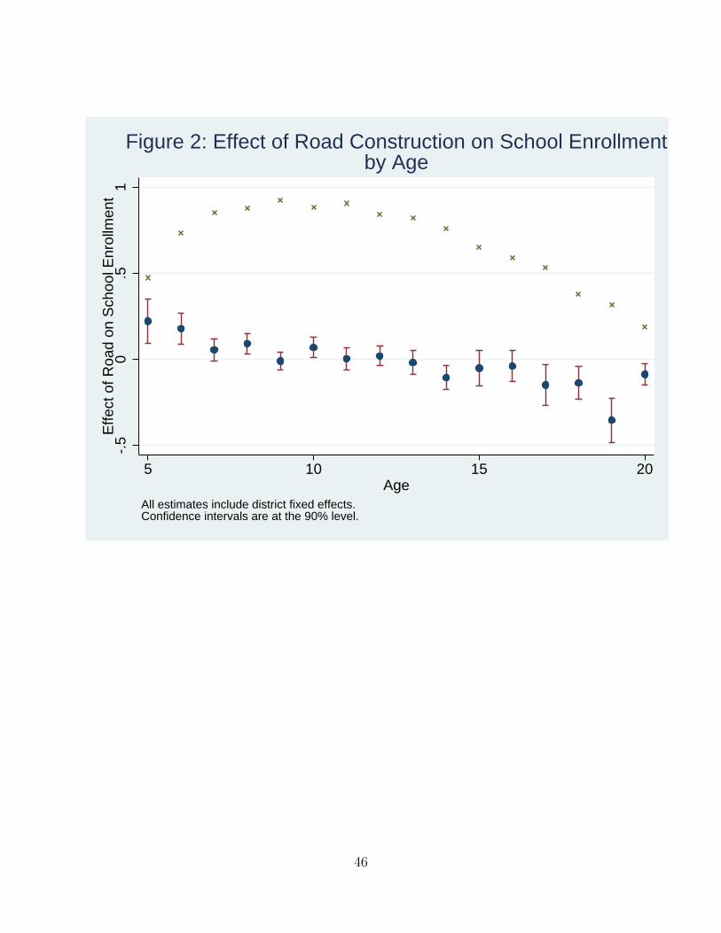
-.5

0.5

1E

ffect

of R

oad

on S

choo

l Enr

ollm

ent

5 10 15 20Age

All estimates include district fixed effects.Confidence intervals are at the 90% level.

Figure 2: Effect of Road Construction on School Enrollmentby Age

46

-.1

0.1

.2.3

.4E

ffect

of R

oad

on E

mpl

oym

ent

14 16 18 20Age

All estimates include district fixed effects.Confidence intervals are at the 90% level.

Figure 3: Effect of Road Construction on Employmentby Age

47

Coefficient Std. Error Baseline Mean

500 > p > 1000 0.261*** (0.03)

p > 1000 0.415*** (0.06)

Population 0.595 (0.47) 625.70

SC Population 0.004 (0.01) 0.37

Distance from Town -0.158 (0.17) 25.29

Panchayat HQ 0.080*** (0.02) 0.08

Primary School 0.036** (0.01) 0.79

High School -0.016 (0.01) 0.03

Adult Literacy Center 0.007 (0.01) 0.08

Primary Health Center -0.013 (0.01) 0.03

Commercial Bank -0.017 (0.01) 0.05

Post Office -0.005 (0.01) 0.23

Telephone -0.004 (0.01) 0.26

Power Supply 0.002 (0.01) 0.71

R-squared 0.216

Standard errors in parentheses, clustered by state

***, **, * indicate significance at 1, 5 and 10%

Sample of 272,412 villages. Includes state fixed effects

Table 1: Likelihood of Road Construction by Endline

48

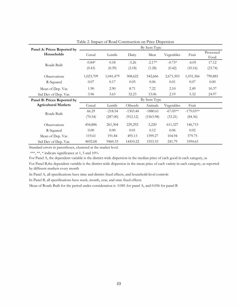
Cereal Lentils Dairy Meat Vegetables FruitProcessed

Food

-0.84* 0.18 -3.26 -2.17* -0.73* -6.05 17.12

(0.43) (0.39) (2.18) (1.28) (0.42) (10.16) (23.74)

1,023,709 1,041,479 308,622 542,666 2,671,503 1,031,366 790,881

0.07 0.17 0.05 0.06 0.01 0.07 0.00

1.90 2.90 8.71 7.22 2.10 2.49 10.37

3.96 3.63 32.23 13.06 2.19 5.32 24.97

Cereal Lentils Oilseeds Animals Vegetables Fruit

66.29 -218.54 -1303.44 -1880.61 -67.05** -179.03**

(70.54) (287.00) (912.12) (1563.98) (33.21) (84.36)

454,886 261,304 229,292 5,220 611,327 146,715

0.00 0.00 0.01 0.12 0.06 0.02

119.61 191.84 495.13 1399.27 104.94 379.75

4692.68 9460.33 14410.22 1553.33 241.79 3394.63

Standard errors in parentheses, clustered at the market level.

***, **, * indicate significance at 1, 5 and 10%

In Panel A, all specifications have time and district fixed effects, and household-level controls

In Panel B, all specifications have week, month, year, and state fixed effects

Mean of Roads Built for the period under consideration is 0.081 for panel A, and 0.056 for panel B

Table 2. Impact of Road Construction on Price Dispersion

Roads Built

Observations

R-Squared

Std Dev of Dep. Var.

By Item TypePanel A: Prices Reported by

Households

Panel B: Prices Reported by

Agricultural Markets

By Item Type

Mean of Dep. Var.

For Panel A, the dependent variable is the district-wide dispersion in the median price of each good in each category, as

reported by households in each villageFor Panel B,the dependent variable is the district-wide dispersion in the mean price of each variety in each category, as reported

by different markets every month

Roads Built

Observations

R-Squared

Mean of Dep. Var.

Std Dev of Dep. Var.

49

12

34

56

78

910

0.04

0.04

0.05*

0.05*

0.03

0.03

0.06*

0.05*

0.05*

0.05*

(0.03)

(0.03)

(0.03)

(0.03)

(0.031)

(0.031)

(0.031)

(0.027)

(0.027)

(0.029)

0.06**

0.06**

0.05*

0.05*

0.06**

*0.06**

*

(0.02)

(0.02)

(0.029)

(0.029)

(0.022)

(0.021)

322,625

322,625

322,625

322,625

151,687

151,687

151,687

170,938

170,938

170,938

0.039

0.049

0.007

0.017

0.051

0.063

0.021

0.032

0.041

0.013

0.8

0.8

0.8

0.8

0.77

0.77

0.77

0.83

0.83

0.83

-0.09**

-0.08*

-0.12**

*-0.11**

-0.09*

-0.09*

-0.09*

-0.08*

-0.08*

-0.11**

(0.04)

(0.04)

(0.04)

(0.04)

(0.046)

(0.044)

(0.048)

(0.045)

(0.044)

(0.044)

0.00

0.00

0.01

0.00

0.00

0.00

(0.03)

(0.03)

(0.034)

(0.034)

(0.031)

(0.03)

242,761

242,761

242,761

242,761

112,890

112,890

112,890

129,871

129,871

129,871

0.056

0.085

0.011

0.046

0.077

0.105

0.042

0.051

0.085

0.046

0.46

0.53

0.46

0.46

0.37

0.37

0.37

0.53

0.53

0.53

NY

NY

NY

YN

YY

NN

YY

NN

YN

NY

YY

NN

YY

NY

YN

Standard errors in paren

theses, clustered

at the district level

***, **, * indicate sign

ifican

ce at 1, 5 and 10%

All sp

ecifications hav

e time fixe

d effec

ts

Mean of Road

s Built: 0.052

The dep

enden

t variable is an

indicator for whether the resp

onden

t reported

that the ch

ild's primary occ

upation w

as going to sch

ool

Tab

le 3. Im

pact of Road

Construction on Sch

ool Enro

llmen

t

Overall

Impacts by Gen

der

Girls

Boys

R-Squared

Baseline mean

Road

s Built

Pre-pro

gram

Road

s

State FE

Observations

R-Squared

Baseline mean

Panel A: Impact on 5-

14 year-olds

Panel A: Impact on 14-

20 year-olds

Pre-pro

gram

Road

s

Indiv C

ontrols

District FE

Road

s Built

Observations

50

12

34

56

78

910

0.10**

*0.09**

*0.11**

*0.10**

*0.11**

*0.10**

*0.09**

*0.10**

0.09**

0.12**

*

(0.04)

(0.03)

(0.03)

(0.06)

(0.036)

(0.035)

(0.033)

(0.045)

(0.038)

(0.04)

-0.01

0.13**

-0.02

-0.02

0.00

-0.02

(0.02)

(0.06)

(0.021)

(0.021)

(0.03)

(0.027)

0.43**

*-0.29**

-0.55**

*0.48**

*-0.06

-0.19

(0.029)

(0.115)

(0.113)

(0.035)

(0.135)

(0.135)

NY

NY

NY

YN

YY

NN

YY

NN

YN

NY

YY

NN

YY

NY

YN

216,225

216,225

216,225

216,225

103,993

103,993

103,993

112,232

112,232

112,232

0.057

0.22

0.006

0.172

0.092

0.16

0.078

0.058

0.244

0.206

0.24

0.24

0.24

0.24

0.15

0.15

0.15

0.31

0.31

0.31

12

34

56

78

0.12**

0.11**

0.09*

0.09

0.01

0.01

0.02

0.01

(0.054)

(0.054)

(0.06)

(0.057)

(0.01)

(0.009)

(0.01)

(0.011)

-0.12**

*-0.12**

*-0.02**

*-0.02**

*

(0.038)

(0.037)

(0.006)

(0.006)

NY

NY

NY

NY

NN

YY

NN

YY

YY

NN

YY

NN

187,597

187,597

187,597

187,597

186,412

186,412

186,412

186,412

0.137

0.222

0.004

0.103

0.014

0.049

0.001

0.036

0.41

0.41

0.41

0.41

0.96

0.96

0.95

0.96

Standard errors in paren

theses, clustered

at the district level

***, **, * indicate sign

ifican

ce at 1, 5 and 10%

All specifications hav

e time fixed

effects

Mean of Road

s Built: 0.052

Tab

le 4. Im

pact of Road

Construction on E

mploym

ent

District FE

Overall

Impacts by Gen

der

Road

s Built

Boys

Girls

Panel A: Impact on 14-20

year-olds

Pre-pro

gram

Road

s

Constan

t

Indiv C

ontrols

State FE

Observations

R-Squared

Baseline mean

Impacts by Gen

der

Women

Men

Road

s Built

State FE

Observations

R-Squared

Baseline mean

Panel B: Impact on Prime-

Age Individuals

Pre-pro

gram

Road

s

Indiv C

ontrols

District FE

51

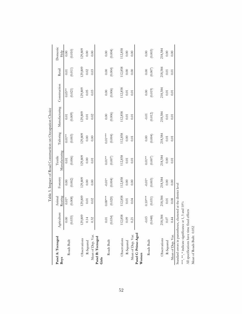
Agr

iculture

Anim

al

Rea

ring

Fore

stry

Tex

tile

Man

ufa

cturing

Tai

loring

Man

ufa

cturing

Const

ruct

ion

Ret

ail

Dom

estic

Hel

p

0.0

00.0

1*

0.0

00.0

10.0

1**

0.0

10.0

5**

0.0

10.0

0

(0.0

35)

(0.0

08)

(0.0

02)

(0.0

06)

(0.0

03)

(0.0

09)

(0.0

21)

(0.0

11)

(0.0

10)

129,8

09

129,8

09

129,8

09

129,8

09

129,8

09

129,8

09

129,8

09

129,8

09

129,8

09

0.1

40.0

10.0

00.0

00.0

00.0

10.0

50.0

20.0

0

0.3

20.0

20.0

00.0

10.0

00.0

20.0

30.0

30.0

0

0.0

10.0

8**

*-0

.01*

0.0

1**

0.0

1**

*0.0

00.0

00.0

00.0

0

(0.0

34)

(0.0

20)

(0.0

04)

(0.0

07)

(0.0

04)

(0.0

06)

(0.0

06)

(0.0

04)

(0.0

04)

112,8

58

112,8

58

112,8

58

112,8

58

112,8

58

112,8

58

112,8

58

112,8

58

112,8

58

0.0

90.0

10.0

00.0

10.0

00.0

10.0

10.0

00.0

0

0.2

10.0

40.0

00.0

10.0

10.0

10.0

10.0

00.0

0

-0.0

30.1

0**

*-0

.01*

0.0

1**

0.0

0-0

.01

0.0

00.0

00.0

0

(0.0

48)

(0.0

31)

(0.0

03)

(0.0

07)

(0.0

04)

(0.0

12)

(0.0

19)

(0.0

07)

(0.0

03)

218,5

84

218,5

84

218,5

84

218,5

84

218,5

84

218,5

84

218,5

84

218,5

84

218,5

84

0.0

70.0

10.0

00.0

00.0

10.0

10.0

10.0

10.0

0

0.4

40.0

80.0

00.0

10.0

10.0

10.0

10.0

10.0

0

Sta

ndar

d e

rrors

in p

aren

thes

es, cl

ust

ered

at th

e dis

tric

t le

vel

***,

**,

* indic

ate

sign

ific

ance

at 1, 5 a

nd 1

0%

All

spec

ific

atio

ns

hav

e tim

e fixe

d e

ffec

ts

Mea

n o

f R

oad

s B

uilt

: 0

.052

Mea

n o

f D

ep. V

ar.

Panel A: Teenaged

Boys

Tab

le 5

. Im

pac

t of R

oad

Const

ruct

ion o

n O

ccupat

ion C

hoic

e

Road

s B

uilt

Obse

rvat

ions

R-S

quar

ed

Obse

rvat

ions

R-S

quar

ed

Mea

n o

f D

ep. V

ar.

Panel B: Teenaged

Girls

Panel C: Prime-Aged

WomenRoad

s B

uilt

Obse

rvat

ions

R-S

quar

ed

Mea

n o

f D

ep. V

ar.

Road

s B

uilt

52

All Crops Cash Crops Food Crops

Area under Fertilizer

-43.17 1,583.61*** -678.47

(391.82) (605.78) (555.69)

10,266.18*** -2,162.47 17,944.83***

(2524.90) (2467.75) (3990.16)

Baseline Mean 22,281.36 7,901.07 13,936.63

Baseline Std. Dev 76,771.20 32,036.28 44,764.57

Area under Hybrid Seeds

692.33 1,572.23*** 282.12

(463.56) (581.45) (675.55)

6,056.85** -2,709.28 13,067.63***

(2372.22) (2266.51) (3740.42)

Baseline Mean 20,187.12 6,670.74 12,905.33

Baseline Std. Dev 76,794.03 27,471.54 46,340.40

N 19,087 6,666 12,421

Clustered standard errors in parentheses. ***, **, * indicate significance at 1, 5 and 10%

Includes district fixed effects and district-level covariates

Mean of roads built over the analysis period is 0.068

Post * Roads Built

Post-period Dummy

Post * Roads Built

Post-period Dummy

Table 6. Impact of Road Construction on Technology Adoption in Agriculture, 2001-2007

53

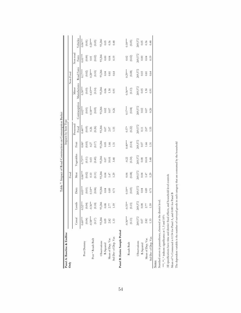
Cer

eal

Len

tils

Dai

ryM

eat

Veg

etab

les

Fru

itP

roce

ssed

Fo

od

Co

ntr

acep

tiv

es

Min

or

Man

ufa

ctu

res

Ro

ad F

ares

No

n-r

oad

Far

esV

ehic

les

0.6

0**

*0

.52

***

0.0

5**

*0

.06

***

0.7

5**

*0

.06

*0

.44

***

0.0

2**

*0

.30

***

0.1

7**

*0

.01

***

0.0

6**

*

(0.0

4)

(0.0

4)

(0.0

1)

(0.0

2)

(0.1

1)

(0.0

3)

(0.0

5)

(0.0

1)

(0.0

3)

(0.0

2)

(0.0

0)

(0.0

1)

-0.5

8**

*-0

.36

**0

.14

**0

.10

0.0

30

.27

0.2

60

.18

***

0.4

3**

*0

.28

***

0.0

10

.20

***

(0.1

7)

(0.1

8)

(0.0

6)

(0.1

1)

(0.4

5)

(0.1

7)

(0.2

6)

(0.0

5)

(0.1

4)

(0.1

0)

(0.0

2)

(0.0

5)

93

,26

69

3,2

66

93

,26

69

3,2

66

93

,26

69

3,2

66

93

,26

69

3,2

66

93

,26

69

3,2

66

93

,26

69

3,2

66

0.0

90

.08

0.0

40

.04

0.0

70

.05

0.0

70

.02

0.0

60

.04

0.0

00

.05

2.8

22

.77

0.8

91

.47

10

.01

1.6

62

.07

0.0

71

.30

0.8

10

.04

0.3

6

1.3

31

.59

0.7

11

.29

3.4

81

.31

1.5

50

.26

0.9

10

.64

0.1

90

.48

-0.3

6**

*-0

.35

**0

.10

**0

.04

-0.2

20

.40

***

0.3

7*

0.1

7**

*0

.36

***

0.2

9**

*0

.02

0.1

8**

*

(0.1

3)

(0.1

5)

(0.0

5)

(0.0

8)

(0.3

4)

(0.1

4)

(0.2

2)

(0.0

4)

(0.1

3)

(0.0

8)

(0.0

2)

(0.0

5)

26

9,5

72

26

9,5

72

26

9,5

72

26

9,5

72

26

9,5

72

26

9,5

72

26

9,5

72

26

9,5

72

26

9,5

72

26

9,5

72

26

9,5

72

26

9,5

72

0.0

70

.08

0.0

40

.04

0.0

80

.07

0.1

10

.02

0.0

50

.03

0.0

00

.05

2.8

22

.77

0.8

91

.47

10

.01

1.6

62

.07

0.0

71

.30

0.8

10

.04

0.3

6

1.3

31

.59

0.7

11

.29

3.4

81

.31

1.5

50

.26

0.9

10

.64

0.1

90

.48

No

tes:

Sta

nd

ard

err

ors

in

par

enth

eses

, cl

ust

ered

at

the

dis

tric

t le

vel

.

***

, **

, *

ind

icat

e si

gnif

ican

ce a

t 1

, 5

an

d 1

0%

All

sp

ecif

icat

ion

s h

ave

tim

e an

d d

istr

ict

fix

ed e

ffec

ts,

and

ho

use

ho

ld-l

evel

co

ntr

ols

Mea

n o

f %

Co

nn

ecte

d i

s 0

.15

4 f

or

Pan

el A

, an

d 0

.08

1 f

or

Pan

el B

Th

e d

epen

den

t v

aria

ble

is

the

nu

mb

er o

f su

rvey

ed g

oo

ds

in e

ach

cat

ego

ry t

hat

are

co

nsu

med

by

the

ho

use

ho

ld

R-S

qu

ared

Mea

n o

f D

ep.

Var

.

Std

Dev

of

Dep

. V

ar.

Ob

serv

atio

ns

Mea

n o

f D

ep.

Var

.

Std

Dev

of

Dep

. V

ar.

Panel B: Entire Sample Period

Ro

ads

Bu

ilt

Po

st D

um

my

Po

st *

Ro

ads

Bu

ilt

Ob

serv

atio

ns

R-S

qu

ared

Tab

le 7

. Im

pac

t o

f R

oad

Co

nst

ruct

ion

on

Co

nsu

mp

tio

n B

ask

et

Panel A: Baseline & Endline

Only

Imp

acts

by

Item

Typ

e

Fo

od

No

n-F

oo

d

54

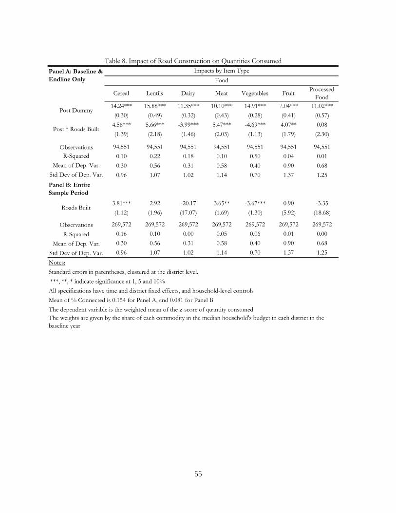
Cereal Lentils Dairy Meat Vegetables FruitProcessed

Food

14.24*** 15.88*** 11.35*** 10.10*** 14.91*** 7.04*** 11.02***

(0.30) (0.49) (0.32) (0.43) (0.28) (0.41) (0.57)

4.56*** 5.66*** -3.99*** 5.47*** -4.69*** 4.07** 0.08

(1.39) (2.18) (1.46) (2.03) (1.13) (1.79) (2.30)

94,551 94,551 94,551 94,551 94,551 94,551 94,551

0.10 0.22 0.18 0.10 0.50 0.04 0.01

0.30 0.56 0.31 0.58 0.40 0.90 0.68

0.96 1.07 1.02 1.14 0.70 1.37 1.25

3.81*** 2.92 -20.17 3.65** -3.67*** 0.90 -3.35

(1.12) (1.96) (17.07) (1.69) (1.30) (5.92) (18.68)

269,572 269,572 269,572 269,572 269,572 269,572 269,572

0.16 0.10 0.00 0.05 0.06 0.01 0.00

0.30 0.56 0.31 0.58 0.40 0.90 0.68

0.96 1.07 1.02 1.14 0.70 1.37 1.25

Notes:

Standard errors in parentheses, clustered at the district level.

***, **, * indicate significance at 1, 5 and 10%

All specifications have time and district fixed effects, and household-level controls

Mean of % Connected is 0.154 for Panel A, and 0.081 for Panel B

The dependent variable is the weighted mean of the z-score of quantity consumed

Roads Built

Observations

R-Squared

The weights are given by the share of each commodity in the median household's budget in each district in the

baseline year

Mean of Dep. Var.

Std Dev of Dep. Var.

Panel A: Baseline &

Endline Only Food

Table 8. Impact of Road Construction on Quantities Consumed

Impacts by Item Type

Post Dummy

Post * Roads Built

Observations

R-Squared

Mean of Dep. Var.

Std Dev of Dep. Var.

Panel B: Entire

Sample Period

55

5-14 14-20 14-20 Adult Men Adult Women

Post Dummy 0.03*** 0.03** -0.05*** -0.01 -0.02

(0.01) (0.01) (0.01) (0.00) (0.02)

Post * Roads Built -0.04 -0.07 0.06 0 0.08

(0.05) (0.06) (0.07) (0.02) (0.07)

Observations 145,440 88,325 46,213 74,607 75,373

R-Squared 0.01 0.00 0.01 0.01 0.02

Baseline mean 0.69 0.36 0.39 0.95 0.47

Notes:

Standard errors in parentheses, clustered at the district level.

***, **, * indicate significance at 1, 5 and 10%

All specifications have time and district fixed effects, and household-level controls

Enrollment Employment

Table 9: Placebo Test - Program Roads on 1993-1999 Outcomes

56

Cereal

Lentils

Dairy

Meat

Vegetables

Fruit

Processed

Food

Contraception

Minor

Manufactures

Road Fares

Non-road

Fares

Vehicles

0.47***

0.23***

0.05***

-0.59***

1.15***

0.30***

0.26***

0.00

0.04

-0.01

0.01**

0.04***

(0.04)

(0.04)

(0.01)

(0.03)

(0.10)

(0.03)

(0.03)

(0.01)

(0.03)

(0.01)

(0.01)

(0.01)

-0.12

-0.07

0.05

0.14

1.40***

0.10

-0.17

-0.04

-0.21

0.02

-0.02

-0.02

(0.18)

(0.16)

(0.05)

(0.15)

(0.43)

(0.14)

(0.12)

(0.04)

(0.15)

(0.08)

(0.01)

(0.04)

95,134

95,134

95,134

95,134

95,134

95,134

95,134

95,134

95,134

95,134

95,134

95,134

0.04

0.02

0.04

0.06

0.07

0.04

0.03

0.00

0.01

0.01

0.00

0.00

2.43

2.51

0.81

1.95

8.45

1.28

0.65

0.08

1.28

0.78

0.03

0.34

Notes:

Standard errors in parentheses, clustered at the district level.

***, **, * indicate sign

ificance at 1, 5 and 10%

All specifications have time and district fixed effects, and household-level controls

The dependent variable is the number of surveyed goods in each category that are consumed by the household

Table 10: Placebo Test - Program

Roads on 1993-1999 O

utcomes

Impacts by Item

Type

Food

Non-Food

Mean of Dep. Var.

Post D

ummy

Post * Roads Built

Observations

R-Squared

57

Table 11: Placebo Test - Effect of Roads Built in Future on Current Outcomes

5-14 14-20 14-20 Adult Men Adult Women

Roads Built by:

t -0.04 -0.17 0.29*** -0.02 0.21

(0.12) (0.14) (0.11) (0.04) (0.21)

t+1 0.07 0.01 -0.06 -0.01 -0.06

(0.14) (0.12) (0.09) (0.05) (0.15)

t+2 -0.11 -0.02 -0.15 0.05 0.1

(0.10) (0.12) (0.10) (0.05) (0.15)

Observations 130,713 100,420 45,838 75,796 72,120

R-Squared 0.013 0.032 0.335 0.053 0.076

Baseline mean 0.8 0.46 0.24 0.95 0.41

Joint p-value 0.55 0.99 0.24 0.53 0.78

Notes:

Standard errors in parentheses, clustered at the district level.

***, **, * indicate significance at 1, 5 and 10%

All specifications have time and district fixed effects, and household-level controls

Enrollment Employment

58

14-20 Boys 14-20 Girls Prime-Age Men Prime-Age Women

0.02*** 0.03* 0.00 0.03*** 0.02*

(0.007) (0.014) (0.021) (0.008) (0.008)

0.13*** 0.12 0.36** 0.14*** 0.01

(0.038) (0.080) (0.179) (0.045) (0.062)

Observations 134,860 9,787 3,106 50,853 13,271

R-Squared 0.01 0.01 0.02 0.01 0.00

Mean of Dep. Var. 0.13 0.16 0.07 0.16 0.06

Standard errors in parentheses, clustered at the district level.

***, **, * indicate significance at 1, 5 and 10%

All specifications have time and district fixed effects, and household-level controls

Table 12: Impact of Road Construction on Employment Location (location dummy = 1 for urban, 0 for rural)

OverallImpacts by Group

Post Dummy

Post * Roads Built

59

12

34

56

78

-0.08

-0.07

-0.03

-0.04

0.01

0.00

0.01

0.00

(0.09)

(0.08)

(0.07)

(0.06)

(0.01)

(0.03)

(0.03)

(0.03)

0.12**

0.13**

0.07**

*0.06**

*

(0.05)

(0.06)

(0.02)

(0.02)

NY

NY

NY

NY

NN

YY

NN

YY

YY

NN

YY

NN

162,840

162,840

162,956

162,840

434,642

434,642

435,045

434,642

0.18

0.24

0.00

0.04

0.14

0.17

0.01

0.13

0.50

0.50

0.51

0.51

0.50

0.50

0.45

0.45

Standard errors in paren

theses, clustered

at the district level

***, **, * indicate sign

ifican

ce at 1, 5 and 10%

All specifications hav

e time fixed

effects

Mean of Road

s Built: 0.052

Observations

R-Squared

Baseline mean

Pre-pro

gram

Road

s

Indiv C

ontrols

District FE

State FE

Impacts by Gen

der

Women

Men

Road

s Built

Tab

le 13. Im

pact of Road

Construction on W

age Employm

ent

60

Size of Household

-0.08

(0.115)

269,572

0.01

4.83

2.48

Standard errors in parentheses, clustered at the district level.

***, **, * indicate significance at 1, 5 and 10%

All specifications have time and district fixed effects, and household-level controls

Mean of Roads Built: 0.081

Std Dev of Dep. Var.

Table 14. Impact of Program Intensity on Household Size

Roads Built

Observations

R-Squared

Mean of Dep. Var.

61

Appendix

A.1 CDF of Connectivity

0

.2

.4

.6

.8

1

Cum

ulat

ive

Pro

babi

lity

of h

avin

g a

road

0 5 10 15Years since Program Inception

p < 250 250 < p < 500500 < p < 1000 p > 1000

• 12 years since program inception corresponds to being unconnected at the time this

data was collected.

• This graph is based on all-India data, and does not account for state-wise differences

in program implementation.

62

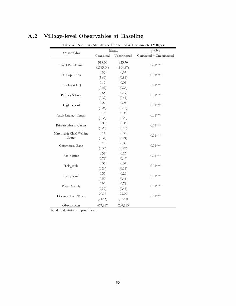
A.2 Village-level Observables at Baseline

p value

Connected Unconnected Connected = Unconnected

929.20 625.70

(2345.04) (864.47)

0.32 0.37

(3.69) (0.81)

0.19 0.08

(0.39) (0.27)

0.88 0.79

(0.32) (0.41)

0.07 0.03

(0.26) (0.17)

0.16 0.08

(0.36) (0.28)

0.09 0.03

(0.29) (0.18)

0.11 0.06

(0.31) (0.24)

0.13 0.05

(0.33) (0.22)

0.52 0.23

(0.71) (0.49)

0.05 0.01

(0.24) (0.11)

0.53 0.26

(0.50) (0.44)

0.90 0.71

(0.30) (0.46)

20.78 25.29

(21.45) (27.31)

Observations 477,917 280,210

0.01***

0.01***Distance from Town

0.01***

0.01***

0.01***

0.01***

0.01***

0.01***

0.01***

0.01***

0.01***

Maternal & Child Welfare

Center

Commercial Bank

Post Office

Telegraph

Standard deviations in parentheses.

Telephone

ObservablesMeans

Table A1: Summary Statistics of Connected & Unconnected Villages

Power Supply

Primary School

Total Population

SC Population

Panchayat HQ

High School

Adult Literacy Center

Primary Health Center

0.01***

0.01***

0.01***

63

A.3 First Stage Effects of Population Category on Percent Con-

nected

% Connected during program

Population

250 - 500 0.26

(0.161)

500 - 1000 0.31***

(0.063)

> 1000 0.26***

(0.054)

Pre-Program Connectivity -0.04

(0.06)

Observations 241,565

R-Squared 0.06

F-stat 11.56

P-Value 0

***, **, * indicate significance at 1, 5 and 10%

Includes state fixed effects.

Standard errors in parentheses, clustered at state level

Table A1: First Stage of Instrumenting Connectivity on Eligibility

64

A.4 IV Estimates

Ce

rea

lL

en

tils

Da

iry

Me

at

Ve

ge

tab

les

Fru

itP

roce

sse

d

Fo

od

Aw

are

ne

ss

Go

od

s

Min

or

Ma

nu

fact

ure

sR

oa

d F

are

sN

on

-ro

ad

Fa

res

Ve

hic

les

-0.0

40

.25

0.2

4*

0.2

40

.31

*0

.18

*0

.33

*0

.18

0.0

60

.52

***

0.0

30

.78

**

(0.0

8)

(0.2

3)

(0.1

3)

(0.2

0)

(0.1

9)

(0.1

0)

(0.1

9)

(0.1

5)

(0.1

3)

(0.1

9)

(0.0

5)

(0.3

1)

-0.0

20

.06

0.0

8**

*0

.04

0.0

7*

0.0

5**

*0

.07

*0

.01

0.0

10

.13

***

-0.0

10

.16

**

(0.0

2)

(0.0

5)

(0.0

3)

(0.0

4)

(0.0

4)

(0.0

2)

(0.0

4)

(0.0

3)

(0.0

3)

(0.0

3)

(0.0

1)

(0.0

6)

0.3

00

.32

0.2

20

.47

0.1

70

.14

0.1

20

.10

0.1

30

.11

0.0

40

.18

0.1

30

.21

0.1

50

.21

0.3

30

.10

0.1

40

.04

0.0

90

.20

0.0

10

.18

0.0

60

.12

0.1

20

.18

0.1

20

.08

0.1

00

.13

0.0

60

.16

0.0

60

.24

Sta

nd

ard

err

ors

in

pa

ren

the

ses,

clu

ste

red

at

the

dis

tric

t le

ve

l.

***

, **,

* i

nd

ica

te s

ign

ific

an

ce a

t 1

, 5 a

nd

10

%

All

sp

eci

fica

tio

ns

ha

ve

tim

e a

nd

sta

te f

ixe

d e

ffe

cts,

an

d d

istr

ict-

lev

el

con

tro

ls

Sa

mp

le c

on

tain

s 2

65

,38

2 h

ou

seh

old

s

Me

an

of

% C

on

ne

cte

d P

ost

-Pro

gra

m:

0.0

81

Fo

od

Ta

ble

A2

. Im

pa

ct o

f P

rog

ram

In

ten

sity

on

Co

nsu

mp

tio

n B

ask

et

(IV

)

Imp

act

s b

y I

tem

Ty

pe

No

n-F

oo

d

R-S

qu

are

d

Me

an

of

De

p. V

ar.

Std

De

v o

f D

ep

. Va

r.

% C

on

ne

cte

d b

y

Pro

gra

m

Pre

-Pro

gra

m

Co

nn

ect

ivit

y

65

A.5 Consumption during Monsoon

Cereal Lentils Dairy Meat Vegetables FruitProcessed

Food

0.00 0.00 0.00 -0.01*** -0.01*** -0.01*** 0.00

(0.01) (0.01) (0.01) (0.01) (0.01) (0.01) (0.01)

0.01 0.01 0.01* 0.04*** 0.02* 0.04*** 0.02*

(0.01) (0.01) (0.01) (0.01) (0.01) (0.01) (0.01)

-0.01 -0.03** 0.02* -0.01 -0.02 0.02** 0.03*

(0.01) (0.01) (0.01) (0.01) (0.01) (0.01) (0.02)

232,772 232,772 232,772 232,772 232,772 232,772 232,772

0.07 0.07 0.04 0.04 0.07 0.07 0.10

0.14 0.22 0.15 0.20 0.34 0.10 0.14

Standard errors in parentheses, clustered at the district level.

***, **, * indicate significance at 1, 5 and 10%

All specifications have time and district fixed effects, and household-level controls

Mean of % Connected Post-Program: 0.081

Mean of Dep. Var.

Table A3. Impact on Consumption Basket during Monsoon

Monsoon Dummy

Roads Built *

Monsoon Dummy

Roads Built

Observations

R-Squared

66

The Bargaining Power of Missing Women:Evidence from a Sanitation Campaign in India

Yaniv Stopnitzky∗

NOVEMBER 15, 2013

Abstract

Female bargaining power in rural Haryana, as in much of northern India, is con-

strained by widespread discrimination against women. In recent years, however, women

successfully demand private sanitation facilities from potential husbands as a precondi-

tion for marriage. I study this manifestation of bargaining power by modeling latrine

adoption as an investment that males can make to improve their desirability on the mar-

riage market, and I show that increasing proportions of females with strong sanitation

preferences drive male investment in toilets. Moreover, I demonstrate women’s ability to

secure latrines increases when they are relatively scarce in a marriage market. I test these

predictions empirically by studying a sanitation program in Haryana, India, known col-

loquially as “No Toilet, No Bride”. Using a triple difference empirical strategy based on

households with and without marriageable boys, in Haryana and comparison states, be-

fore and after program exposure, I provide evidence that male investment in sanitation

increased by 15% due to the program. Further, the program effect is four times larger

in marriage markets where women are scarce (26%) as compared to marriage markets

where women are abundant (6%). These results suggest the relative scarcity of women

in Haryana has, conditional on women surviving to marriageable age, improved the

ability of the remaining women to secure valuable goods.

JEL Classification: D1, J12, O12, O13

∗Affiliation: University of San Francisco. Email: ystopnitzky@usfca.edu. I am grateful to Dean Kar-lan, Matthew Kotchen, Sheila Olmstead, and Chris Udry for their guidance and support. I also thank DougGollin, Mark Rosenzweig, Paul Schultz, Mushfiq Mobarak, Paul Gertler, Sebastian Galiani, Dan Keniston, JackMolyneaux, Alexandra Orsola-Vidal, Sumeet Patil, Treb Allen, Melanie Morten, Camilo Dominguez, Snaeb-jorn Gunnsteinsonn, Namrata Kala, Rahul Deb, Gharad Bryan, and seminar participants at Yale, Columbia,Arizona State, Resources for the Future, University of San Francisco, Universitat Pompeu Fabra, Tel Aviv Uni-versity, Hebrew University, and the AERE Summer Conference for discussion and numerous comments.

1

1 Introduction

Women in rural Haryana suffer from discrimination that is widespread and strong enoughto generate the most skewed state-level sex ratio in all of India.1 Due to parental preferencesfor sons over daughters, parents provide differential post-natal care to boys and girls (DasGupta (1987)), invest preferentially in male fetuses (Bharadwaj & Nelson (2010)), and/orselectively abort female fetuses (Arnold et al. (2002), Qian (2008)). Each of these factorsexacerbates the sex imbalance. Further, if women survive to adulthood, they face numer-ous gender-specific constraints on their ability to travel or work outside of the household(Eswaran et al. (2009)).

In this social context of discrimination, females in rural Haryana have in recent yearsdemanded from men and obtained a particularly valuable good—toilets—as a preconditionfor marriage. Women value toilets to a greater extent than males because they suffer dis-proportionately from male staring and harassment when they defecate, urinate, or attend tomenstrual hygiene in public places. For this reason, private latrines generate benefits thatare disproportionately enjoyed by females. The change that has allowed women to success-fully demand latrines in marriage negotiations is associated with an unusual sanitation cam-paign commonly known as “No Toilet, No Bride", which Haryana state authorities initiatedin 2005. The campaign encouraged families of marriage-age girls to demand that potentialsuitors’ families construct a latrine prior to marriage. Mass media messaging via billboards,posters, and radio advertisements emphasized phrases such as “no toilet, no bride” and “noloo, no I do”. These messages were framed by women’s concerns about privacy and dig-nity when they defecate in the open, a behavior that is routine among roughly 70% of ruralhouseholds in Haryana in 2004. Although the rationale for public investment in sanitationprograms is the reduction of fecal pollution and the morbidity associated with widespreadopen defecation, the emphasis of “No Toilet, No Bride”, combined with the fact that privatebenefits accrue largely to women, provides a unique opportunity to study female bargainingpower under widespread discimination.

The “No Toilet, No Bride" program serves as a source of exogenous variation that altersthe distribution of female preferences for sanitation. Because women move into the houseof their husbands or their husbands’ families at the time of marriage, the program’s focuson women’s preferences indirectly targets male behavior. I study the male response to theprogram by modeling latrine adoption in a transferable utility model of the marriage mar-ket. In the model, men can choose to invest in sanitation in order to raise their returns frommarriage, which also depend on marriage market conditions. The model generates two key

1Source: Indian Census, 2011. Note that two non-state union territories, Chandigarh and Delhi, both adja-cent to Haryana, have slightly worse sex ratios.

2

empirical predictions. First, I show that increasing the proportion of women with strongpreferences for sanitation will cause men to increase their investments in latrines. Second, Iextend the model to focus on the role of sex ratios, and I demonstrate the marriage marketreturn to male investment increases to a greater extent when females are relatively scarceas compared to when females are abundant. Finally, I analyze the potential role of dowriesin altering these empirical predictions, and I establish that the model’s predictions on maleinvestment will remain unchanged because dowry is determined in equilibrium as one com-ponent of the marital surplus.

I test these predictions using two rounds of the District-Level Household and FacilitySurvey (2004, 2008/9), a nationally representative, household data set. I employ an empir-ical strategy based on the intuition that the “No Toilet, No Bride” campaign exerts dispro-portionate pressure to adopt a latrine on those households with boys active on the marriagemarket. If the program was successful in linking sanitation with the marriage market, thenhouseholds with boys of marriageable age face exogenous pressure to build a latrine, andthey should therefore have a higher probability of latrine ownership after exposure to theprogram. Because such households could differ from households without marriageable ageboys in a variety of unobserved ways, my econometric specification controls explicitly forthese unobserved characteristics. I implement a difference-in-difference-in-difference ap-proach that compares latrine ownership in households with and without boys of marriage-able age, in Haryana and comparison states from northern India, before the program startedand three to four years after the program began.

I find an increase of 4.3 percentage points (a 15% increase from a base of 28%) in thelatrine ownership differential between households with and without marriage-age boys inHaryana over the period 2004 to 2008 relative to the difference between latrine ownershiphouseholds with and without marriageable boys in comparison states. In addition, I providestrong, complementary evidence that latrine adoption is driven by whether households havemarriageable boys active in a highly competitive marriage market, i.e. one with an under-supply of women due to highly skewed sex ratios. Specifically, I find that Haryana’s ob-served latrine adoption due to “No Toilet, No Bride” is driven largely by marriage marketswith a scarcity of women; in these markets I estimate a program effect of 26% over baseline.In marriage markets without this scarcity, however, the “No Toilet, No Bride” treatmenteffect is one-fourth as large.

These results are robust to competing hypotheses that the program caused changes inmale preferences or increased latrine ownership by changing female preferences outside ofmarriage market channels. Evidence against the former hypothesis comes from a test ofprogram effects among households with boys slightly older than marriage age, and whowere thus too old to be affected by the program when they were active on the marriage

3

market. Similarly, I present evidence against the latter alternative hypothesis by analyzingthe ability of strictly single marriage-age girls to demand and obtain latrines. Thus, theprogram appears to operate specifically through the channel of marriage market bargaining.

Finally, I seek evidence on shifts in the intrahousehold sharing rule due to the “NoToilet, No Bride” program. Using a range of household assets and marriage-related vari-ables that women value, I find no evidence the program has caused women to substitutetoilets for other goods they value. On the contrary, women’s relative position appears tohave improved both in terms of age at marriage and the educational quality of their malespouses, while males appear to have been compensated in the form of motorbikes, perhapsin compensation for their sanitation expenditures. I am unable to determine empirically theintrahousehold allocation due to unobservables, but these results provide suggestive evi-dence that although “No Toilet, No Bride” has altered marital negotiations in various ways,women’s status has not worsened along multiple observable dimensions.

Consistent with theoretical predictions from a transferable utility marriage market modelwith endogenous investment in quality, these findings suggest that (i) the “No Toilet, NoBride” campaign has significantly increased latrine ownership by linking marriage match-ing to the acquisition of a good that females particularly value, and (ii) biased sex ratios haveincreased the relative bargaining power of women on the marriage market, thereby improv-ing their ability to demand goods. Thus, in an area with one of the most severely skewedsex ratios on earth, a local scarcity of women appears to have increased women’s bargainingpower, allowing them to obtain additional goods that they value.

This paper is organized as follows. Section 2 provides a social and economic backgroundto marriage markets in northern India and Haryana, specifically where the “No Toilet, NoBride” program operates. Section 3 presents a model of marriage matching with endoge-nous investments in quality; a fuller treatment can be found in the theoretical appendix.Section 4 discusses sanitation in rural India and important features of the “No Toilet, NoBride” program. Section 5 explains the empirical strategy, identification issues, and data.Section 6 contains the key empirical results. Robustness to competing hypotheses is dis-cussed in Section 6.3, and Section 7 discusses additional evidence on female bargaining andthe intrahousehold allocation. Section 8 concludes.

2 Marriage Markets in Northern India

Marriage markets in northern India are fundamentally shaped by social norms around pa-trilocality and caste endogamy. Moreover, the marriage negotiation process is structuredby the phenomena of arranged marriage and dowry. Marriages are typically arranged bythe parents of both families, often with the help of an intermediary matchmaker, who helps

4

identify suitors according to the criteria established by the families. The most important di-mensions along which potential spouses are valued include caste, religion, kinship, profes-sion, education, and physical attractiveness; the attractiveness of women is a characteristicparticularly important for men (Banerjee et al. (2009)). Together, these interlocking institu-tions play a primary role in shaping the opportunity sets faced by marriage-age individualsand in determining marital outcomes. In this section I provide an overview of these socialpractices and highlight those characteristics significant for the theory and empirics of thispaper.

2.1 Patrilocal Exogamy

The first important aspect of marriage in northern India, of which Haryana is a part, is thepractice of patrilocal/virilocal exogamy, i.e. the migration of newlywed brides out of theirhouseholds and into the residence of their husbands’ family located outside of the brides’home village (Gould (1961)). For example, data from the 1994 PGIRCS survey in the states ofUttar Pradesh and Karnataka suggest that 90% of imported brides originated from villageslocated within 67 kilometers of the sample villages (Bloch et al. (2004)). In their study of howvillage exogamy serves as a form of insurance against spatially correlated risks, Rosenzweig& Stark (1989) note that the average distance across which two rural Indian householdslinked through marriage was approximately 30 kilometers. These empirical findings arebroadly consistent with other qualitative evidence such as Dutt et al. (1981), which detailsmarriage-generated links for two Punjabi villages and finds that 80% of households had amarriage distance of 40 kilometers. Thus, although households practice strict village ex-ogamy (and appear to seek villages whose incomes do not covary strongly with the homevillage), households are typically searching for partners within a geographically definedarea. This descriptive fact is important for the purposes of this paper because later I adoptan empirical definition of marriage markets in reference to a household’s home district.2

2.2 Caste Endogamy

A second, crucial feature of Indian marriage matching is caste endogamy, i.e. the practice ofmarrying a spouse from within one’s own caste. For example, Banerjee et al. (2009) cite anopinion poll in which 74% of respondents from West Bengal define themselves as opposed tointer-caste marriage, and the authors note the practice of caste endogamy is so widespreadthat matrimonial classified advertisements, which are common in Indian newspapers, oftengroup listings by caste. In addition, these authors present evidence that individuals are will-

2The full definition I use is the intersection of caste, religion, marriage-age cohort, and district.

5

ing to trade substantial benefits in terms of spousal beauty, education, and/or wealth in or-der to marry within-caste. Later in the empirical section of this paper, I use such widespreadand strong preferences for caste endogamy, coupled with the pervasiveness of patrilocalexogamy described above, to justify my empirical definition of a marriage market.

2.3 Sex Ratios in Contemporary India

In India, particularly in the northern states, the phenomenon of “missing women”, i.e.women absent from the population due to skewed sex ratios, has a long history. For exam-ple, under British rule in the 19th century, census officials documented low ratios of womento men in northern India and British officials suspected the Rajputs, a large northern clan,of female infanticide (Chakraborty & Kim (2008)). Whereas in the past much of the ob-served sex imbalance was explained by such infanticide and/or differential neglect of girls(Das Gupta (1987)), the spread of ultrasound, amniocentesis, and doctor-provided abortiontechnology in recent decades has driven sex ratios among younger cohorts.3 Estimates us-ing data from the National Family Health Survey (NFHS-2, 1998/9) indicate that more than100,000 sex-selective abortions of female fetuses were being performed each year in India,many of them by private providers in contravention of (unenforced) government regulations(Arnold et al. (2002)).

The underlying driver of both differential neglect and selective abortion is a strong parentalpreference for sons. Parents prefer boys over girls for each birth order, but this effect in-creases dramatically for higher birth order children. In data from the District Level andHousehold Survey (DLHS 2008/9), 15% of married female respondents without children re-port wanting a boy but only 3% desire a girl, conditional on wanting another child. Forbirth orders higher than four, nearly 10 times more mothers state a preference for anotherson as compared to another girl (65% and 6%, respectively). Moreover, these patterns aredominated by preferences among households in northern Indian states.4

The consequence of these widespread preferences, coupled with abortion technology anddifferential neglect/care in the intrahousehold allocation, is a dearth of women relative tomen as compared to sex ratios assumed to be natural in countries without discrimination. Inthis broad regional context, the Punjab region stands out as having the most imbalanced sexratios. According to the newly released 2011 Census of India, the overall ratio in India is 940

3Induced abortion has been legal in India since the Medical Termination of Pregnancy Act (1971) but onlyunder specific conditions that exclude preferences over the child’s sex or overall family gender composition.

4The largest discrepancies between stated preferences for sons and daughters were found in Bihar, Chat-tisgarh, Gujarat, Haryana, Jharkhand, Madhya Pradesh, Orissa, Punjab, Rajasthan, Uttarakhand, and UttarPradesh. Among households in these states, the average ratio of son to daughter preference was 4.4, condi-tional on wanting another child. By contrast, among the southern states of Andhra Pradesh, Goa, Karnataka,Kerala, Maharashtra, and Tamil Nadu the same average was 1.6.

6

women for every 1000 men. But this aggregate figure masks substantial heterogeneity acrossIndian states. For example, the Indian state with the most favorable sex ratio for women isKerala with a female-male ratio of 1084; Kerala is followed by Pondicherry and Tamil Naduwith ratios of 1038 and 995, respectively. The most sex-imbalanced state is Haryana withonly 877 females for every 1000 males. Punjab, which has close historical, cultural, andeconomic ties with Haryana, has a sex ratio of 893 females for every 1000 males. These dataare summarized in Figure I, which depicts state-level variation in sex ratios.

Marriage markets are, of course, shaped by the relative proportions of men and women,and the phenomenon of missing women thus increases competition between men for theremaining women. Using this empirical context as motivation, I develop in the next sectiona conceptual framework for understanding how sex ratios and other marriage market factorsaffect human capital investments that make people more desirable.

3 Marriage Matching With Endogenous Investment

The decision to marry is one of the most consequential economic decisions in an individ-ual’s life. Spouses not only bring qualities to the union that interact to shape household(re)production, with strong implications for intra- and inter-generational welfare, but spousaltraits structure the matching process by which marriages form in the first instance. Thesefacets of marriage have occupied a substantial fraction of economists’ attention to the causesand consequences of marriages. Much of this research has examined how marriage marketconditions and singles’ outside options affect outcomes in marriage, with a common resultemerging that the fiction of a unitary household inadequately characterizes the complexityof real-world intrahousehold behavior.5

Due to the importance of marriage, individuals surely anticipate their marriage prospectsand, to the extent feasible, make decisions that maximize their gains from that (future) part-nership. Yet only relatively recently has attention been paid to how marriage market con-ditions affect pre-marital behavior (Iyigun & Walsh (2007), Chiappori et al. (2009)). Giventhe widespread importance of traits such as income and education in people’s marital deci-

5The theoretical literature on collective household and marriage models suggests that marriage marketconditions, such as sex imbalance or divorce laws, should affect the intrahousehold allocation by shifting theresource sharing rule toward the scarcer sex (e.g. Becker (1973), Angrist (2002), Chiappori et al. (2002). Inthis sense, sex ratios are a prototypical distribution factor (Browning & Chiappori (1998)), i.e. a condition thatalters the household sharing rule without changing the joint budget set or individual preferences. Evidence forthis consistent theoretical result has been found in several developed country contexts. For example, Angrist(2002) studies immigrant populations in U.S. labor markets and finds that sex ratios characterized by manymen to women results in lower female labor force participation among married women, and (Abramitzkyet al. (2011)) find supportive evidence that sex imbalance affects the average gap in quality between men andwomen. Similarly, Chiappori et al. (2002) study changes in divorce legislation and find that favorable changesin the legal status of women diminish female labor supply.

7

sions, premarital behavior in anticipation of marriage will be critical in determining invest-ments and human capital accumulation. The empirical evidence on these theoretical pre-dictions is sparse, but Lafortune (2010) finds evidence that variation in sex ratios, and thusmarriage market prospects, affect individuals’ investment decisions in education. Similarly,Arunachalam & Naidu (2006) find that expectations over future fertility bargaining impactsdowry payments before marriage. By showing that men invest in latrines as a response tomarriage market conditions, this paper contributes to this small literature.

This section outlines a simple, two-period model that describes how marriage marketconditions affect premarital investments. I begin with the benchmark transferable utilitymodel of the marriage market, incorporate useful simplifications drawn from a study byChiappori et al. (2009) on educational attainment and marriage matching, and reinterpretthe model to reflect preferences over sanitation. Moreover, I extend the model in two waysto adapt it to important features of the marriage market context in Haryana, as discussed inSection 2. First, I devote special attention to the interaction of sex ratios and the distributionof traits in the population. Second, I make the role of dowries explicit in the agents’ marriagedecisions and I show that investment decisions are unaffected by dowry amounts. In thissection, I provide an intuitive discussion of the main assumptions and I focus on predictionsthat I later test empirically; the theoretical appendix contains additional details.

The conceptual framework is based on a frictionless, transferable utility model of mar-riage matching, which treats men and women as distinct decision makers with individualpreferences, i.e. (potential) households are not assumed to be unitary. An equivalent inter-pretation is that the parents of men and women act as decision makers (and parental prefer-ences are identical to the preferences of their children); this interpretation is arguably moreapt in the context of arranged marriages. Prior to marriage, men choose to invest in theirquality in order to maximize the utility they will receive over their two-period lifetimes. Inthe second period, men either marry or remain single. If they marry, the benefits from mar-riage are shared between spouses in a manner determined by marriage market constraintsas well as the human capital investment decisions made prior to marriage.

The key characteristic of this model is that males and females are divided into only twoclasses, high and low, which correspond to gender-specific preferences for sanitation (Chi-appori et al. (2009)). Individual utility for all agents is increasing in sanitation, but due tothe gender-specific cost of entering the high sanitation class, a positive fraction of men andwomen have low sanitation class when time begins in the model. All payoffs for singles andmarried couples depend only on the sanitation class to which an individual belongs, i.e. util-ity is a function only of sanitation class. This implies that the shares of marital surplus, whichare determined in equilibrium, also depend only on sanitation class. In particular, since allindividuals have a perfect substitute, individuals of the same sanitation class must receive

8

the same share of the marital surplus. In this way, the model assumptions generate specificbounds on the returns for males of being high or low sanitation class, and these bounds willbe shown to vary with both the fraction of women with high sanitation preferences and withthe sex ratio.

3.1 Basic Features of Transferable Utility

To formalize these arguments, begin by considering the benchmark transferable utility modelin which individuals have exogenously determined index of quality. Let x reflect the qualityof males and y the quality of females. The union of individuals x and y produces maritaloutput denoted by f (x, y), which is a function only of individual characteristics.6 In thispaper, as is typical in the literature, this marital production function is assumed to be super-modular, i.e. male and female traits are complements in production, which implies positiveassortative matching in the marriage market (Becker (1973)).

If individuals do not marry, their utility is simply f (x, 0) for males and f (0, y) for females,with f (·, ·) assumed to be strictly increasing in both arguments. Given these individualutilities, we can define the material surplus, i.e. marital output minus singles’ output, as:

zxy = f (x, y)− f (x, 0)− f (0, y) (1)

In addition, men and women have an exogenous, idiosyncratic gain from marriage θi, whichis assumed to be distributed as θi ∼ F(θ) for i = x, y. A natural interpretation for theparameter θ is in terms of the underlying heterogeneity of the individual, emotional gainsfrom marriage. Given this emotional gain from marriage, we can write total marital surplusas equal to zxy + θx + θy.

The defining characteristic of the transferable utility framework is that marital surplusis divided and shared between spouses. In this way the TU model provides an attractiveinterpretation of dowries and brideprices. These payments at the time of marriage help toclear markets because individuals of lower quality have a well-established mechanism forproviding their (potential) spouse with a larger share of the marital surplus.

3.2 Specific Model Assumptions

The general transferable utility framework can be simplified in an appealing manner in or-der to highlight the binary decisions most relevant to premarital investment in sanitation.These simplifications originate from a model presented in Chiappori et al. (2009), who focuson educational investments and marriage matching. The key assumption is that males and

6In the interest of exposition, I assume heterosexual partnerships for the remainder of this paper.

9

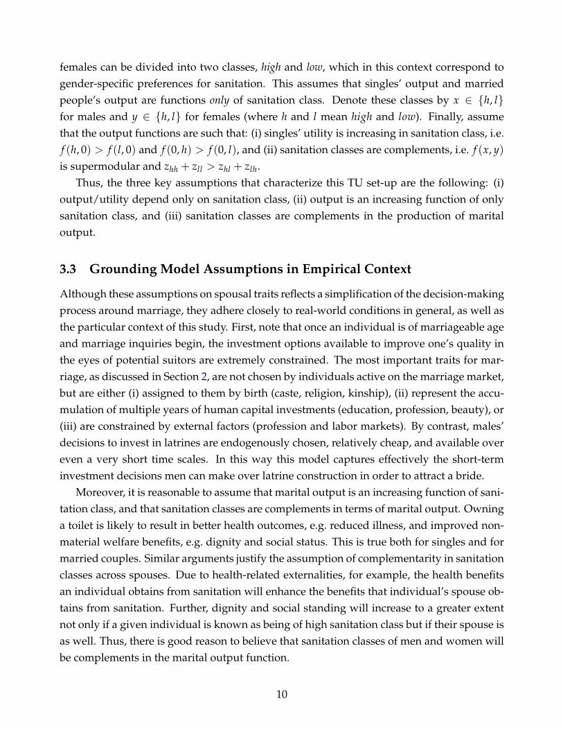
females can be divided into two classes, high and low, which in this context correspond togender-specific preferences for sanitation. This assumes that singles’ output and marriedpeople’s output are functions only of sanitation class. Denote these classes by x ∈ h, lfor males and y ∈ h, l for females (where h and l mean high and low). Finally, assumethat the output functions are such that: (i) singles’ utility is increasing in sanitation class, i.e.f (h, 0) > f (l, 0) and f (0, h) > f (0, l), and (ii) sanitation classes are complements, i.e. f (x, y)is supermodular and zhh + zll > zhl + zlh.

Thus, the three key assumptions that characterize this TU set-up are the following: (i)output/utility depend only on sanitation class, (ii) output is an increasing function of onlysanitation class, and (iii) sanitation classes are complements in the production of maritaloutput.

3.3 Grounding Model Assumptions in Empirical Context

Although these assumptions on spousal traits reflects a simplification of the decision-makingprocess around marriage, they adhere closely to real-world conditions in general, as well asthe particular context of this study. First, note that once an individual is of marriageable ageand marriage inquiries begin, the investment options available to improve one’s quality inthe eyes of potential suitors are extremely constrained. The most important traits for mar-riage, as discussed in Section 2, are not chosen by individuals active on the marriage market,but are either (i) assigned to them by birth (caste, religion, kinship), (ii) represent the accu-mulation of multiple years of human capital investments (education, profession, beauty), or(iii) are constrained by external factors (profession and labor markets). By contrast, males’decisions to invest in latrines are endogenously chosen, relatively cheap, and available overeven a very short time scales. In this way this model captures effectively the short-terminvestment decisions men can make over latrine construction in order to attract a bride.

Moreover, it is reasonable to assume that marital output is an increasing function of sani-tation class, and that sanitation classes are complements in terms of marital output. Owninga toilet is likely to result in better health outcomes, e.g. reduced illness, and improved non-material welfare benefits, e.g. dignity and social status. This is true both for singles and formarried couples. Similar arguments justify the assumption of complementarity in sanitationclasses across spouses. Due to health-related externalities, for example, the health benefitsan individual obtains from sanitation will enhance the benefits that individual’s spouse ob-tains from sanitation. Further, dignity and social standing will increase to a greater extentnot only if a given individual is known as being of high sanitation class but if their spouse isas well. Thus, there is good reason to believe that sanitation classes of men and women willbe complements in the marital output function.

10

3.4 Marriage Decisions

Conditional on sanitation class, individuals in the marriage market choose the class of thepotential spouse such that their share of the marital surplus is maximized. If the same con-ditions are met on the other side of the market, and if males’ and females’ respective sharesare greater than zero, then the marriage forms. Formally,

ux = maxUx + θx, 0 where Ux = maxy

[zxy −Vy

](2)

vy = maxVy + θy, 0 where Vy = maxx

[zxy −Ux

](3)

Individuals choose the partner of a sanitation class that maximizes their share of marital sur-plus, which is given by Ux (for men) and Vy (for women). Due to the simplification regard-ing sanitation classes, there are only four possible pairing: high/high, high/low, low/high,low/low. Further, the set-up implies that all individuals in the same group have an identicalsubstitute and therefore must receive the same share of marital surplus. In particular, ob-serve that if Uh is the share of marital surplus obtained by men in the high sanitation class,and Ul by those in the low sanitation class, then the difference (Uh −Ul) specifies the addi-tional surplus a married man receives from being in the high as compared to low sanitationclass.

3.5 Endogenous Investment

Let the marriage market economy be comprised of individuals who live for two periods.In period one, all men are in the low sanitation class, but can choose to invest in sanitationat cost c, which converts them into a high sanitation class individual in period two. Allinvestment decisions occur in the first period and all marriage decisions occur in the secondperiod. Assume lifetime utility is additive across periods. If men never marry and do notinvest, their lifetime two-period utility is given by 2 f (l, 0). If they do invest, then in the firstperiod they consume the output associated with a low sanitation person, f (l, 0), and in thesecond period consume f (h, 0) if they remain single.

The unmarried individual’s return to investing is the difference between individual outputas a high and low sanitation class person:

φx = f (h, 0)− f (l, 0) (4)

Putting this potential single individual’s return together with the marriage market return to

11

investment, the investment decision rule of males can be written as:

f (h, 0) + f (l, 0) + max [Uh + θx, 0]− c > 2 f (l, 0) + max [Ul + θx, 0] (5)

The left hand side of this inequality gives the total output consumed by men of high sanita-tion class after investing in period one; the right hand side gives total output conditional onnot investing.

As discussed above, decisions to marry are determined by the agents’ value of θ. Inparticular, if the individual emotional gain from marriage is sufficiently small (θx < −Uh),then even the largest possible share of the marital surplus will be insufficient to entice mento marry. Similarly, if the draw of θx is larger than −Ul, then the male will always marry,irrespective of investment decisions. Finally, there is an intermediate range of θx for whichmen marry on condition that they invested in the first period, and they remain single if theydo not build a latrine (−Uh < θx < −Ul).

3.6 Equilibrium

Equilibrium in this model is established by two criteria. First, a clear prerequisite for anystable matching profile is that equal numbers of men and women must marry. Formally,

r [1− F(−Vh)] = [1− F(−Ul)] +∫ −Ul

−Uh

G(φx + Uh + θx)h(θ)dθ (6)

where the left-hand side is simplified due to the assumption that female cost to being of highsanitation class is sufficiently low as to not impede females developing strong preferencesfor toilets.7

The first term on the right-hand side gives the proportion of men for whom the idiosyn-cratic gain from marriage, θx, is sufficiently large that they always marry. The second termreflects the proportion of men who marry because they made the premarital investment.The sum of these two terms must equal the sum of females, given on the left-hand side, whomarry. This quantity is mediated by r, which specifies the sex ratio of females to males. Ifr 6= 1, then incentives must adjust in order to equilibrate the numbers of available womenand willing men to marry.

The second criterion for equilibrium characterizes the relative proportions of men andwomen in high and low sanitation classes. Even if there are equal populations of men and

7More generally, if there is a cost to females of becoming high sanitation class, then they will face an in-vestment decision rule similar to 5. Later, when I discuss the “No Toilet, No Bride” campaign, this case can bemodeled as a shock that reduces dramatically the cost of females being high class. For example, if social normspreviously made it rare or difficult to negotiate over latrines, then “No Toilet, No Bride” made is less costly forwomen to express their preferences for sanitation.

12

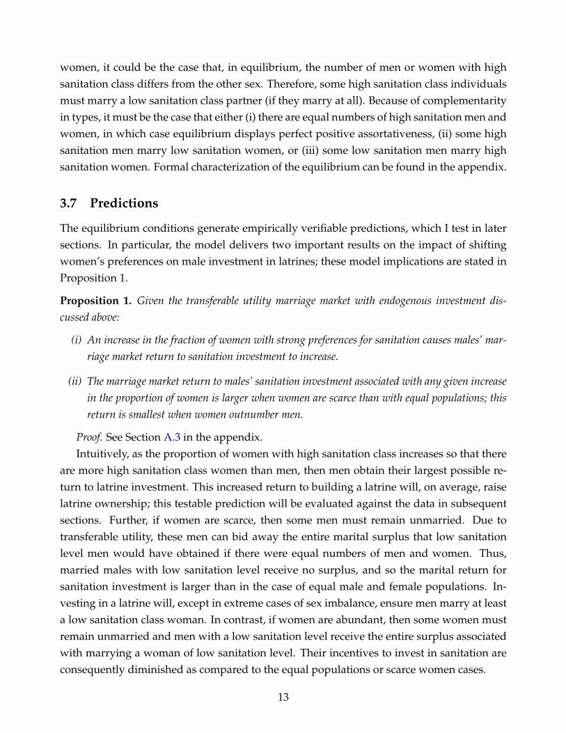
women, it could be the case that, in equilibrium, the number of men or women with highsanitation class differs from the other sex. Therefore, some high sanitation class individualsmust marry a low sanitation class partner (if they marry at all). Because of complementarityin types, it must be the case that either (i) there are equal numbers of high sanitation men andwomen, in which case equilibrium displays perfect positive assortativeness, (ii) some highsanitation men marry low sanitation women, or (iii) some low sanitation men marry highsanitation women. Formal characterization of the equilibrium can be found in the appendix.

3.7 Predictions

The equilibrium conditions generate empirically verifiable predictions, which I test in latersections. In particular, the model delivers two important results on the impact of shiftingwomen’s preferences on male investment in latrines; these model implications are stated inProposition 1.

Proposition 1. Given the transferable utility marriage market with endogenous investment dis-cussed above:

(i) An increase in the fraction of women with strong preferences for sanitation causes males’ mar-riage market return to sanitation investment to increase.

(ii) The marriage market return to males’ sanitation investment associated with any given increasein the proportion of women is larger when women are scarce than with equal populations; thisreturn is smallest when women outnumber men.

Proof. See Section A.3 in the appendix.Intuitively, as the proportion of women with high sanitation class increases so that there

are more high sanitation class women than men, then men obtain their largest possible re-turn to latrine investment. This increased return to building a latrine will, on average, raiselatrine ownership; this testable prediction will be evaluated against the data in subsequentsections. Further, if women are scarce, then some men must remain unmarried. Due totransferable utility, these men can bid away the entire marital surplus that low sanitationlevel men would have obtained if there were equal numbers of men and women. Thus,married males with low sanitation level receive no surplus, and so the marital return forsanitation investment is larger than in the case of equal male and female populations. In-vesting in a latrine will, except in extreme cases of sex imbalance, ensure men marry at leasta low sanitation class woman. In contrast, if women are abundant, then some women mustremain unmarried and men with a low sanitation level receive the entire surplus associatedwith marrying a woman of low sanitation level. Their incentives to invest in sanitation areconsequently diminished as compared to the equal populations or scarce women cases.

13

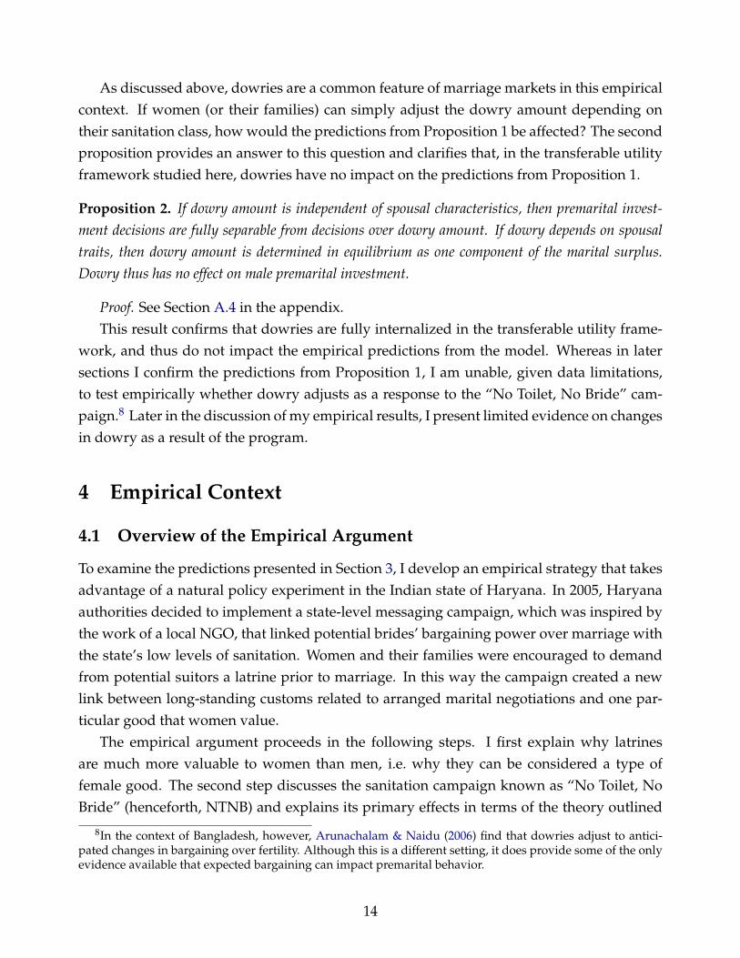
As discussed above, dowries are a common feature of marriage markets in this empiricalcontext. If women (or their families) can simply adjust the dowry amount depending ontheir sanitation class, how would the predictions from Proposition 1 be affected? The secondproposition provides an answer to this question and clarifies that, in the transferable utilityframework studied here, dowries have no impact on the predictions from Proposition 1.

Proposition 2. If dowry amount is independent of spousal characteristics, then premarital invest-ment decisions are fully separable from decisions over dowry amount. If dowry depends on spousaltraits, then dowry amount is determined in equilibrium as one component of the marital surplus.Dowry thus has no effect on male premarital investment.

Proof. See Section A.4 in the appendix.This result confirms that dowries are fully internalized in the transferable utility frame-

work, and thus do not impact the empirical predictions from the model. Whereas in latersections I confirm the predictions from Proposition 1, I am unable, given data limitations,to test empirically whether dowry adjusts as a response to the “No Toilet, No Bride” cam-paign.8 Later in the discussion of my empirical results, I present limited evidence on changesin dowry as a result of the program.

4 Empirical Context

4.1 Overview of the Empirical Argument

To examine the predictions presented in Section 3, I develop an empirical strategy that takesadvantage of a natural policy experiment in the Indian state of Haryana. In 2005, Haryanaauthorities decided to implement a state-level messaging campaign, which was inspired bythe work of a local NGO, that linked potential brides’ bargaining power over marriage withthe state’s low levels of sanitation. Women and their families were encouraged to demandfrom potential suitors a latrine prior to marriage. In this way the campaign created a newlink between long-standing customs related to arranged marital negotiations and one par-ticular good that women value.

The empirical argument proceeds in the following steps. I first explain why latrinesare much more valuable to women than men, i.e. why they can be considered a type offemale good. The second step discusses the sanitation campaign known as “No Toilet, NoBride” (henceforth, NTNB) and explains its primary effects in terms of the theory outlined

8In the context of Bangladesh, however, Arunachalam & Naidu (2006) find that dowries adjust to antici-pated changes in bargaining over fertility. Although this is a different setting, it does provide some of the onlyevidence available that expected bargaining can impact premarital behavior.

14

above. By focusing on women’s ability to demand latrines, the program provides a meansof studying their bargaining power on the marriage market. Subsequently, I show evidencethat the policy has indeed caused an increase in latrine ownership, that this effect is mediatedby the marriage market, and that sex ratios appear to be driving the program effect, furthersupporting the predictions of the marriage market model. Finally, I present complementaryevidence that the program appears not to have changed male preferences as opposed tofemale preferences, and evidence that the program caused an increase in latrine ownershiponly through the marriage market.

4.2 Sanitation, Gender, and the “No Toilet, No Bride” Program

4.2.1 Sanitation as a Female Good

In rural India, a large majority of people lack access to sanitation and must defecate in theopen. In a recent household survey conducted in Madhya Pradesh, for example, 80% of re-spondents reported that their primary places of defecation were fields, bushes, rivers/streams,and other public spaces rather than an improved latrine (Patil & Salvatore (2010)). Access tosanitation, and the lack thereof, affects all people but is of particular significance to women.It is, first of all, a matter of convenience to have a private toilet at home, to be used at one’swhim with little effort; this value exists for all members of the household. For women, how-ever, private latrines also provide significant benefits in terms of personal dignity and phys-ical security. The impact of sanitation on female dignity is reflected well in the comments ofa sixteen-year-old girl, who explained that “the toilet campaign is like a liberation. . . I wouldfeel so conscious and ashamed [setting off in the mornings toward the open fields]. Butjust before my brother got married, we got a toilet in the house."9 To mitigate embarrass-ment, Indian women often relieve themselves before sunrise or after dark, putting them atgreater risk of sexual assault and other attacks from either humans or, in many rural areas,dangerous wild animals.10

These strong preferences for privacy result in uncomfortable strategies to minimize ex-posure. It is common for women to refrain from drinking during the day in order to avoidneeding to use a toilet before sunset. Another respondent elaborated on this behavior: “Youcan spot men all over the hills and in the main town parking themselves on the side of theroads. But when we go down. . . we keep in mind that we shouldn’t consume too muchliquids, or else we might have to use the dirty loos. We have got used to holding it for-

9Source: Tehelka Magazine (Indian weekly), Vol. 7, Issue 29, July 24, 2010.10One respondent explained: “During the monsoons it is worse. In the dark when we visit the water logged

field overgrown with grass and floating with night soil, the danger of getting bitten by snakes and scorpionsis also high.” Source: Lesley D. Biswas, The Women’s International Perspective, October 1, 2010.

15

ever.” These coping mechanisms have psychological and physical consequences. “Womensuffer the most [from lack of sanitation] since there are prying eyes everywhere”, said AshokGera, a doctor who works in a one-room clinic in Haryana. “It’s humiliating, harrowing andextremely unhealthy. I see so many young women who have prolonged urinary tract infec-tions and kidney and liver problems because they don’t have a safe place to go”. Despitethese health effects, women rarely report health concerns as a motivation for toilets; theirrationales are most frequently framed in terms of privacy and dignity. This is evidence of astrong female preference for privacy in a social context characterized by routine male effortsto view any uncovered women. Finally, menstruation provides another significant reasonfor why women value private latrines: toilets provide females with the privacy, time, andcomfort necessary to attend to personal hygiene (World Bank (2005)).11 Thus, because of thehigh and gender-specific value that women ascribe, latrines can be understood as a type ofprivate female good.

4.2.2 The “No Toilet, No Bride” Program

In Haryana state, local authorities initiated a massive media campaign in 2005 organizedaround the message of respecting the right of women to use latrines in privacy and security.This campaign is part of India’s Total Sanitation Campaign (TSC), a national initiative of theGovernment of India whose primary objective is to ensure access to and use of sanitationfacilities in rural areas. Although a federal initiative, states shoulder a portion of the costsand have substantial flexibility in local design and implementation.

This information campaign encouraged the families of women to demand of boys’ fam-ilies that they construct a latrine prior to the woman marrying and relocating into the boys’family compound (Haryana, like the rest of northern India is predominantly patrilocal). Slo-gans such as “no loo, no I do" and “no toilet, no bride" were disseminated via radio, banners,and other advertising channels. In particular, village walls were painted with the message:“I won’t allow my daughter to marry into a home without toilets.” This initiative thus em-phasized a novel linkage between social norms around the marriage market and access tosanitation.

Popular media reports suggest widespread exposure to these ideas.12 In an interviewconducted by the Washington Post, a young male, age 22, who was hoping to marry soon,explained: “I will have to work hard to afford a toilet. We won’t get any bride if we don’t

11Many authors have argued this strong preference might drive absenteeism among girls in secondaryschool, despite the null findings of Oster & Thornton (2011), who do not report on the presence of sanitationfacilities in their sample schools in Nepal and/or whether latrines influence take-up of menstrual cups.

12See, e.g., The Times (UK): “Show us your loo before you woo, men are told” (March 26, 2009) and theWashington Post: “In India, more women demand toilets before marriage” (October 12, 2009).

16

have one now.” “I won’t be offended when the woman I like asks for a toilet,” he added. Aspart of the information and education campaign, blank building walls were converted intobillboards and painted with the slogan (in Hindi): “I won’t get my daughter married intoa household which does not have a toilet”. A recurring radio jingle sang a tune with thelyrics: “no loo, no I do.” The founder of Sulabh International, an NGO that designs low-costimproved latrines, states: “The ‘No Toilet, No Bride’ program is a bloodless coup. When Istarted, it was a cultural taboo to even talk about toilets. Now it’s changing. My motherused to wake up at 4am to find someplace [in the fields or rivers] to go quietly. My wifewakes up at 7am and can go safely in her home.” These vignettes help to characterize thesocial context in which the “No Toilet, No Bride” campaign operates.

In addition to anecdotal evidence, administrative data from the Haryana health depart-ment suggest a large increase in latrine ownership in recent years. According to state offi-cials, 1.42 million toilets were built between 2005 and 2009. Among this total, 950,000 latrineswere built by families above the poverty line and 470,000 by households below the povertyline. Further, household survey data provides additional support for the claim of increasedlatrine coverage. According to data from two rounds of the District-Level and HouseholdSurvey (these data will be described in greater detail below), the proportion of householdsthat owned improved latrines increased from 29% in 2004 to 41% in 2008.

Note that latrines are moderately costly capital investments. The average cost of an im-proved latrine (e.g. a pit latrine with protective slab or a flush toilet to septic tank) typi-cally ranges between 1000 and 2000 rupees (approximately $20–40 USD). For purposes ofcomparison, Haryana’s state-mandated minimum wage for “Scheduled Appointments” ofunskilled laborers was 135 rupees in 2004. According to the Indian NSS, Haryana has thesecond highest daily wage rate for agricultural labor (195 rupees). Therefore, the cost oftypical latrine will range from five to 14 days of paid labor for these two unskilled groups.However, the Government of India provides through the Total Sanitation Campaign subsi-dies that reimburse households for up to 80% of latrine costs if they possess a Below PovertyLine (BPL) card. Given this incentive scheme, households below the poverty line (BPL) areable to construct an improved latrine at an actual cost of approximately Rs. 200–300 (roughly$4.50–6.75 USD). This amount would be only two days labor for an unskilled worker atHaryana’s public position minimum wage or for an agricultural daily wage laborers withBPL card (NSS 2010).

5 Empirical Strategy

Haryana’s “No Toilet, No Bride” campaign can be understood as generating exogenous vari-ation in the proportion of women with strong preferences for sanitation. Thus, by studying

17

how latrine adoption responds to the program, it is possible to test empirically the predic-tions from the theoretical model.

I identify program effects by exploiting the following intuition. The program is targetedto girls and their families in the sense that the female side of the marriage market must ac-cept the campaign’s message and decide to take action. The female side of the market is thefirst step in the sequence of behavioral change related to latrine ownership. However, if theprogram is effective and women either express their preference or demand a latrine frompotential suitors, then the program will exert disproportionate pressure, which is plausiblyexogenous, specifically on those households that have boys of marriage age, i.e. householdswith boys active or nearly active on the marriage market. To study whether women are ableto demand and obtain latrines, therefore, I explore changes in latrine ownership among theseparticular households with marriageable boys, who comprise the actual treatment group inwhich the relevant outcome can be measured. After exposure to the program, householdswith boys of marriageable age can be expected to have a higher probability of latrine adop-tion as compared with households without marriageable boys.

Since the campaign began in 2005, households are unable to choose the number of mar-riageable boys as a response to program incentives.13 In this sense, program exposure inHaryana is plausibly exogenous to the presence of a marriageable boy. Still, householdswith marriageable boys might differ systematically from non-marriageable boy households,which raises concerns about endogeneity in any simple comparison of these two groupsover time.

To address these econometric concerns, I propose two complementary analyses. Estima-tion begins with a difference-in-difference (DD) specification, which controls explicitly forpotential differences in marriageable boy and non-marriageable boy households. I lay outthe identifying assumptions required for this analysis, discuss unresolved issues, and pro-pose an additional method based on significantly weaker assumptions. In particular, I use adifference-in-difference-in-difference (DDD) specification, which captures the change in thedifference between households with and without marriageable boys on ownership of a la-trine after the program was implemented, using northern Indian states other than Haryanaas a comparison group. As discussed in Section 2, these states are an appropriate choice forcomparison with Haryana because of their relative similarity on matters of son preferenceand sex ratios as compared to southern Indian or the easternmost Indian states. For thesereasons, the factors that mediate women’s bargaining power and marriage market processesare likely to be comparable across treatment and comparison households. Estimates of the

13Households could choose, of course, how and when to become active on the marriage market. The mannerin which I construct my marriageable boy variable, explained in greater detail in Section 5.2, addresses thisconcern explicitly.

18

NTNB program effect are shown to be consistent and similar in magnitude across the DDand DDD specifications, despite being based on different assumptions.

5.1 Data

This paper uses two rounds of household microdata from the District Level Household andFacility Survey (DLHS), a nationwide survey implemented by the Government of India totrack the national Reproductive and Child Health Program.14 The primary survey moduleinterviews a representative sample of ever-married women and gathers household infor-mation on maternal and child health outcomes, family planning and reproductive health,utilization of health care services, access to health facilities, and health knowledge. Addi-tional modules focus on household, village, and health facility characteristics, but I do notuse them in my analysis. The data form a repeated cross-section that is representative at thedistrict level for 601 districts in 34 Indian states and territories. I use the two latest surveyrounds, DLHS-2 (2004) and DLHS-3 (2008/9), which provide data immediately precedingthe project period as well as after three/four years of program exposure.15

I restrict the sample to focus on rural households from northern states, which are thosestates characterized by the strongest cultural preference for sons, as discussed in Section2.3.16 Using these restrictions, my 2004 data contains information on roughly 220,000 house-holds, including 12,500 in Haryana; the 2008 sample contains data on approximately 370,000households, including about 16,000 Haryana households.

5.2 Variable Construction

In my empirical analysis, I construct the following variables. Latrine is a binary indicator thatassumes the value of one if household i owns a private latrine that prevents contact betweenhumans and excreta, as per the standard definition of the Joint Monitoring Programme ofWHO and UNICEF; note that shared latrines and pit latrines without slabs do not meet

14DLHS is an initiative of India’s Ministry of Health and Family Welfare and is implemented by the Interna-tional Institute for Population Sciences in Mumbai.

15For the remainder of the paper, I will simply refer the DLHS-3 survey year as 2008.16The 16 states included in my sample are: Jammu and Kashmir, Himachal Pradesh, Punjab, Chandigarh,

Uttaranchal, Haryana, Delhi, Rajasthan, Uttar Pradesh, Bihar, West Bengal, Jharkhand, Orissa, Chhatisgarh,Madhya Pradesh, and Gujarat. My empirical results are robust to alternative sample selection that includesonly Haryana and adjacent states as well as a regional criterion that includes all states in the northwest quad-rant of the country. However, the policy that I examine in my empirical section is at the state-level. Therefore,due to matters of inference using clustered data, it is desirable to include the largest number of states thatcould serve as plausible controls. Given the close relationship between son preference and women’s outcomesin society, the most appropriate control group is comprised by those states with similar levels of stated sonpreference.

19

these criteria. I use this definition due to its operational relevance to governmental and non-governmental sanitation programs, including the Total Sanitation Campaign and “No Toilet,No Bride”. Moreover, the requirement that toilets be private to a household is closely relatedto women’s concerns around privacy and dignity, and is thus important in the context of the“No Toilet, No Bride” program.

The marriageable boy and girl variables, mboy and girl, are based on the gender-specificmean age of marriage +/− one standard deviation (and rounded to the nearest integer).This variable adopts a value of one for any household that has a boy/girl of marriageableage, irrespective of marital status. Given my empirical strategy, I am implicitly definingthe “No Toilet, No Bride” treatment group as those households with boys of marriageableage, the vast majority of which have been active on the marriage market during the pro-gram. I considered alternative definitions of the marriageable criterion, including one basedexclusively on single, unmarried children, one based on strictly married men, as well asone using different intervals around the gender-specific mean. Increasing the interval sizearound mean age at marriage is undesirable because it includes larger numbers of house-holds who might not be affected by treatment. Observe that the definition using singlesexcludes by construction any households with marriageable boy(s) who married after theprogram began, thereby eliminating from treatment sample exactly those households mostlikely to have responded to the program. At the same time, the use of strictly married youngmen as mboys would exclude households with marriageable boys who purchased a toilet inanticipation of marriage.17 My preferred definition, therefore, is the gender-specific meanage at marriage +/− one standard deviation because it best balances these concerns.

To account for unobserved household fertility preferences, I also construct another mboy-oriented variable that is the total number of mboys in the household divided by the totalnumber of living children. This variable provides a more robust test of the effect of mboyseven if there are unobserved changes in household fertility in Haryana, which are potentiallycorrelated with presence of an mboy. While I report the results from regressions that use thisfraction of mboys variable instead of simply the presence or absence of mboys, it will be seenthat this modified use of mboys does not alter in either a qualitative or quantitative mannerthe central findings.

My empirical definition of marriage market builds on the discussion in Section 2, where Ireviewed evidence that (i) nearly all women marry within their caste group, and (ii) nearlyall women move, upon marriage, to villages that are between 30 and 70 kilometers awayfrom their home villages. Taken together, these facts provide a natural means of defin-ing a given household’s marriage market. Unfortunately, the DLHS data does not contain

17Numerous popular media accounts contain interviews in which young men report they are building alatrine in preparation for the marriage market, even if a potential spouse is not yet identified.

20

geocoded data on households, nor does it identify previous residences, so I am unable todefine marriage markets in this explicitly spatial way. Instead, I assume marriage occurspredominantly within one’s administrative district. Districts in India are heterogeneous interms of area, but their size ranges are comparable to the ranges reported in the studies ofmarriage migration. For example, the largest district in Haryana is roughly 70 kilometersacross from the western to eastern administrative boundary, while the smallest district isroughly 17 kilometers in diameter. Thus, districts provide a reasonable approximation tothe distance across which marriages typically form.

The second descriptive fact from Section 2 used when defining marriage markets is casteendogamy, which refers to practice of marrying within one’s own caste group. For the pur-poses of this marriage institution, the relevant grouping is the jati, which is sometimes re-ferred to, imprecisely, as sub-caste. The jati is a community that plays the principal role inproviding one’s social identity, including providing potential marital partners, providingsome forms of insurance against consumption risk, and serving as a professional networkacross labor markets (Munshi & Rosenzweig (2006)). In the absence of this detailed, jati-specific data, I use the DLHS question on broad caste grouping. This variable represents anaggregation of finer social categories, but it still divides the sample population into four cat-egories (scheduled caste, scheduled tribe, other “backward”, and other).18 Finally, becausethe relatively large caste category of “other” might include more than one religion (and mar-riages almost never happen across religions), I also include religion in my marriage marketdefinition. Thus, a marriage market for the purposes of this paper will be those householdsin household i’s home district with marriageable boys/girls of the same caste grouping andreligion.

Finally, the variable for sex ratio is the ratio of women to men in a particular marriagemarket. I exclude households in marriage markets where either the number of marriage-able boys or girls is less than twenty individuals; this omits unusual and pathological (e.g.missing) values for the sex ratio. There exists substantial variation in the sex ratios acrossmarriage markets, despite the overall sex imbalance in the population.

Table I presents summary statistics on key variables for Haryana and comparison statesin each round of the survey. These two groups are comparable across a wide range of rel-evant observables, including household size, the fraction of households with and withoutmboys, male age at marriage, age of the household head, etc. Given the severity of sex imbal-ance in the Punjab region, which includes Haryana, there is a few percentage point differ-ence in the ratio of women to men, although the trend in similarly declining (i.e. becomingmore skewed against women) over time in both Haryana and control states. Note that thesex ratio is greater than one in Haryana in 2004 and in control states in both 2004 and 2008.

18These categories encompass 19.4%, 13.3%, 39.9%, and 27% of my sample, respectively.

21

There are two reasons why this is the case. First, the marriage market definition internalizesthe average age gap between men and women at the time of marriage. On average, menmarry girls that are 3.5 years younger than them. With population growth, each successive,younger cohort is larger than its predecessor. Thus, by defining marriageable boys and girlsin this way, the fact of sex imbalance due to son preference is countervailed by the impact ofpopulation growth. The second reason is that the variance of the distribution of female ageat marriage is lower than that for males. Hence, when I define the marriage market in re-spect to male and female mean ages at marriage +/− one standard deviation, the age rangefor males is two years larger for males than females. This additionally causes more males tobe included in a marriage market, thereby increasing the sex ratio.

Latrines are also substantially different across Haryana and comparison states. In datafrom both survey rounds, control states have mean latrine ownership that is nearly 10 per-centage points lower than in Haryana. One reason for this is that Haryana is wealthier thanmost of the states in the comparison group, and wealth is correlated with latrine ownership.Moreover, the overall trends in latrine ownership in Haryana and control states differ aswell. Observe that in the comparison states sample latrine ownership has actually declinedbetween 2004 and 2008. For this reason a difference-in-difference analysis that simply com-pares Haryana and controls over time would be inappropriate. But when I disaggregatelatrine ownership by mboy status, it can be seen the decline in the control group is actuallydriven by the non-mboy households; mboy households in this group have increased their la-trine ownership, on average, but to a lesser degree than in Haryana. In other words, thereis a two percentage point increase in latrines among mboy households in comparison states,but this increase is much greater in Haryana due to the incentives established by NTNB.Note that in the DDD framework, which is explained in more detail below, these differentialtrends across mboy/non-mboy households are explicitly controlled for, and so pose no threatto identification.19

5.3 Empirical Specification

To estimate the impact of Haryana’s “No Toilet, No Bride” campaign on improved latrineownership, I begin with a difference-in-difference specification that compares latrine own-ership between Haryana households with and without mboys before and after program ex-posure. This analysis highlights the core intuition driving the empirical strategy, namelythat NTNB targeted the behavior of mboy households in particular. I run a regression of the

19As an extra robustness check, I run the entire analysis on a sample of households that excludes any statesthat have declining latrine coverage. All estimates remain unchanged.

22

following form:

Latrineit = α + β1(mboyi × postt) + β2(mboyi) + β3(posti) + εit (7)

where mboy is an indicator variable that adopts the value of one if household i has a malehousehold member between the ages of 19–27 (males’ mean age at marriage +/− one stan-dard deviation) and εit is a household-specific iid error term that satisfies E(εit|X) = 0.

In addition to the primary definition of mboys, I use an alternative mboy variable that isthe fraction of mboys in the household divided by the total number of children. This alternatedefinition addresses potential concerns that unobserved household fertility could be corre-lated with women’s status. This DD specification controls for unobserved time-invarianttraits of mboy and non-mboy households, as well as secular trends in Haryana. The coef-ficient of interest β1 is therefore identified from changes in latrine ownership among mboyhouseholds over time. Consistent identification in this case depends on the common trendsassumption for mboy and non-mboy households, i.e. observed changes in latrine ownershipbetween these two groups of households would have been identical in the absence of theprogram.

One concern with this approach, which would invalidate the identifying assumption,is that an unobserved shock in Haryana is positively correlated with latrine ownership inmboy households or negatively correlated with latrine ownership in non-mboy households.For example, since mboy are on average slightly wealthier than non-mboy households, anyeconomic shock that differentially affects wealthier households could affect latrine owner-ship as well.

I address this concern about potential endogeneity by using a triple difference (DDD)regression specification, where the three differences are households with and without mar-riageable boys, in Haryana and comparison states, before and after (three to four years of)program exposure. I regress a binary variable for latrine in household i in state j at time t ona set of interactions and fixed effects:

Latrineijt = α + β1(mboyi × statej × postt) + β2(mboyi × postt) + β3(mboyi × statej)

+ β4(statej × postt) + β5(mboyi) + β6(haryanai) + β7(posti) + εijt (8)

where mboy is defined as both an indicator and a fraction, as explained above, and εijt is ahousehold-specific iid error term with E(εijt|X) assumed = 0 given the full set of fixed ef-fects and interactions X. The fixed effects control for unobserved time-invariant factors at thestate level and time-varying factors across both states. The double interaction terms allowthe relationship between marriageable boys and improved latrines to vary across states and

23

across time, in addition to capturing state-specific linear time trends. In this formulation,the primary coefficient of interest is β1 on the triple interaction, which captures the changein the effect of marriageable boys on latrine adoption in Haryana between 2004 and 2008relative to the change in effect of marriageable boys on latrine adoption in control statesbetween 2004 and 2008. This is the period during which the “No Toilet, No Bride” cam-paign likely generated additional social pressure on these households. Because I conditionon state-year fixed effects, mboy-state, and mboy-year interactions, β1 is identified throughHaryana-specific changes over time in differential rates of latrine ownership between house-holds with and without marriageable boys.

Consistent estimation of this saturated linear probability model requires that E(εijt|X, δjt) =

0, where X is a vector comprised of the mboy variable interacted with state and year dum-mies, and δjt reflects state-year fixed effects.20 This assumes that changes in this differentialacross states and time are orthogonal to unobserved determinants of latrine ownership. Inassessing the validity of this identification strategy, note that the most likely explanationsfor a positive effect of marriageable boys on latrine ownership can be ruled out by this em-pirical strategy. For example, if households with young male adults typically enjoy higherincome, which allows them to purchase latrines, we would expect to see a positive corre-lation between marriageable boy households and latrine ownership across both states, butwe would not expect a Haryana-specific change over time. Another rationale for an ob-served positive correlation between marriageable boy households and latrine ownership isthat transfers associated with marriage, such as dowry and gift-giving, could also facilitatelatrine ownership. A similar counterargument, however, can also rule out this hypothesis:we would expect this story to affect households with marriageable boys equally in Haryanaand control states.

For the identifying assumption to be invalid, an unobserved factor must cause the trendin the difference in latrine ownership between households with and without marriageableboys to diverge across Haryana and control states. In such a case, this factor would causethe common trends assumption to be violated, i.e. the trend in the differential betweenmboy/non-mboy households would inaccurately reflect the counterfactual scenario in Haryanain the absence of the program. This identifying assumption would be violated if there areunobserved Haryana-specific shocks that covary with latrine adoption and the presence of amarriage age boy. This assumption is impossible to accept with certainty, but it is difficultto generate hypotheses on the types of shocks on Haryana’s marriageable boy householdsthat would undermine identification. With that said, Section 6.3 explores this robustness

20The linear probability model is particularly appropriate in this context because the fully saturated specifi-cation implies the conditional expectation function of latrine ownership is linear. Still, I run similar regressionsusing probit and logit specifications, which yields nearly identical results.

24

of this assumption to concerns about Haryana and mboy-specific shocks related to wealthand household size. Finally, I present additional findings that lend further support to themarriage market channel interpretation of observed changes in latrine ownership amongmarriageable boy households, thereby providing further, indirect support for this identifi-cation strategy.

6 Empirical Results

The empirical analysis presented in this section tests the two implications derived from themodel of marriage matching with endogenous investment.

6.1 Marriageable Boys and Household Latrine Adoption

I focus first on the main program effect of “No Toilet, No Bride” on latrine ownership; thisanalysis corresponds to the first theoretical prediction from Proposition 1. Recall that be-cause the program generates plausibly exogenous variation that increases the proportion ofwomen with a strong preference in toilets, the model predicts that latrine adoption shouldrise.

The first test of this prediction uses the DD specification given by (7); estimates are pre-sented in Table III. The DD estimates suggest that NTNB has increased mboy’s investmentin latrines by between 0.057 and 0.061 percentage points over a baseline mean of 0.27, i.e.NTNB increased latrine ownership by approximately 22%. When using the mboy fractionvariable that controls for household fertility, which is reported in columns (3) and (4), re-sults are similar, although the point estimates when including controls is somewhat smaller.

As suggested earlier, however, any changes in mboy households, e.g. wealth shocks,would violate the identifying assumption in this DD framework and yield inconsistent esti-mates. Therefore, I turn to the DDD analysis, which relies on significantly weaker assump-tions than the DD framework. Table II provides an intuitive preview of my main findingsregarding the treatment effect of “No Toilet, No Bride” on households with marriageableboys. This table contains mean latrine ownership among the eight possible groupings im-plied by the DDD strategy. For exposition, I compare Haryana only with Punjab, which isthe state most similar in terms of culture and economy. Punjab is, in fact, the ideal controlfor Haryana due to their long and common history as part of the greater Punjab region. Thisevidence must be considered suggestive; statistical inference is complicated by the fact thatpolicy variation occurs at the state-year level.

For this reason, the preferred DDD analysis includes a much larger sample of states,which have similar son preferences to Haryana. Table IV presents DDD estimates of the

25

NTNB campaign on latrine adoption. The primary coefficient of interest is the first tripleinteraction, which is positive and statistically significant (β = 0.043). The program increaseslatrine ownership by 4.3 percentage points above a baseline mean of 0.28 for Haryana’s mboyhouseholds, i.e. a 15% increase among those households likely to be affected by femalesdemanding/desiring improved sanitation.

These results support the argument that the more simple difference-in-difference speci-fications (instead of the full DDD implemented here) would provide inconsistent estimatesof the program effect. For example, Haryana increased state-level latrine ownership at afaster rate than control states, violating the common trends assumption in a DD framework.Moreover, mboy households in Haryana have, on average, a 3% lower probability of latrineownership, which again suggests a DD analysis at the Haryana/control level is problematic.These changes are explicitly controlled for as part of my identification strategy, as discussedabove.

The key result from this specification is the marked shift in the effect of marriageableboys on improved latrines, specific to Haryana after the NTNB campaign. Specifically, therewas a 4.3 percentage point change in the differential over time between Haryana and controlhouseholds with and without marriageable boys. Because the program targeted specificallythose households whose boys are on the marriage market, and having a marriageable boyis plausibly exogenous to household decisions regarding improved latrines, conditional onthe full set of interactions and fixed effects, these results provide evidence that either (i)a positive fraction of marriageable women in Haryana have shifted their preferences andpressured men into sanitation investments, or (ii) men have anticipated this pressure andresponded by increasing their premarital investment in latrines. There is an additional pos-sibility, outside of the bargaining interpretation, which suggests that new couples invest inlatrines as a form of health-seeking behavior and health investment in children.21 While theDDD specification cannot rule out this possibility, the following sections present evidenceon each of these channels and confirm that the marriage market hypothesis is driving theseresults.

6.2 Marriage Markets, Female Preferences and Latrine Adoption

The second testable prediction from the model states that the impact of rising proportionsof women with a preference for toilets on premarital investment will be mediated by the sexratio. To study this cross-partial effect of how sex imbalance in the marriage market mediates

21This hypothesis of unitary household preferences for investment in children is ruled out by the analysis ofsex ratios below. If women favor child investments more than men, however, then Haryana women demand-ing toilets, and therefore program effects, could be explained more by child health than private female benefits.This interpretation is fully consistent with the bargaining interpretation of the empirical results.

26

male investment responses to changing female preferences, I use regression specification(8) in two subsamples, where one is comprised of households in marriage markets withan oversupply of women and one with an undersupply of women. This formulation isdesirable for expositional purposes, but it is equivalent to interacting the sex ratio indicator(for r greater or less than unity) with the set of interactions and fixed effects from (8). Asbefore, I first present estimates from the DD (using mboy/non-mboy and pre/post treatment)and then turn to the preferred DDD analysis.

Tables V and VI report estimates from these analyses. When women are abundant, theestimated average treatment effect of NTNB is statistically indistinguishable from zero. Bycontrast, when woman are scarce and the marriage market is highly competitive for men, thetreatment effect is nearly double the estimate from the entire sample; this point estimate islarge and highly statistically significant (at the 99 percent level). The difference in magnitudeis nearly double the estimated effect from Table IV, which is consistent with the relative sizesof the subsamples, these results, and the earlier estimate that ignored the sex ratio.

These results provide strong evidence that skewed sex ratios mediate the impact ofwomen’s ability to demand latrines on the marriage market. When women are scarce, theyare able to negotiate successfully for latrines, but when they are abundant, men have less in-centive to invest and women are unable to obtain latrines to the same degree. In this sense,the phenomenon of missing women in a marriage market appears to have increased femalebargaining power, conditional on survival to marriage age. Finally, these results lend ad-ditional support to the marriage market hypothesis because evidence of marriage market-driven latrine adoption bolsters the case that NTNB exerted disproportionate pressure onmarriageable boys.

One issue that arises when interpreting these results is the role of migration. Perhapsmales elect to move out of tight marriage markets with dim prospects, or alternatively, theyimport brides from other marriage markets. Similarly, males could seek brides from youngercohorts, which will be larger than older cohorts, on average, because of population growth.There are in fact a wide variety of possible means by which men could relax the constraintsimposed on them in a particular marriage market. Unfortunately, the DLHS data do notcontain information that allows me to identify such migration. To the extent men are ableto alleviate the pressure they experience on the marriage market, however, my estimates ofthe program effect will underestimate the program effect in the absence of migration acrossmarriage markets.

27

6.3 Investigating Competing Hypotheses

The previous sections provided a series of results that together provide compelling evidencethat male premarital investments respond to both changing distributions of preferences inthe female populations and constraints generated by local sex imbalances. In this section Iconsider three competing interpretations of my main results. The first two hypotheses ex-plore distinct mechanisms by which the observed changes in latrine ownership might arise,which are outside the marriage market considerations reflected in the theoretical framework.The third hypothesis is a placebo test that examines whether any unobserved factors relatedto household size and/or fertility are driving my results. Given the tests conducted here, Ican strongly reject each of these competing hypotheses regarding the NTNB effect.

6.3.1 Does the Program Change Male Preferences?

Depending on how NTNB messages are received by men, the main empirical result fromSection 6.1 could arise not because women are exerting pressure via the marriage market onmale investments, but because men’s preferences have changed in response to the program.Consider a scenario whereby NTNB changed young adult male preferences for sanitationamong both households with boys active on the marriage market as well as those with rela-tively recent experience on the marriage market. Perhaps the program raised the salience ofsanitation in Haryana, changed men’s preferences, and thereby caused an increase in latrineadoption. In this way households with young men, which are relatively wealthy, becameconvinced about the value of sanitation and made the sanitation investment.22 Then even inmy triple difference empirical framework it might be possible to observe a program effect,yet this hypothesized shift would operate entirely outside of the marriage market.

I test this hypothesis directly by studying whether NTNB has caused any change in la-trine adoption among households with men slightly older than marriageable age. Recallthat my definition of marriageable boy is +/− one standard deviation from males’ meanage at marriage; this yields an age range of 19 to 27. Here I create a new indicator that takesthe value of one if a household has anyone in the age range 27 to 34 years. This age group isyoung and close enough in age to serve as a reasonable comparison group to very late teensand twenty-something year olds, but due to their age are almost certainly married alreadyand therefore immune from marriage market pressures generated by the program. I run aregression using the same DDD specification as above, but substitute the oldboy variable forthe mboy variable in all interactions and fixed effects.

As can be seen in Table VIII, the main coefficient of interest is statistically zero. Thesehouseholds, like mboy households, are more wealthy on average than households without

22Wealth and mboys are correlated in my sample (ρ = 0.11).

28

these oldboys. Given the focus on a cohort of men who are otherwise likely to be very sim-ilar to younger men active on the marriage market (if anything, they should have moreincome/wealth, on average, which they could use to purchase a latrine), the null resultsuggests that male preferences have not changed as a result of the NTNB program. Thisprovides additional evidence that the mechanism through which the program operates isthe marriage market hypothesis.

6.3.2 Do Changing Female Preferences Drive Latrine Adoption Outside of Marriage?

A second possibility regarding the behavioral mechanism driving latrine adoption is thatfemale preferences are indeed changing as a result of NTNB, but that these preferences af-fect latrine ownership outside of marriage market channels. For example, girls might learnfrom the NTNB emphasis that latrines are valuable and subsequently push their parents orhusbands into buying them. Under this hypothesis, women still push for latrines as a resultof the program but they obtain the goods for reasons that have nothing to do with marriageper se.

To study this issue, I use a DDD regression that focuses on mgirls in place of mboys. Yetmany households with both mboys and mgirls will be married, so running this analysis onthe entire sample will include all those households in which men built a latrine in order tomarry. In this case it would be impossible to distinguish between the effects of premaritalbargaining and investment on the one hand and changes in female preferences outside ofthe marriage market. Instead, I focus on a subsample that excludes households with bothmarriageable boys and marriageable girls. Some of these households will have both mboysand mgirls because they are siblings; it is unfortunate that they are excluded but the datadoes not allow me to differentiate perfectly between sibling pairs and married pairs. Thebenefit of analyzing this subsample, however, is that it excludes with near certainty thosecouples who married since NTNB began, thereby focusing the analysis on single mgirls.

Table IX reports the results from this analysis. In this case, the coefficient of interest isagain statistically indistinguishable from zero. This suggests that among girls who are activeon the marriage market, and who are thus a primary target of the NTNB message, there isno program-induced ability to obtain latrines. These results provides an instructive coun-terpoint to the results from Table IV. In that case, women are able to obtain latrines throughmarriage, in accordance with their preferences. But when these marriages are excludedfrom the sample, we observe no program effect at all. Therefore, the evidence indicates thatNTNB causes women’s preferences to shift, but that this causes a shift in male premaritalinvestments only through marriage market pressures.

29

6.3.3 Omitted Variables Correlated With Household Size

Earlier I noted that the key identifying assumption underlying my econometric specificationcould be violated if there exists an unobserved, differential trend that affected only mar-riageable boy households in Haryana. For example, if Haryana instituted an anti-povertyprogram between 2005 and 2008, which raised incomes of marriageable boy households,then increased toilet coverage could be explained by an income rather than marriage marketeffect associated with the program. If this were the case, E(εijt|X, δjt) 6= 0 and estimates ofβ1 from eq. (8) would be biased.

Household structure might play a particularly important role in this context because ofthe strong son preference in the greater Punjab region. One form this son preference cantake is fertility behavior that follows a stopping rule, i.e. when families have children untilthey have a boy, who will continue to live in the family compound and care for the parentsin old age (girls will typically marry and move away from the village). If households prac-tice a stopping rule, then households with any girl children will be, on average, larger andslightly older than households without girls. This reasoning suggests that the demographicand age structure of the household might vary systematically with the gender composi-tion of the children. Additionally, because household size is correlated with poverty, anyHaryana-specific anti-poverty program after 2005, such as (hypothetically) workfare or low-income educational stipends, could also cause a spurious correlation between marriageableboy households in Haryana in 2008 and latrine ownership.

My alternative definition of mboy as the fraction of mboys among total children in thehousehold provides on strong test of the influence of unobserved fertility on latrine adop-tion. In addition, I test the validity of this hypothesis by modifying eq. (8) by adding the fullsuite of interactions and fixed effects for two different categories of household size. Specif-ically, I create a dummy variable for small households that indicates whether the householdis smaller than the mean household size in the sample; large households are those larger thanmean household size. My main empirical specification, modified in this manner, tests simul-taneously for both potentially confounding stories just outlined.

As can be seen in Table VII, the primary coefficients of interest are, as before, only thetriple interaction terms that reflect the DDD for marriageable boys, small households, andlarge households in Haryana in the post-treatment period. I find small and statistically in-significant effects for both small and large households, and the estimate of the NTNB treat-ment effect, captured in the mboy triple interaction, remains positive and significant at thefive percent level. These robustness results provide evidence rebutting the notion that fac-tors related to the age or demographic structure of households are confounding my esti-mates of the program effect.

30

7 Bargaining Power and the Intrahousehold Allocation

The theoretical literature on collective household and marriage models suggests that mar-riage market conditions, such as sex imbalance or divorce laws, should affect the intrahouse-hold allocation by shifting the resource sharing rule toward the scarcer sex. Thus, theoret-ical investigations predict that female scarcity should result in greater bargaining poweramong the remaining women. In this sense, sex ratios are a prototypical distribution fac-tor (Browning & Chiappori (1998)), i.e. a condition that alters the household sharing rulewithout changing the joint budget set or individual preferences.

Until now, this paper has focused on how marriage market conditions affect male invest-ments in a good women value highly. I presented evidence that the program appears tooperate by changing female preferences in conjunction with marriage market pressures re-lated to sex imbalance. But these results are consistent with two possible mechanisms, bothof which operate through the marriage market. Does the program indeed cause a shift infemale preferences for sanitation, making them stronger than before? Or does the program’semphasis on female bargaining power on the marriage market actually increase that powerdirectly? In other words, the program might shift the distribution of female types and, by sodoing, drive male premarital investment, or it might act as a sort of distribution factor thatitself shifts the intrahousehold sharing rule.

It is less plausible that an information campaign can act in a distribution factor than serveto shift preferences. Yet these two mechanisms carry strong implications for how householdbehavior responds to the program. In particular, the former interpretation suggests the pro-gram taps into the relative bargaining power held by women when they are scarce, changeswomen’s preferences over the bundle of assets and qualities of marriage that they bargainover, and so causes women to negotiate more readily over latrines as compared to other de-sired goods. If this interpretation is correct, then we would expect to see that the observedtreatment effect on latrines results in a form of compensating differential with respect toother goods, i.e. women must trade off some good(s) in order to obtain a toilet at the time ofmarriage. And the second interpretation is that by highlighting women’s right to demandcertain goods, particularly if not only in the context of female scarcity, the program providesan exogenous, positive shock directly to women’s bargaining power rather than to femalepreferences. In this case, we would expect to see an unconditional increase in latrines as anet gain for women, i.e. without any tradeoffs.

I examine the first interpretation that the program changed female preferences, redis-tributing relatively more weight to latrines and less weight to other items in the bundle ofgoods that women value. Greater latrine ownership in response to the program should oc-cur when women have sufficient bargaining power to obtain goods they particularly desire.

31

Moreover, if the program causes an alteration of the woman’s weighting scheme over herpreferred goods, then the program effect should also cause a decline in ownership of someother favored good. We should therefore find evidence that women must trade off somegoods they prefer in order to secure latrines during the marriage bargaining process.

Note that if one is prepared to assume that women would never agree to a trade (of alatrine for some other good or bundle thereof) that lowered her utility, then one can im-mediately conclude that the increase in latrine adoption reflects a shift in the intrahouseholdallocation toward women that has unambiguously improved female welfare. Absent this as-sumption, it is possible to explore a range of household goods and characteristics for whichwe have reason to believe women have a strong preference. Given the cultural context ofHaryana, such marriage qualities might include the educational levels of one’s spouse (con-ditional on own education), the age gap between husband and wife (younger brides relativeto men are associated with lower status of women in the household; see, e.g., Desai & An-drist (2010)), influence over fertility, and/or increased access to household assets such asimproved cooking fuels, sewing machines, washing machines, etc.

I test for program effects for each of these outcomes using the DDD approach, when thereis data on the particular asset or outcome for both survey rounds, or using DD (with the dif-ferences being mboy/non-mboy households in Haryana and control states), when there existsdata only from the 2008 round. Table X summarizes the findings from these regressions. Theunifying result is that along a range of numerous possible goods and desirable traits, thereis no evidence that women have been forced to tradeoff other desirable goods in order tosecure a latrine.

In contrast, these results provide suggestive evidence that the relative position of womenhas improved, in addition to latrines, along two key dimensions: the education level of thehusband, conditional on women’s education, and the age at marriage/living with husband.With respect to the education difference between husband and wife, a simple analysis ofthe DDD estimates does not yield statistically significant differences. Disaggregating thedata into those households with and without latrines, however, indicates an increase in 0.1years in the differential between male and female schooling specifically among mboy house-holds in Haryana post-treatment; in these same households without latrines, there appearsto have been a 0.03 year decline in the gap but this is not statistically significant; the statis-tically significant difference between these estimates is 0.13 years. The evidence thereforesuggests a slight improvement in the average quality of males for a given female only inthose treatment households with latrines.

With respect to female age at marriage, a trait which is positively associated with femalestatus, a pattern similar to the education gap emerges. That is, the DD estimate of changesin age at marriage that arise among mboy households in Haryana is not statistically signifi-

32

cant, but it appears to mask heterogeneity across households with and without latrines. Inparticular, there appears to be an increase of 0.16 years in the mean age at marriage, whichis specific to households that have latrines who are therefore likely to have responded to theprogram. In mboy households without latrines, however, no such evidence emerges. Hence,women in mboy households in Haryana after treatment appear to get married slightly later(0.24 years) in those households that have latrines as compared to Haryana mboy householdswithout latrines. A similar result was found with respect to the age at which the female firstcohabits with the husband.

One interesting result to emerge is that there has been an increase in motorbike own-ership. Motorbikes are a good that males value and that form a common part of dowryamong wealthier families. The observed increase among mboy households in Haryana afterprogram exposure occurs for both mboy households that have latrines as well as those thatdo not, but those with latrines have a (statistically significant) two percentage point higherprobability of motorbike ownership than households without latrines after the program.This quantity reflects a 7% increase in motorbike ownership associated with being a treat-ment household and having a latrine. This result provides suggestive evidence that marriagenegotiations over toilets have been associated with men being compensated in other waysfor the expense.

Taken together, these suggestive results indicate that NTNB and bargaining over latrinesmight have caused a number of shifts in dowry outcomes, but there is no evidence that fe-males were forced to substitute items they care about in favor of toilets. On the contrary, itappears that women have improved their relative position in the household on account ofmarrying older and marrying better educated men, while Haryana’s mboys have increasedtheir ownership of motorbikes, especially if they built a latrine. Dowries, which are unob-served, could play a fundamental role in driving these findings. It seems likely that severalitems commonly involved in dowry and marriage negotiations might have shifted in re-sponse to the program, but without additional data and assumptions on the household’sbehavior it is impossible to empirically determine a shift in the intrahousehold allocation.

8 Conclusion

This paper focuses on an innovative natural policy experiment known as “No Toilet, NoBride”, which highlighted the link between latrines, for which women have a strong pref-erence due to concerns about privacy and security, and marriage markets in Haryana statein the historical Punjab region. Because the program encouraged girls’ families to demandfrom boys’ families a latrine prior to marriage, it generated disproportionate pressure to con-struct a latrine specifically among those households whose boys were of marriageable age

33

and seeking a bride. I demonstrate that marriageable boy households were indeed affecteddisproportionately by the program, and I estimate the “No Toilet, No Bride” treatment effectto have increased latrine ownership by 15% over the baseline mean of Haryana householdswith marriageable boys in 2004. In addition, estimates of latrine adoption in Haryana post-treatment are four times larger in marriage markets characterized by a scarcity of women ascompared to marriage markets with more women than men.

These results are shown to be invulnerable to competing hypotheses that challenge thismarriageable boy effect of the program. In particular, I have shown (i) there is no evidencethat unobserved factors correlated with household size are driving my estimates and (ii) theprogram does not appear to have changed male preferences for latrines. The “No Toilet, NoBride” program thus appears to have caused a significant increase in latrine ownership inHaryana specifically through the channel of female preferences in the context of bargainingpower. Moreover, I provide substantial evidence that women are not trading toilets for othergoods in the context of marriage bargaining toilets. Indeed, the program is associated withan increase along two fundamental dimension for women’s status: the mean age at marriageand educational quality of the husband. These findings are consistent with a theoreticalframework in which sex imbalance alters marriage market conditions and causes males toincrease their premarital investments in their own quality.

The underlying mechanism that drives latrine adoption among households with mar-riageable boys is thus competition on the marriage market and a household’s desire to marrysuccessfully its boys. In exploring the impact of skewed sex ratios on women’s bargainingpower, as reflected in female demand for latrines under “No Toilet, No Bride”, this pa-per provides evidence that, despite widespread and persistent discrimination, the femalebargaining position has improved through heightened competition on the male side of themarket.

In addition to the literature on female bargaining power and marriage, this paper alsomakes an important contribution to the limited evidence that exists on the effectiveness ofsanitation campaigns at large scale. In India, nearly 70% of the rural population lacks accessto sanitation, and this situation is associated with severe morbidity and mortality. An esti-mated 1.2 million children under five die each year in the country; most of these deaths areattributed to diarrheal disease and acute respiratory infections, which are both exacerbatedby inadequate sanitary behavior and sanitation infrastructure (Black et al. (2003)). In thiscritical policy context, a low-intensity information campaign, “No Toilet, No Bride”, cleverlyexploited deeply rooted social norms and marriage market conditions in order to increasesanitation. As a result, there are approximately 500,000 more toilets among Haryana’s fourmillion households in 2008 than in 2004.23 By studying this large shift, this paper is infor-

23This number reflects the increase in toilets in Haryana that can be attributed to the “No Toilet, No Bride”

34

mative not only about female bargaining power, but also regarding the design of sanitationpolicy and behavior change programs more generally.

campaign based on estimates in this paper.

35

A Theoretical Appendix

A.1 Additional Features of Transferable Utility

The assumption underlying the transferable utility framework is that this marital surplusis divided and shared between spouses. In particular, the surplus is divided according to asharing rule that is determined not by the individual characteristics of partners in a match,but by the requirements imposed by stable matching. A matching assignment profile is con-sidered stable if no two married or unmarried people prefer to be together and no marriedindividual prefers to be single (Gale & Shapley (1962)). This profile will display either pos-itive or negative assortativeness depending on the super- or sub-modularity of the maritaloutput function f (x, y), i.e. whether traits x and y are complements or substitutes.24 Thenthe key feature of transferable utility is that a man (woman) with a given level of quality can“bid away” higher quality men (women) by offering the potential spouse on the other sideof the market a greater share of the marital surplus. The well-known consequence is thatthe equilibrium, i.e. the stable assignment profile, must maximize aggregate marital surplusacross all men and women (Shapley & Shubik (1972) and Becker (1973)). Moreover, thesharing rule that specifies the division of the marital surplus is determined in equilibriumthrough the requirements of stable matching. In this way, changes in the relative propor-tions of men and women, or in the distribution of quality in the male or female populations,alter the sharing rule over marital surplus.

A.2 Further Characterization of Equilibrium

To characterize equilibrium formally, let α denote the fraction of women of high sanitationclass; (1− α) is therefore the fraction of women with low sanitation preferences. Similarly,define β as the fraction of men who have invested in a latrine and so are of high sanitationclass; (1− β) gives the complementary set of men who did not invest. The second criterionfor equilibrium can then be expressed for each possible scenario outlined above, i.e. α = β,α > β, and α < β.

The first case, when equal numbers of high sanitation class people get married, is thefollowing:

α = [1− F(−Ul)] G(φx + Uh −Ul)︸ ︷︷ ︸Always marry and invest

+∫ −Ul

−Uh

G(φx + Uh + θ)h(θ)dθ︸ ︷︷ ︸Married b/c invested

= β (9)

24This paper assumes throughout that positive assortativeness holds.

36

The second and third cases involve the possibility that, in equilibrium, more men orwomen belong to the high sanitation class and thus some individual(s) in the high groupingmarry individual(s) from the low grouping. Formally, these cases are:

α > [1− F(−Ul)] G(φx + Uh −Ul) +∫ −Ul

−Uh

G(φx + Uh + θ)h(θ)dθ (10)

α < [1− F(−Ul)] G(φx + Uh −Ul) +∫ −Ul

−Uh

G(φx + Uh + θ)h(θ)dθ (11)

Eq. (10) states there are more women with high preferences for sanitation than men who in-vested in latrines. Eq. (11) considers the opposite case when more men invested than thereare women with high preferences for sanitation. Note that the assumption of complemen-tarity of types implies that only one of these inequalities can hold at once. These expressionscombined with equation (9) specify the equilibrium. See Chiappori et al. (2009) for a proofof existence and uniqueness of this marriage market equilibrium.

A.3 Division of the Marital Surplus

The equilibrium conditions have strong implications for the sharing rule that divides maritalsurplus. Consider each of the three cases in turn. In the first case, when α = β, there isperfect positive assortativeness. Thus, the surplus from marriage of same types, zhh or zll,must equal the sum of shares from two same-class individuals marrying, that is:

zhh = Uh + Vh (12)

zll = Ul + Vl (13)

Male and female shares need not be equal if the outside options to marriage differ acrossspouses.

When α 6= β, then surplus shares must satisfy:

Uh + Vl ≥ zhl (14)

Ul + Vh ≥ zlh (15)

In particular, when α < β, there are more men who invested than there are women withstrong preferences for sanitation, and eq. (14) will hold with equality while eq. (15) willhold as a strict inequality. An immediate consequence of these equilibrium shares is thathigh sanitation men must relinquish some of the marital return from their investment. Inparticular, they must receive their lower-bound marital return to investment; otherwise, anequivalent man could bid away any surplus until the minimum bound is restored. Plugging

37

eq. (14) into (12) and using (13) yields:

Vh −Vl = zhh − zhl (16)

Uh −Ul = zhl − zll (17)

Eq. (17) specifies the marriage market return to investment by males, and men get only theirmarginal contribution to a marriage with a low sanitation class woman, i.e. the lower boundon their investment return. By contrast, women with high sanitation preferences get theirentire contribution to the marital surplus of a marriage with a man with a high sanitationclass. By contrast, when α > β, men receive the entire marginal contribution to maritalsurplus from their investment (= zhh − zlh), and women receive the remainder (= zlh − zll).

These bounds on the marriage market returns yield testable results. I gather the keypredictions from this discussion into Proposition 1, which is presented in Section 3.7 above.

Proof. I consider each of the two main testable predictions in turn.Observe that eq. (9) implicitly defines males’ marriage market return to investment (Uh−

Ul) as a function of α. As α increases, it immediately follows that either Uh must increaseand/or Ul decrease in order for there to be sufficient men willing to marry (conditional oninvesting). Thus, an increase in α drives male premarital investment by increasing males’marriage market return.

For the second implication, consider eq. (6) when θy > −Vh and all women want to marrysomeone.25 Assume r < 1 and women are scarce. This implies that some men must remainunmarried. As r decreases, Vh and Ul must decline and/or Uh must increase, which impliesthat the marriage market return to male premarital investment increases (and women’s mar-riage market return to being of high sanitation class must decline) to maintain equality inthe numbers of men and women who want to marry.

In the case of equal populations, i.e. r = 1, an increase in the fraction of females withstrong preferences for sanitation causes men to receive their upper bound return on sanita-tion investment. Now consider a situation of female scarcity. Some proportion (1− r) menwill fail to marry, even if they want to, because of an insufficient number of brides. Thesepotentially unmarried men, who will all be of a low sanitation class, will bid away the entiresurplus obtained by the married low sanitation class men, i.e. Ul decreases. The immediateconsequence is that Uh−Ul is larger than in the case of equal populations. Conversely, whenr > 1 and women outsupply men, then low sanitation level men receive the entire surplusin a marriage with a low sanitation type female, i.e. Ul increases as compared to the case of

25This situation in which the idiosyncratic gain from marriage for females is sufficiently large to cause allwomen to prefer marriage is easily justified given the particularly low status ascribed to older single womenin Haryana.

38

equal populations. Therefore, Uh −Ul must be smaller when r > 1 than when r = 1, whichis in turn smaller than when r < 1. In this way, the second part of Proposition 1 followsdirectly from transferable utility and the requirements of pairwise stable matching.

A.4 Dowries

In a transferable utility (TU) framework, dowries form a part of the transfers that dividethe surplus. Thus, a natural way to incorporate dowry is to assume that marital output iscomprised of two portions: non-dowry and dowry output, i.e. the marital output = f (x, y)+dxy and d can depend in any way on x and y. A union generates additional output oversingles’ status both because of complementary traits in household production (from f (x, y)and because it brings in “additional” resources from the bride’s family. From the perspectiveof the bride’s family, dowry enters as a cost that diminishes the total gain of marriage; ifdowries d are greater than the material and emotional gain from marriage, then the marriagedoes not occur. The only relevant criterion for males’ investment decision is the marriagemarket return to investment and not how that return is constituted by dowry and other non-dowry marital output. I summarize this argument as Proposition 2, presented in the mainbody of this paper.

Proof. Consider two cases: when dowry is independent of spousal traits and when dowrydepends on spousal traits in an undefined manner.

Note first that if dowry amount is independent of spousal traits, investment decisionsare fully separable from dowry considerations. We can rewrite the respective problems as:UX = maxY [zXY −VY + d] and VY = maxX [zXY −UX − d]. Thus, the share of male surplusUX is comprised of two parts: a dowry d and non-dowry amount equal to maxY [zXY −VY],and males’ decisions are simply over the latter (and, of course, whether to marry at all, i.e.maxUX + θx + d, 0).

Now consider the case when dowry payments are determined by spousal traits. LetdXY denote the dowry given by woman of type Y to man of type X. Ignore considerationsof wealth/income or credit constraints. Then we can rewrite eqs. (2) and (3) to explicitlyincorporate dowry:

ux = maxUx + θx, 0 where Ux = maxy

[γxy −Vy

](18)

vy = maxVy + θy − dxy, 0 where Vy = maxx

[γxy −Ux

](19)

where γxy = f (x, y) + dxy − f (x, 0) − f (0, y) = zxy + dxy, and zxy on the right-hand sideof the last equality is the same surplus object from the non-dowry analysis. Although the

39

dowry and non-dowry portions of marital output are simply added up and shared, consis-tent with TU, the dowry also enters as an additional term in the decision by the female aboutwhether to marry at all.

Irrespective of how dowry depends on spousal traits x and y, the surplus shares fromSection A.3 are easily modified to account for the constraints imposed here. In other words,the sharing rule that divides the marital surplus is still determined in equilibrium, and thebounds on the sum of marital output plus dowry must hold in the same way as before. Thus,from the perspective of male incentives to invest, the inclusion of dowry in this modelingframework is irrelevant.

40

B Figures and Tables

FIGURE I: SEX RATIOS ACROSS INDIAN STATES, 2011

Source: Census of India, 2011.

41

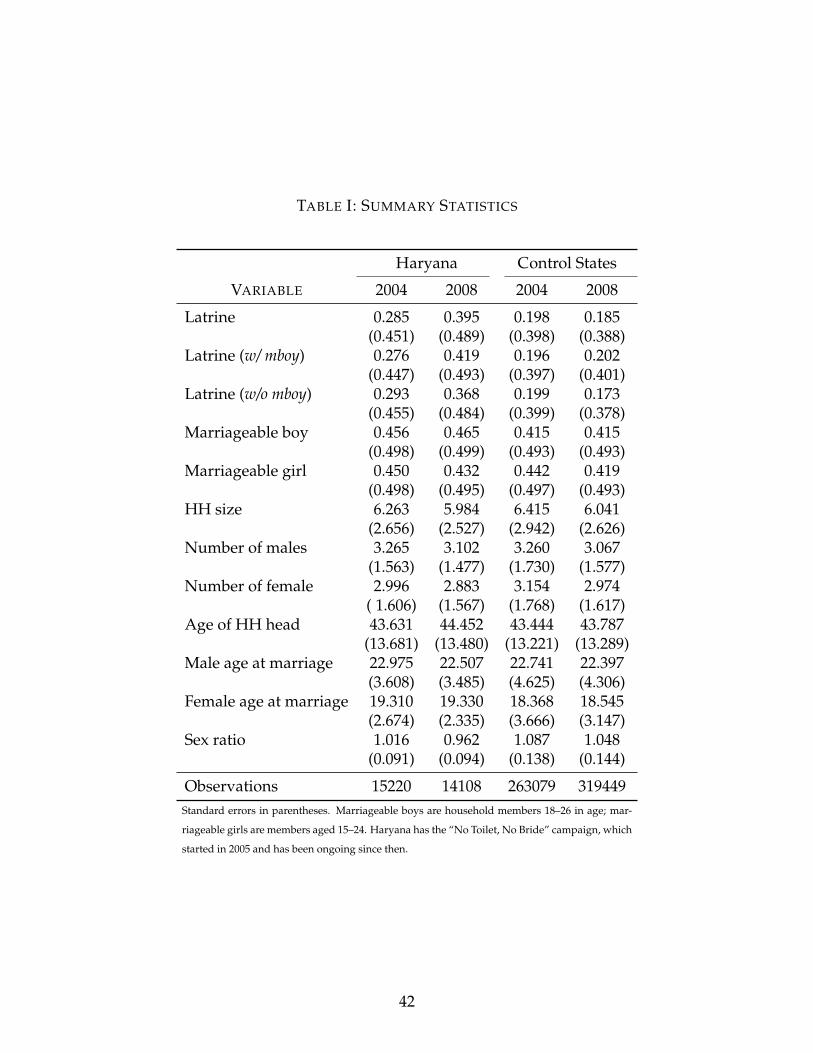
TABLE I: SUMMARY STATISTICS

Haryana Control States

VARIABLE 2004 2008 2004 2008

Latrine 0.285 0.395 0.198 0.185(0.451) (0.489) (0.398) (0.388)

Latrine (w/ mboy) 0.276 0.419 0.196 0.202(0.447) (0.493) (0.397) (0.401)

Latrine (w/o mboy) 0.293 0.368 0.199 0.173(0.455) (0.484) (0.399) (0.378)

Marriageable boy 0.456 0.465 0.415 0.415(0.498) (0.499) (0.493) (0.493)

Marriageable girl 0.450 0.432 0.442 0.419(0.498) (0.495) (0.497) (0.493)

HH size 6.263 5.984 6.415 6.041(2.656) (2.527) (2.942) (2.626)

Number of males 3.265 3.102 3.260 3.067(1.563) (1.477) (1.730) (1.577)

Number of female 2.996 2.883 3.154 2.974( 1.606) (1.567) (1.768) (1.617)

Age of HH head 43.631 44.452 43.444 43.787(13.681) (13.480) (13.221) (13.289)

Male age at marriage 22.975 22.507 22.741 22.397(3.608) (3.485) (4.625) (4.306)

Female age at marriage 19.310 19.330 18.368 18.545(2.674) (2.335) (3.666) (3.147)

Sex ratio 1.016 0.962 1.087 1.048(0.091) (0.094) (0.138) (0.144)

Observations 15220 14108 263079 319449Standard errors in parentheses. Marriageable boys are household members 18–26 in age; mar-

riageable girls are members aged 15–24. Haryana has the “No Toilet, No Bride” campaign, which

started in 2005 and has been ongoing since then.

42

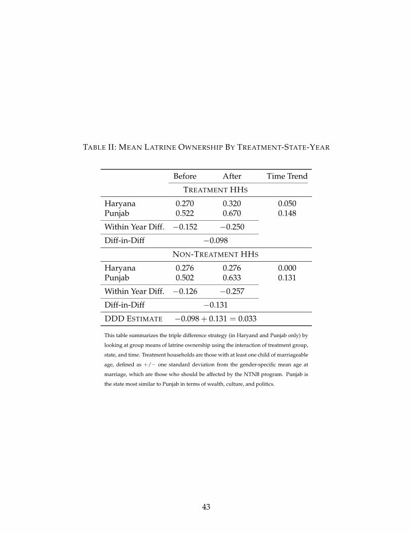
TABLE II: MEAN LATRINE OWNERSHIP BY TREATMENT-STATE-YEAR

Before After Time Trend

TREATMENT HHS

Haryana 0.270 0.320 0.050Punjab 0.522 0.670 0.148

Within Year Diff. −0.152 −0.250

Diff-in-Diff −0.098

NON-TREATMENT HHS

Haryana 0.276 0.276 0.000Punjab 0.502 0.633 0.131

Within Year Diff. −0.126 −0.257

Diff-in-Diff −0.131

DDD ESTIMATE −0.098 + 0.131 = 0.033

This table summarizes the triple difference strategy (in Haryand and Punjab only) by

looking at group means of latrine ownership using the interaction of treatment group,

state, and time. Treatment households are those with at least one child of marriageable

age, defined as +/− one standard deviation from the gender-specific mean age at

marriage, which are those who should be affected by the NTNB program. Punjab is

the state most similar to Punjab in terms of wealth, culture, and politics.

43

TABLE III: LATRINE ADOPTION (DIFF-IN-DIFF ESTIMATES)

Latrine (1) (2) (3) (4)

Mboy x Post 0.061∗∗∗ 0.057∗∗∗ 0.070∗∗∗ 0.038∗∗∗

(0.014) (0.011) (0.015) (0.012)Mboy -0.017 -0.041∗∗∗ 0.011 -0.039∗∗∗

(0.011) (0.007) (0.010) (0.010)Post 0.082∗∗∗ 0.065 0.015 0.039∗∗

(0.026) (0.017) (0.033) (0.019)Constant 0.276∗∗∗ -0.239∗∗∗ 0.362∗∗∗ -0.277∗∗∗

(0.026) (0.015) (0.034) (0.019)

Controls N Y N YR2 0.014 0.251 0.021 0.249N 29345 27815 29328 27815

The dependent variable is a dummy variable for whether household i has a la-

trine. Column (1) reports the basic DD regression using the mboy variable. Column

(2) adds the following control variables: age and education of the household head,

wife/mother’s education, household size, and four proxies for wealth (house type,

fan, TV, phone, and motorcycle). Column (3) using the fraction of mboys variable, which

uses total number of mboys in the household as a fraction of total children in order

to account for household fertility. Column (4) adds the same control variables to the

regression from Column (3). The primary coefficient of interest in all cases is the dou-

ble interaction. All standard errors are clustered at the village-year level. Significance

levels: ∗∗∗p< .01 ∗∗p< .05 ∗p< .1.

44

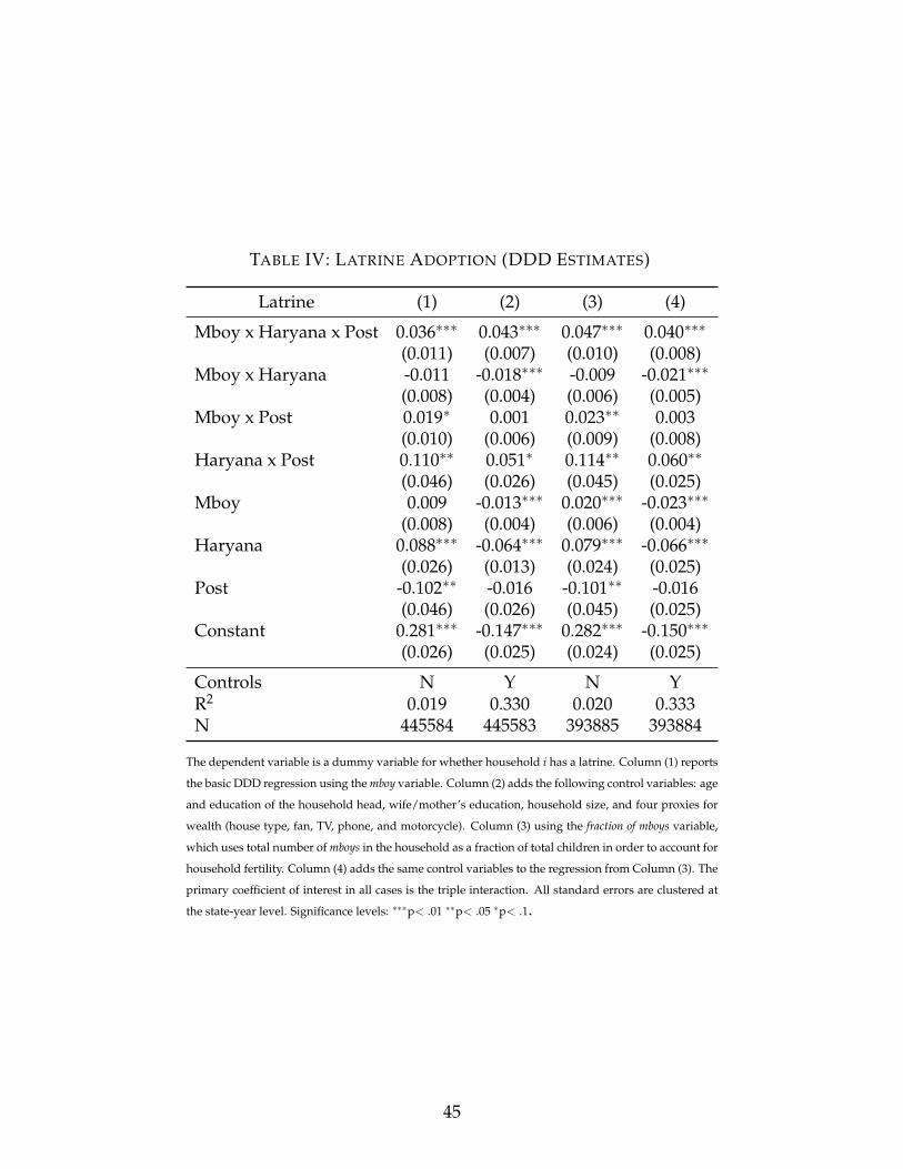
TABLE IV: LATRINE ADOPTION (DDD ESTIMATES)

Latrine (1) (2) (3) (4)

Mboy x Haryana x Post 0.036∗∗∗ 0.043∗∗∗ 0.047∗∗∗ 0.040∗∗∗

(0.011) (0.007) (0.010) (0.008)Mboy x Haryana -0.011 -0.018∗∗∗ -0.009 -0.021∗∗∗

(0.008) (0.004) (0.006) (0.005)Mboy x Post 0.019∗ 0.001 0.023∗∗ 0.003

(0.010) (0.006) (0.009) (0.008)Haryana x Post 0.110∗∗ 0.051∗ 0.114∗∗ 0.060∗∗

(0.046) (0.026) (0.045) (0.025)Mboy 0.009 -0.013∗∗∗ 0.020∗∗∗ -0.023∗∗∗

(0.008) (0.004) (0.006) (0.004)Haryana 0.088∗∗∗ -0.064∗∗∗ 0.079∗∗∗ -0.066∗∗∗

(0.026) (0.013) (0.024) (0.025)Post -0.102∗∗ -0.016 -0.101∗∗ -0.016

(0.046) (0.026) (0.045) (0.025)Constant 0.281∗∗∗ -0.147∗∗∗ 0.282∗∗∗ -0.150∗∗∗

(0.026) (0.025) (0.024) (0.025)

Controls N Y N YR2 0.019 0.330 0.020 0.333N 445584 445583 393885 393884

The dependent variable is a dummy variable for whether household i has a latrine. Column (1) reports

the basic DDD regression using the mboy variable. Column (2) adds the following control variables: age

and education of the household head, wife/mother’s education, household size, and four proxies for

wealth (house type, fan, TV, phone, and motorcycle). Column (3) using the fraction of mboys variable,

which uses total number of mboys in the household as a fraction of total children in order to account for

household fertility. Column (4) adds the same control variables to the regression from Column (3). The

primary coefficient of interest in all cases is the triple interaction. All standard errors are clustered at

the state-year level. Significance levels: ∗∗∗p< .01 ∗∗p< .05 ∗p< .1.

45

TABLE V: SEX RATIOS & MARRIAGE MARKET COMPETITION (DD ESTIMATES)

LOW SEX RATIO HIGH SEX RATIO

Latrine Ownership Coef. p-value Coef. p-value

Mboy x Post 0.075∗∗∗ 0.000 0.020 0.308(0.014) (0.019)

Mboy -0.022∗ 0.050 0.001 0.906(0.011) (0.012)

Post 0.133∗∗∗ 0.000 0.034∗∗∗ 0.009(0.020) (0.013)

Constant 0.241∗∗∗ 0.000 0.348∗∗∗ 0.000(0.000) (0.008)

R2 0.034 0.002N 18399 10568

The dependent variable is a dummy for whether household i owns a latrine. I run this specifica-

tion separately for households in a competitive marriage market (from the marriageable boy’s

perspective), which is defined as having more marriageable boys than marriageable girls, and

for households in a less competitive marriage market. These are the low and high sex ratio

columns, respectively. The coefficients of interest (the double interactions) are statistically dif-

ferent from each other at the 99% level. Standard errors, clustered at the village-year level, are

reported in parentheses. Significance levels: ∗∗∗p< .01 ∗∗p< .05 ∗p< .1

46

TABLE VI: SEX RATIOS & MARRIAGE MARKET COMPETITION (DDD ESTIMATES)

LOW SEX RATIO HIGH SEX RATIO

Latrine Ownership Coef. p-value Coef. p-value

Mboy x Haryana x Post 0.065∗∗∗ 0.007 0.018∗ 0.061(0.024) (0.009)

Mboy x Haryana -0.044∗∗ 0.038 -0.018 0.199(0.021) (0.014)

Mboy x Post 0.005∗ 0.443 0.036∗∗ 0.028(0.006) (0.015)

Haryana x Post 0.099∗ 0.056 -0.110∗∗∗ 0.007(0.042) (0.036)

Mboy 0.016∗∗∗ 0.002 0.007 0.611(0.004) (0.012)

Haryana 0.056 0.226 0.090∗∗ 0.018(0.046) (0.034)

Post 0.110∗∗∗ 0.000 -0.170∗∗∗ 0.000(0.021) (0.037)

Constant 0.136∗∗∗ 0.000 0.291∗∗∗ 0.000(0.010) (0.012)

R2 0.028 0.028N 249100 270938

The dependent variable is a dummy for whether household i owns a latrine. I run this specifica-

tion separately for households in a competitive marriage market (from the marriageable boy’s

perspective), which is defined as having more marriageable boys than marriageable girls, and

for households in a less competitive marriage market. These are the low and high sex ratio

columns, respectively. The coefficients of interest (the triple interactions) are statistically dif-

ferent from each other at the 99% level. Standard errors, clustered at the state-year level, are

reported in parentheses. Significance levels: ∗∗∗p< .01 ∗∗p< .05 ∗p< .1

47

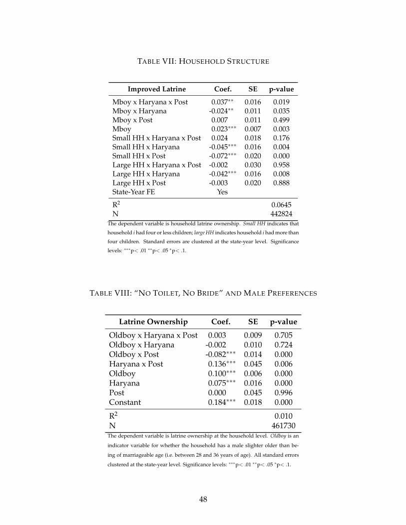
TABLE VII: HOUSEHOLD STRUCTURE

Improved Latrine Coef. SE p-value

Mboy x Haryana x Post 0.037∗∗ 0.016 0.019Mboy x Haryana -0.024∗∗ 0.011 0.035Mboy x Post 0.007 0.011 0.499Mboy 0.023∗∗∗ 0.007 0.003Small HH x Haryana x Post 0.024 0.018 0.176Small HH x Haryana -0.045∗∗∗ 0.016 0.004Small HH x Post -0.072∗∗∗ 0.020 0.000Large HH x Haryana x Post -0.002 0.030 0.958Large HH x Haryana -0.042∗∗∗ 0.016 0.008Large HH x Post -0.003 0.020 0.888State-Year FE Yes

R2 0.0645N 442824

The dependent variable is household latrine ownership. Small HH indicates that

household i had four or less children; large HH indicates household i had more than

four children. Standard errors are clustered at the state-year level. Significance

levels: ∗∗∗p< .01 ∗∗p< .05 ∗p< .1.

TABLE VIII: “NO TOILET, NO BRIDE” AND MALE PREFERENCES

Latrine Ownership Coef. SE p-value

Oldboy x Haryana x Post 0.003 0.009 0.705Oldboy x Haryana -0.002 0.010 0.724Oldboy x Post -0.082∗∗∗ 0.014 0.000Haryana x Post 0.136∗∗∗ 0.045 0.006Oldboy 0.100∗∗∗ 0.006 0.000Haryana 0.075∗∗∗ 0.016 0.000Post 0.000 0.045 0.996Constant 0.184∗∗∗ 0.018 0.000

R2 0.010N 461730

The dependent variable is latrine ownership at the household level. Oldboy is an

indicator variable for whether the household has a male slighter older than be-

ing of marriageable age (i.e. between 28 and 36 years of age). All standard errors

clustered at the state-year level. Significance levels: ∗∗∗p< .01 ∗∗p< .05 ∗p< .1.

48

TABLE IX: FEMALE PREFERENCES OUTSIDE OF MARRIAGE

Latrine Ownership Coef. SE p-value

Mgirl x Haryana x Post 0.005 0.011 0.669Mgirl x Haryana 0.020∗∗∗ 0.006 0.003Mgirl x Post -0.003 0.111 0.798Haryana x Post 0.115∗∗ 0.042 0.010Mgirl 0.022∗∗∗ 0.006 0.001Haryana 0.079∗∗∗ 0.018 0.000Post -0.015 0.042 0.724Constant 0.192∗∗∗ 0.018 0.000

R2 0.007N 455113Sample focuses on single mgirls only by excluding households with both

mboys and mgirls. All standard errors clustered at the state-year level. Sig-

nificance levels: ∗∗∗p< .01 ∗∗p< .05 ∗p< .1.

FIGURE II: MARRIAGE AND INVESTMENT INCENTIVES

θ

c

−Ul-Uh

φx

φx + Uh - Ul

InvestmentNo marriage

Marry but no investmentNo marriage, no investment

Always marry Never marry

The idiosyncratic gain to marriage, θ, is along the x-axis. Individual costs of investment are along the y-axis. The

yellow region indicates those men who will invest. Graph is adapted from Chiappori, Iyigun, and Weiss (2009).

49

TABLE X: FURTHER EVIDENCE ON INTRAHOUSEHOLD ALLOCATION

Dep. Var. Full Latrine No Latrine Diff.

Education gap 0.016 0.099∗ -0.032 0.131∗∗∗

(0.031) (0.050) (0.032)Age gap -0.012 0.026 -0.003 0.029

(0.053) (0.113) (0.956)Age at first birth 0.208∗∗ 0.105 0.188∗ -0.083

(0.091) (0.078) (0.098)Pregnant -0.013∗∗ -0.013∗ -0.007 -0.006

(0.006) (0.006) (0.007)Contraceptive use -0.027∗ -0.002 -0.022 -0.020

(0.014) (0.013) (0.170)Marriage age -0.042 0.163∗∗∗ -0.079 0.242∗∗∗

(0.064) (0.051) (0.073)Living with husband 0.145∗ 0.291∗∗∗ 0.013 0.278∗∗∗

(0.069) (0.049) (0.077)Sewing machine 0.035∗∗∗ 0.029∗∗ 0.021∗∗ 0.008

(0.008) (0.012) (0.008)Washing machine 0.022∗∗∗ 0.011∗∗ 0.017∗∗∗ -0.006

(0.002) (0.004) (0.001)Cooker -0.005 -0.003 0.003 0.006

(0.005) (0.006) (0.007)Fan 0.012 0.003 0.031 -0.028∗∗∗

(0.006) (0.008) (0.007)Television -0.014∗∗ -0.019 -0.023∗∗∗ -0.004

(0.005) (0.016) (0.007)Motorcycle 0.052∗∗∗ 0.049∗∗∗ 0.027∗∗∗ 0.022∗∗

(0.008) (0.018) (0.008)

Reported coefficients are from the triple interaction of mboy-haryana-post. The coefficients for mar-

riage age, age at which first living with husband, washing machine, and cooker are all based on the

difference-in-difference using mboy status and Haryana/control (i.e. with no time dimension) due to

variables being missing from the 2004 round. The first column reports the basic DDD or DD esti-

mates. Column “Diff” reports the statistical significance of the difference between the coefficients from

columns (2) and (3) based on p > χ2. All standard errors are clustered at the state-year level. Signifi-

cance levels: ∗∗∗p< .01 ∗∗p< .05 ∗p< .1.

50

References[1] ABRAMITZKY, RAN, ADELINE DELAVANDE, & LUIS VASCONCELOS, ‘Marrying Up: The Role

of Sex Ratio in Assortative Matching.’ American Economic Journal: Applied Economics, 3, pp. 124–157, July, 2011.

[2] ANGRIST, JOSH, ‘How do Sex Ratios Affect Marriage and Labor Markets? Evidence from Amer-ica’s Second Generation*.’ Quarterly Journal of Economics, 117 (3), pp. 997–1038, August, 2002.

[3] ARNOLD, FRED, SUNITA KISHOR, & TK ROY, ‘Sex Selection Abortion in India.’ Population andDevelopment Review, 28 (4), pp. 759–785, 2002.

[4] ARUNACHALAM, RAJ & SURESH NAIDU, ‘The Price of Fertility: Marriage Markets and FamilyPlanning in Bangladesh.’ Working Paper, November, 2006.

[5] BANERJEE, ABHIJIT, ESTHER DUFLO, MAITREESH GHATAK, & JEANNE LAFORTUNE, ‘Marryfor What: Caste and Mate Selection in Modern India.’ NBER Working Paper, 2009.

[6] BECKER, GARY S, ‘A Theory of Marriage: Part I.’ The Journal of Political Economy, 81 (4), pp.813–846, July, 1973.

[7] BHARADWAJ, PRASHANT & LEAH NELSON, ‘Discrimination Begins in the Womb: Evidence ofSex-Selective Prenatal Investments.’ Working Paper, October, 2010.

[8] BLACK, RE, SE MORRIS, & J BRYCE, ‘Where and Why Are 10 Million Children Dying EveryYear?’ Lancet, 361, pp. 2226–34, 2003.

[9] BLOCH, FRANCIS, VIJAYENDRA RAO, & SONALDE DESAI, ‘Wedding Celebrations as Conspic-uous Consumption: Signaling Social Status in Rural India.’ Journal of Human Resources, 39 (3),pp. 675–695, 2004.

[10] BROWNING, MARTIN & PIERRE-ANDRÉ CHIAPPORI, ‘Efficient Intra-Household Allocations: AGeneral Characterization and Empirical Tests.’ Econometrica, 66 (6), pp. 1241–1278, 1998.

[11] CHAKRABORTY, TANIKA & SUKKOO KIM, ‘Caste, Kinship, and Sex Ratios in India.’ NBERWorking Paper (13828), pp. 1–60. 2008.

[12] CHIAPPORI, PIERRE-ANDRÉ, BERNANRD FORTIN, & GUY LACROIX, ‘Marriage Market, Di-vorce Legislation, and Household Labor Supply.’ Journal of Political Economy, 110 (1), pp. 37–72,2002.

[13] , MURAT IYIGUN, & YORAM WEISS, ‘Investment in Schooling and the Marriage Market.’American Economic Review, 99 (5), pp. 1689–1713, December, 2009.

[14] DAS GUPTA, MONICA, ‘Selective Discrimination Against Female Children in Rural Punjab,India.’ Population and Development Review, 13 (1), pp. 77–100, 1987.

[15] DESAI, SONALDE & LESTER ANDRIST, ‘Gender Scripts and Age at Marriage in India.’ Demog-raphy, 47 (3), pp. 667–687, 2010.

[16] DUTT, ASHOK K, ALLEN G NOBLE, & SATISH K DAVGUN, ‘Socioeconomic Factors AffectingMarriage Distance in Two Sikh Villages of Punjab.’ Journal of Cultural Geography, 2 (1), pp. 13–26,1981.

51

[17] ESWARAN, MUKESH, BHARAT RAMASWAMI, & WILIMA WADHWA, ‘Status, Caste, and theTime Allocation of Women in Rural India.’ Working Paper, 2009.

[18] GALE, DAVID & LLOYD S SHAPLEY, ‘College Admissions and the Stability of Marriage.’ TheAmerican Mathematical Monthly, 69 (1), pp. 9–15, January, 1962.

[19] GOULD, HAROLD A, ‘A Further Note on Village Exogamy in North India.’ Southwestern Journalof Anthropology, 17 (3), pp. 297–300, 1961.

[20] IYIGUN, MURAT & RANDALL P WALSH, ‘Building the Family Nest: Premarital Investments,Marriage Markets, and Spousal Allocations.’ Review of Economic Studies, 74 (2), pp. 507–535,April, 2007.

[21] LAFORTUNE, JEANNE, ‘Making Yourself Attractive: Pre-Marital Investments and the Returnsto Education in the Marriage Market.’ Working Paper, pp. 1–49, September, 2010.

[22] MUNSHI, KAIVAN & MARK R ROSENZWEIG, ‘Traditional Institutions Meet the Modern World:Caste, Gender, and Schooling Choice in a Globalizing Economy.’ American Economic Review, 96(4), pp. 1225–1252, 2006.

[23] OSTER, EMILY & REBECCA THORNTON, ‘Menstruation, Sanitary Products, and School Atten-dance: Evidence from a Randomized Evaluation.’ American Economic Journal: Applied Economics,3 (1), pp. 91–100, 2011.

[24] PATIL, SUMEET & ALICIA SALVATORE, ‘India Impact Evaluation Baseline Survey: DescriptiveReport.’Technical report, Water and Sanitation Program of the World Bank, 2010.

[25] QIAN, NANCY, ‘Missing Women and the Price of Tea in China: The Effect of Sex-Specific Earn-ings on Sex Imbalance.’ Quarterly Journal of Economics, 123 (3), pp. 1251–1285, August, 2008.

[26] ROSENZWEIG, MARK R & ODED STARK, ‘Consumption Smoothing, Migration, and Marriage:Evidence from Rural India.’ Journal of Political Economy, 97 (4), pp. 905–926, January, 1989.

[27] SHAPLEY, LLOYD S & MARTIN SHUBIK, ‘The Assignment Game I: The Core.’ International Jour-nal of Game Theory, 1 (1), pp. 111–130, 1972.

[28] WORLD BANK, ‘Toolkit on Hygiene, Sanitation and Water in Schools: Gender Roles and Im-pact.’Technical report, Water and Sanitation Program of the World Bank, 2005.

52

(Adverse) General Equilibrium Effects

of Cash Transfers†

M. Christian Lehmann‡

September 2013

If general equilibrium effects are taken into account, cash transfers to eligible households indirectly de-crease utility of ineligible households living in the same neighborhood. A hike in local prices outweighsthe income effect from higher local wages. Households with low labor endowments are particularlyaffected. Our results contrast sharply with the common notion that this class of programs generatespositive multiplier effects on the local economy.

JEL Classification: E21, H43, I38, O12, O17Keywords: Policy evaluation, general equilibrium effects, structural estimation

†I am very grateful to Francois Bourguignon for his guidance. I further thank Martin Ravallion, Ken Wolpin,Jere Behrman, Alain de Janvry, Giaccomo de Giorgi, Miguel Szekely, Francisco Ferreira, Raquel Tsukada,Catherine Guirkinger, Phillipe de Vreyer, Marc Gurgand, Karen Marcours, and conference/seminar partici-pants at Columbia University, MIT, Univ. of Minnesota, Paris School of Economics for helpful comments andsuggestions. Financial support from Region Ile-de-France is gratefully acknowledged. All errors are mine.‡Correspondence: clehmann@unb.br

1

1 Introduction

The general notion in the existing literature is that welfare programs gener-ate positive spillover effects on the local neighborhood. Miguel and Kremer(2004) show that anti-worm treatment to some individuals - because of re-ducing disease transmission - generates large benefits for other individualsnot receiving the treatment. Kaboski and Townsend (2011) find Microfi-nance to increase local wages. Angelucci and De Giorgi (2009), Bobonisand Finan (2009) and Lalive and Cattaneo (2009) report positive effectsof Oportunidades, Mexico’s flagship conditional cash transfer program, onfood consumption and human capital investments of program-ineligiblehouseholds residing in the neighborhood.

The results presented in this paper contrast with this notion. When gen-eral equilibrium effects are taken into account, cash transfers indirectlydecrease utility of ineligible households living in the same neighborhood.

We study the effects of Oportunidades within a general equilibrium model.The model is simple in the sense that, unlike Todd and Wolpin (2006) andAttanasio et al. (2012), it is static and ignores fertility and educationalchoices. Instead, the model puts emphasis on equilibrium effects in factorand commodity markets. The basic set-up consists of a village populatedby poor and non-poor households. Each household is endowed with staple(food) as well as labor, and chooses a consumption bundle (food, non-food, leisure) which maximizes utility subject to a budget constraint. Poorhouseholds receive a social security cash payment by the federal govern-ment. The staple (food) is produced inside the village, while the non-foodcommodity is produced outside. The village exports a fraction of its stapleand imports non-food commodities. These assumptions reflect that ruralareas specialize in staple production, while importing industrialized prod-ucts from urban areas.1 Importing implies transactions costs, in particularlabor. The village price of non-food consists of an exogenous component(‘world market’ price) plus an endogenous component (labor costs linkedto importing non-food to the village). Labor costs are endogenous becausethe procurement of non-food requires village residents’ labor.2 In equilib-

1Household data for rural Mexico, for example, shows that half of rural households’ monthly con-sumption consists of imported hygiene products (e.g. soap, combs, tooth and hair brushes, detergents,whiteners), household utensils (plates, towels, combs etc.), clothing, tennis shoes and boots, schoolsupplies (pens and paper), and energy (batteries, gas, petrol).

2Major national grocery chains, or other forms of non-food procurement which do not require village

2

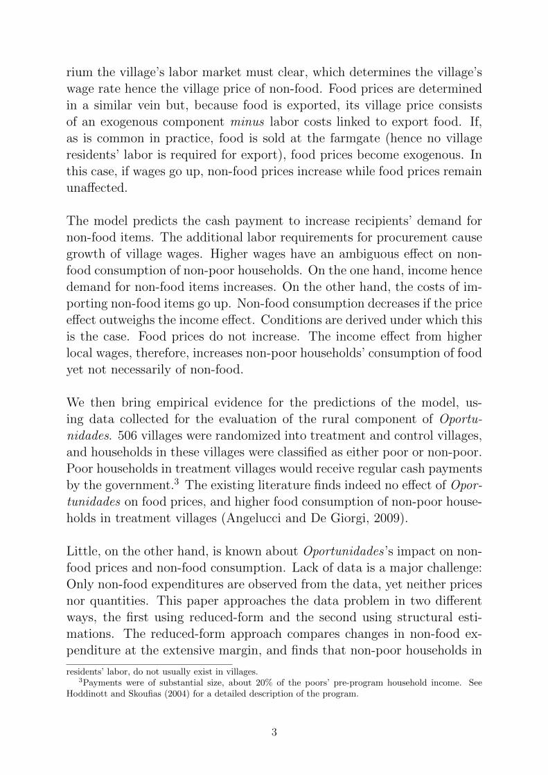
rium the village’s labor market must clear, which determines the village’swage rate hence the village price of non-food. Food prices are determinedin a similar vein but, because food is exported, its village price consistsof an exogenous component minus labor costs linked to export food. If,as is common in practice, food is sold at the farmgate (hence no villageresidents’ labor is required for export), food prices become exogenous. Inthis case, if wages go up, non-food prices increase while food prices remainunaffected.

The model predicts the cash payment to increase recipients’ demand fornon-food items. The additional labor requirements for procurement causegrowth of village wages. Higher wages have an ambiguous effect on non-food consumption of non-poor households. On the one hand, income hencedemand for non-food items increases. On the other hand, the costs of im-porting non-food items go up. Non-food consumption decreases if the priceeffect outweighs the income effect. Conditions are derived under which thisis the case. Food prices do not increase. The income effect from higherlocal wages, therefore, increases non-poor households’ consumption of foodyet not necessarily of non-food.

We then bring empirical evidence for the predictions of the model, us-ing data collected for the evaluation of the rural component of Oportu-nidades. 506 villages were randomized into treatment and control villages,and households in these villages were classified as either poor or non-poor.Poor households in treatment villages would receive regular cash paymentsby the government.3 The existing literature finds indeed no effect of Opor-tunidades on food prices, and higher food consumption of non-poor house-holds in treatment villages (Angelucci and De Giorgi, 2009).

Little, on the other hand, is known about Oportunidades ’s impact on non-food prices and non-food consumption. Lack of data is a major challenge:Only non-food expenditures are observed from the data, yet neither pricesnor quantities. This paper approaches the data problem in two differentways, the first using reduced-form and the second using structural esti-mations. The reduced-form approach compares changes in non-food ex-penditure at the extensive margin, and finds that non-poor households in

residents’ labor, do not usually exist in villages.3Payments were of substantial size, about 20% of the poors’ pre-program household income. See

Hoddinott and Skoufias (2004) for a detailed description of the program.

3

treatment villages have a lower probability of purchasing non-food items,suggesting a decrease in non-food consumption.

The structural approach uses an empirical version of the model - calibratedto the Oportunidades data - to simulate changes in consumed non-foodquantities. In a first step, the parameters of the model are calibrated todata available on households residing in control villages. In a second step,out-of-sample forecasts are conducted: The cash transfer is added to theincome of poor households in the control village sample. To test the per-formance of the model, the resulting simulated moments are compared tothe actual moments observed in the treatment village sample. Thus, inthe vein of Todd and Wolpin (2006), the experimental design of Opor-tunidades is used as a source of model validation. The model is able toreplicate reasonably well the moments of the treatment group sample. Thisincreases confidence in by the model simulated impacts of Oportunidadeson non-food consumption. The exercise suggests a decrease in non-poorhouseholds’ non-food consumption of about seven percent. Overall, utilityof the average non-poor household falls by roughly two percent.

Lastly, we study heterogenous effects on non-poor households’ per capitanon-food consumption. Analytical expressions are derived which show howthe sign and magnitude of the effect depend on household level parame-ters (endowments, preferences), as well as parameters that describe theprogram (size of cash payments) and local context (number of paymentrecipients, land distribution, aggregate agricultural productivity). Modeland the data, for example, suggest that non-food consumption and utilityare more likely to decrease in non-poor households with few labor endow-ments, i.e. in households with below average number of adult householdmembers.

2 Theory

A. The model

Consider a village populated by g = 2 groups of households: poorer house-holds (Ps) and somewhat richer households (Rs)

g ∈ P,R

4

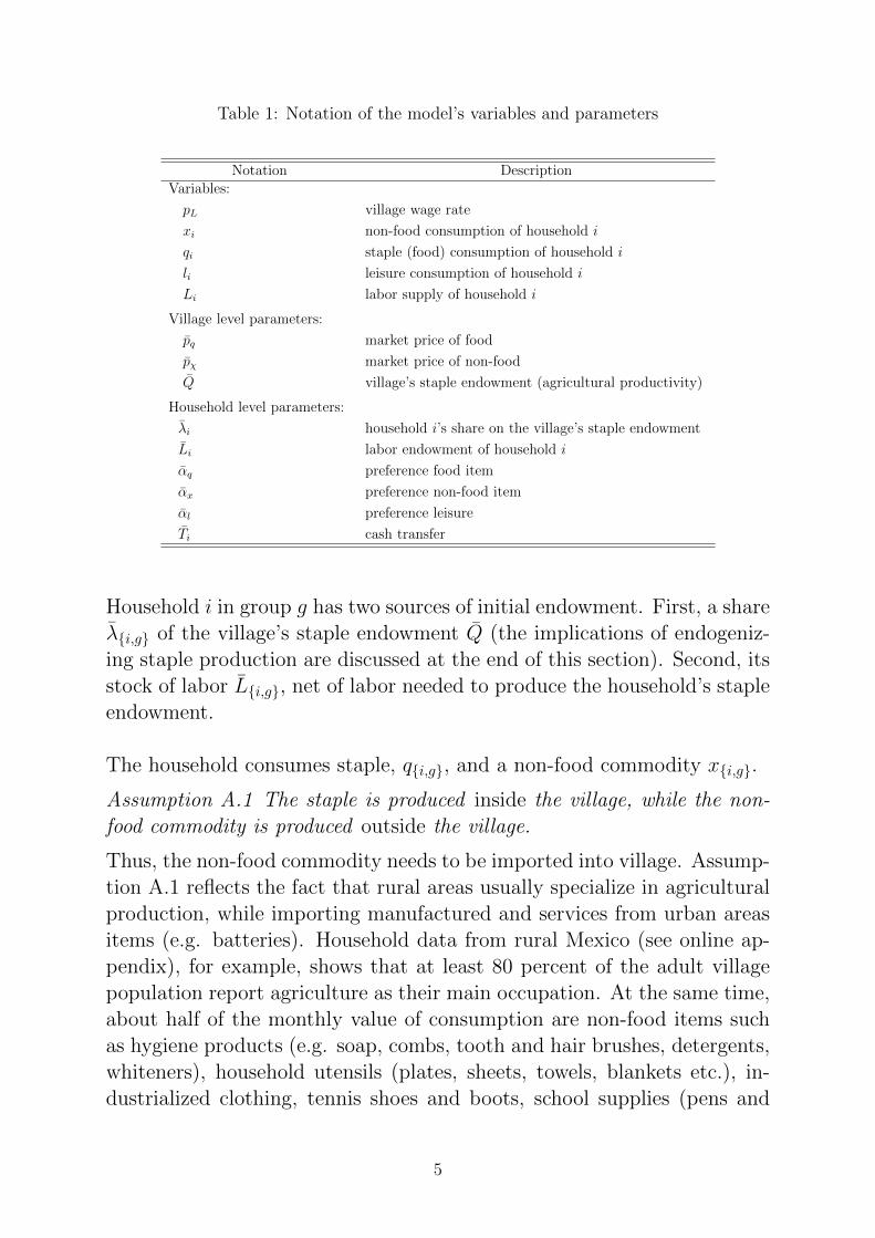
Table 1: Notation of the model’s variables and parameters

Notation DescriptionVariables:

pL village wage rate

xi non-food consumption of household i

qi staple (food) consumption of household i

li leisure consumption of household i

Li labor supply of household i

Village level parameters:

pq market price of food

pχ market price of non-food

Q village’s staple endowment (agricultural productivity)

Household level parameters:

λi household i’s share on the village’s staple endowment

Li labor endowment of household i

αq preference food item

αx preference non-food item

αl preference leisure

Ti cash transfer

Household i in group g has two sources of initial endowment. First, a shareλi,g of the village’s staple endowment Q (the implications of endogeniz-ing staple production are discussed at the end of this section). Second, itsstock of labor Li,g, net of labor needed to produce the household’s stapleendowment.

The household consumes staple, qi,g, and a non-food commodity xi,g.

Assumption A.1 The staple is produced inside the village, while the non-food commodity is produced outside the village.

Thus, the non-food commodity needs to be imported into village. Assump-tion A.1 reflects the fact that rural areas usually specialize in agriculturalproduction, while importing manufactured and services from urban areasitems (e.g. batteries). Household data from rural Mexico (see online ap-pendix), for example, shows that at least 80 percent of the adult villagepopulation report agriculture as their main occupation. At the same time,about half of the monthly value of consumption are non-food items suchas hygiene products (e.g. soap, combs, tooth and hair brushes, detergents,whiteners), household utensils (plates, sheets, towels, blankets etc.), in-dustrialized clothing, tennis shoes and boots, school supplies (pens and

5

paper), and energy (batteries, gas, petrol). Given the latters’ industri-alized nature and the aforementioned high share of labor force employedin agriculture, these non-food items are unlikely to be produced by thevillage. Importing these items implies transactions costs:

Assumption A.2 For each unit of consumption of x it is required one unitof labor.

The village price of x is consequently px = pχ +pL, where pχ is the factoryprice of x and pL being the price of labor. The interpretation of x is notnecessarily limited to consumption of imported non-food commodities. Itcan also be thought of as a consumed service. Think of, for example, acarpenter service: In this case pχ may be the remuneration of the woodand tools that the carpenter is using, and pL the remuneration of the car-penter’s labor.

Assumption A.3 Utilities are comparable between households, and eachhousehold maximizes a utility function that represents its reflexive, transi-tive, complete, continuous, and convex preferences.

The utility function of i writes ui,g(qi,g, xi,g, li,g) where li,g is con-sumption of leisure.

Assumption A.4 All agents treat prices as parametric, and no trade is per-mitted to take place except at equilibrium prices.

Household i chooses a consumption bundle qi,g, xi,g, li,g which max-imizes its utility function subject to the household’s budget constraint:

maxqi,g,xi,g,li,g

ui,g(qi,g, xi,g, li,g) s.t.

px × xi,g + pq × qi,g ≡ [Li,g − li,g]pL + [λi,g × Q]pq + Ti,g

where Ti,g is a cash transfer granted by the government exclusively tog ∈ P, i.e. Ti,P > 0 and Ti,R = 0. Under the maintained assumption ofstrict quasi concavity of the utility function, the solution of the household’smaximization problem will result in a demand function for the food item

qi,g : (pL, Ti,g,Ω)→ <

the non-food item

xi,g : (pL, Ti,g,Ω)→ <

6

and a labor supply function (Li,g = L− li,g)

Li,g : (pL, Ti,g,Ω)→ <

as functions of the village’s wage rate (pL), the parameter vector Ω=pχ,pq, Li,g, λi,g, Q, and the cash transfer Ti,g.

B. Predictions

Lets first consider the benchmark case in which there are no local generalequilibrium effects (pL is exogenous).

PROPOSITION 2.1 Under assumptions A.1-A.4, we have that∂xi,P/∂Ti,P > 0 and ∂qi,P/∂Ti,P > 0. For g ∈ R, however,∂qi,R/∂Ti,P = xi,R/∂Ti,P = 0.

Proof. A utility function which fulfills the preference requirements of as-sumption A.2 is the Cobb-Douglas utility function4

ui,g(qi,g, xi,g, li,g) = qαqi x

αxi l

1−αq−αxi with 0 < αq + αx < 1.

Utility maximization then yields demand and labor supply functions ofthe form

qi,g = αq[L× pL + λi,g × Q× pq + Ti,g]/pq (1)

xi,g = αx[L× pL + λi,g × Q× pq + Ti,g]/[pχ + pL] (2)

Li,g = Li,g − [1− αq − αx][L× pL + λi,g × Q× pq + Ti,g]/pL(3)

Deriving with respect to Ti,P yields ∂qi,P/∂Ti,P = αq/pq > 0, and∂xi,P/∂Ti,P = αx/[pχ + pL] > 0, and ∂Li,P/∂Ti,P = −[1 − αq −αx]/pL < 0. For g ∈ R we have ∂xi,R/∂Ti,P = ∂qi,R/∂Ti,P = 0 and∂Li,R/∂Ti,P = 0.

The cash transfer generates a positive income effect for g ∈ P. Demandfor qi,P, xi,P and li,P increases.

The income effect for g ∈ R is zero and, consequently, demand remains un-changed. Existing empirical evidence, however, rejects these predictions.Angelucci and De Giorgi (2009), for example, show that food consumption

4Proposition 2.1, however, holds for every other utility function which fulfils the preference require-ments of A.2.

7

of non-poor households increases.

Now, lets allow for local general equilibrium effects. The village’s labormarket equilibrium writes∑

g

∑i

Li,g ≡∑g

∑i

xi,g (4)

where the left hand side is the village’s aggregate labor supply. By as-sumption A.2, the right hand side is the village’s aggregate labor demand.Equation (4) assumes that the village labor market is local (i.e. limited tothe village’s population). This assumption is corroborated by, first, datafrom the 2002 Encuesta Nacional de Hogares Rurales (a representativehousehold survey of rural Mexico), where only six percent of adult vil-lage residents report to do non-agricultural work in a different village. Weare not aware of any studies looking at cross-village migration in Mexico.Existing studies exploit the Mexican census, where respondents are askedthe state in which they were born. It is however difficult to conclude fromcross-state migration about cross-village migration, because it is unclearto which extent cross-state migration simply reflects rural-to-urban migra-tion. But several factors suggest the magnitude of cross-village migrationto be rather low. First, land markets are often imperfect, which may con-strain the acquisition of land of emigrants (Finan et al., 2005). Second,formal credit and insurance markets are imperfect and informal insurancenetworks within the village a dominant source of insurance (Fafchampsand Lund, 2003). Thus, emigration is costly, because it may disconnectemigrants from these networks.

Second, there are usually no large supermarket/retail chains (which receiveproducts from its urban area headquarters) in rural villages. This impliesthat village residents’ labor is needed to import non-food (industrialized)products from urban areas.

PROPOSITION 2.2 (Endogenous wages) Under assumptions A.1-A.4, ∂qi,R/∂Ti,P > 0. However, ∂xi,R/∂Ti,P > 0 only if (1)labor endowment of i ∈ R is sufficiently large, or (2) stapleendowment of i ∈ R is sufficiently low.

8

Proof. Substituting (2) and (3) into (4) and solving for pL yields

p∗L =pχ[(αx − 1)(Q× pq +

∑i Ti,P)]∑

i Ti,P + Q× pq − αxpχ∑

g

∑i Li,g

. (5)

Note that the equilibrium wage is positive only if

Assumption A.5: αx∑

g

∑i Li,g > [

∑i Ti,P + Q× pq]/pχ,

i.e. if the village’s aggregate labor endowment is large enough to allow thevillage’s aggregate consumption demand for x to be satisfied. Substituting(5) into (1) and deriving with respect to Ti,P yields ∂qi,R/∂Ti,P > 0.Substituting (5) into (2) and deriving with respect to TP yields

∂xi,R

∂Ti,P=

[Li,Rpχ − λi,RQpq][αx − 1]∑

g

∑i Li,g

−(∑

g

∑i Li,gpχ − Qpq −

∑i Ti,P)

2(6)

By assumption A.5 the denominator in equation (6) is always negative.Since αx < 1, the term [αx − 1] in the numerator is always negative.Consequently, the sign of ∂xi,R/∂Ti,P will depend on the sign of thefirst term in brackets in the numerator. We have that

∂xi,R

∂Ti,P> 0 if Li,R/λi,RQ > pq/pχ. (7)

The intuition behind proposition 2.2 is the following: The cash grant in-creases cash recipients’ demand for non-food items. Importation of theseitems requires labor. The village’s labor demand increases, raising thevillage’s equilibrium wage.5 A higher wage, however, has an a priori am-biguous effect on non-food consumption of the remainder of the villagepopulation not receiving cash transfers. On the one hand, higher wagesimply a positive income effect which ceteris paribus increases consumptionof non-food items. On the other hand, because px = pχ + pL, higher wagesraise the village price of these non-food items, making their consumptionmore expensive. Non-food consumption of non-poor households decreasesif the price effect outweighs the income effect. Whether this is the case, ac-cording to condition (7), depends on a non-poor household’s endowments.In section 5 we will discuss in detail the crucial role of endowments.

5

∂p∗L∂Ti,P

=αx[αx − 1]p2χ

∑g

∑i Li,g

−[α∑g

∑i Li,gpχ −

∑i Ti,P − Q× pq]2

> 0

9

C. Discussion

The model is simple in that there is no credit and insurance market, andschooling conditionalities that come with Oportunidades are disregarded.Furthermore, the model does not allow for changes in agricultural pro-duction, and assumes away transaction costs for staple exports. In thefollowing we discuss the implication of these omissions.

(i.) School enrollment, classroom attendance, and social interactionsHigher payments are made to households that send their children to school.Paul Schultz (2004) finds a significant impact of Oportunidades on schoolenrollment and school attendance. In our model, school enrollment can beinterpreted, at least in the short term, a as reduction in a household’s netlabor endowment. Consider the stylized case where the loss of child incomecorresponds exactly to the value of the Oportunidades payment. In thiscase, a poor household’s budget constraint does not change. Demand forfood, non-food, and leisure remains unaffected, but labor supply decreases.Lower labor supply drives up equilibrium wages. As in proposition 2.2, fornon-poor households, higher wages imply an increase in food consumptionbut not necessarily in non-food consumption.

Bobonis and Finan (2009) and Lalive and Cattaneo (2009) find that, due topeer effects and social interactions inside the village, Oportunidades alsoincrease school enrollment of non-poor households residing in the sameneighborhood. If non-poor households enroll their children in school, theincome effect from higher local wages will be lower.

(ii.) Risk sharingAngelucci and De Giorgi (2009) find poor households to partially sharethe Oportunidades payment with their extended family. This would in-crease non-poor households’ income, on top of the increase in wages. Theeffect on food consumption would be higher, and a decrease in non-foodconsumption less likely.

(iii.) Exogenous vs. endogenous agricultural production, and farmgatesellingExogenous staple production may be a reasonable assumption in the shortbut not the long-run. The implications of endogenizing staple productionwill depend on assumptions about the agricultural market. First, con-

10

sider the standard separable agricultural household model setting (Singhet al., 1986), with a perfect village labor market, no transaction costs forselling staple, and a surplus-producing village, i.e. exogenous agriculturalprices. The increase in local wages resulting from the presence of Oportu-nidades would cause agricultural production to fall. Second, consider thecase where the village is not producing a surplus. The price of the staplebecomes endogenous. Higher demand exhibits upward pressure on priceswhich, ceteris paribus, increases production. Agricultural production fallsif higher wages outweigh the price effect. Third, in the case of transactioncosts for exporting the staple, higher wages imply a decrease in a farmer’sselling price hence production.

Should agricultural production fall, this would dampen the income effectfrom higher wages. Consequently, the increase in non-poor households’food consumption would be smaller, and a decrease in non-food consump-tion even more likely.

On the other hand, some non-poor household may be credit constrainedand invest additional wage income into agricultural production (Gertleret al., 2012; Bianchi and Bobba, 2013). In this case, the increase in foodconsumption would be higher, and a decrease in non-food consumptionless likely.

The model assumes that there are no transaction costs for exporting staple.Fafchamps and Hill (2005) show that farmgate selling is the most commonselling method of farmers in Uganda. For Mexico, we are not aware of anyquantitative study that documents the most common selling method offarmers. In field work the author conducted in about twenty Oportunidadesvillages, farmers reported to sell their harvest directly to a crop merchantwho visits the village with a truck after harvest. This suggests smalltransaction costs for farmers to sell their produce. There may, however, bevillages or regions were, for some reason, farmgate selling is not common.In this case, farmers need to transport their produce to the next regionalmarket. If labor is the only source of transaction costs - and assuming, forease of exposition, that the export of one unit of staple requires one unit ofthe village’s labor - then the village price of staple is pq = pQ − pL, wherepQ is the exogenous market price of staple. If a non-poor household is abuyer of staple then transaction costs for food exports do further reinforcethe increase in food consumption, because higher wages reduce the price

11

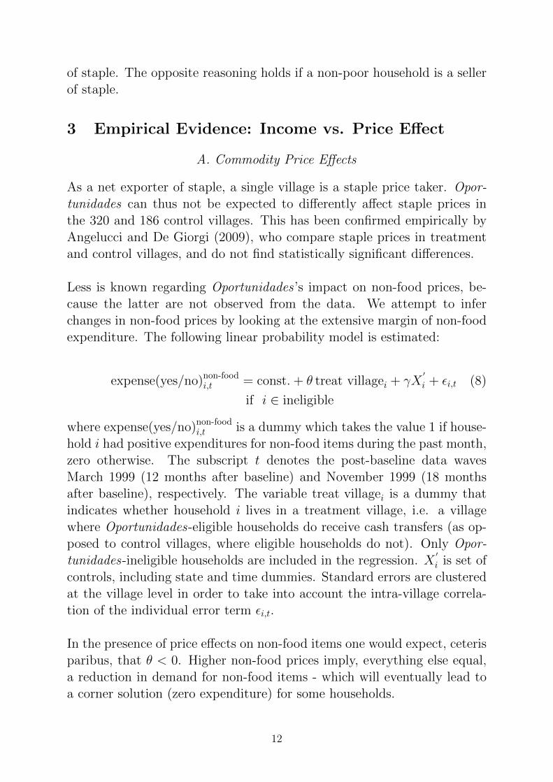
of staple. The opposite reasoning holds if a non-poor household is a sellerof staple.

3 Empirical Evidence: Income vs. Price Effect

A. Commodity Price Effects

As a net exporter of staple, a single village is a staple price taker. Opor-tunidades can thus not be expected to differently affect staple prices inthe 320 and 186 control villages. This has been confirmed empirically byAngelucci and De Giorgi (2009), who compare staple prices in treatmentand control villages, and do not find statistically significant differences.

Less is known regarding Oportunidades ’s impact on non-food prices, be-cause the latter are not observed from the data. We attempt to inferchanges in non-food prices by looking at the extensive margin of non-foodexpenditure. The following linear probability model is estimated:

expense(yes/no)non-foodi,t = const. + θ treat villagei + γX

′

i + εi,t (8)

if i ∈ ineligible

where expense(yes/no)non-foodi,t is a dummy which takes the value 1 if house-

hold i had positive expenditures for non-food items during the past month,zero otherwise. The subscript t denotes the post-baseline data wavesMarch 1999 (12 months after baseline) and November 1999 (18 monthsafter baseline), respectively. The variable treat villagei is a dummy thatindicates whether household i lives in a treatment village, i.e. a villagewhere Oportunidades-eligible households do receive cash transfers (as op-posed to control villages, where eligible households do not). Only Opor-tunidades-ineligible households are included in the regression. X

′

i is set ofcontrols, including state and time dummies. Standard errors are clusteredat the village level in order to take into account the intra-village correla-tion of the individual error term εi,t.

In the presence of price effects on non-food items one would expect, ceterisparibus, that θ < 0. Higher non-food prices imply, everything else equal,a reduction in demand for non-food items - which will eventually lead toa corner solution (zero expenditure) for some households.

12

Table 2 displays the OLS estimates of the linear probability model in equa-tion (8). The first column shows that Oportunidades-ineligible householdsin treatment villages are significantly more likely to have zero non-foodexpenditure. From column (2) to (5), which break down the result bynon-food category, we conclude that the effect reported in column (1) ismainly driven by a reduction in expenditure of hygiene and householdssupply products. This may be seen as additional evidence for the modelof section 2, which predicts price hikes for items which a village imports.Hygiene products (e.g. soap, shampoo, etc.) and households supplies (e.g.detergents) are typical examples of items that are not produced by thevillage, but which have to be imported from outside the village.

A note on identification: Behrman and Todd (1999) show treatment andcontrol group samples to be balanced at baseline, and Angelucci andDe Giorgi (2009) report no differential attrition rates. In terms of mea-surement error, ineligible households in treatment villages may underre-port their expenditure in order to appear eligible for Oportunidades. Ifthis would be true then one should expect ineligibles’ reported non-foodexpenditure to be lower in treatment villages. This, however, is not thecase.

B. Income Effect

Previous studies have estimated the impact of Oportunidades on wages.Angelucci and De Giorgi (2009) report no changes in wages. Their wagemeasure, however, include all sources sources of labor supply, includingagricultural wage labor. Because agricultural wage labor constitutes alarge share of total hours worked, yet largely being seasonal work on somecommercial farm away from the village, these wage measures are not likelyto capture the village’s wage rate.

We construct a wage proxy which is based on economic activities thatoccur inside the village. Our wage proxy, ω, is calculated as the sum ofreported daily profits from within-village activities (e.g. petty sales, tai-loring, washing and ironing, etc.). It is then checked whether this wageproxy, ωi, is different between treatment and control villages. The follow-ing model is estimated:

13

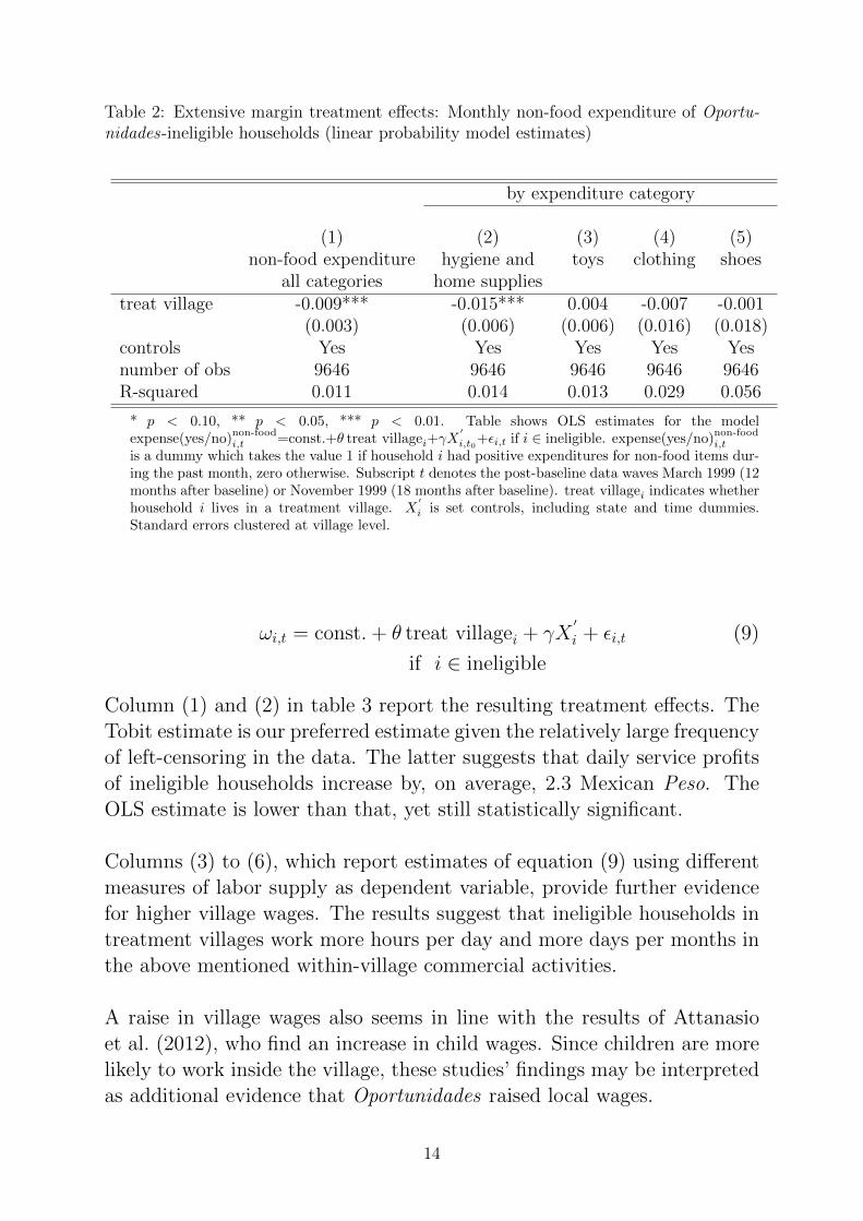
Table 2: Extensive margin treatment effects: Monthly non-food expenditure of Oportu-nidades-ineligible households (linear probability model estimates)

by expenditure category

(1) (2) (3) (4) (5)non-food expenditure hygiene and toys clothing shoes

all categories home suppliestreat village -0.009*** -0.015*** 0.004 -0.007 -0.001

(0.003) (0.006) (0.006) (0.016) (0.018)controls Yes Yes Yes Yes Yesnumber of obs 9646 9646 9646 9646 9646R-squared 0.011 0.014 0.013 0.029 0.056

* p < 0.10, ** p < 0.05, *** p < 0.01. Table shows OLS estimates for the modelexpense(yes/no)

non-foodi,t =const.+θ treat villagei+γX

′

i,t0+εi,t if i ∈ ineligible. expense(yes/no)

non-foodi,t

is a dummy which takes the value 1 if household i had positive expenditures for non-food items dur-ing the past month, zero otherwise. Subscript t denotes the post-baseline data waves March 1999 (12months after baseline) or November 1999 (18 months after baseline). treat villagei indicates whetherhousehold i lives in a treatment village. X

′

i is set controls, including state and time dummies.Standard errors clustered at village level.

ωi,t = const. + θ treat villagei + γX′

i + εi,t (9)

if i ∈ ineligible

Column (1) and (2) in table 3 report the resulting treatment effects. TheTobit estimate is our preferred estimate given the relatively large frequencyof left-censoring in the data. The latter suggests that daily service profitsof ineligible households increase by, on average, 2.3 Mexican Peso. TheOLS estimate is lower than that, yet still statistically significant.

Columns (3) to (6), which report estimates of equation (9) using differentmeasures of labor supply as dependent variable, provide further evidencefor higher village wages. The results suggest that ineligible households intreatment villages work more hours per day and more days per months inthe above mentioned within-village commercial activities.

A raise in village wages also seems in line with the results of Attanasioet al. (2012), who find an increase in child wages. Since children are morelikely to work inside the village, these studies’ findings may be interpretedas additional evidence that Oportunidades raised local wages.

14

Table 3: Treatment effect on Oportunidades-ineligible households’ daily service profits

dependent variable:

daily income hours per day days per months(1) (2) (3) (4) (5) (6)

OLS Tobit OLS Tobit OLS Tobittreat village 0.098* 2.298** 0.034 1.080** 0.260 4.264**

(0.053) (0.920) (0.053) (0.519) (0.170) (1.906)

controls Yes Yes Yes Yes Yes Yes

number of obs 9511 9511 9529 9529 9553 9553

* p < 0.10, ** p < 0.05, *** p < 0.01. Table shows estimates of the modelxi,t=const.+θ treat villagei+γX

′

i+εi,t if i ∈ ineligible. In columns (1) and (2), the dependent variableis daily profits (past week average) made from non-agricultural within-village commercial activities(e.g. petty trade, tailoring, washing and ironing, etc.) of household i, measured in Mexican Peso.The exchange rate in 1999 was roughly 1 US Dollar=10 Mexican Peso. In columns (3) and (4), thedependent variable is a household’s daily hours worked (past week average) in these activities. Incolumns (5) and (6), the dependent variable is a household’s monthly days worked in these activ-ities. Subscript t denotes the post-baseline data waves March 1999 (12 months after baseline) orNovember 1999 (18 months after baseline). treat villagei indicates whether household i lives in atreatment village. Only Oportunidades-ineligible households are included in the regression. X

′

i isset of controls, including state and time dummies. Standard errors at the village level. The toppercentile of the dependent variable is excluded.

15

4 Effects on Consumption and Utility

A positive income effect - in the absence of a price effect on food - impliesa positive effect of Oportunidades on food consumption of Oportunidades-ineligible households. That Oportunidades has indeed had a positive effecton food consumption of ineligible households is documented in Angelucciand De Giorgi (2009), who find positive treatment effects on food con-sumption of program-ineligible households.

Estimating Oportunidades ’s effect on non-food consumption of program-ineligible households is complicated by the fact that only non-food expen-diture is observed from the data, yet neither non-food prices nor quan-tities. In section 3, we have already provided some suggestive evidencethat Oportunidades may have lead to a decrease in non-food consumption:Oportunidades-ineligible households in treatment villages are significantlyless likely to have positive expenditure for non-food items (Table 2).

Another way of inferring changes in non-food quantities is by using anempirical version of the structural model introduced in section 2. In a firststep, we calibrate the parameters of the model to the data available onhouseholds residing in control villages. In a second step, we conduct out-of-sample forecasts: The cash transfer is added to the income of eligiblehouseholds in the control village sample. In order to test the performanceof the model, we compare the resulting simulated moments to the actualmoments observed in the treatment village sample. Thus, as in Toddand Wolpin (2006), we use the experimental design of Oportunidades as asource of model validation. The model is able to replicate quite well themoments of the treatment village sample. This increases our confidence inby the model simulated impacts of Oportunidades on non-food consump-tion. Next, we are going to describe these steps in greater detail.

A. Model equations

The model described in section 2 can be written as a set of nine equations:

Household full income is given by

IP = LP × pL + QP × pq + TP

IR = LR × pL + QR × pq

16

Where IP and IR denote the full income of the average Oportunidades-eligible (Poor) and Oportunidades-ineligible (Rich) household, respectively.LP and LR are labor endowments, QP and QR are staple endowments, TPis the Oportunidades cash transfer, pL and pq denote the village wage rateand staple price, respectively.Labor supply is given by

LP = LP − αl × IP/pLLR = LR − αl × IR/pL,

where αl is the Cobb-Douglas preference for leisure.Demand for non-food items is given by

xP = αx × IP/pxxR = αx × IR/px,

with px = pχ + m × pL. pχ is the factory price of non-food items. m

describes how many units of labor are needed to import one unit of thenon-food item. αx is the Cobb-Douglas preference for non-food items.Demand for food-items is given by

qP = αq × IP/pqqR = αq × IR/pq,

where αq is the Cobb-Douglas preference for food.A village’s labor market equilibrium is given by

(nP × xP + nR × xR)m = nP × LP + nR × LR,

where nP and nR denote the number of Oportunidades-eligible and Opor-tunidades-ineligible village residents, respectively.

B. Calibration

We calibrate the model exploiting data available on the control group ofthe Oportunidades randomized control trial (March 1999 data wave). Thevector of model parameters is:

Ω = pχ, pq, Li, Qi, αq, αx, m, ni i ∈ P,R

In Mexico, the staple is corn. 78 percent of households in the controlgroup cite corn as their main cultivated crop. Corn is also the domi-nant ingredient in the food consumption basket of Mexicans. A value for

17

Table 4: Parameter values

average eligible HH average ineligible HHVillage level parameters

price of food commodity (pq) 1.8

price of non-food commodity (pχ) 0.1

number of eligible households (nP ) 35.3

number of ineligible households (nR) 8.8

labor requirement per unit of x (m) 2.7

Household level parameters

food item endowment (Qi) 301.1 481.2

HH efficient units of labor (Li) 93.0 63.1

preference food item (αq) 0.512 0.512

preference non-food item (αx) 0.415 0.415

preference leisure (αl) 0.074 0.074

the market price of corn (pq) can be observed directly from administra-tive records (Ministry of Agriculture). Monthly corn production (in kilo-gram) of the average Oportunidades-eligible household in the control group(which amounts to roughly 300kg) is taken for QP . In an analog man-ner, monthly corn production (in kilogram) of the average Oportunidades-ineligible household in the control group (which amounts to roughly 450kg)is taken for QR. The number of eligible households in the average controlvillage, nP , is 35.3. The number of ineligible households in the averagecontrol village, nR, is 8.8.

Values for the following parameters can neither be obtained from admin-istrative records nor from the Oportunidades RCT data:

Λ = pχ, Li, αq, αx, m i ∈ P,R

In order to obtain values for these parameters, we exploit that some ofthe model’s endogenous variables, such as food consumption, non-foodexpenditure, and labor supply, are observed from the control group data.Denote this vector

YRCTC = qRCTi , (px × xi)RCT , LRCTi

where the RCT superscript (randomized control trial) and C subscriptis used to indicate sample averages of the Oportunidades control group.Denote Ysim(Λ) the vector of from the model simulated values of these

18

variables. We then calibrate Λ by minimizing the standardized squareddistance between YRCT

C and Ysim(Λ)

minΛE =

(YRCT

C −Ysim(Λ)

YRCTC

)2

The full calibration writes

minΛE =

∑i=P,R

(qRCTi − αq × Ii/pq

qRCTi

)2

+∑i=P,R

((px × xi)RCT − px × xi

(px × xi)RCT

)2

+∑i=P,R

(LRCTi − [Li − αl × Ii/pL]

LRCTi

)2

s.t.

px = pχ + m× pLIi = L× pL + Qi × pq + Ti

xi = αx × Ii/px(nRCTP × xRCTP + nRCTR × xRCTR )m = nRCTP × LRCTP + nRCTR × LRCTR

1 = αx + αq + αl

where i ∈ P,R. Table 4 shows all the parameter values of the model.

C. Model predictions (out-of-sample forecasts)

Having obtained values for the parameters of the model, we then add thecash transfer to the income of the Oportunidades-eligible household incontrol villages, and solve the model. This yields a vector of (on controlvillages) simulated outcomes.

Formally, we compute the simulated treatment effect for some outcome Yjof household i, θsimi,j, as the difference between simulated control group,

Y simi,j|Ω,TP=0, and simulated treatment group, Y sim

i,j|Ω,TP>0.

θsimi,j = Y simi,j|Ω,TP>0 − Y sim

i,j|Ω,TP=0

The predictions of the model are shown in table 5. The model predicts anincrease in ineligibles’ monthly food consumption of roughly four percent.

19

Table 5: Structural estimation Oportunidades ’s consumption effects

Oportunidades-ineligible Households

(1) (2)

observed predicted

Panel I: Food consumption

control group mean (C) 756.85 731.08

treatment group mean (T ) 757.34 759.44

T − C 14.01 28.35(s.e) (11.16)

(T − C)/C 0.019 0.039

Panel II: Non-food expenditure [quantity]

control group mean (C) 679.00[n/a] 592.51[29.17]

treatment group mean (T ) 700.44[n/a] 615.49[27.09]

T − C 31.94[n/a] 22.98[-2.08](s.e) (24.68)

(T − C)/C 0.047[n/a] 0.039[-0.071]

The first row of column (1) in panel I and II show March 1999 sample means of household monthlyfood consumption (Mexican Peso value) and non-food expenditure (Mexican Peso value) of programineligible households living in treatment villages. In 1999, the exchange rate was roughly 1 USDollar=10 Mexican Peso. The second row of column (1) in panel I and II show March 1999 samplemeans of household monthly food consumption (Mexican Peso value) and non-food expenditure(Peso value) of program ineligible households living in control villages. The third row of column(1) in panel I and II shows the treatment effect (θ) obtained from the treatment effect regressionxi = const.+θtreat villagei+εi ∀ i ∈ ineligible, where xi is household monthly food consumption(panel I), and household monthly non-food expenditure (panel II), respectively. The fourth row ofcolumn (1) in panel I and II show the ratio of treatment effect (third row) over the control group mean(first row). Column (2) in panel I and II show the by the general equilibrium model simulated values.Values in [] are consumed quantities (non-food quantities are not observed from the Oportunidadesdata).

This compares to about two percent observed from the experimental data.The model predicts an increase in ineligibles’ monthly non-food consump-tion expenditure of 3.9 percent. This compares to 4.7 percent observedfrom the experimental data.

The model replicates reasonably well the actual treatment effects. This in-creases our confidence in the model’s simulated changes in non-food quan-tities. The model, however, predicts a decrease in non-food consumptionof about seven percent. Overall, non-poor neighbors’ utility falls by twopercent.

20

5 Heterogenous Effects

So far, the analysis has focused on average effects. In this section weturn to heterogenous effects. Proposition 2.2 states that the neighborhoodeffect is

1. decreasing in a household’s labor endowment, in the case of non-foodconsumption

2. not related to a household’s labor endowment, in the case of foodconsumption

In the model, this is because large-labor-endowment households have lowerper capita consumption, ceteris paribus, than low-labor-endowment house-holds. Therefore, if local wages and non-food prices increase, per capitanon-food consumption of the low-labor-endowment households will be moreadversely affected. To see this, consider a simple household demand func-tion for non-food, xi/Li = αxIi/px, with Ii = pLLi+pqλiQ and px = pχ+pL.The notation is the same as in section 2. In per capita terms, this demandfunction writes xi = xi/Li = αx[pLLi + pqλiQ]/[pχ + pL]Li. Deriving withrespect to pL yields

∂xi∂pL

=αx

pχ + pL− αx[pLLi + pqλiQ]

[pχ + pL]2Li.

It is easy to see that ∂xi/∂pL > 0 if Li →∞, and ∂xi/∂pL < 0 if Li → 0.

For per capita food consumption, we have ∂qi/∂pL = αq/pq. Thus, if localwages increase, per capita food consumption of low-labor-endowment andhigh-labor-endowment households should be equally affected.

In order to test these predictions, the following regression model is esti-mated:

expense pcapitanon-foodi,t = constant + θ1 treat villagei

+ θ2 treat villagei × hhsize small

+ αhhsize small + γX′

i,t0+ εi,t (10)

if i ∈ ineligible,

where expense pcapitanon-foodi,t is per capita monthly household non-food ex-

penditure. We are primarily interested in the regression coefficient on theinteraction effect treat villagei× hhsize small, where variable hhsize small

21

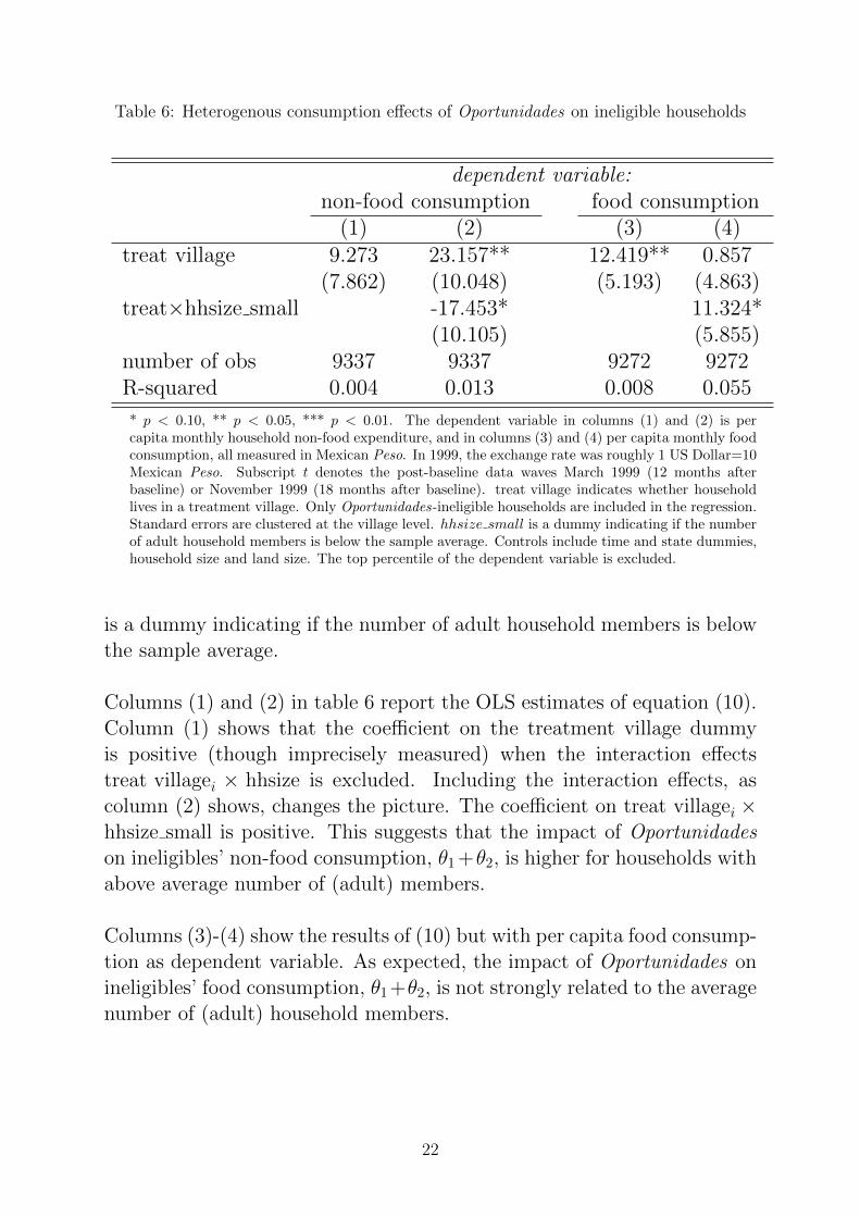
Table 6: Heterogenous consumption effects of Oportunidades on ineligible households

dependent variable:non-food consumption food consumption

(1) (2) (3) (4)treat village 9.273 23.157** 12.419** 0.857

(7.862) (10.048) (5.193) (4.863)treat×hhsize small -17.453* 11.324*

(10.105) (5.855)number of obs 9337 9337 9272 9272R-squared 0.004 0.013 0.008 0.055

* p < 0.10, ** p < 0.05, *** p < 0.01. The dependent variable in columns (1) and (2) is percapita monthly household non-food expenditure, and in columns (3) and (4) per capita monthly foodconsumption, all measured in Mexican Peso. In 1999, the exchange rate was roughly 1 US Dollar=10Mexican Peso. Subscript t denotes the post-baseline data waves March 1999 (12 months afterbaseline) or November 1999 (18 months after baseline). treat village indicates whether householdlives in a treatment village. Only Oportunidades-ineligible households are included in the regression.Standard errors are clustered at the village level. hhsize small is a dummy indicating if the numberof adult household members is below the sample average. Controls include time and state dummies,household size and land size. The top percentile of the dependent variable is excluded.

is a dummy indicating if the number of adult household members is belowthe sample average.

Columns (1) and (2) in table 6 report the OLS estimates of equation (10).Column (1) shows that the coefficient on the treatment village dummyis positive (though imprecisely measured) when the interaction effectstreat villagei × hhsize is excluded. Including the interaction effects, ascolumn (2) shows, changes the picture. The coefficient on treat villagei ×hhsize small is positive. This suggests that the impact of Oportunidadeson ineligibles’ non-food consumption, θ1 +θ2, is higher for households withabove average number of (adult) members.

Columns (3)-(4) show the results of (10) but with per capita food consump-tion as dependent variable. As expected, the impact of Oportunidades onineligibles’ food consumption, θ1 +θ2, is not strongly related to the averagenumber of (adult) household members.

22

6 Concluding Remarks

This paper studied how redistributive transfers the poorest households ofa village affect consumption of the remainder of the village population.This is an important question when measuring the distributional (or over-all welfare) impact of cash transfers. Yet, most impact evaluations focus onbeneficiaries while ‘spill-over’ effects remain understudied. From the set ofpossible channels through which spill-over effects may operate, this paperexplored the role of local general equilibrium effects. A structural model ofa village populated by poor and non-poor households - calibrated to datafrom the Oportunidades randomized control trial - suggests that transfersto the poor households generate competing local price effects which in-crease food consumption, yet potentially decrease non-food consumptionof non-poor households. Overall, we find non-poor households’ utility todecrease by about two percent.

The lack of data on non-food consumption and prices is the main chal-lenge of the empirical analysis. In the absence of such data, we proposea structural approach to estimate non-food quantities. The results relyon the strong assumption that the model is correctly specified. Furtherresearch, with observed data on non-food consumption and prices, wouldbe useful to support the model’s predictions. Impact evaluations of cashtransfer programs usually collect data on non-food expenditure, but noton consumed quantities. We hope the results presented in this paper willencourage researchers to collect such data in the future.

References

Angelucci, M. and G. De Giorgi (2009). Indirect Effects of an Aid Program:How Do Cash Transfers Affect Ineligibles’ Consumption? AmericanEconomic Review 99 (1), 486–508.

Attanasio, O., C. Meghir, and A. Santiago (2012). Education Choices inMexico: Using a Structural Model and a Randomized Experiment toEvaluate Progresa. The Review of Economic Studies 79 (1), 37–66.

Behrman, J. and P. Todd (1999). Randomness in the Experimental Sam-ples of PROGRESA. International Food Policy Research Institute,Washington, DC.

23

Bianchi, M. and M. Bobba (2013). Liquidity, Risk, and OccupationalChoices. The Review of Economic Studies 80 (2), 491–511.

Bobonis, G. and F. Finan (2009). Neighborhood Peer Effects in Sec-ondary School Enrollment Decisions. The Review of Economics andStatistics 91 (4), 695–716.

Fafchamps, M. and R. Hill (2005). Selling at the Farmgate or Traveling toMarket. American Journal of Agricultural Economics 87 (3), 717–734.

Fafchamps, M. and S. Lund (2003). Risk-sharing Networks in Rural Philip-pines. Journal of Development Economics 71 (2), 261–287.

Finan, F., E. Sadoulet, and A. de Janvry (2005). Measuring the PovertyReduction Potential of Land in Rural Mexico. Journal of DevelopmentEconomics 77 (1), 27–51.

Gertler, P. J., S. W. Martinez, and M. Rubio-Codina (2012). InvestingCash Transfers to Raise Long-term Living Standards. American Eco-nomic Journal: Applied Economics 4 (1), 164–192.

Hoddinott, J. and E. Skoufias (2004). The Impact of PROGRESA on FoodConsumption. Economic Development and Cultural Change 53 (1), 37–61.

Kaboski, J. and R. Townsend (2011). A Structural Evaluation of a Large-Scale Quasi-Experimental Microfinance Initiative. Econometrica 79 (5),1357–1406.

Lalive, R. and M. Cattaneo (2009). Social Interactions and SchoolingDecisions. The Review of Economics and Statistics 91 (3), 457–477.

Miguel, E. and M. Kremer (2004). Worms: Identifying Impacts on Educa-tion and Health in the Presence of Treatment Externalities. Economet-rica 72 (1), 159–217.

Paul Schultz, T. (2004). School Subsidies for the Poor: Evaluatingthe Mexican Progresa Poverty Program. Journal of Development Eco-nomics 74 (1), 199–250.

Singh, I., L. Squire, and J. Strauss (1986). Agricultural Household Mod-els, Extensions, Applications and Policy. The World Bank and JohnsHopkins University Press .

24

Todd, P. and K. Wolpin (2006). Assessing the Impact of a School SubsidyProgram in Mexico: Using a Social Experiment to Validate a DynamicBehavioral Model of Child Schooling and Fertility. American EconomicReview 96 (5), 1384–1417.

25

7 Tables for Online Appendix

Table 7: Descriptive statistics: monthly household consumption

(1) (2) (3)October 1998 March 1999 November 1999

hygiene products (soap, combs, tooth and hair brushes 40.1 50.3 59.2detergents, whiteners)

household utensils (ollas, platos, cazuelas 4.6 6.2 9.8sartenes, sabanas, toallas y cobijas)

fuels (gas, carbon, petrol) 14.3 10.4 16.7

electricity (batteries, light, etc.) 21.6 24.0 25.3

industrialized clothes 55.4 116.5 105.2

shoes (tennis shoes, boots, etc.) 59.3 114.7 104.6

school supplies (pens, paper, etc.) 15.6 10.0 28.3

total non-food expenditure 344.9 468.9 495.1

total value of consumed food items 513.1 471.5 520.0

Displayed values are sample means of the control group sample. All values are in Mexican Peso. In1999, the exchange rate was roughly 1 US Dollar=10 Mexican Peso.

26

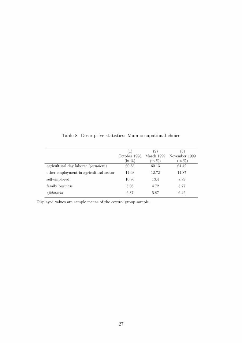
Table 8: Descriptive statistics: Main occupational choice

(1) (2) (3)October 1998 March 1999 November 1999

(in %) (in %) (in %)agricultural day laborer (jornalero) 60.35 60.13 64.42

other employment in agricultural sector 14.93 12.72 14.87

self-employed 10.86 13.4 8.89

family business 5.06 4.72 3.77

ejidatario 6.87 5.87 6.42

Displayed values are sample means of the control group sample.

27

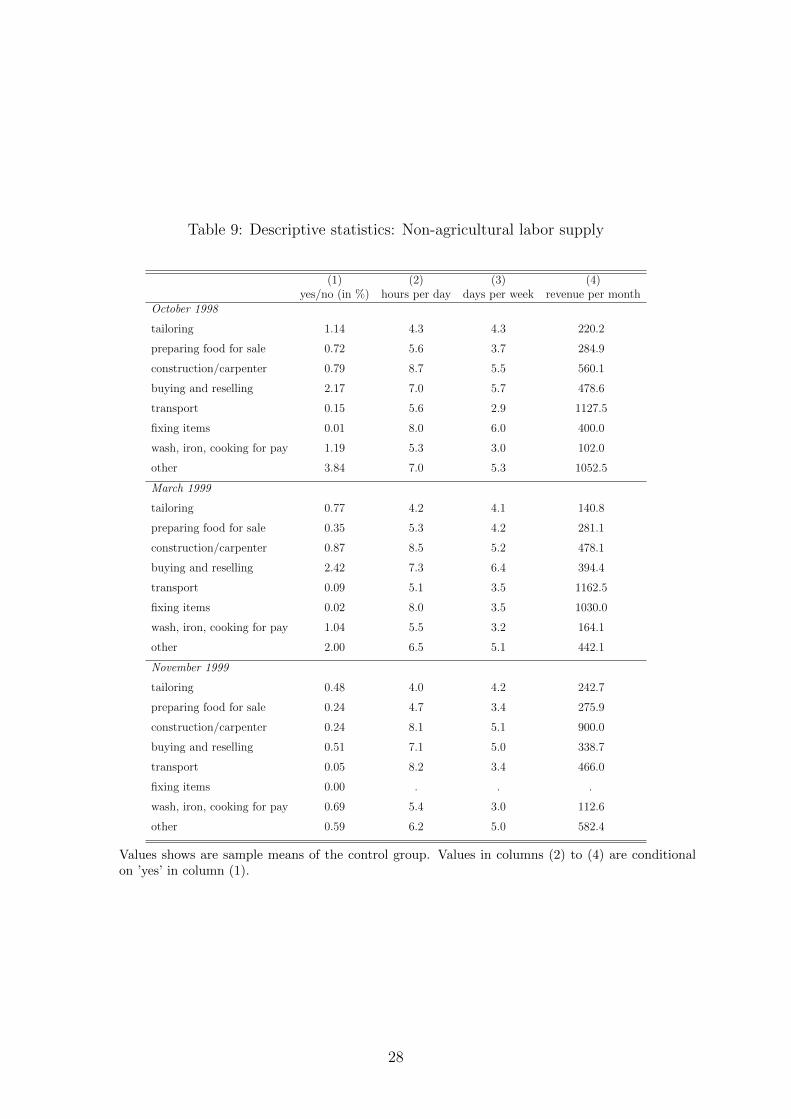
Table 9: Descriptive statistics: Non-agricultural labor supply

(1) (2) (3) (4)yes/no (in %) hours per day days per week revenue per month

October 1998

tailoring 1.14 4.3 4.3 220.2

preparing food for sale 0.72 5.6 3.7 284.9

construction/carpenter 0.79 8.7 5.5 560.1

buying and reselling 2.17 7.0 5.7 478.6

transport 0.15 5.6 2.9 1127.5

fixing items 0.01 8.0 6.0 400.0

wash, iron, cooking for pay 1.19 5.3 3.0 102.0

other 3.84 7.0 5.3 1052.5

March 1999

tailoring 0.77 4.2 4.1 140.8

preparing food for sale 0.35 5.3 4.2 281.1

construction/carpenter 0.87 8.5 5.2 478.1

buying and reselling 2.42 7.3 6.4 394.4

transport 0.09 5.1 3.5 1162.5

fixing items 0.02 8.0 3.5 1030.0

wash, iron, cooking for pay 1.04 5.5 3.2 164.1

other 2.00 6.5 5.1 442.1

November 1999

tailoring 0.48 4.0 4.2 242.7

preparing food for sale 0.24 4.7 3.4 275.9

construction/carpenter 0.24 8.1 5.1 900.0

buying and reselling 0.51 7.1 5.0 338.7

transport 0.05 8.2 3.4 466.0

fixing items 0.00 . . .

wash, iron, cooking for pay 0.69 5.4 3.0 112.6

other 0.59 6.2 5.0 582.4

Values shows are sample means of the control group. Values in columns (2) to (4) are conditionalon ’yes’ in column (1).

28

Table 10: Descriptive Statistics: Counterfactual characteristics

Eligible Households Ineligible Households

(1) (2)Mean Mean

[Std.Dev.] [Std.Dev.]Household and Community Characteristics

Gini Index for agricultural land ownership 0.71[120.7] [124.9]

Pre-program household poverty score 701.6 882.5[120.7] [124.9]

Monthly food consumption (per capita, peso value) 182.5 198.4[163.6] [153.2]

Monthly food expenditure (per capita, peso value) 137.3 169.6[130.1] [145.4]

Monthly non-purchased food consumption (per capita, peso value) 38.85 27.86[591.9] [48.1]

Monthly household disposable income (in peso) 662.1 795.3[362.6] [2129.8]

Cultivated area (in hectare) 0.46 0.75[2.77] [2.31]

Hourly wage rate 5.27 6.97[36.14] [25.12]

Livestock holding (principal component index) -0.21 0.06[2.41] [3.63]

Household size 5.44 4.82[2.60] [2.53]

Indigenous household head 0.36 0.17[0.48] [0.37]

Education of headno 32.55 26.35primary 62.03 64.52secondary 4.92 6.95tertiary 0.51 2.19

N 6857 1949

Calculations are based on the March 1999 Encel survey. Column (1) displays the sample mean ofOportunidades-eligible households residing in control villages. Column (2) displays the sample meanof Oportunidades-ineligible households residing in control villages. Standard deviations are reportedin brackets. Differences between column (1) and (2) are all statistically significant.

29