Do households use remittances to smoothconsumption?�

Dawn Teele, Atisha Kumar, Kersi Shro¤y

Yale University, May 5, 2009

Abstract

This paper explores the migration-development link by asking whether re-mittances are used to smooth consumption in rural Mexico. We constructa panel from rural household surveys collected by the Mexican governmentas part of its conditional cash transfer program, Oportunidades. The sam-ple is restricted to those households that have a migrant in any of the surveyyears (1997-2000), leaving approximately 32 thousand household-years for ouranalysis. As there is considerable variation in whether the housholds receiveremittances given migration, we estimate a sample selection logit and calculatethe inverse mills ratio for the probability that a household receives remittancesin each survey year. We then use an instrumental variables approach to es-timate the e¤ect of income shocks on remittances. To instrument for incomewe employ indices of self-reported and village aggregated shocks and lossesdue to natural disasters, as well as deviations of village-level rainfall data fromits 20 year average. Our instruments predict income with consistency, thoughthe instrumented income variable is not signi�cant in the remittance equationonce household characteristics are controlled for. The most important charac-teristics for predicting remittances include whether the migrant is spouse tothe household head, and the head of the household�s education.

�Preliminary, Please Do Not CiteyThis work has been supported by the Hewlett Foundation and the MacMillan Center at Yale

Unviersity. We would like to thank the working group on Mexican Remittances formed by GusRanis at Yale University�s Economic Growth Center for their comments at various stages of thisproject.

1

1 Introduction

The �rst decade of the twenty-�rst century has seen a tremendous movement of

ideas, people, and capital to and from the corners of the globe. Globalization, the

process of increasing market integration between big and small economies, between

strong and weak states, has the potential to fundamentally alter the distribution of

wealth and resources during our lifetimes. Some channels through which this global

redistribution has and will continue to take place are well known � development

aid, private �ows of investment capital, research institutions that fund international

scholars, and philanthropy �all recommend themselves to investment, collaboration

and redistribution with the developing world. Yet this tide of formal and institutional

�ows might not su¢ ce to lift the boats of the world�s poorest people.

Migration, the movement of one or many family members to a new location in

search of work, is one important avenue through which a household might lift its own

boat (by increasing collective resources, thereby improving welfare). This migration-

development link was �rst explored in the seminal �Surplus Labor Model�, also

known as the Lewis-Fei-Ranis model, which relates both urban and rural growth to

migration. The basic idea behind this model rests on an assumption that the rural

sector is ine¢ cient because labor is too widely available relative to need. Thus, rural

households, which are said to produce at a point where the marginal product of labor

is below the wage, could lose laborers to the industrial sector while still maintaining

the same level of output; the migrant could literally take his backpack of grain with

him as he searches for higher wages in the city (see Ranis and Fei (1961), Sen (1966)

or Lewis (1954)).

Although the Surplus Labor Model is no longer a dominant paradigm in devel-

opment economics, the insight that migration may be a key to development has

certainly persisted. Our interpretation of the relevant mechanism is not that the mi-

grant simply leaves the household, but that he or she is useful to the family because

of the transfers sent (in cash or kind) to those who were left behind. These transfers,

known as remittances, can serve the migrant�s family or community in many impor-

tant ways. Indeed, there are several narratives for why remittances matter: they

2

can facilitate village traditions by providing for ceremonies �weddings, birthdays,

baptisms and other important community events (Durand et al. 1996, 428); they can

support the construction of schools and churches (Sana 2008); allow for the private

provision of �public�goods such as access to sanitation and water (Adida and Gerod

2009); or, as we will argue in this paper, remittances can facilitate development by

increasing stability if they allow households to smooth consumption when weather,

crop losses, or natural disasters negatively a¤ect household income.

Some scholars and policy makers argue the opposite, asserting, in fact, that remit-

tances reinforce dependency in the developing world. The evidence for dependency

is mixed: Barham and Boucher (1995) �nd that that migrant-sending households

choose to participate less in the labor market, ostensibly because remittances pro-

vide enough income for the household. Further, remittances actually increase in-

equality.1 Finally, there is worry that remittances cause dependence because they

are consumed rather than invested. However, Adams (2006) �nds that rather than

bolster consumption, remittances to Guatemalan households are, in fact, invested.

When it comes to questions of the development e¤ect of remittances, di¤erent

contexts produce di¤erent results. We hope to contribute to this debate by arguing

that remittances should be considered within the context of the household (rather

than, as will be discussed in the following section, using the individual migrant) as

the unit of analysis, as their purpose is precisely to protect agricultural households

against unforeseen shocks. In using the Oportunidades data we have the advantage

of rich household characteristics and over-time variation in the migration and remit-

tance data of interest, which allows us to test whether remittances operate to smooth

consumption.

Two main methodological concerns are accounted for in our empirical strategy.

The �rst is that there is a selection mechanism which causes some migrant-sending

households to receive remittances while others do not. This concern is not purely

1It should be noted that there is still substantial disagreement concerning the proper way toanalyze inequality: Stark et al.�s (1986) method of comparing income distribution with and withoutremittances has been widely criticized for its assumption, similar to the Lewis-Fei-Ranis premise,that removing workers from the village does not negatively a¤ect output. For more on this seeKeskin�s paper at this conference, Adams (1989), Barham and Boucher (1995) etc.

3

theoretical; indeed, 34 percent of households in our sample never receive remittances

despite having migrants during at least one survey year. We correct for this selection

problem by estimating a logit regression for the probability of receiving remittances,

given a vector of household migrant characteristics (e.g. how many male migrants

are in the United States, how many female migrants are daughters of the household

head). We use the logit to calculate the inverse Mills ratio for each household year,

and then use this variable in our remittance equation.

The second methodological concern is that income and remittances are simul-

taneously realized, i.e. income may be endogenous to remittances. The Barnham

and Boucher paper cited above, which shows that there are labor market (hence

income) responses to remittances, provides some justi�cation for this worry. We deal

with endogeneity by instrumenting for income, using various self-reported shock and

loss data, as well as exogenous rainfall data, in a two-stage least squares remittance

equation.

The paper will proceed by describing in Section 2 the extant literature on migrant

motivations and the remittance response to shocks. Section 3 will set the stage

with a discussion of migration in the Mexican context, and present a highly stylized

analytical framework for remittances as a consumption-smoothing mechanism at the

household level. Section 4 contains a detailed description of our data, and Section 5

presents the results of our empirical investigation. We conclude with a discussion of

ways in which this research can be enhanced.

2 Remittances and Development

The vast majority of the literature on remittances focuses on the individual mi-

grant�s motivations to remit. Before developing a model of remittances as an income-

smoothing strategy, we turn to this literature.

2.1 Motivations for an individual migrant

Most studies that consider why migrants remit argue that the individual migrant is

the appropriate unit of analysis (Banerjee 1984; Cox 1987; Johnson and Whitelaw

1974). The research question can generally be understood as asking, �How does a

4

utility-maximizing individual take the decision to remit?� Potential answers to this

question include the following:

1. Pure Altruism: The migrant is driven by a desire to help his or her send-

ing household (i.e. the consumption of the recipient falls into the migrant�s utility

function). Studies that support this hypothesis include Bouhga-Hagbe (2006) and

Agarwal and Horowitz (2002).

2. Pure Obligation: The migrant is repaying her family for previous investment

(e.g. the cost of schooling, or of crossing the border, inculcated social mores). Hod-

dinott�s (1992) study of remittances sent to households in Kenya, Bernheim, Shleifer

and Summers (1985) and Cox (1987) are examples of work that support the �oblig-

ation�hypothesis.

3. Enlightened Self-Interest (a mixture of altruism, obligation and investment):

The migrant is driven by the altruism motive, but is also motivated by his or her

own well-being, especially in the case of anticipated returns. In a seminal paper,

Lucas and Stark (1985), explore this motivation. They argue that a model of �tem-

pered altruism or enlightened self interest�best explains remittance behavior. Using

household survey data from Botswana, they appeal to two independent variables of

interest: First, if migrants remit in order to repay prior educational investments,

households with educated migrants should receive remittances. Second, if migrants

remit as part of a household�s e¤ort to diversify risk, those households that take on

more risky production at home (e.g. by using new seeds/technology, by having cattle

as the main asset) should receive more remittances. They �nd evidence for altruism

in that the family head remits at statistically signi�cant levels, though evidence for

risk diversi�cation is mixed: households with more cattle are weakly more likely

to receive remittances. There is little evidence that the repayment of educational

investment, as proxied by migrant children of the household head, matters.

4. Insurance: To ensure a migrant�s warm welcome in case of an un-anticipated

return. Pozo and Dorantes (2006) test for the insurance motive by correlating host

economy risk variables with remittance �ows. They �nd strong evidence that those

migrants with less-developed social networks, who are undocumented, or who work

in seasonal occupations, tend to remit more. In e¤ect, migrants with uncertain

5

futures insure themselves against the need to eventually return home by remitting

more. Unlike previous literature on the subject, Pozo and Dorantes use host-country

risk variables rather than home-country household characteristics to evaluate the

insurance motive.

These studies o¤er important insights into the possible motivations of remitting

migrants; however, for development economics, the question of individual motivations

is of only secondary importance. Understanding which conditions lead to long term

human and economic development is primary, and thus what matters is whether

remittances can serve in the interest of the household. It is our contention that if

remittances allow for stability in household consumption, they can contribute to this

lasting development. We turn now to the small literature that considers household

risk and remittances.

2.2 Remittances and consumption smoothing

Agricultural households are subject to much vulnerability: price shocks for both

consumed and produced goods; malnutrition and general ill health; and threats of

natural disasters and crop blights all add to the instability of the countryside. A

number of studies have considered the role that family and community can play in

collectively protecting against these risks (see, for example, Udry 1994). A primary

concern is that with incomplete access to insurance markets, and with low or non-

existent household savings, seemingly small shocks to income may have dramatic

e¤ects on household consumption and welfare. Two recent papers �by Yang and

Choi (2007) and Quisumbing, McNevin and Godquin (2008) directly address these

issues.

Yang and Choi (2007) use micro-level data from the Philippines to analyze the

impact of income shocks on remittances. Their evidence shows that origin house-

holds use remittances as insurance. The authors use rainfall shocks as instrumental

variables for changes in income, and �nd a negative correlation between income and

remittances, meaning that remittances increase when income decreases.

Quisumbing, McNevin and Godquin (2008) also use Filipino micro data to test

whether remittances a¤ect the asset holdings, consumption expenditure, and credit

6

constraint status of households. In their analysis, the authors control for any �shocks

experienced by the origin household�and by the migrant.2

The evidence suggests that remittances positively impact expenditures on hous-

ing, consumer durables, non-land assets and total expenditures of migrant-sending

households in the Philippines. Drought shocks are found to have the biggest e¤ect

on households with below median land holdings and land size, net worth, as well as

those who have greater than median levels of schooling (Quisumbing, McNevin and

Godquin 2008, 12).

Although the two papers discussed above explore a number of important issues

regarding the impact of household shocks on remittances, they leave some critical

questions unanswered on the issue of remittances and consumption smoothing. We

believe that our study improves on the current knowledge both because we have

a dataset which o¤ers us over-time variation in household, migrant, and remittance

characteristics, but also because of the unique measures of shocks that we will employ:

shocks at the household and village level and of particular losses su¤ered by the

household. In the next section we will explore the unique characterics of our data

and sketch out a very stylized analytical framework to guide our thinking as we move

to the empirical portion of the paper.

3 Migration and Remittances in the Mexican Context

The question of whether remittances allow households to smooth consumption could

well be analyzed in a variety of settings, but is particularly salient in the case of

Mexico and the United States given the countries�historical migration linkages, and

the non-trivial contribution that remittances make to Mexican national income. The

Mexican Government estimates show that between 1990 and 2000, approximately

3.2 million migrants left Mexico for the U.S., with 77 percent making no return trip

during that period (INEGI3); further, in 2006, international remittances accounted

2The survey used in the paper includes shocks �related to agriculture, political or social events [.. .] as long as they have resulted in a loss of income or caused [the household] to become seriouslyconcerned or anxious about [their] welfare�.

3http://www.inegi.org.mx

7

for 3 percent of Mexico�s Gross National Income (Ratha and Xu, 20064).

In addition to labor �ows to the United States and other countries (including

Canada, Spain, Bolivia, Guatemala, Germany, etc.), Mexico is also witness to sub-

stantial rural-urban migration within its borders. This intra-national migration,

which we will call �internal� migration, provides an additional level on which to

understand the household remittance patterns. Between 1990 and 2000, internal mi-

grants in Mexico included 7.5 million persons, or approximately 5 percent of Mexico�s

population. Current �gures indicate that since 2000, emigration out of Mexico has

increased substantially, with 10.7 percent of persons born in Mexico residing outside

of the country (Ratha, Mahapatra, and Xu, data for 2005). However, the internal

migration �gures are only 2.7 percent of the total population (INEGI, data for 2005).

These statistics indicate that migration is a dynamic process, and present us

with many avenues for interesting research. A question that immediately suggests

itself is why has there has been a shift away from internal migration and toward

emigration out of Mexico since 2000? One answer that our research supports is that

external migration has higher returns, at least prior to the current global economic

downturn, and that households might have responded to these returns by encouraging

emigration instead of simply re-location within Mexico.

Before we turn to the data we would like to brie�y sketch an analytical framework

for understanding remittances as a consumption-smoothing strategy of households.

3.1 An Analytical Sketch

The main claim of this paper is that migration and remittances are a means to con-

sumption smoothing for migrant sending families. The basic problem for households

is to maximize per capita consumption over their lifetimes; their main decision is

where and when to send migrants.

Consider a two-stage model wherein households maximize consumption across

both stages. Total utility U for household h is a sum of the utilities from both

stages:

4http://econ.worldbank.org

8

Uh =

mXi=0

ln c1i +

mXi=0

ln c2i (1)

where c1i and c2i are consumption for household member i (where i � f1; :::;mg)

in period 1 and period 2, respectively. Summation of each of these across all migrants

is represented by C1h in the �rst stage and C2h in the second stage. In the �rst stage,

families choose whether and where to send each adult as a migrant. In the �rst

period, the family incurs a cost, x; for each migrant it sends. x can represent either

the cost of the migrant�s education or the travel fees associated with migration. This

payment is, in a sense, the premium paid by the family to guarantee remittance

transfers from the migrant.

C1h = Y1h �

nXi=0

xi (2)

Thus the household�s consumption in the �rst period, C1h; is equal to their income

in that period Y 1h , minus the costs of sending each of the n migrants. In most cases,

the higher the cost of migration xi, the higher the household expects the migrant�s

future income to be. This explains the di¤erential cost of, and future income from,

external versus internal migration.

Consumption in the second period C2h is the sum of the n migrants�consumption,

C2n, and the consumption of the m� n household members left at home C2m�n :

C2h = C2n + C

2m�n (3)

where

C2n=

nXi=0

c2i (4)

and C2m�n=m�nXi=0

c2i (5)

9

In the equations below, Y 2m�n is home country household income per capita in

the second stage, Y 2n is the income of migrant i, which is a function of the amount

spent by the family on the migration xi, and ri is the remittance amount sent by

migrant i in the second stage.

C2h = Y2m�n +

nXi=0

ri (6)

C2n =nXi=0

Y 2n �nXi=0

ri (7)

As there are diminishing returns to consumption for each household member,

the household�s utility will be maximized by a more equitable distribution in remit-

tances. We assume that migrants in the second stage earn equal to or more than

the home country average per capita earnings and thus send remittances as part of

the household�s decision to decrease income inequality and facilitate overall increase

in utility. Remittances thus must increase with declines in home country household

income per capita. We hypothesize that home country income in the second stage

is likely to be a function of shocks to the household at home, and that remittances

should show a noticeable increase following shocks that hurt household income in

the home country.

4 Household Data

The most important data for this paper come from household surveys in rural Mexico

covered by the Oportunidades conditional cash transfer program from 1997-2000.

Under the program, the national government of Mexico gives cash to households

with children under the age of 21 in both rural and semi-urban areas on the condition

that the children attend school and visit health clinics for inoculations. We draw

exclusively from the surveys conducted in rural areas.

The data begin in 1997 when the Mexican government surveyed villages in six

Mexican states � Guerrero, Hidalgo, Michoacan, Puebla, Queretaro, San Luis Potosi

and Veracruz � which were located in areas known to be extremely vulnerable. A

10

census was taken of every household and the households were subsequently given a

rating of �very poor�, �somewhat poor�, �not very poor�, �not poor�or �not poor at

all�. Of the 495 census villages in the �rst full survey, 314 were randomly selected to

receive a Oportunidades transfer during the �rst two years of the program (summer

1998-summer 2000). The remaining 181 villages were used as a control and received

the transfer after 2000. In the treated villages, households that were �somewhat

poor�or �very poor�should have received an Oportunidades transfer, but the data

represents a random sample of the households in each of the treatment and control

villages. Over the course of three phases, the bene�ciaries are spread among the 32

Mexican states, but the data for the latter phases was released only recently so our

sample will only cover the preliminary program from 1997-2000.5 A map showing

the location of our sample can be found in Appendix C.

One important fact to keep in mind when considering our results is that the

villages in our sample were chosen from a pool of very poor villages and are ar-

guably not representative of Mexico as a whole. This limits the generalizability of

our results, but nevertheless allows us to draw meaningful conclusions for an impor-

tant demographic.6 The data is also limited because in 1997, the census year, each

household could only respond to questions about �ve migrants, but in later years the

respondent was allowed to answer for as many migrants as the household would like

to report. Less than one percent of the households have more than �ve migrants,

however, so this omission should have negligible e¤ects on our results.

5Oportunidades was structured by the Mexican government to reach the �the poorest (or mostmarginal) rural localities�(Coady 1) and thus targets the �worst o¤�people in these already-poorregions in Mexico. The program �aims to improve living standards of poor families�by targetingthree components of development: education, health and nutrition (Behrman and Todd 1).

6One substantive bene�t of using the Oportunidades data as opposed to the INEGI samplesurvey, the Mexican Migration Project, or the Mexican Family Life Survey, is the speci�city ofremittance amounts and migrant location information. Indeed, the INEGI does not distinguishbetween remittance payments made to the household from migrants and those that come fromfamily or non-family members who reside in the same village. If the migrant is internal, the surveyrecords in which state he or she resides; unfortunately, we have no way of knowing in what countryan �extranjero�or external migrant is located but we are con�dent that most are in the U.S.

11

4.1 Migration and Remittance Data

The Oportunidades survey questions respondents about migration and remittances

in the October/November enumeration during each of the survey years. A repre-

sentative member of each household (almost always the household head) is asked

whether someone has left the household and not returned during the last �ve years.

In the full dataset, 34 percent of households report ever having a migrant. Restrict-

ing our sample to this group leaves us with data covering 31,753 household years.

Appendix A contains a table of summary statistics by survey year.

As can be seen in Appendix A, there is considerable variation in the percent

of households that have migrants in each year, ranging from 10 percent in 1997

to 50 percent in 1999 and then dips low again. The number of migrants also varies

considerable over the sample. Appendix D presents histograms by year of the number

of migrants in each household. Finally, from the sample of households that have

migrants in a given year, there is considerable variation in those that also receive

remittances, with 60 percent of 1997 migrant households receiving remittances, down

to 33 percent in 1998 and 23 percent in 2000.

Given that a household has migrants, the enumerator then asks �has this mi-

grant sent any money home? What is the amount?� In 1997 the time referent for

this question was 12 months, though in later years the household was asked about

remittances during the last 6 months. Thus, to make the data compatible, we have

multiplied the remittance amounts for 1998-2000 by 2.

The two dependent variables we will analyze concern whether a household receives

remittances and the amount received. First, for each household i in village v during

year t, the household either receives remittances or it does not, hence:

rivt � f0; 1g (8)

We will construct a vector that represents a household-migrant pro�leMivt, which

includes, for each household in the sample, the number of adult male and female

migrants, the number of each who are living outside of Mexico, and the number

that are sons and daughters of the household head (to signify closeness of kin). This

12

household-migrant pro�le will be used to estimate the probability that the household

receives remittances.

Second, we will estimate a �remittance equation�using the remittances received

Rivt, where R is the total remittance received by the household i in village v during

year t as the dependent variable.7 The following will be included as explanatory

variables in the remittance equation: the migrant�s gender, location (in one of Mex-

ico�s states or abroad), and the relationship to the household head. These variables

are described in Appendix A, and a bar graph showing the kinship of migrants is

included in Appendix D. Interestingly, only 2.5 percent of migrants are spouses to

the household head, whereas 74 percent are children of the head, and 8 percent are

their grandchildren.

The remittance equation also contains a vector of basic household characteristics

Hivt , which includes whether a household owns the land their house is on, whether

they own other agricultural land, and the size of the household�s herd (cows and

cattle) that the family own in a given year. The importance of the ownership and

herd variables were delineated by Lucas and Stark (1985) as both a risky asset and

something that could be inherited. Because we think that there is a relationship be-

tween these variables and one�s potential to inherit in the future, we have interacted

all of the Hivt with the number of sons in a household to unpack the inheritance hy-

pothesis. A complete list of variables and their de�nitions are available in Appendix

A.

4.2 Shock Data

To circumvent issues of simultaneity with the remittance and income vectors, we use

a variety of data on agricultural shocks to instrument for income. For variables that

come from the Oportunidades dataset, we use the shock data from the same survey

in which the migration and remittances questions are asked, and aggregate up to the

annual level.7Note that all monetary values are recorded in real 1997 pesos, and that there are approximately

ten pesos to the dollar throughout our sample frame. Summary statistics of the dependent variablescan be found in Appendix A.

13

� Self-reported experience of natural disaster (1998-2000): The raw data are

binomial variables that indicate whether a household has su¤ered from drought,

�ood, frost, �re, blight, earthquake or hurricane in the past 6 months:

sivt = f0; 1g with s � fflood; drought; :::; etc:g (9)

For each household i in village v during year t: Bar graphs showing both the

breakdown of whether a shock occurred, and which disasters were most prevalent,

by state, can be found in Appendix F.

� Self-reported loss data (1998-2000): similar to the natural disaster data, thehousehold was asked what the consequences of the disasters were. We have

binomial indicators for whether they lost land for crop cultivation, lost crops,

the house, various household items, or whether an animal or member of the

household was injured or died.

� Village level shock indices (1998-2000): because households might make riskierinvestments in the face of remittances (which might cause the shocks or losses

su¤ered to be higher in these households), we constructed shock indices for

each of these variables at the village level. The indices are the sum of the

household shocks sivt for each village, divided by the number of households in

that village during the survey year, nivt:

Ss;vt =500Pn=2

sivtnivt

(10)

Given this formulation, Ss;vt is a continuous variable that goes from zero to one.

We have constructed histograms and bar charts to demonstrate the distribution of

these shock variables, available in Appendix F.

� Deviation of rainfall from its 20 year average (1997-2000): Since Oportunidadesdoes not ask the shock and losses questions in the �rst year, and to counter

the possibility of bias due to the self-reporting, we also used rainfall data from

14

the Climate Research Unit�s Central America database (Mitchell and Jones,

2005). Using monthly rainfall data from 1981-2000, we constructed a 20 year

average precipitation variable, p20w, indexed to the rain grid at point w, and

then constructed yearly averages for our survey years t: p1wt. Thus Pwt is point

w�s deviation from the 20 year average preciptiation in year t

Pwt = p1wt � p20w (11)

We matched the grid points to the villages in our sample by using the Hawths

Analysis tools in ArcGIS. In the empirical portion we will look both at Pwt for the

grid point that is closest to the village, and at the same measure weighted by its

inverse distance ( 1dwv)Pwt which gives the data more emphasis when the gridpoint is

closer to the village.8

5 Empirical Analysis and Results

5.1 Strategy

In the theoretical portion of this paper we argued that migration is a strategy that

households use to smooth consumption in the face of economic uncertainty. This

uncertainty is borne out in each year by reductions to household income that cause

family-oriented migrants to remit more than they would in the absence of such re-

ductions.

Our empirical strategy will involve three steps. First, we estimate a log-odds

(logit) regression for the decision to remit:

rivt = �0 + �xMivt + Tiv + uivt (12)

Where Mivt represents a vector of characteristics relevant to a household�s mi-

gration characteristics, Tiv is a dummy that is equal to one if the household resides

8The inverse distance weighted average has been informed by Sheppard�s (1968) discussion. Wewould like to take a weighted average of precipitation for the n closest rainstations, but for thisiteration of the paper we have been unable to resolve the problem of directional repetition.

15

in an Oportunidades �treatment�village and was classi�ed as eligible to receive the

cash transfer, and uivt is the household year�s error term.

Second we calculate the inverse Mills ratio for each observation and use this new

variable �the mills ratio �as a regressor in the remittance regression. Use of the

Mills ratio, also known as the selection hazard or �Heckman�s�lambda, was proposed

by Heckman (1979) to correct for processes of self selection by the individuals being

analyzed In our analysis, the self-selection we are concerned with has to do with

whether a household receives remittances in a given year.9 The inverse Mills ratio,

�ivt; is given by the following equation:

�ivt =�(rivt)

1� �(rivt)(13)

where � is the density function, � is the cumulative distribution function for

a standard normal variable, and rivt is the predicted value obtained by the logit

regression in the �rst step for each household i in village v during year t. The inverse

Mills ratio is a monotonically decreasing function of the probability of being in the

sample of households with remittances on any given year. Thus as E(rivt) ! 1;

given the explanatory variables contained inM and T , �ivt decreases. In the second

step, then, a lower value for �ivt corrects for the high probability of inclusion in the

sample. 10

Third, we estimate the remittance function using a two-stage least squares regres-

9In essence, the population that we consider in our analysis �those households who had migrantsduring at least one of the Oportunidades survey years �is not a random draw of the population.Thus, whether a given household has remittances (and the amount of these remittances) is alsonon-random. As Heckman elegantly describes the problem, ��tted regression functions confoundbehavioral parameters of interest with parameters of the function determining the probability ofentrance into the sample,�when self-selection occurs without correction, (1979:154).10The inverse Mills ratio also helps to take account of the indirect e¤ects of variables that appear

in both stages of the regression, so long as at least one variable appears only in the �rst stage. Theregressor that will be left out as we move to the next estimates will be Tv, the dummy that controlsfor whether a household was eligible to receive the Oportunidades transfer. The rationale behindexcluding this particular variable is that though being eligible for a transfer may a¤ect whether ahouseholds receive remittances (e.g. an eligible household may be too poor to have migrants), itshould not a¤ect the amount of remittances in any way that isn�t already captured in the incomevariables.

16

sion (2SLS) where the dependent variable, remittance per migrant Rivt is dependent

on a vector of household characteristics Hivt, the income of the household Yivt, the

inverse Mills selection variable �ivt, and a household speci�c error term.

Rivt = �0 + �xHivt + �pYivt+�ivt + uivt (14)

We instrument for household income Yivt using various indicators of shock and

loss S.

Yivt=�0 + �S+ v (15)

S=(Svt;Sivt; :::; Pvt; Panivt ) (16)

The S and v components will have errors depending on whether the shock vari-

ables are aggregated to the household or the village level. P anivt is the interaction

between the precipitation variable and the number of small animals in the house-

hold, which allows the precipitation indicators to vary by household.11

Our assumption in using the instrumental variables is that the shock variables

have an e¤ect on remittances only through their e¤ect on income, meaning that v is

orthogonal (strictly uncorrelated) with uivt. We believe that shocks will operate in

the following way: if the shock a¤ects income, the migrant will be inclined to remit

payments; if not, the remittance cannot be attributed to consumption smoothing.12

11The number of small animals in the household has approximately zero correlation (r=-0.0035,p-val=0.53) to remittances per migrant12We believe this to be a valid assumption, though perhaps a simple vignette might help to

illustrate the point: suppose that a mother�s relationship with her daughter is such that the motherhas agreed to help the daughter smooth her consumption during her college years. One day thedaughter is robbed on the street, her purse is stolen and along with it a cell phone and some hundreddollars or so of cash. This is a situation in which the daughter has su¤ferd from a shock that hashad an impact on her ability to consume (both because the money was taken and because she willhave to replace the cell phone). The mother, acting in her role as consumption smoother, is quickto the rescue: a check is in the mail the next day. Now suppose that instead of being robbed witha fully equipped pocketbook, the daughter was instead accosted on her way to the grocery store,with nothing but an empty canvas bag (and a credit card safely tucked in her pocket). In this case,the mother has no obligation to send any money for consumption smoothing as the shock hasn�t

17

5.2 Results

5.2.1 Logit estimation to calculate inverse Mills Ratio

Table 3 shows the results from the �rst stage of our regression, both models are run

using the logit speci�cation, and marginal e¤ects are the reported coe¢ cients. The

�rst model looks at the probability that a household will have remittances using

broadly aggregated categories of migrant characteristics. The �rst �ve variables in

column (1) are dummy variables equal to one if the household has, respectively,

female or male migrants, a migrant residing outside of Mexico, or migrants that are

either the son or daughter of the household head. The signs of the coe¢ cients on each

of these variables �t nicely with our intuition about which types of migrants remit.

For example, the most important economic determinant of remittances is whether

the migrant resides outside the United States, with both male migrants and sons of

the household heads also having positive e¤ects on the probability of remittances.

The coe¢ cient for female migrants is negative and statistically signi�cant, though

daughters are more likely to remit. Finally, the treatment dummy, which equals one

if a household is in a treated village and eligible for the transfer, has a negative e¤ect

on the marginal propensity of a household to receive remittances.

Column (2) in Table 3 disaggregates the dummy variables from the �rst column

to indicate their cardinal values, i.e. we include the numbers of migrants that each

household has in a given year that falls into each category. The direction of the

coe¢ cients in column (2) mimic those in the former column, though the treated and

son migrant variables no longer maintain their signi�cance. We read these coe¢ cients

as saying that the marginal e¤ect of having an additional son migrant is zero, though

of course the marginal e¤ect of having son migrants, in general, is non-trivial.

Following Wooldridge (2005), we calculated a goodness of �t measure to estimate

the percent correctly predicted by each of our models. The equation is as follows:

if

G(�0 + �xMivt + Tiv) > :5

then the model predicts a probability of 1;

a¤ected the daughter�s ability to consume.

18

if

G(�0 + �xMivt + Tiv) � :5

then the model predicts a probability of 0.

Using this formulation, column (1) gets the correct prediction in 76.4 percent

of the cases, whereas column (2) gets the correct prediction in 89.9 percent of the

cases. Because of its superior prediction power, and the fact that we retain more

observations, we will use the model in column (2) to predict the inverse Mills ratio,

�ivt:

5.2.2 Do our instruments do a good job predicting income?

Before we proceed with the instrumental variables approach outlined above, we turn

to Tables 4 and 5 to see whether our self-reported shock variables or rainfall variables

(respectively) do a good job of predicting income.

For each type of shock: village shock index, household shock dummies, and house-

hold loss index, Table 4 contains the results of regressions run on log of household

income for both random e¤ects and �xed e¤ects speci�cations. For the village shock

index, the �xed e¤ect will be at the village level, for the household variables, the

�xed e¤ect is at the household level.

Columns (1) and (2) of Table 4 show that, though all indices except for the frost

index have a negative e¤ect on income, those that are statistically signi�cant in both

models include only the blight and hurricane indices. We expect the standard errors

in these two speci�cations to be quite large, given the fact that the index is on the

village level, but the log of household income is measured per household-year.

Columns (3) and (4) of Table 4 contain household dummies for the various shocks.

These variables indicate that there is a negative relationship with income for all but

the drought variable under the random e¤ects estimate. The �xed e¤ect model

shows that drought, frost, earthquake and hurricane all have statistically signi�cant

and negative relationships with income. This model is likely closer to the true model

as it allows for heterogeneity between households (i.e. it allows for each household

to have a unique intercept).

19

Finally, columns (5) and (6) show the relationship between log household income

and self-reported loss dummies. These results are interesting: though losing crops

has a negative and statistically signi�cant relationship with income, losing animals is

signi�cant and positive. It would be a stretch to surmise what is causing the positive

relationship between income and lost animals, and we will not attempt to do so at

this time.

Table 5 turns to our exogenous instruments to see whether rainfall shocks are

good predictors of income. Column 1 considers the e¤ect on income of rainfall from

the closest station. The variables include the deviation from the 20 year mean, and

that deviation squared. Column (1) includes village �xed e¤ects, as each household

in the village will have the same data point, and no signi�cant results appear. The

second regression looks also at the closest rain station, but this time the deviation

and deviation squared have been multiplied by a scalar, the number of small animals

in the household, to allow the data to vary at the household level. The number

of small animals in the household has approximately zero correlation (r=-0.0035,

p-val=0.53) to remittances per migrant (the dependent variable in the next step).

Column (2) shows an inverted U relationship between deviation from 20 year rainfall

and income: Income increases but at a decreasing rate when rainfall is higher than

average.

Column (3) shows the deviation from 20 year weighted average (and its square)

for the �ve closest rainfall stations. The relationship exhibited at the village level is

that of a U, but when we allow the vectors to vary by household, using the number

of small animals, the relationship discerned in column (2) remains. The coe¢ cients

and standard errors in all of these columns are quite small, indicating that, though

they might be statistically signi�cant, the economic signi�cance might not be as

important when other variables are controlled for.

5.2.3 Is income, instrumented by shocks, driving remittances?

Tables 6, 7 and 8 present the instrumental variable remittance equations in the

following order: Table 6 looks at self-reported shocks, losses, and village indices.

Table 7 looks at deviations from 20 year average rainfall at the closest rainstation, and

20

Table 8 looks at deviations of weighted 20 year averages for the 5 closest rainstations.

The dependent variable follows our analytical sketch and represents the remittance

per migrant. When the household had no migrant, the dependent variable takes on

the value of zero.

Each regression includes the variable imr which is the inverse Mills ratio that was

calculated for each household year using the second column of coe¢ cients in Table

3. In all three tables, the inverse Mills variable is the largest and most important

predictor of receiving remittances. If the IMR is high, the remittances that the

households receive are lower. This is as expected as the inverse Mills ratio �punishes�

those households that were more likely to receive remittances based on the migrant

characteristics in Table 3.13

It is interesting to note that income (as instrumented by the shock variable speci-

�ed in the column header of each table) is never a statistically signi�cant determinant

of remittances once other variables are controlled for. In Table 6, income has the

expected negative sign: if income increases, remittances should decrease (in fact, if

the household is operating as a unit with the migrant, higher income should mean

negative remittances, something that is not observed in the data).14 Tables 7 and

8 show no signi�cant relationship between income and remittances, and the sign

bounces around to a great extent.

Aside from the inverse Mills ratio, the second best predictor of remittances is

whether the migrant was the spouse of the household head, which occurs in only

1.67 percent of our cases. Our analytical framework speci�ed that the household

smooths consumption by deciding where and when to send a migrant, and that it

receives more remittances when times are tough. The assumption that we made is

that the migrant remains a member of the household though he or she lives elsewhere,

and it is for this reason that he or she acquiesces to the bargain. The positive and

13In essence, the characteristics that were likely to cause selection into the remittance pool shouldnot count again, positively, towards those determinants of the remittance function.14Our de�nition of income can be negative, however, if transfers out of the house were greater

than income plus transfers in. Unfortunately there is no way to link up transfers out of the housewith transfers to migrants, however the survey does ask whether each transfer was for someone �inthe same village��in a close village�or �far away�, and for the majority of those cases (76-88 percent)were not to persons located far away.

21

signi�cant coe¢ cient on the spouse variable across all speci�cations may imply that

those members who see themselves as remaining in the family are indeed more likely

to remit. We plan to, in the next iteration, look at the single cross section of 1998 in

which there are better measures of the reason for leaving. We think that daughters

who leave to get married will join a new household and be less likely to remit, all

else equal.

The �nal explanatory variable of note is that the head of the household�s educa-

tion, in all speci�cations but one, is positively related to remittances per migrant.

It could be that this variable is indicative of the migrant�s education, which, when

higher, would allow for higher labor market returns.

6 Conclusions and Future Research

The end of this paper seems, in fact, to suggest the beginning of a larger research

project. We have shown that though shock variables � self reported, aggregated

indices, and exogenous rainfall data �seem to predict income with some consistency,

income, when instrumented by these shocks, is not a great predictor of remittances.

This means that we must either re-think our model (i.e. argue for other explanations

of migrant remittances) or we must be more particular with the de�nition of the

migrant: Is a daughter who marries into another household, strictly speaking, a

migrant? Is a student that leaves for school, strictly speaking, a migrant? Should

we expect di¤erent remitting patterns based on whether the individual is likely to

return to the household (e.g. the spouse), or based on their immigration status (e.g.

documented or undocumented)? These and other important questions are certainly

worth considering in future research.

22

References

[1] Adams, R.H. 2006 Journal of African Economies 2006 15(Supplement 2):396-425

[2] Adida, Claire L., and Desha M. Girod (2009). Do migrants improve their home-

towns? Remittances and Access to Public Services in Mexico, 1995-2000. Com-

parative Political Studies (forthcoming).

[3] Agarwal R, Horowitz AW (2002) �Are international remittances altruism or

insurance? Evidence from Guyana using multiple-migrant households�. World

Dev 30(11):2033�2044

[4] Amuedo-Dorantes, Catalina, Bansak, Cynthia, and Susan Pozo (2005). On the

remitting patterns of immigrants: evidence fromMexican survey data. Economic

Review 1: 37-59

[5] Amuedo-Dorantes Catalina, and Susan Pozo (2006). �Remittances as insurance:

evidence from Mexican immigrants.�Journal of Population Economics, Journal

of Population Economics, 19(2).

[6] Arenas E. (2007), �Health Selection of Internal migration in Mexico: evidence

from the Mexican family life survey�, University of California Los Angeles.

[7] Banerjee, B. 1984. �THE PROBABILITY, SIZE, AND USES OF REMIT-

TANCES FROM URBAN TO RURAL-AREAS IN INDIA.� Journal of De-

velopment Economics, 16:3, pp. 293-311.

[8] Barham, Bradford & Stephen Boucher. 1995. Migration, remittances, and in-

equality: estimating the net e¤ects of migration on income distribution. Journal

of Development Economics, (55) p.307-331.

[9] Bernheim, BD, Shleifer, A, Summers, LH (1985) �The Strategic Bequest Mo-

tive.�The Journal of Political Economy 93(6); 1045-1076

[10] Bougha-Hagbe J. (2006). Altruism and workers? remittance: evidence from

selected countries in the Middle East and Central Asia, IMF working paper.

[11] Coady, David P. �An Evaluation of the Distributional Power of PROGRESA�s

Cash Transfers in Mexico�. Discussion Paper 117, Food Consumption and Nu-

trition Division of the International Food Policy Research Institute

[12] Cox, D. (1987), Motive for Private Income Transfers, Journal of Political Econ-

23

omy, 95, pp.508-46

[13] Creighton M. (2008), �Moving up or moving on: the role of parental aspirations

to migrate in their children�s education in Mexico�, University of Pennsylvania.

[14] De la Brière B, Sadoulet E, de Janvry A, Lambert S (2002) �The roles of desti-

nation, gender, and household composition in explaining remittances an analysis

for the Dominican Sierra�Journal of Dev Econ 68(2):309�328

[15] Durand, J., E. A. Parrado, and D. S. Massey. (1996). Migradollars and Devel-

opment: A

[16] Reconsideration of the Mexican Case. International Migration Review, 30(2),

423-44.

[17] Heckman, J. (1979), Sample Selection Bias as a Speci�cation Error, Economet-

rica, 47, pp.153-161

[18] Hoddinott, John (1992) �Modelling Remittance Flows in Kenya.�J Afr Econ

1(2):206�232

[19] Johnson, G. E. and W. E. Whitelaw. 1974. �URBAN-RURAL INCOME

TRANSFERS IN KENYA - ESTIMATED-REMITTANCES FUNCTION.�

Economic Development and Cultural Change, 22:3, pp. 473-79.

[20] Lewis, W.A. (1954). �Economic development with unlimited supplies of labor,�

The Manchester School of Economic and Social studies (22): 139-191. Reprinted

in A.N. Agarwala and S.P. Singh, eds., The Economics of Underdevelopment.

Bombay: Oxford University Press, 1958.

[21] López-Córdova E.(2005), Globalization, Migration, and Development: The Role

of Mexican Migrant Remittances, Economia, 6(1), pp.217-256.

[22] Lucas, Robert E.B., Stark, O. (1985) �Motivations to Remit: Evidence from

Botswana�Journal of Political Economy 93(5)

[23] Massey, D. S. and K. E. Espinosa. 1997. �What�s driving Mexico-US migration?

A theoretical, empirical, and policy analysis.�American Journal of Sociology,

102:4, pp. 939-99.

[24] Mitchell, Timothy D., Jones, Philip D. (2005). �An Improved Method of Con-

structing a Database of Monthly Climate Observations and Associated High-

Resolution Grids.� INTERNATIONAL JOURNAL OF CLIMATOLOGY 25,

24

693?712

[25] Paxson, C. 1992. �Using Weather Variability to Estimate the Response of Sav-

ings to Transitory Income in Thailand.�American Economic Review. 82/1.

[26] Quisumbing , Agnes R., S. McNiven, M. Godquin. (2008). Shocks, Groups, and

Networks in Bukidnon, Philippines. CAPRiWorking Paper No. 84, International

Food Policy Research Institute (IFPRI).

[27] Ranis, G., and J. Fei (1961). �A theory of economic development,�American

Economic Review, (5): 533-565.

[28] Sana M, Massey DS (2000) Seeking social security: an alternative motivation

for Mexico�U.S. Migration. Int Migr 38 (5):3�23

[29] Sen, A.K. (1966). �Peasants and dualism with or without surplus labor,�Journal

of Political Economy 77: 425-450.

[30] Silver, A. (2006), �Families across borders: The e¤ects of migration on family

members remaining at home�, Presentado en Population Association of America

2006.

25

A Summary Statistics

Table 1: Descriptive Statistics of Households with Migrants

Variable Names 1997 1998 1999 2000 All

has migrant in survey year 0.10 0.47 0.49 0.40 0.37

(0.30) (0.50) (0.50) (0.49) (0.48)

=1 hh ever has remit 0.34 0.35 0.34 0.34 0.34

(0.48) (0.48) (0.48) (0.47) (0.48)

Internal Remittances 28.35 811.99 468.49 143.07 367.16

(354.00) (12012.90) (7812.32) (2744.39) (7370.15)

External Remittances 260.13 321.97 389.45 628.96 396.29

(3250.34) (4418.57) (5024.92) (7038.87) (5084.25)

total remittances 288.48 1133.97 857.94 772.04 763.45

(3274.03) 1(2781.14) (9270.74) (7548.77) (8940.30)

Remittances Per Migrant 214.46 785.43 609.09 568.84 544.35

(2195.02) (8966.19) (6773.53) (5774.92) (6431.93)

=1 hh has external migrant 0.52 0.16 0.15 0.23 0.20

(0.50) (0.37) (0.36) (0.42) (0.40)

=1 hh has male migrant 0.77 0.61 0.60 0.67 0.63

(0.42) (0.49) (0.49) (0.47) (0.48)

=1 hhhas female migrant 0.35 0.52 0.58 0.60 0.55

(0.48) (0.50) (0.49) (0.49) (0.50)

=1 hh has migrant daughter 0.31 0.49 0.49 0.46 0.47

(0.46) (0.50) (0.50) (0.50) (0.50)

=1 hh has migrant son 0.63 0.56 0.52 0.54 0.54

(0.48) (0.50) (0.50) (0.50) (0.50)

number adult female mig 0.04 0.34 0.37 0.32 0.27

(0.25) (0.70) (0.68) (0.66) (0.62)

number of adult male mig 0.10 0.39 0.39 0.37 0.31

(0.39) (0.73) (0.71) (0.71) (0.66)

number female external 0.01 0.03 0.03 0.03 0.03

Continued on next page...

26

... table 1 continued

Variable Names 1997 1998 1999 2000 All

(0.13) (0.21) (0.20) (0.22) (0.19)

number adult external 0.06 0.09 0.08 0.11 0.09

(0.31) (0.38) (0.35) (0.39) (0.36)

number of son migrants 0.08 0.37 0.34 0.30 0.28

(0.37) (0.75) (0.70) (0.66) (0.65)

number of daughter mig 0.04 0.33 0.32 0.24 0.23

(0.24) (0.72) (0.66) (0.57) (0.59)

=1 if hh in a treatment village 0.62 0.62 0.60 0.61 0.61

(0.49) (0.49) (0.49) (0.49) (0.49)

=1 if hh receives progresa 0.29 0.30 0.45 0.46 0.37

(0.45) (0.46) (0.50) (0.50) (0.48)

Sum of Cows and Cattle 1.35 0.17 0.91 0.94 0.83

(4.11) (1.18) (3.15) (4.20) (3.39)

son migrant x herd 1.45 0.09 0.44 0.68 0.46

(4.79) (0.87) (1.79) (2.98) (2.32)

=1 if hh owns land house 0.93 0.93 0.93 0.93 0.93

(0.26) (0.26) (0.26) (0.25) (0.26)

son migrant x own house land 0.60 0.52 0.49 0.50 0.51

(0.49) (0.50) (0.50) (0.50) (0.50)

=1 if hh owns land for ag, other 0.70 0.71 0.71 0.71 0.71

(0.46) (0.46) (0.45) (0.45) (0.45)

son migrant x agric land 0.47 0.39 0.38 0.39 0.39

(0.50) (0.49) (0.49) (0.49) (0.49)

village drought index . 0.36 0.47 0.13 0.32

( .) (0.27) (0.29) (0.19) (0.29)

village �ood index . 0.04 0.08 0.02 0.04

( .) (0.07) (0.15) (0.03) (0.10)

village frost index . 0.04 0.16 0.03 0.07

( .) (0.06) (0.24) (0.08) (0.16)

village �re index . 0.01 0.00 0.00 0.01

Continued on next page...

27

... table 1 continued

Variable Names 1997 1998 1999 2000 All

( .) (0.04) (0.02) (0.00) (0.03)

village blight index . 0.10 0.05 0.01 0.06

( .) (0.16) (0.08) (0.03) (0.11)

village earthquake index . 0.00 0.07 0.00 0.02

( .) (0.01) (0.19) (0.02) (0.11)

village hurricane index . 0.01 0.06 0.00 0.03

( .) (0.04) (0.12) (0.02) (0.08)

=1 hh drought . 0.39 0.48 0.14 0.34

( .) (0.49) (0.50) (0.35) (0.47)

=1 hh �ood . 0.04 0.09 0.02 0.05

( .) (0.20) (0.29) (0.12) (0.22)

=1 hh frost . 0.04 0.17 0.03 0.08

( .) (0.20) (0.38) (0.18) (0.27)

=1 hh �re . 0.01 0.00 0.00 0.01

( .) (0.11) (0.07) (0.04) (0.08)

=1 hh blight . 0.12 0.06 0.01 0.06

( .) (0.32) (0.23) (0.10) (0.24)

=1 hh earthquake . 0.00 0.07 0.00 0.02

( .) (0.04) (0.25) (0.04) (0.15)

=1 hh hurricane . 0.01 0.07 0.00 0.03

( .) (0.11) (0.25) (0.06) (0.16)

=1 lost land . 0.06 0.22 0.04 0.11

( .) (0.24) (0.42) (0.19) (0.31)

=1 lost crop . 0.38 0.50 0.14 0.34

( .) (0.48) (0.50) (0.35) (0.47)

=1 lost house . 0.01 0.01 0.00 0.01

( .) (0.09) (0.11) (0.05) (0.09)

=1 lost goods . 0.00 0.01 0.00 0.00

( .) (0.04) (0.09) (0.04) (0.06)

=1 death in fam . 0.00 0.00 0.00 0.00

Continued on next page...

28

... table 1 continued

Variable Names 1997 1998 1999 2000 All

( .) (0.02) (0.02) (0.00) (0.02)

=1 lost animals . 0.04 0.06 0.01 0.03

( .) (0.20) (0.23) (0.09) (0.18)

=1 hh member injured . 0.00 0.00 0.00 0.00

( .) (0.03) (0.04) (0.02) (0.03)

average rainfall, closest 959.03 1030.80 1109.97 1248.22 1084.04

(450.62) (522.69) (523.82) (569.03) (528.21)

20-year av rainfall, closest 1002.44 1001.66 1005.02 1005.49 1003.61

(463.24) (461.81) (463.17) (458.69) (461.75)

deviation from 20 yr av -43.41 29.14 104.94 242.74 80.44

(43.76) (99.09) (72.27) (126.54) (138.54)

inverse dist closest station 7.18 7.19 7.16 7.17 7.18

(7.96) (8.06) (7.98) (7.98) (8.00)

distance to rain station 1 0.31 0.31 0.32 0.33 0.32

(2.69) (2.67) (2.82) (2.86) (2.76)

deviation from 20 year weig av 26.96 60.53 86.73 142.73 78.09

(52.64) (78.08) (70.31) (90.65) (85.06)

29

B Di¤erences in Means Tables

Table 2: Di¤erence in Means Tests: Compare migrant HHs by whether they everreceived remittances

Obs Mean Obs Mean Di¤erence P-Valuenumber people in hh 22873 5.54 2383 4.68 0.86 0.00number of kids in hh <15 27865 2.29 3251 2.07 0.22 0.00number of families in hh 27616 1.02 3158 1.02 0.00 0.74Number of migrants 28429 0.55 3324 1.88 1.33 0.00number rooms in hh 27616 2.20 3158 2.30 0.10 0.22total yearly hh income 28429 38946.10 3324 31922.50 7023.60 0.61head of hh education 27616 2.17 3158 2.08 0.08 0.06=1 if male is head of hh 27602 0.88 3156 0.83 0.05 0.00head of hh speaks spanish 27616 0.27 3158 0.20 0.07 0.00House has plumbing 27533 0.08 3150 0.08 0.01 0.29House has electricity 27596 0.77 3154 0.81 0.04 0.00=1 if hh owns house 27616 0.97 3158 0.97 0.00 0.40=1 if hh owns land house is on 27616 0.93 3158 0.94 0.01 0.02=1 hh owns land for ag 27616 0.71 3158 0.70 0.01 0.47Number of Cattle 28418 0.39 3324 0.36 0.03 0.47=1 if own 1 car, =2 if more 27616 0.12 3158 0.14 0.02 0.00average ed of adults in hh 27605 3.70 3157 3.64 0.05 0.20average ed of adult males 26265 3.86 2898 3.85 0.01 0.89average ed of adult females? 27087 3.26 3107 3.20 0.06 0.21percent of resp who are literate 27616 0.67 3158 0.68 0.01 0.01percent of resp speak Spanish 27616 0.21 3158 0.16 0.05 0.00

30

C Map of Sample

Mexico: Villages in Progresa Sample

Sonora

Chihuahua

Durango

Oaxaca

Jalisco

Chiapas

Sinaloa

Zacatecas

Coahuila De Zaragoza

Tamaulipas

Guerrero

Nuevo Leon

Puebla

Veracruz­Llave

Yucatan

Campeche

San Luis Potosi

Baja California Sur

Nayarit

Quintana Roo

Tabasco

Mexico

Hidalgo

Guanajuato

Baja California Norte

Michoacan de OcampoColimaMorelos

Queretaro de Arteaga

Tlaxcala

Aguascalientes

Distrito Federal

Legend

control n=3,119

treatment n=4,985

31

D Histograms of Summary Statistics

050

100

050

100

0 5 10 0 5 10

1997 1998

1999 2000

Perc

ent

Number of migrantsObservations:31753

Migrants per family, by year

010

2030

010

2030

0 20000 40000 60000 0 20000 40000 60000

1997 1998

1999 2000

Perc

ent

Per capita income (Outliers>60000 removed)values in real 1997 pesos; non­remittance income

n = 31594Per Capita Income, by year

32

E Histograms of Remittance Data

010

2030

40Pe

rcen

t

0 5000 10000 15000 20000Internal Remittances

05

1015

Perc

ent

0 5000 10000 15000 20000External Remittances

05

1015

20Pe

rcen

t

0 5000 10000 15000 20000total remittances

010

2030

40Pe

rcen

t

0 5000 10000 15000 20000Remittances Per Migrant

graphs conditional on ever receiving remittances, includes only non­zero values < 6,000 pesos

Distribution of Remittance Data

0 .2 .4 .6 .8 0 .2 .4 .6 .8

1997 1998

1999 2000

Spouse ChildParent GrandparentSibling Sibling­in­lawChild­in­law Grandchild

fraction

Graphs by year

1997­2000Breakdown of Relationship by Migrant

33

F Distribution of Shocks by State

0.1

.2.3

.4.5

0.1

.2.3

.4.5

1997 1998

1999 2000

Drought FloodFrost FirePlague EarthquakeHurricane

frac

tion

Graphs by year

1997­2000Breakdown of Shocks by State

0 .2 .4 .6 .8

Veracruz

San Luis Potosí

Queretaro

Puebla

Michoacán

Hidalgo

Guerrero

calculations based on village level indices of shocks

1998­2000Type of shock suffered at the village level

Drought FloodFrost FirePlague EarthquakeHurricane

34

Table 3: Logit to calculate Inverse Mills Ratio. Dependent Variable: Does theHousehold have Remittances?

(1) (2)Dummies for Migrant Categories Cardinal Representation of Migrants

female -0.648(0.0698)���

male 0.593(0.0751)���

externalmig 1.566(0.0498)���

son 0.130(0.0637)�

dau 0.597(0.0738)���

treated -0.137 -0.0834(0.0466)�� (0.0449)

nfamig -0.265(0.0567)���

nmamig 0.992(0.0528)���

nfaext 0.478(0.0871)���

nmaext 1.638(0.0538)���

nsonmigrants -0.0708(0.0506)

ndaughtermigrants 0.856(0.0551)���

N 11594 31753pseudo R2 0.121 0.253Marginal e¤ects; Standard errors in parentheses

(d) for discrete change of dummy variable from 0 to 1�p < 0:05, ��p < 0:01, ���p < 0:001

35

Table4:Doself-reportedshockspredictincome?

(1)

(2)

(3)

(4)

(5)

(6)

Villshockindex

Village,fe

HHshock

HHshock,fe

HHloss

HHloss,fe

villdroughtind

-0.0692

-0.0288

(0.0286)*

(0.0309)

vill�oodind

-0.104

-0.0796

(0.0812)

(0.0859)

villfrostind

0.0491

0.0912

(0.0489)

(0.0514)

vill�reind

-0.719

-0.727

(0.285)*

(0.310)*

villblightind

-0.410

-0.500

(0.0694)***

(0.0755)***

villearthquakeind

-0.0110

-0.0535

(0.0640)

(0.0678)

villhurricaneind

-0.860

-0.960

(0.104)***

(0.112)***

=1hhdrought

0.00961

-0.0635

36

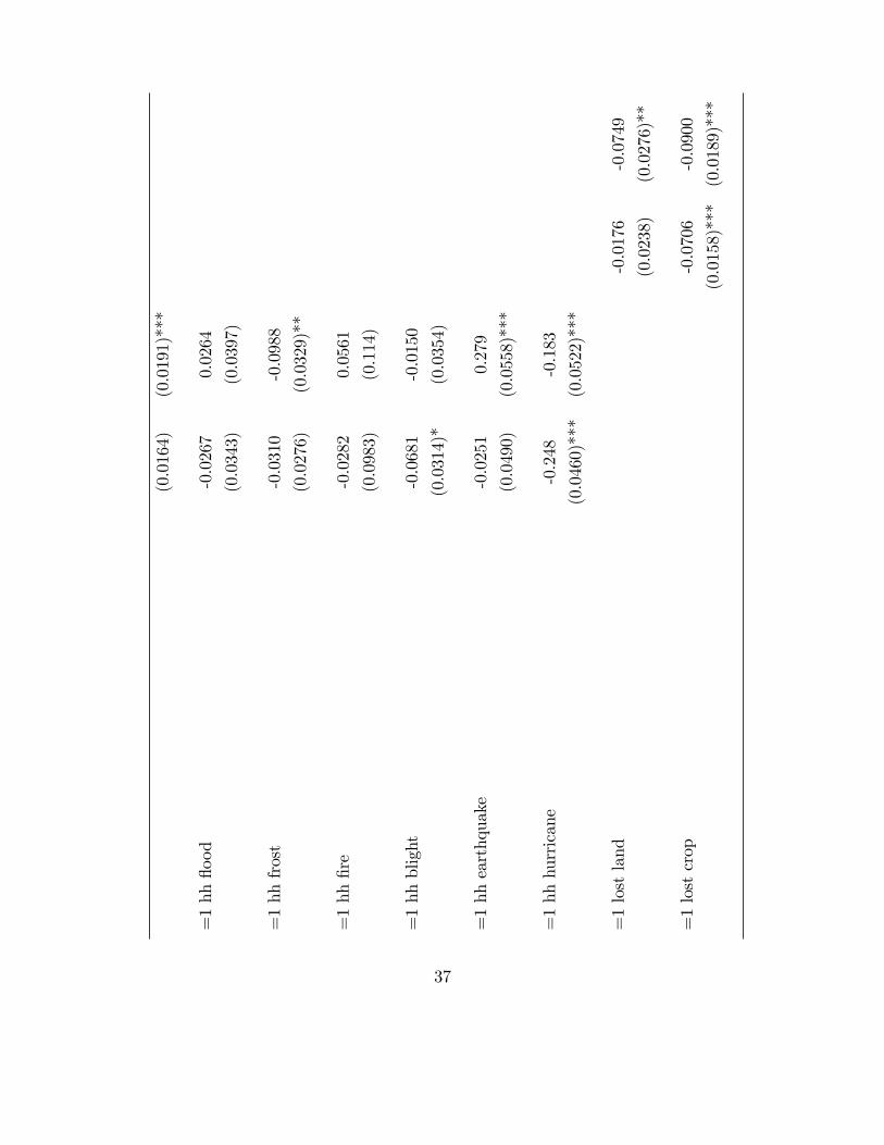
(0.0164)

(0.0191)***

=1hh�ood

-0.0267

0.0264

(0.0343)

(0.0397)

=1hhfrost

-0.0310

-0.0988

(0.0276)

(0.0329)**

=1hh�re

-0.0282

0.0561

(0.0983)

(0.114)

=1hhblight

-0.0681

-0.0150

(0.0314)*

(0.0354)

=1hhearthquake

-0.0251

0.279

(0.0490)

(0.0558)***

=1hhhurricane

-0.248

-0.183

(0.0460)***

(0.0522)***

=1lostland

-0.0176

-0.0749

(0.0238)

(0.0276)**

=1lostcrop

-0.0706

-0.0900

(0.0158)***(0.0189)***

37

=1losthouse

-0.0783

-0.0223

(0.0834)

(0.0974)

=1lostgoods

0.00210

0.158

(0.126)

(0.150)

=1deathinfam

0.360

0.532

(0.380)

(0.468)

=1lostanimals

0.127

0.125

(0.0402)**

(0.0478)**

=1hhmemberinjured

0.0922

0.125

(0.224)

(0.261)

Observations

22610

22610

22610

22610

22610

22610

AdjustedR2

0.001

-0.590

-0.592

DependentVariable:LogofHouseholdIncome

(d)fordiscretechangeofdummyvariablefrom

0to1

*p<0:05,**p<0:01,***p<0:001

38

Table5:Dorainfallshockspredictincome?

(1)

(2)

(3)

(4)

ClosestStation,vfeClosestxAN,hhfe

WeightedAverage,vfeWeightedAvxAn,hhfe

deviationfrom

the20yearmean

0.0000631

(0.0000827)

closerain,sq

-3.12e-08

(0.000000219)

closerainxan

0.0000618

(0.0000139)���

closerainxan,sq

-8.55e-08

(2.53e-08)���

weightavg,devfrom

20yr

-0.000720

(0.000153)���

weightavg,sq

0.00000187

(0.000000496)���

weighavXan

0.0000998

(0.0000217)���

weighavXan,sq

-0.000000217

(5.74e-08)���

Observations

29445

28819

29445

28819

AdjustedR2

-0.005

-0.414

-0.004

-0.415

DependentVariable:LogofHouseholdIncome,�xede¤ectsdependentonunitofanalysis

(d)fordiscretechangeofdummyvariablefrom

0to1

� p<0:05,

��p<0:01,��� p<0:001

39

Table6:RemittanceIV(A):SelfReportedShocksInstrumentedforIncome

(1)

(2)

(3)

(4)

(5)

(6)

HHshocks,fe

HHshocks,re

HHlosses,fe

HHlosses,re

Villageshocks,fe

Villageshocks,re

loghhinc

-1993.9

-850.0

-97.98

-609.2

-1231.9

-372.6

(928.2)�

(575.9)

(1071.2)

(667.1)

(559.7)�

(395.3)

imr

-7160.8

-7629.2

-8875.2

-7611.8

-7849.9

-7595.5

(1079.6)���

(656.9)���

(1167.0)���

(655.5)���

(833.3)���

(651.0)���

spousemig

3041.2

3016.8

2993.6

(414.3)���

(413.8)���

(410.3)���

numberpeopleinhh

145.1

101.7

59.44

(108.6)

(123.8)

(78.30)

numberofkidsinhh<15

-113.0

-87.33

-62.51

(75.30)

(82.65)

(60.90)

headofhheducation

55.66

55.87

56.10

(26.59)�

(26.64)�

(26.69)�

=1womanhead

84.92

111.7

138.0

(190.7)

(194.7)

(185.9)

Househaselectricity

175.0

152.6

130.4

(152.7)

(156.2)

(148.4)

percHHliterate

100.1

-1.272

-101.5

(342.6)

(372.1)

(294.3)

percHHspkSpan

-317.4

-256.6

-196.3

(226.4)

(243.5)

(198.3)

Observations

22610

15242

22610

15242

22610

15242

AdjustedR2

DependentVariable:Remittancespermigrant

(d)fordiscretechangeofdummyvariablefrom

0to1

� p<0:05,

��p<0:01,��� p<0:001

40

Table7:RemittanceIV(B):ClosestRainfallStation(deviation)InstrumentedforIncome

(1)

(2)

(3)

(4)

ClosestStation,hhfe

ClosestStation,re

ClosestxAN,hhfe

ClosestxAN,re

loghhinc

120.1

17.99

34.42

-15.39

(813.2)

(366.8)

(1101.5)

(771.9)

imr

-8813.4

-8207.8

-8792.5

-7882.6

(864.1)���

(504.7)���

(1091.8)���

(500.1)���

spousemig

2839.5

2841.8

(337.1)���

(350.5)���

numberpeopleinhh

1.936

-2.625

(63.53)

(140.7)

numberofkidsinhh<15

-16.79

-18.34

(50.95)

(98.63)

headofhheducation

40.02

39.77

(27.75)

(19.72)�

=1womanhead

171.6

124.4

(194.0)

(142.4)

Househaselectricity

84.15

73.78

(155.9)

(123.0)

percHHliterate

-206.8

-179.2

(298.2)

(343.8)

percHHspkSpan

-129.2

-109.1

(197.7)

(217.8)

Observations

29445

22069

28819

22069

AdjustedR2

DependentVariable:Remittancespermigrant,�xede¤ectsdependentonunitofanalysis

(d)fordiscretechangeofdummyvariablefrom

0to1

� p<0:05,

��p<0:01,��� p<0:001

41

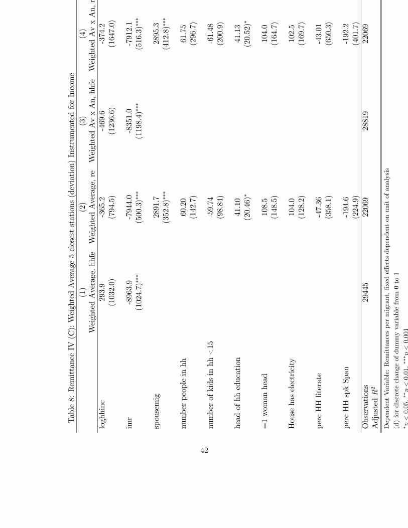
Table8:RemittanceIV(C):WeightedAverage5closeststations(deviation)InstrumentedforIncome

(1)

(2)

(3)

(4)

WeightedAverage,hhfe

WeightedAverage,re

WeightedAvxAn,hhfe

WeightedAvxAn,re

loghhinc

293.9

-365.2

-469.6

-374.2

(1032.0)

(794.5)

(1236.6)

(1647.0)

imr

-8963.9

-7944.0

-8351.0

-7912.1

(1024.7)���

(500.3)���

(1198.4)���

(516.3)���

spousemig

2891.7

2895.3

(352.8)���

(412.8)���

numberpeopleinhh

60.20

61.75

(142.7)

(296.7)

numberofkidsinhh<15

-59.74

-61.48

(98.84)

(200.9)

headofhheducation

41.10

41.13

(20.46)�

(20.52)�

=1womanhead

108.5

104.0

(148.5)

(164.7)

Househaselectricity

104.0

102.5

(128.2)

(169.7)

percHHliterate

-47.36

-43.01

(358.1)

(650.3)

percHHspkSpan

-194.6

-192.2

(224.9)

(401.7)

Observations

29445

22069

28819

22069

AdjustedR2

DependentVariable:Remittancespermigrant,�xede¤ectsdependentonunitofanalysis

(d)fordiscretechangeofdummyvariablefrom

0to1

� p<0:05,

��p<0:01,��� p<0:001

42