do fertility transitions influence infant mortality
TRANSCRIPT

PROGRAM ON THE GLOBAL DEMOGRAPHY OF AGING
Working Paper Series Do Fertility Transitions Influence Infant Mortality Declines? Evidence
from Early Modern Germany
Alan Fernihough, Mark E. McGovern
July 2013
PGDA Working Paper No. 105 http://www.hsph.harvard.edu/pgda/working.htm
The views expressed in this paper are those of the author(s) and not necessarily those of the Harvard Initiative for Global Health. The Program on the Global Demography of Aging receives funding from the National Institute on Aging, Grant No. 1 P30 AG024409-08.

Do Fertility Transitions Influence Infant Mortality Declines?
Evidence from Early Modern Germany*
Alan Fernihough� Mark E. McGovern�
July 2013
Abstract
The timing and sequencing of fertility transitions and early-life mortality declines in historical West-ern societies indicates that reductions in sibship (number of siblings) may have contributed to im-provements in infant health. Surprisingly however, this demographic relationship has received littleattention in empirical research. We outline the theoretical difficulties associated with establishingthe causal effect of sibship on infant mortality, and provide evidence on the inherent bias associatedwith conventional empirical approaches. We offer a solution that permits an empirical test of thisrelationship whilst accounting for reverse causality. Our approach is illustrated by evaluating thecausal impact of sibship on infant mortality using genealogical data from 13 German parishes span-ning the 16th, 17th, 18th and 19th centuries. Overall, our findings do not support the hypothesisthat declining fertility led to increased infant survival probabilities in historical populations.
Keywords: Demographic Transition, Family Size, Early Life Conditions, Infant Mortality
JEL Classification: D13, I15, J13, O12
The Program on the Global Demography of Aging receives funding from the National Institute on Aging,Grant No. 1 P30 AG024409-06.
Fernihough’s research is funded by the European Research Council under the European Unions SeventhFramework Programme (FP7/2007-2013) / ERC grant agreement no. 249546.
*We are grateful to Paul Devereux, Cormac O Grada, George Alter, Tommy Bengtsson, two anonymous referees, andseminar participants at Harvard and the 2013 Edinburgh FRESH meeting for helpful comments and advice.
�Institute for International Integration Studies, Trinity College Dublin. Email: [email protected].�Harvard Center for Population and Development Studies. Email: [email protected].
1

1 Introduction
The turn of the 20th century was marked by a dramatic change in Western Europe’s demographic land-
scape. This change encompassed unprecedented reductions in both fertility and mortality. A striking
feature of the mortality change was the decline in the infant death rate. That the fall in infant mortality
appeared to occur in tandem with fertility reductions suggests that these events may have been related.
Our aim is to shed light on this relationship, investigating whether reductions in fertility led to improve-
ments in infant survival. To do this, we use micro-level data collected from 13 German villages covering
the 16th, 17th, 18th, and 19th centuries.
Econometric modeling of this relationship is problematic for a number of reasons. Firstly, the measure of
fertility at an individual level, sibship, must be adjusted so that it does not induce a spurious correlation
with infant mortality. For example, the total number of children born in each household cannot be
used as a measure of sibship because this does not account for the ‘replacement effect’—where parents
have more births in order to compensate for previous child deaths. The number of surviving children
(completed net fertility) is also an inadequate measure because, by definition, this value will be lower for
families who experience a higher number of infant deaths. We derive the theoretical basis for expecting
that conventional measures of sibship provide biased results, and demonstrate that this is a substantial
problem for empirical research. A further complication is that it is not possible to observe all the
confounding variation which affects infant mortality, and therefore the estimated conditional effect of
fertility may suffer from omitted variable bias.
We propose an alternative indicator of family size: sibship at birth. This measure takes the child as the
observation unit and thus allows sibship to vary within each family. The death of older siblings are not
counted in this total, so this measure is not confounded by child replacement effects. In addition, each
child’s sibship at birth is unaffected by their fate in infancy. Because we observe the temporal ordering of
these events, this sequencing removes the potential for a structural reverse-correlation connecting infant
mortality with sibship. We acknowledge that the results of a single equation analysis may suffer from
endogeneity bias, and address this issue using an instrumental variables (IV) estimator. Our approach
instruments fertility using a measure of marital fecundity (Aguero and Marks, 2011; Klemp and Weisdorf,
2012).
Our use of historic micro-level data permits us to assess the causal importance of fertility change. There-
fore, we can evaluate whether a counterfactual fertility transition would have caused infant mortality to
fall prior to the actual fertility transition and infant mortality decline. In summary, our analysis does
not support the hypothesis that an earlier fertility transition would have caused a subsequent infant
mortality decline. Interestingly, our results may indicate the opposite, as sibship at birth is negatively
correlated to infant mortality. A one child increase in sibship at birth is associated with a moderate
reduction in infant mortality of about 1.5%. However, once we use an IV estimator to capture potential
endogeneity, we cannot reject that there is no relationship.
The remainder of this paper is structured as follows. Section 2 elaborates both our motivation and the
context for his study. In Section 3, we provide a theoretical model of fertility behavior and support our
argument for using an alternative measure of sibship by providing evidence from Monte Carlo simulations.
The fourth section introduces our data, formalizes our empirical strategy, and presents our results.
Finally, Section 5 concludes.
2

2 Context and Literature
Knodel (1974) provided a comprehensive overview of the German demographic transition.1 In 1875,
the average married couple had 5.4 surviving children, while life expectancy was roughly 37 years. By
1933, the average number of surviving children had fallen to 2.6, and mortality change contributed to
an increased life expectancy of 61.3 years—a 66% increase. The contribution of infant and childhood
mortality to the mortality decline was immense. The probability of death before the age of 15 fell from
39% to 12% and 36% to 10% for German males and females, respectively, during the period 1871–1934.
Births outside marriage averaged around 10% throughout this time period, and displayed a similar decline
to births within marriage. Marriage patterns also did not contribute much to changes in overall fertility.2
Figure 1: The Relationship Between Marital Fertility and Infant Mortality During the German Demo-graphic Transition
●
●
●
●●
●●
●
●
●
●●
●● ●
●
●
●●
●
●●
●
●
●●●●
●●
●
●
●
●
●
●
●
●
●
●
●
●
● ●
●
●
●●
●
●
●
●●
●
●
●
●
●
●●
●
●
●●
●
100
200
300
250 500 750Marital Fertility
Infa
nt M
orta
lity
Year
● 1888
1898
1908
1925
1933
Fertility and Infant Mortality, Germany 1888−1933
Source: Knodel (1974, p272 and pp288–289)
At the macro level, the extent to which these events were causally related (in either direction) is not
obvious. Figure 1 illustrates the relationship between fertility and mortality over time. In Section 3, we
discuss the importance of choosing the correct indicator of sibship when attempting to address the issue
of causality, but here we present the index of marital fertility used by the European Fertility Project to
1All statistics quoted here can be found in Knodel (1974).2For an account of changes in German economic conditions and living standards see Baten (2003).
3

document the overall association between fertility and mortality.3 There is a clear positive correlation;
regions with higher levels of infant mortality tended to have higher levels of fertility. This also holds
within a particular time period. It is also clear from this graph that both infant mortality and fertility
experienced significant falls over the period.
The literature has identified a number of potential routes through which sibship size could potentially
have influenced infant mortality in historical populations. For example, parents with fewer children
could have devoted more care and attention to their newborn. Theoretically, if family-level resources
determined infant mortality, reductions in sibship size would have improved infant survival probabilities.
In other words, we assume that finite family-level resources are positively related to infant mortality
through some (unknown) function. This is one mechanism through which we propose that fertility
affects infant survival, as a larger sibship results in a greater division of family-level inputs into the
infant-survival function. Another way in which fertility could influence infant mortality relates to the
spread of infectious diseases, as a greater number of children in any household increases the risk of
contagion.
The child resource dilution and contagion models sketched above are distinct from various forms of the
child Quantity-Quality (QQ) model originally proposed by Becker and Lewis (1973). In the child QQ
model, parents choose their optimal levels of child investment and fertility based on a given set of prices
and income. Given the dynamic nature of our question, one in which children are born after siblings
have died, we do not attempt to view our results in a child QQ framework because QQ models involve
completed fertility. In effect, our analysis measures the direct effect of fertility on infant mortality.
Figure 2 depicts a time-series of both the fertility and infant mortality transitions in historical Germany.
Two elements are worth drawing attention to. Firstly, both transitions occurred at the same time.
Knodel (1974) studied regional patterns and found that declines in fertility almost always preceded the
declines in infant mortality. This finding is important because it is inconsistent with the notion that the
infant mortality decline was an initiating factor determining the fertility decline, and also suggests that
the fertility decline may have been a component of the infant mortality transition.
Previous research suggests that economic growth played an important role in longevity improvements
(Floud et al., 2011). However, a body of literature suggests that the infant mortality decline had
alternative proximate causes than per capita income growth. For example, Bengtsson (1999) showed
that the risk of infant death was unrelated to economic changes in 18th and 19th century Sweden. Public
health initiatives are recognized as a vital source in the improvement of infant survival probabilities in the
late 19th and early 20th centuries (Delaney et al., 2011). Cutler and Miller (2005) estimated the effect
of water filtration in a number of cities in the United States during this period. Their results showed
how a large portion of this decline was caused by the implementation of policies which provided clean
water for household use. Similarly, this period was also marked by a revolution in household knowledge
surrounding germs, microbes and general cleanliness (Mokyr, 2000).
The relationship between fertility control and infant mortality has been proposed by a number of schol-
ars. For example, Woods (2000) discussed the link between the decline in infant mortality and fertility
in England and Wales, but also highlighted the problematic nature of establishing this as a causal re-
lationship with regional/macro level data, as well as the potentially confounding variation induced by
3This measure indicates the ratio of fertility compared to that of Hutterite women (the population with the highestfertility levels on record), adjusted for age distribution within childbearing ages (Knodel, 2002).
4
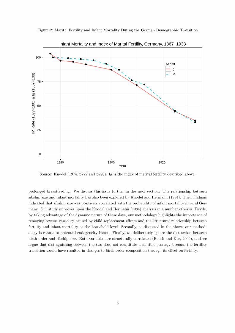
Figure 2: Marital Fertility and Infant Mortality During the German Demographic Transition
● ● ●●
●
●
●
●
●
●
●
●●
●
●
●
●
●
0
25
50
75
100
1880 1900 1920Year
IM R
ate
(187
7=10
0) &
Ig (
1867
=10
0)
Series
Ig
IM
Infant Mortality and Index of Marital Fertility, Germany, 1867−1938
Source: Knodel (1974, p272 and p290). Ig is the index of marital fertility described above.
prolonged breastfeeding. We discuss this issue further in the next section. The relationship between
sibship size and infant mortality has also been explored by Knodel and Hermalin (1984). Their findings
indicated that sibship size was positively correlated with the probability of infant mortality in rural Ger-
many. Our study improves upon the Knodel and Hermalin (1984) analysis in a number of ways. Firstly,
by taking advantage of the dynamic nature of these data, our methodology highlights the importance of
removing reverse causality caused by child replacement effects and the structural relationship between
fertility and infant mortality at the household level. Secondly, as discussed in the above, our method-
ology is robust to potential endogeneity biases. Finally, we deliberately ignore the distinction between
birth order and sibship size. Both variables are structurally correlated (Booth and Kee, 2009), and we
argue that distinguishing between the two does not constitute a sensible strategy because the fertility
transition would have resulted in changes to birth order composition through its effect on fertility.
5
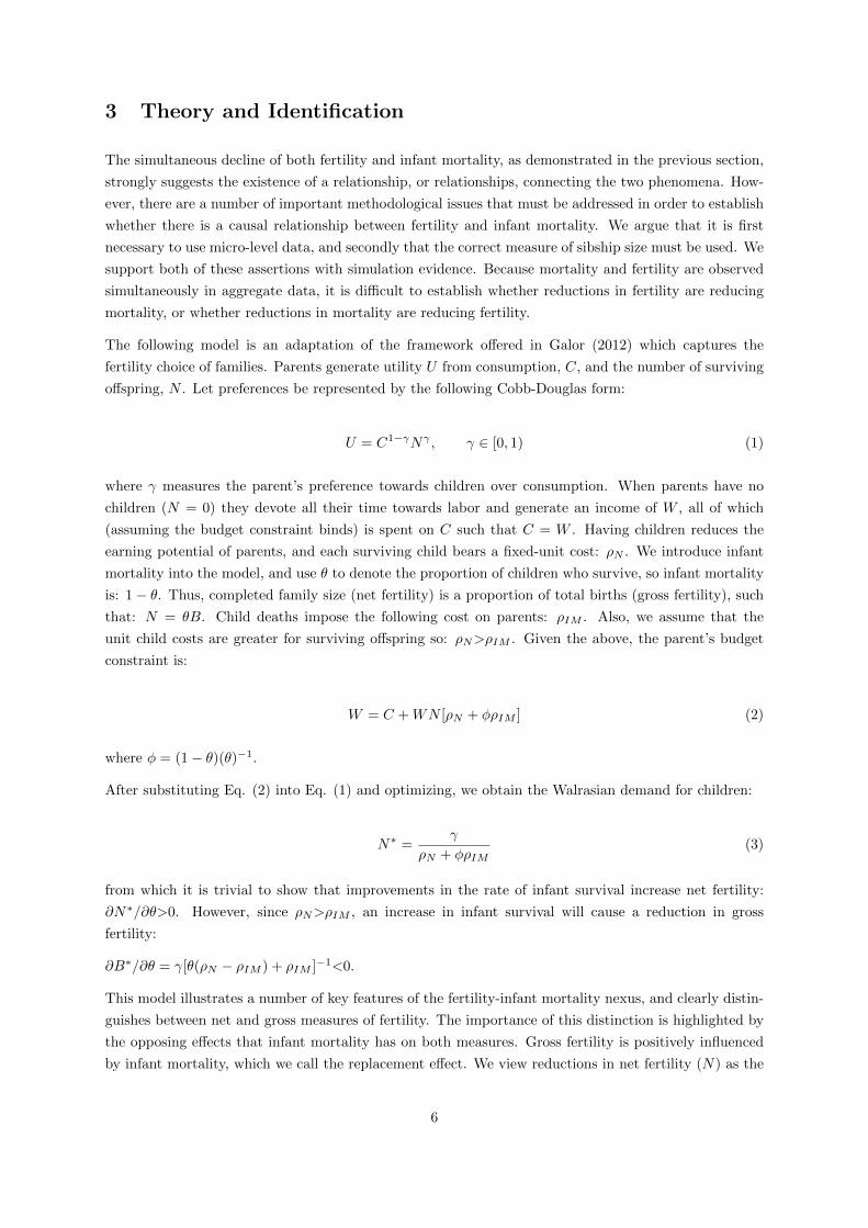
3 Theory and Identification
The simultaneous decline of both fertility and infant mortality, as demonstrated in the previous section,
strongly suggests the existence of a relationship, or relationships, connecting the two phenomena. How-
ever, there are a number of important methodological issues that must be addressed in order to establish
whether there is a causal relationship between fertility and infant mortality. We argue that it is first
necessary to use micro-level data, and secondly that the correct measure of sibship size must be used. We
support both of these assertions with simulation evidence. Because mortality and fertility are observed
simultaneously in aggregate data, it is difficult to establish whether reductions in fertility are reducing
mortality, or whether reductions in mortality are reducing fertility.
The following model is an adaptation of the framework offered in Galor (2012) which captures the
fertility choice of families. Parents generate utility U from consumption, C, and the number of surviving
offspring, N . Let preferences be represented by the following Cobb-Douglas form:
U = C1−γNγ , γ ∈ [0, 1) (1)
where γ measures the parent’s preference towards children over consumption. When parents have no
children (N = 0) they devote all their time towards labor and generate an income of W , all of which
(assuming the budget constraint binds) is spent on C such that C = W . Having children reduces the
earning potential of parents, and each surviving child bears a fixed-unit cost: ρN . We introduce infant
mortality into the model, and use θ to denote the proportion of children who survive, so infant mortality
is: 1− θ. Thus, completed family size (net fertility) is a proportion of total births (gross fertility), such
that: N = θB. Child deaths impose the following cost on parents: ρIM . Also, we assume that the
unit child costs are greater for surviving offspring so: ρN>ρIM . Given the above, the parent’s budget
constraint is:
W = C +WN [ρN + φρIM ] (2)
where φ = (1− θ)(θ)−1.
After substituting Eq. (2) into Eq. (1) and optimizing, we obtain the Walrasian demand for children:
N∗ =γ
ρN + φρIM(3)
from which it is trivial to show that improvements in the rate of infant survival increase net fertility:
∂N∗/∂θ>0. However, since ρN>ρIM , an increase in infant survival will cause a reduction in gross
fertility:
∂B∗/∂θ = γ[θ(ρN − ρIM ) + ρIM ]−1<0.
This model illustrates a number of key features of the fertility-infant mortality nexus, and clearly distin-
guishes between net and gross measures of fertility. The importance of this distinction is highlighted by
the opposing effects that infant mortality has on both measures. Gross fertility is positively influenced
by infant mortality, which we call the replacement effect. We view reductions in net fertility (N) as the
6

most important aspect of the fertility decline. Therefore, the positive influence of infant mortality on
net fertility predicted by the model is inconsistent with the hypothesis that the fertility transition was
partially caused by reductions in infant mortality. A similar conclusion was reached by Doepke (2005),
who analyzed a series of more complex fertility choice models.
Theoretically, the positive relationship between infant mortality and net fertility strengthens our moti-
vation for examining whether fertility determined infant mortality. Thus, we extend the model to permit
endogenous infant mortality, so that fertility has a negative impact on infant survival. However, both
B and N are completed measures of fertility which are ambiguously related to infant mortality, and as
such we argue that the inclusion of endogenously determined infant mortality requires an extension of
the framework to incorporate the sequential discrete-time process jointly associated with both family
formation and infant mortality.
More formally, whether an individual child i from family j lives or dies assumes a binary value, determined
by an as of yet undefined function: dij = 1{fij(•)>0}. Thus, the completed infant survival coefficient θj
for the jth family is derived from discrete-time process:
θj = 1−∑Bj
i=1 dijBj
=Nj +
∑Bj
i=1 dijNj
. (4)
Eq. (4) underlines the problematic nature of using completed fertility measures, as both the replacement
effect, driven by Bj , and the structurally induced net correlation, driven by Nj , can cause changes in in
θj independently of the term determining infant mortality, dij . Therefore, it is apparent that modeling
the effect of fertility on infant mortality involves modeling dij = 1{fij(•)>0}, such that the function
fij(•) incorporates an individual or time specific measure of fertility.
We propose sibship size at birth for the ith child in family j (nij = [Bj − i]−∑i−1k=1 dk) as the measure
through which fertility influences infant mortality. To the best of our knowledge this is the first use of this
measure of sibship as the economics literature has focused exclusively on completed sibships (for example
Black et al., 2005). The sibship at birth measure is consistent with the sequential discrete-time ordering
associated with family level demographic patterns. We can summarize our argument as follows. If infant
mortality is the outcome of interest, then we argue that the only appropriate measure of sibship to use is
sibship at birth. It is hard to see why a completed sibship measure should be related to infant survival.
For example, suppose that an individual has 2 siblings at birth, but has 10 siblings at age 15. It is not
clear how any event which occurs after the age of 1 (in this case the birth of additional siblings) could
affect whether the individual survived their first year or not, especially in a model of resource dilution.
Finally, because we observe these events sequentially in our data, at the individual level a person’s fate
in infancy cannot affect their sibship at birth, thereby removing the structural reverse correlation which
generally connects infant mortality with an alternative measure of sibship. When we observe a birth in
these data, we are able to establish the number of living siblings, which we then hold constant. Following
this, we observe whether the individual suffered an infant death. So we measure our outcome (mortality),
after our ‘treatment’ (sibship) is fixed.
A prototypical regression model capturing the influence of sibship on infant mortality is:
dij = α+ βnij + εij (5)
7

where dij is the same as Eq. (4), nij is net sibship for child i in family j, β is the parameters of interest,
and εij is introduced to add uncertainty, or a random component, to infant mortality. In the proceeding
section we apply (a modified version of) the model in Eq. (5) to empirically test the hypothesis that
sibship size at birth was an important determinant of infant mortality (β>0). However, we use the
remainder of this section to illustrate how using alternative measures of fertility leads to biased results.
To demonstrate the consequences which arise from the use of incorrect regressors on the right-hand side
of Eq. (5), we perform a Monte-Carlo simulation analysis, that features all of the main components
from the theoretical insights offered in the preceding analysis. In addition, we also augment a number
of these components, and introduce a number of stochastic processes—the importance of which has
been emphasized in previous research (Kalemli-Ozcan 2003). The introduction of this random variation
provides a richer, and more realistic platform, from which we base our comparisons of the potential
econometric methodologies. The technical details of our simulation are provided in an appendix.
We expect the model that uses net sibship at birth as the regressor to correctly identify the effect. Other
net fertility measures include a completed sibship variable, and an aggregated or macro type measure.
Estimation was performed for both net and gross measures of all fertility variables and we also perform
an analysis that is equivalent to using sibship at birth, except we include family fixed effects. This is
a potentially desirable specification because the fixed effects remove all family-level variation that may
threaten identification. However, estimation via the fixed-effects model is problematic. The reason for
this is that fixed-effects estimators make comparisons within each group as defined by the fixed-effects
specification. In our case, this comparison is made within each family. However, the within comparison
of siblings is invalid as the death of one sibling mechanically reduces the net sibship for the surviving
siblings. This indicates that we would expect to find a spurious positive association connecting net
sibship at birth and infant mortality.
We begin this analysis by comparing the output produced in the eight models discussed in the above,
setting β = 0. To generate our data, we run the simulation procedure described in the appendix
to produce 100 family level observations in 100 macro/village level units. We repeat this 100 × 100
simulation procedure 100 times, performing the eight regression models for each repetition. Figure 3,
demonstrating density plots of the estimates, provides an illustration of the results when we set β = 0.
From this figure, it is apparent that the net fertility at birth measure is correctly identifying β. On
average, the gross fertility at birth with family fixed effects and net macro measures also appear to
correctly estimate β. All of the other models yield an evidently biased β estimate.
The next part of this analysis evaluates the eight models where β = 0.03. In other words, the marginal
effect from an extra sibling at birth increases the probability of infant death by 3%. Repeating the
simulation method outlined in the above permits us to once again examine the efficacy of our eight
models. The results of this analysis are displayed in Figure 4 and once again illustrate how the net
sibship at birth fertility measure correctly identifies the parameter of interest.4 Additionally, Figure 4
also shows how the gross fertility measure with family fixed effects and the net macro measure of net
fertility are biased in this setting, while the other models once again produce similar biases. This result
is in line with our predictions regarding the replacement effect, the structural net correlation, and the
inclusion of family fixed effects.
4The distribution of the sibship at birth estimator does not peak exactly at 0.03. The reason for this is that we usea linear probability model (LPM), and we acknowledge that this estimator is known to be both biased and inconsistent(Horrace and Oaxaca 2006). However, the bias here is almost negligible, therefore justifying our use of the LPM, inparticular since the LPM is computationally more efficient in this exercise.
8

Figure 3: Measuring the Effects of Sibship with no True Relationship, β = 0
At Birth At Birth Fixed Effects
Completed Macro
0
100
200
300
400
0
200
400
0
100
200
300
400
0
25
50
75
−0.02 −0.01 0.00 0.01 0.02 0.03 −0.02 −0.01 0.00 0.01 0.02 0.03Effect Size
Den
sity
Fertility Gross Net
Figure 4: Measuring the Effects of Sibship with a Relationship, β = 0.03
At Birth At Birth Fixed Effects
Completed Macro
0
100
200
300
400
500
0
100
200
300
400
0
100
200
300
400
0
25
50
75
100
−0.02 0.00 0.02 0.04 0.06 −0.02 0.00 0.02 0.04 0.06Effect Size
Den
sity
Fertility Gross Net
4 Empirical Analysis
4.1 Data
This study uses historical genealogies from 13 German villages which span the onset of the demographic
transition. The evidence presented in the previous section supports the arguement that this type of life
9

history data allow us to answer questions of causality in a manner which is not possible with aggregate
statistics. These data are obtained from parish records which contain details of the major events for all
families in that particular locality. Demographic information pertaining to parents and children (such
as dates of birth and marriage) are included, as well as measures of socioeconomic status (parental
occupation) and health (age at death), all over the course of multiple generations.
The written parish records began to be collated in the early part of the 20th century, as part of a
project to document genealogy in each locality throughout Germany. This project was interrupted with
the outbreak of the Second World War, and consequently these data are only available for a limited
number of parishes. These villages were therefore not intended to be a representative sample of the
German population, however subsequent verification exercises have suggested that the quality of these
genealogies is high, as they also match up well with the available registration data (Knodel, 2002).
A limited number of papers (for example Klemp and Weisdorf, 2012) have examined the effects of
sibship using Anglican records collected from 26 parishes in England. Cohort studies have also been
used in researching this topic, including Boyd-Orr (Frijters et al., 2010) and the Swedish Uppsala Birth
Cohort Study (Modin, 2002). In our case these data have a number of advantages. Specifically, the
quality of the reconstruction, the comprehensive multi-generational nature of the database, and the fact
that the genealogies span the beginning of the demographic transition in Germany. Our empirical data
contain information on the factors that we expect may confound the fertility-infant mortality relationship.
These variables includes parents’ age at birth and place of birth. Additionally, we are able to control
for a number of typically unobserved variables, including measures of parental health and socioeconomic
status. These control variables reduce the risk of a confounder inducing selection into both large families
and high mortality.
However, while we can control for these factors, we cannot definitively rule out the possibility that vari-
ation from some omitted source may simultaneously affect infant mortality and fertility. Examples of
these include measures of parenting “quality”, or breastfeeding (Brown and Guinanne, 2001). Breast-
feeding is an important determinant of both fertility and infant mortality (Knodel, 2002). Extended
breastfeeding acts as a form of contraception, and thus lengthens birth intervals with the consequence of
reducing gross fertility. In historical populations, a premature cessation of breastfeeding could increase
the hazard of infant death substantially, since it exposed vulnerable infants to potentially contaminated,
and therefore unhygienic, food sources. Thus, breastfeeding is an example of a variable which would
bias the relationship between sibship and mortality upwards. Alternatively, net sibship itself could also
represent a measure of maternal or paternal ability. Thus, a bigger net sibship at birth may capture
the fact that some parents are better able to carry babies to term and help them survive, and that
this reproductive success is transmitted intergenerationally though a combination of environmental or
genetic endowments. This is an example of an omitted variable which would bias the effects of sibsize
downwards. It is difficult to determine a priori which effect would dominate. We return to this issue
when discussing our results.
Fortunately, it is easier to identify plausibly exogenous sources of fertility differences at the individual
level than it is at the macro level. If we observe variation in sibship which is unrelated to potential
confounders, this can be used to obtain a consistent estimate of the effects of sibship size on mortality.
We adopt the approach proposed in Aguero and Marks (2011), and also used in Klemp and Weisdorf
(2012). We take advantage of the fact that there is a random component to natural fertility, in the
sense that some couples are more ‘biologically compatible’, and find it easier to conceive than others.
10

Aguero and Marks (2011) highlight the fact that the epidemiology literature on the subject has found
surprisingly few robust predictors of this natural fecundity. For example, biological fertility has been
found to be unrelated to family background characteristics (Joffe and Barnes, 2000), as well as lifestyle
factors and behavior (Buck et al., 1997). This is important, as the identifying assumption is that the
instrument (in this case natural fertility) should affect the outcome (infant mortality) only through its
effect on sibship. As in Klemp and Weisdorf (2012), we take the length of time between marriage and
first birth (standardized for the mother’s age at marriage) as our indicator of natural fecundity.5 We
find that it is strongly predictive of sibship, so couples who conceived soon after getting married appear
to have been more compatible biologically, and went on to have larger families.
Figure 5: Village Locations
Middels Werdum
BraunsenHoeringhausenMassenhausenVasbeck
GrafenhausenHerbolzheimRust
Oeshelbronn
Gabelbach
Anhausen
Kreuth
Location of 13 German Villages from Knodel Data
The main disadvantage of using these data relates to the extent to which it is possible to generalize from
these particular 13 German villages. However, the trajectories for both infant mortality and fertility
were similar across regions and type of location (urban and rural localities). Furthermore, as is shown
in Figure 5, the villages are relatively geographically dispersed, and incorporate important variation
such as religion, and economic and social structures. Therefore, while these data tell a rural story, it is
reasonable to assume that our results have wider implications.
5This variable is standardized using the residuals from a regression estimating the predicted number of days frommarriage to the first birth date, controlling for age at marriage. We use a quadratic in age at marriage, however using ahigher order polynomial or a semi-parametric model does not affect the results.
11

4.2 Summary Statistics
A number of papers have used these German parish register data, particularly in the historical demogra-
phy literature. This research stems from a series of contributions by Knodel who was among the first to
popularize the analysis of this data source. Much of this research is collected in Knodel (2002). Summary
statistics for the analysis sample are presented in Table 1.
Table 1: Summary Statistics
Variable Obs Mean Std. Dev. Min Max
Infant Death 47,665 0.203 0.402 0.000 1.000Stillbirth 47,665 0.023 0.151 0.000 1.000Sibship at Birth 47,665 1.889 1.699 0.000 8.000Completed Sibship (Gross) 47,665 5.963 3.087 0.000 18.000Male 47,665 0.514 0.500 0.000 1.000Year/100 47,665 18.169 0.560 15.910 18.990(Year/100)2/100 47,665 0.330 0.020 0.253 0.361Mother’s Age at Birth/100 42,539 0.315 0.061 0.148 0.542Father’s Age at Birth/100 40,525 0.356 0.076 0.150 0.770Mother’s Age at Death/100 40,404 0.609 0.152 0.184 0.986Father’s Age at Death/100 38,789 0.641 0.136 0.207 0.979Mother Survived until the Age of 40 42,796 1.000 0.000 1.000 1.000Parent with Missing Vital Record Dates 34,171 1.000 0.000 1.000 1.000Time Till First Birth 30,080 480.899 352.876 270.000 6855.000Time Till First Birth— 26,644 -0.186 0.938 -1.224 17.134Orthogonal to Mother’s Age at Marriage
Occupation Obs % Village Obs %
Artisan 9,755 20.466 Anhausen 1,350 2.832Businessman 3,331 6.988 Braunsen 1,150 2.413Cottager 3,238 6.793 Gabelbach 1,331 2.792Civil Servant 369 0.774 Grafenhausen 5,684 11.925Farmer 14,263 29.923 Herbolzheim 9,879 20.726Home Industry 759 1.592 Hoeringhausen 2,703 5.671Kneckt 563 1.181 Kreuth 765 1.605Labourer 1,264 2.652 Massenhausen 1,968 4.129Professional 860 1.804 Middels 2,918 6.122Unknown 2,069 4.341 Oeshelbronn 4,996 10.481Rural Labourer 3,129 6.565 Rust 7,390 15.504Soldier 232 0.487 Vasbeck 2,469 5.180Tenant Farmer 228 0.478 Werdum 5,062 10.620Unskilled 396 0.831Weaver 2,411 5.058None 3,649 7.656Legal Status 714 1.498Honorary Title or Position 435 0.913
The summary statistics displayed in Table 1 provide an overview of both the variables used in our
empirical exercise, and potentially missing data. On average, infant mortality afflicted about 20% of all
observations. Around 2% of the sample were stillborn, and we have also included these in the Infant
Death variable. Our sibship at birth variable was constructed by taking account of all births, deaths, and
the timing of these events in each relevant family. To capture maturity, as we might expect older children
to exit the household or start to contribute towards the household’s income, we assume that children no
longer matter for sibship at birth upon reaching the age of 15. The completed sibship variable measures
how many births have occurred in each household. We divide a number of our variables by 100. This
aids an interpretation of the regression coefficients presented later. The maximum year is 1899, as we
do not consider the small number (2,264) of observations born in the 20th century because there are no
marriages after this date in these data.
12

Each of the parent’s age variables indicate the potential for missing data. To highlight these numbers we
have created an indicator showing if at least one of these variables is missing for an observation: Parent
with Missing Vital Record Dates. Thus, we see that 34,171 of the observations contain the complete set of
parental vital date measures. Table 1 also displays the potential for missing data in our marital fecundity
measure: Time Till First Birth. This variable cannot be constructed for pre-marital conceptions. Thus,
we do not consider observations where a birth occurs in under 270 days of the marriage date. A similar
restriction is advised in Klemp and Weisdorf (2012). Since mother’s age at marriage is highly correlated
with the time till first birth measure, we construct a orthogonalized measure, as described in footnote 5.
However, since this measure requires the mother’s age at marriage, there are slightly fewer observations
where this variable is available. Another restriction, recommended by Knodel (2002), is to focus on
families where the mother has survived until at least reaching the menopause, and hence not curtailing
any opportunity to have a larger family. We set a low bound of 40 for the age at menopause, although
setting a higher bound does not alter our results. Table 1 indicates that this restriction only applies
to a minority of our data sample. We evaluate the sensitivity of our results to sample selection in the
following analysis.
4.3 Empirical Results
We begin our formal analysis by implementing regression models that control for observable characteris-
tics. As outlined above, our data allow us to control for parental health and socioeconomic status, which
are likely to be the most important confounding variables. We estimate the following linear probability
model for infant mortality:6
IMi = Xiβ + SSABiγ + εi (6)
where the event of infant death (IMi—with individuals denoted i), is a function of sibship size at birth
(SSABi), and a number of other control variables (Xi). Our main parameter of interest is γ, the effect
of sibship size at birth on the probability of infant mortality. Results from this model are presented in
Table 2.
The coefficients in Table 2 display how sibship at birth affects infant mortality across a variety of
specifications. We examine how robust this effect is by introducing additional control variables, and
placing additional restrictions on our sample. Overall, these results run counter to our prior expectation
as sibship at birth appears to have a negative on infant mortality. In each of the five specifications, we
find that sibship at birth reduces the likelihood of infant death. This effect strengthens once controls are
introduced in our preferred specifications. However, we do not find that the magnitude of this correlation
reduces with the inclusion of additional controls or further sample restrictions, shown in columns (3) to
(5). These results indicate that an additional sibling at birth will reduce the probability of death by
around 1.5%. One possible mechanism through which this effect operates is experience—as both bringing
a child to term and ensuring that it survives the first year of life represents a skill. In other words, we
can think of this as a learning-by-doing process whereby sibship at birth represents the parent’s ability
in keeping their offspring alive. Therefore, a larger sibship at birth, a net measure of fertility, will be
indicative of the parent’s success in this regard. This effect is conditional on parent’s age at birth, so this
explanation is robust to the alternative hypothesis that this is a pure age effect for parents. Irregardless,
our finding of a negative correlation is not consistent with the theory that fertility reductions played a
role in the decline of infant mortality.
6Our results are robust to using the probit model.
13

Table 2: Infant Mortality and the Effect of Sibship at Birth: OLS Regressions
OLS OLS OLS OLS OLS(1) (2) (3) (4) (5)
Sibship at Birth -0.003*** -0.013*** -0.014*** -0.014*** -0.017***(0.001) (0.002) (0.002) (0.002) (0.002)
Male 0.031*** 0.033*** 0.033*** 0.034*** 0.033***(0.004) (0.004) (0.004) (0.005) (0.006)
Year/100 0.179 0.146 0.704*** 0.605** 0.808**(0.195) (0.266) (0.271) (0.280) (0.345)
(Year/100)2/100 -3.275 -2.239 -17.576** -15.016* -20.832**(5.434) (7.361) (7.492) (7.751) (9.555)
Mother’s Age at Birth/100 0.560*** 0.483*** 0.471*** 0.549***(0.061) (0.061) (0.064) (0.078)
Father’s Age at Birth/100 0.067 0.147*** 0.143*** 0.165***(0.048) (0.047) (0.051) (0.064)
Mother’s Age at Death/100 -0.198*** -0.183*** -0.097*** -0.089***(0.018) (0.018) (0.023) (0.029)
Father’s Age at Death/100 -0.013 -0.030 -0.020 -0.046*(0.020) (0.019) (0.021) (0.026)
Father’s Occupation N Y Y Y YVillage Fixed Effects N N Y Y YMother Survived until the Age of 40 N N N Y YTime Till First Birth >269 N N N N YObservations 47,665 34,171 34,171 30,442 18,878
*** p<0.01, ** p<0.05, * p<0.1. Clustered, at the family level, standard errors in parentheses.
Table 3: Infant Mortality and the Effect of Completed Sibship (Gross): OLS Regressions
OLS OLS OLS OLS OLS(1) (2) (3) (4) (5)
Completed Sibship (Gross) 0.009*** 0.012*** 0.010*** 0.011*** 0.011***(0.001) (0.001) (0.001) (0.001) (0.001)
Male 0.031*** 0.033*** 0.033*** 0.034*** 0.034***(0.004) (0.004) (0.004) (0.005) (0.006)
Year/100 0.142 0.167 0.640** 0.535* 0.622*(0.191) (0.260) (0.267) (0.274) (0.340)
(Year/100)2/100 -2.306 -2.725 -15.711** -12.985* -15.425(5.311) (7.183) (7.390) (7.586) (9.407)
Mother’s Age at Birth/100 0.406*** 0.327*** 0.330*** 0.385***(0.055) (0.055) (0.058) (0.071)
Father’s Age at Birth/100 -0.015 0.061 0.056 0.059(0.047) (0.047) (0.050) (0.063)
Mother’s Age at Death/100 -0.228*** -0.211*** -0.094*** -0.085***(0.018) (0.018) (0.023) (0.029)
Father’s Age at Death/100 -0.050** -0.060*** -0.059*** -0.085***(0.020) (0.019) (0.021) (0.027)
Father’s Occupation N Y Y Y YVillage Fixed Effects N N Y Y YMother Survived until the Age of 40 N N N Y YTime Till First Birth >269 N N N N YObservations 47,665 34,171 34,171 30,442 18,878
*** p<0.01, ** p<0.05, * p<0.1. Clustered, at the family level, standard errors in parentheses.
14

In contrast to the results in Table 2, all of the fertility—Completed Sibship (Gross)—coefficients in
Table 3 are positive. Clearly, this is the result we would expect to obtain considering the replacement
effect. In other words, reverse causality is at play here and the number of births for a family will be
higher for families that experience infant mortality as they ‘replace’ these children. Like in Table 2,
the coefficients, although biased, are remarkably stable across each of the five specifications. Table 3
underlines our motivation for using sibship at birth as our measure of fertility, and is consistent with our
simulation results.
Table 4: Infant Mortality and the Effect of Sibship at Birth: IV Regressions
Sibship at Birth Infant Mortality Sibship at Birth Infant MortalityFirst Stage First Stage
OLS TSLS OLS TSLS(1) (2) (3) (4)
Sibship at Birth -0.007 -0.014(0.011) (0.012)
Time Till First Birth—Orthogonalized -0.293*** -0.297***(0.021) (0.023)
Male 0.003 0.033*** 0.005 0.033***(0.018) (0.006) (0.019) (0.006)
Year/100 -2.541 0.884*** -2.530 0.815**(1.822) (0.338) (1.931) (0.347)
(Year/100)2/100 65.238 -22.638** 65.242 -21.016**(50.548) (9.333) (53.579) (9.602)
Mother’s Age at Birth/100 12.256*** 0.444*** 12.163*** 0.514***(0.363) (0.151) (0.387) (0.157)
Father’s Age at Birth/100 4.532*** 0.109 4.452*** 0.152*(0.333) (0.076) (0.361) (0.080)
Mother’s Age at Death/100 0.031 -0.189*** -0.071 -0.089***(0.121) (0.022) (0.173) (0.029)
Father’s Age at Death/100 0.115 -0.058** 0.035 -0.046*(0.141) (0.025) (0.155) (0.027)
Father’s Occupation Y Y Y YVillage Fixed Effects Y Y Y YMother Survived until the Age of 40 N N Y YTime Till First Birth >269 Y Y Y YFirst-Stage Partial F-Statistic 191.75 165.65Observations 21,264 21,264 18,878 18,878
*** p<0.01, ** p<0.05, * p<0.1. Clustered, at the family level, standard errors in parentheses.
These data allow us to control for a number of observable characteristics. Nevertheless, we are still
concerned that some unobservable factor, like breastfeeding, could be simultaneously correlated with
both infant mortality and sibship at birth. Table 4 demonstrates the results of an analysis that captures
potential omitted variables bias. Here we use an instrumental variables (IV) estimator with our marital
fecundity variable. A further discussion on the validity of this variable as an instrument for fertility
is provided in the text below. We perform two two-stage least-squares (TSLS) regressions, reporting
both the first-stage, columns (1) and (3), and second-stage, columns (2) and (4), results.7 Here we are
stratifying our analysis based on whether the mother of the individual survived until 40, although our
results appear to be consistent regardless of the specification.
7Once again, we obtain almost identical results when using a Probit IV estimator in the spirit of Rivers and Vuong(1988). We have also considered Generalised Additive Models (Wood, 2000) which allow for non-linear effects of sibship,including in the presence of endogeneity (Marra and Radice, 2011). We reach the same conclusions as for the linear effectmodels.
15

Both first-stage regressions indicate that our martial fecundity variable—time till first birth—is highly
correlated with fertility. The first-stage partial F-statistics, 191.75 and 165.65, are well in excess of the
conventional weak instrument threshold level. Thus, this instrument satisfies one of the key assumptions
regarding IV methodology, that the IV is sufficiently correlated with the endogenous regressor. Our
findings in Table 4 are somewhat mixed. On one hand, the sibship at birth coefficients tally well with
the equivalent effects displayed in Table 2. The coefficients are both negative and of a similar magnitude.
On the other hand, these IV estimates are a lot less precise compared to the OLS equivalents in Table 2.
Consequently, the standard errors on the sibship at birth variable are lot larger, and the t-test statistics
are much below any conventional level regarded to claim statistical significance.
Overall, the IV results in Table 4 present ambiguous evidence on the hypothesis that sibship at birth and
infant mortality were negatively related. Irregardless, these results, like those in Table 2, do not support
the hypothesis that historic falls in infant mortality were caused by the fertility decline. If anything,
these results may indicate that a counterfactual fertility transition would have caused infant mortality
to rise. One mechanism that may lie behind this claim is that increased net fertility provides parents
with more opportunities to learn about infant care, and therefore the infant mortality probability falls
with the number of ‘successes’ that parent’s have in raising their children. However, given the size of
the standard errors in Table 4, we must refrain from placing too much emphasis on this finding as we
cannot reject the hypothesis that fertility and infant mortality are unrelated.
The validity of the results in Table 4 are conditional on the instrument meeting the exclusion restriction.
Namely, our measure of marital fecundity must only affect infant mortality through its impact on sibship
at birth. If families with lower net fertility also differ in terms of some other factor influencing infant
mortality, then the exclusion restriction is not satisfied and our IV results could be biased. For example,
maternal health could affect both fertility and child health. Our argument is that marriage generally
signaled the desire to start a family and conceive during this time period, and therefore the time between
the marriage date and the date of the first birth represents a measure of natural fertility which has been
found to be mainly exogenous in the literature (Joffe and Barns, 2000; Buck et al., 1997). However,
it is important to provide some test of whether this is a reasonable assumption in this context. Table
5 demonstrates that the instrument has no predictive power for either maternal longevity, or infant
mortality of the first born. If time till first birth was affected by maternal health, we would expect it to
predict life expectancy of the mother, however this is not the case. Secondly, suppose some parents had
lower desired fertility (which also affected infant mortality), and therefore had greater time to first birth,
then we would expect time to first birth to affect the mortality of the first born. This is an important
test as clearly all firstborns have the same sibship.8 As with maternal mortality, there is no evidence that
the instrument affects this outcome. We therefore conclude that the exclusion restriction is plausible in
our application.9
8We thank a referee for this valuable suggestion.9We have also performed an equivalent analysis with the elapsed time between the first and second births. This variable
fails the instrument validity test.
16

Table 5: Test of Instrument Validity, Time Till First Birth—Orthogonalized
Mother’s Age at Mother’s Age atDeath/100 Death/100 Infant Mortality Infant Mortality
OLS OLS OLS OLS(1) (2) (3) (4)
Time Till First Birth—Orthogonalized 0.001 0.001 0.001 0.005(0.002) (0.001) (0.005) (0.006)
Year/100 -0.670*** -0.735*** 2.148*** 2.276***(0.228) (0.179) (0.564) (0.575)
(Year/100)2/100 19.554*** 21.581*** -58.523*** -62.365***(6.331) (4.954) (15.642) (15.948)
Mother’s Age at Birth/100 0.294*** 0.011 0.488*** 0.471***(0.050) (0.041) (0.142) (0.152)
Father’s Age at Birth/100 -0.030 -0.034 0.136 0.136(0.037) (0.031) (0.102) (0.108)
Father’s Age at Death/100 0.105*** 0.074*** -0.048 -0.036(0.018) (0.014) (0.043) (0.047)
Male 0.044*** 0.043***(0.012) (0.013)
Mother’s Age at Death/100 -0.193*** -0.067(0.039) (0.055)
Father’s Occupation Y Y Y YVillage Fixed Effects Y Y Y YMother Survived until the Age of 40 N Y N YTime Till First Birth >269 Y Y Y YObservations 4,296 3,602 4,296 3,602
*** p<0.01, ** p<0.05, * p<0.1. Robust standard errors in parentheses.
5 Conclusions
All developed nations have undergone dramatic changes in fertility, which tended to be accompanied by
equally dramatic reductions in mortality. The sequencing of these two events within countries is almost
always suggestive of interdependency; however there has been surprisingly little research examining the
causal relationship between these two demographic phenomena. A potential explanation for this absence
is that the types of aggregate data which tend to be most readily available for analysis are plagued by
the problem of reverse causality. In this paper, we present our case that individual level data, which
allow for the temporal ordering of mortality and fertility, are required to address this issue.
We discuss the bias inherent in conventional measures of fertility. We present evidence from a theoretical
model of fertility choice, as well as evidence from simulated data which supports the use of sibiship
at birth as the only appropriate indicator of fertility. Since sibship at birth does not include previous
deaths, we account for the so-called replacement effect. In addition, this measure is unaffected by the
individual’s fate in infancy, removing the structural reverse-correlation connecting infant mortality to
sibship. Essentially, as we observe the person’s sibship at birth first, and then whether they died in
infancy or not, we can use this sequential timing to address reverse causality.
We also address potential omitted variable bias by instrumenting for sibship with a measure of natural
fertility that has been used previously as a source of exogenous variation in sibship (Aguero and Marks,
2011; Klemp and Weisdorf, 2012). This approach accounts for the possibility that parents may select
to have higher fertility on the basis of some unobserved characteristic which is correlated with risk of
mortality (such as some form of parental quality).
17

To empirically evaluate the impact of a counterfactual fertility transition in a historical population, we
use micro-level data from German parish records that span the 16th, 17th, 18th and 19th centuries. The
results from our empirical models do not support the hypothesis that fertility transitions influence infant
mortality declines. In fact, our results appear to indicate the opposite—that infant mortality would have
increased in response to a reduction in net fertility. However, our IV effect estimates are quite imprecise,
and we would caution any definitive interpretation regarding this negative effect. Thus, we conclude that
declining fertility had little effect on infant mortality, despite the suggestive timing of these two events
in Germany, and elsewhere. Furthermore, we also demonstrate how the effects of sibship cohorts are
substantially biased upwards when using completed sibship to value fertility.
Our results have a number of consequences. Our conclusion that infant mortality was not affected
by the fertility transition stands in contrast to previous research which has relied on macro data (e.g.
Galloway et al., 1998). We highlight the importance of choosing the correct measure of sibship. Many
developing nations are currently in the midst of undergoing a similar reduction in fertility, and an
interesting extension of this research would be to address whether the results obtained in this paper can
be extended to this contemporary context.
18

References
Aguero JM, Marks MS (2011) Motherhood and female labor supply in the developing world. Journal of Human
Resources 46(4):800–826
Baten J (2003) Anthropometrics, consumption, and leisure: the standard of living. In: Ogilvie S, Overy R (eds)
Germany: A New Social and Economic History, Vol III: 1800–1989, Edward Arnold Press, London, pp 383–422
Becker GS, Lewis HG (1973) On the interaction between the quantity and quality of children. Journal of Political
Economy 81(2):279–288
Bengtsson T (1999) The vulnerable child. economic insecurity and child mortality in pre-industrial Sweden: A
case study of Vastanfors, 1757-1850. European Journal of Population 15(2):117–151
Black SE, Devereux PJ, Salvanes KG (2005) The more the merrier? the effect of family size and birth order on
children’s education. The Quarterly Journal of Economics 120(2):669–700
Booth AL, Kee HJ (2009) Birth order matters: the effect of family size and birth order on educational attainment.
Journal of Population Economics 22(2):367–397
Brown JC, Guinnane TW (2001) The fertility transition in Bavaria. Yale University Economic Growth Center
Discussion Paper No 821
Buck G, Sever L, Batt R, Mendola P (1997) Life-style factors and female infertility. Epidemiology pp 435–441
Cutler D, Miller G (2005) The role of public health improvements in health advances: The twentieth-century
United States. Demography 42(1):1–22
Delaney L, McGovern ME, Smith JP (2011) From Angela’s Ashes to the Celtic Tiger: Early life conditions and
adult health in Ireland. Journal of Health Economics 30(1):1–10
Doepke M (2005) Child mortality and fertility decline: Does the barro-becker model fit the facts? Journal of
Population Economics 18(2):337–366, URL http://ideas.repec.org/a/spr/jopoec/v18y2005i2p337-366.html
Dribe M, Scalone F (2010) Detecting deliberate fertility control in pre-transitional populations: Evidence from
six German villages, 1766–1863. European Journal of Population 26(4):411–434
Floud R, Fogel RW, Harris B, Hong SC (2011) The Changing Body: Health, Nutrition, and Human Development
in the Western World since 1700. Cambridge University Press, Cambridge
Frijters P, Hatton TJ, Martin RM, Shields MA (2010) Childhood economic conditions and length of life: Evidence
from the UK Boyd-Orr cohort, 1937–2005. Journal of Health Economics 29(1):39–47
Galloway PR, Lee RD, Hammel EA (1998) Infant mortality and the fertility transition: Macro evidence from
Europe and new findings from Prussia. In: Cohen B, Montgomery MR (eds) From Death to Birth: Mortality
Decline and Reproductive Change, National Academy Press, Washington
Galor O (2012) The demographic transition: Causes and consequences. Cliometrica 5(1):1–28
Horrace W, Oaxaca R (2006) Results on the bias and inconsistency of ordinary least squares for the linear
probability model. Economics Letters 90(3):321–327
Joffe M, Barnes I (2000) Do parental factors affect male and female fertility? Epidemiology 11(6):700–705
Kalemli-Ozcan S (2003) A stochastic model of mortality, fertility, and human capital investment. Journal of
Development Economics 70(1):103–118
19

Klemp M, Weisdorf J (2012) Fecundity, fertility and family reconstitution data: The child quantity-quality
trade-off revisited. Centre for Economic Policy Research Discussion Paper No 9121
Knodel J (1974) The Decline of Fertility in Germany, 1871–1939. Princeton University Press, Princeton, NJ
Knodel J (1987) Starting, stopping, and spacing during the early stages of fertility transition: The experience of
German village populations in the 18th and 19th centuries. Demography 24(2):143–162
Knodel J (2002) Demographic Behavior in the Past. Cambridge University Press
Knodel J, Hermalin AI (1984) Effects of birth rank, maternal age, birth interval, and sibship size on infant
and child mortality: evidence from 18th and 19th century reproductive histories. American Journal of Public
Health 74(10):1098
Marra G, Radice R (2011) A flexible instrumental variable approach. Statistical Modelling 11(6):581–603
Modin B (2002) Birth order and mortality: a life-long follow-up of 14,200 boys and girls born in early 20th
century Sweden. Social Science & Medicine 54(7):1051–1064
Mokyr J (2000) Why “more work for mother?” Knowledge and household behavior, 1870–1945. The Journal of
Economic History 60(1):1–41
Rivers D, Vuong QH (1988) Limited information estimators and exogeneity tests for simultaneous probit models.
Journal of Econometrics 39(3):347–366
Wood SN (2000) Modelling and smoothing parameter estimation with multiple quadratic penalties. Journal of
the Royal Statistical Society (B) 62(2):413–428
Woods R (2000) The Demography of Victorian England and Wales, vol 35. Cambridge University Press, Cam-
bridge
20

Appendix
Simulation Details
The following outlines the steps taken to generate data for our analysis in Section 3. Firstly, we use a
multilevel structure consisting of three levels: villages (denoted l), households within villages (j), and
individuals within households (i). At the first stage we assume the existence of the following village
aggregate values:
Nl ∼ U(3, 6); θl ∼ U(0.7, 0.9) (7)
where Nl is the village level average completed fertility, and θl shows the respective average value for
infant survival. Both of these values are drawn from uniform distributions. These macro level aggregates
are included to reflect economic, social, cultural, and public health differences across communities.
The next stage of the simulation procedure involves making draws of optimal completed fertility N∗jl for
each household:
N∗jl ∼ Pois(λ = Nl) (8)
thus providing within village variation in fertility around the village level median value Nl. The theoret-
ical framework outlined in the previous subsection illustrates the manner and variables, such as relative
prices and parental preferences, through which the optimal level of fertility is determined. This model
assumes that parents are aware of the aggregated village level infant mortality rate, and thus set the
number of births (gross fertility) in order to achieve this target. Therefore, we assume that optimal
number of births each family has is the ceiling value of the product of completed fertility and inverse
survival rate: B∗jl = dN∗
jlθ−1l e. Our use of the ceiling function captures the fact the the number of
births is a discete number. We introduce further uncertainty into our model by assuming that the actual
number of births:
Bjl = dN∗jlθ
−1l + νjl − 1e, νjl ∼ Pois(λ = 1) (9)
features a random component (νjl − 1) that contains −1 to center the median of this value around zero.
The final stage of this model involves determining infant mortality. Here we specify an infant mortality
model that introduces fertility (sibship at birth) as a deterministic variable. Thus, the probability that
child i, in family j, from village l dies is:
dijl ∼ Bernoulli(p = [(1− θl) + βN ] + βnijl) (10)
drawn from a Bernoulli distribution where the β coefficient captures fertility’s effect on infant mortality,
and the βN term is included to center the infant mortality distribution (from Eq. (6) N = 4.5).
The estimating equations for the eight linear probability models are as follows:
1. dijl = α1 + β1bijl + ε1ijl (Gross Sibship, at Birth)
2. dijl = α2 + β2nijl + ε2ijl (Net Sibship, at Birth)
3. dijl = γj + β3bijl + ε1ijl (Gross Sibship, at Birth with Family Fixed Effects)
4. dijl = γj + β4nijl + ε2ijl (Net Sibship, at Birth with Family Fixed Effects)
21

5. dijl = α3 + β5Bjl + ε3jl (Gross Sibship, Completed)
6. dijl = α4 + β6Njl + ε4jl (Net Sibship, Completed)
7. θl = α7 + β5Bij + ε5ij (Gross Macro, Completed)
8. θl = α8 + β6Nij + ε6ij (Net Macro, Completed)
where we expect the second model, the Net Sibship at Birth specicitation, to correctly estimate the
effect.
22