do factors carry information about the economic cycle?
TRANSCRIPT
Market Navigation
Factor Analysis/Smart Beta
Do factors carry information about the economic cycle?
Part 2: New thinking: Rebooting the Investment Clock for the new normal and QE regime
ftserussell.com 1
Overview Institutional investors often pose the question of how factors perform across
economic cycles. The concept of a normalized cycle has come under pressure
in the post-Global Financial Crisis (GFC) era that has seen sustained
quantitative easing (QE), financial repression and lower trend growth.
Consequently, this has necessitated a reappraisal of the traditional Investment
Clock. In this paper, we focus on the new thinking, rebooting the Investment
Clock to link factor behavior to secular regime shifts in the US market.
• The Investment Clock’s analysis [1] is predicated on the notion of a
discernible economic or business cycle whose existence is questionable
post GFC due to quantitative easing.
• An evolution of the Investment Clock is to observe a pattern of secular
regime shifts.
• We find that regimes have a significant impact on factor payoffs, driven by
the level and volatility of economic indicators.
• Since the GFC, below trend growth and inflation have oscillated in an all-
time narrow range and have proven to be a difficult environment for broad-
based factor performance.
• If the past is any indication of the future a more favorable environment for
diversified factor investing is trend economic growth and target inflation.
January 2021
AUTHOR
Marlies van Boven, PhD
Head of Investment Research,
EMEA
+44 20 7866 1853

ftserussell.com 2
Contents Introduction 3
1. New thinking: Rebooting the Investment Clock for the new normal and QE regime 4
Regime 1: 1970s’ high inflation and early 1980s’ recession (1974 to 1982) 6
Regime 2: Great Moderation (1983 to 1995) 7
Regime 3: Goldilocks (1996 to 2005) 7
Regime 4: Global Financial Crisis and quantitative easing (2007 to 2014) 8
Regime 5: Normalization: unwinding quantitative easing and Covid-19 (2015 to 2020) 9
2. Key question: how has quantitative easing impacted factor performance? 10
3. Summary and conclusions 14
References 15
Appendix 16

ftserussell.com 3
Introduction The behavior of factors across the economic cycle has been well documented in the literature [2 to 5]. In Part one of this
series, “The Investment Clock: linking factor behavior to the economic cycle” [1], we apply the Investment Clock
framework to link factor behavior to the economic cycle. The traditional Investment Clock’s analysis is predicated on the
notion of a discernible economic or business cycle. However, quantitative easing and 12 years of economic stagnation
have led to the end of a clear business cycle.
The new thinking focuses on regimes and how factors respond to secular regime shifts. The volatility of the business cycle
has been in a downward trend since the high inflation seventies, but the global financial crisis (GFC) and quantitative
easing (QE) have pushed the economic indicators well below trend, oscillating in an all-time narrow range for a prolonged
period.
We show that factors respond to identifiable regime shift between 1970 and 2020: the high inflation of the 1970s, the
Great Moderation, Goldilocks, GFC followed by a prolonged period of QE, the period of “Normalization”, and the recent
event Covid-19.
We delve deeper for an answer to the important question of how quantitative easing has impacted factor performance. We
provide a framework, by identifying three economic volatility regime shifts since the 1970s that can provide guidance to
factor allocation strategies. The main conclusion is that the current ultra-low interest rates, and a regime with the market
delivering the highest risk-adjusted returns, have proven to be a challenging environment for factor strategies. If the past
is any indication of the future, moving towards a more moderate regime with trend economic growth and target inflation
could be a more favorable environment for diversified factor strategies.
The paper is organized as follows: In Section 1, we link the profitability of factor strategies to secular regimes. In Section
2, we examine the impact of quantitative easing, comparing factor behavior across three economic volatility regimes.
Section 3 summarizes the results and concludes.

ftserussell.com 4
1. New thinking: Rebooting the Investment Clock for the new normal and QE regime The Investment Clock’s analysis, discussed in Part 1 [1] and shown in Figure 1, is based on the assumption of a
discernible economic or business cycle. The concept of a normalized cycle is questionable, especially post GFC, due to
massive QE. An evolution of the Investment Clock is to observe a pattern of secular regime shifts.
In this section, we identify the regimes and try to understand if we observe persistent factor behavior across secular
regimes. This will also help us understand why factors have not done well, relative to history, since the GFC. In the next
section, we have a closer look at the impact of quantitative easing on factor performance and answer the important
question of what is different since the GFC.
Figure 1. The traditional Investment Clock: definition of the economic cycles
Note: The theoretical phases of the Investment Clock based on changes in Inflation (CPI) and Growth (ISM) expectations. Its underlying principle is that the economy follows periods of expansion, overheating, cooling off and contraction with inflation picking up and then falling away when growth slows.
The Investment Clock was born out of the 1950-1980 period, with its pronounced economic cycles. The notion of the
economic cycle has changed radically since then. This is clear looking at the trend in US nominal GDP and inflation in
Figure 2. The high inflation of the 1970s and the early 1980s recession were marked by large movements in GDP and
inflation. The Great Moderation signified a period of moderate growth with controlled inflation, resulting in a significant
drop in volatility of the cycle, further continued during Goldilocks. The GFC led to massive quantitative easing and ultra-
low interest rates, with GDP and inflation remaining below trend and oscillating in a narrow range. How have factors
responded to these regime shifts?
Slowdown
ContractionRecovery
Expansion
STRONG GROWTH
Increase in ISM (3-month) and ISM > 45
HIGH/RISING
INFLATION
3-month average
inflation > 3-year
average inflation
LOW/FALLING
INFLATION
3-month average
inflation < 3-year
average inflation
SLOWING/WEAK GROWTH
Decrease in ISM (3-month) or ISM <= 45
ftserussell.com 5
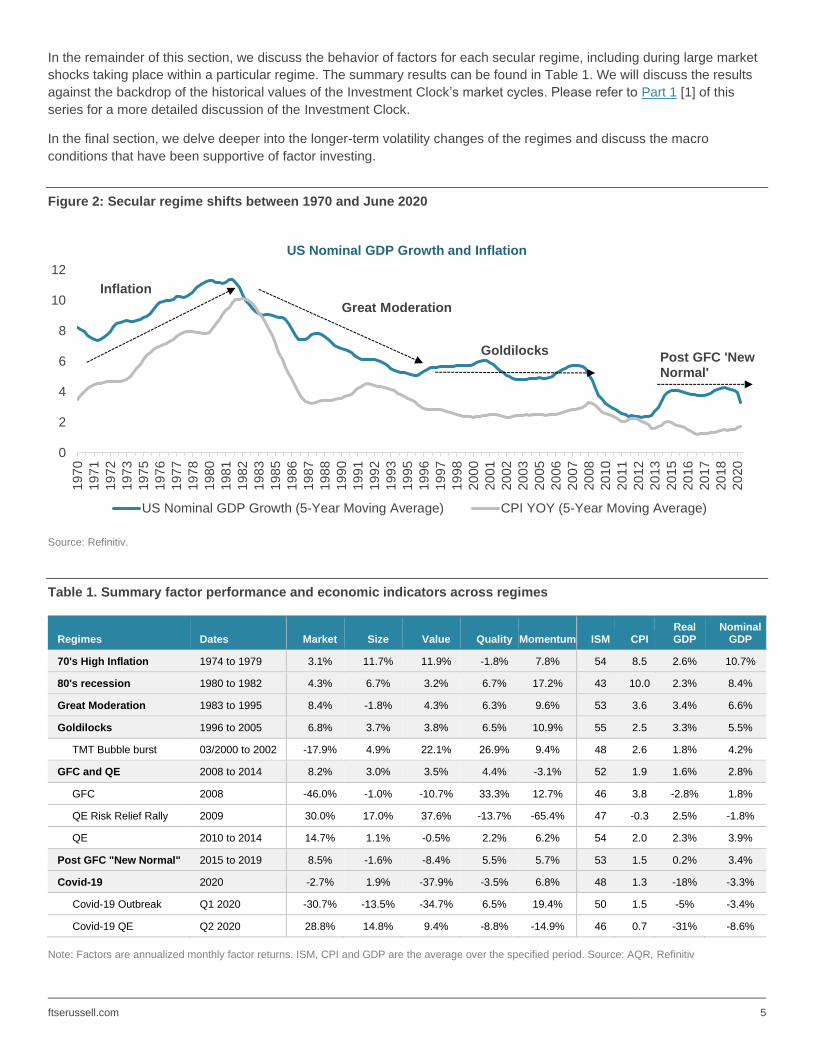
In the remainder of this section, we discuss the behavior of factors for each secular regime, including during large market
shocks taking place within a particular regime. The summary results can be found in Table 1. We will discuss the results
against the backdrop of the historical values of the Investment Clock’s market cycles. Please refer to Part 1 [1] of this
series for a more detailed discussion of the Investment Clock.
In the final section, we delve deeper into the longer-term volatility changes of the regimes and discuss the macro
conditions that have been supportive of factor investing.
Figure 2: Secular regime shifts between 1970 and June 2020
Source: Refinitiv.
Table 1. Summary factor performance and economic indicators across regimes
Regimes Dates Market Size Value Quality Momentum ISM CPI Real GDP
Nominal GDP
70's High Inflation 1974 to 1979 3.1% 11.7% 11.9% -1.8% 7.8% 54 8.5 2.6% 10.7%
80's recession 1980 to 1982 4.3% 6.7% 3.2% 6.7% 17.2% 43 10.0 2.3% 8.4%
Great Moderation 1983 to 1995 8.4% -1.8% 4.3% 6.3% 9.6% 53 3.6 3.4% 6.6%
Goldilocks 1996 to 2005 6.8% 3.7% 3.8% 6.5% 10.9% 55 2.5 3.3% 5.5%
TMT Bubble burst 03/2000 to 2002 -17.9% 4.9% 22.1% 26.9% 9.4% 48 2.6 1.8% 4.2%
GFC and QE 2008 to 2014 8.2% 3.0% 3.5% 4.4% -3.1% 52 1.9 1.6% 2.8%
GFC 2008 -46.0% -1.0% -10.7% 33.3% 12.7% 46 3.8 -2.8% 1.8%
QE Risk Relief Rally 2009 30.0% 17.0% 37.6% -13.7% -65.4% 47 -0.3 2.5% -1.8%
QE 2010 to 2014 14.7% 1.1% -0.5% 2.2% 6.2% 54 2.0 2.3% 3.9%
Post GFC "New Normal" 2015 to 2019 8.5% -1.6% -8.4% 5.5% 5.7% 53 1.5 0.2% 3.4%
Covid-19 2020 -2.7% 1.9% -37.9% -3.5% 6.8% 48 1.3 -18% -3.3%
Covid-19 Outbreak Q1 2020 -30.7% -13.5% -34.7% 6.5% 19.4% 50 1.5 -5% -3.4%
Covid-19 QE Q2 2020 28.8% 14.8% 9.4% -8.8% -14.9% 46 0.7 -31% -8.6%
Note: Factors are annualized monthly factor returns. ISM, CPI and GDP are the average over the specified period. Source: AQR, Refinitiv
0
2
4
6
8
10
12
19
70
19
71
19
72
19
73
19
75
19
76
19
77
19
78
19
80
19
81
19
82
19
83
19
85
19
86
19
87
19
88
19
90
19
91
19
92
19
93
19
95
19
96
19
97
19
98
20
00
20
01
20
02
20
03
20
05
20
06
20
07
20
08
20
10
20
11
20
12
20
13
20
15
20
16
20
17
20
18
20
20
US Nominal GDP Growth and Inflation
US Nominal GDP Growth (5-Year Moving Average) CPI YOY (5-Year Moving Average)
Great Moderation
Post GFC 'New Normal'
Goldilocks
Inflation

ftserussell.com 6
Regime 1: 1970s’ high inflation and early 1980s’ recession (1974 to 1982)
The 1970s were marked by double-digit inflation rates. At the root of the problem was the oil crisis and an accommodative
monetary policy financing a massive budget deficit. This led to a period of stagflation ‒ low growth with rapidly rising
prices. Professor Jeremy Siegel called the period the greatest failure of American macroeconomic policy in the post-war
period [6].
Inflation was quite volatile during that period. It first reached double digits in 1974, briefly calmed down around 1976,
before reaching an all-time high of 14% in the early 1980s. Under the leadership of Paul Volcker, the central bank
reversed its policies, raising interest rates to as high as 20% to get inflation under control, which was the onset of the
1980s recession. The graph below shows the historical economic cycles of the Investment Clock [1] and the cumulative
factor returns. It suggests that the 1970s are market by periods of slowdown and recovery, reaching bottom in the 1980s
recession period. A market recovery did not start until early 1983.
As the market initially fell in the early 1970s, Size had a bad run (-10%), whereas Value (8.1%) and Momentum (11%)
were the winning factor strategies. The onset of the recession in 1981 hurt Value (-20%) and benefited the long/short
Momentum factor (31%). In 1981, investors still traumatized by the erosion of money in the 1970s, started to buy cheap
quality stocks (Value (25%), Quality (7%)). Factor performance during the recession was marked by high and lows, but a
buy and hold strategy would have delivered a positive average annualized return across all factors.
Note: Economic cycles are the quarterly observations of the Investment Clock. Factors are the cumulative monthly returns. Source: FTSE Russell.
0
50
100
150
200
250
300
350
400
450
1970 1971 1972 1973 1974 1975 1976 1977 1978 1979 1980 1981 1982 1983
Montly C
um
ula
tive R
etu
rn
Economic Cycles and Factor PerformanceInflation & Recession: 1970 to January 1983
Slowdown
Contraction
Recovery
Expansion
size
value
quality
momentum
ftserussell.com 7
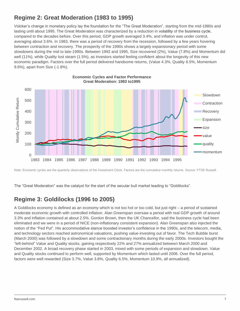
Regime 2: Great Moderation (1983 to 1995)
Volcker’s change in monetary policy lay the foundation for the “The Great Moderation”, starting from the mid-1980s and
lasting until about 1995. The Great Moderation was characterized by a reduction in volatility of the business cycle,
compared to the decades before. Over this period, GDP growth averaged 3.4%, and inflation was under control,
averaging about 3.6%. In 1983, there was a period of recovery from the recession, followed by a few years hovering
between contraction and recovery. The prosperity of the 1990s shows a largely expansionary period with some
slowdowns during the mid to late-1990s. Between 1992 and 1995, Size recovered (2%), Value (7.8%) and Momentum did
well (11%), while Quality lost steam (1.5%), as investors started feeling confident about the longevity of this new
economic paradigm. Factors over the full period delivered handsome returns, (Value 4.3%, Quality 6.5%, Momentum
9.6%), apart from Size (-1.8%).
Note: Economic cycles are the quarterly observations of the Investment Clock. Factors are the cumulative monthly returns. Source: FTSE Russell.
The “Great Moderation” was the catalyst for the start of the secular bull market leading to “Goldilocks”.
Regime 3: Goldilocks (1996 to 2005)
A Goldilocks economy is defined as an economy which is not too hot or too cold, but just right ‒ a period of sustained
moderate economic growth with controlled inflation. Alan Greenspan oversaw a period with real GDP growth of around
3.3% and inflation contained at about 2.5%. Gordon Brown, then the UK Chancellor, said the business cycle had been
eliminated and we were in a period of NICE (non-inflationary consistent expansion). Alan Greenspan also injected the
notion of the “Fed Put”. His accommodative stance boosted investor’s confidence in the 1990s, and the telecom, media,
and technology sectors reached astronomical valuations, pushing value-investing out of favor. The Tech Bubble burst
(March 2000) was followed by a slowdown and some contractionary months during the early 2000s. Investors bought the
“left-behind” Value and Quality stocks, gaining respectively 22% and 27% annualized between March 2000 and
December 2002. A broad recovery phase started in 2003, mixed with some periods of expansion and slowdown. Value
and Quality stocks continued to perform well, supported by Momentum which lasted until 2006. Over the full period,
factors were well rewarded (Size 3.7%, Value 3.8%, Quality 6.5%, Momentum 10.9%, all annualized).
0
100
200
300
400
500
600
1983 1984 1985 1986 1987 1988 1989 1990 1991 1992 1993 1994 1995
Montly C
um
ula
tive R
etu
rn
Economic Cycles and Factor PerformanceGreat Moderation: 1983 to1995
Slowdown
Contraction
Recovery
Expansion
size
value
quality
momentum

ftserussell.com 8
Note: Economic cycles are the quarterly observations of the Investment Clock. Factors are the cumulative monthly returns. Source: FTSE Russell.
Regime 4: Global Financial Crisis and quantitative easing (2007 to 2014)
Ben Bernanke, chairman of the Fed from 2006 to 2014, started his tenure worried about inflation risk. He oversaw 17
consecutive rate hikes and a Fed funds rate as high as 5.25% in June 2006, resulting in an inverted yield curve. This was
damaging to Value and Size strategies and investors sought the safety of Quality stocks. A period of slowdown begins at
the end of 2007, gliding into a contraction in response to the GFC. In 2008, the market almost halved (-46%), as investors
shunned cyclical Value stocks (-10.7%) and opted for the safe haven of Quality (33.3%), while Momentum (12.7%) held
up. Real GDP fell to -4.1% and inflation hit a low of -0.2%. In response to the first quantitative easing program in 2009,
there was a risk relief rally. Investors rotated out of Quality (-13.7%) into Small Cap (17%) Value (38%) strategies.
Momentum, being short high beta after the crisis, was caught out (-65%). Further quantitative easing between 2010 and
2014, stimulated the market (+14.7%), while hurting factor performance relative to prior regimes (Size 1.1%, Value -0.5%,
Quality 2.2%, Momentum 6.2%).
Note: Economic cycles are the quarterly observations of the Investment Clock. Factors are the cumulative monthly returns. Source: FTSE Russell.
0
20
40
60
80
100
120
140
160
180
2006 2007 2008 2009 2010 2011 2012 2013
Montly C
um
ula
tive R
etu
rnEconomic Cycles and Factor Performance
Goldilocks: 1996 to 2006
Slowdown
Contraction
Recovery
Expansion
size
value
quality
momentum
0
20
40
60
80
100
120
140
160
180
2014 2015 2016 2017 2018 2019 2020
Montly C
um
ula
tive R
etu
rn
Economic Cycles and Factor PerformanceGFC: 2007 to 2014
Slowdown
Contraction
Recovery
Expansion
size
value
quality
momentum

ftserussell.com 9
Regime 5: Normalization: unwinding quantitative easing and Covid-19 (2015 to 2020)
Over the past decade, all-time low Fed rates and an expanding balance sheet have stimulated the economy to move
between expansion and slowdown, but volatility spikes and market stress have also resulted in periods of contraction and
recovery. The chairman of the Fed, Janet Yellen, and then Jerome Powell, set out the task of a gradual unwinding of the
Federal Reserve’s $4.5 trillion balance sheet that had swelled during the previous decade, as it engaged in QE in
response to the GFC. Now that the economy had recovered, with real GDP at 2.49% and inflation at 1.55%, the Fed had
planned to shrink it again. Investors became nervous about the unwinding process and continued their preference for high
Momentum (5.5%) Quality (6.44%) stocks, shunning Value (-5.4%) and Size (-1.9%). This was also the period US
technology stocks (FAANG) took off. An economic expansion started off 2020, but Covid-19 led to the largest contraction
since the 1970s. In Q1 2020, the market dropped -30.6% and Value took the market by surprise, falling -37.9%, whereas
Quality (6%) and Momentum (6.8%) held course. The Fed moved away from normalization and back to an extremely
accommodative monetary policy, with the Fed’s balance sheet almost doubling in the second quarter of 2020. This gave
rise to a market recovery in June. In Q2 2020, the Market (28.8%), Size (15%) and Value (9%) did well, while Quality
(-9%) and Momentum (-15%) lost some ground. Real GDP (-31%) is at an all-time low and inflation has fallen further
below the 2% target, to 0.70%.
Note: Economic cycles are the quarterly observations of the Investment Clock. Factors are the cumulative monthly returns. Source FTSE Russell.
To conclude, the Investment Clock’s limitation is the assumption of a normalized or constant cycle. We have seen that the
notion of the cycle has changed radically over time. The new thinking focuses on regimes. Regimes have a significant
impact on factor payoffs, driven by changes in the magnitude and volatility of economic indicators. In the final section, we
focus on the impact of quantitative easing on the post-GFC factor performance against the context of previous regimes.
0
20
40
60
80
100
120
140
160
180
2014 2015 2016 2017 2018 2019 2020
Montly C
um
ula
tive R
etu
rn
Economic Cycles and Cumulative Factor Performance'QE Normalization' & Covid-19: 2015 to June 2020
Slowdown
Contraction
Recovery
Expansion
size
value
quality
momentum

ftserussell.com 10
2. Key question: how has quantitative easing impacted factor performance? Since 2009, markets have been stimulated by the Fed’s massive quantitative easing program, which has led to a
significant reduction in the volatility of the business cycle. In this section, we examine the period from 1970 to June 2020,
and identify three major shifts in the volatility of the economic cycle (Table 2):
1. the High Volatility Regime of the 1970s inflation boom and 1980s recession bust;
2. the Moderate Volatility Regime of the Great Moderation and continued into Goldilocks;
3. the Low Volatility Regime of 12 years of stagnation since the GFC.
We will link factor performance to these economic volatility regimes and document distinctive behavior as a guide to future
expectations. Then, we will discuss the levels and volatility of real GDP growth and inflation rates, to establish the
framework. This will be followed with a discussion of the performance and risk characteristics of factors across the
economic volatility regimes.
Table 2: Economic cycle volatility and long-term regimes
Dates Economic Cycle Volatility Regimes Covered
1970-1982 High High Inflation & Recession
1983-2005 Moderate Great Moderation and Goldilocks
2010-2020 Low QE and New Normal
1. Economic Volatility Regimes and Economic Indicators
To establish the distinctive nature of the economic volatility regimes, we first examine the level and volatility of inflation
and real GDP (Figure 3). Inflation reached an all-time high (14.6%) in the 1970s and an all time-low (-0.2%) post-GFC (till
June 2020). The general trend across regimes is downward: inflation averaged 7.8% during the High Volatility Regime,
3.6% in the Moderate period and has fallen to 1.7% during the Low Volatility Regime, post-GFC period. Despite massive
economic stimulus, inflation has remained below its 2% target since 2009.
During the High phase, GDP recovered to an average of 2.6%, but was quite volatile, ranging between -2.6% and 7.6%.
The Moderate phase was marked by a healthy economic growth of around 3.5%. Real GDP growth hit an all-time low
(-31.4%) in response to Covid-19, reducing real GDP growth post-GFC to a 1.4% low.
It is clear both the level and volatility of the economic indicators have substantially narrowed since the GFC. The impact of
QE has led to a significant reduction in the volatility of the business cycle, with one big outlier due to Covid-19.

ftserussell.com 11
Figure 3. Economic growth and inflation across volatility regimes
Note: CPI is quarterly YOY change, GDP is quarterly YoY change in Real GDP. Source: Refinitiv.
2. Economic Volatility Regime: Factor Performance
We discussed earlier how QE has stimulated the market despite below trend economic growth and inflation expectations.
Table 3 shows a steady upward trend in the annualized market return: 2.1% in the High to 11.5% in the Low regime. Even
on a risk-adjusted basis, the market return post-GFC is superior. How has this impacted factor returns on an absolute and
risk-adjusted basis? Size has not performed since the High period. Value’s best performance was during the High (8.7%),
followed by the Moderate phase (4.3%), but lost money post GFC (-4.6%). The results are confirmed on a risk-adjusted
basis. Even though Quality and Momentum had a good run post-GFC, on a risk-adjusted basis, the Moderate Volatility
Regime was superior. The equally weighted portfolio is a weighted average of the four factors. It is noticeable how the
annualized return and risk-adjusted returns have diminished over time. In the Low phase, diversification across factors
delivered a mere 1.2% per annum, leading to a low 0.13 on a risk-adjusted return basis. This is the only period where only
two out of four factors delivered on a buy-and-hold basis.
Table 3. Factor absolute and risk-adjusted returns: High, Moderate, Low Volatility regimes
Factors Average Annualized Return Risk-Adjusted Return
HIGH MODERATE LOW HIGH MODERATE LOW
Market 2.1% 8.6% 11.5% 0.1 0.6 0.8
Size 3.9% -1.6% -0.3% 0.3 -0.2 0.0
Value 8.7% 4.3% -4.6% 0.7 0.5 -0.4
Quality 2.1% 6.0% 4.0% 0.3 1.1 0.5
Momentum 11.0% 9.4% 5.9% 0.8 1.0 0.5
EW 4 Factors 6.4% 4.6% 1.2% 0.55 0.60 0.13
Note: Annualized monthly factor returns across volatility regimes. Risk-adjusted returns equal annualized returns divided by annualized standard deviation. The EW 4-factor portfolio, equally weights Size, Value, Quality and Momentum. Source: AQR.
7.8
2.9
14.6
3.6
1.2
6.4
1.7
-0.2
3.8
-2.0
0.0
2.0
4.0
6.0
8.0
10.0
12.0
14.0
16.0
CPI Average CPI Low CPI High
1. High 1. Moderate 4. Post GFC Low
2.6%
-2.6%
7.6%
3.5%
-1.4%
8.6%
1.4%
-31.4%
3.3%
-35.0%
-30.0%
-25.0%
-20.0%
-15.0%
-10.0%
-5.0%
0.0%
5.0%
10.0%
GDP Average GDP Low GDP High
1. High 1. Moderate 4. Post GFC Low
ftserussell.com 12
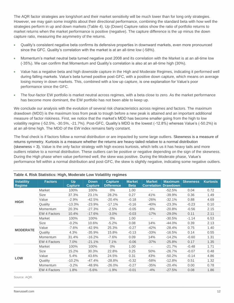
The AQR factor strategies are long/short and their market sensitivity will be much lower than for long only strategies.
However, we may gain some insights about their directional performance, combining the standard beta with how well the
strategies perform in up and down markets (Table 4). Up (Down) Capture ratios show the ratio of portfolio returns to
market returns when the market performance is positive (negative). The capture difference is the up minus the down
capture ratio, measuring the asymmetry of the returns.
• Quality’s consistent negative beta confirms its defensive properties in downward markets, even more pronounced
since the GFC. Quality’s correlation with the market is at an all-time low (-58%).
• Momentum’s market neutral beta turned negative post 2008 and its correlation with the Market is at an all-time low
(-35%). We can confirm that Momentum and Quality’s correlation is also at an all-time high (30%).
• Value has a negative beta and high downside capture in the High and Moderate Regimes, indicating it performed well
during falling markets. Value’s beta turned positive post-GFC, with a positive down capture, which means on average
losing money in down markets. This, combined with a low up capture, is one explanation for Value’s poor
performance since the GFC.
• The four-factor EW portfolio is market neutral across regimes, with a beta close to zero. As the market performance
has become more dominant, the EW portfolio has not been able to keep up.
We conclude our analysis with the evolution of several risk characteristics across regimes and factors. The maximum
drawdown (MDD) is the maximum loss from peak to trough before a new peak is attained and an important additional
measure of factor riskiness. First, we notice that the market’s MDD has become smaller going from the high to low
volatility regime (-52.5%, -30.5%, -21.7%). Post-GFC, Quality’s MDD is the lowest (-12.8%) whereas Value’s (-50.2%) is
at an all-time high. The MDD of the EW index remains fairly constant.
The final check is if factors follow a normal distribution or are impacted by some large outliers. Skewness is a measure of
returns symmetry. Kurtosis is a measure whether the returns are heavy-tailed relative to a normal distribution
(skewness = 3). Value is the only factor strategy with high excess kurtosis, which tells us it has heavy tails and more
outliers relative to a normal distribution. These outliers can be positive or negative depending on the sign of the skewness.
During the High phase when value performed well, the skew was positive. During the Moderate phase, Value’s
performance fell within a normal distribution and post-GFC, the skew is slightly negative, indicating some negative outliers.
Table 4. Risk Statistics: High, Moderate Low Volatility regimes
Volatility Regime
Factors Up Capture
Down Capture
Capture Difference
Market Beta
Market Correlation
Maximum Drawdown
Skewness Kurtosis
HIGH
Market 100% 100% 0% 1.00 - -52.5% 0.04 0.72
Size 37.3% 23.1% 28.2% 0.27 41% -39.9% 0.36 1.49
Value -2.9% -42.5% -20.4% -0.18 -26% -32.1% 0.88 4.69
Quality -13.3% -23.9% -17.1% -0.16 -40% -23.3% -0.23 0.10
Momentum 20.3% -27.3% -2.5% -0.05 -6% -20.8% -0.56 2.15
EW 4 Factors 10.4% -17.6% -3.0% -0.03 -17% -29.0% 0.11 2.11
MODERATE
Market 100% 100% 0% 1.00 - -30.5% -1.14 6.53
Size -0.2% 10.6% -5.2% 0.08 14% -44.0% 0.39 2.13
Value -7.6% -42.9% 25.3% -0.27 -42% -28.4% 0.75 1.40
Quality 4.3% -35.9% 15.8% -0.13 -33% -16.5% 0.14 0.55
Momentum 31.4% -16.2% -7.6% 0.09 14% -14.2% -0.60 1.31
EW 4 Factors 7.0% -21.1% 7.1% -0.06 -37% -25.8% 0.17 1.35
LOW
Market 100% 100% 0% 1.00 - -21.7% -0.48 1.71
Size 15.2% 30.3% 22.8% 0.25 50% -26.7% -0.07 0.48
Value 5.4% 43.6% 24.5% 0.31 43% -50.2% -0.14 4.86
Quality -10.2% -47.4% -28.8% -0.32 -58% -12.8% 0.51 1.32
Momentum -3.2% -48.9% -26.0% -0.27 -35% -20.4% 0.00 0.78
EW 4 Factors 1.8% -5.6% -1.9% -0.01 -4% -27.5% 0.08 1.86
Source: AQR.
ftserussell.com 13
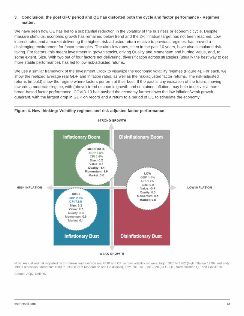
3. Conclusion: the post GFC period and QE has distorted both the cycle and factor performance - Regimes
matter.
We have seen how QE has led to a substantial reduction in the volatility of the business or economic cycle. Despite
massive stimulus, economic growth has remained below trend and the 2% inflation target has not been reached. Low
interest rates and a market delivering the highest risk-adjusted return relative to previous regimes, has proved a
challenging environment for factor strategies. The ultra-low rates, seen in the past 10 years, have also stimulated risk-
taking. For factors, this meant investment in growth stocks, driving Quality and Momentum and hurting Value, and, to
some extent, Size. With two out of four factors not delivering, diversification across strategies (usually the best way to get
more stable performance), has led to low risk-adjusted returns.
We use a similar framework of the Investment Clock to visualize the economic volatility regimes (Figure 4). For each, we
show the realized average real GDP and inflation rates, as well as the risk-adjusted factor returns. The risk-adjusted
returns (in bold) show the regime where factors perform at their best. If the past is any indication of the future, moving
towards a moderate regime, with (above) trend economic growth and contained inflation, may help to deliver a more
broad-based factor performance. COVID-19 has pushed the economy further down the low inflation/weak growth
quadrant, with the largest drop in GDP on record and a return to a period of QE to stimulate the economy.
Figure 4. New thinking: Volatility regimes and risk-adjusted factor performance
Note: Annualized risk-adjusted factor returns and average real GDP and CPI across volatility regimes. High: 1970 to 1982 (high inflation 1970s and early 1980s recession. Moderate: 1983 to 1985 (Great Moderation and Goldilocks), Low: 2010 to June 2020 (GFC, QE, Normalization QE and Covid-19).
Source: AQR, Refinitiv.
ftserussell.com 14
3. Summary and conclusions In Part one of this series, “The Investment Clock: linking factor behavior to the economic cycle,” [1] we used the
Investment Clock framework to understand how factors respond to its economic cycles. The findings are intuitive, but
post-GFC, we observe more return volatility and lower average factor payoffs.
The Investment Clock is based on the assumption of a normalized economic pattern. Its existence is questionable,
especially post-GFC, due to the massive quantitative easing implemented to prop up the global economy. An evolution of
the Investment Clock is to observe a pattern of secular regime shifts. Secular regimes are found to have a significant
impact on factor payoffs, driven by changes in the magnitude and volatility of economic indicators. Historically factors
have done well during regimes with trend economic growth and target but contained inflation like the Great Moderation
and Goldilocks.
To get a better understanding of the impact of quantitative easing on factor performance, we define economic volatility
regimes, based on the level and volatility of inflation and real GDP. We identify three major shifts in economic volatility
between 1957 and 2020:
1. High volatility of the hyper-inflation seventies and early 80s recession;
2. Moderate volatility of the great moderation and goldilocks;
3. Low volatility since the GFC.
Average inflation has fallen going from the High to the Low economic volatility regime, whereas average real GDP growth
was the highest during the period of moderate economic volatility.
We find that QE and the ultra-low interest rates have stimulated risk taking favoring high duration growth stocks. This has
led to a surge in Quality and Momentum, leaving Value and Size behind, resulting in poor performance of a diversified
(equal weighted) four-factor portfolio. If the past is any indication of the future, a more moderate regime, with trend
economic growth and target inflation, is a positive economic climate for broad based and diversified factor investing.

ftserussell.com 15
References [1] van Boven, M., Do factors carry information about the cycle? Part 1, The Investment Clock: linking factor behavior to
the economic cycle”, FTSE Russell, 2020.
[2] Ferson, W.E., Harvey C.R., “The Variation of Economic Risk Premiums,” Journal of Political Economy, (1991), pp.
385–415.
[3] Fama, E.F., French, K.R., 1993. Common risk factors in the returns on stocks and bonds. Journal of Financial
Economics 33, 3–56.
[4] Vassalou, M., Can Book-to-Market, Size and Momentum be Risk Factors that Predict Economic Growth? (1999), draft
version.
[5] Aretz K., Bartram S.M., Pope P., Macro-economic Risk and Factor Based Portfolios, Journal of Banking & Finance 34
(2010), 1383-1399.
[6] Siegel,J., Stocks for the Long Run: A Guide for Long-Term Growth, 1994.

ftserussell.com 16
Appendix
Table 1: Data definitions
Factor Definitions AQR Long/Short Factors
Factors AQR Name Data input
Market Market Value-weighted return on all available stocks minus one-month treasury bills
Size SMB Total Market Value Equity (ME)
Value HML Devil Book Equity/ME
Quality Quality minus Junk Measures of Profitability: Growth, Safety and Payout
Momentum Momentum 12-month prior return, skipping the most recent month
Data Source: www.aqr.com, monthly data files
Macro-economic Data
Macro Data Definition Data Frequency
GDP Year-on-Year quarterly US GDP rate Annual
Inflation Year on Year CPI, quarterly and monthly Annual and Monthly
ISM ISM, monthly Monthly
Source: Refinitiv.

ftserussell.com 17
About FTSE Russell
FTSE Russell is a leading global provider of benchmarks, analytics and data solutions with multi-asset capabilities,
offering a precise view of the markets relevant to any investment process. For over 30 years, leading asset owners,
asset managers, ETF providers and investment banks have chosen FTSE Russell indexes to benchmark their
investment performance and create investment funds, ETFs, structured products and index-based derivatives. FTSE
Russell indexes also provide clients with tools for performance benchmarking, asset allocation, investment strategy
analysis and risk management.
To learn more, visit ftserussell.com; email [email protected]; or call your regional Client Service Team office
EMEA
+44 (0) 20 7866 1810
North America
+1 877 503 6437
Asia-Pacific
Hong Kong +852 2164 3333
Tokyo +81 3 4563 6346
Sydney +61 (0) 2 8823 3521
© 2020 London Stock Exchange Group plc and its applicable group undertakings (the “LSE Group”). The LSE Group includes (1) FTSE International Limited (“FTSE”), (2) Frank Russell Company (“Russell”), (3) FTSE Global Debt Capital Markets Inc. and FTSE Global Debt Capital Markets Limited (together, “FTSE Canada”), (4) MTSNext Limited (“MTSNext”), (5) Mergent, Inc. (“Mergent”), (6) FTSE Fixed Income LLC (“FTSE FI”), (7) The Yield Book Inc (“YB”) and (8) Beyond Ratings S.A.S. (“BR”). All rights reserved.
FTSE Russell® is a trading name of FTSE, Russell, FTSE Canada, MTSNext, Mergent, FTSE FI, YB and BR. “FTSE®”, “Russell®”, “FTSE Russell®”, “MTS®”, “FTSE4Good®”, “ICB®”, “Mergent®”, “The Yield Book®”, “Beyond Ratings®“ and all other trademarks and service marks used herein (whether registered or unregistered) are trademarks and/or service marks owned or licensed by the applicable member of the LSE Group or their respective licensors and are owned, or used under licence, by FTSE, Russell, MTSNext, FTSE Canada, Mergent, FTSE FI, YB or BR. FTSE International Limited is authorised and regulated by the Financial Conduct Authority as a benchmark administrator.
All information is provided for information purposes only. All information and data contained in this publication is obtained by the LSE Group, from sources believed by it to be accurate and reliable. Because of the possibility of human and mechanical error as well as other factors, however, such information and data is provided “as is” without warranty of any kind. No member of the LSE Group nor their respective directors, officers, employees, partners or licensors make any claim, prediction, warranty or representation whatsoever, expressly or impliedly, either as to the accuracy, timeliness, completeness, merchantability of any information or of results to be obtained from the use of the FTSE Russell products, including but not limited to indexes, data and analytics or the fitness or suitability of the FTSE Russell products for any particular purpose to which they might be put. Any representation of historical data accessible through FTSE Russell products is provided for information purposes only and is not a reliable indicator of future performance.
No responsibility or liability can be accepted by any member of the LSE Group nor their respective directors, officers, employees, partners or licensors for (a) any loss or damage in whole or in part caused by, resulting from, or relating to any error (negligent or otherwise) or other circumstance involved in procuring, collecting, compiling, interpreting, analysing, editing, transcribing, transmitting, communicating or delivering any such information or data or from use of this document or links to this document or (b) any direct, indirect, special, consequential or incidental damages whatsoever, even if any member of the LSE Group is advised in advance of the possibility of such damages, resulting from the use of, or inability to use, such information.
No member of the LSE Group nor their respective directors, officers, employees, partners or licensors provide investment advice and nothing contained herein or accessible through FTSE Russell products, including statistical data and industry reports, should be taken as constituting financial or investment advice or a financial promotion.
Past performance is no guarantee of future results. Charts and graphs are provided for illustrative purposes only. Index returns shown may not represent the results of the actual trading of investable assets. Certain returns shown may reflect back-tested performance. All performance presented prior to the index inception date is back-tested performance. Back-tested performance is not actual performance, but is hypothetical. The back-test calculations are based on the same methodology that was in effect when the index was officially launched. However, back- tested data may reflect the application of the index methodology with the benefit of hindsight, and the historic calculations of an index may change from month to month based on revisions to the underlying economic data used in the calculation of the index.
This document may contain forward-looking assessments. These are based upon a number of assumptions concerning future conditions that ultimately may prove to be inaccurate. Such forward-looking assessments are subject to risks and uncertainties and may be affected by various factors that may cause actual results to differ materially. No member of the LSE Group nor their licensors assume any duty to and do not undertake to update forward-looking assessments.
No part of this information may be reproduced, stored in a retrieval system or transmitted in any form or by any means, electronic, mechanical, photocopying, recording or otherwise, without prior written permission of the applicable member of the LSE Group. Use and distribution of the LSE Group data requires a licence from FTSE, Russell, FTSE Canada, MTSNext, Mergent, FTSE FI, YB, BR and/or their respective licensors.