distributional lexical semantics ii: getting into the...
TRANSCRIPT
Distributional Lexical Semantics II:Getting into the details
Marco Baroni
UPF Computational Semantics Course

Outline
Building the model
Weighting dimensions
Cosine similarity
Dimensionality reductionSingular Value DecompositionRandom Indexing

Corpus pre-processing
I Minimally, corpus must be tokenizedI POS tagging, lemmatization, dependency parsing. . .I Trade-off between deeper linguistic analysis and
I need for language-specific resourcesI possible errors introduced at each stage of the analysisI more parameters to tune

Contexts and dimensions
I One fundamental difference:I Non-lexical aspects of contexts as filtersI Non-lexical aspects of contexts as links

Window-based
The dog barks in the alley.
I Context as filter (e.g., Rapp 2003):dog bark; bark dog; bark alley; alley bark
I Context as link (e.g., HAL):dog bark-r; bark dog-l; bark alley-r; alley bark-l

Dependency-based
The dog barks in the alley.
I Context as filter (e.g., Padó & Lapata):dog bark; bark dog
I Context as link (e.g., Grefenstette 1994, Lin 1998, Curran& Moens 2002):dog bark-subj−1; bark dog-subj

Filters vs. links
I With filters, data less sparse (man kills and kills man bothmap to a kill dimension of the man vector)
I With linksI more sensitivity to semantic distinctions (kill-subj−1 and
kill-obj−1 are rather different things!)I links provide a form of “typing” of dimensions (the “subject”
dimensions, the “for” dimensions, etc.)I we will see importance of this when we discuss relational
similarity

Outline
Building the model
Weighting dimensions
Cosine similarity
Dimensionality reductionSingular Value DecompositionRandom Indexing

Dimension weightingThe basic intuition
word1 word2 freq 1 2 freq 1 freq 2dog small 855 33,338 490,580dog domesticated 29 33,338 918

Mutual InformationChurch & Hanks (1990)
MI(w1, w2) = log2Pcorpus(w1, w2)
Pind(w1, w2)
MI(w1, w2) = log2Pcorpus(w1, w2)
Pcorpus(w1)Pcorpus(w2)
P(w1, w2) =fq(w1, w2)
N
P(w) =fq(w)
N

Mutual Information
I MI estimation (ignoring the logarithm):
P(w1, w2)
P(w1)P(w2)=
fq(w1,w2)N
fq(w1)N
fq(w2)N
=
fq(w1, w2)
N× N2
fq(w1)fq(w2)=
fq(w1, w2)Nfq(w1)fq(w2)
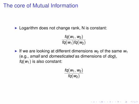
The core of Mutual Information
I Logarithm does not change rank, N is constant:
fq(w1, w2)
fq(w1)fq(w2)
I If we are looking at different dimensions w2 of the same w1(e.g., small and domesticated as dimensions of dog),fq(w1) is also constant:
fq(w1, w2)
fq(w2)

Mutual Information core
word1 word2 freq 1 2 freq 2 MI coredog small 855 490,580 0.00174dog domesticated 29 918 0.03159
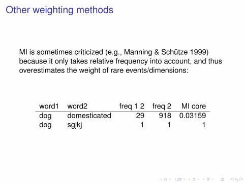
Other weighting methods
MI is sometimes criticized (e.g., Manning & Schütze 1999)because it only takes relative frequency into account, and thusoverestimates the weight of rare events/dimensions:
word1 word2 freq 1 2 freq 2 MI coredog domesticated 29 918 0.03159dog sgjkj 1 1 1
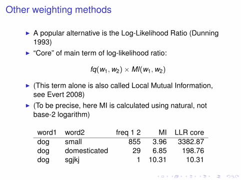
Other weighting methods
I A popular alternative is the Log-Likelihood Ratio (Dunning1993)
I “Core” of main term of log-likelihood ratio:
fq(w1, w2)×MI(w1, w2)
I (This term alone is also called Local Mutual Information,see Evert 2008)
I (To be precise, here MI is calculated using natural, notbase-2 logarithm)
word1 word2 freq 1 2 MI LLR coredog small 855 3.96 3382.87dog domesticated 29 6.85 198.76dog sgjkj 1 10.31 10.31

Weighting methods
I Many, many alternative weighting methods (Evert 2005,2008)
I In my experience (see also Schone & Jurafsky 2001), bigdivide is between MI-like measures, that do not have anabsolute co-occurrence frequency term, and LLR-likemeasures, that do
I Unfortunately, attempts to determine the best weightingmethod are inconclusive

Many many parameters
I How many dimensions, and which?I Stop words?I Window-based weighting?I How do you transform raw frequencies?I Do you perform dimensionality reduction?I Etc.I See Bullinaria & Levy 2007, Bullinaria 2008 for a
systematic exploration of some of these parameters
Outline
Building the model
Weighting dimensions
Cosine similarity
Dimensionality reductionSingular Value DecompositionRandom Indexing

Contexts as vectors
runs legsdog 1 4cat 1 5car 4 0

Semantic space
0 1 2 3 4 5 6
01
23
45
6
runs
legs
car (4,0)
dog (1,4)
cat (1,5)

Semantic similarity as angle between vectors
0 1 2 3 4 5 6
01
23
45
6
runs
legs
car (4,0)
dog (1,4)
cat (1,5)

Measuring angles by computing cosines
I Cosine is most common similarity measure in distributionalsemantics, and the most sensible one from a geometricalpoint of view
I Ranges from 1 for parallel vectors (perfectly correlatedwords) to 0 for orthogonal (perpendicular) words/vectors
I It goes to -1 for parallel vectors pointing in oppositedirections (perfectly inversely correlated words), as long asweighted co-occurrence matrix has negative values
I (Angle is obtained from cosine by applying the arc-cosinefunction, but it is rarely used in computational linguistics)
Trigonometry review
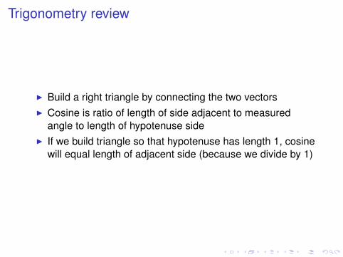
I Build a right triangle by connecting the two vectorsI Cosine is ratio of length of side adjacent to measured
angle to length of hypotenuse sideI If we build triangle so that hypotenuse has length 1, cosine
will equal length of adjacent side (because we divide by 1)

Cosine
0.0 0.2 0.4 0.6 0.8 1.0
0.0
0.2
0.4
0.6
0.8
1.0
x
y
θθ
0.0 0.2 0.4 0.6 0.8 1.00.
00.
20.
40.
60.
81.
0
x
yθθ

Computing the cosine
I Given a and b, two vectors (segments from the origin) oflength 1 and with n dimensions, cosine is given by:
i=n∑i=1
ai × bi

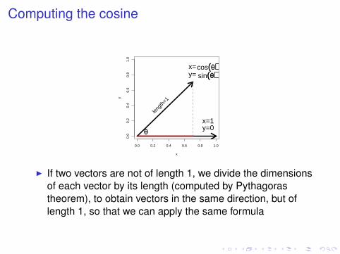
Computing the cosine
I For simplicity, consider a two-dimensional space (theclassic “two-coordinates” space), where a has 0-value onthe second dimension (i.e., it is parallel to the x-axis)
I Then, the a coordinates are 1 and 0; the b coordinates arecos(θ) and sin(θ):
0.0 0.2 0.4 0.6 0.8 1.0
0.0
0.2
0.4
0.6
0.8
1.0
x
y
θθ
x=cos((θθ))y= sin((θθ))
x=1y=0
lengt
h=1

Computing the cosine
0.0 0.2 0.4 0.6 0.8 1.00.
00.
20.
40.
60.
81.
0x
y
θθ
x=cos((θθ))y= sin((θθ))
x=1y=0
lengt
h=1
I If we apply the formula:i=n∑i=1
ai × bi
we get:
(1× cos(θ)) + (0× sin(θ)) = cos(θ)
i.e., the cosine between the two vectors

Computing the cosine
0.0 0.2 0.4 0.6 0.8 1.0
0.0
0.2
0.4
0.6
0.8
1.0
x
y
θθ
x=cos((θθ))y= sin((θθ))
x=1y=0
lengt
h=1
I With a bit of trigonometry, this generalizes to any length-1vector pair
I Geometric intuition: we can always rotate the vectors bysame amount so that one is parallel to x-axis, withoutchanging the angle size
Computing the cosine
0.0 0.2 0.4 0.6 0.8 1.0
0.0
0.2
0.4
0.6
0.8
1.0
x
y
θθ
x=cos((θθ))y= sin((θθ))
x=1y=0
lengt
h=1
I If two vectors are not of length 1, we divide the dimensionsof each vector by its length (computed by Pythagorastheorem), to obtain vectors in the same direction, but oflength 1, so that we can apply the same formula

Computing the cosine
0.0 0.2 0.4 0.6 0.8 1.00.
00.
20.
40.
60.
81.
0
x
y
θθ
x=cos((θθ))y= sin((θθ))
x=1y=0
lengt
h=1
I Putting the two steps together (normalization to length 1and cosine computation for vectors of length 1) we obtainthe general formula to compute the cosine:∑i=n
i=1 ai × bi√∑i=ni=1 a2 ×
√∑i=ni=1 b2
I This generalizes to any n!

Computing the cosineExample
∑i=ni=1 ai × bi√∑i=n
i=1 a2 ×√∑i=n
i=1 b2
runs legsdog 1 4cat 1 5car 4 0
cosine(dog,cat) = (1×1)+(4×5)√12+42×
√12+52
= 0.9988681
arc-cosine(0.9988681) = 2.72 degrees
cosine(dog,car) = (1×4)+(4×0)√12+42×
√42+02
= 0.2425356
arc-cosine(0.2425356) = 75.85 degrees

Computing the cosineExample
0 1 2 3 4 5 6
01
23
45
6
runs
legs
car (4,0)
dog (1,4)
cat (1,5)
75.85 degrees
2.72 degrees
Cosine intuition
I When computing the cosine, the values that two vectorshave for the same dimensions (coordinates) are multiplied
I Two vectors/words will have a high cosine if they tend tohave high values for the same dimensions/contexts
I If we center the vectors so that their mean value is 0, thecosine of the centered vectors is the same as the Pearsoncorrelation coefficient
I If, as it is often the case in computational linguistics, wehave only positive scores, and we do not center thevectors, then the cosine can only take positive values, andthere is no “canceling out” effect
I As a consequence, cosines tend to be very high, muchhigher than the corresponding correlation coefficients

Other measures and the kernel trick
I Cosines are well-defined, well understood way to measuresimilarity in a vector space
I Other measures based on other, often non-geometricprinciples (Lin’s information theoretic measure,Kullback/Leibler divergence. . . ) bring us outside the scopeof vector spaces, and their application to semantic vectorscan be iffy and ad-hoc
I Stefan Evert’s advice:I Tweak your space, don’t tweak the similarity measure!I Map data to higher dimensionality space, and compute
cosine thereI Some functions applied to two vectors give a result that is
equivalent to computing the cosine in a higherdimensionality space, without requiring explicit computation(the “kernel trick”)

Outline
Building the model
Weighting dimensions
Cosine similarity
Dimensionality reductionSingular Value DecompositionRandom Indexing

Dimensionality reduction
I Distributional semantics recap:I Collect co-occurrence counts for target words and corpus
contextsI (Optionally transform the raw counts into some other score)I Build the target-word-by-context matrix, with each word
represented by the vector of values it takes on eachcontextual dimension
I Dimensionality reduction:I Reduce the target-word-by-context matrix to a lower
dimensionality matrix (a matrix with less – linearlyindependent – columns/dimensions)
I Two main reasons:I Smoothing: capture “latent dimensions” that generalize
over sparser surface dimensions (SVD)I Efficiency/space: sometimes the matrix is so large that you
don’t even want to construct it explicitly (Random Indexing)

Outline
Building the model
Weighting dimensions
Cosine similarity
Dimensionality reductionSingular Value DecompositionRandom Indexing

Singular Value Decomposition
I General technique from Linear Algebra (essentially, thesame as Principal Component Analysis, PCA)
I Given a matrix (e.g., a word-by-context matrix) of m × ndimensionality, construct a m × k matrix, where k << n(and k < m)
I E.g., from a 20,000 words by 10,000 contexts matrix to a20,000 words by 300 “latent dimensions” matrix
I k is typically an arbitrary choiceI From linear algebra, we know that and how we can find the
reduced m × k matrix with orthogonal dimensions/columnsthat preserves most of the variance in the original matrix
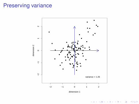
Preserving variance
−2 −1 0 1 2
−2
−1
01
2
dimension 1
dim
ensi
on 2
●
●
●
●
●
●
●
●
●
●●
●
●●
●
●
●
●
●
●
●
●
●
●
●
●
●
●
●
●
●
●
●●
●
●
●
●
●
●
●●
●
●
●
●
●
●
●
●
●
●
●
●
●
●●
●
●
●
●
●
● ●
●
●
●
●●
●
●
●
●
●
●
●
●
● ●
●
●
●
●
●
●
●
●
●
●
●
●
●
●●
●
●
●
●
●
●
●
●
●
●
●
●
●
●
●
●
●
variance = 1.26

Preserving variance
−2 −1 0 1 2
−2
−1
01
2
dimension 1
dim
ensi
on 2
●
●
●
●
●
●
●
●
●
●●
●
●●
●
●
●
●
●
●
●
●
●
●
●
●
●
●
●
●
●
●
●●
●
●
●
●
●
●
●●
●
●
●
●
●
●
●
●
●
●
●
●
●
●●
●
●
●
●
●
● ●
●
●
●
●●
●
●
●
●
●
●
●
●
● ●
●
●
●
●
●
●
●
●
●
●
●
●
●
●●
●
●
●
●
●
●
●
●
●
●
●
●
●
●
●
●
●

Preserving variance
−2 −1 0 1 2
−2
−1
01
2
dimension 1
dim
ensi
on 2
●
●
●
●
●
●
●
●
●
●●
●
●●
●
●
●
●
●
●
●
●
●
●
●
●
●
●
●
●
●
●
●●
●
●
●
●
●
●
●●
●
●
●
●
●
●
●
●
●
●
●
●
●
●●
●
●
●
●
●
● ●
●
●
●
●●
●
●
●
●
●
●
●
●
● ●
●
●
●
●
●
●
●
●
●
●
●
●
●
●●
●
●
●
●
●
●
●
●
●
●
●
●
●
●
●
●
●
●
●
●
●
●
●
●
●
●●
●
●●●
●
●
●
●
●
●
●
●
●
●
●
●
●
●
●
●
●
●
●
●
●
●
●
●
●
●
●●●
●●
●
●
●
●
●
●
●
●
●
●
●
●
●
●●
●
●
●
●
●
●
●
●
●
●
●●
●
●
●●
●
●
●
●
●
●
●
●
●
●
●
●
●
●
●
●●
●
●
●
●
●
●
●
●
●●
●●
●●
●
●
●
●
variance = 0.36

Preserving variance
−2 −1 0 1 2
−2
−1
01
2
dimension 1
dim
ensi
on 2
●
●
●
●
●
●
●
●
●
●●
●
●●
●
●
●
●
●
●
●
●
●
●
●
●
●
●
●
●
●
●
●●
●
●
●
●
●
●
●●
●
●
●
●
●
●
●
●
●
●
●
●
●
●●
●
●
●
●
●
● ●
●
●
●
●●
●
●
●
●
●
●
●
●
● ●
●
●
●
●
●
●
●
●
●
●
●
●
●
●●
●
●
●
●
●
●
●
●
●
●
●
●
●
●
●
●
●

Preserving variance
−2 −1 0 1 2
−2
−1
01
2
dimension 1
dim
ensi
on 2
●
●
●
●
●
●
●
●
●
●●
●
●●
●
●
●
●
●
●
●
●
●
●
●
●
●
●
●
●
●
●
●●
●
●
●
●
●
●
●●
●
●
●
●
●
●
●
●
●
●
●
●
●
●●
●
●
●
●
●
● ●
●
●
●
●●
●
●
●
●
●
●
●
●
● ●
●
●
●
●
●
●
●
●
●
●
●
●
●
●●
●
●
●
●
●
●
●
●
●
●
●
●
●
●
●
●
●
●
●
●
●
●
●
●
●
●
●
●
●
● ●
●
●
●
●● ●
●
●●
●
●
●
●
●
●
●
●
●
●
●●●●
●
●
●●●
●
●
●
●
●
●
●
●
●
●
●
●
●●
●
●●
●
●
●
●
●
●
●
●
●
●
●●
●●
●●
●
●
●●
●●
●
●
●
●
●
●●
●
●
●
●
●
●
●
●
●●
●
●
●
●
●
●
●
●
●
●●
●
●
variance = 0.72

Preserving variance
−2 −1 0 1 2
−2
−1
01
2
dimension 1
dim
ensi
on 2
●
●
●
●
●
●
●
●
●
●●
●
●●
●
●
●
●
●
●
●
●
●
●
●
●
●
●
●
●
●
●
●●
●
●
●
●
●
●
●●
●
●
●
●
●
●
●
●
●
●
●
●
●
●●
●
●
●
●
●
● ●
●
●
●
●●
●
●
●
●
●
●
●
●
● ●
●
●
●
●
●
●
●
●
●
●
●
●
●
●●
●
●
●
●
●
●
●
●
●
●
●
●
●
●
●
●
●

Preserving variance
−2 −1 0 1 2
−2
−1
01
2
dimension 1
dim
ensi
on 2
●
●
●
●
●
●
●
●
●
●●
●
●●
●
●
●
●
●
●
●
●
●
●
●
●
●
●
●
●
●
●
●●
●
●
●
●
●
●
●●
●
●
●
●
●
●
●
●
●
●
●
●
●
●●
●
●
●
●
●
● ●
●
●
●
●●
●
●
●
●
●
●
●
●
● ●
●
●
●
●
●
●
●
●
●
●
●
●
●
●●
●
●
●
●
●
●
●
●
●
●
●
●
●
●
●
●
●
●
●
●●
●
●
●●
●
●
●
●
●●
●
●
●
●
●
●
●
●
●
●
●
●
●
●
●
●
●
●
●
●
●
●
●
●
●
●
●●
●
●
●
●
●
●
●
●
●
●
●
●
●
●
●
●
●
●
●
●●
●
●
●
●●
●
●
●
●
●
●
●
●
●
●●
●
●
●
●
●
●
●
●
●
●
●
●
●
●
●
●
●
●
●
●
●
●
●
●
●
●
●
●●●
●
●
variance = 0.9
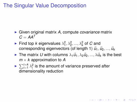
The Singular Value Decomposition
I Given original matrix A, compute covariance matrixC = AAT
I Find top k eigenvalues λ21, λ
22, ..., λ
2k of C and
corresponding eigenvectors (of length 1) ~u1, ~u2, ..., ~uk
I The matrix U with columns λ1~u1, λ2~u2, ..., λ~uk is the bestm × k approximation to A
I∑i=k
i=1 λ2i is the amount of variance preserved after
dimensionality reduction
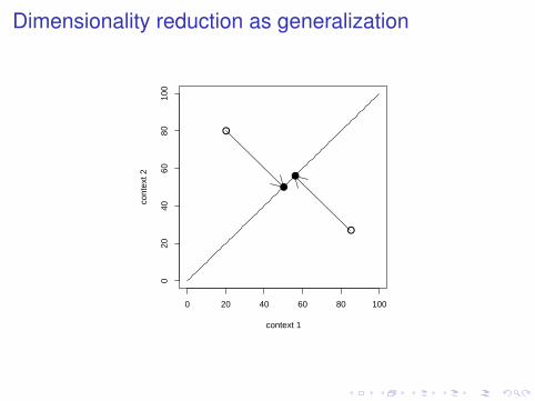
Dimensionality reduction as generalization
0 20 40 60 80 100
020
4060
8010
0
context 1
cont
ext 2●
●
●
●

Dimensionality reduction as generalization
buy sell dim1wine 31.2 27.3 41.3beer 15.4 16.2 22.3car 40.5 39.3 56.4cocaine 3.2 22.3 18.3

Interpreting the latent dimensions
I Not too transparent, they seem to capture broadsemantic/topical areas
I Words with highest positive and negative values on 2randomly picked dimensions of a BNC-trainedwindow-based semantic space (Baroni & Lenci in press):
Dim Top words Bottom words5 political, rhetoric, ideology, around, average, approximately,
thinking, religious compare, increase15 juice, colouring, dish police, policeman, road
cream, salad drive, stop

SVD: Empirical assessment
I In general, SVD really boosts performance (see, e.g., theclassic LSA work, Schütze 1997, Rapp 2003, Turney2006. . . )
I Results from our experiments with ukWaC-traineddependency-filtered model on next slide (fromHerdagdelen et al 2009)
I Picked top 300 latent dimensions

Classic semantic similarity taskswith and without SVD reduction
task with withoutSVD SVD
RG 0.798 0.689AP Cat 0.701 0.704
Hodgsonsynonym 10.015 6.623coord 11.157 7.593antonym 7.724 5.455conass 9.299 6.950supersub 10.422 7.901phrasacc 3.532 3.023

SVD and data sparseness
I The smoothing provided by SVD is sometimes (e.g., byManning & Schütze) argued to help attenuating theproblem of data sparseness
I As corpus size decreases, words are less likely to occur inthe very same contexts, but if they occur in globally similarcontexts, SVD might capture their similarity
I In Herdagdelen et al (2009), we investigated robustness ofSVD against data sparseness by re-training the models ondown-sampled versions of ukWaC source corpus: 0.01%(about 2 million words), 1% (about 20 million words), 10%(about 200 million words)

Performance after down-samplingPercentage proportion of full set performance
0.1% 1% 10%svd no svd svd no svd svd no svd
RG 0.219 0.244 0.676 0.700 0.911 0.829AP Cat 0.379 0.339 0.723 0.622 0.923 0.886synonym 0.369 0.464 0.493 0.590 0.857 0.770antonym 0.449 0.493 0.768 0.585 1.044 0.849conass 0.187 0.260 0.451 0.498 0.857 0.704coord 0.282 0.362 0.527 0.570 0.927 0.810phrasacc 0.268 0.132 0.849 0.610 0.920 0.868supersub 0.313 0.353 0.645 0.601 0.936 0.752

SVD: Pros and cons
I Pros:I Good performanceI At least some indication of robustness against data
sparsenessI Smoothing as generalization
I Hare (2006): use SVD to smooth across textual and visualfeatures, generalizing from captioned images to unannotatedones
I Cons:I Non-incremental (SVD done once and for all on the full
co-occurrence matrix)I Latent dimensions are difficult to interpretI Does not scale up well
I In my experience, problems SVD-ing matrices with over20K × 20K dimensions

Outline
Building the model
Weighting dimensions
Cosine similarity
Dimensionality reductionSingular Value DecompositionRandom Indexing

Random Indexing: The low-cost alternativeSahlgren 2005
I A pure dimensionality reduction technique (no “latentsemantics” effect)
I No need to build the full co-occurrence matrixI Given m target words and the intended number of
dimensions k , start and end with an m × k matrix, for apre-determined k , independently of number n ofconsidered contexts

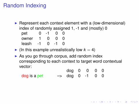
Random Indexing
I Represent each context element with a (low-dimensional)index of randomly assigned 1, -1 and (mostly) 0pet 0 -1 0 0owner 1 0 0 0leash -1 0 -1 0
I (In this example unrealistically low k = 4)
I As you go through corpus, add random indexcorresponding to each context to target word contextualvector:
dog 0 0 0 0dog is a pet –> dog 0 -1 0 0owner of the dog –> dog 1 -1 0 0dog on the leash –> dog 0 -1 -1 0

Random Indexing
I Represent each context element with a (low-dimensional)index of randomly assigned 1, -1 and (mostly) 0pet 0 -1 0 0owner 1 0 0 0leash -1 0 -1 0
I (In this example unrealistically low k = 4)I As you go through corpus, add random index
corresponding to each context to target word contextualvector:
dog 0 0 0 0
dog is a pet –> dog 0 -1 0 0owner of the dog –> dog 1 -1 0 0dog on the leash –> dog 0 -1 -1 0

Random Indexing
I Represent each context element with a (low-dimensional)index of randomly assigned 1, -1 and (mostly) 0pet 0 -1 0 0owner 1 0 0 0leash -1 0 -1 0
I (In this example unrealistically low k = 4)I As you go through corpus, add random index
corresponding to each context to target word contextualvector:
dog 0 0 0 0dog is a pet
–> dog 0 -1 0 0owner of the dog –> dog 1 -1 0 0dog on the leash –> dog 0 -1 -1 0
Random Indexing
I Represent each context element with a (low-dimensional)index of randomly assigned 1, -1 and (mostly) 0pet 0 -1 0 0owner 1 0 0 0leash -1 0 -1 0
I (In this example unrealistically low k = 4)I As you go through corpus, add random index
corresponding to each context to target word contextualvector:
dog 0 0 0 0dog is a pet –> dog 0 -1 0 0
owner of the dog –> dog 1 -1 0 0dog on the leash –> dog 0 -1 -1 0

Random Indexing
I Represent each context element with a (low-dimensional)index of randomly assigned 1, -1 and (mostly) 0pet 0 -1 0 0owner 1 0 0 0leash -1 0 -1 0
I (In this example unrealistically low k = 4)I As you go through corpus, add random index
corresponding to each context to target word contextualvector:
dog 0 0 0 0dog is a pet –> dog 0 -1 0 0owner of the dog
–> dog 1 -1 0 0dog on the leash –> dog 0 -1 -1 0

Random Indexing
I Represent each context element with a (low-dimensional)index of randomly assigned 1, -1 and (mostly) 0pet 0 -1 0 0owner 1 0 0 0leash -1 0 -1 0
I (In this example unrealistically low k = 4)I As you go through corpus, add random index
corresponding to each context to target word contextualvector:
dog 0 0 0 0dog is a pet –> dog 0 -1 0 0owner of the dog –> dog 1 -1 0 0
dog on the leash –> dog 0 -1 -1 0

Random Indexing
I Represent each context element with a (low-dimensional)index of randomly assigned 1, -1 and (mostly) 0pet 0 -1 0 0owner 1 0 0 0leash -1 0 -1 0
I (In this example unrealistically low k = 4)I As you go through corpus, add random index
corresponding to each context to target word contextualvector:
dog 0 0 0 0dog is a pet –> dog 0 -1 0 0owner of the dog –> dog 1 -1 0 0dog on the leash
–> dog 0 -1 -1 0

Random Indexing
I Represent each context element with a (low-dimensional)index of randomly assigned 1, -1 and (mostly) 0pet 0 -1 0 0owner 1 0 0 0leash -1 0 -1 0
I (In this example unrealistically low k = 4)I As you go through corpus, add random index
corresponding to each context to target word contextualvector:
dog 0 0 0 0dog is a pet –> dog 0 -1 0 0owner of the dog –> dog 1 -1 0 0dog on the leash –> dog 0 -1 -1 0

Random Indexing
I With a reasonably large k (a few thousands dimensions),good low dimensionality approximation of fullco-occurrence matrix
I Cosine similarity (or other similarity measure) computed onresulting contextual vectors

Pros and cons
I Pros:I Very efficient: low dimensionality from the beginning to the
end, independently of number of contexts taken intoaccount
I This will become more and more important as we work withlarger and larger corpora, richer contexts, etc.
I Implementation trivial (assign random values to vector, sumvectors)
I Incremental: at any stage, target vectors constitutelow-dimensional semantic space
I Cons:I No latent semantic space effect: contexts are “squashed”
randomlyI Multiple-pass Random Indexing? Perform SVD on RI output?
I Lower accuracy, at least on some tasks (Gorman andCurran 2006)