i

DISTRIBUTION SYSTEM MODELING FOR ASSESSING IMPACT OF SMART

INVERTER CAPABILITIES

by

Stephen Abate

BS, Electrical Engineering, Lehigh University, 2011

Submitted to the Graduate Faculty of

Swanson School of Engineering in partial fulfillment

of the requirements for the degree of

Master of Science

University of Pittsburgh

2015

ii

UNIVERSITY OF PITTSBURGH

SWANSON SCHOOL OF ENGINEERING

This thesis was presented

by

Stephen R. Abate

It was defended on

March 26, 2015

and approved by

Zhi-Hong Mao, PhD, Associate Professor, Electrical and Computer Engineering Department

Gregory F Reed, PhD, Associate Professor, Electrical and Computer Engineering Department

Thesis Advisor: Tom McDermott, PhD, Assistant Professor, Electrical and Computer

Engineering Department

iii

Copyright © by Stephen R. Abate

2015

iv

Photovoltaic (PV) generation is increasingly common throughout power distribution

systems. The real power injections and cloud-induced power output fluctuations of this variable

resource can cause adverse impacts to the system. These adverse impacts limit PV capacity

additions and introduce the need for more advanced distribution system models and mitigation

efforts. The IEEE P1547a standard for interconnecting distributed generation has been amended

to allow inverter-based generation to actively participate in voltage regulation. [1]

However, there is currently no method of choosing the appropriate reactive power response

for the PV inverters to prevent voltage issues and benefit distribution system performance. The

performance of these smart inverter settings vary based on the objective and system conditions

such as load level and solar conditions. This difficulty in choosing a single “out of the box” setting

presents the need for more adaptive control functionalities.

This thesis assesses the impact of different smart inverter settings on the performance of a

distribution feeder in the United States. The use of simulation software to identify relationships

between the chosen objective, appropriate settings, and feeder conditions help determine an

approach to choosing settings that realize the potential benefits. Due to the limitations of existing

reactive power control functions, a new smart inverter capability is proposed that adjusts to

changing feeder conditions and offers improved performance.

DISTRIBUTION SYSTEM MODELING FOR ASSESSING IMPACT OF

SMART INVERTER CAPABILITIES

Stephen R. Abate, M.S.

University of Pittsburgh, 2015

v

TABLE OF CONTENTS

ACKNOWLEDGEMENTS ........................................................................................................ X

1.0 INTRODUCTION ........................................................................................................ 1

1.1 POWER SYSTEM OVERVIEW ....................................................................... 2

1.1.1 Generation ........................................................................................................ 3

1.1.2 Transmission .................................................................................................... 3

1.1.3 Distribution ...................................................................................................... 5

1.2 DISTRIBUTED ENERGY RESOURCES ........................................................ 8

1.3 ADVERSE IMPACTS OF PV ............................................................................ 9

1.4 DISTRIBUTION SYSTEM MODELING ....................................................... 12

1.4.1 OpenDSS Model Structure ........................................................................... 13

1.4.2 Load Flow in OpenDSS ................................................................................. 14

1.4.3 Example OpenDSS simulations .................................................................... 16

1.5 DISTRIBUTION SYSTEM PERFORMANCE METRICS .......................... 19

1.5.1 Losses .............................................................................................................. 20

1.5.2 Voltage Regulator Tap Operations .............................................................. 20

1.5.3 Consumption .................................................................................................. 21

1.5.4 Voltage Variability Index .............................................................................. 22

1.6 SMART INVERTERS....................................................................................... 23

vi

1.6.1 Role of Inverter Rating ................................................................................. 24

1.6.2 Volt-var Response .......................................................................................... 26

2.0 VOLT-VAR SETTING PERFORMANCE ............................................................. 29

2.1 FEEDER MODEL ............................................................................................. 29

2.2 DAY CLASSIFICATION ................................................................................. 30

2.2.1 Solar Categorization ...................................................................................... 31

2.2.2 Load Categorization ...................................................................................... 32

2.2.3 Test Day Selection .......................................................................................... 32

2.3 VOLT-VAR SETTINGS ................................................................................... 33

2.4 RESULTS ........................................................................................................... 34

2.4.1 Losses .............................................................................................................. 35

2.4.2 Consumption .................................................................................................. 36

2.4.3 Number of Regulator Tap Changes ............................................................. 38

2.4.4 Voltage Variability Index .............................................................................. 38

2.5 VOLT-VAR LIMITATIONS ........................................................................... 39

3.0 DYNAMIC VREG SMART INVERTER ................................................................... 43

3.1 SIMULINK MODEL......................................................................................... 44

3.1.1 Load-flow Simulation .................................................................................... 45

3.1.2 Static volt-var simulation .............................................................................. 49

3.1.3 Dynamic Vreg voltvar simulation .................................................................. 51

3.2 ADVANTAGES OF DYNAMIC VOLT-VAR ................................................ 53

3.2.1 Improved Performance ................................................................................. 53

3.2.2 Automatic Setting Selection .......................................................................... 54

vii

3.2.3 Reactive Demand ........................................................................................... 54

4.0 CONCLUSION ........................................................................................................... 56

BIBLIOGRAPHY ....................................................................................................................... 57

viii

LIST OF FIGURES

Figure 1 - Transmission tower ........................................................................................................ 4

Figure 2 - Transmission tower ........................................................................................................ 5

Figure 3 - Distribution three-phase primary ................................................................................... 6

Figure 4 - Split-phase secondary diagram ...................................................................................... 7

Figure 5 - Distribution transformer from one primary phase to split-phase secondary .................. 7

Figure 6 - Distribution primary feeding three-phase secondary ..................................................... 8

Figure 7 - Simple Thévenin equivalent with real/reactive power PV injections .......................... 10

Figure 8 - OpenDSS Architecture [15] ......................................................................................... 13

Figure 9 - Peak and off-peak example loadshapes ........................................................................ 15

Figure 10 - Example PV power generation curve ......................................................................... 16

Figure 11 - Example load flow solution illustrated in a circuit diagram ...................................... 17

Figure 12 - Load flow solution illustrated in a voltage profile plot .............................................. 18

Figure 13 - Example time-series voltage plot ............................................................................... 19

Figure 14 - Diagram of a voltage regulator .................................................................................. 21

Figure 15 - Voltage Variability Index of an example signal ........................................................ 22

Figure 16 - Required inverter rating dependence on system X/R ratio ........................................ 26

Figure 17 - Volt-var curve ............................................................................................................ 27

Figure 18 - Classification of solar day based on clearness index and variability index ............... 31

ix

Figure 19 - Distribution of average daily load divided into three categories ............................... 32

Figure 20 - Solar classification with test days shown in red......................................................... 33

Figure 21 - Volt-var curves with variations in Vreg (top) and droop (bottom) ............................ 34

Figure 22 - Losses by setting for three overcast solar days .......................................................... 36

Figure 23 – Consumption by setting for three mild solar days ..................................................... 37

Figure 24 - Number of regulator tap changes by setting: high load, high variability day ............ 38

Figure 25 - Voltage Variability Index by setting for a high load, high variability solar day ....... 39

Figure 26 - Load and solar shape for a high load, high variability solar day ............................... 41

Figure 27 - VVI by setting for four smaller periods throughout the day ...................................... 42

Figure 28 - Full Simulink Model .................................................................................................. 44

Figure 29 - Simple Thévenin equivalent ....................................................................................... 45

Figure 30 - Simulink Load Flow solver ........................................................................................ 46

Figure 31 - Voltage at PCC without PV ....................................................................................... 47

Figure 32 - PV generation curve ................................................................................................... 48

Figure 33 - PCC Voltage (Unity PF) ............................................................................................ 49

Figure 34 - Volt-var response in Simulink ................................................................................... 49

Figure 35 - PCC Voltage with static volt-var implementation ..................................................... 50

Figure 36 - Simulink block diagram showing dynamic Vreg control .......................................... 51

Figure 37 - Vreg tracking to a step-input (top) and load flow (bottom) ....................................... 52

Figure 38 - Voltage PCC using different inverter settings ........................................................... 53

Figure 39 - Comparison of rating usage for static volt-var (left) and dynamic volt-var (right) ... 55

x

ACKNOWLEDGEMENTS

I would like to first thank my parents for their ongoing support of my educational pursuits,

career choices, and emotional well-being. It is impossible to list the sacrifices they have made to

give me the opportunity to be here pursuing and obtaining an advanced degree in electrical

engineering.

I would like to thank Dr. Tom McDermott for hiring me as his graduate student, providing

me with an enormous amount of technical and professional direction, and for being the largest

contributor to this thesis. It is truly inspiring to work closely with someone with such technical

expertise and success in the industry who is so humble and considerate. I am grateful for my

experience working for him and I hope to cultivate these qualities within myself as I continue to

grow personally and professionally. I would like to thank Dr. Gregory Reed for fostering a

tremendous learning environment in the research group and for being an important professional

role model to me. I would also like to thank Dr. Mao for his guidance and support through my

coursework and research. Even a brief remembrance of his enthusiasm in the classroom will

always remind me of the reasons why I chose the career that I did.

I would like to thank Matt Rylander and Jeff Smith at the Electric Power Research Institute

(EPRI) for advising me through my summer internship and graduate studies. The summer

experience and funding support provided by EPRI has proven to be a fundamental part of my

xi

graduate experience. Also, I would like to thank Roger Dugan and Mark McGranaghan at EPRI

for their professional and personal guidance.

I would like to thank Timothy Croushore at the FirstEnergy Technologies group for his

strong leadership in advising the Distribution Feeder Analytics project. The opportunity to work

with real utility data is rare for students and I truly appreciate the experience provided by

FirstEnergy. I would also like to thanks Dean Philips, Justin Price, and Mark Josef of the

FirstEnergy Distribution Planning group for being industry mentors that have introduced me to

practical considerations of distribution modeling and planning.

Finally, I would like to thank my fellow graduate student researchers, particularly Augustin

Crémer and Andrew Reiman, for the essential comradery that made our hard work fulfilling and

enjoyable.

1

1.0 INTRODUCTION

The United States is experiencing persistent growth in total photovoltaic (PV) capacity

with expected new installations reaching almost 9,000 MW in the year 2015 [2]. Scheduled

capacity additions consist largely of renewable resources while fossil fuel based generation is

anticipating increased retirement. [3] This larger reliance on variable, weather-dependent, and

distributed generation in place of traditional sources will introduce complications in the operation

of distribution systems.

Local power system impact is considerable in areas where PV capacity exceeds 10% of a

typical day’s peak load as seen in California and Hawaii. [4] These issues have brought increased

attention to developing more advanced distribution system modeling tools and methods. [5] Some

voltage issues caused by PV can be mitigated by operating the PV inverters to absorb or inject

reactive power. The reactive power capabilities of these “smart inverters” include operating in an

off-unity power factor or in a control mode where reactive power is dependent on voltage (volt-

var mode).

The utility industry is moving toward the adoption of these reactive power control

capabilities of inverters in order to improve power system performance and increase hosting

capacity. The IEEE 1547 standard for interconnecting distributed generation has recently been

amended to allow inverter-based generation to actively participate in voltage regulation. [1] Also,

2

some proactive measures to update interconnection requirements, such as California Rule 21, have

been made to adopt these reactive power capabilities in order to meet solar installation targets. [6]

However, there is currently no methodology to properly select smart inverter settings and

fully achieve the benefits to distribution feeder performance. Feeder objectives are competing and

have an unclear relationship to the appropriate settings. Furthermore, settings that improve

performance for one feeder condition will produce different results when varying solar output

characteristics or load level. [7]

This thesis assesses the impact of different volt-var settings on distribution system

performance using simulation software to identify relationships between the chosen objective and

appropriate settings for different feeder conditions. The model of this feeder makes use of

historical data to simulation actual system conditions. Limitations of volt-var capabilities are

discussed and a new reactive power control method is introduced. This new control structure is

shown to have improved performance and robustness in setting selection.

1.1 POWER SYSTEM OVERVIEW

The traditional power system consists of bulk power generation that is transported via conductors

at various voltage levels in order to deliver electricity to customers. The infrastructure and

operation of this “grid” can roughly be categorized into three stages: Generation, Transmission,

and Distribution. The electric power produced by the generation source is stepped-up to a higher

voltage that is more suitable for long-distance transmission. This power then enters various stages

3

of voltage transformations (sometimes considered sub-transmission) before reaching the

distribution voltage and eventually the nominal customer voltage.

1.1.1 Generation

Electricity generation relies on different methods of converting sources of energy into electrical

energy. Whether converting heat energy (coal, nuclear, etc.) or kinetic energy (wind, hydro), most

generators involve some sort of electromagnetic-mechanical energy conversion process. Other

processes such as electro-chemical (batteries) and the photovoltaic effect (solar cells) are used to

produce electricity. In 2013, the generation capacity of the United States consisted mostly of coal

(39%), natural gas (26%), and nuclear (19%). [8] However, scheduled capacity installations and

retirements predict a greater dependency on renewables sources such as wind and solar in the

future. [3]

1.1.2 Transmission

The power from the generator enters a step-up transformer, where it can be transported at a high

voltage via transmission lines. Typical transmission voltage levels fall between 138 kV and 765

kV. The high voltage is favorable for long-distance transportation of power due to the lower

currents and consequently lower resistive (i2R) losses. The main cause of transmission failures

are lightning and other weather-related events. [9] Figure 1 and Figure 2 show pictures of

transmission towers found in the Pittsburgh area.

4

Figure 1 - Transmission tower

5

Figure 2 - Transmission tower

1.1.3 Distribution

The transmission system provides power to the distribution stage of the system through distribution

substations that serve to step down and regulate voltages while isolating faults. Typical

distribution voltages range from 2 kV to 35 kV to provide an economical balance between system

losses and cost of required equipment. Common causes of outages include vegetation, animals,

and lightning. Figure 3 shows a distribution pole carrying a three-phase primary (at the top of the

pole).

6

Figure 3 - Distribution three-phase primary

When the distribution line approaches the customer location, the voltage is stepped down

one final time to the nominal load voltage level (secondary). For residential customers, this would

require a split-phase secondary connection as shown in Figure 4. This three-wire connection with

a grounded neutral center tap from the distribution transformer allows for smaller conductor sizes

and provides two voltage levels for customers. Most household appliances are connected (and

balanced) to the 120 V sources, while other larger loads, such as cooking equipment and air

conditioners, are tied to the 240 V connection. Figure 5 shows one primary phase connected to a

distribution transformer that feeds a split-phase secondary circuit. Distribution transformers may

also feed three-phase secondary circuits for larger customer loads, as shown in Figure 6.

7

Figure 4 - Split-phase secondary diagram

Figure 5 - Distribution transformer from one primary phase to split-phase secondary

8

Figure 6 - Distribution primary feeding three-phase secondary

1.2 DISTRIBUTED ENERGY RESOURCES

The traditional power system, in concept, assumes one-way power flow from the bulk generation

source to the customer load. However, increasing interest from the Department of Energy and

regulators have resulted in a push for utilities to accommodate customers with generation

capabilities. Because customers are scattered throughout the distribution network, this approach

introduces challenges to existing systems, which are designed for the traditional one-way power

flow. Furthermore, these distributed generators are typically renewable sources with variable

generation levels, which depend on weather events that are difficult to predict.

9

In addition to the expected increase of residential solar penetration and impact on the

distribution system, the scheduled 2015 capacity additions according to the United States Energy

Information Administration (EIA) include 2,235 MW of solar and 9,811 MW of wind. [3] The

majority of these solar additions are utility-scale and will be installed in California and North

Carolina. The new additions will required additional simulation tools and approaches to successful

accommodation.

1.3 ADVERSE IMPACTS OF PV

The increased penetration of distribution energy resources, such as PV, will have a number

of adverse impacts on distribution systems. Exceeding the thermal rating, or maximum current

carrying capacity, of devices installed on the distribution system is another adverse impact to PV

installations. At minimum load and maximum generation, the PV can increase the amount of

current flowing through system devices that may not be adequately rated. Furthermore, the

increased current capacity may increase fault current level beyond the level prohibited by the

existing circuit breakers. [10] Also, voltage regulating devices, depending on the voltage control

scheme, may malfunction in response to reverse power flow.

PV generation tends to have high ramp rates, intermittency, and unpredictable fluctuations,

which pose an increased threat as penetration levels become higher. Specifically, PV power can

drop from 100% to 20% of nameplate capacity in less than one minute. [11] These fluctuations

cause an increased number of capacitor switches and regulator tap operations, reducing equipment

life. [12]

10

The voltage impact due to real and reactive power injections of a PV inverter can

approximated by examining the simple Thévenin equivalent shown in Figure 7.

Figure 7 - Simple Thévenin equivalent with real/reactive power PV injections

𝐼𝑛 =𝑃𝑛 − 𝑗𝑄𝑛

𝑉𝑁∗ (1)

𝑉𝑛 = 𝑉𝑔 + 𝑉dro𝑝 (2)

𝑉𝑑𝑟𝑜𝑝 = 𝑉𝑛 − 𝑉𝑔 = (𝑅 + 𝑗𝑋)𝐼𝑛 =1

𝑉𝑛∗

[(𝑅𝑃𝑛 + 𝑋𝑄𝑛) + 𝑗(𝑋𝑃𝑛 − 𝑅𝑄𝑛)] (3)

Equation (3) can be simplified using the following assumptions:

1. The reactive drop is negligible because the X/R ratio is closer to 1 on

distribution systems than on transmission systems.

𝑋𝑃𝑛 − 𝑅𝑄𝑛 ≅ 0 (4)

2. The voltage phase shift is negligible due to the low distribution system

reactance.

𝑉𝑛

∗ ≅ 𝑉𝑛 (5)

11

3. The source voltage (Vg) is constant

Incorporating these three assumptions result in Equation (6) and the partial derivative

approximations (7) and (8) below:

𝑉𝑛 − 𝑉𝑔 ≅1

𝑉𝑛

[𝑅𝑃𝑛 + 𝑋𝑄𝑛] (6)

𝜕𝑉𝑛

𝜕𝑃𝑛≅

𝑅

𝑉𝑛 (7)

𝜕𝑉𝑛

𝜕𝑄𝑛≅

𝑋

𝑉𝑛 (8)

These partial derivatives are used to form Equation (9) below, which approximates the

voltage rise (ΔVn) due to PV real power (ΔPn) and reactive power (ΔQn) injections. The voltage

impact of the PV installations is large for weak systems (i.e. high Thévenin impedance) but also

allows for greater influence of the inverter reactive power capabilities.

∆𝑉𝑛 ≅𝑅

𝑉𝑛∆𝑃𝑛 +

𝑋

𝑉𝑛∆𝑄𝑛 (9)

12

1.4 DISTRIBUTION SYSTEM MODELING

Distribution system models traditionally have been used to plan new distribution circuits,

accommodate additional customers, and address voltage issues. [13] However, distribution

planning for PV requires more advanced studies and models as opposed to simple assessments of

loading conditions. [14] Proper assessment of distributed energy resource impact and performance

requires modeling tools that can simulate the varying conditions that these resources imposes on

the distribution system.

OpenDSS is an open-source electric power Distribution System Simulator (DSS)

maintained by the Electric Power Research Institute (EPRI). Its diverse capabilities range from

general distribution planning and analysis, to renewable integration and load/storage simulators.

In 2008, EPRI released the program under an open source license, meaning that additional

functionality can be added as necessary to support new developments and technologies. One of

the unique aspects of OpenDSS is that it never makes internal simplifications related to phase

balance or symmetrical components. The Windows Component Object Model (COM) interface

allows for scripted simulations that can be used to perform various tests under different feeder

conditions. In this study, the COM interface is used with MATLAB to compare the performance

of various PV inverter settings for regulating local voltage. The following sections describe the

structure of OpenDSS models, the solution process, and an example model of a distribution circuit

in the United States.

13

1.4.1 OpenDSS Model Structure

An OpenDSS model typically consists of a “main” DSS script, supporting scripts, and

supporting files (such as comma-separated value files for load shapes). The “main” DSS script

will redirect to the other DSS files that focus on a particular part of the circuit. For example, it is

convenient to place all load declarations in a single “loads.dss” file in order to manage the large

number of declarations associated with a distribution circuit. Figure 8 illustrates the OpenDSS

architecture including the five classes of circuit elements. The Power Delivery Elements

(PDElement), such as transformers and lines, serve to convert energy from one set of terminals to

another. Power Conversion Elements (PCElement), such as loads and generators, convert

electrical energy to other forms of energy (or vice-versa). The Controls class includes voltage

regulator controls, capacitor switching settings, and inverter control schemes. Meters are used to

record and export model data during simulations. The General class contains other supporting

data structures, such as conductor parameters, transformer models, and load shapes.

Figure 8 - OpenDSS Architecture [15]

14

The OpenDSS model used in this project includes substation power, modeled as a stiff

source, along with distribution system components, including conductors, transformers, regulators,

capacitors, and other interconnecting components. Constant power loads are defined at each time

step by a load shape, which can be based on measurements taken at the substation. Distributed

energy resources can be modeled as constant power generators with or without a load shape. Loads

and distributed energy resources are connected to service points on the secondary side of

distribution transformers.

1.4.2 Load Flow in OpenDSS

The objective of solving the load flow problem is to determine the voltage, current, and

power phasors throughout the entire power system. Originally designed for harmonic flow

analysis of large, arbitrarily-meshed, multi-phase networks, OpenDSS is more powerful than most

basic load flow solvers. [15] Other load flow solvers are formulated under the assumption that

the distribution circuit is balanced, radial, and weakly-meshed. The OpenDSS solver will

construct a primitive admittance matrix for each current-carrying element, form the system nodal

admittance matrix, and iterate to solve the matrix equation that describe the flow of power in the

system.

The simplest solution mode of OpenDSS is the “snapshot” mode which solves a single

load-flow problem at a single point in time. Another solution mode that is particularly useful in

assessing PV impact is the quasi-static time-series simulations. In this mode, the simulation keeps

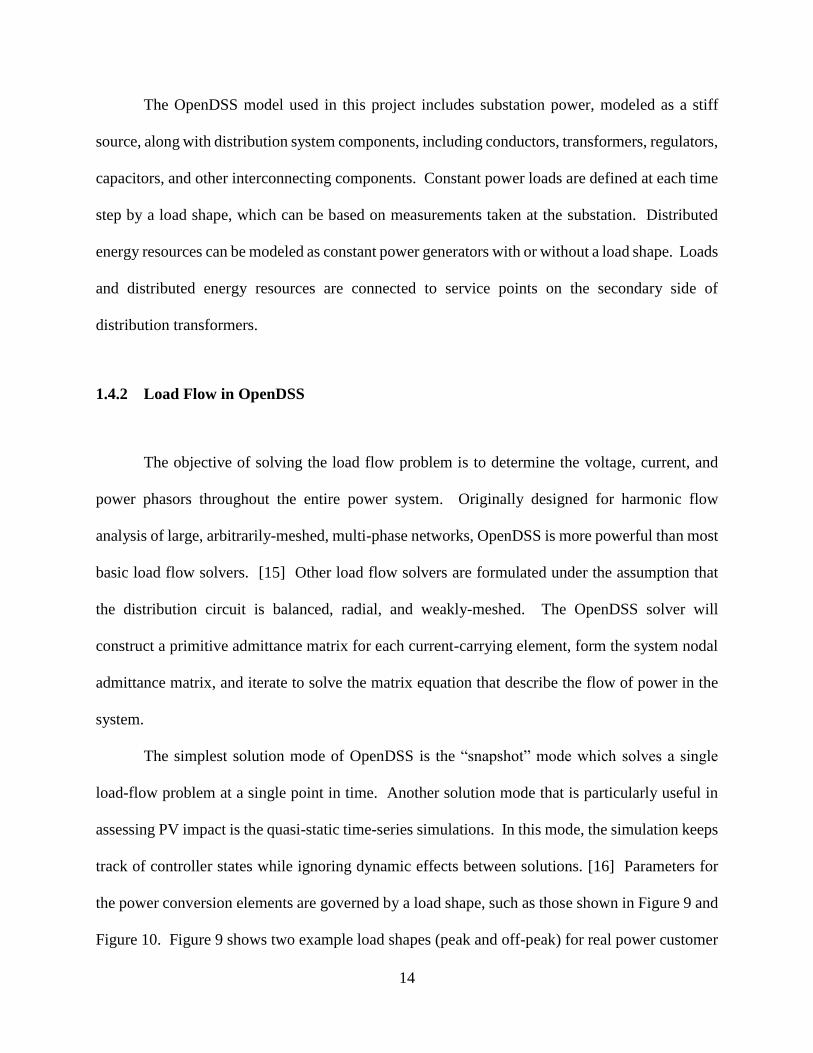
track of controller states while ignoring dynamic effects between solutions. [16] Parameters for

the power conversion elements are governed by a load shape, such as those shown in Figure 9 and

Figure 10. Figure 9 shows two example load shapes (peak and off-peak) for real power customer

15

load consumption and Figure 10 shows an example PV power output curve representing a day with

cloud-induced power-output swings.

The step-size of the time-series simulation can be as short as a few cycles to as long as a

day or more. When the time-series step-size is less than that of a load shape, OpenDSS will linearly

interpolate the load shape to determine the appropriate parameter.

Figure 9 - Peak and off-peak example loadshapes

0 5 10 15 20 250.1

0.2

0.3

0.4

0.5

0.6

0.7

0.8

0.9

1

Time (hr)

Load (

p.u

. m

ax)

Peak

Offpeak

16

Figure 10 - Example PV power generation curve

For a single snapshot or individual time-step, load flow solutions are performed while

iterating through controlled component settings until a solution is found that satisfies all controlled

component requirements. Controlled components can include voltage regulators, capacitors and

distributed energy resources. Individual load flow solutions are fast enough that iterating through

several hundred time-steps completes in a matter of seconds.

1.4.3 Example OpenDSS simulations

The outputs of a load-flow solution include the voltage, current, and power phasors

throughout the system. OpenDSS can use this information to generate plots that provide a

visualization of the load flow solution. For example, Figure 11 shows an example of a snapshot

load flow for a feeder in the United States. The thickness of a line segment is proportionate to the

0 5 10 15 20 25-0.2

0

0.2

0.4

0.6

0.8

1

1.2

Time (hr)

Pow

er

(per-

unit r

ating)

17

percentage of rated power flowing through that segment. The substation can be identified by the

thickest line segment in the plot above. This feeder is sourced by a single substation located at the

bottom of the figure. The thinner blue line segments correspond to lower power flow and can be

found at the end of the distribution system. The x-axis and y-axis are linearly related to longitude

and latitude, respectively.

Figure 11 - Example load flow solution illustrated in a circuit diagram

Another useful plot that illustrates the solution of the load flow problem is the voltage

profile. The voltage profile shows the system voltages versus the (electrical) distance from the

substation. An example voltage profile from a modeling effort for the EPRI Smart Grid

Demonstration Initiative is shown in Figure 12. [5] The black, red, and blue lines indicate the

primary Phase A, Phase B, and Phase C voltages respectively. The dotted lines represent the

18

secondary circuit. Customer loads and associated distribution transformers bring the voltage down

throughout the feeder.

The American National Standards Institute (ANSI) C84.1 establishes the nominal voltage

ratings and operating tolerances for 60-Hz electric power systems. Specifically, voltages that are

beyond ±5% of nominal system voltage (A range) are considered violations to utilities. In addition

to making ANSI violations apparent, the voltage profile can show the configuration of system

devices, such as capacitor or line regulators. In this case, the voltage regulators are tapping the

voltage up, which causes the discontinuities in the plot.

Figure 12 - Load flow solution illustrated in a voltage profile plot

19

The results of a quasi-static time-series solution is shown in Figure 13. This simulation is

designed to test the impact of a very large residential PV installed at the distribution secondary.

The plot shows that the voltage at the PV site exceeds the ANSI 1.05 p.u. (126 V) limit during

hours of peak generation; this suggests that infrastructure changes might be required to

accommodate this for this PV system.

Figure 13 - Example time-series voltage plot

1.5 DISTRIBUTION SYSTEM PERFORMANCE METRICS

When performing simulations using OpenDSS, there are a number of different metrics that are

useful in assessing the performance of the distribution system. [17] The load flow problem is

solved and the system currents, voltages, and power flows are available for further post-processing

and analysis. These flow variables and the physical devices they are associated with allow for the

20

computation of quantities such as system losses and customer consumption. Other metrics, such

as the number of capacitor bank and regulator tap operations, are recorded to quantify the strain

on these devices. The variability of system voltages (typically at the PV point of common

coupling) during a period of time can be quantified to assess PV impact.

1.5.1 Losses

Approximately two-thirds of the power system losses in the United States occur at the distribution

level. Losses that accumulate throughout the distribution system are caused primarily by resistive

elements of the power lines/transformers (I2R) and excessive reactive power flow. These losses

typically range from 3 to 10%, and this wasted energy is undesirable to regulators and society

because it reduces the efficiency of the system. In recent years, the goal of reducing losses and

incentivizing loss reduction has received additional attention from industry and regulators due to

increased environmental concerns. [18]

1.5.2 Voltage Regulator Tap Operations

Voltage regulators are devices that keep the distribution voltage within the appropriate range of

values needed to reduce voltage drops and ensure adequate voltage levels at the customer locations.

Typical voltage regulators are capable of adjusting the voltage by ±10% with 32 taps between the

minimum and maximum voltage level. [13] Figure 14 provides a simple diagram of the tapping

mechanism of a voltage regulator. The source could be a transmission or equivalent source and

the regulating bus would likely feed downstream loads. In reality, the tapping mechanism could

21

be based on an autotransformer winding configuration of the transformer; the role in maintaining

voltage is the same.

Figure 14 - Diagram of a voltage regulator

1.5.3 Consumption

Reducing overall consumption conserves energy and is a measure of feeder performance for

utilities. Utilities may be incentivized to minimize consumption for environmental reasons, but the

resulting increase in capacity to accommodate additional customers (presumably preventing

infrastructure costs) may make it a valuable objective in itself. This concept is known as

conservation voltage reduction (CVR), which relies on the fact that energy consumption of

customer loads decreases when voltages are at the lower acceptable limits. [19] CVR load models

are used in this feeder model to reflect the reduction in customer demand with decreasing voltage.

22

1.5.4 Voltage Variability Index

This metric is a modified version of the solar variability index (discussed in Section 2.2.3) used to

classify solar generation. Equation (10), which calculates the “length” of a voltage signal (see

Figure 15), is used to calculate the voltage variability:

∑ √(𝑉𝑘 − 𝑉𝑘−1)2 + ∆𝑡2

𝑛

𝑘=2 (10)

Where Vk is a sequence of voltage measurements sampled every Δt (in minutes). The quantity

will be larger for voltage signals that vary more throughout the duration of interest.

Figure 15 - Voltage Variability Index of an example signal

23

The voltage variability index is defined by the ratio of this quantity for two voltage measurements.

For example, it can be advantageous to compare voltage variability to that of the unity power factor

case (i.e. an index greater than 1 means more variability than with unity power factor), or to that

of the no PV case.

1.6 SMART INVERTERS

The Electric Power Research Institute (EPRI) has collaborated with individuals

representing inverter manufacturers in order to establish a common set of smart inverter functions.

These functions allow smart inverters to vary their real and reactive power output in response to

the system voltage [20]. The implementation of off-unity power factor settings in inverters proves

advantageous at lessening the voltage impact of PV generation. Other capabilities include the volt-

watt functionality, which will curb the real power injection in order to prevent excessive voltage

rise at the interconnection point. Volt-var functionality, the primary focus of this thesis, will vary

reactive power output in order to regulate the local voltage to an established voltage setpoint (Vreg).

This functionality is preferred to volt-watt because it does not require the curtailment of solar

power output to control voltage. The ability of the inverter to provide and absorb vars is dependent

upon the inverter rating.

24

1.6.1 Role of Inverter Rating

The rating of the PV inverter will determine the amount of vars that are available for

injection/absorption and consequently its limitations in regulating the system voltage. The amount

of vars available can be calculated beginning with Equation (11).

𝑆2 = 𝑃2 + 𝑄2 (11)

Assuming an inverter rating of 110% of maximum solar output [kW] and solving for Q leads to

Equation (12):

→ 𝑄 = ±√𝑆2 − 𝑃2 = ±𝑃√1.12 − 1 = ±.4583𝑃 (12)

This means that, for example, a PV system of rating 100 kW will have 45.83 kvars at its disposal

during peak hours of generation. At off-peak hours of generation, the inverter will have more vars

available since the real power output is less. The importance of the inverter rating can be

demonstrated in the selection of an off-unity power factor. As previously derived, in Section 1.3,

the following approximation in Equation (13) describes the change in voltage associated with real

and reactive power injections at a PV site.

∆𝑉𝑛 ≅𝑅

𝑉𝑛∆𝑃𝑛 +

𝑋

𝑉𝑛∆𝑄𝑛 (13)

Where R and X are the resistive and reactive components of the Thévenin equivalent impedance

and P and Q are the real and reactive power injections at the PV PCC. From here, setting ΔV=0,

we can approximate the reactive power output required to offset the real power rise in Equation

(14):

25

𝑅

𝑉𝑃 → 𝑄 = −

𝑅

𝑋𝑃 (14)

This leads to a derivation of the required power factor for a given system impedance (15):

pf =𝑃

|𝑆|=

𝑃

√𝑃2 + 𝑄2=

𝑃

𝑃√1 + (𝑅𝑋)

2=

1

√1 + (𝑅𝑋)

2

(15)

We can then determine the inverter rating (in percentage of PV rating) that is required to offset the

rise in voltage due to real power injections (17).

pf =𝑃

|𝑆| → |𝑆| =

𝑃

pf (16)

|𝑆|%req =|𝑆|

𝑃=

1

pf= √1 + (

𝑅

𝑋)

2

(17)

Figure 16 plots this expression and shows how the required inverter rating varies for different X/R

ratios. In comparison to transmission, the X/R ratio of a distribution system equivalent impedance

is relatively low (0.5 to 10). Figure 16 shows that for impedances with low X/R ratios, the inverter

rating may not be sufficient to offset the voltage rise due to real power injections. Specifically, a

110% ratio will only be sufficient for X/R ratios as low as approximately 2.18.

26

Figure 16 - Required inverter rating dependence on system X/R ratio

1.6.2 Volt-var Response

An inverter operating with the volt-var functionality will vary its reactive power output in

accordance with the volt-var curve shown in Figure 17.

0.5 1 1.5 2 2.5 31

1.5

2

2.5

X/R ratio

Required I

nvert

er

Rating (

S%

req)

110% Inverter Rating

27

Figure 17 - Volt-var curve

When voltage rises above the Vreg setting due to PV real power output increasing or feeder

events such as load dropping, the inverter will absorb reactive power (inductive region) to bring

the voltage closer to Vreg. Similarly, if voltage falls below Vreg, the inverter will provide reactive

power to boost the voltage closer to Vreg similar to a voltage-controlled capacitor bank. Note that

the vertical axis of the characteristic curve is an amount of reactive power in per-unit available

rather than an amount of reactive power in vars. The amount of available reactive power at a given

moment is dependent upon the PV real power output and the maximum apparent power rating of

the inverter, unless the inverter is operating in a mode that favors reactive power over real power.

The droop parameter, as described by Equation (18) below, quantifies how much reactive

power the inverter will provide or absorb per amount of voltage deviation from Vreg. For example,

if the droop parameter is 100 p.u. vars per p.u. volt, and the local voltage is less than Vreg by .01

p.u., the inverter will provide 100% of its available reactive power.

28

Droop ≔ −𝑑𝑄%𝑎𝑣𝑎𝑖𝑙

𝑑𝑉𝑝𝑢 (18)

29

2.0 VOLT-VAR SETTING PERFORMANCE

This section describes a set of simulations that was performed on a feeder in the United

States to assess the impact of volt-var settings on distribution performance. Previous work has

investigated the dependence of suitable volt-var settings on solar characteristics and load level

[7]. Some settings are best suited for the severity of cloud-induced power output swings, while

others perform best on clear days. The appropriate setting also has a heavy dependence on load

level. This study expands the number of setting groups, makes use of actual measured load and

solar data, and utilizes a method of categorizing days based on this data. Identifying key

relationships between the chosen objective, appropriate settings, and feeder variables aids in

determining a methodology to choose settings and fully realize the potential benefits. The

limitations of the volt-var functionality are also discussed, leading to the introduction of a new

and improved method.

2.1 FEEDER MODEL

The distribution feeder used in this study is an actual 12.47 kV feeder in the United

States. The feeder is part of a U.S. Department of Energy project and has been thoroughly

modeled and validated. Refer to [21] for a schematic of the feeder indicating regulators,

30

capacitors, and PV systems. Serving a peak load of 6 MW via 58 total three-phase and single-

phase feeder miles, this feeder covers a large footprint of almost 35 square miles. This feeder

also makes use of three banks of single-phase line regulators and five switched capacitor banks

totaling 3.9 Mvar. There is 1.7 MW of PV consisting of four large units at two locations, which

are approximately four feeder miles from the substation. There is also an additional 100 kW of

small residential systems throughout the feeder. For the purpose of isolating the problem of

setting selection for a single inverter, only one large PV system (760 kW out of 1.7 MW) is

active during the simulation.

The inverters are assumed to be rated 110% of the PV maximum dc output power.

Voltage regulation controls are implemented, which include the capacitor controls, substation

load tap changers, line drop compensators, and line regulators, and their respective setpoints (e.g.

voltage setpoints, voltage and current transformer ratios, bandwidths, delays, etc).

2.2 DAY CLASSIFICATION

The load shapes and solar generation curves used in the model were from actual

measurements between the dates April 6, 2012 and February 23, 2013. In order to cover the range

of possible feeder conditions, each day was categorized based on solar and load level.

31

2.2.1 Solar Categorization

The clearness index and variability index are used to choose the appropriate solar design day

categories. These two variables quantify irradiance variability in order to ensure the days chosen

for simulation cover the range of possibilities. The variability index is defined in Equation (19)

where the sequences GHI and CSI are the global horizontal irradiance and clear sky irradiance,

respectively, sampled every time Δt in minutes [22].

𝑉𝐼 =∑ √(𝐺𝐻𝐼𝑘 − 𝐺𝐻𝐼𝑘−1)2 + ∆𝑡2𝑛

𝑘=2

∑ √(𝐶𝑆𝐼𝑘 − 𝐶𝑆𝐼𝑘−1)2 + ∆𝑡2𝑛𝑘=2

(19)

The clearness index is defined as the ratio of solar energy measured on a given surface to

the theoretical maximum energy on that same surface during a clear sky day [23]. Figure 18 shows

the clearness index and variability index for the PV output on each of the 324 days, divided into

five categories.

Figure 18 - Classification of solar day based on clearness index and variability index

32

2.2.2 Load Categorization

For each of the five solar categories described above, three load categories are considered based

on the average daily load. Figure 19 shows a histogram of average daily loads throughout the 324-

day period. The load levels are created by establishing thresholds at 1/5 and 2/5 of the histogram

spread in order to achieve approximately equal occurrence probabilities among the load levels.

Figure 19 - Distribution of average daily load divided into three categories

2.2.3 Test Day Selection

Fifteen design days were chosen based on actual data using five solar categories and three load

levels to best represent the varying conditions of the feeder. Figure 20 shows each day (represented

33

by a circle) on the settings that were selected. For each solar category, there are three days selected

for low, medium, and high low levels.

Figure 20 - Solar classification with test days shown in red

2.3 VOLT-VAR SETTINGS

In this study, 75 total settings are investigated with 15 different Vreg choices between .98 and 1.05

and 5 different droop settings between 10 and 90, inclusive. Figure 21 illustrates example

variations in the setting parameters Vreg and Droop. These ranges are chosen based on knowledge

of previous work on the same feeder to surround the suspected optimal points.

0 5 10 15 20 25 30 350

0.2

0.4

0.6

0.8

1

1.2

Daily Variability Conditions

Variability Index

Cle

arn

ess I

ndex

34

Figure 21 - Volt-var curves with variations in Vreg (top) and droop (bottom)

2.4 RESULTS

Using the chosen settings and test days, the results were assessed for trends among the chosen

objective, load/solar conditions, and volt-var setting selection. There are noticeable trends in the

optimal Vreg setting with respect to the baseline (unity PF) average voltage. Also, the choice in

larger droop generally offers slightly better performance near the optimal points. However, the

larger the droop, the worse the performance is for settings with a poorly chosen Vreg.

0.94 0.96 0.98 1 1.02 1.04 1.06 1.08 1.1

-1

-0.5

0

0.5

1

Voltage (p.u.)

vars

(p.u

. availa

ble

) Voltvar Response

0.94 0.96 0.98 1 1.02 1.04 1.06 1.08 1.1

-1

-0.5

0

0.5

1

Voltage (p.u.)

vars

(p.u

. availa

ble

) Voltvar Response

35

2.4.1 Losses

Setting selection for decreasing losses results in a Vreg that is greater than the average PV output

voltage in the unity PF case as shown in Figure 22. The vertical black line and the horizontal green

line show the average voltage and losses, respectively, from the no PV case. From top to bottom,

the figure shows the losses for a low, medium, and high load day with a solar classification of

overcast. The voltage increase reduces the system current and therefore reduces the I2R losses.

36

Figure 22 - Losses by setting for three overcast solar days

2.4.2 Consumption

Setting selection for decreased consumption results in a Vreg that is less than the average PV

output voltage in the base case as shown in Figure 23. From top to bottom, the figure shows the

customer consumption for a low, medium, and high load day with a solar classification of

37

moderate. The reduction in voltage decreases customer demand. The medium load day

experiences an increase in consumption for settings with lower Vreg due to invoking capacitor and

regulator control actions that increase voltage at throughout the feeder.

Figure 23 – Consumption by setting for three mild solar days

38

2.4.3 Number of Regulator Tap Changes

When the reactive power capabilities of the inverters are utilized, the voltage fluctuations can be

lessened to increase asset life. Figure 24 shows the amount of regulator tap changes throughout

the day for different settings on a high load, high variability solar day. Typically, a setting with a

Vreg near the average voltage will reduce the voltage variability and consequently the number of

regulator tap changes.

Figure 24 - Number of regulator tap changes by setting: high load, high variability day

2.4.4 Voltage Variability Index

The improvement in the Voltage Variability Index is shown in Figure 25 for different settings on

a high load and high variability solar day. The vertical and horizontal green lines show the average

voltage and voltage variability, respectively, for the no PV case. The vertical and horizontal blue

lines show the average voltage and voltage variability, respectively, for the unity power factor

1 1.01 1.02 1.03 1.04 1.05

45

50

55

60

65

70

75

80

Vreg (V)

Num

ber

of

Regula

tor

Tap C

hanges

Droop: 10

Droop: 30

Droop: 50

Droop: 70

Droop: 90

39

case. The introduction of the PV real power injections increases both the average voltage and

voltage variability. When the appropriate volt-var setting is implemented, the local voltage

variability decreases below that of the unity power factor case. The appropriate setting has a Vreg

that is slightly higher than the average voltage.

Figure 25 - Voltage Variability Index by setting for a high load, high variability solar day

2.5 VOLT-VAR LIMITATIONS

Choosing an appropriate setting for one feeder condition will typically produce drastically

different results when varying the load level and solar characteristics. The feeder objectives tend

to be competing and have an unclear relationship to a single suitable setting. This means that volt-

var implementation would require some sort of communications infrastructure to update settings

based on forecasted load and solar information, which increases the cost and complexity. If the

inverters were to operate in an autonomous manner, it would difficult to establish a methodology

40

to properly choose an “out of the box” setting that benefits the feeder without any adverse effects.

The simulations have shown the consequences of implementing a poorly chosen volt-var setting

on the feeder objective.

Ideally, the volt-var control would adjust to a suitable setting upon startup, which would

relieve the end user of the burden of choosing a setting and adjusting it based on forecasted

information. The ability to adapt to the system conditions that affect the proper setting is essential

to fully realizing the benefits to distribution feeder performance.

The following two figures illustrate how the optimal setting shifts as the day progresses.

Figure 26 shows the load shape and solar generation curve for a day with high load and high solar

variability. The regions between the red lines correspond to the four plots in Figure 27 to show

how the settings that best reduce the voltage variability will change throughout the day. During

the first period, the volt-var capability will, at best, maintain variability equal to that of the no PV

case and will otherwise increase the variability. During the other periods, the best choice of Vreg

for improving variability fluctuates between 1.025 and 1.05.

41

Figure 26 - Load and solar shape for a high load, high variability solar day

0 500 1000 15001.5

2

2.5

3

3.5

4x 10

6 High Solar, High Load

Load (

W)

Time (min)

0 500 1000 1500-2

0

2

4

6

8x 10

5

Sola

r (W

)

Time (min)

42

Figure 27 - VVI by setting for four smaller periods throughout the day

43

3.0 DYNAMIC VREG SMART INVERTER

The volt-var response of PV inverters for regulating distribution system voltage is limited by a

lack of adaptation and methods for setting selection. Setting selection relies on properly choosing

the appropriate Vreg and droop parameters using a detailed feeder model, forecasted loading

levels, and the anticipated solar conditions. Furthermore, the ability to update the setting based on

the type of day requires a communication infrastructure. Consequently, an alternative control

strategy where the Vreg parameter dynamically responds to the system voltage is explored in this

section. The objective of this autonomous control strategy is to automatically adjust to the system

conditions on which the suitable settings depend. As previously discussed, the fluctuations in local

voltage due to cloud-induced power output swings can occur during the 1-minute timeframe. The

slower voltage fluctuations due to load changres occur during the 1-hour timeframe. The following

sections discuss the Simulink model that was developed to simulate a dynamic voltvar

implementation where the inverter setpoint follows the measured point of common coupling (PCC)

voltage.

44

3.1 SIMULINK MODEL

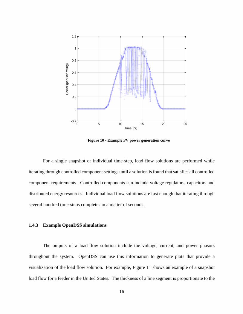
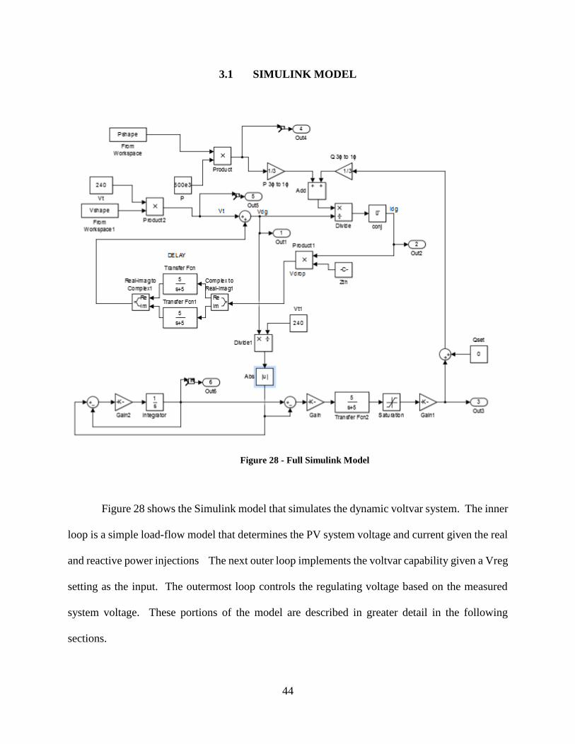
Figure 28 - Full Simulink Model

Figure 28 shows the Simulink model that simulates the dynamic voltvar system. The inner

loop is a simple load-flow model that determines the PV system voltage and current given the real

and reactive power injections The next outer loop implements the voltvar capability given a Vreg

setting as the input. The outermost loop controls the regulating voltage based on the measured

system voltage. These portions of the model are described in greater detail in the following

sections.

45

3.1.1 Load-flow Simulation

The load-flow simulation was constructed as a simple Thévenin equivalent shown in Figure 29

with real and reactive power injections from the PV inverter. Figure 30 shows the Simulink model

block diagram that solves this simple load flow problem.

.

Figure 29 - Simple Thévenin equivalent

46

Figure 30 - Simulink Load Flow solver

In order to simulate a weak grid, the system impedance was chosen such that the short-circuit ratio

was close to 10 (20)-(23). [24] Also, a small X/R ratio (.657) simulates a grid condition where the

required reactive power is high (see Section 1.6.1).

𝑍𝑇 = 0.0134 + 𝑗0.0088 Ω (20)

𝑉𝐿𝐿 = 416 V (21)

𝑃𝑃𝑉 = 600 kW (22)

𝑆𝐶𝑅 =𝑆𝑆𝐶

𝑃𝑃𝑉=

𝑉𝐿𝐿2 /|𝑍𝑇|

𝑃𝑃𝑉= 12.99 (23)

47

The Thévenin voltage (Vshape) rises and falls to simulate the system loading changes throughout

the day. The voltage plot in Figure 31 shows the voltage at the point of common coupling when

the PV system is inactive. This type of voltage fluctuation reflects the typical variation of feeder

loads, capacitor switching, and tap changer steps through the day. The nominal voltage is 240 V,

which is the full split-phase secondary voltage that would serve a residential PV system.

Figure 31 - Voltage at PCC without PV

The selected PV generation curve (Pshape) is plotted in Figure 32 below. This curve

simulated the cloud-induced power output swings that cause voltage fluctuations throughout the

day.

0 5 10 15 20 25225

230

235

240

245

250

255

Time (hr)

Voltage (

V)

ANSI Limit

48

Figure 32 - PV generation curve

The transfer functions that are applied to the voltage feedback provide a delay that serves to prevent

algebraic loops. This delay is unnoticeable during the timescale of interest (~1 minute) and allows

Simulink to iterate to a solution of the load flow problem. Figure 33 shows the point of common

coupling (PCC) voltage in the unity power factor case.

0 5 10 15 20 25-0.2

0

0.2

0.4

0.6

0.8

1

1.2

Time (hr)

Pow

er

(p.u

. ra

ted)

49

Figure 33 - PCC Voltage (Unity PF)

3.1.2 Static volt-var simulation

Figure 34 - Volt-var response in Simulink

0 5 10 15 20 25225

230

235

240

245

250

255

Time (hr)

Voltage (

V)

ANSI Limit

50

The next simulation incorporated a static volt-var capability in which the inverter

attempts to regulate the voltage to 1.01 per-unit. As shown in Figure 34, the error signal is

calculated and multiplied by the droop setting and passed through a delay element. This delay

element prevents an algebraic loop and simulates the dynamics of a volt-var control scheme.

Figure 35 demonstrates this functionality and shows its ability to lessen voltage fluctuations

throughout the day. The Voltage Variability Index (VVI), normalized to the unity power factor

case, was calculated to be 0.82726.

Figure 35 - PCC Voltage with static volt-var implementation

0 5 10 15 20 25225

230

235

240

245

250

255

Time (hr)

Voltage (

V)

ANSI Limit

51

3.1.3 Dynamic Vreg voltvar simulation

Figure 36 - Simulink block diagram showing dynamic Vreg control

Figure 36 shows the additional control loop that was added to the static volt-var inverter. The goal

of the moving regulating voltage (Vreg) setpoint is to adapt to the slower voltage changes in the

system while resisting the shorter-term fluctuations associated with PV. Consequently, the simple

closed-loop transfer function of the voltage-tracking system was chosen such that the regulating

voltage approaches the system voltage at a time constant of 20 minutes. The Figure 37 below

shows the response of the system to a step input (top) and to the measured voltage of the load flow

simulation (bottom).

52

Figure 37 - Vreg tracking to a step-input (top) and load flow (bottom)

This demonstrates the ability of the system to track the local voltage and ensure the inverter

is properly minimizing voltage fluctuations. When the target voltage is approximately in the

middle of the voltage fluctuations, the inverter is less likely to encounter limitations in its rating

that would lead to saturation and a failure to regulate fluctuations. This ability could be particularly

useful when the inverter is only rated slightly higher than its irradiance rating which only allows

the inverter to provide a small amount of reactive power during peak generation time.

0 0.5 1 1.5 2 2.5 3

0

0.5

1

Time (hr)

Voltage (

p.u

.)

VDG

Vreg

0 1 2 3 4 5 6 7 8 9

x 104

0.95

1

1.05

Time (hr)

Voltage (

p.u

.)

VDG

Vreg

53

3.2 ADVANTAGES OF DYNAMIC VOLT-VAR

3.2.1 Improved Performance

Figure 38 shows the performance of the dynamic Vreg system and provides a comparison to the

previously discussed simulations. Incorporating the dynamic Vreg control-loop into the volt-var

inverter reduces the Voltage Variability Index from 0.82726 to 0.73278.

Figure 38 - Voltage PCC using different inverter settings

The control loop could easily be adjusted to support other objectives as needed for

improving the system performance. For example, if minimizing losses is an objective, the control

would be modified to increase system voltage. Such objectives could be accomplished by

54

maintaining a constant difference between Vreg and the measured voltage or through a constant

var offset.

3.2.2 Automatic Setting Selection

The additional control loop alleviates the user from the burden of choosing an appropriate setting.

The system establishes a suitable Vreg for minimizing voltage fluctuations prior to the start of the

PV power output. This capability is necessary for ensuring autonomous control of the inverter

does not cause adverse system impacts due to poorly chosen settings.

3.2.3 Reactive Demand

The reactive power output depends on the operating point of the inverter. If the voltage deviates

a sufficient amount away from Vreg, the inverter will saturate and provide (or absorb) 100% of its

available reactive power. Figure 39 shows a comparison of how much reactive power each control

scheme demands. The static volt-var control scheme operates in its saturation region (full rated

var output) for approximately 20 hours, which is about twice that of the dynamic volt-var control

scheme and puts unnecessary strain on the inverter hardware. The excessive reactive power usage

also increases losses in the inverter and the distribution system, by increasing current when that

isn’t necessary to mitigate the voltage fluctuations.

55

Figure 39 - Comparison of rating usage for static volt-var (left) and dynamic volt-var (right)

56

4.0 CONCLUSION

This thesis provides an overview of the traditional power system and the adverse impacts

of distributed energy resources that lead to the need for more advanced distribution system

modeling. The simulation capabilities of OpenDSS are demonstrated and applied to an actual

feeder in the United States in order to assess the impact of different volt-var settings on distribution

system performance. The relationship between the appropriate settings and the load level, solar

characterization, and performance objectives are observed and discussed. Since the choice of

settings depend on solar and load conditions (thus eliminating the possibility of an “out of the box”

setting), a dynamic volt-var control scheme is proposed. This control scheme shows improved

performance and robustness in setting selection, which alleviates the user of the burden of the

extensive modeling process required for static volt-var setting selection.

For future work, the dynamic volt-var control capability will be incorporated into inverter

models in OpenDSS and applied to the distribution feeder examined in this thesis. Other

capabilities will be explored, such as the ability to maintain a constant voltage or reactive power

offset based on the chosen performance objective. The goal of this future work is to demonstrate

the improvements shown in this thesis on an actual feeder in the United States and validate its

potential for accommodating additional distributed energy resources.

57

BIBLIOGRAPHY

[1] "IEEE Standard for Conformance Test Procedures for Equipment Interconnecting

Distributed Resources with Electric Power Systems -- Amendment 1," ed, 2014.

[2] (December 2014). Solar Industry Data. Available: www.seia.org/research-resources/solar-

industry-data

[3] (March 2015). U.S. Energy Information Administration: Today In Energy. Available:

http://www.eia.gov/todayinenergy/detail.cfm?id=20292

[4] L. C. Dangelmaier, D. Nakafuji, and R. Kaneshiro, "Tools used for handling variable

generation in the Hawaii Electric Light Co. control center," in Power and Energy Society

General Meeting, 2012 IEEE, 2012, pp. 1-8.

[5] EPRI, "EPRI Smart Grid Demonstration Initiative Final Update," 22 October 2014.

[6] C. E. R. 21, "Generating Facility Interconnections," ed, 2014.

[7] M. Rylander, "Integrated Control of Photovoltaic Inverters to Improve Distribution Feeder

Performance," CIGRÉ Canada Conference on Power Systems, September 2014.

[8] (June 2014). Electricity Net Generation: Total (All Sectors). Available:

http://www.eia.gov/totalenergy/data/monthly/pdf/sec7_5.pdf

[9] J. J. Bian, S. Ekisheva, and A. Slone, "Top risks to transmission outages," in PES General

Meeting | Conference & Exposition, 2014 IEEE, 2014, pp. 1-5.

[10] N. H. S. Papathanassiou, "Capacity of Distribution Feeders for Hosting DER," CIGRÉ

Working Group C6.24, June 2014.

[11] M. J. Reno and J. S. Stein, "PV output variability modeling using satellite imagery and

neural networks," in Photovoltaic Specialists Conference (PVSC), Volume 2, 2012 IEEE

38th, 2012, pp. 1-3.

58

[12] T. E. McDermott, "Voltage control and voltage fluctuations in distributed resource

interconnection projects," in Transmission and Distribution Conference and Exposition,

2010 IEEE PES, 2010, pp. 1-4.

[13] T. Short, "Electric power distribution handbook," CRC Press 2004.

[14] M. Rylander, J. Smith, D. Lewis, and S. Steffel, "Voltage impacts from distributed

photovoltaics on two distribution feeders," in Power and Energy Society General Meeting

(PES), 2013 IEEE, 2013, pp. 1-5.

[15] R. C. Dugan and T. E. McDermott, "An open source platform for collaborating on smart

grid research," in Power and Energy Society General Meeting, 2011 IEEE, 2011, pp. 1-7.

[16] T. E. McDermott, "Modeling PV for unbalanced, dynamic and quasistatic distribution

system analysis," in Power and Energy Society General Meeting, 2011 IEEE, 2011, pp. 1-

3.

[17] T. A. Short, D. L. Brooks, and R. F. Arritt, "Green Circuit: Distribution Efficiency Case

Studies," 2011.

[18] R. F. Arritt, R. C. Dugan, D. L. Brooks, T. A. Short, and K. Forsten, "Techniques for

analyzing distribution system efficiency alternatives," in Power & Energy Society General

Meeting, 2009. PES '09. IEEE, 2009, pp. 1-4.

[19] B. Le, C. A. Canizares, and K. Bhattacharya, "Incentive Design for Voltage Optimization

Programs for Industrial Loads," Smart Grid, IEEE Transactions on, vol. PP, pp. 1-1, 2015.

[20] B. Seal, "Common Functions for Smart Inverters, Version 3," February 2014.

[21] EPRI. Distributed PV Monitoring and Feeder Analysis. Available: http://dpv.epri.com

[22] J. Stein, C. Hansen, and M. Reno, "The Variabilty Index: A New and Novel Metric for

Quantifying Irradiance and PV Output Variability," ASES Resource Application Division

Newsletter, April 2012.

[23] C. Trueblood, S. Coley, T. Key, L. Rogers, A. Ellis, C. Hansen, et al., "PV Measures Up

for Fleet Duty : Data from a Tennessee Plant Are Used to Illustrate Metrics That

Characterize Plant Performance," Power and Energy Magazine, IEEE, vol. 11, pp. 33-44,

2013.

[24] N. P. W. Strachan and D. Jovcic, "Stability of a Variable-Speed Permanent Magnet Wind

Generator With Weak AC Grids," Power Delivery, IEEE Transactions on, vol. 25, pp.

2779-2788, 2010.