Ekonomický časopis, 60, 2012, č. 10, s. 1005 – 1023 1005

Modeling a Distribution of Mortgage Credit Losses1

Petr GAPKO* – Martin ŠMÍD**1

Abstract

In our paper, we focus on the credit risk quantification methodology. We

demonstrate that the current regulatory standards for credit risk management

are at least not perfect. Generalizing the well-known KMV model, standing behind

Basel II, we build a model of a loan portfolio involving a dynamics of the com-

mon factor, influencing the borrowers’ assets, which we allow to be non-normal.

We show how the parameters of our model may be estimated by means of past

mortgage delinquency rates. We give statistical evidence that the non-normal

model is much more suitable than the one which assumes the normal distribution

of risk factors. We point out in what way the assumption that risk factors follow

a normal distribution can be dangerous. Especially during volatile periods compa-

rable to the current crisis, the normal-distribution-based methodology can under-

estimate the impact of changes in tail losses caused by underlying risk factors.

Keywords: credit risk, mortgage, delinquency rate, generalized hyperbolic dis-

tribution, normal distribution JEL Classification: G21

Introduction

Minimum standards for credit risk quantification are often prescribed in de-

veloped countries with regulated banking. A system of financial regulation has

been developed and is maintained by European supervisory institutions (Basel

* Petr GAPKO – Institute of Economic Studies, Faculty of Social Sciences, Charles University

in Prague, Opletalova 26, 110 00 Prague, Czech Republic; Institute of Information Theory and Au-

tomation, Academy of Sciences of the Czech Republic, Pod Vodárenskou věží 4, 182 08 Prague 8,

Czech Republic; e-mail: petr.gapko@seznam.cz ** Martin ŠMÍD – Institute of Information Theory and Automation, Academy of Sciences

of the Czech Republic, Pod Vodárenskou věží 4, 182 08 Prague 8, Czech Republic; e-mail:

martinsmid.eu@gmail.com 1 Support from the Czech Science Foundation under grants 402/09/H045 and P402/12/G097

and from Charles University under grant GAUK 46108 is gratefully acknowledged.

1006

Committee on Banking Supervision, Committee of European Banking Supervi-

sors – CEBS) with its standards formalized in the Second Basel Accord (Basel

II, see BIS, 2006) which is implemented into European law by the Capital Re-

quirements Directive (CRD) (European Commission, 2006).

For credit risk, Basel II allows only two possible quantification methods –

a Standardized Approach (STA) and an Internal Rating Based Approach (IRB)

(for more details on these two methods see BIS, 2006). The main difference

between STA and IRB is that while the STA methodology is based on prescribed

parameters, under IRB banks are required to use internal measures for both the

quality of the deal (measured by the counterparty’s probability of default – PD)

and the quality of the deal’s collateral (measured by the deal’s loss given default

– LGD).

The PD is the chance that the counterparty will default (or, in other words,

fail to pay back its liabilities) in the upcoming 12 months. A common definition

of default is that the debtor is delayed in its payments for more than 90 days

(90+ days past due).

The LGD, on the other hand, is the percentage of the size of the defaulted

debt which the bank will actually lose given that the default happens – in prac-

tice, the potential 100% loss decreases by expected recoveries from the default,

i.e., the amount that the creditor expects to be able collect back from the debtor

after the debtor defaults; these recoveries are mainly realized from collateral

sales and bankruptcy proceedings.

It is possible to say that PD and LGD are two major and common measures of

deal quality and basic parameters for credit risk measurement. The PD is usually

obtained either from a scoring model, from a Merton-based distance-to-default

model (e.g., Moody's KMV, mainly used for commercial loans; Merton, 1973

and 1974) or as a long-term stable average of past 90+ delinquencies.2 The mod-

el, presented later in the paper, provides a connection between the scoring mod-

els and those based on past delinquencies. The LGD can generally be understood

as a function of collateral value; however, we view LGD as fixed in the present

paper for simplicity.

Once PDs and LGDs have been obtained, we are able to calculate the ex-

pected loss. The expected loss is the first moment of a loss distribution, i.e.,

a mean measure of the credit risk. The expected loss is a sufficient measure of

credit risk on the long-term horizon. However, in the short-term (e.g., the one-

-year horizon), it is insufficient to be protected only against expected losses be-

cause of the stochasticity of the losses. Thus a bank should look into the right tail

2 Delinquency is often defined as a delay in installment payments, e.g., 90+ delinquencies can

be interpreted as a delay in payments for more than 90 days.

1007

or the distribution of the losses and decide which quantile (probability level) of

the loss should be covered by holding a sufficient amount of capital.

Banks usually cover a quantile level suggested by a rating agency, which,

however, has to be no less than the regulatory level 99.9%. This level may seem

a bit excessive, as it can be interpreted as meaning that banks should cover a loss

which occurs once in a thousand years. The reason for choosing such a conserva-

tive value is the usual absence of data for an exact estimation of the quantiles,

resulting in a large error of the quantiles estimation.

The quantile is usually calculated by Value-at-risk type models, such as

Saunders and Allen (2002), Andersson et al. (2001) or by the IRB approach

which assumes that the credit losses are caused by two normally distributed risk

factors: credit quality of the debtor and a common risk factor for all debtors,

often interpreted as the macroeconomic environment (see Vasicek, 1987).

In this paper, we will introduce a new approach to quantifying credit risk

which can be classed with the Value-at-risk models. Our approach is different

from the IRB method in the choice of the loss distribution. In the general version

of our model, we assume a generally non-normal distribution of the risk factors.

Moreover, we model a dynamics of the common factor (modeling a dynamics of

the factor being necessary especially with respect to the present financial crisis).

In the simpler version of our model, which we later apply to the mortgage data,

we keep the IRB assumption of the normal individual factor (credit quality of

a debtor) while allowing a non-normal common factor; in its general form, how-

ever, our approach allows a non-normal individual factor, too, which could be

useful to measure the credit risk of many types of banking products, e.g., con-

sumer loans, overdraft facilities, commercial loans with a lot of variance in col-

lateral, exposures to sovereign counterparties and governments, etc.

As we said previously, we apply our model to the US nationwide mortgage

portfolio assuming the normal distribution of the individual factor and a generalized

hyperbolic distribution of the common factor. We compare our results to the IRB

approach, showing that the assumption of a normal common factor is inappropriate.

There are several other extensions of Vasicek’s model; however, they mainly

focus on the randomness of LGD. The simplest (and the most natural) enhance-

ment of the Vasicek model incorporating LGD is the one proposed in Frye

(2000), which assumes that LGD is a second risk indicator driving credit losses.

An extension of the Frye model can be found in Pykhtin (2003), who supposes

that the risk factor driving LGD depends on one systemic and two idiosyncratic

factors. Another extension of the Vasicek model can be found in Witzany (2011)

where LGD is assumed to be driven by a specific factor different from the one

driving defaults and by two systemic factors, one common to the defaults and the

1008

other specific to LGD. None of these models allows a non-normal distribution

for the PD systemic factor.

The paper is organized as follows. After the introduction we describe the

usual credit risk quantification methods and Basel II – embedded requirements in

detail. Then we derive our method of measuring credit risk, based on the class of

generalized hyperbolic distributions and Value-at-risk methodology. In the last

part, we focus on the data description and verification of our approach's ability to

capture the credit risk more accurately than the Basel II IRB. Further, we

demonstrate that the class of distributions we use better fits the empirical data

than several distributions that are, alongside the IRB’s standard normal distribu-

tion, commonly used for credit risk quantification. At the end we summarize our

findings and offer recommendations for further research.

1. Credit Risk Measurement Methodology

The Basel II document is organized into three separate pillars. The first pillar

requires banks to quantify credit risk, operational risk, and market risk by

a method approved by the supervisor.3 For credit risk there are two possible

quantification methods: the method STA and the method IRB.4 Both methods are

based on quantification of risk-weighted assets for each individual exposure.

The STA method uses measures defined by the supervisor, i.e., each deal is

assigned a risk-weight based on its characteristics. Risk-weighted assets are ob-

tained by multiplying the assigned risk-weight by the amount that is exposed to

default. The IRB approach, on the other hand, is more advanced than STA. It is

based on a Vasicek-Merton credit risk model (Vasicek, 1987) and calculation of its

risk-weighted assets is more complicated than in the STA case. First of all, PD

and LGD are used to define the riskiness of each deal. These measures are then

used to calculate risk-weighted assets based on the assumption of normal distri-

bution for the asset value. In both cases, the largest permitted loss that could

occur at the 99.9% level of probability5 is stated as 8% of the risk-weighted as-

sets (for more details on calculations of risk-weighted assets see BIS, 2006). The

loss itself is defined as the amount that is really lost when a default occurs. The

default is defined as a delay in payments for more than 90 days (90+ delinquency).

3 A supervisor is a regulator of a certain country’s financial market; for the Czech Republic,

the supervisor is the Czech National Bank. 4 As defined in the provision of the Czech National Bank No. 123/2007 Sb. 5 The 99.9% level of probability is defined by the Basel II document and is assumed to be

a far-enough tail for calculating losses that do not occur with a high probability. Note that a 99.9%

loss at the one-year horizon means that the loss occurs once in 1 000 years on average. Because the

human race lacks such a long dataset, 99.9% was chosen based on rating agencies’ assessments.

1009

1.1. Expected and Unexpected Loss for an Individual Exposure

The expected and unexpected losses are the two basic measures of credit risk.

The expected loss is the mean loss, i.e., the expectation of the loss distribution,

whereas the unexpected loss is the random difference between the expected and

the actual loss. First, let us focus on expected and unexpected loss quantification

for a single exposure, e.g., one particular loan based on PD and LGD. As there is

no PD or LGD feature in the STA method, and because regulatory institutions

are interested only in unexpected losses, under STA it is impossible to calculate

the expected loss, and even the unexpected loss calculation is highly simplified

and based on benchmarks only. On the other hand, the advantage of this method

is its simplicity. The IRB approach uses PDs and LGDs and thus is more accu-

rate than the STA but relatively difficult to maintain.

A bank using the IRB method has to develop its own scoring and rating mod-

els to estimate PDs and LGDs. These parameters are then used to define each

separate exposure.6 The average loss that could occur in the following 12 months

is calculated as follows:

. ( ) . EL PD E LGD EAD (1)

where

EAD – the exposure-at-default,7

EL – the abbreviation for Expected Loss.

The EAD is usually regarded as a random variable as it is a function of

a Credit Conversion Factor – CCF;8 however, for mortgage portfolios, CCF is

prescribed by the regulator as a fixed value. For our calculations we assume that

if a default is observed, it happens on a 100% drawn credit line, so we don’t treat

EAD as a variable but as a constant.

EL can be regarded as an “ordinary” loss that would occur each year and thus

is something that banks incorporate into their loan-pricing models so it has to be

covered by ordinary banking fees and/or interest payments. However, banks also

have to protect themselves against the randomness of the loss, which they do by

holding capital to cover the maximum loss that could occur at the regulatory

6 Exposure is the usual expression for the balance on a separate account that is currently ex-

posed to default. We will adopt this expression and use it in the rest of our paper. 7 Exposure-at-default is a Basel II expression for the amount that is (at the moment of the

calculation) exposed to default. 8 CCF is a measure of what amount of the loan (or a credit line) amount is on average with-

drawn in the case of a default. It is measured in percentage of the overall financed amount and is

important mainly for off-balance sheet items (e.g., credit lines, credit commitments, undrawn part

of the loan, etc.).

1010

probability level at minimum. To capture the variability in credit losses and to

calculate the needed quantile of the loss distribution, we clearly need to know the

shape of the loss distribution.

On the deal level, the distribution of the loss can be easily determined: De-

fault is a binary variable occurring with a probability equal to PD. If the LGD

is positive, the loss occurs with the same probability as the default, and the

distribution of the loss can readily be determined from the distribution of the

LGD.9

1.2. Expected and Unexpected Loss for a Portfolio

On the portfolio level (constructed from a certain number of individual

deals), the expected loss can be calculated easily: since the loss of the portfolio

as a whole is the sum of the losses of individual deals, its expected loss equals,

by the additive property of expectations, to the sum of expressions (1) for all the

individual deals. If, in addition, the PDs of the individual deals are identical and

the LGDs are equally distributed then the expected loss comes out as PD times

the sum of the individual EAD’s. However, the calculation of the unexpected

loss on the portfolio level is not so straightforward for the reason that deals may

be correlated with each other within a complicated correlation structure that is

usually unknown.

There are two ways of constructing a model for calculating unexpected loss.

If the correlation structure among the individual deals is known, we can calcu-

late the variance of the unexpected loss from the variances of individual deals

and the correlation matrix. This approach is often referred to as a bottom-up

one. Often, however, the correlation matrix of the individual deals is not

known and thus a different approach has to be chosen to determine the unex-

pected loss of the loan portfolio. The second approach is widely known as

a top-down approach and the main idea is to estimate the loss distribution

based on historical data or assume a distribution structure and determine the

standard deviation or directly find the difference between the chosen quantile

and the mean value.10

In the present paper, we assume a rather simple dependence structure of the

individual deals, similar to the one from Vasicek (2002): in particular, we

assume that the default happens if a factor variable of a deal, summing an

individual and a common part, falls below a certain threshold.

9 Please note that the LGD variable may take on negative values in some cases. This is, for

example, a situation when a loan’s collateral covers the loan value and a bank collects some addi-

tional cash on penalty fees and interest. 10 Remember that the loss mean value equals the expected loss of a deal.

1011

2. Our Approach 2.1. The Distribution of Loan Portfolio Value

The IRB to modeling the loan portfolio value is based on the famous paper by

Vasicek (2002) assuming that the value ,1iA or the -th's borrower's assets at time

one can be represented as

,1 ,0log logi i iA A X (2)

where

,0iA – the borrower's wealth at time zero,

and – constants,

iX – a (unit normal) random variable, which may be further decomposed as

i iX Y Z

where

– a factor common to all the borrowers,

– a private factor, specific to each borrower.

It is assumed that, at time t – 1, all the borrowers, having the same initial

wealth ,0iA = 0A , take mortgages of the same size. Assuming the number of the

borrowers to be very large and applying the Law of Large Number to the

conditional distribution of the wealth given the common factor , the famous

Vasicek distribution of the percentage loss of the portfolio holder (i.e., the

percentage of those borrowers whose wealth ,1iA at time is not sufficient to

repay that mortgage) is obtained (see Vasicek, 2002 for details).

2.1.1. The Generalization

We generalize the model in two ways: we assume a dynamics of the common

factor over discrete times t = 1, 2… and we allow non-normal distributions of

both the common and private factors. For each time, t we assume, similarly

to the original model, that

, , 1 ,log logi t i t t i tA A Y U (3)

where

– the wealth of the -th borrower at time,

t – a random variable specific to the borrower,

tY – the common factor following a general (adapted) stochastic process with

a deterministic initial value 0Y .

For simplicity, we assume that the duration of the debt is exactly one period

and that different borrowers take mortgages in each period, the initial wealth of

1012

each borrower equating to the (cummulative) common factor plus a zero mean

borrower-specific disturbance, i.e.,

1, 1 1 ,log t

i t j j i tA Y V for all i n where ,i tV is a centered random variable specific to the borower –

such an assumption makes sense, for instance, if tY stands for log-returns of

a stock index which and the borrower owns a portfolio with the same com-

position as the index plus some additional assets.

Suppose ,i tU and ,i tV to have the same distribution with zero mean and with

a strictly increasing cummulative distribution function for each i n , ,t

where n is the number of borrowers and that all , , ,( , )i t i t i n tU V are mutually

independent and independent of ( )t tY . Note that we do not require increments

of tY to be centered (which may be regarded as compensation for the term

present in (1) but missing in (2)). 2.1.2. Percentage Loss (Delinquency Rate) in the Generalized Model

Denote )  (t tY Y the history of the common factor up to time t Analo-

gously to the original model, the conditional probability of the bankruptcy of the

-th borrower at time given   tY equals to

, , , 1 1| | Ψt ti t i t t i t j j t j jA B Y Z logB Y Y b Y

where 1,1 1,1, Z U V – the cummulative distribution function of Z, ,i tB are

the borrower's debts (installments) which we assume to be the same for all the

borrowers and all times, i.e., ,log ,  , ,i tB b t i n for some b. The primary topic of our interest is the percentage loss (delinquency rate) tL

of the entire portfolio of the loans at time t. After taking the same steps as

Vasicek (1991) (with conditional non-normal c.d.f.s instead of the unconditional

normal ones), we get, for a very large portfolio, that

1Ψ , tt j jL b Y t

further implying that

1 1

1Ψ Ψ ( )t t tY L L (4)

and

11Ψ Ψt t tL L Y (5)

the latter formula roughly determines the dynamics of the process of the losses

(delinquency rates), and the former one allows us to do statistical inference on

1013

the common factor based on the time series of the percentage losses (delinquen-

cy rates). To see that the Merton-Vasicek model is a special version of the

generalized model, see the Appendix.

In the particular version of our general model we work with later, we assume

both and to be normally distributed and the common factor to be an

ARCH process

1

2, tt t t tY c Y

where

1 2, – i.i.d. (possibly non-normal) variables,

c – a constant. Since the equation (3) may be rescaled by the inverse standard deviation of Z

without loss of generality, we may assume that Ψ is the standard normal distri-

bution function. As was already mentioned, we assume the distribution of 1 to

be generalized hyperbolic and we use the ML estimation to get its parameters –

see the Appendix for details. In addition to estimation of the parameters, we

compare our choice of the distribution to several other distribution classes.

2.2. The Class of Generalized Hyperbolic Distributions

Our model is based on the class of generalized hyperbolic distributions, first

introduced in Barndorff-Nielsen, Blæsild and Jensen (1985). The advantage of

this distribution class is that it is general enough to describe fat-tailed data. It has

been shown (Eberlein, 2001; Eberlein and Prause, 2002; Eberlein and von

Hammerstein, 2004) that the class of generalized hyperbolic distributions is bet-

ter able to capture the variability in financial data than a normal distribution,

which is used by the IRB approach. Generalized hyperbolic distributions have

been used in an asset (and option) pricing formula (Rejman, Weron and Weron,

1997; Eberlein, 2001; Chorro, Guegan and Ielpo, 2008), for the Value-at-risk

calculation of market risk (Eberlein and Prause, 2002; Eberlein and Keller, 1995;

Hu and Kercheval, 2008) and in the Merton-based distance-to-default model to

estimate PDs in the banking portfolio of commercial customers (e.g., Oezkan,

2002). We will show that the class of generalized hyperbolic distributions can be

used for an approximation of a loss distribution for the retail banking portfolio

with a focus on the mortgage book.

The class of generalized hyperbolic distributions is a special, quite young

class of distributions. It is defined by the following Lebesgue density:

0,5

2 2 2 220,5

; , , , ,

, , , ( ( ) ) ( (( ( ) ))exp(

gh x

a x K x x

(6)

1014

where 2 2 0,5

0,5 2 2

( ), , ,

2 . ( )K

and Kλ is a Bessel function of the third kind (or a modified Bessel function – for

more details on Bessel functions see Abramowitz, 1968). The GH distribution

class is a mean-variance mixture of the normal and generalized inverse Gaussian

(GIG) distributions. Both the normal and GIG distributions are thus subclasses

of generalized hyperbolic distributions. Here µ and δ are scale and location pa-

rameters, respectively. Parameter β is the skewness parameter, and the trans-

formed parameter determines the kurtosis. The last parameter, λ, deter-

mines the distribution subclass. There are several alternative parameterizations

described in the literature using transformed parameters to obtain scale- and

location-invariant parameters. This is a useful feature that will help us with the

allocation of economic capital to individual exposures. For the moment-genera-

ting function and for more details on the class of generalized hyperbolic distribu-

tions, see the Appendix.

Because the class of generalized hyperbolic distributions has historically been

used for different purposes in economics as well as in physics, one can find sev-

eral alternative parameterizations in the literature. In order to avoid any confu-

sion, we list the most common parameterizations. These are:

2 2  , 

0,5  (1 ) ,  

, 

The main reason for using alternative parameterizations is to obtain a location-

and scale-invariant shape of the moment-generating function (see the Appendix).

3. Data and Results

3.1. Data Description

To verify whether or not our model based on the class of generalized hyper-

bolic distributions is able to better describe the behavior of mortgage losses, we

used data from the US mortgage market, namely the a dataset consisting of quar-

terly observations of 90+ delinquency rates on mortgage loans collected by the

US Department of Housing and Urban Development and the Mortgage Bankers

1015

Association.11

This data series is the best substitute for losses that banks faced

from their mortgage portfolios, relaxing the LGD variability (i.e., assuming that

LGD = 100%). The dataset begins with the first quarter of 1979 and ends with

the third quarter of 2009. The development of the US mortgage 90+ delinquency

rate is illustrated in Figure 1. We observe an unprecedentedly huge increase in

the 90+ delinquency rate beginning with the second quarter of 2007.

F i g u r e 1

Development of US 90+ Delinquency Rate

Source: US Department of Housing and Urban Development.

F i g u r e 2

Comparison of the Development of the Common Factor and Lagged S&P 500 Returns

Source: Own calculations (Common factor), finance.yahoo.com (S&P 500).

Starting our analysis, we have computed the values of the common factor Y

using the formula (4) with the standard normal Ψ . Quite interestingly, its evolu-

tion is indeed similar to the one of the US stock market – see Figure 2, displaying

11 The Mortgage Bankers Association is the largest US society representing the US real estate

market, with over 2 400 members (banks, mortgage brokers, mortgage companies, life insurance

companies, etc.).

0

1

2

3

4

5

Q1_

197

9

Q1_

198

0

Q1_

198

1

Q1_

198

2

Q1_

198

3

Q1_

198

4

Q1_

198

5

Q1_

198

6

Q1_

198

7

Q1_

198

8

Q1_

198

9

Q1_

199

0

Q1_

199

1

Q1_

199

2

Q1_

199

3

Q1_

199

4

Q1_

199

5

Q1_

199

6

Q1_

199

7

Q1_

199

8

Q1_

199

9

Q1_

200

0

Q1_

200

1

Q1_

200

2

Q1_

200

3

Q1_

200

4

Q1_

200

5

Q1_

200

6

Q1_

200

7

Q1_

200

8

Q1_

200

9

0

200

400

600

800

1000

1200

1400

1600

1800

0

0,5

1

1,5

2

2,5

12

-79

1-8

1

2-8

2

3-8

3

4-8

4

5-8

5

6-8

6

7-8

7

8-8

8

9-8

9

10

-90

11

-91

12

-92

1-9

4

2-9

5

3-9

6

4-9

7

5-9

8

6-9

9

7-0

0

8-0

1

9-0

2

10

-03

11

-04

12

-05

1-0

7

2-0

8

3-0

9

Common Factor

S&P 500

1016

the common factor (left axis), adjusted for inflation, against the S&P 500 stock

index. The correlation analysis indicates that the common factor lags behind

the index by two quarters (the value of the Pearson correlation coefficient is

about 30%).

3.2. Results

We considered several distributions for describing the distribution of 1

(hence of 1( )t tL after a transform), namely loglogistic, logistic, lognormal,

Pearson, inverse Gaussian, normal, lognormal, gamma, extreme value, beta and

the class of generalized hyperbolic distributions.

In the set of the distributions compared, we were particularly interested in the

goodness-of-fit of the class of generalized hyperbolic distributions and their

comparison to other distributions. In particular, after estimating c whose estimate

is independent of the distribution of 1 , we have, for each compared distribution,

fitted its parameters using the maximum likelihood (see the Appendix for the

proof that this procedure is correct) and computed the chi-square goodness-of-fit

statistics:

2 2

1

( ) /k

i i i

i

O E E (8)

where

Oi – the observed frequency in the i-th bin,

Ei – the frequency implied by the tested distribution,

k – the number of bins.

It is well known that the test statistic asymptotically follows the chi-square

distribution with (k – c) degrees of freedom, where c is the number of estimated

parameters. In general, only the generalized hyperbolic distribution from all con-

sidered distributions was not rejected to describe the dataset on a 99% level (the

statistic value was 22.59 with a p-value 0.0202).

Figure 1 graphically shows the difference between the estimated generalized

hyperbolic and normal distributions. From Figure 1 we can see that the GHD is

better able to describe both the skewness and the kurtosis of the dataset.

The main result of our estimation is that the class of generalized hyperbolic

distributions is the only one suitable to describe the behavior of delinquencies

among a wide variety of alternatives. The main reason for this is, in our opinion,

the fact that GHD are fat-tailed, which suggests a need for a larger stock of capi-

tal to cover a certain percentile delinquency. We demonstrate this in the next

Section.

1017

F i g u r e 3

Compared Histograms: GHD vs. Normal vs. Dataset

Source: Own calculations.

3.3. Economic Capital at the One-year Horizon: Implications for the Crisis

The IRB formula, defined in Pillar 1 of the Basel II Accord, assumes that

losses follow a distribution that is a mix of two standard normal distributions

describing the development of risk factors and their correlation. The mixed dis-

tribution is heavy-tailed and the factor determining how heavy the tails are is the

correlation between the two risk factors. However, because the common factor is

considered to have the standard normal distribution, the final loss distribution’s tails

may not be heavy enough. If a heavy-tailed distribution is considered for the com-

mon factor, the final loss distribution will probably have much heavier tails. Because

the regulatory capital requirement is calculated at the 99.9% probability level, this

may lead to serious errors in the assessment of capital needs. To show the differ-

ence between the regulatory capital requirement (calculated by the IRB method)

and the economic capital requirement calculated by our model, we performed the

economic capital requirement calculations at the 99.9% probability level as well.

When constructing loss forecasts, we repeatedly used (5) to get

1

4 1

1 4

Ψ( )Ψ ( )t t t

i

L L Y

(note that our data were quarterly and that a one-year forecast is required). If we

wanted to describe the distribution of the forecasted values exactly, we would

face complicated integral expressions. We therefore decided to use simulations to

obtain annual figures. We were particularly interested in the capital requirement

based on average loss and the capital requirement based on last experienced loss.

Histogram of Data

Data

Den

sity

1018

The average loss was calculated as the mean value from the original dataset of 90+

delinquencies and served as a through-the-cycle PD estimate. This value is impor-

tant for the regulatory-based model (Basel II), as a through-the-cycle PD should be

used there. The last experienced loss is, on the other hand, important for our model

due to the dynamical nature of the model. The Table 1 summarizes our findings.

To illustrate how our dynamic model would predict if the normal distribution of

the common factor was used, we added this version of the dynamic model as well.

T a b l e 1

Comparison of Basel II, Dynamic Normal and Dynamic GHD Models Tail

Delinquency Rates

Model Basel II IRB

(through-the-cycle PD)

Our dynamic model

with normal

distribution

Our dynamic model

with GHD

Distribution used for the individual factor

Standard Normal Standard Normal Standard Normal

Distribution used for

the common factor

Standard Normal Normal Generalized Hyperbolic

99.9% loss 10.2851% 9.5302% 12.5040%

Source: Own calculations.

The first column in Table 1 relates to the IRB Basel II model, i.e., a model

with a standard normal distribution describing the behavior of both risk factors

and the correlation between these factors set to the usual value of 15%. The PD

used in the IRB formula (see Vasicek, 2002 for details) was obtained from the

original dataset as an average default rate through the whole time period. The

second column contains results from the dynamic model with a normal individu-

al common factor. The last column is related to our dynamic model with the

GHD of the common factor (for estimated parameter values, see the Appendix).

The results in Table 1 show that the dynamic model, based on the last experi-

enced loss, predicts higher quantile losses in the case of GHD and slightly lower

in the case of a normal distribution, compared to the IRB formula. Thus, heavy

tails of the GHD distribution evoke higher quantile losses than the current regu-

latory IRB formula, which ultimately leads to a higher capital requirement.

Conclusion

We have introduced a new model for quantification of credit losses. The mo-

del is a generalization of the current framework developed by Vasicek and our

main contribution lies in two main attributes: first, our model brings dynamics

into the original framework and second, our model is generalized in the sense that

any probability distribution can be used to describe the behavior of risk factors.

1019

To illustrate that our model is better able to describe past risk factor behavior

and thus better predicts the future need for capital, we compared the performance

of several distributions common in credit risk quantification. In this sense, we

were particularly interested in the performance of the class of Generalized Hy-

perbolic distributions, which is often used to describe heavy-tail financial data.

For this purpose, we used a quarterly dataset of mortgage delinquency rates from

the US financial market. Our suggested class of Generalized Hyperbolic distribu-

tions showed much better performance.

We have compared our dynamic model with the current risk measurement

system required by the regulations. Our results show that the mix of standard

normal distributions used in the Basel II regulatory framework underestimates

the potential unexpected loss on the one-year horizon. Therefore, introducing the

dynamics with a heavy-tailed distribution describing the common factor may

lead to a better capturing of tail losses.

Despite the good results of our model, there are still several questions that

need to be answered before our model (with the class of generalized hyperbolic

distributions as a noise in the process of the common factor) can be used for

credit risk assessment. First question points at the use of the 99.9th quantile. As

this was chosen by the Basel II framework based on benchmarks from rating

agencies, it is not known whether this particular quantile should be required in

our dynamic generalized model. Second, more empirical studies have to be per-

formed to prove the goodness-of-fit of the class of generalized hyperbolic distri-

butions. The final suggestion is to add an LGD feature to the calculation to ob-

tain a general credit risk model.

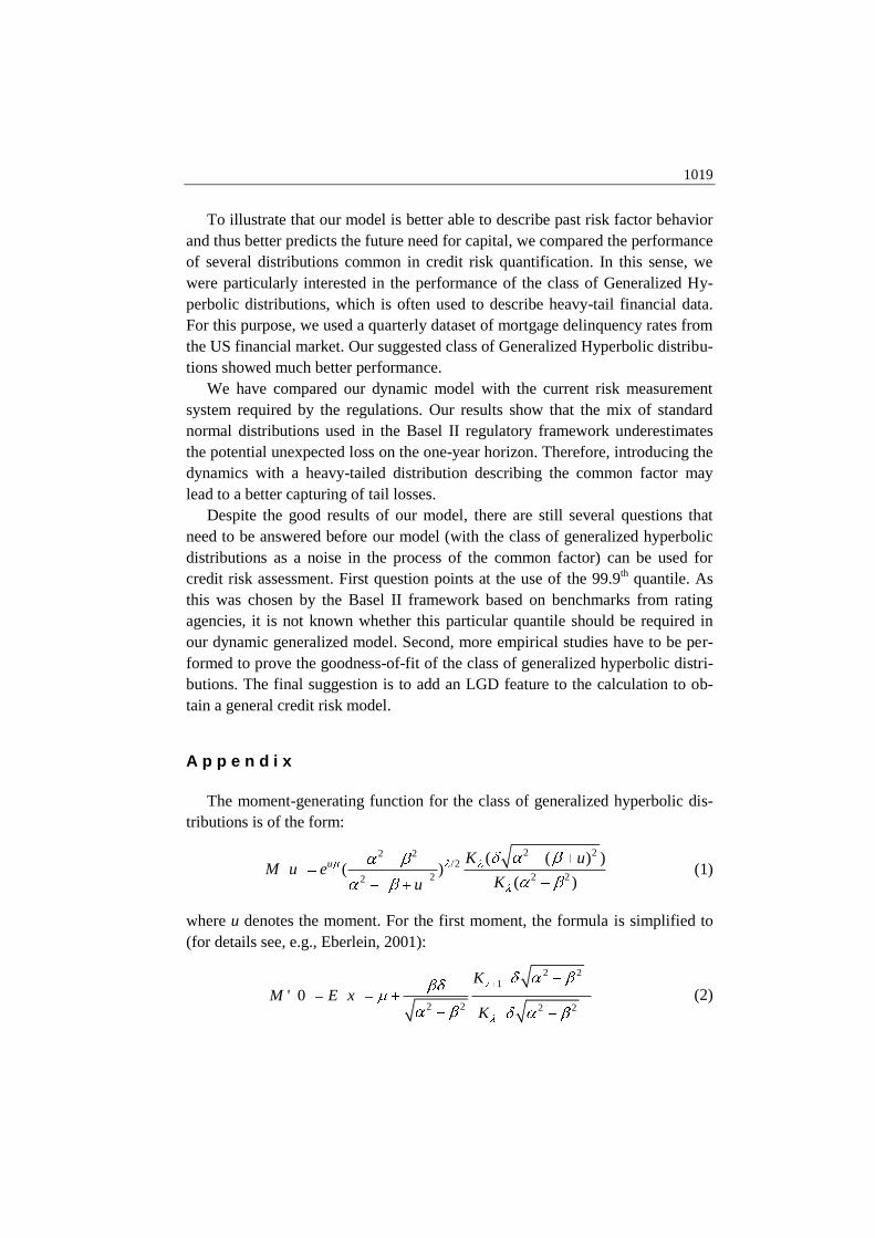
A p p e n d i x

The moment-generating function for the class of generalized hyperbolic dis-

tributions is of the form:

2 22 2/2

2 2 22

( ( ) )  ( )

( )

u K uM u e

Ku (1)

where u denotes the moment. For the first moment, the formula is simplified to

(for details see, e.g., Eberlein, 2001):

2 21

2 2 2 2' 0

KM E x

K (2)

1020

The second moment is calculated in a (technically) more difficult way:

2 21

2

2 2 2 2

22 2 2 22

2 1

2 2 2 2 2 2

'' 0K

M Var xK

K K

K K

(3)

By substituting from equations (2) and (3) into equation (1) we obtain a much

simpler expression for the first and second moments of the class of generalized

hyperbolic distributions. The following equations express the first and the sec-

ond moment of the class of generalized hyperbolic distributions in their scale-

and location-invariant shape:

1

2 21

KM E x

K

22

1 2 12

2 2  2

K K KM Var x

K K K

On MLE Estimation of the Parameters

To estimate the parameters of the model, i.e., the constant c and the vector of

parameters of (the distribution of) 1 , we apply the (quasi) ML estimate to the

sample 2 3, Y Y computed from (4), using the fact that the conditional density

of tY given 1tY is

; . ( ) ; t tf y c c y 1

2 21( )t tc Y c

where ;Θz is the p.d.f. of the distribution 1 dependent on parameters . The

(quasi) log-likelihood function is then

2 2

.Θ log( ( )) log( ;  ΘT T

t t i

i i

L c c c Y

Therefore, if the distribution of 1 has a free scaling parameter which is part

of , we may find its maximum in two steps: first, estimate the value of by

maximizing the left-hand sum, and, second, find the parameter by a maximiza-

tion of the right hand sum which is, incidentaly, the likelihood function of the

1021

distribution of 1 so the standard ML procedure may be used to maximize it (the

existence of the scaling parameter guarantees independence of the right sum’s

minimum on ).

The Merton-Vasicek Model as a Special Case of Our Generalized Framework

In the current section, we show how our generalized model relates to the

original one. Let us start with the computation of the loss's distribution. Reall

that, in our model, the probability of default equals

1, , 1 1 1 1( | )  ( | ) ( )t t

t i t i t t t j j t t j jp A B Y b Y Y b Y

where 1,: t t tY Z , t is its conditional c.d.f. given 1tY and t is the

conditional c.d.f. of tY . Further, by section III.2,

11 1 1

1 1 1

1 1t

( | ) (Ψ | )

(Ψ ( ) ) ( ( ) Ψ ( ))

1 Φ Ψ

tt t j j t

t t t t

t

L Y b Y Y

p Y Y p

p

recall that Ψ the c.d.f. of 1,tZ . Further, denoting , ,: i t t i tX Y Z , we get

, , 1 , 1 1cov( , ) var( , ) var( )i t j t t i t t t tX X Y X Y Y Y

and, consequently,

1

, , 1

1

var( )( , )

var( ) var( )

t t

i t j t t

t t t

Y Ycorr X X Y

Y Y Z

Now, if we assume, with Vasicek (2002), that

1 1,1: (0, ),   : (0, 1 )Y N Z N

for a certain then clearly 1 : (0, 1)N implying

1 11

1

1 11

( ) 1 ( )( ) 1

1 ( ) ( )

N p NL N

N N pN

and

,1 ,1( , )i jcorr X X

i.e., the formulas of Vasicek (2002).

1022

Estimated parameters of the GHD distribution:

lambda alpha mu sigma gamma

0.0995296201 0.5711172510 –0.0005942671 0.0234327245 0.0081063782

log-likelihood:

292.9479

AIC

–575.8958

Parameter variance covariance matrix

lambda alpha mu sigma gamma

lambda 1.3666785019 –0.3367366178 –6.805791e–04 –1.974175e-02 6.803657e-04 alpha –0.3367366178 0.3816490666 –5.602050e–04 –2.925449e-02 4.998918e-04 mu –0.0006805791 –0.0005602050 9.634706e–06 1.405187e-04 –9.641320e-06 sigma –0.0197417490 –0.0292544924 1.405187e–04 1.285614e-02 –9.736328e-05 gamma 0.0006803657 0.0004998918 –9.641320e–06 –9.736328e-05 1.481876e-05

Source: Own calculations.

Referencees ABRAMOWITZ, S. (1968): Handbook of Mathematical Functions. New York: Dover publishing.

ANDERSSON, F. – MAUSSER, H. – ROSEN, D. – URYASEV, S. (2001): Credit Risk Optimiza-

tion with Conditional Value-at-risk Criterion. Mathematical Programming, 89, No. 2, pp. 273 –

291.

BIS (2006): Basel II: International Convergence of Capital Measurement and Capital Standards:

A Revised Framework. Basel: Bank for International Settlements. Retrieved from: <http://

www.bis.org/publ/bcbs128.htm>.

BARNDORFF-NIELSEN, O. E. – BLÆSILD, P. – JENSEN, J. L. (1985): The Fascination of

Sand. A Celebration of Statistics. New York: Springer Verlag, pp. 57 – 87.

CHORRO, C. – GUEGAN, D. – IELPO, F. (2008): Option Pricing under GARCH Models with

Generalized Hyperbolic Innovations (II): Data and Results. Paris: Sorbonne University.

EBERLEIN, E. (2001): Application of Generalized Hyperbolic Lévy Motions to Finance. Lévy

Processes: Theory and Applications. Boston: Birkhäuser, pp. 319 – 337.

EBERLEIN, E. – PRAUSE, K. (2002): The Generalized Hyperbolic Model: Financial Derivatives

and Risk Measures. In: GEMAN, H., MADAN, D., PLISKA, S. and VORST T. (eds): Mathe-

matical Finance-Bachelier Congress 2000. Heidelberg: Springer Verlag, pp. 245 – 267.

EBERLEIN, E. – von HAMMERSTEIN, E. A. (2004): Generalized Hyperbolic and Inverse

Gaussian Distributions: Limiting Cases and Approximation of Processes. In: DALANG, R.C.,

DOZZI, M. and RUSSO, F. (eds): Seminar on Stochastic Analysis, Random Fields and Appli-

cations IV. Progress in Probability, Vol. 58. Basel: Birkhäuser, pp. 221 – 264.

EBERLEIN, E. – KELLER, U. (1995): Hyperbolic Distributions in Finance. Bernoulli, 1, No. 3,

pp. 281 – 299.

EC (2006): Directive 2006/49/EC of the European Parliament and of the Council of 14 June 2006.

Brussels: European Commission.

FRYE, J. (2000): Collateral Damage. Risk, 13, April, pp. 91 – 94.

HU, W. – KERCHEVAL, A. (2008): Risk Management with Generalized Hyperbolic Distribu-

tions. Tallahassee: Florida State University.

MERTON, R. C. (1974): On the Pricing of Corporate Debt: The Risk Structure of Interest Rates.

Journal of Finance, 29, No. 2, pp. 449 – 470.

1023

MERTON, R. C. (1973): Theory of Rational Option Pricing. Bell Journal of Economics and Man-

agement Science, 4, No. 1, pp. 141 – 183.

MOODY's. (n.d.): Moody's KMV. Retrieved from: <www.moodyskmv.com>.

OEZKAN, F. (2002): Lévy Processes in Credit Risk and Market Models. [Dissertation.] Freiburg:

University of Freiburg.

PYKHTIN, M. V. (2003): Unexpected Recovery Risk. Risk, 16, No. 8, pp. 74 – 78.

REJMAN, A. – WERON, A. – WERON, R. (1997): Option Pricing Proposals under the General-

ized Hyperbolic Model. Stochastic Models, 13, No. 4, pp. 867 – 885.

SAUNDERS, A. – ALLEN, L. (2002): Credit Risk Measurement: New Approaches to Value at

Risk and Other Paradigms. New York: John Wiley and Sons.

VASICEK, O. A. (1987): Probability of Loss on Loan Portfolio. [Working Paper.] KMV Corporation.

VASICEK, O. A. (1991): Limiting Loan Loss Probability Distribution. KMV Corporation.

VASICEK, O. A. (2002): The Distribution of Loan Portfolio Value. Risk, 15, December, pp. 160 –

162.

WITZANY, J. (2011): A Two-Factor Model for PD and LGD Correlation. Bulletin of the Czech

Econometric Society, 18, No. 28.