distribution of bed material in a horizontal circulating fluidised bed boiler

Distribution of bed material in a Horizontal Circulating Fluidised Bed boiler An experimental study on a cold model and an industrial boiler Master’s Thesis within the Sustainable Energy Systems programme

THOMAS EKVALL ROBIN MAGNUSSON Department of Energy and Environment Division of Energy Technology CHALMERS UNIVERSITY OF TECHNOLOGY Gothenburg, Sweden 2011 T2011-356

MASTER’S THESIS

Distribution of bed material in a Horizontal Circulating Fluidised Bed boiler

An experimental study on a cold model and an industrial boiler

Master’s Thesis within the Sustainable Energy Systems programme

THOMAS EKVALL

ROBIN MAGNUSSON

SUPERVISOR:

Prof. Yanguo Zhang

Dr. Dongmei Zhao

EXAMINER

Assoc. Prof. Lars-Erik Åmand

Department of Energy and Environment Division of Energy Technology

CHALMERS UNIVERSITY OF TECHNOLOGY Gothenburg, Sweden

Distribution of bed material in a Horizontal Circulating Fluidised Bed boiler An experimental study on a cold model and an industrial boiler Master’s Thesis within the Sustainable Energy Systems programme THOMAS EKVALL ROBIN MAGNUSSON © THOMAS EKVALL, ROBIN MAGNUSSON, 2011 Department of Energy and Environment Division Energy Technology Chalmers University of Technology SE-412 96 Gothenburg Sweden Telephone: + 46 (0)31-772 1000

Cover: Photo of cold horizontal circulating fluidised bed model during operation. Chalmers Reproservice Gothenburg, Sweden 2011

I

Distribution of bed material in a Horizontal Circulating Fluidised Bed boiler

An experimental study on a cold model and an industrial boiler Master’s Thesis in the Sustainable Energy Systems programme THOMAS EKVALL, ROBIN MAGNUSSON Department of Energy and Environment Division of Energy Technology Chalmers University of Technology

ABSTRACT

A conventional circulating fluidised bed (CFB) boiler has a limitation due to the height of the furnace, when implemented in smaller industrial facilities. The design of a horizontal circulating fluidised bed (HCFB) boiler is an interesting approach to resolve this problem. Enabling the benefits, such as high efficiency and fuel flexibility, of the CFB technology for the use in smaller industrial facilities decreases the carbon dioxide emissions tremendously, especially in a country like China.

The purpose of this work is to investigate how a HCFB boiler responds to change in fluidisation velocity and bed mass respectively. The tests are mainly performed using a cold HCFB model and are complemented with tests on an industrial HCFB boiler. The industrial boiler is located at Kings Paper in Xiamen, China, supplying steam to the paper machine.

The result from the cold HCFB model shows an uneven distribution of bed material over the cross sectional area in the 2nd chamber. The distribution of the bed material affect the heat transfer to the tubing walls within the boiler. Uneven distribution of particles will not result in a highest possible heat transfer, thus will affect the efficiency of the boiler.

By making a comparison to the classical CFB, this work shows that the cyclone load is much lower in a HCFB. The cyclone load is an important parameter concerning investment costs. The classical CFB design in this report is represented by the CFB boiler located at Chalmers University of Technology, Gothenburg, Sweden.

Keywords: Circulating fluidised bed; Cold model; Horizontal circulating fluidised bed; Fractionation; Particle distribution

II

Partikelfördelning i en Horisontell cirkulerande fluidiserad bädd Experimentell studie av kallmodell och industripanna Examensarbete inom mastersprogrammet Sustainable Energy Systems THOMAS EKVALL, ROBIN MAGNUSSON Institutionen för Energi och Miljö Avdelningen för Energiteknik Chalmers tekniska högskola

SAMMANFATTNING

Det kan vara svårt att anpassa en cirkulerande fluidiserad bädd (CFB) panna till mindre industrier på grund av det höga pannhuset. Den nya så kallade horisontella cirkulerande fluidiserad bädd (HCFB) pannan är designad för att lösa detta problem. Detta skulle göra det möjligt att nyttja CFB teknikens fördelar, så som hög verkningsgrad och bränsleflexibilitet, även för mindre industrianläggningar. I ett land som Kina kan detta minska de inhemska utsläppen av koldioxid avsevärt.

Syftet med arbetet som presenteras är att se hur flödet i en HCFB svarar på ändringar i fluidiseringshastighet och bäddmassa. Försöken är till största del utförda på en kall HCFB modell och är kompletterade med resultat från en industriell HCFB panna. Den industriella pannan används för att förse en pappersmaskin vid Kings Paper, Xiamen, Kina, med ånga.

Resultatet från den kalla HCFB modellen visar att partiklarna i den andra kammaren inte är jämnt fördelade över tvärsnittet. Fördelningen av bäddmaterialet kommer påverka värmeöverföringen till tubväggarna inne i pannan. En ojämn fördelning innebär att värmeöverföringen inte utnyttjas optimalt, vilket vore önskvärt.

Belastningen på cyklonen är en viktig parameter när det kommer till investerings-kostnader. Genom att göra en jämförelse med en klassisk CFB panna visar resultatet att cyklonbelastningen är lägre i en HCFB panna. Den klassiska CFB designen är i detta arbete representerad av pannan vid Chalmers tekniska högskola i Göteborg, Sverige.

Nyckelord: Cirkulerande fluidiserad bädd; Horisontell cirkulerande fluidiserad bädd; Fraktionering; Kallmodell; Partikelfördelning

III

Table of contents PREFACE ........................................................................................................................................ V NOTATIONS ................................................................................................................................ VII 1 INTRODUCTION ................................................................................................................... 1

1.1 OBJECTIVE ............................................................................................................................ 1 1.2 SCOPE ................................................................................................................................... 1 1.3 METHOD ............................................................................................................................... 1 1.4 BACKGROUND ....................................................................................................................... 2

1.4.1 Fluidised bed boilers .................................................................................................... 2 1.4.2 Scale models at ambient conditions .............................................................................. 3

2 THEORY ................................................................................................................................. 5 2.1 FLUIDISATION ........................................................................................................................ 5 2.2 CIRCULATING FLUIDISED BED BOILER ..................................................................................... 5 2.3 SCALING LAWS ...................................................................................................................... 6

2.3.1 Glicksman’s scaling laws ............................................................................................. 6 2.4 GELDART’S POWDER CLASSIFICATION..................................................................................... 8

3 EXPERIMENTAL SETUP AND PROCEDURE ................................................................... 9 3.1 COLD HCFB MODEL .............................................................................................................. 9 3.2 INDUSTRIAL HCFB BOILER .................................................................................................. 12 3.3 RUNNING CONDITIONS ......................................................................................................... 12 3.4 PREPARATIONS .................................................................................................................... 15

3.4.1 Calibration of pressure sensors .................................................................................. 15 3.4.2 Preparations for the cold HCFB model....................................................................... 15

3.5 MEASUREMENTS .................................................................................................................. 16 3.5.1 Preparations for the industrial HCFB boiler............................................................... 16 3.5.2 Measurements in the cold HCFB model ...................................................................... 16 3.5.3 Measurements at the industrial HCFB boiler .............................................................. 16

3.6 USE OF DATA ....................................................................................................................... 17 4 RESULTS .............................................................................................................................. 21

4.1 BOTTOM BED HEIGHT ........................................................................................................... 21 4.2 RECIRCULATION FLUX OF BED MATERIAL .............................................................................. 21

4.2.1 External recirculation ................................................................................................ 22 4.2.2 Internal recirculation ................................................................................................. 23 4.2.3 Comparison between internal and external recirculation ............................................ 23

4.3 PRESSURE MEASUREMENTS .................................................................................................. 24 4.3.1 Influence of bed mass ................................................................................................. 24 4.3.2 Influence of fluidisation velocity ................................................................................. 25 4.3.3 Effects from external recirculation flow ...................................................................... 26 4.3.4 Pressure measurement in the 2nd chamber .................................................................. 28 4.3.5 Industrial HCFB boiler .............................................................................................. 29 4.3.6 Comparison between the HCFB boiler and the classical CFB boiler ........................... 31 4.3.7 Reference measurements ............................................................................................ 31 4.3.8 Verification measurements ......................................................................................... 33

4.4 CONCENTRATION OF BED MATERIAL ..................................................................................... 33 4.4.1 Influence of bed mass ................................................................................................. 33 4.4.2 Influence of fluidisation velocity ................................................................................. 35 4.4.3 Industrial HCFB boiler .............................................................................................. 36 4.4.4 Comparison between the HCFB boiler and the classical CFB boiler ........................... 37 4.4.5 Cyclone load .............................................................................................................. 38

4.5 PARTICLE SIZE DISTRIBUTION AND FRACTIONATION .............................................................. 38 4.5.1 Cold HCFB model ...................................................................................................... 39 4.5.2 Industrial HCFB boiler .............................................................................................. 41 4.5.3 Comparison between the HCFB boiler and the classical CFB boiler ........................... 44

4.6 VISUAL OBSERVATIONS ........................................................................................................ 46

IV

5 DISCUSSION ........................................................................................................................ 49 5.1 COLD HCFB MODEL ............................................................................................................ 49

5.1.1 Scaling ....................................................................................................................... 49 5.1.2 Bottom bed ................................................................................................................. 50 5.1.3 Recirculation ............................................................................................................. 50 5.1.4 Pressure measurements and concentration of bed material ......................................... 51 5.1.5 Particle size distribution and fractionation ................................................................. 53 5.1.6 Effects from external recirculation flow ...................................................................... 54

5.2 INDUSTRIAL HCFB BOILER .................................................................................................. 54 5.2.1 Pressure measurements and concentration of bed material ......................................... 55 5.2.2 Particle size distribution and fractionation ................................................................. 55

5.3 COMPARISON BETWEEN THE HCFB BOILER AND THE CLASSICAL CFB BOILER ....................... 56 5.3.1 Recirculation ............................................................................................................. 56 5.3.2 Pressure measurements and concentration of bed material ......................................... 57 5.3.3 Particle size distribution and fractionation ................................................................. 58 5.3.4 Cyclone load .............................................................................................................. 58

6 CONCLUSIONS .................................................................................................................... 59 REFERENCES ............................................................................................................................... 61

APPENDIX A – DRAWINGS APPENDIX B – PRESSURE TAPS

APPENDIX C – PRESSURE SENSORS

V

Preface In this study, experiments on a cold model and an industrial boiler have been performed. The results are given here and findings are presented in the conclusions. This study is carried out as a master thesis work within the Department of Energy and Environment at Chalmers University of Technology, Gothenburg. It is also a part of a student exchange program between Chalmers University of Technology and Tsinghua University, Beijing, China. Through this cooperation the tests on the industrial boiler could be carried at a Paper mill in the city of Xiamen and the tests on the cold model could be carried out at Tsinghua University, Beijing. The project lasted for six months from January to June 2011 of which four months were carried out in China and two in Sweden.

The master thesis work is performed by Thomas Ekvall and Robin Magnusson and supervised by Dr. Dongmei Zhao and Prof. Yanguo Zhang. Examiner is Assoc. Prof. Lars-Erik Åmand. Thanks to the helpful operators, Zhong Donghuan et al., of the industrial HCFB boiler in Xiamen that made it possible to perform our measurements. Also thanks to the technicians, Yu Aijun et al., at the laboratory where the cold model was located, for their support and advice.

Finally, thanks to Assoc. Prof. Qinghai Li for valuable discussions and feedback. Also thanks to Heng Feng, Yanqiu Long and Rongrong Cai for technical support and interpretation.

Gothenburg 2011

Thomas Ekvall & Robin Magnusson

VII

Notations Roman letters 퐴 area [m2] 퐴푟 Archimedes number [-] 퐶 constant [-] 퐶 drag coefficient [-] 푑 surface mean particle diameter [m] 퐹 drag force [N] 퐹 gravitational force [N] 퐺 solids flux [kg/m2 s] 푔 acceleration due to gravity [m/s2] 퐻 height [m] 푘 pressure / voltage factor [Pa/V] 퐿 characteristic length [m] 퐿 cyclone load [kg/s] 푚 pressure constant [Pa] 푃 pressure [Pa] 푃 local average pressure for particles [Pa] 푅푒 Reynolds number [-] U voltage signal [V] 푢 velocity [m/s] 푉 volume [m3]

Greek letters 훽 drag coefficient [-] 휌 density [kg/m3] 휌 particle concentration [kg/m3] 휏 time [s] 휇 gas viscosity [Pa s] 휇 particle viscosity [Pa s] 휑 sphericity [-]

Index 0 superficial 1 1st chamber 2 2nd chamber 3 3rd chamber 푏푚 bed mass 푒푥푡 external 푓 fluid 푖푛푡 internal 푚푎푥 maximum 푚푓 minimum fluidisation 푛 sensor number 푠 solid 푝 particle 푤 water

1

1 Introduction As a result of the rapid economic development, the energy demand is high in China. However the use of old inefficient boilers is also high, especially in small industrial facilities. An increase in efficiency of these boilers will reduce the fuel consumption, including coal, sub-stantially. Hence, also reduce the carbon dioxide emissions. Circulating fluidised bed (CFB) boilers have a high efficiency, good emission control and high fuel flexibility. The purpose of developing the horizontal circulating fluidised bed (HCFB) boiler is to enable, to a larger extent, the benefits of CFB technology for the use in small scale industrial facilities.

1.1 Objective The differences in the design of a HCFB boiler yield some differences in the fluid dynamics compared to the classical CFB boiler. The HCFB boiler is relatively new, and there are not so much research material published in the area. The purpose of this thesis work is to examine how the distribution and fractionation of the bed material varies with respect to changes in fluidisation velocity and bed mass in a HCFB.

1.2 Scope Distribution of the bed material in a HCFB is investigated. Two parameters are changed; fluidising velocity and bed mass, while other parameters, such as particle size and temperature, are kept constant. The average concentration over a cross-sectional area is measured and local deviations are only observed visually.

The cold model used, represents the design of HCFB boilers in general but is not a perfectly scaled model from any existing boiler. No combustion take place in the model and it runs at ambient condition. Results and conclusions should be seen as guide lines on a general basis. Estimations of cyclone load and recirculation flux are performed based on measurement of recirculation flow and compared to a classical CFB. Fractionation of the bed material in the cold HCFB model is compared to fractionation of bed material in an industrial HCFB boiler and a classical CFB boiler.

1.3 Method A cold model is used to study the distribution of bed material and the fluid dynamics in a horizontal circulating fluidised bed boiler. By using a cold model the influence of changing fluidising velocity and bed mass on the fluid dynamics can be isolated from the influence of combustion. Also a model is cheaper to construct, easier to handle and render more measurement opportunities than a full scale boiler. Experiments on an industrial HCFB boiler are performed in order to make a comparison to the results from the cold model. Also in this boiler, the influence of changing fluidising velocity and bed mass on the boiler performance was studied.

When varying the fluidisation velocity and bed mass the concentration and fractionation of the bed material together with the pressure drop and recirculation flow in the cold model are measured. Pressure sensors, laser diffraction system, density analyser and mechanical sieves are used to obtain the data from the cold HCFB model and the industrial HCFB boiler.

The results from the cold model are, when feasible, compared to results from similar tests at a classical CFB boiler located at Chalmers University of Technology in Gothenburg, Sweden.

2

1.4 Background The energy consumption in China is increasing rapidly, as the economy strengthens. Of this consumption, 70% is produced from coal (Li et al., 2011). The growth of the economy and the energy consumption is so fast that the auxiliary facilities have no time to update in order to cope with. Therefore there are still many old boilers for industrial applications in use, with an operating efficiency of typically 60-65 %. As a comparison, the efficiency of the same kind of boilers is over 80% in most of the developed countries (UNEP 2001). China consumed 2.7 billion tonnes of coal in 2008 (IEA) and is also the world’s largest emitter of sulphur dioxide (Li et al., 2011).

1.4.1 Fluidised bed boilers Fluidised beds have been used for many applications for a long time e.g. combustion of solid fuels. The first boilers based on fluidisation were of the type of bubbling fluidised bed, BFB (Grace, et al., 1997). One of the advantages of a fluidised bed boiler compared to a Pulverised coal boiler or a Grate fired boiler is the possibility to use every type of solid fuel, in every possible combination, as long as the heating value is sufficient to sustain the combustion process (Li et al., 2009) (Johansson et al.,2006). This flexibility makes it possible to adjust the choice of fuel depending on the market supply and also to co-combust different fuels in order to reduce the use of fossil fuels. It is not only biomass that can be combusted in order to reduce the environmental impact but also waste (Basu et al., 2000). Another advantage is the possibility to add lime stone to the bed material resulting in a reduction of sulphur emissions (Kullendorff, Leckner, 1991). The cooling surfaces in the bed of a BFB boiler tend to be insufficient when the heating value is too high, e.g. if coal is combusted. This can be solved by increasing the fluidisation velocity. Due to the increased fluidisation velocity some particles will leave the bottom bed and follow the gas flowing up through the riser. Due to the heat capacity of the bed material and some fuel particles combusting higher up in the riser, the temperature profile of the combustion chamber will change. This type of boiler is called circulating fluidised bed, CFB, boiler. The main differences in design between BFB and CFB boilers are the height of the furnace and the use of a cyclone in order to separate the bed material from the flue gases and return it to the furnace. A schematic drawing of the CFB boiler can be seen in Figure 1.1A. Without the cyclone it would have been a loss of bed material that needs to be compensated (Basu et al., 2000).

Figure 1.1 Design principles of the classical CFB (A) and the novel HCFB (B).

A B

3

One drawback with the CFB boiler configuration is that the overall height is increased (Kullendorff, Leckner, 1991). This can be a problem when it shall be built into an existing industrial facility. In order to solve this problem professor Zhang and his research team at Tsinghua University, Beijing, has developed a new CFB boiler configuration which is named horizontal circulating fluidised bed, HCFB, shown in Figure 1.1B. In this configuration the ordinary riser is substituted by a series of three chambers, riser - down comer – riser, creating a horizontal like flow pattern (Li et al., 2009).

1.4.2 Scale models at ambient conditions To build a full scale boiler for research purpose is expensive and hence it is preferable to do elaborations on a small scale model run at ambient conditions (Leckner, Werther, 2000). To make it possible to use the information gained from a small scale set up it is necessary to use some kind of relationship between the small scale model and the large scale boiler. Glicksman delivered a full set up of relationships for this purpose in the early 1980’s (Glicksman, 1984). Since the model is run at ambient temperature and pressure, no combustion is taking place and therefore only the hydrodynamics is investigated.

5

2 Theory It is important to understand the fluid dynamics in order to properly design a circulating fluidised bed. This chapter gives a brief introduction to the fluid dynamics relevant to this thesis work in order to strengthen the calculations and assumptions made.

2.1 Fluidisation By letting a sufficient amount of either a liquid or a gas flow through a bed of particles, the particle suspension is formed and starts to act like a fluid. It is possible to fluidise a bed with either a liquid or a gas and in this report the gas-solid fluidisation will be considered. The drag force acting on the particles from the flow of the gas has to be at least in the same range as the gravitational force in order to obtain fluidisation (Basu et al., 2000). The lowest velocity required to obtain fluidisation, in other words make all of the particles be suspended by the gas, is called the minimum fluidisation velocity, 푢 . If the gas velocity is greater than 푢 the fluidised bed starts to act differently and enter different regimes, depending on how much the velocity increases. With a higher velocity the bed will expand due to the increased amount of gas between the particles. The concentration of particles is measured as the suspension density, ρc [kg/m3]. (Kullendorff, Leckner, 1991) (Basu et al., 2000). In a fluidised bed, fractionation of different sized particles occurs. This is due to the combined action of two forces on the particles, drag force, Fd, induced by the fluidising air flow and the gravitational force, Fg. Fd is linearly dependent of the area of the particle, as described in equation (2.1) (Wolfram Alpha). Fg is linearly dependent on the volume of the particle, as described by equation (2.2), according to Newton’s second law of motion.

퐹 = 퐶 휌푢 퐴 (2.1)

퐹 = 휌푉푔 (2.2)

Where Cd is the drag coefficient, being constant for equally shaped particles, ρ is the particle density, u is the difference in velocity between the gas (air) and the particle, A is the area of the particle, V is the volume of the particle and g is the gravitational constant. If the particles are fairly spherical, with the increase of particle size the gravitational force increases more than the increase of the drag force. Hence the larger particles tend to retain while the smaller particles move more likely with the gas flow. For a circulating fluidised bed, this yields an average particle size in the top part of the riser being smaller than the average particle size in the bottom. This difference in particle size along the height of the riser has been measured by Johnsson et al. (1998) in the wall layer of a CFB riser.

2.2 Circulating fluidised bed boiler In a circulating fluidised bed boiler, based on the behaviour of the particles of bed material, it is classified into different regions. Right above the inlet of the fluidising gas, a dense region referred to as bottom bed is observed. This regime is similar to a bubbling bed. The regime above the bottom bed is called the splash zone, with lower concentration of particles than the bottom bed and high amount of back mixing, i.e. particles falling back into the bottom bed. The particles that have enough energy to travel above the splash zone enter the so called transport zone. In the transport zone the concentration of particles is lower than it is in the splash zone (Johnsson et al., 2001) The bed material in a CFB boiler consists of inert material, often silica sand, and fuel. The fuel particles are in the sizes of 6-25 mm, which is substantially larger than the inert particles, normally 0.05-0.50 mm. Even though the fuel particles are larger they only contribute to a

6

small part of the total volume of particles. Therefore it is often enough to consider the inert part when discussing the gas solid flow behaviour (Kullendorff, Leckner, 1991) (Grace, et al., 1997). The inert material in the bed consists initially of sand but during operation ash will be formed due to the combustion and become part of the inert material (Basu et al., 2000). The fluidisation velocity in a circulating fluidised bed forces some of the particles, including both inert and fuel material, to leave the bed and follow the gas flowing up through the riser. Therefore the vertical temperature profile is more even in a CFB compared to a BFB boiler due to the heat capacity of the sand and combustion of the fuel following the gas flow. The circulation refers to the fact that some of the particles of bed material will follow the gas the entire way up to the top of the riser and are separated by a cyclone from the gas phase and returned to the bed (Basu et al., 2000).

A consequence of this circulation is the return flow of bed material back to the 1st chamber. This is referred to as the external recirculation flow or flux. Besides this external recirculation flow, there is also an internal recirculation flow of bed material in the riser. The internal recir-culation is in this thesis work defined as the back mixing of particles in the transport zone and it mainly takes place on the furnace walls (Johnsson et al., 1997).

2.3 Scaling laws The fluid dynamics is found to be different in different sizes of boilers; care should be taken when comparing an industrial boiler and a pilot scale unit. Finding a theoretical solution to the scaling of large fluidised bed boilers is extremely challenging due to the multiphase phenomena occurring in the boiler.

Mathematical modelling is the most basic approach of scaling. However, these models are very complex and time consuming which creates a need for simplifications. One way to achieve this is to describe the mathematical expressions using dimensionless numbers that contain the interesting parameters for the scaling (Leckner et al., 2009).

To obtain a rigorous solution, a mathematical method should be used even though that implies some obstacles with complexity and computational time. If the requirements on the thorough-ness of the solution are somewhat relaxed, dimensionless numbers can be used and thus the scaling can be achieved with some compromises. By differentiating the scaling of fluid-dynamic, combustion and boiler design, the scaling procedure can be further simplified (Glicksman et al., 1994). Since this thesis is regarding a cold model, the combustion scaling will not be of interest and therefore not described any further.

2.3.1 Glicksman’s scaling laws In order to obtain the full set of parameters needed to describe the scaling relationship, the equation of motion for individual particles and the equation of motion for the fluid in the fluidised bed are non-dimensionalised, as are their respective boundary conditions. The full set of parameters controlling the hydrodynamics proposed by Glicksman et al. (1994) is shown in equation (2.3):

, , , , , ,푔푒표푚푒푡푟푦 (2.3)

7

The coefficients in the equation (2.3) are:

β: drag coefficient u0: superficial gas velocity dp: surface mean particle diameter L: length dimension of riser, usually the hydraulic diameter ρf: gas density ρs: particle density µ: gas viscosity µp: particle viscosity Pp: local average pressure for particle phase g: acceleration due to gravity (constant in these applications)

The impact of, Pp, and particle viscosity, µp, cannot be neglected in general cases but for the circulating fluidised beds, Glicksman conclude from the most available evidence, that they can be omitted (Glicksman et al., 1994). Therefore in Glicksman’s simplified set of parameters the particle to particle interactions are neglected and the result from that is shown in equation (2.4):

, , , , ,푔푒표푚푒푡푟푦 (2.4)

Depending on the flow conditions the drag coefficient β can be expressed in different forms. Glicksman uses an Ergun like expression for high and low concentrations of particles respec-tively. For low concentration the drag coefficient can be related to the particle drag coefficient. By taking this into consideration the simplified parameters can be expressed as:

, , , , ,푔푒표푚푒푡푟푦,휑,푃푆퐷 (2.5)

By combining the parameters, equation (2.3) can be rearranged into equation (2.6). It is important to notice that this rearrangement does not decrease the number of dimensionless parameters.

, , , , ,푔푒표푚푒푡푟푦,휑,푃푆퐷 (2.6)

By doing this, the first parameter, 푢 /푔퐿, represents the Froude number and can be viewed as the ratio of inertial to gravity forces. The second term, 휌 /휌 , can be viewed as particle to fluid inertial forces. Finally 휌 푢 푑 /휇 and 휌 푢 퐿/휇 can be viewed as two Reynolds numbers respectively, where the first one is a ratio of particle inertial to fluid viscous forces and the latter is based on bed dimensions and fluid density or fluid inertial to viscous inertial forces.

Both equation (2.5) and (2.6) include the same set of parameters: Gs: external solid circulation rate φ: sphericity of the particle PSD: particle size distribution

Due to the complications of using the full set of parameters, Glicksman suggested a simplifi-cation of the full set. This is valid in the low as well as in the high particle Reynolds number ranges. He also suggested that if one accepts some approximation, the simplified set of parameters can be also used for particles having middle range of Reynolds numbers, as shown in equation (2.7) (Leckner et al., 2009):

, , , ,푔푒표푚푒푡푟푦,휑,푃푆퐷 (2.7)

8

This simplified set of parameters in equation (2.7) is used for this thesis work and is further on referred to as:

G1:

G2:

G3:

G4:

G5: Geometry

G6: Sphericity G7: Particle Size Distribution (PSD)

In this simplified set of parameters, the particle diameter is not included directly, but the minimum fluidisation velocity, umf, is included and is dependent on the particle diameter. By using the Buckingham pi theorem and set the minimum fluidisation velocity as the dependent parameter, equation (2.8) can be obtained (Glicksman et al., 1994).

푢 = (2.8)

where the Remf, through a simplification of the Ergun equation, is dependent on the Archimedes number and two constant, C1 and C2, equation (2.9). Recommended values for the two constants are 33.7 and 0.0408 respectively (Wen et al., 1966).

푅푒 = 퐶 + 퐶 퐴푟 − 퐶 (2.9)

When calculating the Archimedes number the sphericity is assumed to be zero, giving equation (2.10):

퐴푟 = (2.10)

Equation (2.8) to (2.10) can be used together with G3 to obtain the scaled particle diameter.

2.4 Geldart’s powder classification Since the purpose of scaling is to obtain a similar condition in the cold HCFB model as the condition in the industrial boiler, the fluidising properties have to be similar. These properties are dependent on the particle size of the bed material in relation to its density. By using Geldart’s powder classification (Geldart, 1972), it is possible to check if the particles used in a model have the same fluidising properties as the particles in the industrial boiler.

9

3 Experimental Setup and Procedure The following chapter describes the experimental set up for the cold HCFB model and the industrial HCFB boiler, used for this study.

3.1 Cold HCFB model The model used for this work is built to illustrate the general features of a HCFB boiler, with three chambers in series. The material used is a transparent plastic, similar to Plexiglas. Figure 3.1 shows a schematic picture of the model. In reality, the cyclone is located behind the tree chambers and the loop seal (4) is connected to the external recirculation pipe (6).

Figure 3.1 Schematic picture of the cold HCFB model used for this thesis. 1) distribution plate 2) bottom of 2nd and 3rd chamber 3) exhaust pipe 4) loop seal 5) recirculation pipe from bottom of 2nd and 3rd chamber 6) external recirculation pipe. In reality, the cyclone is located behind the rest of the model and connected to the external recirculation pipe.

The air is supplied by a fan (Luo ci gu feng ji) working at constant frequency. The pipe connecting the fan to the model has some turns upstream of the model, which influences the flow pattern. The flow can be measured at a location 100 cm from one of the turns shown in Figure 3.2A. Since the fan is working at a constant frequency, the desired flow is regulated by using one of the valves upstream from the flow measuring point. The regulating valve is of butterfly type and connected to atmosphere, see Figure 3.2B.

10

Figure 3.2 Pictures showing the air supply system for the cold HCFB model. A) The red arrow indicates were the flow was measured, 1 m downstream from the turn. B) the butterfly valve used to regulate the flow.

The distribution plate located at the bottom of the 1st chamber in the cold HCFB model can be seen in Figure 3.3. It consists of 85 nozzles evenly distributed over the plate. Each nozzle has eight holes with a diameter of 3 mm.

Figure 3.3 The distribution plate used in the cold HCFB model, with 85 nozzles evenly spread over the plate.

Support air is used in order to fluidise the particles in the external recirculation pipes from the bottom of the 2nd and 3rd chamber and from the cyclone respectively, to the 1st chamber, and is connected at six locations in total. It is supplied by a compressor (Fusheng) with a pressure of 0.7 MPa. The total flow of support air for each external recirculation is measured individually by two rotameters (Cheung Shue: LZB-25 and LZB-40).

A B

11

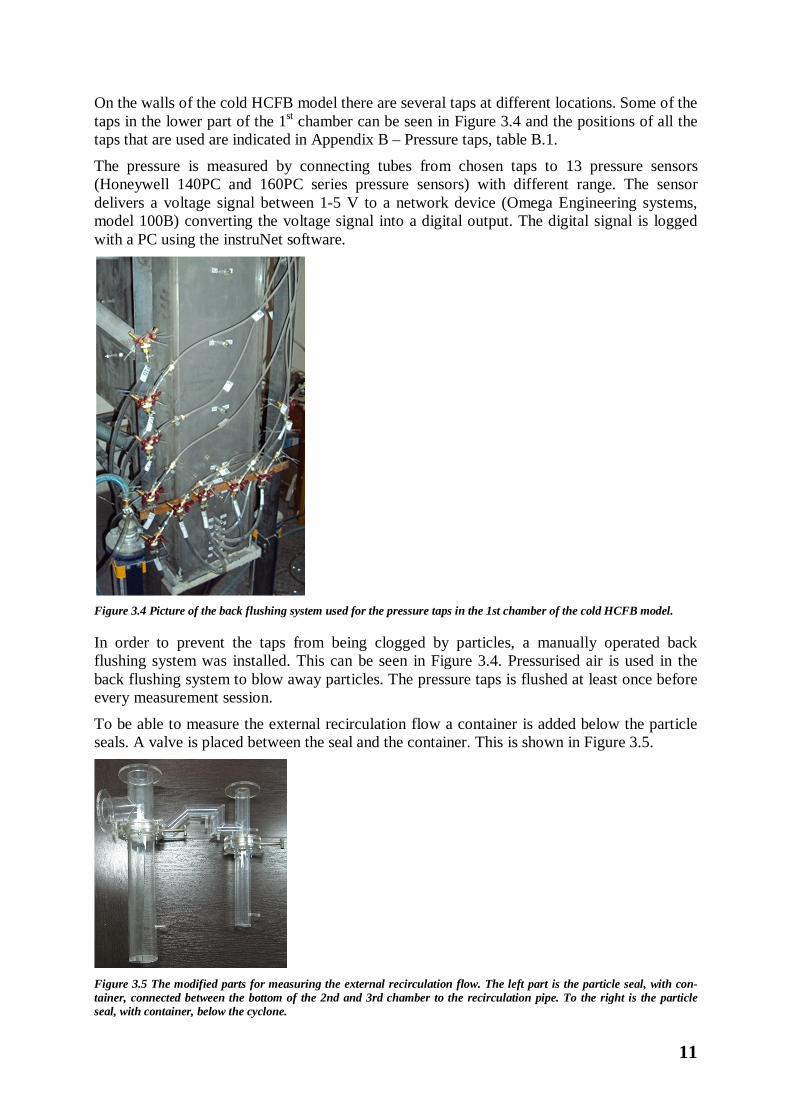
On the walls of the cold HCFB model there are several taps at different locations. Some of the taps in the lower part of the 1st chamber can be seen in Figure 3.4 and the positions of all the taps that are used are indicated in Appendix B – Pressure taps, table B.1.

The pressure is measured by connecting tubes from chosen taps to 13 pressure sensors (Honeywell 140PC and 160PC series pressure sensors) with different range. The sensor delivers a voltage signal between 1-5 V to a network device (Omega Engineering systems, model 100B) converting the voltage signal into a digital output. The digital signal is logged with a PC using the instruNet software.

Figure 3.4 Picture of the back flushing system used for the pressure taps in the 1st chamber of the cold HCFB model.

In order to prevent the taps from being clogged by particles, a manually operated back flushing system was installed. This can be seen in Figure 3.4. Pressurised air is used in the back flushing system to blow away particles. The pressure taps is flushed at least once before every measurement session.

To be able to measure the external recirculation flow a container is added below the particle seals. A valve is placed between the seal and the container. This is shown in Figure 3.5.

Figure 3.5 The modified parts for measuring the external recirculation flow. The left part is the particle seal, with con-tainer, connected between the bottom of the 2nd and 3rd chamber to the recirculation pipe. To the right is the particle seal, with container, below the cyclone.

12

3.2 Industrial HCFB boiler The industrial HCFB boiler examined is located at Kings Paper, Xiamen, China. The boiler has a capacity of 15 metric tonnes of steam per hour, equal to about 12 MWth, and its function is to supply steam to the paper machine. A schematic picture of the boiler is shown in Figure 3.6.

Figure 3.6 Schematic picture of the industrial HCFB boiler located in Xiamen, China. A) Distribution plate. B) Coal feed. C) Rice husk feed. D) Flue gas exit. E) External recirculation from the cyclone. F) External recirculation from the bottom of the 2nd and 3rd chamber. Numbers, 1-5, indicate the locations of the pressure taps.

The five pressure taps used can be seen in Figure 3.6 and their distances from the distribution plate are shown in Appendix B – Pressure taps, table B.2. The taps are back flushed once every day to make sure that they are not clogged. The pressure taps are connected to the sensors (Honeywell 140PC and 160PC series pressure sensors). The signals of the pressure drop were detected and logged in the same way as for the cold model tests.

The external recirculation at the Xiamen boiler is divided into three streams, two from the bottom of the 2nd and 3rd chamber and one from the two cyclones. The two cyclones are connected in parallel and located next to each other, but only one cannot be seen in Figure 3.6. Samples of the bed material are taken from the bottom bed, bottom of the 2nd and 3rd chamber and from the cyclone.

3.3 Running conditions The Xiamen boiler is run with a very low circulation of bed material and therefore the running conditions for the cold HCFB model is calculated by scaling the running condition of the Chalmers boiler instead, representing the classical CFB design. This is done by using

13

Glicksman’s simplified set of parameters presented in Chapter 2, Section 2.3 Glicksman’s scaling laws. The mean pathway in the HCFB model, see Figure 3.7, is assumed to represent the entire height (mean pathway) in the Chalmers boiler. The 1st chamber of the cold HCFB model will therefore represent the first 4.3 m of the Chalmers boiler. Scaling down fluidisation velocity and the bed mass within this first part of the Chalmers boiler gives a fluidisation velocity of 1.70 m/s and a bed mass of 10.0 kg for the 1st chamber of the cold HCFB model. These conditions are the case around which the parameters are varied in order to obtain the other cases. The model is run at ambient condition and air is used as fluidising medium.

In Table 3.1 the scaled values for the Xiamen boiler are given. The scaling factor is 7.8, which is based on the ratio of the hydraulic diameters of the two reactors respectively. As can be seen the row for the height of the 1st chamber in the table, the height ratio in the cold HCFB model is not equal to the scaling factor.

Table 3.1 Actual and ideally scaled quantities for the Xiamen boiler compared to quantities in the cold HCFB model.

Quantity Xiamen HCFB boiler

According to scaling laws

Cold HCFB model

Unit

Bed material Coal ash & rice husk -- Iron particles

1st chamber hydraulic diameter L (2.34) L / 7.8 (0.3) L / 7.8 (0.3) (m)

1st chamber height H (8.2) H / 7.8 (1.1) H / 5.5 (1.5) (m)

Geometry H/L (3.5) H/L (3.5) H/L (5) (-)

Temperature 715 20 20 °C

Gas density 0.35 1.18 1.18 kg/m3

Solid density ρs (2450) 3.4 ρs (8240) 3.2ρs (7900) (kg/m3)

Fluidising velocity u0 (4.8) 0.36 u0 (1.72) 0.35 u0 (1.70) (m/s)

Particle diameter bottom bed dp1 (950) 0.21 dp1 (204) 0.06 dp1 (58**) (µm)

Particle diameter BSTC* dp2 (96) 0.22 dp2 (21) 0.60 dp2 (58**) (µm)

Particle diameter cyclone dp3 (69) 0.22 dp3 (15) 0.84 dp3 (58**) (µm)

Gas dynamic viscosity 43*10-6 18.2*10-6 18.2*10-6 Pa s * BSTC: Bottom of 2nd and 3rd chamber ** Mean particle size of material used in cold HCFB model

The scaled quantities in Table 3.1 are obtained using the simplified Glicksman parameters, see Chapter 2 Theory. Since no combustion takes place in the cold model it is run at ambient temperature and therefore the rest of the parameters needs to adapt to this difference. Bed material used in the Xiamen boiler is coal ash and rice husk, yielding a scaled theoretical solid density of 8 240 kg/m3. Iron particles, which are used in the cold HCFB model, have a solid density of 7 900 kg/m3. The fluidising velocity is changed during the tests in the cold HCFB model, but the main velocity used is the 1.7 m/s. This is also the velocity obtained when scaling the Chalmers boiler. The particle size distribution (PSD) of the bed material in the Xiamen boiler before it is used, cannot be obtained and therefore the fractions in bottom bed

14

of 1st chambers, bottom of 2nd and 3rd chamber and cyclone is presented separately. These are compared to the mean particle size of the iron particles used in the cold HCFB model. The geometry cannot be put in one single value, since all lengths should be uniform, which they are not. In Appendix A – Drawings, all measures are shown for the cold HCFB model, Figure A1, and the Xiamen boiler, Figure A.2. Still, a number has been calculated in order to represent the geometry in the table; height divided by the hydraulic diameter. The solid density should be 3.5 times larger in the cold HCFB model than the Xiamen boiler. It is 3.2 times larger. The density of the gas and dynamic viscosity of the gas follows from the temperature and pressure and hence cannot be influenced by choice.

In Table 3.2 the actual quantities for the Chalmers boiler and its ideally scaled values are presented together with the quantities of the cold HCFB model. The Chalmers boiler has a heat capacity of 12 MWth. Since the main difference between the HCFB and the CFB is the design, the geometry is not fulfilling the scaling criteria. The true height of 13 m in the Chalmers boiler is set to correspond to the mean path way in the cold HCFB model, see Figure 3.7. The scaling factor between the cold HCFB model and the Chalmers boiler is 5 and is calculated as the ratio between the hydraulic diameters of the two reactors respectively. Since the height of the Chalmers is set to represent the mean pathway in the cold HCFB model as well, there a two scaling factors present in Table 3.2. However, the height scaling is used when scaling the bed mass in order to obtain the right conditions, while the hydraulic diameter is used when scaling the simplified set of parameters according to Glicksman.

Table 3.2 Actual and ideally scaled quantities for the Chalmers boiler compared to the quantities for the cold HCFB model.

Quantity Chalmers CFB boiler

According to scaling laws

Cold HCFB model

Unit

Bed material Silica sand & wood chips -- Iron particles

1st chamber hydraulic diameter

L (1.51) L/5 (0.3) L/5 (0.3) (m)

1st chamber height H (4.3*) H/3.6 (1.2) H/3.6 (1.2) (m)

Geometry H/L (2.8) H/L (2.8) H/L (4) (-)

Temperature 850 20 20 °C

Gas density 0.30 1.18 1.18 kg/m3

Solid density ρs (2600) 3.9 ρs (10100) 3.0 ρs (7900) (kg/m3)

Fluidising velocity u0 (3.8) 0.44 u0 (1.69) 0.45 u0 (1.70) (m/s)

Particle diameter dp (280) 0.24 dp (67) 0.21 dp (58) (µm)

Gas dynamic viscosity 47.1*10-6 18.2*10-6 18.2*10-6 Pa s

* True height of the Chalmers boiler is 13 m.

15

The bed material in the Chalmers boiler is silica sand and wood chips. According to the scaling laws, the solid density of the bed material and the temperature of 850 °C require particle density of 10 100 kg/m3 to be used in the cold HCFB model. This is 2200 kg/m3 heavier than the iron particles used. Gas density and dynamic viscosity are temperature and pressure dependent quantities that cannot be influenced without changing gas medium.

Not included in neither of the tables is the particle size distribution (PSD) of the materials nor is the sphericity, φ. These parameters should be similar for both model and industrial boiler. Due to the small size of the particles, the requirements on the sphericity is relaxed and assumed to be sufficient. The PSD however is rather equal in the Chalmers boiler and the cold HCFB boiler but different between the Xiamen boiler and the cold HCFB model. As a complement to Glicksman scaling laws, Geldart’s powder classification can be used to validate that the particles have similar fluidising properties. The iron particles used in the cold HCFB model is classified as group B particles according to Geldart powder classification. So are the mean particles of the bed material in the Xiamen boiler and also the silica sand particles used in the Chalmers boiler. This implies that the three different bed materials all have similar fluidising properties and are comparable (Geldart, 1972).

3.4 Preparations Before the measurements some preparations has to be done. Most of the preparations are per-formed before every measurement but the calibration of the pressure sensors is performed once.

3.4.1 Calibration of pressure sensors The pressure sensor measures the differential pressure between the two locations it is connected to. The sensors are calibrated in order to be able to convert the voltage signal into a pressure. During the calibration, the sensor is connected to a U-tube filled with water. The system is pressurised. The voltage signal is logged by the computer for 30 seconds and the height difference is measured using a ruler. The sensors are valid for different ranges and the procedure described is performed five times for those with a wide range, greater than 2 kPa, and ten for those with a narrow range, less than 0.3 kPa. In addition to these calibration measurements one more is performed for a differential pressure of zero. The pressure measured by the U-tube is calculated with equation 3.1.

∆푃 = 휌 푔∆퐻 (3.1)

Here is ρw the density of water at room temperature, 푔 is the acceleration due to gravity and ∆퐻 is the height difference between the water levels in the U-tube. The pressures obtained from the U-tube are linked together with the corresponding voltages from the sensors and used to form a relation between the voltage and pressure difference. The relation between the differential pressure, ∆푃, and the voltage, U, is assumed to be linear resulting in a general equation as equation 3.2.

∆푃 = 푘 푈 + 푚 (3.2) The range and deviation of the pressure sensors is presented in Appendix C – Pressure sensors, Table C.1.

3.4.2 Preparations for the cold HCFB model The preparation procedure for the cold HCFB model consists of eight steps. 1) Choosing pressure taps. The taps used is decided by the purpose of the measurement. Two pressure sensors are connected to a Pitot tube in order to measure the fluidisation velocity. 2) Add the

16

amount of bed material needed. 3) Turn on the fan and adjust the air flow. 4) Adjust the support air in order to achieve a proper external recirculation. 5) Wait for steady state. 6) Control if the bed mass and fluidisation velocity is within the accepted deviation, 1 kg and 0.05 m/s respectively. 7) Flush the pressure taps. 8) Start the measurements.

3.5 Measurements Independent of the purpose of a boiler it will have to operate at different loads in order to meet a changing demand in a sufficient way. The load is adjusted by changing the fuel and air supply hence also the fluidisation velocity. It is therefore important to assure that the boiler can have a stable operation in a span of fluidisation velocity corresponding to the excepted load variations. The bed mass is changing continuously due to ash formation during combustion, as described earlier. The CFB boiler has therefore to operate correctly for a wide span of bed mass as well. Fluidisation velocity and bed mass are therefore two important factors regarding operation of fluidised bed boilers. This is the reason for investigating the impact of changes in these parameters.

3.5.1 Preparations for the industrial HCFB boiler The preparation procedure for the industrial HCFB boiler in Xiamen consists of four steps. 1) Flushing the pressure taps. Performed once very day. 2) Adjust the fluidisation velocity by changing the frequency of the supply air fan. 3) Wait for steady state. 4) Start the measure-ments. There is one additional step for adding or removing bed mass in the cases with varying bed mass. This is performed between step 2 and 3. Steady state in step 3) is defined as when the temperature in the industrial HCFB boiler is stable, i.e. fluctuating within a couple of degrees, in the bottom bed and the top of the 1st chamber for a fixed fluidising velocity.

3.5.2 Measurements in the cold HCFB model The pressure measurement last for 5 minutes. During that time the bed height is measured and photos taken. When the pressure measurement is done a sample of the bed material in the bottom of the 1st chamber is taken by opening one of the pressure taps. The external recircu-lation flow of bed material to the 1st chamber is measured when the other measurements are accomplished. First, the recirculation flow from the cyclone is measured. The valve added to the loop seal is opened and the support air is turned off in order to extract bed material. The time for the extraction is measured manually with a stop watch and afterwards the volume of the extracted material is measured. The external recirculation flow from the bottom of the 2nd and 3rd chamber to the 1st chamber is measured in the same way. A sample of the bed material from the cyclone and the bottom of the 2nd and 3rd chamber is taken from the extracted particles after the recirculation measurements. The size of the particles in the different samples is determined by using a laser diffraction system (Malvern, Mastersizer 2000) and the density by using a gas pycnometer (Micromeritics, AccuPyc 1330).

3.5.3 Measurements at the industrial HCFB boiler At the Xiamen boiler the duration of pressure measurements is 30 minutes. For two cases (Run1 and Run2) samples of bed material were taken from the 1st chamber, the bottom of the 2nd and 3rd chamber and the cyclone. In Run2, 0.4 m3 of bed material is added compared to Run1. The sizes of the particles are determined by using a mechanically vibrating sieve and the density by using a gas pycnometer (Micromeritics, AccuPyc 1330).

17

3.6 Use of data Data collected during operation is sometimes used for calculations in order to obtain the desired information. In this section, it is briefly explained how this information is calculated.

Fluidisation velocity The fluidisation velocity of the cold HCFB model is obtained by using a Pitot tube located one meter downstream of one of the turns in the air pipe. Due to the turn, the flow at the measuring position is not fully developed. A six point measurement is performed in order to obtain a profile of the flow. The profile is then used to link velocity in one of the six locations to the fluidisation velocity. This location and its relation to fluidisation velocity are assumed to be rather constant in the fluidisation velocity range of 0.9 – 2.1 m/s. The fluidisation velocity of the industrial boiler in Xiamen is estimated from the frequency of the air supply fan. The relation between flow and fan frequency is assumed to be linear.

Pressure profiles The obtained pressure values are put together in order to create a pressure profile. Since the total pressure drop in the cold HCFB model and the Chalmers boiler is different, some adjustments need to be made in order to compare the profiles of the two reactors. This is done by using the mean path way, see Figure 3.7, and the scaled bed mass of the Chalmers boiler, which is calculated to 10.0 kg in Section 3.3. Running conditions. Since the bed mass in both the cold HCFB model and the Chalmers boiler is calculated from the pressure drop, it is possible to set the pressure drop in the 1st chamber of the cold HCFB model and the pressure drop over the corresponding height in the Chalmers boiler, 4.3 m, to be equal. By doing this, the pressure profile is adjusted according to Glicksman’s second parameter, G2, and the mean path way.

Concentration of particles The data obtained from the pressure measurement in the cold HCFB model and in the Xiamen boiler is used to calculate the particle distribution. The concentration of bed material, ρc [kg/m3], is related to the differential pressure as shown in equation (3.3).

휌 = ∆∆

(3.3)

In equation (3.3) the influence from the air density is neglected, since the suspension density is expected to be at least an order of magnitude higher than the air density. The relation between the particle concentration and differential pressure is not valid within the 2nd chamber since the flow is directed downwards. The measured external recirculation flow from both the cyclone and the 2nd and 3rd chamber to the 1st chamber is used in order estimate the concen-tration in the 2nd chamber. Assuming steady state gives a constant concentration and particle flux in the 2nd chamber, 퐺 , [kg/m2s], equal to the total external particle recirculation flux, 퐺 , [kg/m2s]. Also assuming that the particle velocity, up [m/s], is equal to the fluidisation velocity, u0 [m/s], results in equation (3.4).

휌 , = , (3.4)

To make it easier to follow the variations throughout the reactors, the particle concentrations and pressures are plotted against the mean pathway. The definition of the mean pathway for the cold HCFB model is indicated in Figure 3.7. For the Chalmers boiler, the mean pathway is the same as the height from the bottom to the height of the cyclone entrance.

18

3.7 The dashed line shows the defined mean pathway in the cold HCFB model.

The particle concentration in the cold HCFB model is scaled in the comparison to the Chalmers boiler in order to make the comparison valid. The concentration in the HCFB model would otherwise be higher due to the higher particle density. The concentration of the bed material in the bottom bed is therefore set to be the same in both the Chalmers boiler and the cold HCFB model during the comparison.

External and internal recirculation flux of bed material The volume of the bed material extracted during the tests and the time for the extraction are used to calculate the external recirculation flux of bed material. Using the density of the iron particles, a mass flow is obtained. The mass flow is then divided by the cross-sectional area of the first chambers in order to obtain the flux, according to equation (3.5):

퐺 , =∗

(3.5)

Where Gs,ext [kg/m2s] is the recirculation flux of material, V [m3] is the volume of material extracted, ρbm [kg/m3] is the bulk density of the iron particles, τ [s] is the time for the extraction of the volume V and 퐴 [m2] is the cross-sectional area of the 1st chamber.

The internal recirculation flux of bed material is not measured, but calculated from the concentration of particles above the splash zone in the 1st chamber and the concentration in the 2nd chamber. The internal recirculation flux is approximated as the difference in concen-tration between these measurement points and calculated as:

퐺 , = 푢 (휌 − 휌 ) eq. (3.6)

Where Gs,int [kg/m2s] is the internal recirculation flux of material, 휌 and 휌 [kg/m3] is the concentration of particles in the 2nd chamber and above the splash zone in 1st chamber respectively and u0 is the fluidising velocity, which is used since the particle velocity is estimated to be equal to the fluidising velocity. The concentration of material in the 1st chamber is measured with pressure sensors while the concentration in the 2nd chambers is calculated from the total external recirculation flow from cyclone and bottom of 2nd and 3rd chambers to the 1st chamber.

19

Cyclone load The cyclone load, Lcyc [kg/s], is obtained directly from the measurement of recirculation flow from the cyclone to the 1st chamber.

퐿 = ∗ (3.7)

The cyclone load for the Chalmers boiler is calculated from equation (3.8).

퐿 , = 퐺 , ∗ 퐴 (3.8)

Before using this equation the recirculation flux and cross-sectional area of the Chalmers boiler is scaled according to the Glicksman scaling laws.

21

4 Results In this chapter the pressure measurements and concentration of bed material for the cold HCFB model and Xiamen boiler is presented. Also, both measured and visually observed results from investigation of the bottom bed, particle size distribution, fractionation and recirculation when changing the fluidisation velocities and bed mass separately in the cold HCFB model is presented. Comparison with the Xiamen boiler and Chalmers boiler is made whenever data is sufficient and feasible.

4.1 Bottom bed height The dense region in the bottom of the 1st chamber is referred to as the bottom bed. In a transparent cold HCFB model this phenomenon can be observed visually and measured with a ruler. In Figure 4.1 the results of these measurements can be seen for varying bed mass and fixed fluidisation velocity in A and varying fluidisation velocity and fixed bed mass in B.

Figure 4.1 Bottom bed height on the y-axis at A: Varied bed mass and fixed fluidisation velocity of 1.7 m/s and B: Varied fluidisation velocity and fixed bed mass of 10.0 kg.

For the case with 1.5 kg bed mass and 1.7 m/s, no bottom bed is observed. In all other cases there are a visible bottom bed and its height increases with increased bed mass up to 10 cm using 18.5 kg as bed mass, than it decreases to 7.5 cm in the 23.0 kg of bed mass case.

From Figure 1.1B it is seen that at the first increase in fluidisation velocity the bed height increases from 7 cm to 8 cm. After that it decreases to about 3 cm in the 1.7 m/s case and the 2.0 m/s case.

4.2 Recirculation flux of bed material Since the cold HCFB model is constructed in a transparent plastic material the external and internal recirculation flow of bed material can be observed visually. This is demonstrated in Figure 4.2. The red arrows show the external recirculation flow. One flow comes from the bottom of 2nd and 3rd chamber (large vertical arrow) and the other from the cyclone (small vertical arrow). Before entering the 1st chamber the two recirculation flows joins in one flow.

A B

22

The internal recirculation of bed material becomes visible since the iron particles on the wall appear in a light grey colour in contrast to the dark grey colour otherwise. The internal recirculation flow occurs all over the walls in the 1st chamber.

Figure 4.2 Photo of cold model during operation. External recirculation of bed material is marked with arrows and part of internal recirculation with an ellipse.

The procedure to find the quantity of the recirculation flows are described in Chapter 3, Section 3.6 Use of data. 4.2.1 External recirculation Bed mass and fluidising velocity influence the quantity of the recirculation flux of bed material (G [kg/m2s]) from bottom of 2nd and 3rd chambers and cyclone to 1st chamber. In Figure 4.3A the recirculation flux from cyclone to 1st chamber and from bottom of 2nd and 3rd chamber to 1st chamber as well as the total external recirculation at different bed mass is presented. It is shown that the external recirculation increases with increased bed mass.

Figure 4.3 External recirculation flux of bed material to 1st chamber from bottom of 2nd and 3rd chamber (BSTC) and from cyclone. A: Varied bed mass and fixed fluidising velocity of 1.7m/s. B: Varied fluidisation velocity and fixed bed mass of 10.0 kg.

External Internal

Bottom of 2nd and 3rd

1st Chamber

Cyclone

A B

23

The recirculation flux of bed material from the cyclone to the 1st chamber is in the range of 0.5 kg/m2s to 1 kg/m2s for the cases of 5.5, 10.0 and 23.0 kg of bed mass. In the case with 15.5 kg bed mass the recirculation flux from the cyclone is 4 kg/m2s. Keeping the bed mass fixed and increasing the fluidising velocity, increases the recirculation flux from the bottom of 2nd and 3rd chambers and lowers the recirculation flux from the cyclone, shown in Figure 4.3B.

4.2.2 Internal recirculation Internal recirculation flux is calculated from the concentration in 1st and 2nd chamber. In Figure 4.4A and 4.4B the influence on internal recirculation from changes in bed mass and fluidising velocity are presented respectively.

Figure 4.4 Internal recirculation flux of bed material in 1st chamber. A: Fixed fluidisation velocity of 1.7 m/s and varied bed mass B: Fixed bed mass of 10.0 kg and varied fluidisation velocity.

Increased fluidising velocity increases the internal recirculation flux from 16 kg/m2s in the case of 1.0 m/s to 93 kg/m2s in the case of 1.7 m/s. Varying the bed mass at fixed fluidisation velocity yields an increase from 5.5 kg to 10.0 kg of bed mass. At 15.5 kg of bed mass the internal recirculation flux of bed material is lower than at 10.0 kg of bed mass. At 23.0 kg of bed mass the highest internal recirculation flux, 127 kg/m2s, is obtained.

4.2.3 Comparison between internal and external recirculation Table 4.1 presents the external and internal share of the total recirculation flux of bed material for the five cases shown in Figure 4.4A and 4.4B.

A B

24

Table 4.1 Share of internal and external recirculation flux of bed material for five cases with varied bed mass and varied velocity. BSTC: Bottom of 2nd and 3rd chamber.

Case 5.5 kg 1.7 m/s

10.0 kg 1.7 m/s

15.5 kg 1.7 m/s

23.0 kg 1.7 m/s

10.0 kg 1.0 m/s

Internal recirculation flux 1st chamber 83% 86% 75% 80% 71%

External recirculation flux BSTC - 1st chamber 17% 14% 21% 20% 24%

External recirculation flux Cyclone - 1st chamber 0.6% 0.4% 4.4% 0.6% 4.5%

Total recirculation flux 77 109 93 159 22 kg/m2s

The share of internal recirculation flux of bed material is in the range of 71%-86% of the total recirculation flux. It is lowest for the case of 10.0 kg of bed mass and 1.0 m/s, which also is the case with lowest total recirculation flux. The highest total recirculation flux is measured for the case with highest bed mass. In the Chalmers boiler, Johnsson et al. (1998) have estimated the total recirculation of bed material to be 40 kg/m2s of which 75% is internal and 25% is external. In a CFB boiler all the external recirculation flow comes from the cyclone.

4.3 Pressure measurements In the following section the pressure profiles for the cold HCFB model and the Xiamen boiler are presented. There is also a general comparison between the HCFB boiler type and the ordinary CFB boiler, which is represented by the cold HCFB model and the Chalmers boiler respectively.

4.3.1 Influence of bed mass Figure 4.5 shows the pressure profiles for six different bed masses at a constant fluidisation velocity of 1.7 m/s. The 1.5 kg and 23.0 kg cases have the lowest and highest inlet absolute pressure respectively and the others follow the same pattern in between. Throughout the 1st chamber some lines do on the other hand cross each other.

25

Figure 4.5 Measured pressures along the mean pathway for cases with varied bed mass and fixed fluidisation velocity of 1.7 m/s. Dashed lines indicate the transition to the 2nd and 3rd chamber respectively.

Figure 4.6 presents the pressure drop in the 1st chamber without the effects of the recircu-lation; see section 4.3.3 Effects from external recirculation flow. Here it is shown that the pressure drop increases with an increased bed mass. The second pressure point indicates equal pressure for both the 1.5 kg and 5.5 kg cases and the 15.5 kg and 18.5 kg cases respectively.

Figure 4.6 Pressure drop in 1st chamber at fixed fluidisation velocity of 1.7 m/s and varied bed mass.

4.3.2 Influence of fluidisation velocity Figure 4.7 shows the pressure along the mean pathway at varied fluidisation velocities. There is a difference in inlet pressure which increases with increasing fluidisation velocity.

26

Figure 4.7 Measure pressure along the mean pathway at fixed bed mass of 10.0kg and varied fluidisation velocity. Dashed lines indicate the transition to the 2nd and 3rd chamber respectively.

The individual pressure drop, excluding the recirculation effects, for the four different velocities can be seen in Figure 4.8. Here it is shown that the pressure profiles differ from each other even though the total pressure drop is similar for all the velocities.

Figure 4.8 Pressure drop for fixed bed mass of 10.0 kg and varied fluidisation velocity in the 1st chamber.

4.3.3 Effects from external recirculation flow Figure 4.9 shows a photo of the inlet of the external recirculation pipe to the 1st chamber. Since the cold HCFB model is running at low bed mass it is possible to see how the recircu-lating material falls down towards the distribution plate.

27

Figure 4.9 Photo of the recirculating material entering above the distribution plate in the 1st chamber. The recirculation pipe is marked in red in order to visualize it. The higher concentration to the right is caused by the recirculation.

The recirculation flow that is visualised at the low concentration in the photo is also seen in the results of the pressure measurement. Since these effects disturb the pressure measuring in the lower part of the 1st chamber and thereby the concentration values as well, the effects need to be treated in some way. Therefore they were examined closer, which can be seen in Figure 4.10. From the figure it is seen that the pressure decrease heavily in the beginning which is expected, but then it peaks to a high value and then decreases very fast again, just to increase in the next pressure tap. After this, the pressure stabilises.

Figure 4.10 Measured pressures in 1st chamber with dense spacing between pressure taps at height corresponding to inlet of external recirculation.

During the test of the recirculation effects in the 1st chamber both bed mass and fluidisation velocity was varied in order to see if different conditions influenced the recirculation effect in different ways. In the case with a bed mass of 1.5 kg there is no apparent effects on the pressure profile from the recirculation. Figure 4.11 illustrates the difference between the original profile and the reduced profile, without the points in the region affected by the recirculation, for the 1.5 kg case. Since there is no big difference between the reduced profile and the original profile, the former are assumed to be representative and therefore sufficient to use as a complement to the original measurements.

28

Figure 4.11 Two pressure curves for the case of 1.5 kg of bed mass and 1.7 m/s of fluidising velocity. Blue curve include measuring points in the recirculation region and red curve does not.

Figure 4.12 shows that the reduced curves can be used to show the general tendencies even for the fluidisation velocity comparison.

Figure 4.12 Two pressure curves for the case of 10.0 kg of bed mass and 1.0 m/s of fluidising velocity. Blue curve include measuring points in the recirculation region and red curve does not.

4.3.4 Pressure measurement in the 2nd chamber Figure 4.5 and 4.7 shows that the pressure in the 3rd chamber is much lower than in the 1st chamber. In Figure 4.13 it can be seen that the pressure is relatively constant in the 2nd chamber and that a pressure drop occurs in the entrance to the 3rd chamber. The figure also illustrates that the magnitude of the drop differs between the three cases and that it is the highest velocity that corresponds to the pressure drop of greatest amplitude.

29

Figure 4.13 Measured pressure along the entire mean pathway, including 2nd chamber at varying bed mass and fluidisation velocity. Dashed lines indicate the transition to the 2nd and 3rd chamber respectively.

4.3.5 Industrial HCFB boiler In the same way as for the cold HCFB model the pressure throughout the Xiamen boiler was studied with respect to both bed mass and fluidisation velocity. The results from these measurements will be presented below.

4.3.5.1 Influence of bed mass The influence of changed bed mass in the Xiamen boiler can be seen in Figure 4.14. These results indicates that a higher bed mass corresponds to a greater pressure drop. In the low bed mass case there is a pressure increase in the 2nd chamber which the other cases did not show any tendencies of.

Figure 4.14 Measured pressures along the mean pathway in the Xiamen boiler for varied bed mass. Dashed lines indicate the transition to the 2nd and 3rd chamber respectively.

30

Table 4.2, presents the data of the running conditions corresponding to the results in Figure 4.14. The data indicates that there were some changes in temperature and fluidisation velocity between the three cases.

Table 4.2 Data from runs with varied bed mass at the Xiamen boiler.

Reference

More bed mass

Less bed mass

Temperature 722 687 692 K

Fluidisation velocity 4.93 4.75 4.84 m/s

Fan frequency 2.90 2.91 2.94 Hz

Wind box 5.16 5.18 5.14 kPa

4.3.5.2 Influence of fluidisation velocity The result from three runs with different fluidisation velocities in the Xiamen boiler can be seen in Figure 4.15. In these runs there has been a pressure increase in the 2nd chamber for all three cases.

Figure 4.15 Measured pressure along the mean pathway in the Xiamen boiler for varied fluidising velocity. Dashed lines indicate the transition to the 2nd and 3rd chamber respectively.

In Table 4.3 it can be seen that the fluidisation velocities did not differ that much between the three cases. What is notable is that the temperature changed and thereby affected the velocity in the opposite direction from what was intended.

31

Table 4.3 Data of the running conditions with varied fluidisation velocity in the Xiamen boiler.

Medium velocity

Low velocity

High velocity




Wind box 5.20 4.95 4.78 kPa

4.3.6 Comparison between the HCFB boiler and the classical CFB boiler A comparison between the cold HCFB model and the Chalmers boiler can be seen in Figure 4.16. In order to make a valid comparison between these two, the parameters are adjusted and weighted since both running condition and size differs, see Chapter 3, Section 3.6 Use of data. The dashed lines indicate the borders of the different chambers in the HCFB and have nothing to do with the ordinary CFB boiler else than for the comparison.

Figure 4.16 Pressure curves throughout the Chalmers boiler (CFB) and the cold HCFB model respectively. Dashed lines indicate the transition to the 2nd and 3rd chamber respectively, for the cold HCFB model.

4.3.7 Reference measurements Two kinds of reference measurements were performed. One was without bed material in order to examine how the particles influence the pressure. Another was to verify that there were no differences in the results, if the same conditions were examined several times independent of each other.

4.3.7.1 Without bed material Figure 4.17A shows how the pressure varies throughout the cold HCFB model when it is empty and the recirculation pipe is blocked. In the usual case, the particles seal the recircu-lation pipe and force the air to pass through the three chambers. Therefore the recirculation is blocked manually this time in order to obtain the right conditions.

32

The profile indicates that there is a pressure increase in the bottom of the 1st chamber for all three cases even though the amplitude varies. Even though the 2.8 m/s has both the highest and lowest pressure drop throughout the reactor it ends up having the highest total pressure drop. Hence the figure indicates that the total pressure drop increase with a higher air velocity. The highest pressure per meter is in the entrance to the 3rd chamber in all cases.

Figure 4.17B contains a comparison between when the cold HCFB model is run empty with and without blocked recirculation at an air velocity of 1.7 m/s. Even though the two measurements have different resolution it is possible to see some similarities, e.g. pressure increases in the beginning. It is also possible to see some differences e.g. total pressure drop is slightly bigger in the unblocked case.

Figure 4.17 A) Pressure profile when the cold HCFB model is empty and with blocked recirculation at three different air velocities. B) Difference between blocked and unblocked cold HCFB model when it is empty at air velocity of 1.7m/s. Dashed lines indicate the transition to the 2nd and 3rd chamber respectively.

A B

33

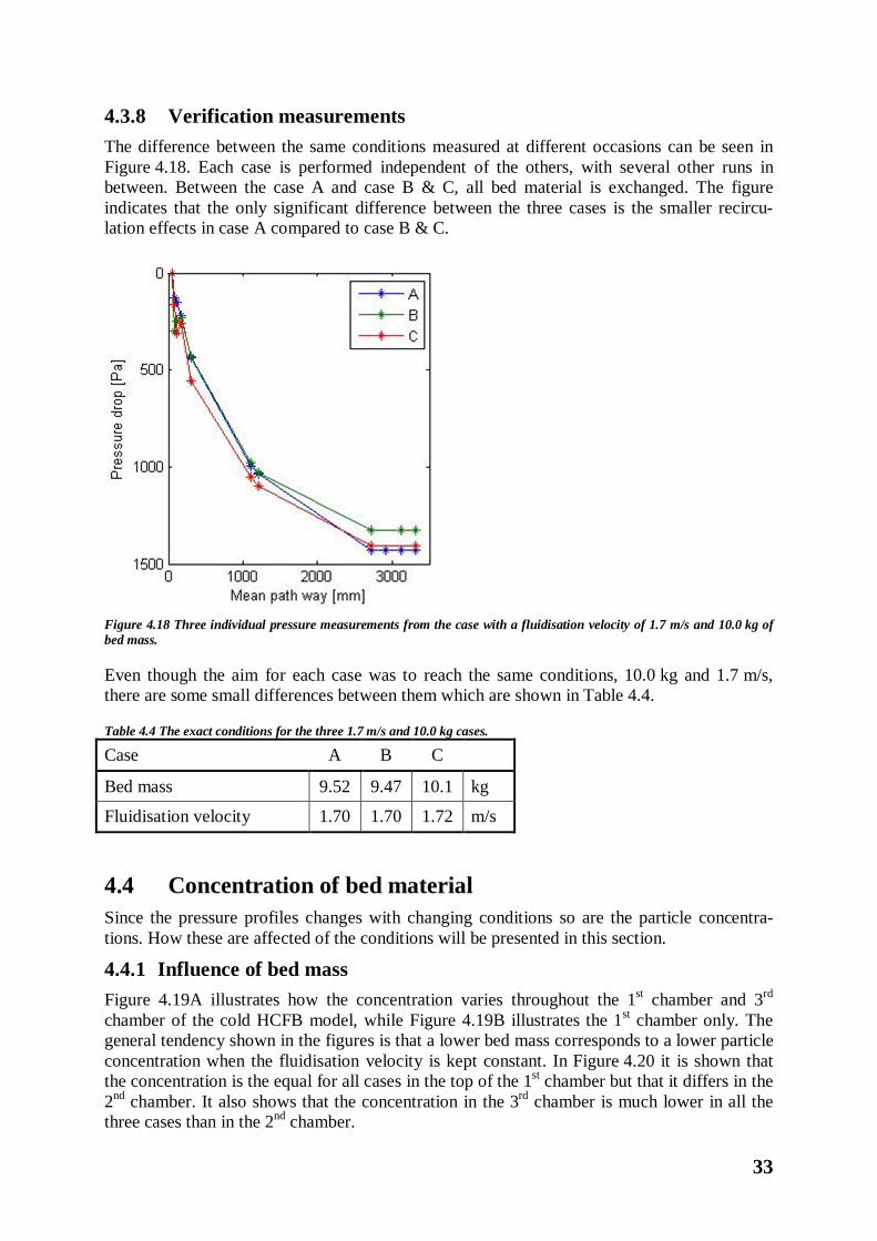
4.3.8 Verification measurements The difference between the same conditions measured at different occasions can be seen in Figure 4.18. Each case is performed independent of the others, with several other runs in between. Between the case A and case B & C, all bed material is exchanged. The figure indicates that the only significant difference between the three cases is the smaller recircu-lation effects in case A compared to case B & C.

Figure 4.18 Three individual pressure measurements from the case with a fluidisation velocity of 1.7 m/s and 10.0 kg of bed mass.

Even though the aim for each case was to reach the same conditions, 10.0 kg and 1.7 m/s, there are some small differences between them which are shown in Table 4.4.

Table 4.4 The exact conditions for the three 1.7 m/s and 10.0 kg cases.

Case A B C

Bed mass 9.52 9.47 10.1 kg


4.4 Concentration of bed material Since the pressure profiles changes with changing conditions so are the particle concentra-tions. How these are affected of the conditions will be presented in this section.

4.4.1 Influence of bed mass Figure 4.19A illustrates how the concentration varies throughout the 1st chamber and 3rd chamber of the cold HCFB model, while Figure 4.19B illustrates the 1st chamber only. The general tendency shown in the figures is that a lower bed mass corresponds to a lower particle concentration when the fluidisation velocity is kept constant. In Figure 4.20 it is shown that the concentration is the equal for all cases in the top of the 1st chamber but that it differs in the 2nd chamber. It also shows that the concentration in the 3rd chamber is much lower in all the three cases than in the 2nd chamber.

34

Figure 4.19 A) Particle concentration throughout the 1st and 3rd chamber for the cold HCFB model at fixed fluidisation velocity of 1.7 m/s and varied bed mass. B) The same case but focus on the 1st chamber. “ * ” indicates values based on pressure measurement “ o ” indicates values calculated or measured not using pressure.

As can be seen in Figure 4.19A the concentration in the 3rd chamber is first and fore most very low compared to the 1st chamber. As mentioned in section 3.5 Use of data the density of air is neglected. As the results shows the concentration, or the suspension density, is in the same order of magnitude as the density of air. If the density of air is taken into consideration some of the particle concentration in the 3rd chamber will be negative which is not possible. Therefore the concentration in the 3rd chamber is too low to be measured with the equipment used hence it is only possible to say that the concentration is low. The concentration in the 3rd chamber is further analysed in the Section 4.4.5 Cyclone load.

Figure 4.20 Particle concentrations throughout the entire cold HCFB model at a fluidisation velocity of 1.7 m/s and varied bed mass. Dashed lines indicate the transition to the 2nd and 3rd chamber respectively. “ * ” indicates values based on pressure measurement “ o ” indicates values calculated or measured not using pressure.

A B

35

4.4.2 Influence of fluidisation velocity Figure 4.21A shows how changes in fluidisation velocity influence the concentration in 1st and 3rd chamber and Figure 4.21B shows the same but only for 1st chamber. It can be seen that the lower the velocities are, the higher the concentrations are in the bottom part of the 1st chamber. Then it shifts and throughout the rest of the pathway the higher velocities have the higher concentrations.

Figure 4.21 Particle concentration along the mean pathway at fixed bed mass and varied fluidisation velocity. A: 1st and 3rd chamber B: 1st chamber. Dashed lines indicate the transition to the 2nd and 3rd chamber respectively. “ * ” indicates values based on pressure measurement “ o ” indicates values calculated or measured not using pressure.

Figure 4.22 indicates that the concentration increases from the top of the 1st chamber into the 2nd chamber for the 1.0 m/s case.

Figure 4.22 Particle concentrations for the entire cold HCFB model at a constant bed mass of 10.0 kg and varied fluidisation velocity. Dashed lines indicate the transition to the 2nd and 3rd chamber respectively. “ * ” indicates values based on pressure measurement “ o ” indicates values calculated or measured not using pressure.

A B

36

4.4.3 Industrial HCFB boiler Tests of the influence from bed mass and fluidisation velocity on the particle concentration is performed in the Xiamen boiler as well.

4.4.3.1 Influence of bed mass Figure 4.23 illustrates the mean particle concentrations in the 1st and 3rd chamber in the Xiamen boiler at three different bed masses. Due to that the first pressure tap is placed 1.30 m above the distribution plate the concentration is only measured above that position in the 1st chamber. The figure shows that the measured concentrations are below 1.8 kg/m3 for all three cases. The relative concentration between the three cases changes so that the location with the highest concentration in the 1st chamber has the lowest concentration in the 3rd chamber and so on. The density of air cannot be neglected in the 3rd chamber for the same reasons as in the cold model. And once again the results can only be used to say that that concentration is low relative the other chambers but no exact numbers.

Figure 4.23 Mean particle concentrations in the 1st and 3rd chamber in the Xiamen boiler at three different bed mass.

Table 4.5 include condition data from the Xiamen boiler at the three different bed masses examined. Here it is shown that there is some variation in the conditions between the three cases.

Table 4.5 Condition data for three different bed mass at the Xiamen boiler.

Reference

More bed mass

Less bed mass




Fuel feeder frequency 20.5 20.2 18.2 Hz

37

4.4.3.2 Influence of fluidisation velocity Figure 4.24 shows the measured concentration in the 1st and 3rd chamber of the Xiamen boiler at three different fluidisation velocities. In this experiment the concentration in the 1st chamber reaches levels above 2 kg/m3. The relative concentration between the three cases changes so that the location with the highest concentration in the 1st chamber has the lowest concentration in the 3rd chamber and so on.

Figure 4.24 Mean concentrations in the 1st and 3rd chamber of the Xiamen boiler at varied fluidisation velocity.

Table 4.6 contains condition data from the Xiamen boiler at the three different velocities. It shows that the fuel feed is rather constant during the low and high velocity but in the medium case the fuel feed frequency is almost half.

Table 4.6 Condition data for three different velocities at the Xiamen boiler

Medium Low

velocity High

velocity




Fuel feeder frequency 7.55 13.8 13.7 Hz

4.4.4 Comparison between the HCFB boiler and the classical CFB boiler Figure 4.25 shows the concentration for both the Chalmers boiler and also the cold HCFB model. Due to their difference in size and running condition the parameters are scaled and weighted to obtain a valid comparison between these two. In Chapter 3, Section 3.6 Use of data it is explained how this is done. The dashed lines indicate the borders of the different chambers in the HCFB and have nothing to do with the ordinary CFB boiler else than for the comparison. The figures indicate that the bottom bed is higher in the Chalmers boiler than in the cold HCFB model and that the concentration is higher in the Chalmers boiler along the first 15%

38

of the pathway. After 15% they change relatively to each other and it is the cold HCFB model that has the higher concentration until the flow enters the 2nd chamber where the lines, once again, crosses each other. After the flow in the cold HCFB model has entered the 2nd chamber, the concentration in the cold HCFB model keeps below the concentration in the Chalmers boiler along the rest of the pathway.

Figure 4.25 Concentration throughout the Chalmers boiler’s mean pathway (CFB) and the cold HCFB model’s mean pathway. Dashed lines indicate the transition to the 2nd and 3rd chamber respectively, for the cold HCFB model.

4.4.5 Cyclone load In Chapter 4, Section 4.2 Recirculation flux of bed material it is shown that the flow through the cyclone was low in both relative and absolute numbers. Since the efficiency of the cyclone is high, the flow out from the cyclone is used to estimate a cyclone load. This is presented in Table 4.7.

Table 4.7 The measured cyclone load at varied fluidisation velocity and varied bed mass respectively Bed mass Fluidisation Velocity

5.5 kg 10.0 kg 15.5 kg 18.5 kg 23.0 kg

1.0 m/s 0.09 kg/s 1.2 m/s 0.13 kg/s 1.7 m/s 0.04 0.14 0.37 0.06 0.08 kg/s

In the Chalmers boiler, the cyclone load is 22.9 kg/s according to Johnsson et al (1998). If this value is scaled down to the conditions in the cold HCFB model, it corresponds to a load of 6.2 kg/s. That is about one order of magnitude higher than the loads of the cold HCFB model.

4.5 Particle size distribution and fractionation In this section the particle size distribution (PSD) and the mean particle size at different locations, i.e. the fractionation, in the cold HCFB model, the industrial HCFB boiler and the industrial CFB boiler will be presented. Particle sizes in figures are not scaled. In Table 4.10, however, the scaled values are presented in order to make a comparison between the reactors.

39

4.5.1 Cold HCFB model The PSD of the bed material in the cold HCFB model is very narrow. This is expected since the iron particles used are manufactured for a certain particle size. There are some differences in sizes which can be seen in Figure 4.26 and due to this it is possible to obtain a fractionation in the cold HCFB model.

Figure 4.26 Mass fraction versus particle size in the cold HCFB model for the standard case of 10.0 kg and 1.7 m/s. The blue line represent bed material from bottom bed, the red line represent bed material from bottom of 2nd and 3rd chamber and the green line represent bed material from cyclone.

4.5.1.1 Influence of bed mass Investigations show that different bed mass and fluidisation velocity have an impact on the fractionation. Figure 4.27 shows the fractionation between bottom bed, bottom of 2nd and 3rd chamber and cyclone for two different bed mass at the equal velocity in the cold HCFB model.

Figure 4.27 Fractionation in the cold HCFB model. Mean particle size of bed material on the cold HCFB model extracted from bottom bed, bottom of 2nd and 3rd chamber (BSTC) and cyclone respectively. Two different tests at varied bed mass and fixed fluidisation velocity of 1.7 m/s.

Mas

s fra

ctio

n (%

)

Particle size (µm)

Cum

ulat

ive

mas

s fra

ctio

n (%

)

40

The difference in mean particle size is larger between bottom of 2nd and 3rd chamber and the cyclone than between the bottom bed and bottom of 2nd and 3rd chamber. There is also a small difference in mean particle size at all locations between the two cases. The mean particle sizes together with D(0.1) and D(0.9) are presented in Table 4.8. D(0.1) is the size at which 10% of the particles are smaller than or equal to. D(0.9) is the size at which 90% of the particles are smaller than or equal to and D(0.5) is the mean particle size.

Table 4.8 Fractionation in the cold HCFB model. Particle sizes, D(0.1), D(0.5) and D(0.9) of bed material extracted from bottom bed, bottom of 2nd and 3rd chamber and cyclone respectively in the cold HCFB model. Varied bed mass and fixed fluidisation velocity of 1.7 m/s.

Bed mass 5.5 kg 23.0 kg

D(0.1) D(0.5) D(0.9) D(0.1) D(0.5) D(0.9)

Bottom bed 40.6 61.9 93.8 35.6 58.0 91.8 µm

BSTC 37.3 59.2 92.1 36.9 58.6 91.4 µm

Cyclone 19.8 35.5 61.6 18.6 32.3 55.2 µm BSTC: Bottom of 2nd and 3rd chamber. D(0.1) is the size at which 10% of the particles are smaller than or equal to. D(0.9) is the size at which 90% of the particles are smaller than or equal to and D(0.5) is the mean particle size.

As can be seen from the table, the smallest 10% of the particles in the 5.5 kg-case are slightly larger than the smallest 10% in the 23.0 kg-case at all locations respectively. Comparing the span between D(0.1) and D(0.9) at all locations shows that the span is larger in the bottom bed for the 23.0 kg case (56.2 µm) than for the 5.5 kg case (53.2 µm). In the bottom of 2nd and 3rd chamber, the span is almost the same but in the cyclone the span is now larger in the 5.5 kg case than in the 23.0 kg-case, 41.8 µm and 36.6 µm respectively.

4.5.1.2 Influence of fluidisation velocity Another parameter influencing the fractionation is the fluidisation velocity. Results from experiments at fixed bed mass and different velocities are presented in Figure 4.28 and the mean particle sizes from the figure are found in Table 4.9.

Figure 4.28 Fractionation in the cold HCFB model. Mean particle size of bed material in cold HCFB model extracted from bottom bed, bottom of 2nd and 3rd chamber (BSTC) and cyclone. Fixed bed mass of 10.0 kg and varied fluidisation velocity.

41

There is a distinct fractionation between bottom of 2nd and 3rd chamber and cyclone but not so distinct between the bottom bed and bottom of 2nd and 3rd chamber. An increase in velocity results in a lower mean particle size in the bottom bed and a higher mean particle size in the cyclone. In the bottom of 2nd and 3rd chamber the change is smaller than for the cyclone and bottom bed. However in Table 4.9 the values show that there is a small increase in the mean particle size in the bottom of 2nd and 3rd chamber between velocity 1.2 and 1.7 m/s, but almost no change between 1.7 m/s and 2.0 m/s.

Table 4.9 Fractionation in the cold HCFB model. Particle sizes, D(0.1), D(0.5) and D(0.9) of bed material extracted from bottom bed, bottom of 2nd and 3rd chamber and cyclone respectively in the cold HCFB model. Varied fluidisation velocity and fixed bed mass of 10.0 kg.

Fluidising velocity 1.2 m/s 1.7 m/s 2.0 m/s

D(0.1) D(0.5) D(0.9) D(0.1) D(0.5) D(0.9) D(0.1) D(0.5) D(0.9) Bottom bed 45.4 64.2 90.4 43.4 63.2 91.5 41.7 62.1 91.9 µm

BSTC 40.3 60.2 89.0 43.4 60.8 85.2 41.3 60.9 89.0 µm

Cyclone 27.1 45.3 73.5 30.4 48.7 76.5 29.9 49.9 80.5 µm BSTC: Bottom of 2nd and 3rd chamber. D(0.1) is the size at which 10% of the particles are smaller than or equal to. D(0.9) is the size at which 90% of the particles are smaller than or equal to and D(0.5) is the mean particle size.

Looking at the smallest value of D(0.9), it is found in the cyclone at 1.2 m/s, while the largest value of D(0.9) is found in the bottom bed at 2.0 m/s.

4.5.2 Industrial HCFB boiler Char combustion and abrasion are two causes that make the size of particles in an industrial boiler to change during operation. These phenomenons cause a continuous change in the span of the particle size distribution (PSD). So does the adding of new fuel and removing of fly ash. Therefore the PSD in an industrial boiler covers a wide range of particle sizes compared to the PSD in a cold HCFB model, which does not have these phenomenon or factors that influence the PSD.

42

In Figure 4.29 the PSD for the Xiamen boiler at two different running conditions are presented. The amount of bed material is higher in Run2 than Run1.

Figure 4.29 Mass fraction versus particle size of bed material extracted from the bottom bed, bottom of 2nd and 3rd chamber (BSTC) and cyclone in the Xiamen boiler. Bed mass is lower in Run1 than Run2.

A difference in PSD of the bed material is seen in the bottom of 2nd and 3rd chamber for the two running conditions, Run1 and Run2. In the bottom bed and the cyclone the difference in PSD is not obvious even though it can be seen that the cyclone has a small increase in particle size in Run2 while the bottom bed has a little decrease in mean particle size in Run2. Since the sieving equipment only allowed particles up to 6 mm to be determined the largest particles in the bottom bed in the Xiamen boiler were not size determined. However, their weight is included in the test, hence the cumulative mass fraction for the bottom bed ends below unity. Particles larger than 6 mm are shown in Figure 4.30.

Figure 4.30 Photo of the largest (>6000µm) particles in the bottom bed of the Xiamen boiler.

In the Xiamen boiler it is the leftovers from coal combustion that is used as bed material. As Figure 4.30 shows, the largest particles are stones that have been enclosed within the coal supplied to the boiler.

43

Looking at the samples extracted from the bottom of the 2nd and 3rd chamber in the Xiamen boiler it is possible to see that it contain some char from the rice husk. Even though they are very fragile there is still a lot left after taking them out of the boiler indicating that it is actually even more within the boiler. Figure 4.31 shows two samples extracted from the bottom of the 2nd and 3rd chamber. Figure 4.31A shows the 900-1250 µm which despites its volume contributes to less than 0.1% of the mass fraction. Figure 4.31B shows a sample of particles in the size range of 61-90 µm also from the bottom of the 2nd and 3rd chamber. This is the fraction having the highest mass fraction, 21%. The volume fraction on the other hand do not differ so much between the 900-1250 µm and 61-90 µm indicating a significant variation in density of the particles.

Figure 4.31 Pictures of two samples taken from the bottom of the 2nd and 3rd chamber at the Xiamen boiler. A: Fraction containing rice husk ash, size: 900-1250 µm. B Fraction with highest mass, size: 60-90 µm.

4.5.2.1 Influence of bed mass Experiments with different bed mass in the Xiamen boiler shows a lower mean particle size in the bottom bed at higher bed mass and larger mean particle size in the cyclone at higher bed mass, see Figure 4.32.

Figure 4.32 Fractionation in the Xiamen boiler. Mean particle size of bed material extracted from bottom bed, bottom of 2nd and 3rd chamber (BSTC) and cyclone. Run1 has a lower bed mass than Run2.

A B

44

The mean particle diameter in the bottom of 2nd and 3trd chamber is 96 µm in Run1 and decreases to 90 µm in Run2. In the cyclone, the mean particle diameter increases from 69 µm to 72 µm for the two different cases.

4.5.3 Comparison between the HCFB boiler and the classical CFB boiler From comparing the PSD in the Xiamen boiler with the PSD in the Chalmers boiler, Figure 4.33 is yielded. Note that the Chalmers boiler and the Xiamen boiler are two different kinds of CFB boilers. Therefore there is one less curve for the Chalmers boiler.

Figure 4.33 Mass fraction versus particle size of bed material extracted from the bottom bed, bottom of 2nd and 3rd chamber (BSTC) and cyclone during Run2 in the Xiamen boiler compared to bed material extracted from the bottom bed and cyclone in the Chalmers boiler (Åmand et al., 1999).

It can be seen from Figure 4.33 that the Chalmers boiler has a narrower PSD than the Xiamen boiler. Particles in the bottom bed of the Xiamen boiler are larger than in the bottom bed of the Chalmers boiler while in the cyclone the particles are smaller in the Xiamen boiler than in the Chalmers boiler. Table 4.10 shows the particle sizes D(0.1), D(0.5) and D(0.9) of the bed material in the bottom bed, bottom of 2nd and 3rd chambers and cyclone for the cold HCFB model and the Xiamen boiler. The corresponding sizes for the Chalmers boiler in the bottom bed and cyclone are also included. The particles sizes in the industrial boilers are scaled using G3 to be comparable to the particles sizes in the cold HCFB model. G3 does not include the particle size directly but since the minimum fluidisation velocity, umf, is dependent on the particle size, G3 can be used for scaling the particles. Difference between D(0.9) and D(0.1) is presented as span.

45

Table 4.10 Particle size of bed material for the cold HCFB model compared to scaled particle size of bed material for the Xiamen boiler and the Chalmers boiler.

D(0.1) D(0.5) D(0.9) Span

Cold HCFB model

Bottom bed 43 63 91 48 µm

BSTC 43 61 85 42 µm

Cyclone 30 49 77 46 µm

Xiamen HCFB

Bottom bed 96 204 665 568 µm

BSTC 11 21 65 54 µm

Cyclone 10 15 28 18 µm

Chalmers CFB

Bottom bed 50* 70* 105* 56 µm

Cyclone 39* 61* 70* 31 µm * Values for the Chalmers boiler are obtained from Åmand et al. (1999) D(0.1): size at which 10% of the particles are smaller than or equal to. D(0.9): size at which 90% of the particles are smaller than or equal to. D(0.5): mean particle size. Span: difference between D(0.9) and D(0.1). BSTC: Bottom of 2nd and 3rd chamber

Mean particle size of bed material in the bottom bed of the Xiamen boiler is more than 3 times larger than the mean particle size in the bottom bed of the cold HCFB model. In the bottom of 2nd and 3rd chamber and the cyclone the mean particle size is about 3 times larger in the cold HCFB model than the Xiamen boiler. The span between D(0.9) and D(0.1) is between 42 µm and 48 µm in the cold HCFB model while it is between 18 µm and 568 µm in the Xiamen boiler. The D(0.9) in the cyclone of the Xiamen boiler is smaller than the D(0.1) in the cyclone of the cold HCFB model. Compared to the cold HCFB model, the Chalmers boiler has a larger mean particle size of the bed material in both the bottom bed and the cyclone. The particles in the cyclone of the Chalmers boiler have the same mean particle size as particles in the bottom of 2nd and 3rd chamber in the cold HCFB model. To highlight the difference in fractionation between the cold HCFB model, the Xiamen boiler and the Chalmers boiler a normalized mean particle size for each reactor is presented in Figure 4.34. The particle sizes are normalized to the mean particle size in the bottom bed of each reactor respectively.

46

Figure 4.34 Normalized mean particle size in the cold lab rig, the Xiamen boiler and the Chalmers boiler. The values are normalized to the mean particle size in the bottom bed for each reactor respectively.

In the Xiamen boiler, the mean particle size in the bottom of 2nd and 3rd chamber is 10 % of the mean particle diameter in the bottom bed and in the cyclone it is further reduced to about 7 %. Corresponding values for the cold lab rig is 96 % and 77 % respectively.

4.6 Visual observations One of the great advantages with a transparent cold HCFB model is the possibility to observe the flow visually. Figure 4.35 shows three photos, A, B and C. Photo A and B illustrates high and low concentration respectively in the 2nd chamber. It can be seen that the particles tend to be in the right part of the 2nd chamber for cases A and B. Hence the concentration over the cross sectional area is unevenly distributed. In the area between the main flow of the 2nd chamber and the wall between the 1st and the 2nd chamber, the flow creates a swirl rotating clockwise. Due to this the particles in that area take part in some kind of internal recirculation in an upwards direction. These particles are taken from the top layer of the buffer build up in the left side of the bottom of 2nd and 3rd chamber.

47

Figure 4.35 Visual observation of particle concentration in cold HCFB model. A: High particle concentration. B: Low particle concentration. C: Same concentration as in A, but bottom of 2nd and 3rd chamber zoomed in.

In the 3rd chamber it is possible to observe an internal recirculation on three of four walls. The fourth wall is the one to the right in Figure 4.35A and is heavily affected by the flow of air from the 2nd chamber. This flow forces the material on the right side of the bottom of 2nd and 3rd chamber to lift and move up the right wall. This prevents the internal recirculating particle on this wall from returning to the bottom of 2nd and 3rd chamber. In Figure 4.35B it is possible to see that not all of the particles making it to the top of the 1st chamber, fall over into the 2nd chamber. Instead they fall down again, taking part in the internal recirculation. This is the case also with a higher concentration as in A, even though it is hard to see in the photo. Figure 4.35A and –B indicates that the amount of particles stored in the bottom of 2nd and 3rd chamber varies with the fluidisation velocity and particle concentration. The amount of particles was built up until the angle of the pile was too steep and it collapsed. This caused some of the particles to fall down into the recirculation pipe in the bottom of the bottom of 2nd and 3rd chamber. The collapses were small and frequent which created an almost continuous flow into the recirculation pipe. The time between two “collapses” was never longer than a couple of seconds hence it were no problem to make an average over a longer time for the pressure measurements. Figure 4.35C shows a close up of the bottom of 2nd and 3rd chamber for the same case as in Figure 4.35A. Here it is easier to see that there is an even higher amount of particles in the bottom of 2nd and 3rd chamber on both sides compared to Figure 4.35B. In the same way as on the left hand side of the bottom of 2nd and 3rd chamber are the top layer particles on the right hand side also carried away. Here they enter the 3rd chamber and due to the air flow, most of the particles in the bottom of the 3rd chamber are close to the right wall. This makes the cross sectional concentration unevenly distributed also in the 3rd chamber. In the 3rd chamber it seems to be more evenly distributed further up, at least the difference over the cross section is too small to be visible observed.

A B C

49

5 Discussion The discussion is dived into three parts. Initially the results of changing the two parameters; bed mass and fluidisation velocity in the cold HCFB model, will be discussed. Thereafter follows two sections of comparing the results of the cold HCFB model with an industrial HCFB boiler and with a classical CFB boiler respectively.

5.1 Cold HCFB model Using a transparent cold HCFB model gives many advantages when it comes to visualisation and opportunities of controlling the operation. However, the setup has also had its limitations which have affected the work and some of the results. To clarify which results that might be influenced and in what way, the possible obstacles are discussed in connection to the results it affects.

5.1.1 Scaling The cold HCFB model used is not perfectly down-scaled from a specific boiler. Instead, it is a general representation of a HCFB boiler. For this thesis however, it is important to know how close the model is to the industrial boilers it is compared to. To determine this, Glickman’s scaling laws have been used.

The first parameter, G1, regards the fluidisation velocity which in the Xiamen boiler is 4.8 m/s and in the Chalmers boiler 3.8 m/s. When scaling these values, they become about 1.7 m/s in both cases. This is why the cold HCFB model has been running at that velocity when changing bed mass. The second parameter, G2, is the density scaling, which is very close in the case of the Xiamen HCFB boiler and sufficient when it comes to the Chalmers boiler. The third and the seventh parameter, G3 and G7, are related to the minimum fluidisation velocity and particle size distribution (PSD) respectively. The minimum fluidisation velocity is dependent on the particle size which is why this parameter is used to scale the size of the particles. To fulfil the criteria for the Xiamen boiler, the plan was to use iron particles of three different mean particles sizes where each size corresponded to the size in one of the chambers. Unfortunately, it was discovered after the experiments that two of the three sizes of the iron particles delivered were not of the sizes that they were labelled. Instead all particles were of the same size. Still, it has been possible to measure the fractionation between the chambers in the cold HCFB model and also compare it to the industrial HCFB and CFB boilers. The size of the iron particles used is a bit larger than the mean size of the particles in the bottom of 2nd and 3rd chamber of the Xiamen boiler and thus it is fairly well representing the particles that are leaving the bottom bed. Fourth parameter, G4, scales the recirculation flux of bed material. This was not possible to measure in Xiamen, but has been measured in the cold HCFB model. If all other scaling parameters would have been fulfilled, the recirculation flux in the Xiamen boiler could have been estimated from the recirculation in the cold HCFB. Geometry is the fifth parameter, G5, of the simplified Glicksman parameters. As can be seen by comparing the drawings of the cold HCFB model and the industrial HCFB boiler, the geometry of the two reactors differs. This parameter is hard to express in a number but a try is made in Table 3.1. In the table, the height in relation to the hydraulic diameter of the boiler is used to represent the geometry. What cannot be told from this value is that the top of the model is flat, while the top of the Xiamen boiler is angled. This makes the height in the Xiamen boiler different depending on where one measures. Also, the cross-sectional area is quadratic in the 1st and 2nd chamber in the model but not in the Xiamen boiler. In addition to

50

this, the change in cross-sectional area between the chambers is different in the model compared to the Xiamen boiler, which can be seen in Appendix A – Drawings. What also differs is the number of cyclones and the size and design of the recirculation paths. All geometry parameters influence the possibilities of exactly representing the Xiamen boiler with the cold HCFB model. However, having this in mind, some general and accurate conclusions about the behaviour of a HCFB boiler can be made with the HCFB model. The similarities in geometry between the Chalmers CFB boiler and the cold HCFB model are not so many. Still the scaling is used to get some kind of comparison. Finally, the sphericity of the particles used should also be equal, G6. But this criterion can also be relaxed since all the others are far from exact.

5.1.2 Bottom bed Proving the existence of a bottom bed is simple in a transparent cold HCFB model since it is visible for the eye and can be photographed. At constant bed mass and increasing fluidisation velocity, the height of the bottom bed decreases. The reason for this is found in the concen-tration profile of the particles. It shows a higher particle concentration in the transport zone at higher velocities. An increased concentration within a zone yields an increased pressure drop in the corresponding zone. Since the bed mass is defined as the weight of the particles in the 1st chamber, it is directly related to the pressure drop. An increased pressure drop in the transport zone implies that the pressure drop in the bottom bed should be decreased since the bed mass is kept constant. From this, it is obvious that the height of the bottom bed should decrease with increasing velocity. This is seen in Figure 4.1B, with an exception for the 1.2 m/s case. The reason for this exception can be found in the problem of measuring an exact height of the bottom bed. An increased bed mass on the other hand, yields a higher bottom bed. This is rather straight-forward since the amount of particles in the 1st chamber should by definition be increased if the bed mass is increased at constant velocity. The added material will then be divided between the three zones in the 1st chamber; bottom bed, splash zone and transport zone. The dividing is not equal but to reach steady state the amount of particles in each zone will increase and hence the bed height increases as well.

5.1.3 Recirculation The basis for obtaining the data of the recirculation measurements is the extraction of bed material during operation. Since extraction of bed material lowers the bed mass and thereby affects the running condition, this measurement could only be performed once for each test. As it turned out, it was quite difficult to do the measurement and therefore some of the cases lack information regarding this part. The major problem was measuring the recirculation from the bottom of 2nd and 3rd chamber due to the high flow rate. Another problem rose due to that the particles leaving the bottom of 2nd and 3rd chamber were supposed to fall right into the particle extractor and not be forced into the 1st chamber. Therefore the support air needed to be turned off. When turning off the support air the material in the recirculation was no longer fluidised and therefore did not flow as easily as it did during normal operation. This some-times resulted in plugging that stopped the flow for a short time and then released much material in very short time. For the cases in which the measurement could not be performed accurately enough, the results are not presented. The aim of this measurement was not to find the exact recirculation flux but to get an indication about the order of magnitude of the recirculation flux.

51

As is seen in Figure 4.3A and –B the external recirculation flux of bed material increases with an increased bed mass and with an increased fluidisation velocity independently. This is expected, since both these changes cause a higher amount of particles leaving the 1st chamber and thereby the recirculation has to increase in order to achieve a steady state. The increased external recirculation flux to the 1st chamber can be seen both from the bottom of 2nd and 3rd chamber and from the cyclone. In the case of 15.5 kg of bed mass the recirculation flux from the cyclone is extra high. In this case, the measurement is a little inaccurate due to the formation of a plug when the support air was turned off. Since the plug could not be seen until the measurement of the recirculation started, it affected the result. Since the other three measurements show a similar trend, the recirculation flux from the cyclone in the 15.5 kg case is disregarded when drawing conclusions.

For the internal recirculation flux of bed material, there is a deviation in the trend caused by the 15.5 kg of bed mass case. This deviation is due to an unexpected decrease in concentration above the splash zone in the 1st chamber for this case, which is the concentration used for calculating the internal recirculation. Since this decrease does not follow the trend for the other concentration of particle curves, it is seen as an error. This error also affects the value of the internal recirculation flux. Disregarding the 15.5 kg case, it is seen that an increase in bed mass and fluidising velocity, independently increases the internal recirculation flux. Even if the amount of internal recirculation flux is increased with these parameters, the share of internal recirculation flux is between 75% and 85%, not following any trend. This seems reasonable since the increased quantity of internal recirculation is caused by an increased concentration in the 1st chamber which also yields an increased external recirculation flux as described above.

As described in Chapter 3 Experimental setup and procedure, the recirculation of bed material paths are equipped with support air nozzles in order to fluidise and help the particles flowing through the recirculation. This support air was measured during all conditions in order to be aware of its contribution to the total air supply. Since the support air at maximum was 0.43% of the primary air flow and usually around 0.2%, its impact on the total volume of the air flow is neglected. However, even a small but intense air flow can impact a pressure measurement, but even that is not probable. This is since they are located far from any pressure tap and are never used more than needed, i.e. not more than that the particle seals was fluidised in order to keep the particle moving through the recirculation pipes.

5.1.4 Pressure measurements and concentration of bed material The total pressure drop over the 1st chamber is of course increasing with respect to increasing bed mass since the bed mass is defined as the weight of the particles in the 1st chamber, which is calculated from the pressure drop in the 1st chamber. Worth noticing is on the other hand that the pressure profiles are indicating the same tendencies for all the bed masses examined. The slopes of the curves, see Figure 4.6, are always steeper in the lower part of the 1st chamber than in the top and the slopes are in general steeper if the bed mass is higher. The pressure drop from the top of the 1st chamber to the bottom of the 3rd chamber does not increase at higher bed mass in the same way as in the 1st chamber. In the 3rd chamber the deviations in absolute pressures between different bed mass are much smaller than in the top of the 1st chamber. Since it is the 15.5 kg case that has the highest absolute pressure in the top of the 1st chamber, it has the highest pressure drop between these two locations. That the absolute pressures in the 3rd chamber are more similar between the cases is not that strange since the outlet from the cyclone is to atmosphere. Therefore the pressure drop over the entrance to the last chamber of the cold HCFB model is more dependent on the absolute pressure in the 2nd chamber than on changes in bed mass.

52

Looking at Figure 4.19B, the trend of the bars shows that a higher bed mass yields a higher concentration of particles. The case of 18.5 kg bed mass or the case of 23.0 kg of bed mass disrupts this trend. A simple and likely explanation for this could be that the measured bed height is wrong. In the same figure it seems as four of the six cases has almost the same concentration of particles in the top of the 1st chamber, but that seems to be unlikely. As Figure 4.35 shows it was possible to observe some changes in concentration visually. For the two cases with the highest bed masses it was hard to observe any significant difference but for the others it was possible to distinguish the different concentrations between the cases. Figure 4.20 indicates that the concentration of particles in the 2nd chamber is different in different cases. By visual observation it is possible to see that an increased concentration in the 1st chamber yields an increased concentration in the 2nd chamber and vice versa. This indicates that the concentration in the top of the 1st chamber differ even though the graph in Figure 4.20 does not show that. The change in flow direction between the 1st and 2nd chamber may influences the pressure measurements, thus yielding a misleading result. The fact that the case with a bed mass of 1.5 kg has an increased concentration of particles in the end of the 1st chamber also supports the theory that there are some geometry effects and that some cases might be more sensitive to this than others. Conclusions regarding this phenomenon would require further investigations. The concentration of particles in the 2nd chamber is constant since the suspension flow in the 2nd chamber is directed downwards and hence all particles entering the top will leave in the bottom. Due to the downward directed flow in the 2nd chamber it was not possible to use the pressure to measure the concentration. Therefore, the external recirculation flows are used in order to calculate a concentration for the 2nd chamber and these calculated values are dis-played in the figures. The concentration of particles was therefore affected by the uncertain-ties in the measurements of the external recirculation flows. As mentioned before the concen-tration in the 2nd chamber should be slightly lower than the concentration in the top of the 1st chamber, since some of the particles in the top will fall down and contribute to the internal recirculation in the 1st chamber. Due to the air supply system used, it was not possible to change the velocity without also changing the pressure of the ingoing air. This can be seen in e.g. Figure 4.7 where the pressure into the cold HCFB model is increased at higher velocities. This increase in pressure is relatively small considering the absolute pressure. Therefore the pressure profiles in the 1st chamber are assumed to only be influenced by the varied fluidisation velocity for the cases with fixed bed mass. If the fluidisation velocity is varied instead of the bed mass there is a clear difference in the concentration profile of particles for the different cases. From the distribution plate up to 300 mm of the 1st chamber the concentration is higher for low fluidisation velocities. Throughout the rest of the chamber the trend changes and it is the higher velocities that have the higher concentration of particles. Lower fluidisation velocities cause a reduction in the lifting force acting on the particles. This leads to a larger amount of the particles in the lower part of the 1st chamber for a low velocity compared to a higher velocity. Since the bed mass is kept constant in the cases when the fluidisation velocity were varied, more particles in the bottom yields less particles in the upper part of the 1st chamber. This can be seen in Figure 4.21 where the concentration is higher in the bottom of the 1st chamber for the lower velocities and that it is the other way around in the top. Regarding the concentration in the 3rd chamber the data is not good enough to make any comparison between the exact values from the cases. This is due to two things; first the pressure drop in the 3rd chamber is in the same range as the error of the pressure transmitters,

53

secondly the density of air cannot be neglected for such low concentrations of particles. If the density is subtracted, many of the concentrations in the 3rd chamber would have become negative which is not possible. This also proves that the pressure sensors used are not sufficient. What can be concluded anyway is that the concentration is always very low. The highest concentration among all cases, both varied bed mass and varied fluidisation velocity, was only 3 kg/m3. This was measured in the first half of the chamber for the case with a bed mass of 10.0 kg and a fluidisation velocity of 1.7 m/s. If the air density of 1.2 kg/m3 is taken into consideration, the particle concentration would be 1.8 kg/m3. Since this low concentration was measured in the bottom, it is even lower in the entrance to the cyclone. So even though it is not possible to tell how it varies with neither bed mass nor fluidisation velocity or tell the exact concentration, it is possible to say that the concentration entering the cyclone always is very low compared to the rest of the cold HCFB model. This is supported by the recirculation measurements presented in Chapter 4, Section 4.2 Recirculation flux of bed material.

As could be seen in Figure 4.35, showing pictures of the cold HCFB model during operation, there are two zones in the bottom of the 2nd and 3rd chamber respectively where particles tend to pile up. The one below the 2nd chamber are more or less completely stagnant. There it is only the particles in the top layer that is moving. This motion is caused by the swirl resulting in an internal recirculation flow upwards in the 2nd chamber. Bellow the 3rd chamber there is a little bit more motion. Here the angle of the particle pile increases until it is too steep and some of the particles fall down into the recirculation pipe. These stagnant zones, especially the one below the 3rd chamber, varied with the running conditions. The fluidisation velocity has the highest impact making the zones bigger with higher velocity. That this affects the zone below the 3rd chamber more is due to the increased force in the higher flow making it possible to have a steeper angle before it falls down. The amount of particles in the stagnant zones changes with changes in bed mass and fluidisation velocity. Hence, an increased fluidisation velocity demands an increase in the total amount of particles in order to keep the bed mass constant. Also, the measured change in bed mass when changing the bed mass is smaller than the actual change due to the stagnant zones.

5.1.5 Particle size distribution and fractionation Even though the PSD for the iron particles in the cold HCFB model is narrow, a distinct fractionation of particles between the bottom of 2nd and 3rd chamber and the cyclone occurs. A well-functioning fractionation in an industrial boiler implies that particles such as unburned char, will not leave the boiler until they have shrank to sizes that are smaller than what the cyclone can separate. This leads to less unburned fuel leaving the boiler with the flue gases and hence a higher combustion efficiency. Comparing the fractionation between varied bed mass, it shows that an increased bed mass yields a smaller mean particle size of the particles in the bottom bed as well as in the cyclone. At the same time the mean particle size in the bottom of 2nd and 3rd chamber is more or less unchanged. Also, looking at the smallest 10%, D(0.1), of the particles in the 5.5 kg-case they are slightly larger than the smallest 10% in the 23.0 kg-case at all locations respectively. This was expected since a larger bed mass has a higher amount of small particles and they will end up in the cyclone. A share of 10% of the particles in the cyclone for the higher bed mass will therefore have a smaller particle size than the corresponding share for the 5.5 kg-case. The same holds for smallest 90%, D(0.9), of the particles in the two cases. However, to draw a conclusion from the increased bed mass, the span between D(0.1) and D(0.9) should be examined.

54

Starting in the bottom bed, the span between D(0.1) and D(0.9) is 53.2 µm at the 5.5 kg-case and 56.2 µm in the 23.0 kg-case, hence a larger span is observed in the case of higher bed mass. This is explained by the fact that at the higher bed mass a larger amount of particles is collected in the bottom bed which implies that less small particles have left the 1st chamber compared to the case with low bed mass. In the bottom of 2nd and 3rd chamber the span is rather equal. But in the cyclone the span is smaller in the case of higher bed mass, 36.6 µm compared to 41.8 µm at the lower bed mass. The reason to the smaller span in the case with higher bed mass is that with an increased amount of particles in the cold HCFB model, the absolute number of small particles has increased. Since the amount of particles in the cyclone is more or less the same between the two cases, the case with the highest amount of small particles in absolute number should have the lowest size span in the cyclone, which it has.

When comparing the impact from varied fluidisation velocity, it seems as increased velocity leads to a smaller mean particle size in the bottom bed. This is reasonable since at higher velocity, larger particles can be elevated over to the 2nd chamber. Also, the recirculation increases at higher velocities and hence the exchange of particles between all locations is higher, yielding a more even mean particle size at all locations. In the cyclone, the higher velocity yields particles with larger mean size. This is due to the same reason as for the particles being smaller in the 1st chamber; larger particles in circulation and higher recircu-lation of smaller particles. To summarize, increased velocity decreases the degree of fraction-ation. Comparing the span between D(0.1) and D(0.9) for all fluidising velocities it is expected that the highest difference would be reached in the case of 2.0 m/s due to the high circulation of material. This is also what the tests show for the bottom bed and the cyclone. In the bottom of 2nd and 3rd chamber however, the span is more or less the same for the lowest and highest velocity, while the 1.7 m/s-case breaks the pattern and shows a much lower span than the other velocities. No logic reason for this decrease in span is found, other than it is an irregularity.

5.1.6 Effects from external recirculation flow It is something happening in the region where the recirculation of particles enters the 1st chamber, which easily can be seen in the figures containing pressure profiles for the first chamber. In the cases presented in Figure 4.10, more pressure sensors have been used for the measurement in the region where the recirculation enters the 1st chamber. In this figure it is clearly shown that the magnitude of the effects varies with the running conditions. The two cases with the highest external recirculation flow also have the largest influence on the pressure measurement from the recirculation. The five pressure taps that seems to be in the affected region are at heights between 87 – 207 mm which can be compared with the recircu-lation pipe that has its centre at 206 mm with a diameter of 80 mm. Some of the taps affected are located below the recirculation pipe, which is not so strange since the particles fell down a bit when they entered the 1st chamber. The fact that the pressure taps affected are located in a region near the recirculation pipe and that the effects change with the change of the magnitude of the recirculation, suggests that it is the recirculation that has caused the unexpected pressure profile for some cases.

5.2 Industrial HCFB boiler It is hard to see any clear pattern in the results obtained from the Xiamen boiler representing the industrial HCFB boiler. There was unfortunately always more than one parameter that changed. During the varied bed mass runs the velocity were supposed to be constant but as the results show, it in fact varied more than it did when the velocity were supposed to be varied.

55

Even though the cold HCFB model is not an exact scale down of the Xiamen boiler, it still represents the general design figures of a HCFB. Therefore the Xiamen boiler should respond in a similar way as the cold HCFB model does when bed mass and fluidisation velocity is varied.

5.2.1 Pressure measurements and concentration of bed material Due to that the pressure in the 1st chamber was measured from a point 1.30 m above the distribution plate to the top, it is not possible to tell anything about what happens below that, which is where the dense region is. This would have been of interest especially since the really low pressure drop, i.e. low concentration of particles, indicates that it is not so much material circulating. Even though the particle density in the Xiamen boiler was low it does not compensate for the extremely low particle concentration. In Figure 4.14 and Figure 4.23 the results for varied bed mass in the Xiamen boiler are shown. It can be seen that it responds in a similar way as the cold HCFB model does even though it might run as a BFB boiler, i.e. increased pressure drop in the 1st chamber with increased bed mass.

Looking at the results from the varied fluidisation velocity it seems as the Xiamen boiler responds in another way than excepted. If a higher velocity causes a higher concentration of particles than the effects of a lower velocity on the concentration, then the medium fluidisation velocity should be in between in order to indicate any pattern. However, this is not the case. The reason could be that the fuel feed is much lower at the medium velocity case compared to the other two cases. Since the feed is located at 2.10 m above the distribution plate, it is included in the pressure measurement in the 1st chamber. Therefore a decrease in fuel feed will cause a lower particle concentration, as in the medium velocity case. If only the low and high fluidisation velocities are considered, where the fuel feed was relative constant in between, it is possible to see that the Xiamen boiler responds in the same way as the cold HCFB model. In order to confirm the influence of both the fuel flow and fluidisation velocity further investigations are needed.

5.2.2 Particle size distribution and fractionation The wide PSD in the Xiamen boiler can partly be explained by the occurrence of abrasion of the bed material but mainly by the use of coal ash as bed material. The coal sometimes used as fuel in the Xiamen boiler contains impurities such as enclosed stones, creating a bed material with fractions of very large particles. To avoid too large particles the bed material is regenerated manually. Also, the main fuel supplied to the boiler is rice husk which in contra-diction to coal has extremely low char content and hence do not contribute to any creation of large particles. These factors are the reason for the wide PSD in the Xiamen boiler. As Figure 4.31 showed it was possible to see that the particles in the bottom of the 2nd and 3rd chamber contained ash shells from the rice husk. Due to their very small particle size it would be reasonable to find some in the cyclone as well. The results did on the other hand not indicate this. Since the ash shells are very fragile they most probably did brake in the cyclone to a larger extent than in the bottom of the 2nd and 3rd chamber. Therefore they formed much smaller particles and were harder to distinguish among the other particles. Interesting to compare between the cold HCFB model and the industrial boiler is the fraction-ation, which is related to the PSD. From Figure 4.34, it can be seen that there is a large difference between the size of the particles in the bottom bed and the bottom of 2nd and 3rd chamber for the Xiamen boiler. This difference is not as large in the cold HCFB model. The main reason for the very large fractionation in between the bottom bed and the bottom of 2nd and 3rd chamber is the large particles shown in Figure 4.30 and the wide PSD range for the Xiamen boiler, Figure 4.33. This together with the low concentration of particles in the

56

transport zones of the Xiamen boiler explains the large difference in mean particle size between the bottom bed and the bottom of 2nd and 3rd chamber. A small circulation of bed material also indicates a small recirculation and thereby the mixing of bed material is less, which creates good condition for higher degree of fractionation. From Figure 4.34 it looks like the fractionation of bed material between the BSTC (bottom of 2nd and 3rd chamber) and the cyclone is lower in the Xiamen boiler than in the cold HCFB model. However, if comparing the ratio of the fractionation between the bottom of 2nd and 3rd chamber and the cyclone for both reactors, it is shown that the fractionation still is higher in the Xiamen boiler. To summarize, due to a larger PSD in the Xiamen boiler it has a higher degree of fractionation. The reason for the difference in the fractionation behaviour of the bed material between the cold HCFB model and the Xiamen boiler could be explained by the low bed mass in the Xiamen boiler. As can be seen in the cold HCFB model, the fractionation between bottom bed and bottom of 2nd and 3rd chamber is higher at low bed mass and the fractionation is lower between bottom of 2nd and 3rd chamber and cyclone at low bed mass. This could indicate that if the cold HCFB model would have been run at an even lower bed mass, the fractionation trend for the two reactors would have been more similar. This is also pointed out in Figure 4.32, fractionation in the Xiamen boiler, where higher bed mass yields lower difference in fractionation between the bottom bed and bottom of 2nd and 3rd chamber.

Since PSD samples were only analysed for two tests when alternating the bed mass, it is not possible to draw a general conclusion. Therefore it can be of interest to further investigate the fractionation with regard to operating conditions and compare the result with both HCFB boilers and CFB boiler, in order to draw conclusions regarding the impact from the design.

5.3 Comparison between the HCFB boiler and the classical CFB boiler

When comparing the pressure profile of the Chalmers CFB boiler to the pressure profile of cold HCFB model, it is possible to see that there are some differences. The pressure drop in the 1st chamber of the HCFB model is almost equal to the pressure drop over the corre-sponding pathway in the CFB, which is expected since it was scaled to be equal. The small deviation that still exists can be explained by that the exactly right conditions were not achieved for the cold HCFB model. Another difference between the pressure profiles occurs during the first part of the pathway, this could be a result of the cold HCFB model not having the same geometry relations as that the Chalmers boiler.

5.3.1 Recirculation The internal recirculation flux of bed material in the Chalmers boiler is expected to be higher than the internal recirculation flux of bed material in the cold HCFB model. This is because the concentration of particles decreases with height in a riser. Hence a CFB boiler should have a smaller share of the total bed material leaving the riser than what is leaving the 1st chamber in a corresponding HCFB boiler. It should be pointed out, that even though the total share of internal recirculating bed material should be lower in a HCFB, the external recirculation from the cyclone to the 1st chamber is expected to be smaller. This is because of the high recircu-lation of particles from the bottom of the 2nd and 3rd chamber to the 1st chamber.

57

However, the share of internal recirculation flux of bed material is rather equal in both the cold HCFB model and the Chalmers boiler. The share of recirculating bed material from the cyclone follows the idea above and is in other words smaller in the cold HCFB model than in the Chalmers boiler. A smaller recirculation flux of bed material from the cyclone implies a lower cyclone load, which is beneficial and further discussed in section 5.3.4 Cyclone load.

5.3.2 Pressure measurements and concentration of bed material The pressure drop in the entrance to the 3rd chamber of the cold HCFB model makes the pressure profiles differ a lot in the last part of the pathway between the cold HCFB model and the CFB boiler. This difference can be explained by the fact that the 3rd chamber only has half of the cross-sectional area compared to the other two chambers. The Chalmers boiler on the other hand has the same cross sectional area along the entire pathway. Maybe the pressure profile would have been more similar if the cross sectional area was kept constant in the cold HCFB model as well. It was possible to obtain the desired bed mass and fluidisation velocity in the cold HCFB model similar to the Chalmers boiler, but not at the same time to obtain a bottom bed height also similar to the Chalmers boiler. Therefore the concentration profiles in Figure 4.25 differ relatively much through the first 10-15% of the pathway. This is also the reason for the difference in pressure profile in Figure 4.16 for the same part. From 15% to 45% of the path-way the lines follow each other as expected. Then after 45% of the pathway there is a large decrease in concentration of particles in the cold HCFB model when the particles enter the 2nd chamber. Due to this decrease in concentration, the pressure drop curve for the cold HCFB model crosses the Chalmers boiler’s line. For the next part, 45%-73% of the pathway, the concentration is naturally constant in the cold HCFB model while it decreases steadily in the Chalmers boiler. When the particles enter the 3rd chamber at 73% of the pathway, concen-tration is almost the same as in the Chalmers boiler. From this point, the concentration decreases in both reactors. The decrease is, however, steeper in the cold HCFB model than the Chalmers boiler. Even though the absolute numbers of the concentration in the 3rd chamber are incorrect there is a large drop in concentration between the 2nd and 3rd chamber as the figures indicates. This is due to the external recirculation of bed material from the bottom of 2nd and 3rd chamber.

That the concentration of particles is lower at the inlet to the cyclone in the HCFB compared to the CFB could be an advantage since the cyclone then could be made smaller which also makes it cheaper to build. Of course, the cyclone is not the only factor that is important. In order for a boiler to deliver the heat that it is supposed to, the heat transfer to the tube walls also needs to be sufficient. The visual observations made in the cold HCFB model have shown that the cross sectional particle concentration is uneven, especially in the 2nd chamber but also in the 3rd chamber. This results means that the heat transfer area is not used in an optimal way.

If the heat transfer surfaces are not used efficiently it will increase the total amount of heat transfer surfaces needed, hence also the cost. In a classical CFB boiler it would have been easy to say that an uneven distributed flow was a disadvantage. Of course it would have been optimal to have an even distribution of bed material in the 2nd chamber of a HCFB boiler as well, but with the current design it is not possible. On the other hand, the wall between the 1st and 2nd chamber uses its both sides for heat transfer. This gives a “bonus side” that is already paid for. This makes a general cost comparison between the two types of boiler a little more complex. The cyclone can be smaller for the HCFB boiler due to the external recirculation from the bottom of the 2nd and 3rd chamber. The heat transfer surfaces on the other hand are

58

not used in the most efficient way, but some of this is compensated by the free “bonus side”. To find out how much and if the total cost will be lower for a HCFB boiler requires a more profound comparison than the research performed in this thesis.

One thing that has to be considered when designing a CFB boiler is problems with erosion from the bed material on the boiler tubes. Erosion can cause severe problems and high expenditures if the boiler tubes brake down due to this. That the flow is forced to change direction within the HCFB will increase the contact between the particles and the tube walls as can be seen clearly in Figure 4.35. It might be possible to make some design changes making the turns smother hence also lower the erosion. For example, the angle of the bottom plates in the bottom of 2nd and 3rd chamber can be changed in order to both reduce the stagnant zones and lower the risk of erosion on the outer wall of the 3rd chamber.

5.3.3 Particle size distribution and fractionation The PSD of the bed material in the Chalmers boiler and the cold HCFB model is relatively similar. This is good from a scaling perspective since one of the parameters requires that the PSD should be similar. The difference in degree of fractionation of bed material is observed between the two reactors. This is also good, since it is expected. The reason to this is the use of two recirculation paths for bed material in the HCFB compared to only one path in the CFB. This makes a less amount of particles going to the cyclone in a HCFB than in a CFB, resulting in a lower cyclone load discussed below.

5.3.4 Cyclone load Since the measuring of the recirculation flow from the cyclone to the 1st chambers is just aiming at giving a point of direction about the flow, the cyclone load should just be seen as a rough estimation. The idea is to confirm the theory that a cyclone in a HCFB can be made smaller than in a CFB, due to the large separation of particles in the bottom of the 2nd and 3rd chamber.

The value for the Chalmers boiler is scaled so that it is possible to compare to the values from the cold HCFB model. Since the scaling criteria are not fulfilled between the Chalmers boiler and the cold HCFB model, the values are not completely comparable. However, it is sufficient to give an indication. In this comparison the cyclone load is about one order of magnitude lower in the cold HCFB model than in the industrial CFB boiler, which confirms the theory that a cyclone in a HCFB can be made smaller than a cyclone for a CFB. A smaller cyclone means lower investment costs.

59

6 Conclusions In this thesis work a lab scale cold model has been used to study the distribution of bed material in a horizontal circulating fluidised bed, HCFB, boiler. Concluding remarks can be given by this study both on the general figures of a HCFB boiler and on its comparison with the classical circulating fluidised bed, CFB, boiler.

Steady-state is possible to achieve for all variations in both fluidisation velocity and bed mass examined in the cold HCFB model.

The distribution of bed material is uneven over the cross section in the 2nd chamber, independent of running conditions in the cold HCFB model.

The cyclone load is much lower in a HCFB boiler than it is in a classical CFB boiler which suggests that the cyclone can be made smaller in a HCFB boiler compared to a CFB boiler. However, some bed material is still found in the cyclone of the cold HCFB model even at low fluidisation velocities, therefore, the cyclone cannot be removed completely.

The degree of fractionation is greater in a HCFB boiler than in a CFB boiler.

61

References Basu, P., Kefa, C., Jestin, L., (2000), Boiler and Burners, Design and theory, New York:

Springer-Verlag, (Mechanical engineering series 28), pp.302-345. Geldart, D., (1972): Types of Gas Fluidization. Powder Technology, Vol. 7, 1973, pp. 285-

295. Glicksman, L.R., (1984): Scaling Relationships for Fluidized Beds, “Chemical Engineering

Science”, Vol. 39, 1984, pp. 1373-1379 Glicksman, L.R., Hyre, M.R., Farrel, P.A., (1994): Dynamic Similarity in Fluidization.

Multiphase flow, Vol. 20, 1994, pp. 331-386. Grace, J.R., Avidan, A.A., Knowlton, T.M., (1997), Circulating Fluidized Beds, Suffolk: St

Edmundsbury Press, pp. 1-20, 417-440. IEA – International Energy Agency http://www.iea.org/stats/coaldata.asp?COUNTRY_CODE=CN [Access date: 2011-05-28] Johansson, A., Johnsson, F., Leckner, B. (2006): Solids back-mixing in CFB boilers.

Chemical Engineering Science, Vol. 62, 2007, pp. 561-573. Johnsson, F., Breitholtz, C., Leckner, B., (1997), “Solids Segregation in a CFB-Boiler

Furnace”, In Proceedings of Fluidization IX, (Eds. Fan, L-S., Knowlton, T.) Engineering Foundation, New York, 1998, pp. 757-764.

Johnsson, F., Sternéus, J., Leckner, B., (2001), Characteristics of gas mixing in a circulating fluidised bed, Powder Technology, Vol. 126, 2002, pp. 28-41

Kullendorff, A. Leckner, B. (1991): Circulating Fluidised Bed Boilers, Report A 91-194, Chalmers University of Technology, Department of Energy Conversion, Gothenburg, Sweden, (1991), pp. 37

Leckner, B., Szentannai, P., Winter, F., (2009) “Scale-up of Fluidized-bed combustion”, In proceedings of Scale-up in combustion, (Ed. Lackner, M.), ProcessEng Engineering GmbH, Vienna, (2009), pp. 1-25.

Leckner, B., Werther, J., (2000), Scale-up of Circulating Fluidized Bed Combustion, Energy and fuels, Vol. 14, 2000, pp. 1286-1292.

Li, L., Tan, Z., Wang, J., Xu, J., Cai, C., Hou, Y., (2011): Energy conservation and emission reduction policies for electric power industry in China. Energy Policy, Vol. 39, 2011, pp. 3669-1679.

Li, Q. H., Zhang Y. G., Meng A. H. ”Design and Application of Novel Horizontal Circulating Fluidized Bed Boiler”, In Proceedings of the 20th International Conference on Fluidized Bed Combustion, (Eds. G. Yue, H. Zhang, C. Zhao, Z. Luo), Tsinghua University Press, Beijing, pp. 206-211, 2009.

UNEP – United Nations Environment Programme (2001): Report of the STAP Selective Review of “China Efficient Industrial Boiler Project, 2001, 18 pp.

Wen, C.Y., Yu, Y.H., (1966): A generalized method for predicting the minimum fluidization velocity. AIChE, Vol. 12, No. 3, 1966, pp. 610-612.

Wolfram Alpha http://www.wolframalpha.com/input/?i=drag+force [Access date: 2011-05-28]

62

Åmand, L.E, Lyngfelt, A., Karlsson, M., Leckner, B., (1999), Fuel loading of a Fluidized Bed Combustor Burning Bituminous Coal, Peat or Wood Chips, Report A 97-221, Chalmers University of Technology, Department of Energy Conversion, Gothenburg, Sweden, (1999), pp. 21

Appendix

A1

Appendix A – Drawings Drawing of the cold HCFB model.

Figure A.1 Drawing of the cold HCFB model

A2

Drawing of the industrial HCFB boiler at King’s Paper, Xiamen, China

Figure A.2 Drawing of the Xiamen HCFB boiler

B1

Appendix B – Pressure taps Position of each pressure tap in the cold HCFB model. Distance along the mean pathway between distribution plate and the pressure tap is also presented.

Table B.1 Position of pressure taps in cold HCFB model

Tap number Chamber

Distance from distribution plate

[mm]

1 1st 46

2 1st 57

3 1st 87

4 1st 117

5 1st 147

6 1st 176

7 1st 207

8 1st 307

9 1st 1106

10 1st 1206

11 2nd 1607

12 2nd 2207

13 3rd 2717

14 3rd 2917

15 3rd 3117

16 3rd 3317

Position of pressure taps in the industrial HCFB boiler in Xiamen, China.

Table B.2 The distance along the mean pathway from distribution plate to the pressure taps used at the Xiamen boiler

Pressure tap 1 2 3 4 5

Distance from distribution plate - 0.40 1.30 4.75 9.35 10.40 m

C1

Appendix C – Pressure sensors From the calibration the ranges of each pressure sensor could be identified. In Table C.1 the average deviation and maximum deviation between the calibration tests are presented for each sensor.

Table C.1 Pressure range, average deviation and maximum deviation for each pressure sensor

Sensor # Number of points, excluding zero

Average deviation

Maximum deviation

Range [Pa]

001 5 0.40% 0.52% 2391

002 5 1.40% 2.17% 2429

005 5 0.18% 0.32% 6051

007 10 1.78% 3.89% 220

010 5 0.29% 0.55% 22661

011 5 0.15% 0.27% 22720

013 10 1.54% 4.51% 214

014 10 2.20% 5.83% 215

016 10 1.36% 2.82% 234

017 10 1.60% 3.91% 212

019 5 0.23% 0.46% 6190

020 5 0.10% 0.15% 6046

022 5 0.36% 0.88% 6138

023 5 0.19% 0.38% 6150

distribution of bed material in a horizontal circulating fluidised bed boiler

Documents