Distributed Structures for Multi-Hop Networks

Rajmohan Rajaraman

Northeastern University

Partly based on a tutorial, joint with Torsten Suel, at the DIMACS Summer School on Foundations of Wireless Networks and Applications, August 2000

September 10, 2002

• routing tables• spanning subgraphs

• spanning trees, broadcast trees

• clusters, dominating sets

• hierarchical network decomposition

Focus of this Tutorial

“We are interested in computing and maintaining

various sorts of global/local structures in

dynamic distributed/multi-hop/wireless networks”

What is Missing?

• Specific ad hoc network routing protocols– Ad Hoc Networking [Perkins 01]– Tutorial by Nitin Vaidya

http://www.crhc.uiuc.edu/~nhv/presentations.html

• Physical and MAC layer issues– Capacity of wireless networks [Gupta-Kumar

00, Grossglauser-Tse 01]

• Fault-tolerance and wireless security

• Introduction (network model, problems, performance measures)

• Part I:

- basics and examples - routing & routing tables

- topology control

• Part II: - spanning trees

- dominating sets & clustering

- hierarchical clustering

Overview

Multi-Hop Network Model

• dynamic network• undirected• sort-of-almost planar?

What is a Hop?

• Broadcast within a certain range– Variable range depending on power control capabilities

• Interference among contending transmissions– MAC layer contention resolution protocols, e.g., IEEE

802.11, Bluetooth

• Packet radio network model (PRN)– Model each hop as a “broadcast hop” and consider

interference in analysis

• Multihop network model– Assume an underlying MAC layer protocol– The network is a dynamic interconnection network

• In practice, both views important

• Wireless Networking work - often heuristic in nature

- few provable bounds

- experimental evaluations in (realistic) settings

• Distributed Computing work - provable bounds

- often worst-case assumptions and general graphs

- often complicated algorithms

- assumptions not always applicable to wireless

Literature

Performance Measures

• Time

• Communication

• Memory requirements• Adaptability• Energy consumption• Other QoS measures

path length

number of messages

correlation

{

}

• Static

• Limited mobility - a few nodes may fail, recover, or be moved (sensor networks)

- tough example: “throw a million nodes out of an airplane”

• Highly adaptive/mobile - tough example: “a hundred airplanes/vehicles moving at high speed”

- impossible (?): “a million mosquitoes with wireless links”

• “Nomadic/viral” model: - disconnected network of highly mobile users

- example: “virus transmission in a population of bluetooth users”

Degrees of Mobility/Adaptability

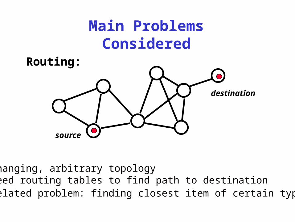
Main Problems Considered

• changing, arbitrary topology• need routing tables to find path to destination• related problem: finding closest item of certain type

Routing:

source

destination

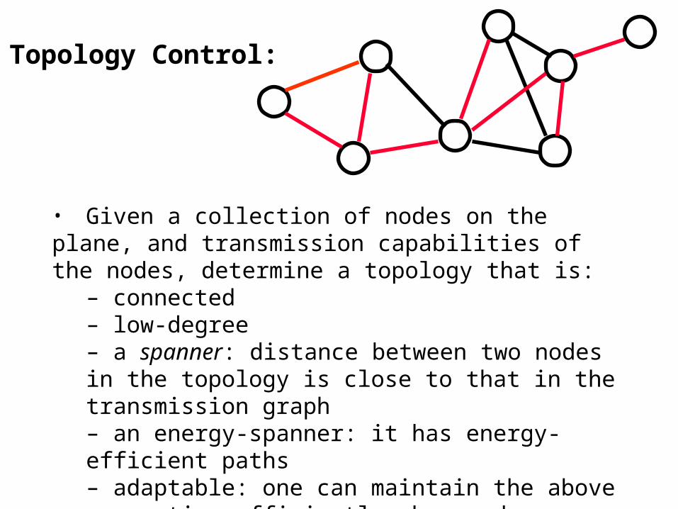
Topology Control:

• Given a collection of nodes on the plane, and transmission capabilities of the nodes, determine a topology that is:

– connected– low-degree– a spanner: distance between two nodes in the topology is close to that in the transmission graph– an energy-spanner: it has energy-efficient paths– adaptable: one can maintain the above properties efficiently when nodes move

Spanning Trees:

K-Dominating Sets:

• useful for routing• single point of failure• non-minimal routes• many variants

• defines partition of the network into zones 1-dominating set

Clustering:

Hierarchical Clustering

• disjoint or overlapping• flat or hierarchical• internal and border nodes and edges Flat Clustering

Basic Routing Schemes

• Proactive Routing: - “keep routing information current at all times”

- good for static networks

- examples: distance vector (DV), link state (LS) algorithms

• Reactive Routing: - “find a route to the destination only after a request comes in”

- good for more dynamic networks

- examples: AODV, dynamic source routing (DSR), TORA

• Hybrid Schemes: - “keep some information current”

- example: Zone Routing Protocol (ZRP)

- example: Use spanning trees for non-optimal routing

Proactive Routing (Distance Vector)

• Each node maintains distance to every other node

• Updated between neighbors using Bellman-Ford

• bits space requirement

• Single edge/node failure may require most nodes to change most of their entries

• Slow updates

• Temporary loops half ofthe nodes

half ofthe nodes

)log( 2 nnO

Reactive Routing - Ad-Hoc On Demand Distance Vector (AODV) [Perkins-Royer 99]- Dynamic Source Routing (DSR) [Johnson-Maltz 96]- Temporally Ordered Routing Algorithm [Park-Corson 97]

• If source does not know path to destination, issues discovery request • DSR caches route to destination• Easier to avoid routing loops

source

destination

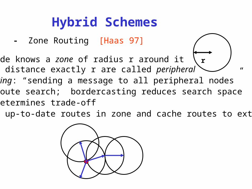
Hybrid Schemes - Zone Routing [Haas 97]

• every node knows a zone of radius r around it• nodes at distance exactly r are called peripheral• bordercasting: “sending a message to all peripheral nodes”• global route search; bordercasting reduces search space • radius determines trade-off• maintain up-to-date routes in zone and cache routes to external nodes

r

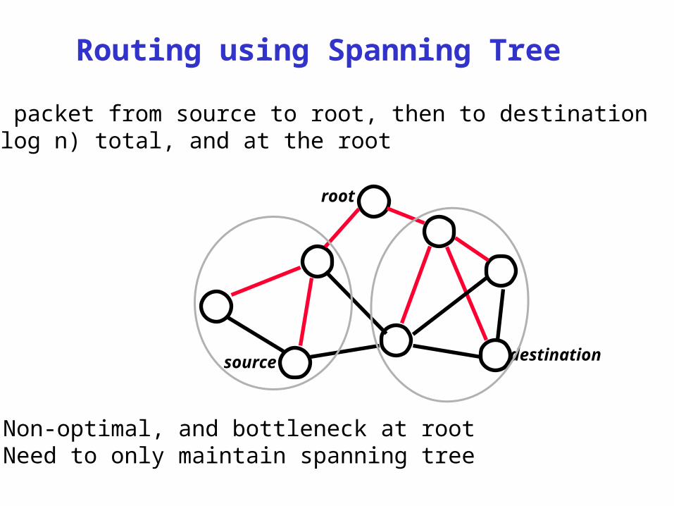
Routing using Spanning Tree

• Send packet from source to root, then to destination• O(n log n) total, and at the root

source

root

destination

• Non-optimal, and bottleneck at root• Need to only maintain spanning tree

Routing by Clustering

• Gateway nodes maintain routes within cluster• Routing among gateway nodes along a spanning tree or using DV/LS algorithms

• Hierarchical clustering (e.g., [Lauer 86, Ramanathan-Steenstrup 98])

Routing by One-Level Clustering[Baker-Ephremedis 81]

Hierarchical Routing

• The nodes organize themselves into a hierarchy• The hierarchy imposes a natural addressing

scheme• Quasi-hierarchical routing: Each node maintains

– next hop node on a path to every other level-j cluster within its level-(j+1) ancestral cluster

• Strict-hierarchical routing: Each node maintains– next level-j cluster on a path to every other level-j

cluster within its level-(j+1) ancestral cluster

– boundary level-j clusters in its level-(j+1) clusters and their neighboring clusters

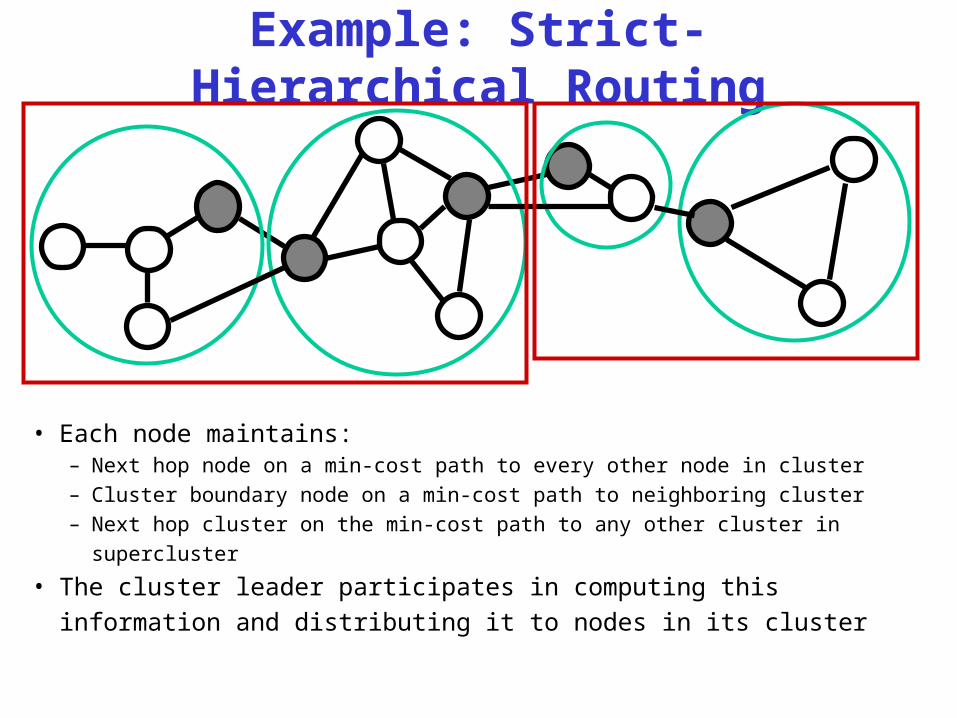
Example: Strict-Hierarchical Routing

• Each node maintains:– Next hop node on a min-cost path to every other node in cluster– Cluster boundary node on a min-cost path to neighboring cluster– Next hop cluster on the min-cost path to any other cluster in supercluster

• The cluster leader participates in computing this information and

distributing it to nodes in its cluster

Space Requirements and Adaptability

• Each node has entries– is the number of levels

– is the maximum, over all j, of the number of level-j clusters in a level-(j+1) cluster

• If the clustering is regular, number of entries per node is

• Restructuring the hierarchy:– Cluster leaders split/merge clusters while maintaining

size bounds (O(1) gap between upper and lower bounds)

– Sometimes need to generate new addresses

– Need location management (name-to-address map)

)(mCOm

C

)( /1 mmnO

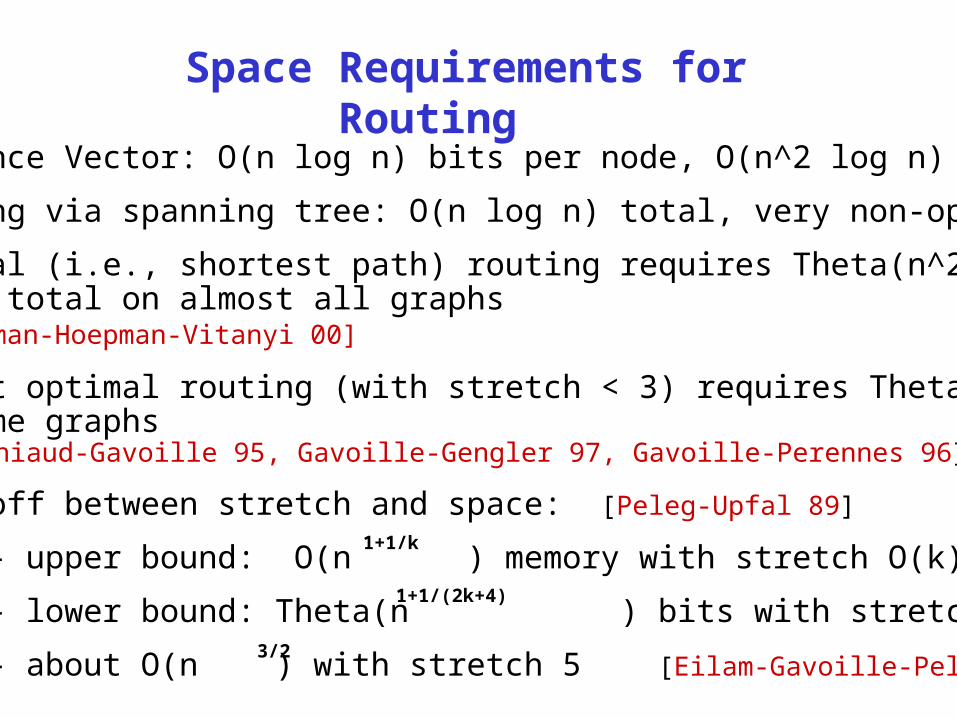
Space Requirements for Routing

• Distance Vector: O(n log n) bits per node, O(n^2 log n) total

• Routing via spanning tree: O(n log n) total, very non-optimal

• Optimal (i.e., shortest path) routing requires Theta(n^2) bits total on almost all graphs [Buhrman-Hoepman-Vitanyi 00]

• Almost optimal routing (with stretch < 3) requires Theta(n^2) on some graphs [Fraigniaud-Gavoille 95, Gavoille-Gengler 97, Gavoille-Perennes 96]

• Tradeoff between stretch and space: [Peleg-Upfal 89]

- upper bound: O(n ) memory with stretch O(k)

- lower bound: Theta(n ) bits with stretch O(k)

- about O(n ) with stretch 5 [Eilam-Gavoille-Peleg 00]

1+1/k

1+1/(2k+4)

3/2

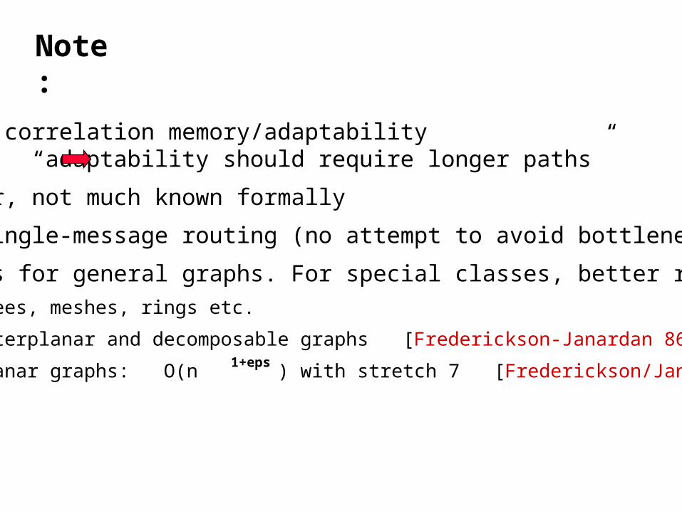
• Recall correlation memory/adaptability “adaptability should require longer paths”

• However, not much known formally

• Only single-message routing (no attempt to avoid bottlenecks)

• Results for general graphs. For special classes, better results:

- trees, meshes, rings etc.

- outerplanar and decomposable graphs [Frederickson-Janardan 86]

- planar graphs: O(n ) with stretch 7 [Frederickson/Janardan 86]

Note:

1+eps

Location Management

• A name-to-address mapping service• Centralized approach: Use redundant location

managers that store map– Updating costs is high– Searching cost is relatively low

• Cluster-based approach: Use hierarchical clustering to organize location information– Location manager in a cluster stores address mappings

for nodes within the cluster– Mapping request progressively moves up the cluster

until address resolved

• Common issues with data location in P2P systems

Content- and Location-Addressable Routing

• how do we identify nodes? - every node has an ID

• are the IDs fixed or can they be changed?

• Why would a node want to send a message to node 0106541 ? (instead of sending to a node containing a given item or a node in a given area)

source

destination 0105641

destination (3,3)

Geographical Routing• Use of geography to achieve scalability

– Proactive algorithms need to maintain state proportional to number of nodes

– Reactive algorithms, with aggressive caching, also stores large state information at some nodes

• Nodes only maintain information about local neighborhoods– Requires reasonably accurate geographic positioning

systems (GPS)– Assume bidirectional radio reachability

• Example protocols:– Location-Aided Routing [Ko-Vaidya 98], Routing in the

Plane [Hassin-Peleg 96], GPSR [Karp-Kung 00]

Greedy Perimeter Stateless Routing

• GPSR [Karp-Kung 00]

• Greedy forwarding– Forward to neighbor closest to destination– Need to know the position of the destination

DS

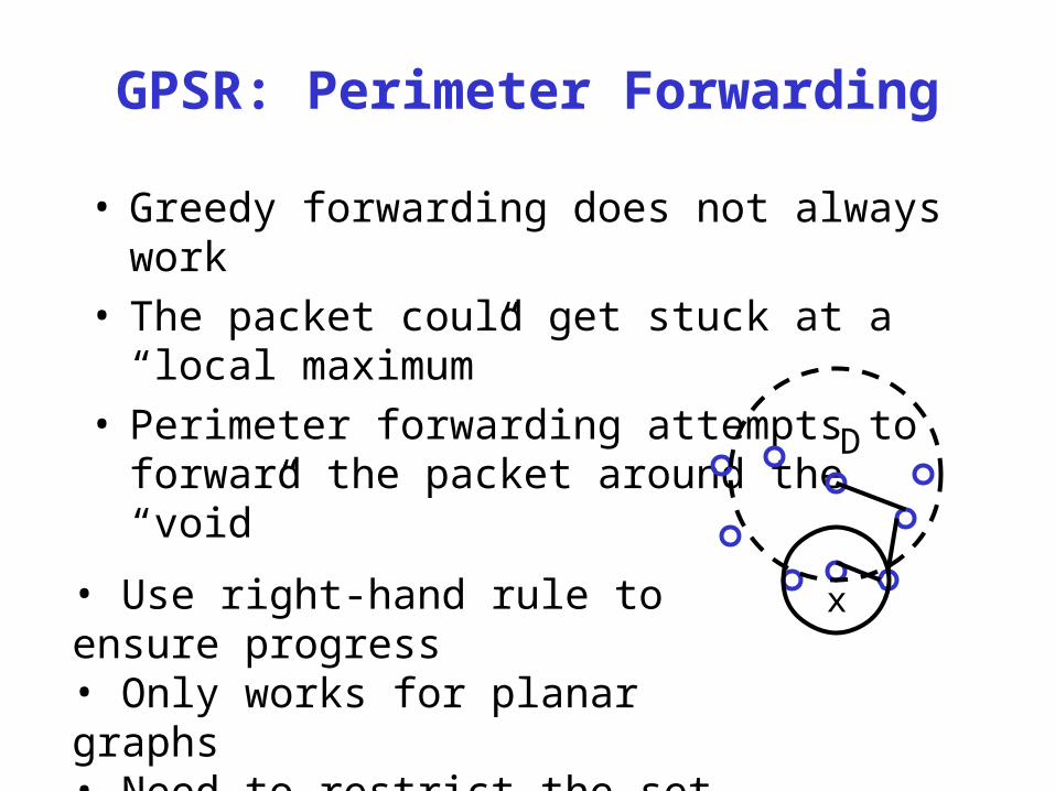
GPSR: Perimeter Forwarding

• Greedy forwarding does not always work• The packet could get stuck at a “local maximum”• Perimeter forwarding attempts to forward the

packet around the “void”

D

x• Use right-hand rule to ensure progress• Only works for planar graphs• Need to restrict the set of edges used

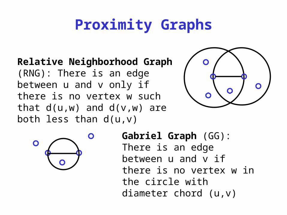
Proximity Graphs

Relative Neighborhood Graph (RNG): There is an edge between u and v only if there is no vertex w such that d(u,w) and d(v,w) are both less than d(u,v)

Gabriel Graph (GG): There is an edge between u and v if there is no vertex w in the circle with diameter chord (u,v)

Proximity Graphs and GPSR

• Use greedy forwarding on the entire graph• When greedy forwarding reaches a local

maximum, switch to perimeter forwarding – Operate on planar subgraph (RNG or GG, for example) – Forward it along a face intersecting line to destination – Can switch to greedy forwarding after recovering from

local maximum

• Distance and number of hops traversed could be much more than optimal

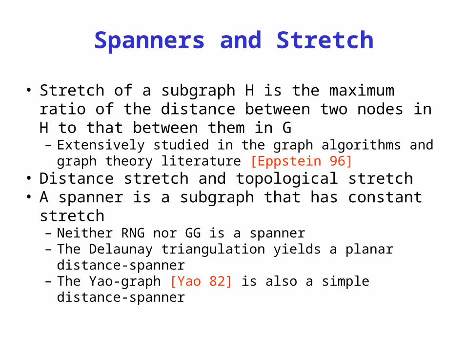
Spanners and Stretch

• Stretch of a subgraph H is the maximum ratio of the distance between two nodes in H to that between them in G– Extensively studied in the graph algorithms and graph

theory literature [Eppstein 96]• Distance stretch and topological stretch• A spanner is a subgraph that has constant stretch

– Neither RNG nor GG is a spanner– The Delaunay triangulation yields a planar distance-spanner– The Yao-graph [Yao 82] is also a simple distance-spanner

Energy Consumption & Power Control

• Commonly adopted power attenuation model:– is between 2 and 4

• Assuming uniform threshold for reception power and interference/noise levels, energy consumed for transmitting from to needs to be proportional to

• Power control: Radios have the capability to adjust their power levels so as to reach destination with desired fidelity

• Energy consumed along a path is simply the sum of the transmission energies along the path links

• Define energy-stretch analogous to distance-stretch

distancepowerTransmit

Power Received

u v ),( vud

Energy-Aware Routing• A path with many short hops consumes less energy than a

path with a few large hops– Which edges to use? (Considered in topology control)– Can maintain “energy cost” information to find minimum-energy

paths [Rodoplu-Meng 98]

• Routing to maximize network lifetime [Chang-Tassiulas 99]– Formulate the selection of paths and power levels as an optimization

problem– Suggests the use of multiple routes between a given source-

destination pair to balance energy consumption

• Energy consumption also depends on transmission rate– Schedule transmissions lazily [Prabhakar et al 2001]– Can split traffic among multiple routes at reduced rate [Shah-Rabaey

02]

Topology Control

• Given:– A collection of nodes in the plane– Transmission range of the nodes (assumed

equal)

• Goal: To determine a subgraph of the transmission graph G that is– Connected – Low-degree– Small stretch, hop-stretch, and power-stretch

The Yao Graph

• Divide the space around each node into sectors (cones) of angle

• Each node has an edge to nearest node in each sector• Number of edges is

• For any edge (u,v) in transmission graph– There exists edge (u,w) in same sector such that w is closer to v than u is

• Has stretch ))2/sin(21/(1

)(nO

u

wv

Variants of the Yao Graph• Linear number of edges, yet not constant-degree• Can derive a constant-degree subgraph by a phase

of edge removal [Wattenhofer et al 00, Li et al 01]– Increases stretch by a constant factor

– Need to process edges in a coordinated order

• YY graph [Wang-Li 01]– Mark nearest neighbors as before

– Edge (u,v) added if u is nearest node in sector such that u marked v

– Has O(1) energy-stretch [Jia-R-Scheideler 02]

– Is the YY graph also a distance-spanner?

Restricted Delaunay Graph• RDG [Gao et al 01]

– Use subset of edges from the Delaunay triangulation

– Spanner (O(1) distance-stretch); constructible locally

– Not constant-degree, but planar and linear # edges

• Used RDG on clusterheads to reduce degree

Spanners and Geographic Routing

• Spanners guarantee existence of short or energy-efficient paths– For some graphs (e.g., Yao graph) easy to construct

– Can use greedy and perimeter forwarding (GPSR)

– Shortest-path routing on spanner subgraph

• Properties of greedy and perimeter forwarding [Gao et al 01] for graphs with “constant density”– If greedy forwarding does not reach local maximum,

then -hop path found, where is optimal

– If there is a “perimeter path” of hops, then -hop path found

)( 2O

)( 2O

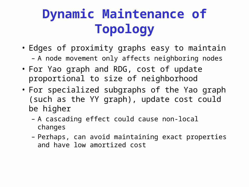
Dynamic Maintenance of Topology

• Edges of proximity graphs easy to maintain– A node movement only affects neighboring nodes

• For Yao graph and RDG, cost of update proportional to size of neighborhood

• For specialized subgraphs of the Yao graph (such as the YY graph), update cost could be higher– A cascading effect could cause non-local changes

– Perhaps, can avoid maintaining exact properties and have low amortized cost

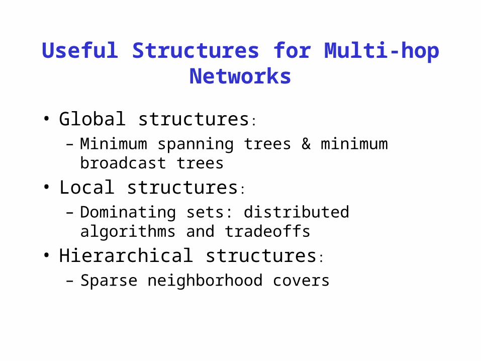
Useful Structures for Multi-hop Networks

• Global structures:

– Minimum spanning trees & minimum broadcast trees

• Local structures:

– Dominating sets: distributed algorithms and tradeoffs

• Hierarchical structures:

– Sparse neighborhood covers

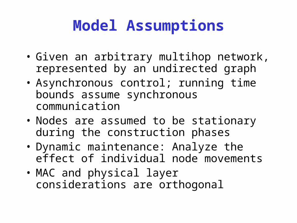
Model Assumptions

• Given an arbitrary multihop network, represented by an undirected graph

• Asynchronous control; running time bounds assume synchronous communication

• Nodes are assumed to be stationary during the construction phases

• Dynamic maintenance: Analyze the effect of individual node movements

• MAC and physical layer considerations are orthogonal

Applications of Spanning Trees

• Forms a backbone for routing• Forms the basis for certain network partitioning

techniques• Subtrees of a spanning tree may be useful during

the construction of local structures• Provides a communication framework for global

computation and broadcasts

Arbitrary Spanning Trees

• A designated node starts the “flooding” process

• When a node receives a message, it forwards it to its neighbors the first time

• Maintain sequence numbers to differentiate between different ST computations

• Nodes can operate asynchronously• Number of messages is ;worst-case

time, for synchronous control, is )(mO

))(Diam( GO

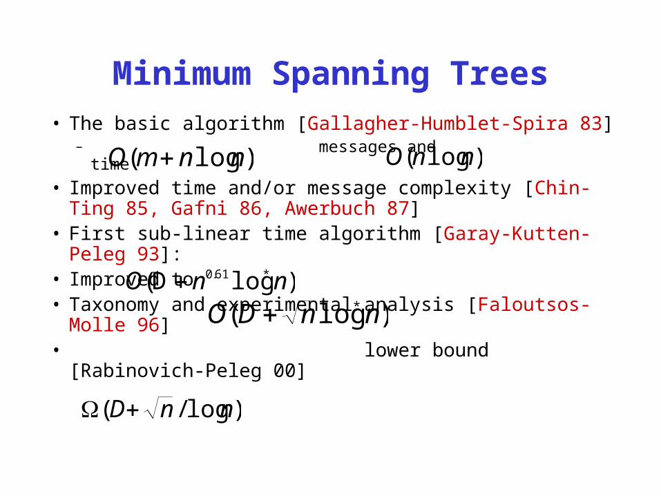
Minimum Spanning Trees

• The basic algorithm [Gallagher-Humblet-Spira 83]– messages and time

• Improved time and/or message complexity [Chin-Ting 85, Gafni 86, Awerbuch 87]

• First sub-linear time algorithm [Garay-Kutten-Peleg 93]:

• Improved to • Taxonomy and experimental analysis [Faloutsos-

Molle 96]• lower bound [Rabinovich-Peleg 00]

)log( nnmO )log( nnO

)logD( *61.0 nnO

)log/( nnD

)log( * nnDO

The Basic Algorithm• Distributed implementation of Borouvka’s

algorithm [Borouvka 26]• Each node is initially a fragment• Fragment repeatedly finds a min-weight edge

leaving it and attempts to merge with the neighboring fragment, say – If fragment also chooses the same edge, then merge

– Otherwise, we have a sequence of fragments, which together form a fragment

1F

2F

2F

Subtleties in the Basic Algorithm

• All nodes operate asynchronously• When two fragments are merged, we should

“relabel” the smaller fragment.• Maintain a level for each fragment and ensure that

fragment with smaller level is relabeled:– When fragments of same level merge, level increases;

otherwise, level equals larger of the two levels

• Inefficiency: A large fragment of small level may merge with many small fragments of larger levels

Asymptotic Improvements to the Basic Algorithm

• The fragment level is set to log of the fragment size [Chin-Ting 85, Gafni 85]– Reduces running time to

• Improved by ensuring that computation in level fragment is blocked for time– Reduces running time to

)log( * nnO

)(nO

)2( O

Level 1 Level 1

Level 2

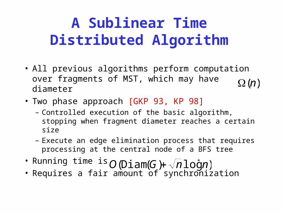
A Sublinear Time Distributed Algorithm

• All previous algorithms perform computation over fragments of MST, which may have diameter

• Two phase approach [GKP 93, KP 98]– Controlled execution of the basic algorithm, stopping

when fragment diameter reaches a certain size

– Execute an edge elimination process that requires processing at the central node of a BFS tree

• Running time is • Requires a fair amount of synchronization

)log)(Diam( * nnGO

)(n

Minimum Energy Broadcast Routing

• Given a set of nodes in the plane, need to broadcast from a source to other nodes

• In a single step, a node may broadcast within a range by appropriately adjusting transmit power

• Energy consumed by a broadcast over range is proportional to

• Problem: Compute the sequence of broadcast steps that consume minimum total energy– Optimum structure is a directed tree rooted at the source

rr

Energy-Efficient Broadcast Trees

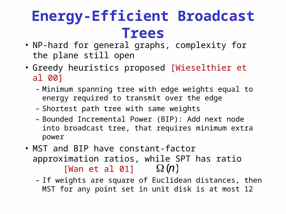
• NP-hard for general graphs, complexity for the plane still open

• Greedy heuristics proposed [Wieselthier et al 00]– Minimum spanning tree with edge weights equal to

energy required to transmit over the edge

– Shortest path tree with same weights

– Bounded Incremental Power (BIP): Add next node into broadcast tree, that requires minimum extra power

• MST and BIP have constant-factor approximation ratios, while SPT has ratio [Wan et al 01]– If weights are square of Euclidean distances, then MST

for any point set in unit disk is at most 12

)(n

• A dominating set of is a subset of such that for each , either– , or– there exists , s.t. .

• A -dominating set is a subset such that each node is within hops of a node in .

Dominating Sets

),( EVG D

DvDu Evu ),(

VVv

k Dk D

Applications

• Facility location– A set of -dominating centers can be selected to locate

servers or copies of a distributed directory– Dominating sets can serve as location database for

storing routing information in ad hoc networks [Liang Haas 00]

• Used in distributed construction of minimum spanning tree [Kutten-Peleg 98]

k

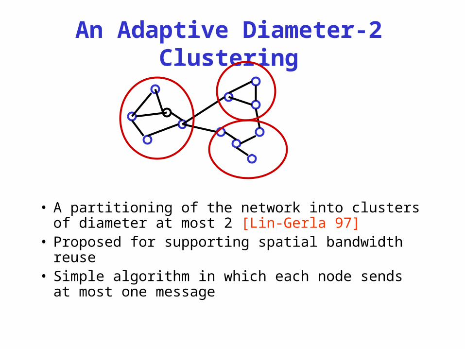
An Adaptive Diameter-2 Clustering

• A partitioning of the network into clusters of diameter at most 2 [Lin-Gerla 97]

• Proposed for supporting spatial bandwidth reuse• Simple algorithm in which each node sends at

most one message

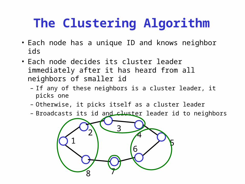
The Clustering Algorithm

• Each node has a unique ID and knows neighbor ids• Each node decides its cluster leader immediately

after it has heard from all neighbors of smaller id– If any of these neighbors is a cluster leader, it picks one

– Otherwise, it picks itself as a cluster leader

– Broadcasts its id and cluster leader id to neighbors

12 3

45

6

78

Properties of the Clustering

• Each node sends at most one message– A node u sends a message only when it has decided its

cluster leader

• The running time of the algorithm is O(Diam(G))• The cluster centers together form a 2-dominating set• The best upper bound on the number of clusters is

O(V)

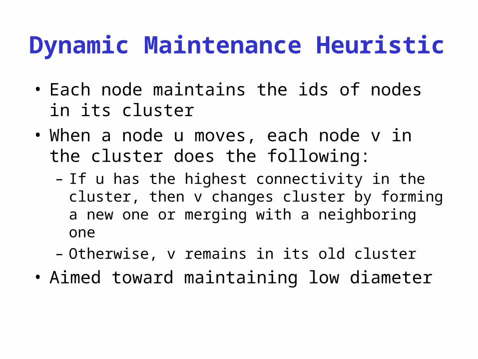
Dynamic Maintenance Heuristic

• Each node maintains the ids of nodes in its cluster• When a node u moves, each node v in the cluster

does the following:– If u has the highest connectivity in the cluster, then v

changes cluster by forming a new one or merging with a neighboring one

– Otherwise, v remains in its old cluster

• Aimed toward maintaining low diameter

The Minimum Dominating Set Problem

• NP-hard for general graphs• Admits a PTAS for planar graphs [Baker 94]• Reduces to the minimum set cover problem• The best possible poly-time approximation ratio

(to within a lower order additive term) for MSC and MDS, unless NP has -time deterministic algorithms [Feige’96]

• A simple greedy algorithm achieves approximation ratio, is 1 plus the maximum degree [Johnson 74, Chvatal 79]

)(log OH

)log(log nOn

• An Example

Greedy Algorithm

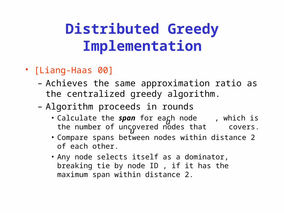
Distributed Greedy Implementation

• [Liang-Haas 00] – Achieves the same approximation ratio as the

centralized greedy algorithm.

– Algorithm proceeds in rounds• Calculate the span for each node , which is the number of

uncovered nodes that covers.

• Compare spans between nodes within distance 2 of each other.

• Any node selects itself as a dominator, breaking tie by node ID , if it has the maximum span within distance 2.

uu

Distributed Greedy

Span Calculation – Round 1

2

2

5

5

3

3

4

4 3

3

Distributed Greedy

Candidate selection – Round 1

2

2

5

5

3

3

4

4 3

3

Distributed Greedy

Dominator selection – Round 1

Distributed Greedy

Span calculation – Round 2

2

2

3

4 3

3

Distributed Greedy

Candidate selection – Round 2

2

2

3

4 3

3

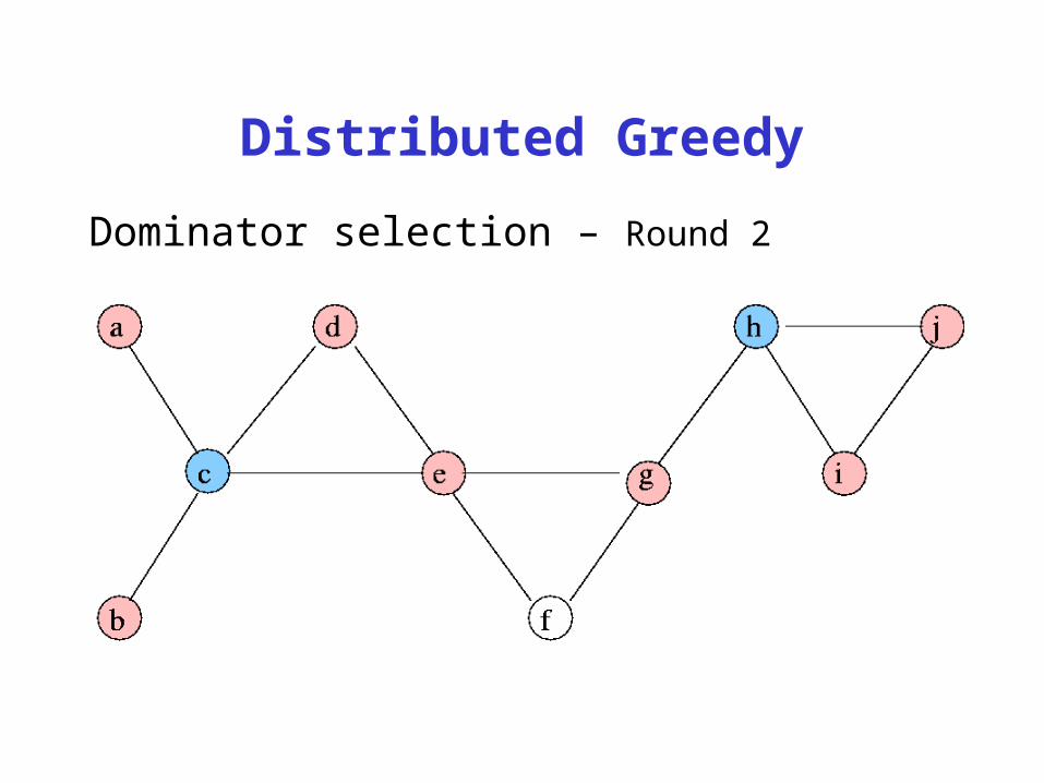
Distributed Greedy

Dominator selection – Round 2

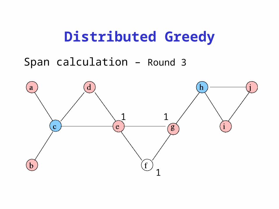
Distributed Greedy

Span calculation – Round 3

1

1 1

Distributed Greedy

Candidate selection – Round 3

1

1 1

Distributed Greedy

Dominator selection – Round 3

Lower Bound on Running Time of Distributed Greedy

Running time is for the “caterpillar graph”, which has a chain of nodes with decreasing span.

)( n

Simply “rounding up” span is a cure for the caterpillar graph, but problem still exists as in the right graph, which takes running time .

)(n

Faster Algorithms

• -dominating set algorithm [Kutten-Peleg 98]

–Running time is on any network.–Bound on DS is an absolute bound, not relative to the optimal result.– -approximation in worst case. – Uses distributed construction of MIS and spanning forests

• A local randomized greedy algorithm, LRG [Jia-R-Suel 01]

– Computes an size DS in time with high probability– Generalizes to weighted case and multiple coverage

k

)(log* nO

)(n

)(lognO )(log2 nO

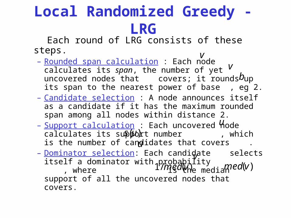
Local Randomized Greedy - LRG Each round of LRG consists of these steps.

– Rounded span calculation : Each node calculates its span, the number of yet uncovered nodes that covers; it rounds up its span to the nearest power of base , eg 2.

– Candidate selection : A node announces itself as a candidate if it has the maximum rounded span among all nodes within distance 2.

– Support calculation : Each uncovered node calculates its support number , which is the number of candidates that covers .

– Dominator selection: Each candidate selects itself a dominator with probability , where is the median support of all the uncovered nodes that covers.

u

vv

b

)(us

)(/1 vmed )(vmed

uv

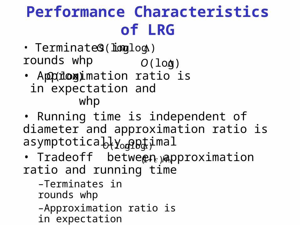
Performance Characteristics of LRG

• Terminates in rounds whp• Approximation ratio is in expectation and whp • Running time is independent of diameter and approximation ratio is asymptotically optimal• Tradeoff between approximation ratio and running time

–Terminates in rounds whp–Approximation ratio is in expectation

• In experiments, for a random layout on the plane:– Distributed greedy performs slightly better

)log(log nO

)(logO)(log nO

)log(log nO

H)1(

Hierarchical Network Decomposition

• Sparse neighborhood covers [Awerbuch-Peleg 89, Linial-Saks 92]– Applications in location management, replicated data

management, routing

– Provable guarantees, though difficult to adapt to a dynamic environment

• Routing scheme using hierarchical partitioning [Dolev et al 95]– Adaptive to topology changes

– Week guarantees in terms of stretch and memory per node

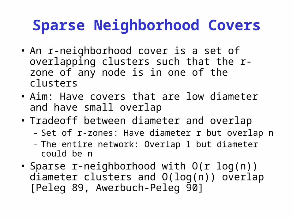
Sparse Neighborhood Covers

• An r-neighborhood cover is a set of overlapping clusters such that the r-zone of any node is in one of the clusters

• Aim: Have covers that are low diameter and have small overlap

• Tradeoff between diameter and overlap– Set of r-zones: Have diameter r but overlap n– The entire network: Overlap 1 but diameter could be n

• Sparse r-neighborhood with O(r log(n)) diameter clusters and O(log(n)) overlap [Peleg 89, Awerbuch-Peleg 90]

Sparse Neighborhood Covers

• Set of sparse neighborhood covers– { -neighborhood cover: }

• For each node:– For any , the -zone is contained within a cluster

of diameter – The node is in clusters

• Applications:– Tracking mobile users– Distributed directories for replicated objects

r)log( nrO

)(log2 nO

ni log0

r

i2

Online Tracking of Mobile Users

• Given a fixed network with mobile users• Need to support location query operations• Home location register (HLR) approach:

– Whenever a user moves, corresponding HLR is updated

– Inefficient if user is near the seeker, yet HLR is far

• Performance issues:– Cost of query: ratio with “distance” between source and

destination

– Cost of updating the data structure when a user moves

Mobile User Tracking: Initial Setup

• The sparse -neighborhood cover forms a regional directory at level

• At level , each node u selects a home cluster that contains the -zone of u

• Each cluster has a leader node.

• Initially, each user registers its location with the home cluster leader at each of the levels

i2i

)(lognO

i2i

The Location Update Operation

• When a user X moves, X leaves a forwarding pointer at the previous host.

• User X updates its location at only a subset of home cluster leaders– For every sequence of moves that add up to a

distance of at least , X updates its location with the leader at level

• Amortized cost of an update is for a sequence of moves totaling distance

i2i

)log( ndOd

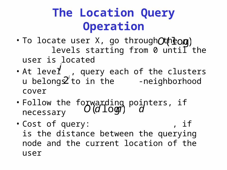
The Location Query Operation

• To locate user X, go through the levels starting from 0 until the user is located

• At level , query each of the clusters u belongs to in the -neighborhood cover

• Follow the forwarding pointers, if necessary

• Cost of query: , if is the distance between the querying node and the current location of the user

i2i

)log( ndO d

)(lognO

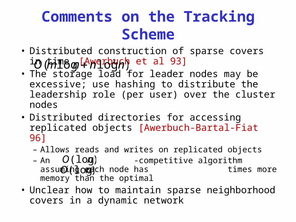
Comments on the Tracking Scheme

• Distributed construction of sparse covers in time [Awerbuch et al 93]

• The storage load for leader nodes may be excessive; use hashing to distribute the leadership role (per user) over the cluster nodes

• Distributed directories for accessing replicated objects [Awerbuch-Bartal-Fiat 96]– Allows reads and writes on replicated objects– An -competitive algorithm assuming each node

has times more memory than the optimal

• Unclear how to maintain sparse neighborhood covers in a dynamic network

)loglog( 2 nnnmO

)(lognO)(lognO

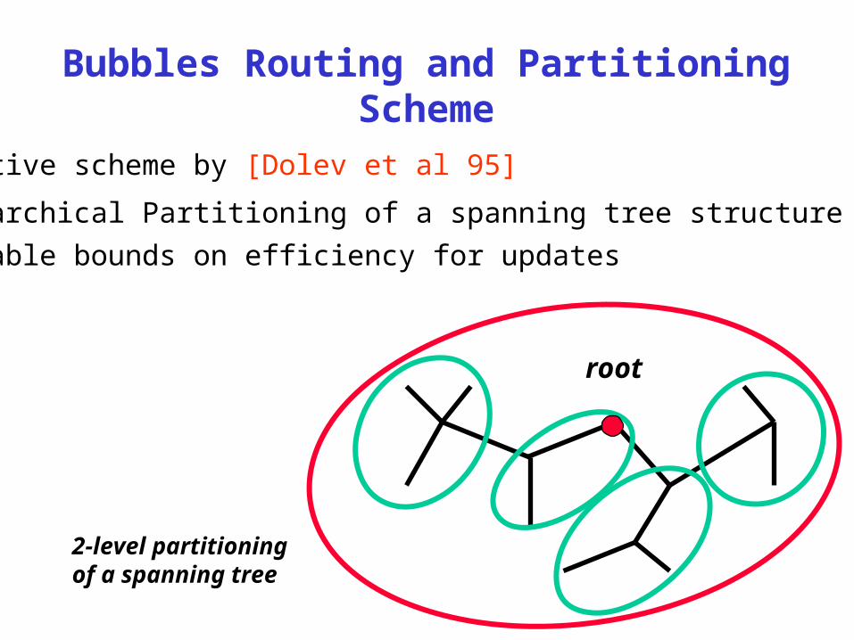
Bubbles Routing and Partitioning Scheme

• Adaptive scheme by [Dolev et al 95]

• Hierarchical Partitioning of a spanning tree structure

• Provable bounds on efficiency for updates

2-level partitioningof a spanning tree

root

Bubbles (cont.)

• Size of clusters at each level is bounded

• Cluster size grows exponentially

• # of levels equal to # of routing hops

• Tradeoff between number of routing hops and update costs

• Each cluster has a leader who has routing information

• General idea:

- route up the tree until in the same cluster as destination,

- then route down

- maintain by rebuilding/fixing things locally inside subtrees

Bubbles Algorithm

• A partition is an [x,y]-partition if all its clusters are of size between x and y

• A partition P is a refinement of another partition P’ if each cluster in P is contained in some cluster of P’.

• An (x_1, x_2, …, x_k)-hierarchical partitioning is a sequence of partitions P_1, P_2, .., P_k such that

- P_i is an [x_i, d x_i] partitioning (d is the degree)

- P_i is a refinement of P_(i-1)

• Choose x_(k+1) = 1 and x_i = x_(i+1) n1/k

Clustering Construction

• Build a spanning tree, say, using BFS

• Let P_1 be the cluster consisting of the entire tree

• Partition P_1 into clusters, resulting in P_2

• Recursively partition each cluster

• Maintenance rules:

- when a new node is added, try to include in existing cluster, else split cluster

- when a node is removed, if necessary combine clusters

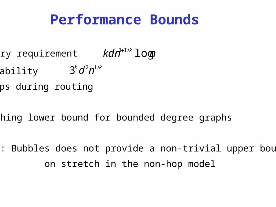
• memory requirement

• adaptability

• k hops during routing

• matching lower bound for bounded degree graphs

• Note: Bubbles does not provide a non-trivial upper bound

on stretch in the non-hop model

Performance Bounds

kk nd /123

nkdn k log/11