RD-Ri21 817 DISEASE MODELLING OF JAPANESE ENCEPHALITIS IN TAIWAN i/THROUGH THE USE OF SATELLITE REMOTE SENSING(U) EARTHSATELLITE CORP CHEVY CHASE MD C SHEFFIELD 36 AUG 92

UNCLASSIFIED N9814-8i-C-7i2 F/G 65 ,N

1.

,-:: .... III 1.0 llW 2

ii.2

.6 -

lio5111.6

MICROCOPY RESOLUTION TEST CHARTmAoO..a&. ounta& Or STALPMI - 194 A

DIEASE MODEING OF JAPANESE ENCEPHALUS IN TAIWANTHROUGH THE USE OF SATELT RMOTE SENSING

C

, u u ..,S NOV 2 419T

Prpr e for

THE NAVAL MEICAL mnA INTul4U.S. NATIONAL NAVAL MEDICAL CENTER E

Under Contrat N0001441,C0712 _

Aupst 30, 1982

11Sdif'Ltunt has beou approvedfafpL)jj ri (I; id Palo, it EARTH SATELLITE CORPORATION Ethij

dlbut s rrdo Chevy Chase, Marylan, USA(Eth )[ 8 1117 014

TECHNICAL REPORT STANOARD TITLE PAGE

I Relert N. 12. Government Accession N . ' 3. Recipient's Catalog No.

'4 ite & nd Subtitle 1 5. Report Dot*Disease Modelling of Japanese Encephalitis August 30, 1982

in Taiwan Through the Use of Satellite Remote 6. Performing organization CodeSensing7. Author(s) 8. Performing Organization Report No.Charles Sheffield9. Performing Organization Name and Address 10. Work Unit No.

Earth Satellite Corporation7222 47th Street 11. Contract or Grant Ne.

Chevy Chase, Maryland 20815 N00014-81-C-071213. Type of Report and Period Covered

12. Sponsoring Agency Home and Addos, Final ReportI September 1981 -Naval Medical Research Institute September 1982(September 1982National Naval Medical Center '14. Sponsoring Agency CodeBethesda, Maryland 20014

15. Supplementary Ntes

16. bstrect

This report describes the development of probability models for theoccurrence of infectious disease using variables derived from theLandsat series of satellites and other geographic factors. The models Uare applied to yield a predictive program for the occurrence ofJapanese encephalitis on the island of Taiwan. Four different formsof model are evaluated: linear regression, log-linear regression, logimodels, and discriminant analysis. Observations consisted of diseasedata from 106 sites in Taiwan, in the period 1968-1975. Of the modelsemployed, it was found that linear regression produces the best result ,and a 9-variable linear regression was preferred. The independentvariables in this case consist of means and variances of Landsat dataover regions surrounding each disease site, plus altitude data. Asignificant correlation was found between observed and predicteddisease incidence rates (correlation coefficient = 0.75). No system-atic residual biases were observed in the final predicted results.The overall form of the model and the use of the data should remainthe same for many infectious diseases in many different parts of theworld.

17. Key Woerds(S lected by Auther(s)) 18, Distribution Stetement

Japanesel encephalitis, Landsat,infectious disease, statisticalmodel, remote sensing, Taiwan.

119. Security Clessif. (of this repert) 120. Security Classi. (of this page) 121. Me. of Pages 122. Price*

Unclassified Unclassified 60

"]Foe sale by the Cleariagouse for Federal Scientific and Technical Informsion, Springfield. Virginis 22151.

I .

FOREWORD AND ACKNOWLEDGEMENTS

This study is the product of a contract (N00014-81-C-0712) funded

by the Office of Naval Research as part of a Naval Medical Research and

Development Command DD 1498 number MF58524.009 entitled "Infectious

Diseases Risk Assessment in Foreign Operations Involving Military Forces."

The Principal Investigator of this work unit is LT Gary Pazzaglia and

the Associate Investigator is Ms. Eleanor Cross. We wish to express

thanks to LCDR James Olson of the Yale Arbovirus Research Unit for supply-

ing the required disease data for Japanese B encephalitis in Taiwan and

to Dr. Charles Barnes of the International Veterinary Medical Foundation

for helping to formulate the conceptual framework for this study.

Appreciation is also given to CDR R. I. Walker of Naval Medical Research

Institute for guidance in overall project design.

Accession For-NTIS - i :

!Dit L I Spi7..7DL-40%

Sod~es

'A kl i L d/or

1. D t secia

GENERAL SUNMARY j

Military operations frequently require the introduction of non-

indigenous personnel to geographic areas for which data on infectious

diseases are absent or unreliable. For many parts of the world, prior

ground or aircraft reconnaissance may also be impossible.

This report addresses the problem of assessing the probability of

infectious disease occurrence using generally available geographic

variables. In particular, variables are employed that utilize data

provided by the Landsat series of satellites, combined with altitude and

location information. A set of statistical models is developed and

applied to the analysis of a particular disease, that of Japanese encepha-

litis occurring on the island of Taiwan.

Following a description of the general characteristics of data

provided by the Landsat satellites, a summary of relevant facts concerning

the etiology of Japanese encephalitis is presented. These facts dictate

the general form of statistical models to be employed in numerical experi-

ments. Four models are applied: linear regression, log-linear regression,

logit models, and discriminant analyses. In each case, observed disease

data for a set of 106 sites in Taiwan for the period 1968 to 1975 constitute

the dependent variables, with independent variables obtained from Landsat,

altitude and location data.

Of the four models employed, it is found that linear regression analysis

offers the most promise. Within the set of linear regression models employed,

a 9-variable form gives the best results. The independent variables in this

preferred case consist of altitudes of disease sites and the means and

variances of Landsat data over square regions surrounding each disease

site location.

Use of this model over sets of Taiwan disease sites leads to a

significant correlation between observed and predicted incidence rates

for Japanese encephalitis. The observed correlation coefficient of 0.75

is insensitive to the particular subset of disease sites used to develop

the model coefficients, and no systematic biases are discernible in the

final predicted results. The etiology of the disease suggests that the

future'inclusion of additional independent variables, in particular weather

variables, might strengthen the correlations.

The results of this work consist of a set of statistical models

whose coefficents must be determined for any particular disease and geo-

graphic region. However, the overall form of the model and the use of

data should remain the same for many infectious diseases, in many different

parts of the world.

TABLE OF CONTENTS

Page

I. INTRODUCTION 1

II. REMOTE SENSING AND THE INFORMATION PROVIDED BY SATELLITECOVERAGE 5

A. The uses of remote sensing and the U.S. EarthResources Program 5

B. The Landsat system 6

III. JAPANESE ENCEPHALITIS AND ITS SUITABILITY TO DISTRIBUTION

MODELLING 10

A. History and etiology of Japanese encephalitis 10

B: Japanese encephalitis data for Taiwan 12

IV. THE STATISTICAL MODELS EMPLOYED IN THE INVESTIGATION 14

A. Selection of models 14

B. The regression analysis model 18

C. Logit models 19

D. Discriminant analysis 22

V. DATA PROCESSING PROCEDURES 24

A. The Landsat data base 24

B. Weather data 27

C. Altitude data and location data 28

D. Determination of the set of independent variables 28

VI. RESULTS OF THE STATISTICAL MODELS 31

A. General comparison of the logit and regressionmodels 31

ii

Page

B. General results of the discriminant analysis 32

C. Results of the regression models and theaddition of other variables 34

D. Other experiments and the summary of results 36

VII. CONCLUSIONS 39

REFERENCES

APPENDIX A: DISEASE STATISTICS

DISEASE MODELLING OF JAPANESE ENCEPHALITIS IN TAIWANTHROUGH THE USE OF SATELLITE REMOTE SENSING

I. INTRODUCTION

Attempts to understand the occurrence and spread of infectious

diseases probably pre-date written history, although scientific ideas on

the subject are of much more recent vintage. The notion of bacterial

action as an immediate physical cause of disease was proposed by Girolamo

Fracastoro more than four hundred years ago, in 1546,1 but its acceptance

awaited Pasteur's and Koch's work in the 1870's.2,3 The idea that insects

might serve as vectors for disease transmission is more recent yet, dating

only from Smith and Reed's work4 ' at the end of the last century.

Although there still remain large gaps in our understanding of the

detailed interactions between hosts and vectors as they govern the

occurrence and propagation of arthropod-borne diseases, we can now feel con-

fident that the following factors are all of great significance in deter-

mining the probability of infection and spread of human disease:

* the sensitivity of both host and vector to climatic andgeographic variations, including habitat, temperature,altitude, landforms, and rainfall;

" the presence or absence of alternate animal hosts thatserve as potential amplifiers for disease occurrence (as,for example, hogs serve as an amplifying factor forJapanese encephalitis);

" the distribution and degree of exposure of the human

population;

" the innate or induced resistance of the human population;

" the prevailing regional cultural practices, e.g., cleanli-ness and sanitation.

-2-

When, as is frequently the case in military operations, a group of

non-indigenous humans is introduced to a region, data on disease occurrence

will often be lacking. The native populations may possess acquired

immunity, or the region may be so sparsely populated that data on diseases

are non-existent, or lack any statistical validity. In many parts of the

world, inadequate reporting systems for disease data are the rule rather

than the exception. There is a definite need for some predictive tool which

can take detailed geographic knowledge of a region and make reasonable esti-

mates as to the disease rates that would be encountered in a non-immune group

enterfng the region.

The biggest impediment to the use of predictive models based on funda-

mental biological interactions is the absence of knowledge of explicit causal

relationships. The physical variables that couple environment, human host,

vector and disease agent are frequently unknown in the necessary detail. How-

ever, in such circumstances, It is always possible to employ a purely statis-

tical model in which relationships are studied empirically and through

statistical correlations. No predictor of this type will offer perfect per-

formance, and there will remain unknown influencing factors. In addition, it

will normally require more data to establish the parameters of a statistical

model than a biologically defined model, since the functional form of the

latter is known from the biology, whereas the former must rely on the data to

define both the form and the unknown constants of the model. On the positive

side, an established statistical correlation can often suggest a productive

approach to deterministic models based more on causal relationships.

-3-

All statistical models are inherently data dependent. Thus in military

operations a further complication arises when areas are inaccessible to ground

investigation or to aircraft overflight. In practice, these areas may also

be those of greatest military interest.

In such circumstances, data acquired remotely by artificial satellites

can often provide the detailed overview needed for disease distribution models,

defining the necessary land use, geography, ground cover and topography. Such

data can be obtained regularly throughout the year, without a ground or air-

craft presence, and represent a powerful new potential for disease distribution.." modelli'ng.

In this report, the first steps are taken towards a distribution model

for infectious diseases that is minimally dependent on ground presence or air-

craft overflights. The first application has been to a particular disease in

a particular location (Japanese encephalitis on the island of Taiwan) but the

principles employed are quite general, and the supporting satellite data base

is available anywhere in the world.

The organization of the report is as follows:

Section I - Introduction: Background on the modelling ofinfectious diseases, and the governing variablesthat apply.

Section II - Remote sensing and the information provided bysatellite coverage: An overview of the Landsatprogram and the data provided by it.

Section III - Japanese encephalitis and its suitability todistribution modelling: A summary of studiesperformed to date of the disease and the factorsthat appear relevant to its propagation.

-I

-4-

Section IV The statistical models employed in the investiga-tion: Logit models, regression analysis,discriminant analysis, and their application todisease models.

Section V The data base and the statistical processing:Manipulation of the Landsat data base, image window-ing, spectral band combinations, and the additionof topographic variables.

Section VI - Results of the investigation

Section VII - Conclusions

References

-5-

II. REMOTE SENSING AND THE INFORMATION PROVIDED BY SATELLITE COVERAGE

A. The uses of remote sensing and the U.S. Earth Resources

Program

The idea that information useful for natural science investiga-

tions might be obtained from satellites arose as a natural extension of the

use of aerial photographs in the first half of this century. Early experi-

ments using balloon-borne cameras for monochrome photography in the 1850's6

led to the use of aerial photography for survey purposes in the 1920's

In the Second World War, the power of infrared film to distinguish camouflage

from healthy growing vegetation began the use of wavelengths beyond the

visible,8 and in the 1960's handheld cameras aboard the Gemini and Apollo

spacecraft showed the power of photographic coverage of a very large area.

It was therefore natural, when a series of satellites for the measure-

ment of the Earth's resources was conceived in the late 1960's, that multiple

uses of the data would be attempted. The initial list of roughly 350 experi-

ments approved by NASA in 1972 for the first such satellite (known originally

as ERTS-l and later as Landsat-l) covered numerous disciplines and application

areas.9 These ranged from practical applications in crop monitoring, geological

mapping, and oil and gas exploration, to experiments aimed at determining the

best manner of presenting the information collected by the spacecraft. There

were even experiments performed for disease monitoring, but they were con-

fined to timber disease, where the effects on growing trees were directly

visible on the images. No experiments for the use of satellite data for human

disease distribution were proposed, perhaps because of the lack of explicit

causal models that could link observable ground features with disease incidences.

However, soon after the launch of Landsat-1, satellite data from the NOAA 2 and

NOAA 3 satellites were used successfully in the U.S./Mexico Screwworm Eradication

-6-

Project in 1973-1975. 10

The satellites of the U.S. Earth Resources Program were not designed

for high-resolution surveillance work, and in fact all the data collected

by the program is unclassified and can be purchased for use by anyone. As

a result, there are practical limitations on the smallest size area that

can be analyzed using such data; as a compensating advantage, very large

areas (more than ten thousand square miles) can be analyzed in a single image.

In addition to the Landsat satellites that provided the main data source

for this project, the United States operates weather service satellites that

give worldwide coverage at visible and thermal infrared wavelengths several

times a day. These satellites offer a less detailed picture than the Landsat

satellites, but have the advantage of more frequent coverage of any particular

ground area.

B. The Landsat system

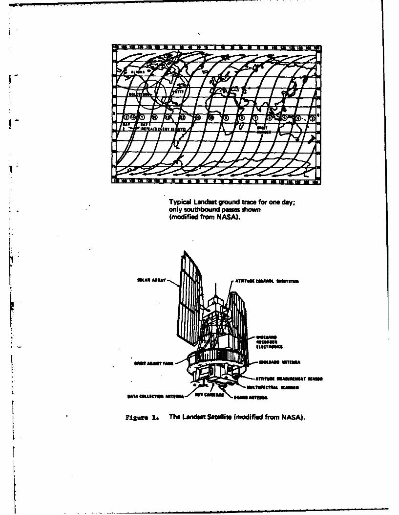
Four Landsat spacecraft have so far been launched, but data from

Landsat-4 (launched July 1982) are not yet available. Landsats-1, -2 and -3

move in sun-synchronous orbits so that each satellite images the Earth at the

same local time of day, about 9:30 a.m. The orbits are close to polar, almost

circular, and have a period of 103 minutes. The satellites travel at an aver-

age height of about 900 kilometers, and each satellite provides complete cover-

age of the Earth's surface in latitudes lower than 810 every 18 days11 (Figure 1).

Landsat-4 occupies a lower orbit with an average height of about 700 kilometers

and provides complete coverage of latitudes lower than 810 every 16 days.

II L

Typical Landut ground trace for one day;only southbound paswe shown(modified from NASA).

MiAN AueAT AMOKui usmue Oww'm

smiw~saui TMS

Figure 1j, The LandM Satellite (modified from NASA).

I

-7-

Cloud cover may diminish the usefulness of acquired data since the

sensing of the Earth's surface takes place only in visible and near-visible

wavelengths which have no cloud penetrating power. This can be a severe

drawback in equatorial regions, where cloud cover is present most of the time.

The primary observing instrument on the first three Landsat spacecraft,

and the one that was used to provide data for this project, is a Multi-Spectral

Scanner (MSS). It senses reflected radiation from the Earth with a field of

view that covers an area 79x79 metres on the Earth's surface. The incident

radiation at the spacecraft is spectrally decomposed in the spacecraft optics

* -to four wavelength regions: 0.5 to 0.6 micrometres (usually termed the

"green band"); 0.6 to 0.7 (the "red band"); 0.7 to 0.8 (the "first infrared

band"); and 0.8 to 1.1 (the "second infrared band"). Successive scan lines

of data are generated by the forward motion of the spacecraft in its orbit.

A complete coverage of a swath of the surface, roughly 185 kilometres wide, is

continuously generated as the spacecraft traverses the daylight side of the

Earth. (Note: The fourth spacecraft in the series, Landsat-4 has a thermal

infrared band that permits night-side sensing also; a similar instrument on

Landsat-3 never returned usable data because of detector malfunction.)

The four spectral bands of data are returned to Earth in two separate

modes. If the spacecraft is in line-of-sight range of a Landsat ground

receiving station, the data are converted to digital form and transmitted

electronically in real-time to the station. If no station is in line-of-

sight range, data my be stored on on-board tape recorders, for subsequent

electronic transmission to a ground station (See Figure 2). During the pro-

cess of transmission to the ground, the signal in each spectral band is

LANOSAT SATELLITE313 KM 1570 MI) ALTITUDE

-" INFORMATION TELEMETERPOTO GROUND STATION EEG

TELEMETERED INFORMATION RECEIVED boi nremgtion n IewteredAT STATION IS PROCIESSED AND STORED to reevn sin an* et

ON VIDEO TAPE ... whe seef is i lio

det i ma saren board until

V setellts is in proxienit of

CONATIMILESOARAITN-

POE irly ff 8" wituft to am

Inkin l(X115 lsugmndbs).BLACK at WHITE IMAGES PRODUCEDFROM TAPES (BULK PRCSSl

IMAGES CAN BE ADDITIONALLYBAND 4 -MODIFIED BY COMPUTER PROCESSING

BULK OR COMPUTER PROCESSED LAtWHITE IMAGES ARE COMBINED TO FORM EACH PIXEL IS EOWJVALENT IN AREA TO

COLORIMAM ev C46 HECTARES 11. 1 ACRES) ON THE GROUNDTHE PI XELS REPRESENT THE "AVERAGE ENVIRONMENT"

-~ - _ _ _ _ _ _ _ _ _ I. E N LA R G EM EN T O F PIX EL

E IAGE CONSVISTS OF 2300 SCAN LINES. 1

EACH SWAN LINE CONTAINS 20 PIXELS

we sin

Figure 2. Sequence of Landsat Information System

-8-

over-sampled to give a ground resolution along the scan-line of 57 metres.

Thus the received digital signal is that of sets of ground areas each 79m x

57m, roughly 1.1 acres, in each of four spectral bands. The digital signal

returned to Earth from the satellite assigns the observed ground reflec-

tances to one of 64 distinct reflectance levels (256 for Landsat-4) that

are usually termed grey levels. The individual distinguishable ground areas

S- are termed picture elements, or pixels.

[ Although the observations made by the scanner are a continuous swath

of data of width 185 kms, for practical use the data stream is arbitrarily

chopped into sections corresponding to squares of 185 km2. This is conven-

tionally termed a Landsat "scene" or "frame." Each such frame contains

roughly 7.6 million pixels. The very large volumes of data that constitute

a single Landsat scene make computer processing mandatory.

Before the information provided by the spacecraft can be used, a number

of geometric and radiometric corrections must be applied. The most obvious

one in terms of the appearance of the reconstructed image is the correction

for Earth rotation, which leads to a rhomboidal rather than a square shape for

a single image frame. However, for practical use of the data, the most

important correction is probably that compensating for variations in detector

sensitivity, which if it occurs, leads to a striped or banded image and strongly

degrades the spectral fidelity of the data. This is a very important factor

in activities such as image classification, or in the statistical analyses

performed on this project.

Landsat data are typically displayed in a standard false color pre-

sentation in which the first infrared band (0.7 to 8.Opm) is not used. This

-9-

is usually justified since there are strong correlations between the

data of the first and second infrared band. However, in this work all

possible statistical strength was desirable, and all experiments employed

all four Landsat spectral bands.

[

-10-

III. JAPANESE ENCEPHALITIS AND ITS SUITABILITY TO DISTRIBUTION MODELLING

A. History and etiology of Japanese encephalitis

The disease now recognized as Japanese encephalitis (JE) and

also as "summer encephalitis" occurs throughout eastern Asia, as far north

as Siberia and as far south as the East Indies from Guam to eastern India.

The disease is characterized by fever, encephalitic symptoms, and a high

mortality rate. It attacks primarily young children during the summer season.

The incidence of the disease correlates with the warm part of the year in

areas to the north of Taiwan, including Okinawa and Japan, and shows much;: 12less correlation with season south of Taiwan. Japanese encephalitis was

first reported in Taiwan by Sakai in 1935, and has been a legally defined

reportable disease by the Taiwan Provincial Health Department since 1955.13

The primary vector for the transmission of JE virus on Taiwan is Culex

tritaeniorhynchus, with C. fuscocephalus as a possible other vector in the

southern part of the island.14 C. tritaeniorthynchus is a mosquito that breeds

in clean water in cultivated fields, and in stable bodies of water around such

fields.15 There is a rapid seasonal increase in the population of the mosquito,

with a peak in July and August, that may be linked to some specific agricultural

practice on the island. However, in India and in Thailand there is some evi-

dence that the population of the adult mosquito may be more influenced by rain-

16fall rather than any type of irrigation practice. In more northern areas,

including Taiwan, mosquito population densities seem to follow the annual

temperature curves, with peak adult population in the summer months.

The disease rates for a human population newly introduced to Taiwan

would probably be quite different from the native population, since they would

* lack any previous exposure to the JE virus. It appears that a large per-

centage of the adult native population is immune as a result of childhood

* infection, often of a subclinical nature.13 Nonetheless, JE was one of

the most important endemic diseases of the island during the period studied.

The development of a suitable JE vaccine and its use from 1976 onwards in

a successful public health program have in recent years much reduced the

prevalence of the disease.

Of the facts cited here, the ones that are of the most significance in

establishing a disease distribution model are thought to be as follows:

S1. The definition of JE as a legally reportable disease

has produced reliable disease statistics for Taiwan. There is

a data base that gives not only incidence rates, but the

specific place of residence associated with each case. This is

unusual, since disease data are commonly aggregated to the point

where specific geographic locations disappear. Since we are

Lseeking to correlate the disease with site-specific geographic

variables, site-specific incidence rates are essential.

2. The vector for JE breeds in particular environments

that should be correlatable with land cover and land use discern-

ible from space imagery.

3. The probable presence of alternate hosts, in particular

the domestic swine, complicates the analysis. Disease foci may

be expected around hog farms, which may or may not be distinguish-

able with the resolution of the data provided by the Landsat

satellites.

-I i maalmllm O ilil m m a[m N ,-- -, ..

-12-

4. Prior infection of the native population will reduce

current disease levels; thus disease incidence rates may reflect

stability of population at one location as much as they indicate

the exposure risk at that location.

B. Japanese encephalitis data for Taiwan

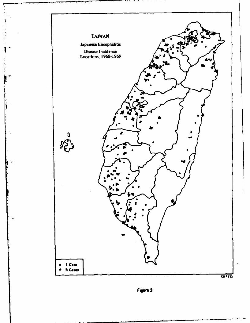
Disease incidence rates for JE in Taiwan were collected by the

Taiwan Provincial Health Department at 106 locations, mainly in the western

part of the island in the period 1968-75. Figure 3 shows the locations of

cases occurring during 1968-69 and is representative of the geographic

distribution of all cases over the entire study period. For each site, the

name of the location, its latitude and longitude, the population estimate

for 1980, and the disease incidence rate per 100,000 were determined. Close

examination of 1:50,000 scale base maps of Taiwan revealed that the cited

latitudes and longitudes for the towns and villages were only approximate,

therefore more accurate locations were taken from the maps. The original

data are shown in Appendix A. Note that the data include cases where no

disease was reported, which is important information when we wish to discrimi-

nate between different areas for the purpose of disease occurrence probabilities.

Each reported site corresponds to a town or village, and the examina-

tion of Landsat images of Taiwan makes it clear that these villages are of

variable geographic size. The table in Appendix A also shows that we are

dealing with widely varying populations associated with different disease

sites. This point is important, since population density is probably a signi-

ficant factor in disease propagation, independent of geographic or climatic

considerations.

TAIWAN

Japanese Encephalitis 4 f

*1Disease Incidence0Locations, 1968-1969

* l~NO*0 5 am

60a

Fi4rn3

-13-

The disease incidence data, populations, and locations were used to

create a computer data file for subsequent statistical analysis in the

disease distribution models. No grouping was performed, therefore each

location and disease incidence rate is treated as a single, independent

observation in the models. Since there is also no a priori reason to

believe that any observation is more reliable than any other, equal data

weights were assigned to each observation.

-14-

IV. THE STATISTICAL MODELS EMPLOYED IN THE INVESTIGATION

A. Selection of models

The base assumptions underlying the choice of statistical

models in the project can be summarized as follows:

1. The spatial distribution of JE on Taiwan is not

determined by a strictly random process. It is primarily the

result of the simultaneous occurrence of a number of events

and conditions, each of which must be present in some measure

before Japanese encephalitis can result. Correlations between

disease occurrence and other physical variables must therefore

exist and should be susceptible to analysis.

2. Although the occurrence and spread of JE in Taiwan

is not the result of purely chance happenings, random processes,

or ones that appear random in any macroscopic analysis of the

disease, will also play a part. Any model that is used can there-

fore be expected to display significant variation between observed

and predicted values.

3. There exist environmental markers that are closely

associated with the causal factors that determine the distribution

of the disease. Even when there is no direct causal link with

geographic and climatic variables, there will probably exist indirect

coupling capable of statistical analysis.

4. There Is no a priori reason to prefer a particular form

of relationship between the dependent and the independent variables;

thus a postulated linear relationship is an acceptable starting

point for investigation.

-15-

5. The number of cases of disease per 100,000 of popula-

tion is small (less than 100); therefore although the incidence

rate per 100,000 could theoretically range from 0 to 100,000,

In practice we can safely use a model that assumes observed and

predicted rates must remain small.

Given these initial assumptions, the statistical techniques selected

for use on the project were as follows. Each technique is described in

more detail following this initial sumiary.

1. Regression analysis,17 with the observed disease

incidence rates as dependent variable, and derived properties

of Landsat data and topographic data as independent variables.

The particular Landsat-derived variables will be described in

Section V; here, it will only be noted that we were using between

4 and 15 independent variables in the model.

The principal virtue of linear regression models is simplicity.

The principal disadvantage, at least in this application, is that

predicted values can take on any value, including negative values.

Since a negative disease incidence rate is meaningless, a model that

is constrained to yield only positive or zero values for the depen-

dent variable is clearly preferable.

Normality of the dependent variable is also assumed in

regression methods. In the present instance, possible departures

from normality are probably not a significant factor, since they

are likely to be outweighed by model deficiencies.

I-

, -16-

2. Logit models, 19 again with the observed disease

incidence rates as dependent variable and the derived properties

of Landsat data and topographic data as independent variables.

The principal virtues of the logit models are their robust-

ness and the fact that they deal in probablities. They are non-

parametric, and they also guarantee that predicted disease inci-

dence rates cannot be negative (since probabilities must lie

between zero and one).

The principal disadvantage of the logit models is their com-

plexity, since they are inherently nonlinear and must be iterated

to some converged solution. They also appear to work less well

when all the probabilities involved lie very close to zero. Since

in the case of the JE data the rates per head of population are

always far less than one, and since it is these rates that are

treated as probabilities within the logit models, they are not ideal

for the present application.

3. Discriminant analysis, 18 in which the observed disease

incidence rates are used to classify Landsat data and topographic

data into a set of discrete incidence rate classes. Discriminant

analysis techniques have the advantage that they apply to cases

where the dependent variable is a non-numerical entity; thus by

dichotomizing the dependent variable into disease incidence ranges,

any problems with negative disease incidence predictions can be

avoided.

-17-

The main disadvantage with discriminant analysis is the

loss of a precise numerical result. Used predictively, the methods

will assign any new geographic area to a class (which will in this

case be a range of levels of disease incidence), but the methods do

not predict a precise numerica! value. In addition, it frequently

happens that new data points cannot reasonably be assigned to any

existing class, i.e., they statistically belong to a disease incidence

rate not included in the original model. This is similar to the

problem with regression models, which may assign a predicted numerical

value for disease incidence that appears either negative or impossibly

high. In both cases, what we are seeing is a failure either of the

model employed, or of the ability of the given data to establish the

model's parameters.

Another common finding that again describes a weakness either

of the model or of the data available is an inability of the discrimi-

nant classifier to resolve the data set into any "clean" classes with-

out a high degree of overlap. If the initial data do not define a

separable group of classes, assignment of any new data to a class is

suspect. Strongly overlapping classes are frequently handled in

practice by collapsing them to form a single new class, but this often

leads to a final classification with too few classes to be useful in

the prediction process.

Discriminant analysis methods have been used very widely with

Landsat data, mainly for the purposes of crop classification.2 0 The

approach to classification using Landsat is discussed further in

Section IV.D.

-18-

B. The regression analysis model

A linear multiple regression model with unit data weights was

employed on the project, of the form:

Disease occurrence at site k (k = I to K)

ND(k) -( (n).L(n,k) ------ (1)

n=1

In this expression, N is the number of parameters in the model, the

coefficients -K(n) are constants to be determined from the data, and the

values L(n,k) are functions of the Landsat data and other geographic varia-

bles associated with the individual disease occurrence sites as will be

described in Section V.

In applying the regression model, the data set is divided into two

parts, a "training set," and a "test set." Model coefficients developed

using only the training set data are then used to predict the disease

incidence rates for the test set.

The principal measure of goodness of fit is the normalized sum of

squares of the residuals,

R (D(k)observed - D(k)computed)2/(K.Nl)--------(2)k=l

The model can be used with any number of coefficients less than or

equal to the number of data points, up to a maximum of 20 coefficients.

A variant on this model, in which the logarithm of disease incidence

rates is used in place of the rates themselves, is also available. Such a

model assures that the predicted disease incidence rates are always positive,

-19-

since when the logarithm of disease rate extends over the range from

-- to +-, the disease rate itself goes from 0 to +-.

This log-linear regression model has the form:

log D(k) = E a(n).L(nk) ------ (3)

n

Use of the log-linear model to determine the regression coefficients

abandons the assumption of normality of data in the original regression,

and replaces it with an assumption of normality in the logarithmic regression.

As already remarked, there is no a priori evidence to suggest that we are

dealing with a normal distribution in either the original or the transformed

dependent variable.

Model variables may be sequentially included or deleted in either form

of the model, and the effects on goodness of fit compared including or ex-

cluding any variable. Although the program permits up to 20 regression

coefficients to be simultaneously determined, it is desirable in practice to

hold the number to ten or less in order to have sufficient statistical strength

to determine them from the available data.

C. Logit models

Logit models are usually applied to situations where the observa-

tions of dependent variables are dichotomous (e.g., in the present study,

disease can be considered as present at a site or not present there; more

generally, qualitative variables can be arbitrarily assigned numerical values

for the purposes of labeling). From given data at a set of sites, the

probability of disease occurrence for any given new values of the independent

-20-

variables is then sought. Since we deal from the outset with probabili-

ties, the possibility of negative disease incidence rates is completely

eliminated.

The general form of the model that was used on this project is as

follows:

Let P(k,l) be the probability that a disease site k belongs to the

class 1. In this case, class 1 may be taken as the case in which disease

is recorded at the site. Similarly, let P(k,2) be the probability that

site k belong to the class 2, where disease does not occur. Then the

e - assumed form of the model that relates the probabilities P(k,i) to the

independent variables L(j,k) is:

P(k,i) = exp( E a(n,i).L(n,k))/ { exp( E a(n,l).L(n,k)) + exp( z a(n,2).L(n,k

n n n

......- (4)

It follows at once that

ln(P(k,l)/P(k,2)) = E (a(n,l) - a(n,2)).L(n,k) ------ (5)

n

Since it is only the difference (a(n,l) - a(n,2)) that enters the

- equations (5), a(n,2) can be chosen as zero without loss of generality, and

we have the single set of equations from which to determine a(n,l):

ln(P(k,l)/P(k,2)) = z a(n,l).L(n,k) ------ (6)* n

which closely resembles equation (3) for the linear regression model.

6

-21-

" Having determined the coefficient set a(n,l), the predicted disease

incidence rates for any set of the independent variables L(n,k) is given

by:

P(k,l) = F/(l + F) ------ (7)

where F = exp( E a(n,l).L(nk)) ------ (8)

n

and of course P(k,2) =1 - P(k,l).

The logit model can be shown to be distribution independent,21 and

it is known to be a robust method of estimation. Its weakness in the

present context is that it is designed to accommodate situations where the

observed disease incidence rates extend over the full range from 0 to 1.

For full efficiency, all rates should be possible in the data, from no cases

observed, to the complete infection of every person at a disease observation

site. In practice, the observed rates per 100,000 never exceed 100. Thus

only a small part of the full range of available probabilities is sampled by

the given data.

As in the case of the linear regression model, up to 20 different

coefficients may be solved for simultaneously; in practice, it is desirable

to keep that number to less than ten with the limited number of test sites

available for this project.

Since the logit models were originally developed to study dichotomous

variables, they also offer a possible technique for performing discriminant

analysis. They were not employed in that way on this project.

tI. " "m d m m llm / /ill milmmmmw md mmd /m

-22-

0. Discriminant analysis

The discriminant analysis performed on this project was based

upon a maximum likelihood classifier. The general assumptions that under-

lie the classification of Landsat data are as follows:

1. The spectral reflectances (grey levels) at each picture

element can be used to assign every picture element to some group,

or class, of picture elements.

2. These classes can be defined either in terms of repre-

sentative ground areas chosen by a human interpreter (this is termed

supervised classification) or by the natural clustering of data

points in the space of spectral reflectances (unsupervised classifica-

tion). In either case, the classes are assumed to be sufficiently

well-separated that assignment of picture elements to classes on a

probabilistic basis has significance.

3. When the classes have been defined in some region of a

Landsat image, picture elements elsewhere in the image can be

assigned to the appropriate class. The assignment will be unambigu-

ous for most picture elements.

Once the image has been classified, the region about each disease

incidence site can be categorized in terms of the mixture of classes present

within it. The class proportions can then be correlated with observed

disease incidence rates using a regression model.

Alternatively the classes themselves can be defined in the supervised

classification mode by requiring that the classes are in one-to-one corres-

pondence with ranges of disease incidence as observed at the disease sites.

-23-

q- To see how this works, suppose that we associate a ground area A with a

disease site. Suppose that A contains within it N picture elements, and

the disease site has an observed disease incidence rate of R per 100,000.

We consider all sites with the same disease incidence rate R, and regard

the picture elements contained within all such sites as a single data set.

The spectral reflectances of the picture elements in this combined data

set are used to define one group in spectral reflectance space, which we

term the class associated with disease incidence rate R.

Each disease incidence rate is used to define a set of associated

ground areas, and hence to define a class. In practice, the disease rates

are grouped into ranges, to reduce the number of classes to some number of

the order of ten. Any picture element in the whole image can now be assigned

to a disease incidence rate, by determining to which class it belongs.

The problem with this approach is the assumption that the disease

incidence rates will allow the definition of non-overlapping classes. If

the defined classes are such that there is no clear separation of one from

another in spectral reflectance space, the assignment of any new picture

element is correspondingly difficult. A picture element may appear to belong

to no defined class, or to several classes.rThe discussion here has been in terms of the Landsat spectral reflec-

tances, but it can be applied to any other physical variables by associating

their values with each picture element and treating them in just the same

way as the spectral reflectances.

-24-

V. DATA PROCESSING PROCEDURES

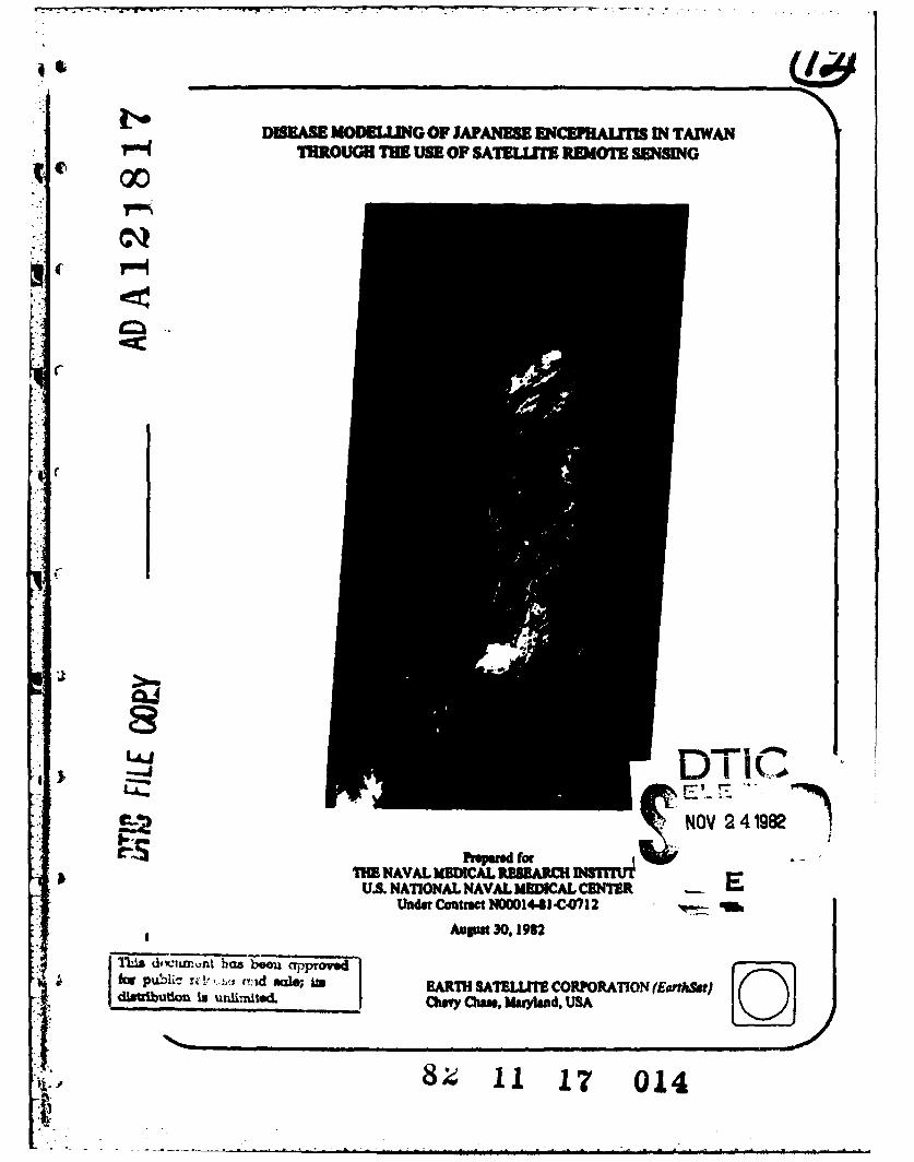
A. The Landsat data base

Landsat coverage of all of Taiwan except the extreme northern

and southern tips of the island is provided by a pair of Landsat frames.

To create the necessary Landsat data base, frames 1101-01550 and 1101-

01552, imaged by the satellite on November 1, 1972, were combined in the

computer to yield a single continuous image (see Report Cover) which contains

a total of approximately 12,000,000 picture elements. The imaged area is

almost cloud-free except in the central mountainous region. There Is,

however, a light fog or haze along most of the western coastal plain,

including much of the land area where disease sites are located. The fog

is most visible in the shortest wavelength band, and shows progressively

less visible in the longer wavelength bands.

The fog may lead to two possible and opposite effects on image classi-

fication:

1. Classification resolution may decrease because image

resolution is decreased; or

2. Fog density may correlate well with general humidity,

which is a potentially significant variable for incidence of

disease; the presence of haze may therefore improve the disease/

Landsat correlations.

Before using Landsat data in the disease distribution models, two

types of radiometric corrections were applied. The first of these, termed

scan line suppression, corrects for the miscalibration of different on-

board detectors in the Multi-Spectral Scanner. An uncorrected image shows

-25-

a characteristic six-line banding pattern, which will degrade the

statistics of the models. In addition to the overall detector miscall-

bratlon, the Taiwan images also contained occasional partial lines of

missing data. In such cases, data values were provided by linear inter-

polation from the nearest neighbor lines of picture elements. This

correction provided images improved in appearance and probably made

little difference to the computed model results since in all cases

examined by eye the dropped data lines were seen only in offshore areas.

The disease incidences were provided as point data, i.e., each was

given at a single latitude and longitude. It is unrealistic to treat them

as point data in the model for several reasons. First, the disease site

data represent disease statistics collected for some defined region (a

village or township) on the ground. Second, in converting latitudes and

longitudes to coordinates on the image, there is a probable error of at

least a few tens of metres, and often a hundred metres or more, in relating

the two different coordinate systems. Third, whatever the geographic

variables may be that control the incidence and spread of the disease, they

are probably spread over several hundred metres on the ground, since the

vector Is mobile over such a range. Fourth, the accuracy of the original

disease site locations is unknown. It is therefore logical to associate

some group of picture elements with each disease site, of a size to be deter-

mined by experiments with the model.

The fourth point above was confirmed when the given disease site

locations were plotted on the Landsat images and on 1:50,000 scale topographic

-26-

maps of the island. Every site was found to be very close to, but

rarely coincident with, a visible town or village. It was concluded

that the towns and villages were intended as the disease sites, but

that the latitudes and longitudes provided had been rounded in value.

Adjustments to the given site locations were therefore made, so as to

center them on the corresponding urban area.

At this point, a new consideration appeared. Clearly, disease data

were collected where people are present. Equally clearly, where people

are present there will be signs of habitation visible on the image data

base. Thus,the strongest likely correlation between disease data and image

data would be one that associated disease with visible signs of human

habitation. However, since the objective of the project is the prediction

of disease-prone areas in regions that may lack any current urban patterns,

correlation with present human activities is not useful. It is therefore

necessary to find a technique that correlates disease occurrence with natural

geographic variables, and not simply with the existence of towns and villages.

This point should be explored a little further. It is certainly true

that villages are likely to be foci for disease occurrence, and that the

number of cases per 100,000 will probably be higher there than in rural parts,

since the vector can readily proceed from one host to the next. However, it

is also likely that ground disturbances introduced by human activity, such as

for example the creation of paddies and ponds, will also serve to increase

the probability of disease occurrence. It is desirable to be able to dissoci-

ate these two factors. The logic used to perform that dissociation is based

upon the fact that the ground disturbances produced by human agricultural

-27-

activity extend well beyond the main towns and villages. If

areas of the Landsat data base are selected that are centered on the

visible urban disease site locations but that exclude the urban develop-

ment itself, correlation of the disease with such areas will reflect

dependence on geography, but not on the visible urban development.

To create the data base needed for the model, sets of "windows"

were therefore selected from the Landsat data. Each window consisted of

a square array of picture elements, with central picture element at a given

disease site. Two different types of windows were used in the models. The

first was a full array, usually lOxlO, which therefore included the central

urban development visible on the image; the second was an array of size

14x14, with the central 10x1O array of picture elements, and hence the

associated urban area, excluded. Model runs were performed using both "full"

and "hollow" windows. The hollow window occupies almost the same ground area

(96 picture elements, or 107 acres) as the full window (100 picture elements,

or 111 acres). See Figure 4.

B. Weather data

Previous work on the etiology of Japanese encephalitis suggests

that in addition to possible correlation with geographic variables there may

be a relationship with climatic variables. Local rainfall, temperature,

and humidity may all be factors in the occurrence and spread of JE.

With this in mind, weather station locations were obtained for Taiwan,

and their positions noted in relation to the disease sites. Only thirteen

stations are present in the island (see Table 1) and it is clear that they

FIGURE 4. Landsat picture element arraysassociated with disease sites.

- -- - - - -- - Full Array, lOxlO

pisLas! sitelo ation

I- -A -

Hollow Array, 1414with excluded lOxlO.4...,.center

Disease si+te location

IIA - - -

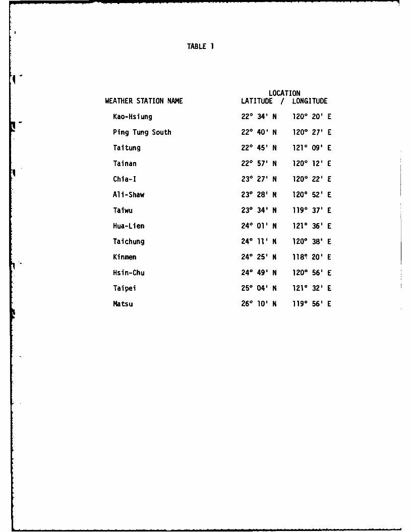
TABLE 1

LOCATIONWEATHER STATION NAME LATITUDE / LONGITUDE

Kao-Hsiung 220 34' N 1200 20' E

Ping Tung South 220 40' N 1200 27' E

Taltung 220 45' N 1210 09' E

Tainan 220 57' N 1200 12' E

Chia-I 230 27' N 1200 22' E

Ali-Shaw 230 28' N 1200 52' E

Taiwu 230 34' N 1190 37' E

Hua-Lien 240 01' N 1210 36' E

Tai chung 240 11' N 1200 38' E

Kinmen 240 25' N 1180 20' E

Hsin-Chu 240 49' N 1200 56' E

Taipei 250 04' N 1210 32' E

Matsu 260 10' N 1190 56' E

-28-

are much too few in number and widely separated in location to contribute

to the highly localized variations in disease occurrence. Weather data

could not therefore contribute significantly to the model, and were

omitted from the analysis. It is still likely that local weather data,

if available, would significantly improve the disease distribution model.

C. Altitude data and location data

The height above sea level of each disease site is available

from 1:50,000 scale topographic maps of the island. Although most population

centers and disease sites lie in the western coastal plain and have altitudes

below 100 metres, the eastern sites lie on higher ground, up to 400 metres.

Altitude is a potentially important variable since it correlates

directly and strongly with temperature and more weakly with humidity and

wind speed, all of which can affect the abundance and distribution of the

vector. The height above sea level was therefore determined from the topo-

graphic maps and included as an additional independent variable. However, since

the altitudes show a strong east-west variation, it is possible that any

observed correlation of disease with altitude indicates dependence not truly

on altitude but on some other variable that also shows east-west differences,

such as the on-shore or off-shore direc.ion of prevailing winds. To test

that hypothesis, a dichotomous variable with values 0 and 1 for eastern and

western site locations was introduced as an alternative to height above sea

level. Both these models were run and results compared.

D. Determination of the set of independent variables

Independent variables such as altitude or location are entered

into the models directly, as continuous or discrete values. In the case of

-29-

the Landsat data, however, this is not possible. The set of 100 picture

elements that comprises a window at one disease site provides 400 reflec-

tance values (values in four spectral bands for every picture element).

An attempt to use these values as independent variables would certainly

fail, since reflectances are highly correlated with each other. There

would in addition be more model coefficients than observations, which also

guarantees a singular set of regression equations. It is therefore

necessary to derive from the 400 reflectances at a disease site some smaller

set of aggregate values to use as independent variables.

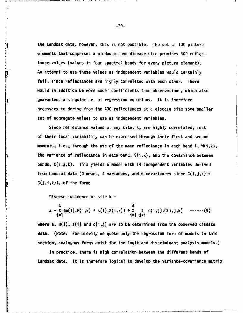
Since reflectance values at any site, k, are highly correlated, most

of their local variability can be expressed through their first and second

moments, i.e., through the use of the mean reflectance in each band i, M(i,k),

the variance of reflectance in each band, S(i,k), and the covariance between

bands, C(i,j,k). This yields a model with 14 independent variables derived

from Landsat data (4 means, 4 variances, and 6 covariances since C(i,j,k) =

C(j,l,k)), of the form:

Disease incidence at site k =

4 4a + E {m(i).M(i,k) + s(l).S(i,k)} + E E c(ij).C(i,j,k) ------ (9)

i=l i=l j<i

where a, m(l), s(i) and c(l,j) are to be determined from the observed disease

data. (Note: For brevity we quote only the regression form of models in this

section; analogous forms exist for the logit and discriminant analysis models.)

In practice, there is high correlation between the different bands of

Landsat data. It is therefore logical to develop the variance-covariance matrix

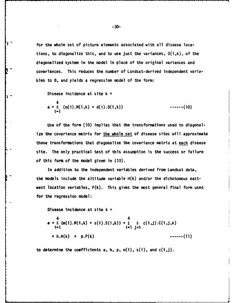
-30-

for the whole set of picture elements associated with all disease loca-

tions, to diagonalize this, and to use just the variances, D(i,k), of the

diagonalized system in the model in place of the original variances and

covarlances. This reduces the number of Landsat-derived independent varia-

bles to 8, and yields a regression model of the form:

Disease incidence at site k =

4a + E (m(i).M(i,k) + d(i).D(i,k)) ------ (10)

1=1

Use of the form (10) implies that the transformations used to diagonal-

ize the covariance matrix for the whole set of disease sites will approximate

those transformations that diagonalize the covariance matrix at each disease

site. The only practical test of this assumption is the success or failure

of this form of the model given in (10).

In addition to the independent variables derived from Landsat data,

the models include the altitude variable H(k) and/or the dichotomous east-

west location variables, P(k). This gives the most general final form used

for the regression model:

Disease incidence at site k =

4 4a + z {m(1).M(i,k) + s(l).S(l,k)) + E E c(i,j).C(i,j,k)

i=1 i-I j<i

+ h.H(k) + p.P(k) ----- (11)

to determine the coefficients a, h, p, m(i), s(i), and c(1,j).

-31-

VI. RESULTS OF THE STATISTICAL MODELS

A. General comparison of the logit and regression models

The first model comparisons were made on a set of 44 disease

sites in south Taiwan, using filled square windows containing 100 picture

elements in each. Computer runs were performed for the linear regression

models and the logit models, first with the means and unrotated variances

of equation (9), then with the means, unrotated variances and covariances

of equation (9), and finally with the means and rotated variances of

equation (10). Since the filled windows include urban areas on the image,

correlations will be expected between density of urban development and

disease occurrences. The first group of tests was therefore regarded as

providing information concerning the preferred models and the number and

type of parameters that should be used in each model, rather than offering

final "best sets" of coefficients for any model.

The first conclusion was that the logit model, while displaying a

goodness-of-fit result that suggests the model is statistically valid, was

not suitable to the problem, largely because the disease occurrence ratios

are so small (from 0 to 0.001). As observed in Section IV.A, the logit

models are designed to handle cases in which the dependent variable takes

on the full range from 0 to 1.

In an attempt to remedy the situation, disease incidence rates per

100,000 were scaled by empirically chosen factors ranging from 10 to 400.

The results of two model runs in which the means and unrotated variances

of the Landsat data were used as independent variables are shown in Tables

2 and 3. Even with the best choice of scaling factor, the results using

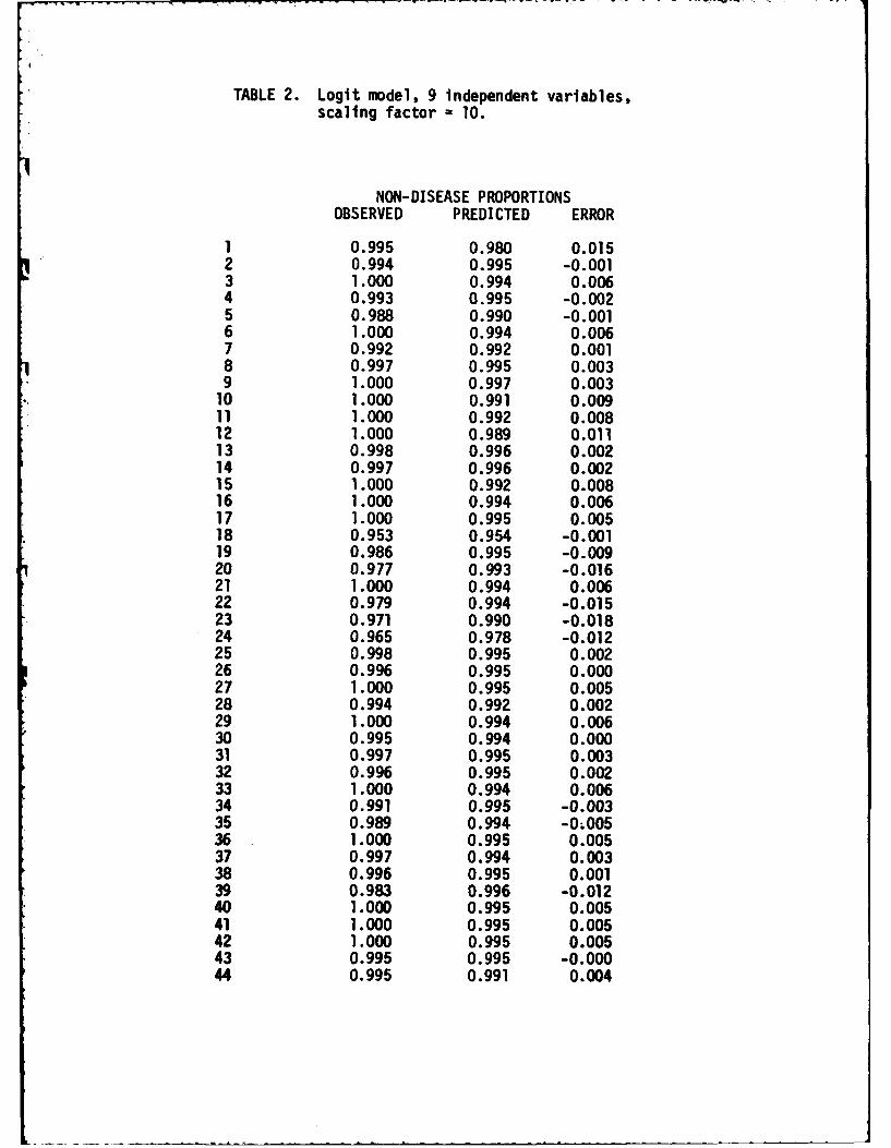
TABLE 2. Loglt model, 9 independent variables,scaling factor = 10.

NON-DISEASE PROPORTIONSOBSERVED PREDICTED ERROR

1 0.995 0.980 0.0152 0.994 0.995 -0.0013 1.000 0.994 0.0064 0.993 0.995 -0.0025 0.988 0.990 -0.0016 1.000 0.994 0.0067 0.992 0.992 0.0018 0.997 0.995 0.0039 1.000 0.997 0.00310 1.000 0.991 0.00911 1.000 0.992 0.00812 1.000 0.989 0.01113 0.998 0.996 0.00214 0.997 0.996 0.00215 1.000 0.992 0.00816 1.000 0.994 0.00617 1.000 0.995 0.00518 0.953 0.954 -0.00119 0.986 0.995 -0.00920 0.977 0.993 -0.01621 1.000 0.994 0.00622 0.979 0.994 -0.01523 0.971 0.990 -0.01824 0.965 0.978 -0.01225 0.998 0.995 0.00226 0.996 0.995 0.00027 1.000 0.995 0.00528 0.994 0.992 0.00229 1.000 0.994 0.00630 0.995 0.994 0.00031 0.997 0.995 0.00332 0.996 0.995 0.00233 1.000 0.994 0.00634 0.991 0.995 -0.00335 0.989 0.994 -0;00536 1.000 0.995 0.00537 0.997 0.994 0.00338 0.996 0.995 0.00139 0.983 0.996 -0.01240 1.000 0.995 0.00541 1.000 0.995 0.00542 1.000 0.995 0.00543 0.995 0.995 -0.00044 0.995 0.991 0.004

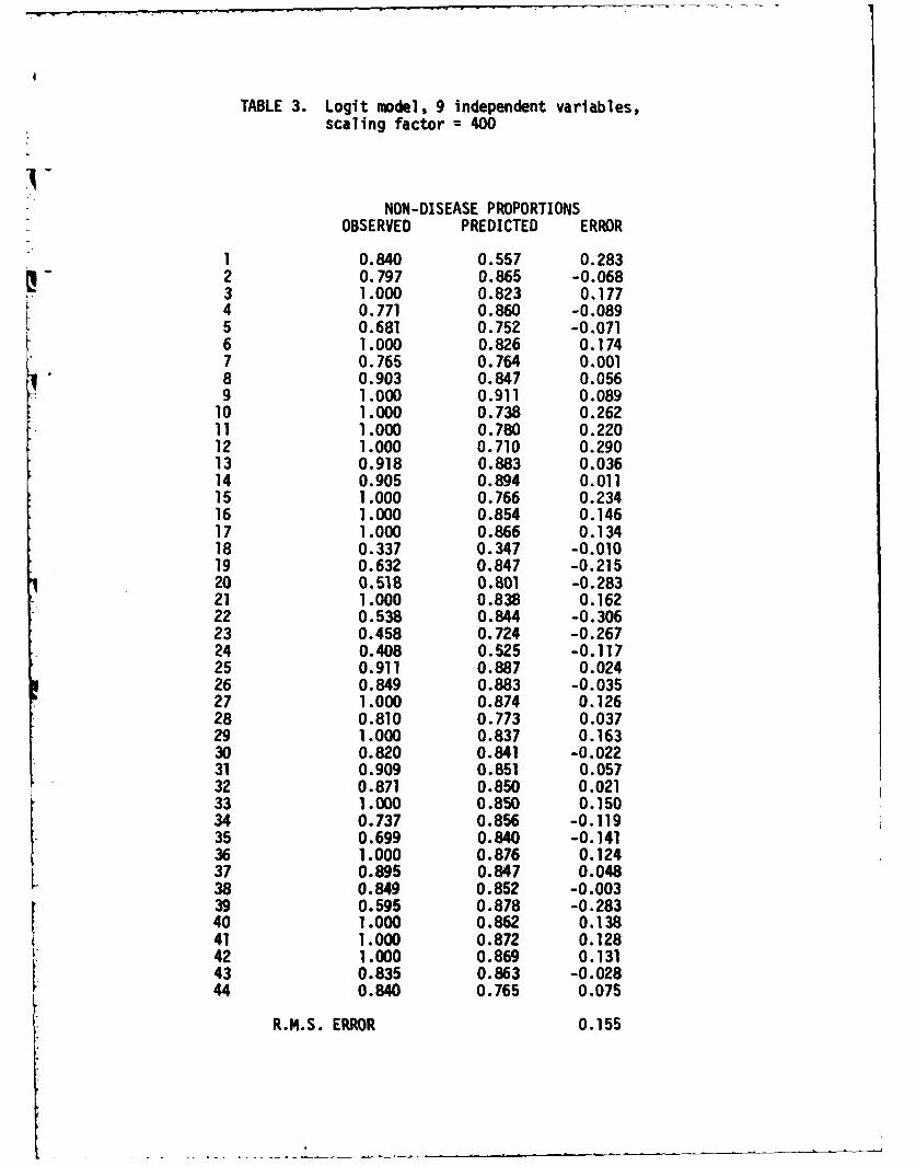
TABLE 3. Logit model, 9 independent variables,scaling factor = 400

NON-DISEASE PROPORTIONSOBSERVED PREDICTED ERROR

1 0.840 0.557 0.2832 0.797 0.865 -0.0683 1.000 0.823 0.1774 0.771 0.860 -0.0895 0.681 0.752 -0.0716 1.000 0.826 0.1747 0.765 0.764 0.0018 0.903 0.847 0.0569 1.000 0.911 0.08910 1.000 0.738 0.26211 1.000 0.780 0.22012 1.000 0.710 0.29013 0.918 0.883 0.03614 0.905 0.894 0.01115 1.000 0.766 0.23416 1.000 0.854 0.14617 1.000 0.866 0.13418 0.337 0.347 -0.01019 0.632 0.847 -0.21520 0.518 0.801 -0.28321 1.000 0.838 0.16222 0.538 0.844 -0.30623 0.458 0.724 -0.26724 0.408 0.525 -0.11725 0.911 0.887 0.02426 0.849 0.883 -0.03527 1.000 0.874 0.12628 0.810 0.773 0.03729 1.000 0.837 0.16330 0.820 0.841 -0.02231 0.909 0.851 0.05732 0.871 0.850 0.02133 1.000 0.850 0.15034 0.737 0.856 -0.11935 0.699 0.840 -0.14136 1.000 0.876 0.12437 0.895 0.847 0.04838 0.849 0.852 -0.00339 0.595 0.878 -0.28340 1.000 0.862 0.13841 1.000 0.872 0.12842 1.000 0.869 0.13143 0.835 0.863 -0.02844 0.840 0.765 0.075

R.M.S. ERROR 0.155

-32-

the logit models were still observed to be generally inferior to those

of the regression models. In later experiments, attention was therefore

focussed on the latter.

A second conclusion, borne out in both the logit and regression

model runs, is that the inclusion of Landsat data covariances decreased

the statistical strength of the results. This indicates that the cross-

correlation terms allow the models to account for an increased amount of

total observational variance, but only at the expense of overfitting the

data. The most successful results were actually obtained using the means

and the unrotated variances of the Landsat data. In later model runs,

attention was therefore focussed on the use of means and unrotated variances

only, plus non-Landsat variables as described below.

B. General results of the discriminant analysis

Using a maximum likelihood classifier and a total of 44 data

points, 22 windows were randomly selected as training sites for the

discriminant analysis, and the remaining 22 sites were reserved as model

test sites. The disease incidence rates were divided into ten ranges,

from zero disease rate to maximum observed disease rate, and each of the

22 windows of the training sites was assigned to the appropriate disease

range based upon the given disease incidence rate. The ten disease ranges

were then regarded as defining ten classes, to which any disease site could

be assigned, and a maximum likelihood classifier was run to determine the

statistical characteristics of the ten classes.

-33-

Each of the 22 test sites was then assigned using the classifier.

The assigned class was then compared with the observed class based on the

actual disease rate.

The results obtained were as follows (this is the average obtained

from six different runs and assignments of class range):

Test sites classified correctly: 3

Test sites classified with error of one range: 5

Test sites classified with error of two ranges: 2

Test sites classified with error of three ranges: 4

Test sites classified with error of four ranges: 1

Test sites classified with error of five ranges: 2

Test sites classified with error of six ranges: 3

Test sites classified with error of seven ranges: 0

Test sites classified with error of eight ranges: 2 TOTAL: 22 sites

On a purely random basis, if there were no correlation at all between

training site and test site ranges, the average error in test site ranges

would be 3.3 units. The observed error in test site ranges had an average

of 3.14. This is consistent with a random classification result. The

discriminant analysis model was therefore judged unsatisfactory for this

application. A second series of tests, employing 63 disease sites, gave

similar results.

To summarize these findings, the discriminant analysis techniques proved

unable to define "clean" classes of Landsat data that corresponded to disease

incidence. Classes contained widely scattered data points, and assignment of

-34-

a data point to a particular class was ambiguous. This is probably due

to the degree of variability of Landsat data, considered on an individual

picture element-by-picture element basis. The averaging over many Landsat

picture elements employed in the logit and regression models thus appear

central to the development of a successful model.

C. Results of the regression models and the addition of other

variables

All the computer runs described in VI.A and B used Landsat variables

alone as independent variables. Based on those results, it was decided to

focus on regression models for subsequent experiments with the data.

1. Results comparing different independent variables drawnfrom Landsat data

Initial runs of the regression model, as already noted,

employed data from 44 disease sites in southern Taiwan, and a filled

lOxlO array of Landsat picture elements centered at disease sites.

Runs were performed using means and unrotated variances only; means,

variances and covariances; and means and rotated variances.

The results were as follows:

a. Means and unrotated variances: R2 = 0.42

b. Means, variances and covarlances: R2 = 0.35

c. Means and rotated variances: R2 = 0.38

This indicates that inclusion of the covariances over-fits the data,

and that use of the rotated variances for the whole data set degrades

the results, presumably because the rotations that are suitable for

the whole set of picture element arrays are not suitable for the arrays

considered separately.

-35-

2. Results using filled versus hollow arrays

It had been observed in early runs of the regression

model that worse fits were obtained if the array centers did not

quite correspond to the disease site location. It was this

observation that led to a suspicion that the main correlations

obtained were with visible urban development, rather than natural

geographic variables. This led in turn to the use of hollow

arrays of picture elements that would exclude the central urban

area associated with a disease site.

Using the regression model with a l0xlO full window and then

a 14x14 hollow window, the results were as follows (the data base

was again a set of 44 disease sites in southern Taiwan):

a. Filled window: R2 = 0.42

b. Hollow window: R2 = 0.37

Using a set of 57 disease sites, in northern and southern

Taiwan, the corresponding results were:

a. Filled windows: R2 = 0.42

b. Hollow windows: R2 = 0.39

The exact equality of R2 (to 2 significant figures) for the filled

window results is no more than coincidental, since the individual

residuals at particular disease sites show no particular pattern.

However, the higher value of R2 obtained with filled windows con-

firmed the conjecture that the correlation was partly with urban

features, rather than with natural geographic variables. With the

hollow windows, there is weak positive correlation (the correlation

coefficient ranged from 0.61 to 0.65 in different model runs). In

-36-

view of the fact that it is correlations with natural geography

that are sought, rather than relation of disease to urban develop-

ments, hollow windows were used throughout the remaining model

runs, despite the rather lower correlations that this produced in

the above tests.

3. Results including other variables

Using data from 44 disease sites in southern Taiwan,

and hollow 14xl4 arrays at each site, altitude was now added as

an independent variable. In a second series of runs on the same

data, east/west location was added as a dichotomous variable.

Finally, runs were performed using altitude alone, in order to

explore the extent to which this might account for all significant

correlation with disease incidence.

The results obtained are as follows:

- a. Landsat data alone: R2 = 0.37

b. Landsat data plus altitude: R2 = 0.57

c. Landsat data plus east/west position: R2 = 0.40

- d. Altitude data alone: R2 = 0.41

The individual residuals showed no particular pattern.

D. Other experiments and the summary of results

A complete testing of all models would require computer runs

with all available data sets, with filled and hollow windows, with rotated

and unrotated variances, and with altitude and east/west location included

and excluded. Consideration of all such combinations would lead to an

-37-

impossibly high number of computer runs. The sequential method described

in the previous three sections was therefore employed, in which only the

best model at each stage was used in subsequent experiments.

This procedure can be criticized as too restrictive, since there is

always the possibility that a model rejected early on the basis of a set

of experiments would prove superior when other variations were later per-

formed. To provide a limited test of this, additional model runs were

performed using the 44 site data set, altitude data, and hollow array windows.

As a separate check on the discriminant analysis approach, the logit classi-

fier was used as a non-parametric maximum-likelihood classifier.

The results of these runs supported those of Section VI.C, i.e., the

regression model gave better results than either the logit model or the

discriminant analysis, and altitude information plus Landsat data gave stronger

correlations than any other combination of variables. The runs with filled

arrays continued to give higher correlation than those with hollow arrays, but

the suspicion that this is due mainly to correlation with urban land use

remains.

The overall results of all experiments can therefore be summarized as

follows:

1. Of the types of models employed on the project, regression

models proved superior to either logit models or discriminant models.

2. A regression model with g independent variables provided

the best correlations with the disease data.

3. Hollow arrays of Landsat data surrounding each disease

incidence site were judged necessary, to eliminate the effects of

urban development on computed correlations.

i -

-38-

4. The best combination of variables consists of

Landsat-derived variables (means and variances) plus altitude.

5. Using the best model, a value of R2 = 0.57 (corre-

lation coefficient = 0.75) was obtained. This is statistically

significant.

6. Varying the input data to include different numbers

and locations of disease test sites produced only small effects

on the computed results (R2 ranged from 0.51 with only 15 sites,

to 0.56 with 63 sites). The model thus appears insensitive to

the particular choice of sites, either in number or placement.

7. No systematic bias could be observed in computed

results, and the residuals at disease sites appear to be uncorre-

lated with location, altitude, or degree of urban development.

Possible correlation of residuals with temperature, humidity, and

precipitation is still unknown.

-39-

- VII. CONCLUSIONS

The objective of this study was to explore statistical relationships

between geographic variables, principally those obtained by the Landsat

1 - satellite systems, and the observed occurrence of Japanese encephalitis on

Taiwan. To accomplish this end, Landsat data, location data (latitude and

longitude) and altitude data were employed to develop four different types

of statistical model, namely, linear regressions, log-linear regressions,

logit models, and discriminant analyses. Observed disease incidence for the

period 1968-1975, for 106 sites in Taiwan, constituted the dependent variable.

Landsat data were used in the form of the means, variances and co-

variances associated with surface reflectance for groups of picture elements

centered on disease incidence locations. Both unrotated and rotated

(principal component) variances were employed in the models.

Following a substantial series of experimental computer runs, it was

concluded that the linear regression models give the best results of the four

models considered. In particular, the preferred model is a 9-variable linear

regression, employing as independent variables Landsat means and unrotated

variances (drawn from 96-pixel hollow windows surrounding each disease inci-

dence site), together with altitudes. With this model a statistically

significant correlation (correlation coefficient 0.75) is obtained between

the observed and predicted disease incidences.

Computer runs performed using different data sets suggest that the

results are insensitive to the number and position of disease sites used to

determine the model coefficients. In addition, the residuals (the difference

of observed and computed values) display no systematic bias in terms of

t2-40-

location, altitude, or other geographic variable. The technique there-

fore shows promise as a predictive tool for geographic areas where disease

data are lacking, or of doubtful quality.

- Although the results described are specific to the single disease

of Japanese encephalitis in a particular location, the methods used

and programs developed are quite general. The form of model and data

manipulations should be applicable to infectious diseases with airborne

insect vectors, in any location.

The study was conducted under a number of significant constraints, and

stronger results may be obtained if one or more of them could be relaxed.

The most important constraint is probably the fact that the Landsat data

base was drawn from a single date (November 1, 1972). The information revealed

by Landsat certainly changes significantly with season, and has substantial

year-by-year variations. Additional constraints were provided by the absence

of suitably detailed weather data, by the uncertain quality of the disease

incidence data, and by a practical limitation on the number ef different window

sizes and statistical techniques that could be employed.

Given these restrictions, the positive correlations observed between

disease incidence and Landsat observables is encouraging, and perhaps even

surprising. It would be natural for disease occurrence to correlate with

urbanization, but since urban centers were excluded by the use of hollow windows,

the correlation is almost certainly due to a real relationship between geo-

graphic variables (which may nclude human agricultural practices) and distase

occurrence.

-41-

The distribution model developed here is no more than a beginning.

Additional effort is needed to confirm present results using satellite data

of different dates; to extend the model geographically, ideally to other

countries and to different topographic and climatic environments; and to

explore through biological and geographic analysis the reasons for Landsat's

positive correlation with observed disease. Beyond this, it is natural to

consider application to other diseases, with other airborne or waterborne

vectors.

In all cases, the satellite data base is already available, and use of

weather satellites in addition to Landsat may pemit the inclusion of climatic

variables to supplement ground weather station information. The limiting

factor on future investigations will probably be the availability of suitable

disease data.

REFERENCES

1 - 1. G. Fracastoro, "De Contagionibus et Contagiosis Morbis et EorumCuratione" (On Contagion, Contagious Diseases, and Their Cure);1546, tr. W. C. Wright, Putnam's, 1930.

2. L. Pasteur "Etudes sur les maladies des vers a soie" (1870).

3. R. Koch "Die Aetiologie der Tuberculose" (The Aetiology ofTuberculosis); 1882, tr. M. Pinner, Am. Rev. Tuber., March,1932.

4. Theobald Smith & F. L. Kilborne, "Investigations into the Nature,Causation and Prevention of Southern Cattle Fever"; Bureau ofAnimal Industry, 1893.

5. Walter Reed, "The Propagation of Yellow Fever; Observations Basedon Recent Researches" Med. Rec. 60, No. 6, August 1901.

6. W. A. Fischer et al., "History of Remote Sensing"; in Manual ofRemote Sensing, ed. R. G. Reeves, pp. 27-29; American Society ofPhotogrammetry, Falls Church, Virginia (1975).

7. Ibid., pp. 31-34.

8. Ibid., pp. 35-36 and 40-41.

9. Principal Investigators, Earth Resources Technology Satellite-A.Goddard Space Flight Center report (undated; the PrincipalInvestigator agreements listed were those signed as of June 21, 1972).

10. G. Arp et al., "System Development of the Screwworm Eradication DataSystem"; Johnson Space Center Technical Memorandum JSC-10965 (1976).

11. C. Sheffield, "Earth Resources and Satellite Imaging Systems";Interdisciplinary Science Reviews, Volume 7, Number 2, Heyden,London (1982).

12. J. T. Grayston, San-Pin Wang, and Chun-hui Yen, "Encephalitis onTaiwan, I: Introduction and Epidemiology"; American Journal ofTropical Medicine and Hygiene, Vol. II, No. 1, pp. 126-161 (1962).

13. T. S. Hsu, C. T. Huang, and S. T. Hsu, "Epidemiology and Control ofJapanese Encephalitis in Taiwan"; Japan Journal of Tropical Medicine,Vol. 10, pp. 165-174 (1969).

14. S. M. Wang, "Japanese Encephalitis on Taiwan"; United States MedicalResearch Unit, Lecture and Review Series, Report No. 62-4 (1962).

15. H. S. Hurlbut, "The Ecology of Japanese Encephalitis Virus"; UnitedStates Medical Research Unit, Lecture and Review Series, Report No.63-2 (1983).

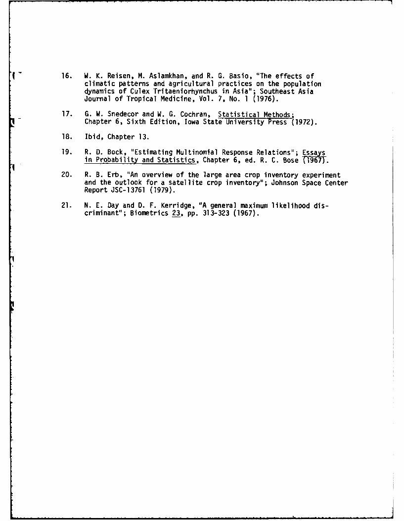
16. W. K. Reisen, M. Aslamkhan, and R. G. Basio, "The effects ofclimatic patterns and agricultural practices on the populationdynamics of Culex Tritaeniorhynchus in Asia"; Southeast AsiaJournal of Tropical Medicine, Vol. 7, No. 1 (1976).

17. G. W. Snedecor and W. G. Cochran, Statistical Methods;Chapter 6, Sixth Edition, Iowa State University Press (1972).

18. Ibid, Chapter 13.

19. R. D. Bock, "Estimating Multinomlal Response Relations"; Essaysin Probability and Statistics, Chapter 6, ed. R. C. Bose1

20. R. B. Erb, "An overview of the large area crop inventory experimentand the outlook for a satellite crop inventory"; Johnson Space CenterReport JSC-13761 (1979).

21. N. E. Day and D. F. Kerridge, "A general maximum likelihood dis-criminant"; Biometrics 23, pp. 313-323 (1967).

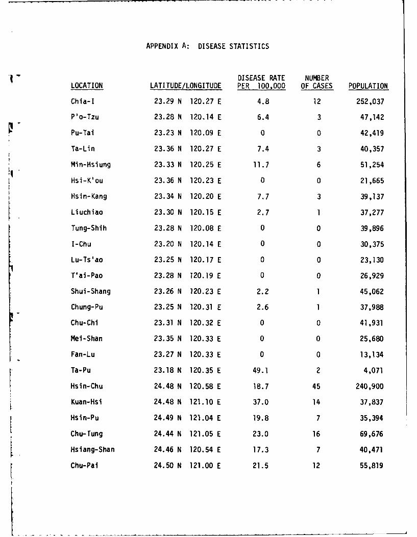
APPENDIX A: DISEASE STATISTICS

DISEASE RATE NUMBERLOCATION LATITUDE/LONGITUDE PER 100,000 OF CASES POPULATION

Chia-I 23.29 N 120.27 E 4.8 12 252,037

P'o-Tzu 23.28 N 120.14 E 6.4 3 47,142

Pu-Tai 23.23 N 120.09 E 0 0 42,419

Ta-Lin 23.36 N 120.27 E 7.4 3 40,357

Min-Hsiung 23.33 N 120.25 E 11.7 6 51,254

Hsi-K'ou 23.36 N 120.23 E 0 0 21,665

Hsin-Kang 23.34 N 120.20 E 7.7 3 39,137

Liuchiao 23.30 N 120.15 E 2.7 1 37,277

Tung-Shih 23.28 N 120.08 E 0 0 39,896

I-Chu 23.20 N 120.14 E 0 0 30,375

Lu-Ts'ao 23.25 N 120.17 E 0 0 23,130

T'ai-Pao 23.28 N 120.19 E 0 0 26,929

Shui-Shang 23.26 N 120.23 E 2.2 1 45,062

Chung-Pu 23.25 N 120.31 E 2.6 1 37,988

Chu-Chi 23.31 N 120.32 E 0 0 41,931

Mei-Shan 23.35 N 120.33 E 0 0 25,680

Fan-Lu 23.27 N 120.33 E 0 0 13,134

Ta-Pu 23.18 N 120.35 E 49.1 2 4,071

Hsin-Chu 24.48 N 120.58 E 18.7 45 240,900

Kuan-Hsi 24.48 N 121.10 E 37.0 14 37,837

Hsin-Pu 24.49 N 121.04 E 19.8 7 35,394

Chu-Tung 24.44 N 121.05 E 23.0 16 69,676

Hslang-Shan 24.46 N 120.54 E 17.3 7 40,471

Chu-Pai 24.50 N 121.00 E 21.5 12 55,819

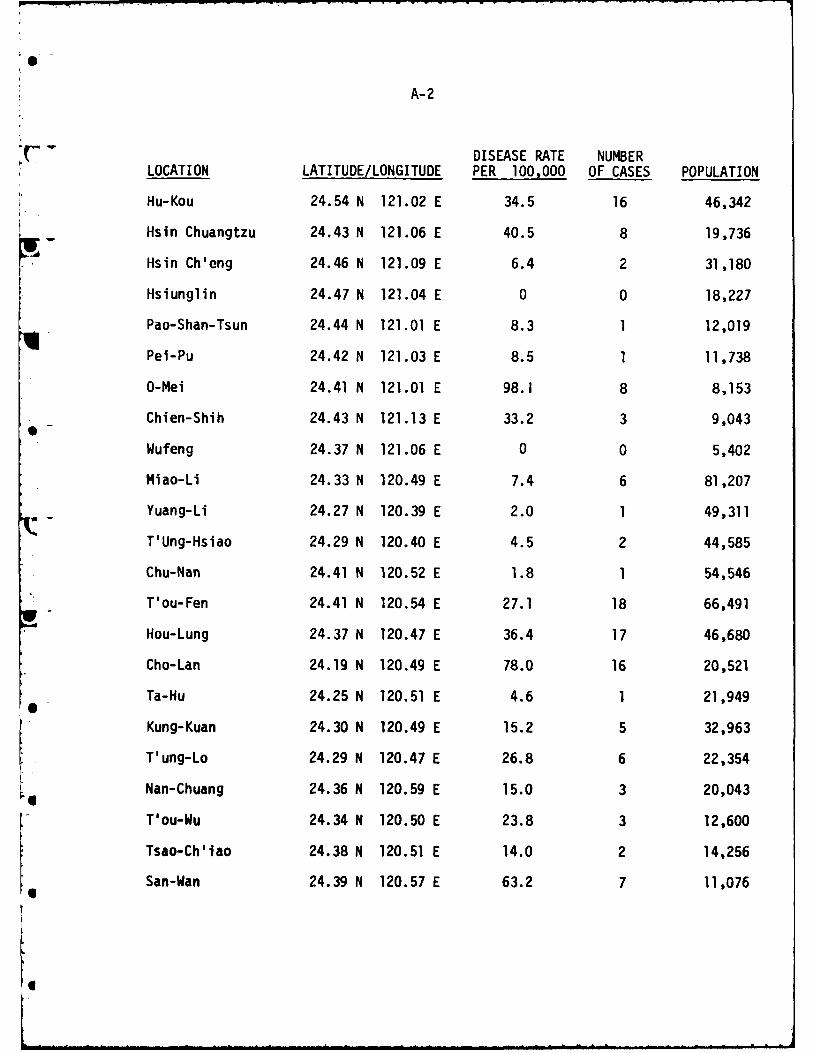
A-2

DISEASE RATE NUMBERLOCATION LATITUDE/LONGITUDE PER 100,000 OF CASES POPULATION

Hu-Kou 24.54 N 121.02 E 34.5 16 46,342

Hsin Chuangtzu 24.43 N 121.06 E 40.5 8 19,736

Hsin Ch'eng 24.46 N 121.09 E 6.4 2 31,180

Hsiunglin 24.47 N 121.04 E 0 0 18,227

Pao-Shan-Tsun 24.44 N 121.01 E 8.3 1 12,019

Pei-Pu 24.42 N 121.03 E 8.5 1 11,738

O-Mei 24.41 N 121.01 E 98.1 8 8,153

Chien-Shih 24.43 N 121.13 E 33.2 3 9,043

Wufeng 24.37 N 121.06 E 0 0 5,402

Miao-Li 24.33 N 120.49 E 7.4 6 81,207

Yuang-Li 24.27 N 120.39 E 2.0 1 49,311

T'Ung-Hsiao 24.29 N 120.40 E 4.5 2 44,585

Chu-Nan 24.41 N 120.52 E 1.8 1 54,546

T'ou-Fen 24.41 N 120.54 E 27.1 18 66,491

Hou-Lung 24.37 N 120.47 E 36.4 17 46,680

Cho-Lan 24.19 N 120.49 E 78.0 16 20,521

Ta-Hu 24.25 N 120.51 E 4.6 1 21,949l

Kung-Kuan 24.30 N 120.49 E 15.2 5 32,963

T'ung-Lo 24.29 N 120.47 E 26.8 6 22,354

Nan-Chuang 24.36 N 120.59 E 15.0 3 20,043

T'ou-Wu 24.34 N 120.50 E 23.8 3 12,600

Tsao-Ch'lao 24.38 N 120.51 E 14.0 2 14,256

San-Wan 24.39 N 120.57 E 63.2 7 11,076Ul

A-3

DISEASE RATE NUMBERLOCATION LATITUDE/LONGITUDE PER 100,000 OF CASES POPULATION

Shih-T'an 24.32 N 120.55 E 34.4 3 8,710

Hua-Lien 23.58 N 121.36 E 7.8 8 102,665

Feng-Lin 23.43 N 121.26 E 15.1 3 19,857

Yu-Li 23.20 N 121.18 E 14.6 6 41,225

Hsin-Ch'eng 24.08 N 121.39 E 11.4 2 17,510

Chi-An 23.58 N 121.33 E 30.8 15 48,771

Shou-Feng 23.52 N 121.30 E 23.6 6 25,398

Kuang-Fu 23.23 N 121.19 E 23.2 5 21,519

Feng-Pien Ts'un 23.36 N 121.31 E 0 0 8,699

Jui-Sui 23.30 N 121.22 E 21.5 4 18,603

Fu-Li Ts'un 23.10 N 121.14 E 29.6 6 20,263

Hsiulin 24.07 N 121.37 E 27.7 4 14,430

Cho-Hsi Ts'un 23.21 N 121.17 E 36.3 3 8,274

Chang-Hua 24.05 N 120.32 E 10.0 18 181,359

Lu-Kang 24.03 N 120.25 E 16.6 12 72,474

Ho-Mei 24.06 N 120.29 E 12.2 8 65,337

Pei-Tou 23.52 N 120.31 E 7.0 2 28,767

Yuan-Lin 23.57 N 120.34 E 4.9 5 102,554

Hsi-Hu 23.57 N 120.28 E 4.3 2 46,259

T'len-Chung 23.52 N 120.35 E 0 0 45,374

Erh-Lin 23.54 N 120.21 E 1.7 1 59,579

Hslenhsl 24.08 N 120.27 E 0 0 15,000

Shen-Kang 24.09 N 120.28 E 18.8 5 26.649

Fushing 24.03 N 120.24 E 15.0 6 10,214

A-4

K DISEASE RATE NUMBERLOCATION LATITUDE/LONGITUDE PER 100,000 OF CASES POPULATION

Hsiushui 24.03 N 120.30 E 10.0 3 30,010

- Huatan 24.02 N 120.32 E 8.2 3 36,653

Fenyuan 24.01 N 120.37 E 18.2 5 27,467

Tatsun 24.00 N 120.32 E 0 0 31,130

1 - Pu-Yen Ts'un 23.59 N 120.28 E 5.9 2 33,815

P'u-Hsin 23.57 N 120.32 E 0 0 31,144

Yung-Ching 23.55 N 120.32 E 2.7 1 36,615

She-T'ou 23.54 N 120.35 E 0 0 39,828

Erh-Shui 23.49 N 120.36 E 0 0 22,545

Tienwei 23.54 N 120.30 E 0 0 29,130

Pitou 23.54 N 120.28 E 0 0 33,846

Fang-Wan 23.55 N 120.18 E 0 0 45,824

Ta-Ch'eng 23.52 N 120.19 E 3.6 1 27,443

Chu-T'ang 23.52 N 120.25 E 0 0 20,584

Chichou 23.51 N 120.29 E 0 0 36,838

Tun-Lin 23.42 N 120.31 E 2.4 2 81,651

Tou-Nan 23.41 N 120.28 E 4.6 2 44,895

Hu-Wei 23.43 N 120.25 E 0 0 66,570

Hsi-Lo 23.48 N 120.27 E 5.8 3 51,306

Tuku 23.41 N 120.23 E 0 0 35,724

Pei-Kang 23.34 N 120.17 E 5.5 3 54,552

Ku-K'eng 23.39 N 120.33 E 2.5 1 39,758

Tapi 23.39 N 120.25 E 3.7 1 27,020

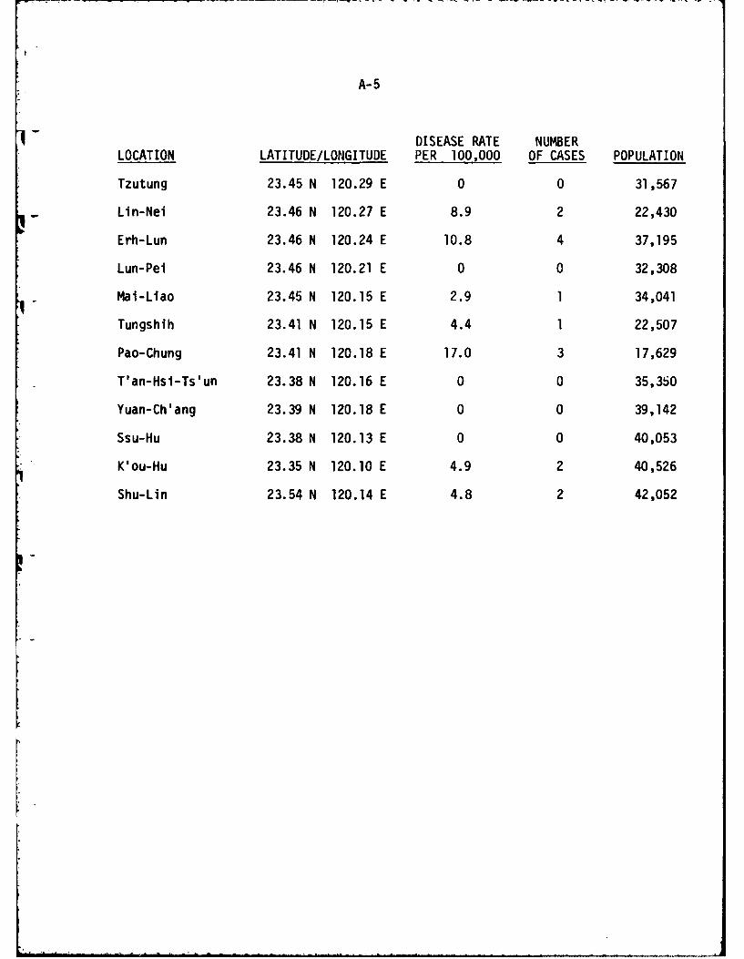
A-5

DISEASE RATE NUMBER

LOCATION LATITUDE/LONGITUDE PER 100,000 OF CASES POPULATION

Tzutung 23.45 N 120.29 E 0 0 31,567

Lin-Nei 23.46 N 120.27 E 8.9 2 22,430

Erh-Lun 23.46 N 120.24 E 10.8 4 37,195

Lun-Pei 23.46 N 120.21 E 0 0 32,308

Mai-Liao 23.45 N 120.15 E 2.9 1 34,041

Tungshih 23.41 N 120.15 E 4.4 1 22,507

Pao-Chung 23.41 N 120.18 E 17.0 3 17,629

T'an-Hsi-Ts'un 23.38 N 120.16 E 0 0 35,350

Yuan-Ch'ang 23.39 N 120.18 E 0 0 39,142

Ssu-Hu 23.38 N 120.13 E 0 0 40,053

K'ou-Hu 23.35 N 120.10 E 4.9 2 40,526

Shu-Lin 23.54 N 120.14 E 4.8 2 42,052

4

OFFICE OF NAVA. Rr:SF:ARCIIIlN CROBI OLOGY PROGIUM

STX\\L)AD DI STRI BLUI'ION LI ST

Nunber of Copies:

( 12 ) Administrator, Defense Technical Informa-tion Center

Cameron StationAlexandria, VA 22314

(6) Director, Naval Research LaboratoryAttn: Technical Information DivisionCode 2627Washington, D.C. 20375

(3) Office of Naval ResearchDepartment of the NavyCode 443800 N. Quincy StreetArlington, VA 22217

(1) Commanding Officer (Code 00)Naval Medical Research & Development CommandNational Naval Medical CenterBethesda, MD 20014

( 1 ) Naval Medical Research & Development CommandCode 46National Naval Medical CenterBethesda, MD 20014

(2) Technical Reference LibraryNaval Medical Research InstituteNational Naval Medical CenterBethesda, MD 20014

(2) Bureau of Medicine and SurgeryNavy DepartmentCode MFD 314Washington, D.C. 20372

(1 ) Office of Naval Research Eastern/CentralRegional Office

Building 114, Section D666 Sumner StreetBoston, MA 02210

STA,%RD DISTIBUTION LIST (Cont'd)

Nuznber of Copies:

(1) Office of Naval Research Branch Office536 South Clark StreetChicago, IL 60605

(1) Office of Naval Research Western RegionalOffice

1030 East Green StreetPasadena, CA 91106

I1) Commanding OfficerU.S. Naval Medical Research Unit #2APO, San Francisco 96528

(1 ) Commanding OfficerU.S. Naval W-dical Research Unit #3FPO, New York 09527

(1) Officer in ChargeSubmarine Medical Research LaboratoryU.S. Naval Submarine Base, New LondonGroton, CT 06342

( 1 ) Scientific LibraryNaval Biosciences LaboratoryNaval Supply CenterOakland, CA 94625

(1 ) Scientific LibraryNaval Aerospace Medical Research InstituteNaval Aerospace Medical CenterPensacola, FL 32512

(1 ) Commander, Naval Air Development CenterAttn: Code 6003Warminster, PA 18974

(1) Conmanding GeneralU.S. Army Medical Research & Development

ComandFort DetrickFrederick, MD 21701Attn: INIEDDH-Sr

S'fAND1ARD DI STRI BUTION LI ST (Cont' d)

Number of Copies:

(1 ) Director of Life SciencesAir Force Office of Scientific ResearchBolling Air Force BaseWashington, D.C. 20032

(1 ) STIC-224301 Suitland RoadWashington, D.C. 20390

(1 ) DirectorWalter Reed Army Institute of ResearchWalter Reed Army Medical CenterWashington, D.C. 20012

FILMED

lm83

DTIC