discovering latent network structure in point … latent network structure in point process ......

DISCOVERING LATENT NETWORK STRUCTURE INPOINT PROCESS DATA

By Scott W. Linderman and Ryan P. Adams

Harvard University

Networks play a central role in modern data analysis, enablingus to reason about systems by studying the relationships betweentheir parts. Most often in network analysis, the edges are given. How-ever, in many systems it is difficult or impossible to measure thenetwork directly. Examples of latent networks include economic in-teractions linking financial instruments and patterns of reciprocity ingang violence. In these cases, we are limited to noisy observations ofevents associated with each node. To enable analysis of these implicitnetworks, we develop a probabilistic model that combines mutually-exciting point processes with random graph models. We show howthe Poisson superposition principle enables an elegant auxiliary vari-able formulation and a fully-Bayesian, parallel inference algorithm.We evaluate this new model empirically on several datasets.

1. Introduction. Many types of modern data are characterized via relationships on a network.Social network analysis is the most commonly considered example, where the properties of individ-uals (vertices) can be inferred from “friendship” type connections (edges). Such analyses are alsocritical to understanding regulatory biological pathways, trade relationships between nations, andpropagation of disease. The tasks associated with such data may be unsupervised (e.g., identifyinglow-dimensional representations of edges or vertices) or supervised (e.g., predicting unobserved linksin the graph). Traditionally, network analysis has focused on explicit network problems in which thegraph itself is considered to be the observed data. That is, the vertices are considered known andthe data are the entries in the associated adjacency matrix. A rich literature has arisen in recentyears for applying statistical machine learning models to this type of problem, e.g., Liben-Nowell& Kleinberg (2007); Hoff (2008); Goldenberg et al. (2010).

In this paper we are concerned with implicit networks that cannot be observed directly, but aboutwhich we wish to perform analysis. In an implicit network, the vertices or edges of the graph maynot be directly observed, but the graph structure may be inferred from noisy emissions. These noisyobservations are assumed to have been generated according to underlying dynamics that respectthe latent network structure.

For example, trades on financial stock markets are executed thousands of times per second.Trades of one stock are likely to cause subsequent activity on stocks in related industries. Howcan we infer such interactions and disentangle them from market-wide fluctuations that occurthroughout the day? Discovering latent structure underlying financial markets not only revealsinterpretable patterns of interaction, but also provides insight into the stability of the market. InSection 4 we will analyze the stability of mutually-excitatory systems, and in Section 6 we willexplore how stock similarity may be inferred from trading activity.

As another example, both the edges and vertices may be latent. In Section 7, we examine patternsof violence in Chicago, which can often be attributed to social structures in the form of gangs. Wewould expect that attacks from one gang onto another might induce cascades of violence, butthe vertices (gang identity of both perpetrator and victim) are unobserved. As with the financialdata, it should be possible to exploit dynamics to infer these social structures. In this case spatial

1

arX

iv:1

402.

0914

v1 [

stat

.ML

] 4

Feb

201

4

2 S. W. LINDERMAN AND R. P. ADAMS

information is available as well, which can help inform latent vertex identities.In both of these examples, the noisy emissions have the form of events in time, or “spikes,” and

our intuition is that a spike at a vertex will induce activity at adjacent vertices. In this paper,we formalize this idea into a probabilistic model based on mutually-interacting point processes.Specifically, we combine the Hawkes process (Hawkes, 1971) with recently developed exchangeablerandom graph priors. This combination allows us to reason about latent networks in terms of theway that they regulate interaction in the Hawkes process. Inference in the resulting model can bedone with Markov chain Monte Carlo, and an elegant data augmentation scheme results in efficientparallelism.

2. Preliminaries.

2.1. Poisson Processes. Point processes are fundamental statistical objects that yield randomfinite sets of events {sn}Nn=1 ⊂ S, where S is a compact subset of RD, for example, space or time.The Poisson process is the canonical example. It is governed by a nonnegative “rate” or “intensity”function, λ(s) : S → R+. The number of events in a subset S ′ ⊂ S follows a Poisson distributionwith mean

∫S′ λ(s)ds. Moreover, the number of events in disjoint subsets are independent.

We use the notation {sn}Nn=1 ∼ PP(λ(s)) to indicate that a set of events {sn}Nn=1 is drawn froma Poisson process with rate λ(s). The likelihood is given by

p({sn}Nn=1|λ(s)) = exp

{−∫Sλ(s)ds

} N∏n=1

λ(sn).(1)

In this work we will make use of a special property of Poisson processes, the Poisson superpositiontheorem, which states that {sn} ∼ PP(λ1(s) + . . .+ λK(s)) can be decomposed intoK independentPoisson processes. Letting zn denote the origin of the n-th event, we perform the decomposition byindependently sampling each zn from Pr(zn = k) ∝ λk(sn), for k ∈ {1 . . .K} (Daley & Vere-Jones,1988).

2.2. Hawkes Processes. Though Poisson processes have many nice properties, they cannot cap-ture interactions between events. For this we turn to a more general model known as Hawkesprocesses. A Hawkes process consists of K point processes and gives rise to sets of marked events{sn, cn}Nn=1, where cn ∈ {1, . . . ,K} specifies the process on which the n-th event occurred. For now,we assume the events are points in time, i.e., sn ∈ [0, T ]. Each of the K processes is a conditionallyPoisson process with a rate λk(t | {sn : sn < t}) that depends on the history of events up to time t.

Hawkes processes have additive interactions. Each process has a “background rate” λ0,k(t), andeach event sn on process k adds a nonnegative impulse response hk,k′(t − sn) to the intensity ofother processes k′. Causality and locality of influence are enforced by requiring hk,k′(∆t) to be zerofor ∆t /∈ [0,∆tmax].

By the superposition theorem for Poisson processes, these additive components can be consideredindependent processes, each giving rise to their own events. We augment our data with a latentrandom variable zn ∈ {0, . . . , n− 1} to indicate the cause of the n-th event (0 if the event is due tothe background rate and 1 . . . n− 1 if it was caused by a preceding event).

Let Cn,k′ denote the set of events on process k′ that were parented by event n. Formally,

Cn,k′ ≡ {sn′ : cn′ = k′ ∧ zn′ = n}.

DISCOVERING LATENT NETWORK STRUCTURE IN POINT PROCESS DATA 3

1

2

3

4

5a

5b

5c

I

II

III

Fig 1: Illustration of a Hawkes process. Events induce impulse responses on connected processesand spawn “child” events. See the main text for a complete description.

Let C0,k be the set of events attributed to the background rate of process k. The augmented Hawkeslikelihood is the product of likelihoods of each Poisson process:

p({(sn, cn, zn)}Nn=1 | {λ0,k(t)},{{hk,k′(∆t)}}) =[K∏k=1

p(C0,k |λ0,k(t))

]×

[N∏n=1

K∏k=1

p(Cn,k |hcn,k(t− sn))

],(2)

where the densities in the product are given by Equation 1.Figure 1 illustrates a causal cascades of events for a simple network of three processes (I-III).

The first event is caused by the background rate (z1 = 0), and it induces impulse responses onprocesses II and III. Event 2 is spawned by the impulse on the third process (z2 = 1), and feedsback onto processes I and II. In some cases a single parent event induces multiple children, e.g.,event 4 spawns events 5a-c. In this simple example, processes excite one another, but do not excitethemselves. Next we will introduce more sophisticated models for such interaction networks.

2.3. Random Graph Models. Graphs of K nodes correspond to K ×K matrices. Unweightedgraphs are binary adjacency matrices A where Ak,k′ = 1 indicates a directed edge from node k tonode k′. Weighted directed graphs can be represented by a real matrixW whose entries indicate theweights of the edges. Random graph models reflect the probability of different network structuresthrough distributions over these matrices.

Recently, many random graph models have been unified under an elegant theoretical frameworkdue to Aldous and Hoover (Aldous, 1981; Hoover, 1979). See Lloyd et al. (2012) for an overview.Conceptually, the Aldous-Hoover representation characterizes the class of exchangeable randomgraphs, that is, graph models for which the joint probability is invariant under permutations ofthe node labels. Just as de Finetti’s theorem equates exchangeable sequences (Xn)n∈N to inde-pendent draws from a random probability measure Θ, the Aldous-Hoover theorem relates randomexchangeable graphs to the following generative model:

u1, u2, . . . ∼i.i.d Uniform[0, 1],

Ak,k′ ∼ Bernoulli(Θ(uk, uk′)),

for some random function Θ : [0, 1]2 → [0, 1].


Empty graph models (Ak,k′ ≡ 0) and complete models (Ak,k′ ≡ 1) are trivial examples, but muchmore structure may be encoded. For example, consider a model in which nodes are endowed witha location in space, xk ∈ RD. This could be an abstract feature space or a real location like thecenter of a gang territory. The probability of connection between two notes decreases with distancebetween them as Ak,k′ ∼ Bern(ρe−||xk−xk′ ||/τ ), where ρ is the overall sparsity and τ is the charac-teristic distance scale. This simple model can be converted to the Aldous-Hoover representation bytransforming uk into xk via the inverse CDF.

Many models can be constructed in this manner. Stochastic block models, latent eigenmodels,and their nonparametric extensions all fall under this class (Lloyd et al., 2012). We will leveragethe generality of the Aldous-Hoover formalism to build a flexible model and inference algorithm forHawkes processes with structured interaction networks.

3. The Network Hawkes Model. In order to combine Hawkes processes and random net-work models, we decompose the Hawkes impulse response hk,k′(∆t) as follows:

hk,k′(∆t) = Ak,k′Wk,k′gθk,k′ (∆t).(3)

Here,A ∈ {0, 1}K×K is a binary adjacency matrix andW ∈ RK×K+ is a non-negative weight matrix.Together these specify the sparsity structure and strength of the interaction network, respectively.The non-negative function gθk,k′ (∆t) captures the temporal aspect of the interaction. It is param-eterized by θk,k′ and satisfies two properties: a) it has bounded support for ∆t ∈ [0,∆tmax], and b)it integrates to one. In other words, g is a probability density with compact support.

Decomposing h as in Equation 3 has many advantages. It allows us to express our separate beliefsabout the sparsity structure of the interaction network and the strength of the interactions througha spike-and-slab prior on A and W (Mohamed et al., 2012). The empty graph model recoversindependent background processes, and the complete graph recovers the standard Hawkes process.Making g a probability density endows W with units of “expected number of events” and allows usto compare the relative strength of interactions. The form suggests an intuitive generative model:for each impulse response draw m ∼ Poisson(Wk,k′) number of induced events and draw the m childevent times i.i.d. from g, enabling computationally tractable conjugate priors.

Intuitively, the background rates, λ0,k(t), explain events that cannot be attributed to precedingevents. In the simplest case the background rate is constant. However, there are often fluctuationsin overall intensity that are shared among the processes, and not reflective of process-to-processinteraction, as we will see in the daily variations in trading volume on the S&P100 and the seasonaltrends in homicide. To capture these shared background fluctuations, we use a sparse Log GaussianCox process (Møller et al., 1998) to model the background rate:

λ0,k(t) = µk + αk exp{y(t)}, y(t) ∼ GP(0,K(t, t′)).

The kernel K(t, t′) describes the covariance structure of the background rate that is shared by allprocesses. For example, a periodic kernel may capture seasonal or daily fluctuations. The offset µkaccounts for varying background intensities among processes, and the scaling factor αk governshow sensitive process k is to these background fluctuations (when αk = 0 we recover the constantbackground rate).

Finally, in some cases the process identities, cn, must also be inferred. With gang incidents inChicago we may have only a location, xn ∈ R2. In this case, we may place a spatial Gaussianmixture model over the cn’s, as in Cho et al. (2013). Alternatively, we may be given the label of thecommunity in which the incident occurred, but we suspect that interactions occur between clustersof communities. In this case we can use a simple clustering model or a nonparametric model likethat of Blundell et al. (2012).


3.1. Inference with Gibbs Sampling. We present a Gibbs sampling procedure for inferring themodel parameters, W , A, {{θk,k′}},{λ0,k(t)}, and, if necessary, {cn}. In order to simplify our Gibbsupdates, we will also sample a set of parent assignments for each event {zn}. Incorporating theseparent variables enables conjugate prior distributions for W , θk,k′ , and, in the case of constantbackground rates, λ0,k.

Sampling weights W .. A gamma prior on the weights, Wk,k′ ∼ Gamma(α0W , β

0W ), results in the

conditional distribution,

Wk,k′ | {sn, cn, zn}Nn=1, θk,k′ ∼ Gamma(αk,k′ , βk,k′),

αk,k′ = α0W +

N∑n=1

N∑n′=1

δcn,kδcn′ ,k′δzn′,n

βk,k′ = β0W +

N∑n=1

δcn,k.

This is a minor approximation valid for ∆tmax � T . Here and elsewhere, δi,j is the Kronecker deltafunction. We use the inverse-scale parameterization of the gamma distribution, i.e.,

Gamma(x |α, β) =βα

Γ(α)xα−1 exp{−β x}.

Sampling impulse response parameters θk,k′.. We let gk,k′(∆t) be the logistic-normal density withparameters θk,k′ = {µ, τ}:

gk,k′(∆t |µ, τ) =1

Zexp

{−τ2

(σ−1

(∆t

∆tmax

)− µ

)2}

σ−1(x) = ln(x/(1− x))

Z =∆t(∆tmax −∆t)

∆tmax

( τ2π

)− 12.

The normal-gamma prior

µ, τ ∼ NG(µ, τ |µ0µ, κ

0µ, α

0τ , β

0τ )

yields the standard conditional distribution (see Murphy, 2012) with the following sufficient statis-tics:

xn,n′ = ln(sn′ − sn)− ln(tmax − (sn′ − sn)),

m =

N∑n=1

N∑n′=1

δcn,kδcn′ ,k′δzn′ ,n,

x =1

m

N∑n=1

N∑n′=1

δcn,kδcn′ ,k′δzn′ ,nxn,n′ .

Sampling background rates λ0,k.. For background rates λ0,k(t) ≡ λ0,k, the prior λ0,k ∼ Gamma(α0λ, β

0λ)

is conjugate with the likelihood and yield the conditional distribution

λ0,k | {sn, cn, zn}Nn=1,∼ Gamma(αλ, βλ),

αλ = α0λ +

∑n

δcn,kδzn,0

βλ = β0λ + T


(a)

0 1 20

2

4

6

W

p(W

)

G(1,5)

G(2,5)

G(4,8)

G(8,12)

(b)

4 64 1024

10−2

10−1

100

K

ρ

(c)

0 0.5 1λ

max

Pr(

λm

ax)

(d)

0 0.5 1λ

max

Pr(

λm

ax)

Fig 2: Empirical and theoretical distribution of the maximum eigenvalue for Erdos-Renyi graphswith gamma weights. (a) Four gamma weight distributions. The colors correspond to the curvesin the remaining panels. (b) Sparsity that theoretically yields 99% probability of stability as afunction of p(W ) and K. (c) and (d) Theoretical (solid) and empirical (dots) distribution of themaximum eigenvalue. Color corresponds to the weight distribution in (a) and intensity indicates Kand ρ shown in (b).

This conjugacy no longer holds for Gaussian process background rates, but conditioned uponthe parent variables, we must simply fit a Gaussian process for those events for which zn = 0. Weuse elliptical slice sampling (Murray et al., 2010) for this purpose.

Collapsed Gibbs sampling A and zn.. With Aldous-Hoover graph priors, the entries in the binaryadjacency matrix A are conditionally independent given the parameters of the prior. The likelihoodintroduces dependencies between the rows of A, but each column can be sampled in parallel. Gibbsupdates are complicated by strong dependencies between the graph and the parent variables, zn.Specifically, if zn′ = n, then we must have Acn,cn′ = 1. To improve the mixing of our sampling algo-rithm, first we update A | {sn, cn},W , θk,k′ by marginalizing the parent variables. The posterior isdetermined by the likelihood of the conditionally Poisson process λk′(t | {sn : sn < t}) (Equation 1)with and without interaction Ak,k′ and the prior comes from the Aldous-Hoover graph model. Thenwe update zn | {sn, cn},A,W , θk,k′ by sampling from the discrete conditional distribution. Thoughthere are N parent variables, they are conditionally independent and may be sampled in parallel.We have implemented our inference algorithm on GPUs to capitalize on this parallelism.

Sampling process identities cn.. As with the adjacency matrix, we use a collapsed Gibbs samplerto marginalize out the parent variables when sampling the process identities. Unfortunately, the cn’sare not conditionally independent and hence must be sampled sequentially. This limits the size ofthe datasets we can handle when the process identities are unknown, but our GPU implementationis still able to achieve upwards of 4 iterations (sampling all variables) per second on datasets withthousands of events.

4. Stability of Network Hawkes Processes. Due to their recurrent nature, Hawkes pro-cesses must be constrained to ensure their positive feedback does not lead to infinite numbers ofevents. A stable system must satisfy1

λmax = max | eig(A�W ) | < 1

(see Daley & Vere-Jones, 1988). When we are conditioning on finite datasets we do not have toworry about this. We simply place weak priors on the network parameters, e.g., a beta prior on

1In this context λmax refers to an eigenvalue rather than a rate, and � denotes the Hadamard product.


the sparsity ρ of an Erdos-Renyi graph, and a Jeffreys prior on the scale of the gamma weightdistribution. For the generative model, however, we would like to set our hyperparameters suchthat the prior distribution places little mass on unstable networks. In order to do so, we use toolsfrom random matrix theory.

The celebrated circular law describes the asymptotic eigenvalue distribution for K ×K randommatrices with entries that are i.i.d. with zero mean and variance σ2. As K grows, the eigenvalues areuniformly distributed over a disk in the complex plane centered at the origin and with radius σ

√K.

In our case, however, the mean of the entries, E[Ak,k′Wk,k′ ] = µ, is not zero.Silverstein (1994) has shown that we can analyze noncentral random matrices by considering

them to be perturbations about the mean. Consider A�W = V +U , where V = µKeKeTK is a

deterministic rank-one matrix with every entry equal to µ, eK ∈ RK is a column vector with all en-tries equal to K−1/2, and U is a random matrix with i.i.d. zero-mean entries. Then, as K approachesinfinity, the largest eigenvalue will come from V and will be distributed as λmax ∼ N (µK, σ2), andthe remaining eigenvalues will be uniformly distributed over the complex disc.

In the simple case of Wk,k′ ∼ Gamma(α, β) and Ak,k′ ∼ Bern(ρ), we have µ = ρα/β and

σ =√ρ((1− ρ)α2 + α)/β. For a given K, α and β, we can tune the sparsity parameter ρ to achieve

stability with high probability. We simply set ρ such that the minimum of σ√K and, say, µK + 3σ,

equals one. Figures 2a and 2b show a variety of weight distributions and the maximum stable ρ.Increasing the network size, the mean, or the variance will require a concomitant increase in sparsity.

This approach relies on asymptotic eigenvalue distributions, and it is unclear how quickly thespectra of random matrices will converge to this distribution. To test this, we computed the em-pirical eigenvalue distribution for random matrices of various size, mean, and variance. We gener-ated 104 random matrices for each weight distribution in Figure 2a with sizes K = 4, 64, and 1024,and ρ set to the theoretical maximum indicated by dots in Figure 2b. The theoretical and empiricaldistributions of the maximum eigenvalue are shown in Figures 2c and 2d. We find that for smallmean and variance weights, for example Gamma(1, 5) in the Figure 2c, the empirical results closelymatch the theory. As the weights grow larger, as in Gamma(8, 12) in 2d, the empirical eigenvaluedistributions have increased variance and lead to a greater than expected probability of unstablematrices for the range of network sizes tested here. We conclude that networks with strong weightsshould be counterbalanced by strong sparsity limits, or additional structure in the adjacency matrixthat prohibits excitatory feedback loops.

5. Synthetic Results. Our inference algorithm is first tested on synthetic data generatedfrom the network Hawkes model. We perform two tests: a) a link prediction task where the processidentities are given and the goal is to simply infer whether or not an interaction exists, and b) anevent prediction task where we measure the probability of held-out event sequences.

The network Hawkes model can be used for link prediction by considering the posterior probabil-ity of interactions P (Ak,k′ | {sn, cn}). By thresholding at varying probabilities we compute a ROCcurve. A standard Hawkes process assumes a complete set of interactions (Ak,k′ ≡ 1), but we cansimilarly threshold its inferred weight matrix to perform link prediction.

Cross correlation provides a simple alternative measure of interaction. By summing the cross-correlation over offsets ∆t ∈ [0,∆tmax), we get a measure of directed interaction. A probabilisticalternative is offered by the generalized linear model for point processes (GLM), a popular modelfor spiking dynamics in computational neuroscience (Paninski, 2004). The GLM allows for constantbackground rates and both excitatory and inhibitory interactions. Impulse responses are modeledwith linear basis functions. Area under the impulse response provides a measure of directed ex-citatory interaction that we use to compute a ROC curve. See the supplementary material for adetailed description of this model.


0 0.2 0.4 0.6 0.8 10

0.2

0.4

0.6

0.8

1

FP rate

TP

rate

Synthetic Link Prediction ROC

Net. Hawkes

Std. Hawkes

GLM

XCorr

(a)

1 2 3 4 5 6 7 8 9 100

1

2

3

4

5

Network

Pre

d.

log

lkh

d.

(bits/s

)

Synthetic Predictive Log Likelihood

Net Hawkes

Std Hawkes

GLM

(b)

Fig 3: (a) Comparison of models on a link prediction test averaged across ten randomly sampledsynthetic networks of 30 nodes each. The network Hawkes model with the correct Erdos-Renyigraph prior outperforms a standard Hawkes model, GLM, and simple thresholding of the cross-correlation matrix. (b) Comparison of predictive log likelihoods for the same set of networks asin Figure 3a, compared to a baseline of a Poisson process with constant rate. Improvement inpredictive likelihood over baseline is normalized by the number of events in the test data to obtainunits of “bits per spike.” Again, the network Hawkes model outperforms the competitors in all butone sample network.

We sampled ten network Hawkes processes of 30 nodes each with Erdos-Renyi graph models,constant background rates, and the priors described in Section 3. The Hawkes processes weresimulated for T = 1000 seconds. We used the models above to predict the presence or absence ofinteractions. The results of this experiment are shown in the ROC curves of Figure 3a. The networkHawkes model accurately identifies the sparse interactions, outperforming all other models.

With the Hawkes process and the GLM we can evaluate the log likelihood of held-out test data.On this task, the network Hawkes outperforms the competitors for 9 out 10 networks. On average,the network Hawkes model achieves 2.2 ± .1 bits/spike improvement in predictive log likelihoodover a homogeneous Poisson process. Figure 3b shows that on average the standard Hawkes andthe GLM provide only 60% and 72%, respectively, of this predictive power. See the supplementarymaterial for further analysis.

6. Trades on the S&P 100. As an example of how Hawkes processes may discover inter-pretable latent structure in real-world data, we study the trades on the S&P 100 index collectedat 1s intervals during the week of Sep. 28 through Oct. 2, 2009. Every time a stock price changesby ±0.1% of its current price an event is logged on the stock’s process, yielding a total of K = 100processes and N=182,037 events.

Trading volume varies substantially over the course of the day, with peaks at the opening and


closing of the market. This daily variation is incorporated into the background rate via a LogGaussian Cox Process (LGCP) with a periodic kernel (see supplementary material). We look forshort-term interactions on top of this background rate with time scales of ∆tmax = 60s.

In Figure 4 we compare the predictive performance of independent LGCPs, a standard Hawkesprocess with LGCP background rates, and the network Hawkes model with LGCP backgroundrates under two graph priors. The models are trained on four days of data and tested on thefifth. Though the network Hawkes is slightly outperformed by the standard Hawkes, the differenceis small relative to the performance improvement from considering interactions, and the inferrednetwork parameters provide interpretable insight into the market structure.

Financial Model Pred. log lkhd. (bits/spike)

Indep. LGCP 0.579 ± 0.006Std. Hawkes 0.903 ± 0.003Net. Hawkes (Erdos-Renyi) 0.893 ± 0.003Net. Hawkes (Latent Distance) 0.879 ± 0.004

Fig 4: Comparison of financial models on a event prediction task, relative to a homogeneous Poissonprocess baseline.

In the latent distance model for A, each stock has a latent embedding xk ∈ R2 such that nearbystocks are more likely to interact, as described in Section 2.3. Figure 5 shows a sample from theposterior distribution over embeddings in R2 for ρ = 0.2 and τ = 1. We have plotted stocks in thesix largest sectors, as listed on Bloomberg.com. Some sectors, notably energy and financials, tendto cluster together, indicating an increased probability of interaction between stocks in the samesector. Other sectors, such as consumer goods, are broadly distributed, suggesting that these stocksare less influenced by others in their sector. For the consumer industry, which is driven by slowlyvarying factors like inventory, this may not be surprising.

The Hinton diagram in the bottom panel of Figure 5 shows the top 4 eigenvectors of the in-teraction network. All eigenvalues are less than 1, indicating that the system is stable. The toprow corresponds to first eigenvector (λmax = 0.74). Apple (AAPL), J.P. Morgan (JPM), and ExxonMobil (XOM) have notably large entries in the eigenvector, suggesting that their activity will spawncascades of self-excitation. The fourth eigenvector (λ4 = 0.34) is dominated by Walgreens (WAG) andCVS (CVS), suggesting bursts of activity in these drug stores, perhaps due to encouraging quarterlyreports during flu season (Associated Press, 2012).

7. Gangs of Chicago. In our final example, we study spatiotemporal patterns of gang-relatedhomicide in Chicago. Sociologists have suggested that gang-related homicide is mediated by un-derlying social networks and occurs in mutually-exciting, retaliatory patterns (Papachristos, 2009).This is consistent with a spatiotemporal Hawkes process in which processes correspond to gangterritories and homicides incite further homicides in rival territories.

We study gang-related homicides between 1980 and 1995 (Block et al., 2005). Homicides arelabeled by the community in which they occurred. Over this time-frame there were N = 1637gang-related homicides in the 77 communities of Chicago.

We evaluate our model with an event-prediction task, training on 1980-1993 and testing on1994-1995. We use a Log Gaussian Cox Process (LGCP) temporal background rate in all modelvariations. Our baseline is a single process with a uniform spatial rate for the city. We test twoprocess identity models: a) the “community” model, which considers each community a separateprocess, and b) the “cluster” model, which groups communities into processes. The number of


τ

Latent Dimension 1

La

ten

t D

ime

nsio

n 2

Inferred Embedding of Financial Stocks

IT

Financials

Energy

Health Care

Consumer

Industrials

AA

PL

JN

J

JP

M

CV

S

PG

WA

G

XO

M

Top 4 eigenvectors of A ⋅W

Fig 5: Top: A sample from the posterior distribution over embeddings of stocks from the six largestsectors of the S&P100 under a latent distance graph model with two latent dimensions. Scalebar: the characteristic length scale of the latent distance model. The latent embedding tends toembed stocks such that they are nearby to, and hence more likely to interact with, others in theirsector. Bottom: Hinton diagram of the top 4 eigenvectors. Size indicates magnitude of each stock’scomponent in the eigenvector and colors denote sectors as in the top panel, with the addition ofMaterials (aqua), Utilities (orange), and Telecomm (gray). We show the eigenvectors correspondingto the four largest eigenvalues λmax = 0.74 (top row) to λ4 = 0.34 (bottom row).

clusters is chosen by cross-validation (see supplementary material). For each process identity model,we compare four graph models: a) independent LGCPs (empty), b) a standard Hawkes process withall possible interactions (complete), c) a network Hawkes model with a sparsity-inducing Erdos-Renyi graph prior, and d) a network Hawkes model with a latent distance model that prefersshort-range interactions.

The community process identity model improves predictive performance by accounting for higherrates in South and West Chicago where gangs are deeply entrenched. Allowing for interactionsbetween community areas, however, results in a decrease in predictive power due to overfitting(there is insufficient data to fit all 772 potential interactions). Interestingly, sparse graph priors donot help. They bias the model toward sparser but stronger interactions which are not supportedby the test data. These results are shown in the “communities” group of Figure 6a. Clustering the


Communities Clusters0

0.1

0.2

0.3

0.4

0.5

0.6

Process ID Model

Pre

d. Log L

khd (

bits/s

)

Empty

Complete

Erdos−Renyi

Distance

(a)

Receiving Cluster

Initia

ting C

luste

r

Cluster Interactions

1 2 3 4

1

2

3

4

0

20

40

(b)−87.9 −87.8 −87.7 −87.6 −87.5

41.6

41.65

41.7

41.75

41.8

41.85

41.9

41.95

42

42.05

42.1Inferred Gang Regions

Cluster 1

Cluster 2

Cluster 3

Cluster 4

(c)

1980 1985 1990 1994 0

1

2

3

λ1(t

)

1980 1985 1990 1994 0

1

2

3

λ2(t

)

1980 1985 1990 1994 0

1

2

3

λ3(t

)

1980 1985 1990 1994 0

1

2

3

λ4(t

) [H

om

/Da

y/k

m2]

×1

0−

3

Offset

Background

Interactions

(d)

Fig 6: Inferred interactions among clusters of community areas in the city of Chicago. (a) Predictivelog likelihood for “communities” and “clusters” process identity models and four graph models.Panels (b-d) present results for the model with the highest predictive log likelihood: an Erdos-Renyigraph with K = 4 clusters. (b) The weighted interaction network in units of induced homicides overthe training period (1980-1993). (c) Inferred clustering of the 77 community areas. (d) The intensityfor each cluster, broken down into the offset, the shared background rate, and the interactions (unitsof 10−3 homicides per day per square kilometer).

communities improves predictive performance for all graph models, as seen in the “clusters” group.Moreover, the clustered models benefit from the inclusion of excitatory interactions, with the highestpredictive log likelihoods coming from a four-cluster Erdos-Renyi graph model with interactionsshown in Figure 6b. Distance-dependent graph priors do not improve predictive performance on thisdataset, suggesting that either interactions do not occur over short distances, or that local rivalriesare not substantial enough to be discovered in our dataset. More data is necessary to conclusivelysay which.

Looking into the inferred clusters in Figure 6c and their rates in 6d, we can interpret the clustersas “safe suburbs” in gold, “buffer neighborhoods” in green, and “gang territories” in red and blue.Self-excitation in the blue cluster (Figure 6b) suggests that these regions are prone to bursts ofactivity, as one might expect during a turf-war. This interpretation is supported by reports of “aburst of street-gang violence in 1990 and 1991” in West Englewood (41.77◦N, −87.67◦W) (Block& Block, 1993).

Figure 6d also shows a significant increase in the homicide rate between 1989 and 1995, consistentwith reports of escalating gang warfare (Block & Block, 1993). In addition to this long-term trend,homicide rates show a pronounced seasonal effect, peaking in the summer and tapering in the winter.A LGCP with a quadratic kernel point-wise added to a periodic kernel captures both effects.

8. Related Work. Multivariate point processes are of great interest to the machine learningcommunity as they are intuitive models for a variety of natural phenomena. We have leveraged


previous work on Poisson processes with Gaussian process intensities in our background rate models(Cunningham et al., 2007). An expectation-maximization inference algorithm for Hawkes processeswas put forth by Simma & Jordan (2010) and applied to very large social network datasets. We haveadapted their latent variable formulation in our fully-Bayesian inference algorithm and introduceda framework for prior distributions over the latent network.

Others have considered special cases of the model we have proposed. Blundell et al. (2012) com-bine Hawkes processes and the Infinite Relational Model (a specific exchangeable graph model withan Aldous-Hoover representation) to cluster processes and discover interactions. Cho et al. (2013)applied Hawkes processes to gang incidents in Los Angeles. They developed a spatial Gaussianmixture model (GMM) for process identities, but did not explore structured network priors. Weexperimented with this process identity model but found that it suffers in predictive log likelihoodtests (see supplementary material).

Recently, Iwata et al. (2013) developed a stochastic EM algorithm for Hawkes processes, lever-aging similar conjugacy properties, but without network priors. Zhou et al. (2013) have developeda promising optimization-based approach to discovering low-rank networks in Hawkes processes,similar to some of the network models we explored.

Perhaps the most closely related work is that of Perry & Wolfe (2013). They provide a partiallikelihood inference algorithm for Hawkes processes with a similar emphasis on structural patternsin the network of interactions. They provide an estimator capable of discovering homophily (thetendency for similar processes to interact) and other network effects. Our fully-Bayesian approachgeneralizes this method to capitalize on recent developments in random network models (Lloydet al., 2012) and allows for nonparametric background rates.

Finally, generalized linear models (GLMs) are widely used in computational neuroscience (Panin-ski, 2004). GLMs allow for both excitatory and inhibitory interactions, but, as we have shown, whenthe data consists of purely excitatory interactions, Hawkes processes outperform GLMs in link- andevent-prediction tests.

9. Conclusion. We developed a framework for discovering latent network structure from spik-ing data. Our auxiliary variable formulation of the multivariate Hawkes process supported arbitraryAldous-Hoover graph priors, Log Gaussian Cox Process background rates, and models of unobservedprocess identities. Our parallel MCMC algorithm allowed us to reason about uncertainty in the la-tent network in a fully-Bayesian manner, taking into account noisy observations and prior beliefs.We leveraged results from random matrix theory to analyze the conditions under which randomnetwork models will be stable, and our applications uncovered interpretable latent networks in avariety of synthetic and real-world problems. Generalizing beyond the Hawkes observation modelis a promising avenue for future work.

Acknowledgements. The authors wish to thank Leslie Valiant for many valuable discussions.SWL is supported by a National Defense Science and Engineering Graduate Fellowship.


References.

Aldous, David J. Representations for partially exchangeable arrays of random variables. Journal of MultivariateAnalysis, 11(4):581–598, 1981.

Associated Press. Walgreen beats expectations on higher pharmacy sales. The New York Times, September 2012.Block, Carolyn R and Block, Richard. Street gang crime in Chicago. US Department of Justice, Office of Justice

Programs, National Institute of Justice, 1993.Block, Carolyn R, Block, Richard, and Authority, Illinois Criminal Justice Information. Homicides in Chicago, 1965-

1995. ICPSR06399-v5. Ann Arbor, MI: Inter-university Consortium for Political and Social Research [distributor],July 2005.

Blundell, Charles, Heller, Katherine, and Beck, Jeffrey. Modelling reciprocating relationships with Hawkes processes.Advances in Neural Information Processing Systems, 2012.

Cho, Yoon Sik, Galstyan, Aram, Brantingham, Jeff, and Tita, George. Latent point process models for spatial-temporal networks. arXiv:1302.2671, 2013.

Cunningham, John P, Yu, Byron M, Sahani, Maneesh, and Shenoy, Krishna V. Inferring neural firing rates fromspike trains using Gaussian processes. In Advances in Neural Information Processing Systems, pp. 329–336, 2007.

Daley, Daryl J and Vere-Jones, David. An introduction to the theory of point processes. 1988, 1988.Goldenberg, Anna, Zheng, Alice X, Fienberg, Stephen E, and Airoldi, Edoardo M. A survey of statistical network

models. Foundations and Trends in Machine Learning, 2(2):129–233, 2010.Hawkes, Alan G. Spectra of some self-exciting and mutually exciting point processes. Biometrika, 58(1):83, 1971.Hoff, Peter D. Modeling homophily and stochastic equivalence in symmetric relational data. Advances in Neural

Information Processing Systems 20, 20:1–8, 2008.Hoover, Douglas N. Relations on probability spaces and arrays of random variables. Technical report, Institute for

Advanced Study, Princeton, 1979.Iwata, Tomoharu, Shah, Amar, and Ghahramani, Zoubin. Discovering latent influence in online social activities

via shared cascade Poisson processes. In Proceedings of the 19th ACM SIGKDD International Conference onKnowledge Discovery and Data Mining, pp. 266–274. ACM, 2013.

Liben-Nowell, David and Kleinberg, Jon. The link-prediction problem for social networks. Journal of the Americansociety for information science and technology, 58(7):1019–1031, 2007.

Lloyd, James Robert, Orbanz, Peter, Ghahramani, Zoubin, and Roy, Daniel M. Random function priors for exchange-able arrays with applications to graphs and relational data. Advances in Neural Information Processing Systems,2012.

Mohamed, Shakir, Ghahramani, Zoubin, and Heller, Katherine A. Bayesian and L1 approaches for sparse unsupervisedlearning. In Proceedings of the 29th International Conference on Machine Learning, pp. 751–758, 2012.

Møller, Jesper, Syversveen, Anne Randi, and Waagepetersen, Rasmus Plenge. Log gaussian cox processes. Scandi-navian Journal of Statistics, 25(3):451–482, 1998.

Murphy, Kevin P. Machine learning: a probabilistic perspective. The MIT Press, 2012.Murray, Iain, Adams, Ryan P., and MacKay, David J.C. Elliptical slice sampling. Journal of Machine Learning

Research: Workshop and Conference Proceedings (AISTATS), 9:541–548, 2010.Paninski, Liam. Maximum likelihood estimation of cascade point-process neural encoding models. Network: Compu-

tation in Neural Systems, 15(4):243–262, January 2004.Papachristos, Andrew V. Murder by structure: Dominance relations and the social structure of gang homicide.

American Journal of Sociology, 115(1):74–128, 2009.Perry, Patrick O and Wolfe, Patrick J. Point process modelling for directed interaction networks. Journal of the

Royal Statistical Society: Series B (Statistical Methodology), 2013.Silverstein, Jack W. The spectral radii and norms of large dimensional non-central random matrices. Stochastic

Models, 10(3):525–532, 1994.Simma, Aleksandr and Jordan, Michael I. Modeling events with cascades of Poisson processes. Proceedings of the

26th Conference on Uncertainty in Artificial Intelligence (UAI), 2010.Zhou, Ke, Zha, Hongyuan, and Song, Le. Learning social infectivity in sparse low-rank networks using multi-

dimensional Hawkes processes. In Proceedings of the International Conference on Artificial Intelligence and Statis-tics, volume 16, 2013.


APPENDIX A: INFERENCE DETAILS

A.1. Derivation of conjugate prior updates. By combining Equations 1 and 2 of the maintext, we can write the joint likelihood, with the auxiliary parent variables, as,

p({sn, cn, zn}Nn=1, | {λ0,k(t)}Kk=1, {hk,k′(∆t)}k,k′) =

K∏k=1

[exp

{−∫ T

0λ0,k(τ)dτ

} N∏n=1

λ0,k(sn)δcn,kδzn,0

]

×N∏n=1

K∏k′=1

[exp

{−∫ T

sn

hcn,k′(τ − sn)dτ

} N∏n′=1

hcn,cn′ (sn′ − sn)δcn′ ,k′δzn′ ,n

].

The first line corresponds to the likelihood of the background processes; the second and thirdcorrespond to the likelihood of the induced processes triggered by each spike.

To derive the updates for weights, recall from Equation 3 of the main text that Wk,k′ only appearsin the impulse responses for which cn = k and cn′ = k′. so we have,

p(Wk,k′ | {sn, cn, zn}Nn=1, . . .)

∝N∏n=1

[exp

{−∫ T

sn

hk,k′(τ − sn)dτ

} N∏n′=1

hk,k′(sn′ − sn)δcn′ ,k′δzn′ ,n

]δcn,k

× p(Wk,k′)

=

N∏n=1

[exp

{−∫ T

sn

Ak,k′Wk,k′gk,k′(τ − sn)dτ

}N∏

n′=1

(Ak,k′Wk,k′gk,k′(sn′ − sn)

)δcn′ ,k′δzn′ ,n

]δcn,k

× p(Wk,k′).

If Ak,k′ = 1 and we ignore spikes after T −∆tmax, this is approximately proportional to

exp{−Wk,k′Nk

}W

Nk,k′

k,k′ p(Wk,k′),

where

Nk =

N∑n=1

δcn,k, and Nk,k′ =

N∑n=1

N∑n′=1

δcn,kδcn′ ,k′δzn′ ,n.

When p(Wk,k′) is a gamma distribution, the conditional distribution is also gamma. If Ak,k′ = 0,the conditional distribution reduces to the prior, as expected.

Similar conjugate updates can be derived for constant background rates and the impulse responseparameters, as stated in the main text.

A.2. Log Gaussian Cox Process background rates. In the Trades on the S&P100 and theGangs of Chicago datasets, it was crucial to model the background fluctuations that were sharedamong all processes. However, if the background rate is allowed to vary at time scales shorterthan ∆tmax then it may obscure interactions between processes. To prevent this, we sample theLog Gaussian Cox Process (LGCP) at a sparse grid of M + 1 equally spaced points and linearlyinterpolate to evaluate the background rate at the exact time of each event. We have,

y =

{y

(mT

M

)}Mm=0

∼ GP(0,K(t, t′)).


Then,

{λ0,k

(mT

M

)}Mm=0

= µk + αk exp

{y

(mT

M

)},

and λ0,k(sn) is linearly interpolated between the rate at surrounding grid points.The equally spaced grid allows us to calculate the integral using the trapezoid quadrature rule.

We use Elliptical Slice Sampling (Murray et al., 2010) to sample the conditional distribution of thevector y.

Kernel parameters are set empirically or with prior knowledge. For example, the period of thekernel is set to one day for the S&P100 dataset and one year for the Gangs of Chicago datasetsince these are well-known trends. The scale and offset parameters have log Normal priors setsuch that the maximum and minimum homogeneous event counts in the training data are withintwo standard deviations of the expected value under the LGCP background rate. That is, thebackground rate should be able to explain all of the data without any observations if there is noevidence for interactions.

A.3. Priors on hyperparameters. When possible, we sample the parameters of the priordistributions. For example, in the Erdos-Renyi graph model we place a Beta(1, 1) prior on thesparsity ρ. For the latent distance model, we place a log normal prior on the characteristic lengthscale τ and sample it using Hamiltonian Monte Carlo.

For all of the results in this paper, we fixed the prior on the interaction kernel, g(∆t) to a weakNormal-Gamma distribution with parameters µ0

µ = −1.0, κ0µ = 10, α0

τ = 10, and β0τ = 1.

Scale of gamma prior on weights.. For real data, we place an uninformative prior on the weightdistribution. The gamma distribution is parameterized by a shape α0

W and an inverse scale or rateβ0W . The shape parameter α0

W is chosen by hand (typically we use α0W = 2), but the inverse scale

parameter β0W is sampled. We may not know a proper scale a priori, however we can use a scale-

invariant Jeffrey’s prior to infer this parameter as well. Jeffrey’s prior is proportional to the squareroot of the Fisher information, which for the gamma distribution is

Pr(β0W ) ∝

√I(β0

W ) =

√α0W

β0W

.

Hence the posterior is

Pr(β0W | {{Wk,k′}}) ∝

√α0W

β0W

K∏k=1

K∏k′=1

(β0W )α

0W

Γ(α0W )

Wα0W−1

k,k′ e−β0WWk,k′

∝ (β0W )K

2α0W−1 exp

{−β0

W

K∑k=1

K∑k′=1

Wk,k′

}.

This is a gamma distribution with parameters,

β0W ∼ Gamma(K2α0

W ,K∑k=1

K∑k′=1

Wk,k′).


APPENDIX B: SYNTHETIC TEST DETAILS

We generated T = 1000s of events for each synthetic network. The average number of spikeswas 25,732 ± 9,425. Network 6, the only network for which the GLM outperformed the networkHawkes model in the event-prediction test, was an outlier with 44,973 events. For event prediction,we trained on the first 900 seconds and tested on the last 100 seconds of the data. We ran ourMarkov chain for 2500 iterations and computed the posterior probabilities of A and W using thelast 500 samples.

A simple alternative to the Hawkes model is to look at cross-correlation between the eventtimes. First, the event times are binned into an array sk of length M . Let (sk ? sk′)[m] be the

cross-correlation between sk and sk′ at discrete time lag m. Then, Wk,k′ =∑∆tmaxM/T

m=0 (sk ? sk′)[m]provides a simple measure of directed, excitatory interaction that can be thresholded to performlink prediction.

Additionally, we compare the network Hawkes process to the generalized linear model for pointprocesses, a popular model in computational neuroscience (Paninski, 2004). Here, the event countsare modeled as sk,m ∼ Poisson(λk,m). The mean depends on external covariates and other eventsaccording to

λk,m = exp

{αTk ym +

K∑k′=1

B∑b=1

βk,k′,b(gb ∗ sk′)[m]

},

where ym is an external covariate at time m, {gb(∆m)}Bb=1 are a set of basis functions that modelimpulse responses, and α and β are parameters to be inferred. Under this formulation the log-likelihood of the events is concave function of the parameters and is easily maximized. Unlike theHawkes process, however, this model allows for inhibitory interactions.

For link prediction,∑

b βk,k′,b provides a measure of directed excitatory interaction that can beused to compute an ROC curve. In our comparisons, we used ym ≡ 1 to allow for time-homogeneousbackground activity and set {gb(∆m)} to the top B = 6 principal components of a set of logisticnormal impulse responses randomly sampled from the Hawkes prior.

We used an L1 penalty to promote sparsity in the parameters of the GLM, and chosen thepenalty using cross validation on the last 100 seconds of the training data.

Model Relative prediction improvement

Network Hawkes 100%Standard Hawkes 59.2±14.2%GLM 71.6±9.2%

Fig 7: Relative improvement in predictive log likelihood over a homogeneous Poisson process base-line. Relative to the network Hawkes, the standard Hawkes and the GLM yield significantly lesspredictive power.

Figure 3b of the main text shows the predictive log likelihoods for the Hawkes model with thecorrect Erdos-Renyi prior, the standard Hawkes model with a complete graph of interactions, anda GLM. On all but network 6, the network Hawkes model outperforms the competing models interms of predictive log likelihood. Table 7 shows the average predictive performance across samplenextworks. The standard Hawkes and the GLM provide only 59.2% and 71.6%, respectively, of thispredictive power.


APPENDIX C: TRADES ON THE S&P100 MODEL DETAILS

We study the trades on the S&P 100 index collected at 1s intervals during the week of Sep. 28through Oct. 2, 2009. We group both positive and negative changes in price into the same processin order to measure overall activity. Another alternative would be to generate an “uptick” and a“downtick” process for each stock. We ignored trades outside regular trading hours because theytend to be outliers with widely varying prices. Since we are interested in short term interactions,we chose ∆tmax = 60s. This also limits the number of potential event parents. If we were interestedin interactions over longer durations, we would have to threshold the price changes at a higherlevel. We precluded self-excitation for this dataset since upticks are often followed by downticksand vice-versa. We are seeking to explain these brief price jumps using the activity of other stocks.

We run our Markov chain for 2000 iterations and compute predictive log likelihoods and theeigenvalues of the expected interaction matrix, E[A�W ], using the last 400 iterations of thechain. The posterior sample illustrated in the main text is the last sample of the chain.

Trading volume varies substantially over the course of the day, with peaks at the opening andclosing of the market. This daily variation is incorporated into the background rate via a LogGaussian Cox Process with a periodic kernel. We set the period to one day. Figure 8 shows theposterior distribution over the background rate.

Though it is not discussed in the main text, we also considered stochastic block model (SBM)priors as well (Hoff, 2008), in hopes of recovering latent sector affiliations based on patterns ofinteraction between sectors. For example, stocks in the financial sector may have 90% probabilityof interacting with one another, and 30% probability of interacting with stocks in the energy sec-tor. Rather than trying to interpret this from the embedding of a latent distance model, we cancapture this belief explicitly with a stochastic block model prior on connectivity. We suppose thereare J sectors, and the probability of belonging to a given sector is α ∈ [0, 1]J ∼ Dirichlet(α0). Thelatent sector assignments are represented by the vector b ∈ [1, J ]K , where bk ∼ Cat(α). The prob-ability of a directed interaction is Pr(Ak,k′ = 1) = Bbk,bk′ , where B is a J × J matrix of Bernoulliprobabilities. We place a beta prior on the entries of B.

Our experiments with the SBM prior yield comparable predictive performance to the latentdistance prior, as shown in Figure 9. The inferred clusters (not shown) are correlated with theclusters identified by Bloomberg.com, but more analysis is needed. It would also be interesting tostudy the difference in inferred interactions under the various graph models; this is left for futurework.

Mon. Tues. Wed. Thur.0

1

2

Inte

nsity (

events

/s) Inferred S&P100 Background Rate

Fig 8: Posterior distribution over shared background rates for the S&P100. Shading indicates twostandard deviations from the mean.


Financial Model Pred. log lkhd. (bits/spike)

Indep. LGCP 0.579 ± 0.006Std. Hawkes 0.903 ± 0.003Net. Hawkes (Erdos-Renyi) 0.893 ± 0.003Net. Hawkes (Latent Distance) 0.879 ± 0.004Net. Hawkes (SBM) 0.882 ± 0.004

Fig 9: Comparison of financial models on a event prediction task, relative to a homogeneous Poissonprocess baseline.

APPENDIX D: GANGS OF CHICAGO MODEL DETAILS

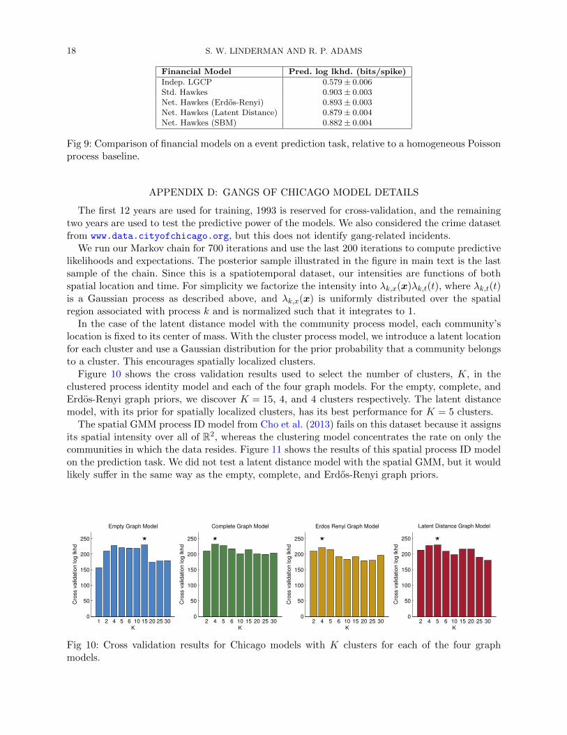
The first 12 years are used for training, 1993 is reserved for cross-validation, and the remainingtwo years are used to test the predictive power of the models. We also considered the crime datasetfrom www.data.cityofchicago.org, but this does not identify gang-related incidents.

We run our Markov chain for 700 iterations and use the last 200 iterations to compute predictivelikelihoods and expectations. The posterior sample illustrated in the figure in main text is the lastsample of the chain. Since this is a spatiotemporal dataset, our intensities are functions of bothspatial location and time. For simplicity we factorize the intensity into λk,x(x)λk,t(t), where λk,t(t)is a Gaussian process as described above, and λk,x(x) is uniformly distributed over the spatialregion associated with process k and is normalized such that it integrates to 1.

In the case of the latent distance model with the community process model, each community’slocation is fixed to its center of mass. With the cluster process model, we introduce a latent locationfor each cluster and use a Gaussian distribution for the prior probability that a community belongsto a cluster. This encourages spatially localized clusters.

Figure 10 shows the cross validation results used to select the number of clusters, K, in theclustered process identity model and each of the four graph models. For the empty, complete, andErdos-Renyi graph priors, we discover K = 15, 4, and 4 clusters respectively. The latent distancemodel, with its prior for spatially localized clusters, has its best performance for K = 5 clusters.

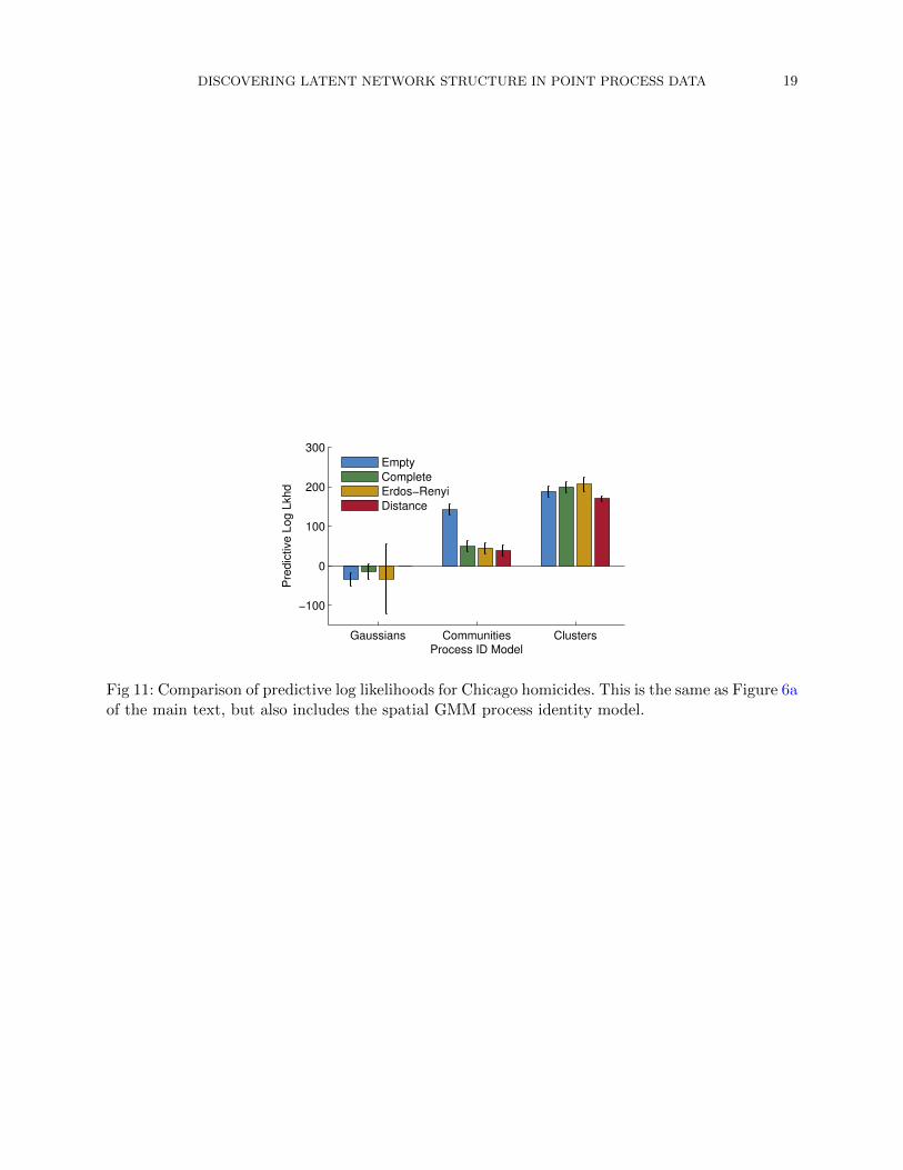
The spatial GMM process ID model from Cho et al. (2013) fails on this dataset because it assignsits spatial intensity over all of R2, whereas the clustering model concentrates the rate on only thecommunities in which the data resides. Figure 11 shows the results of this spatial process ID modelon the prediction task. We did not test a latent distance model with the spatial GMM, but it wouldlikely suffer in the same way as the empty, complete, and Erdos-Renyi graph priors.

1 2 4 5 6 10 15 20 25 300

50

100

150

200

250

K

Cro

ss v

alid

ation log lkhd

Empty Graph Model

2 4 5 6 10 15 20 25 300

50

100

150

200

250

K

Cro

ss v

alid

ation log lkhd

Complete Graph Model

2 4 5 6 10 15 20 25 300

50

100

150

200

250

K

Cro

ss v

alid

ation log lkhd

Erdos Renyi Graph Model

2 4 5 6 10 15 20 25 300

50

100

150

200

250

K

Cro

ss v

alid

ation log lkhd

Latent Distance Graph Model

Fig 10: Cross validation results for Chicago models with K clusters for each of the four graphmodels.

www.data.cityofchicago.org


Gaussians Communities Clusters

−100

0

100

200

300

Process ID Model

Pre

dic

tive

Lo

g L

kh

d

Empty

Complete

Erdos−Renyi

Distance

Fig 11: Comparison of predictive log likelihoods for Chicago homicides. This is the same as Figure 6aof the main text, but also includes the spatial GMM process identity model.

discovering latent network structure in point … latent network structure in point process ......

Documents