discounting and compounding - city university …€¦ · ppt file · web view ·...

1

Lecture: Valuing Companies andInvestment Projects

This version 11/9/2001. Includes WORD tables

Copyright K. Cuthbertson and D. Nitzsche

2

TOPICS

Basic Ideas

Compounding/Terminal Value

Discounted Present Value DPV \ Discounted Cash Flow DCF

Investment ( Project) Appraisal, Internal Rate Of Return,

Valuation Of The Firm: Enterprise Vale and Equity

~ choice of discount rate

~ valuation in practice: EBITD, Depreciation, FCF etc.

Complementary Valuation Techniques: EP, EVA,APV

Self Study: Other Investment Appraisal Methods


3

READING

Investments:Spot and Derivative Markets, K.Cuthbertson and D.Nitzsche

Chapter 3Discounted Present Value DPV \ Discounted Cash Flow DCF

Internal Rate Of Return, IRR

Investment ( Project) Appraisal

Valuation Of The Firm And The Firm’s Equity (Incl. Continuing Value).

Valuation In Practice: EBITD, Depreciaiton, FCF etc

Other Investment Appraisal Methods

Chapter 11Economic Profit, Economic Value Added, Adjusted Present Value

P. 342-346.


4

BASIC IDEAS

Compounding/Terminal ValueDiscounted Present Value DPV

Discounted Cash Flow DCF Internal Rate of Return

Investment/ Project Appraisal


5

Compounding/ Terminal Value

Assume zero inflation+cash flows known with certainty

Vo = value today ($1000), r = interest rate (0.10)

Value in 1,2 years time

V1 = (1.1) 1000 = $1100

V2 = (1.1) 1100 = (1.1) 2 1000 = $1210

Terminal Value after n-years: Vn = Ao (1 + r)n

We could ‘move all payments forward’ to time n=10 years and then add them - but we do not do this


6

Discounting

‘Bring all payments back’ to t=0 and then add.

Value today of V2 = $1210 payable in 2 yrs ?

DPV =

Hence “ DPV of $1210 is $1000”

Which means that $1000 today is equivalent to $ 1210 payable in 2-years

“Discount Factor” d2 =

Vr2

2 21121011( ) ( . )

11 2( )r


7

Discounted Present Value (DPV)

What is value today of stream of payments - usually called ‘Cash Flows’, assuming a constant discount factor? :

DPV = = d1 V1 + d2 V2 + ..

r = ‘discount rate’

d = “discount factor” < 1

Discounting, puts all future future cash flows on to a ‘common cash flows on to a ‘common time’ at t=0 - so they can then be “added up”.time’ at t=0 - so they can then be “added up”.

Vr

Vr

1 221 1( ) ( )

...


8

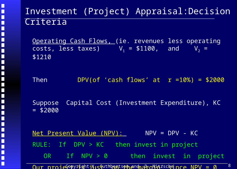
Operating Cash Flows, (ie. revenues less operating costs, less taxes) V1 = $1100, and V2 = $1210

Then DPV(of ‘cash flows’ at r =10%) = $2000

Suppose Capital Cost (Investment Expenditure), KC = $2000

Net Present Value (NPV): NPV = DPV - KC

RULE: If DPV > KC then invest in project

OR If NPV > 0 then invest in project

Our project is just ‘on the margin’ since NPV = 0 when r=10%

Investment (Project) Appraisal:Decision Criteria


9

r=5

NPV

r= loan rate or discount rate

NPV=145

r=10

If r <10% then you would invest in the projectIf r > 10% you would NOT invest in the projectNPV=0

NPV (for given CFs) and the cost of borrowing, r


10

Businessmen think in terms the rate of return on the projectWhat is the rate of return (on capital investment of $2000) ?

It is the rate of return which gives NPV = 0 Hence the IRR is the ‘break-even’ discount rate and IRR = 0.10 (10%)

IRR INVESTMENT DECISION RULE

Invest in project if : IRR > cost of borrowing, r

Internal Rate Of Return (IRR)

02000)1(

1210)1(

11002

IRRIRR


11

If NPV = 0 OR, IRR = cost of borrowing then this implies

-the CF from the project will just pay off all the annual interest payments on the loan + the principal amount borrowed from the bank

Note: Internal funds are not ‘free’

Intuitively what do NPV and IRR rules mean ?


12

KC=2000 (borrowed at r=10%), CF are V1=1100 , V2=1210

Year 1 Year 2

LoanOutstanding

2200 =2000(1.1)

1210 = 1100 ( 1.1 )

NetReceipts 1100 1210AmountOwed 1100 0

Payoff all interest and principal if NPV=0 or IRR = 10% ?


Intuitively what do NPV and IRR rules mean ?

13

Valuation of the Firm:

Enterprise Value and Equity Value


14

General CaseGeneral Case

VV00 = FCF = FCF11 / (1+r) + FCF / (1+r) + FCF22 / ((1+r) / ((1+r)22 + …… + ……

FCF= Free Cash FlowsFCF= Free Cash Flows

1) Sum to infinity and FCF is constant:1) Sum to infinity and FCF is constant:

VV00 = FCF / r = FCF / r

2) Sum to infinity and FCF grows at rate of g % p.a. 2) Sum to infinity and FCF grows at rate of g % p.a. (g=0.05 )(g=0.05 )

VV00 = FCF = FCF11 / ( r - g) / ( r - g)

Two Useful Math Results


15

Enterprise DCFEnterprise DCF

In practice investment costs occur every year so:In practice investment costs occur every year so:

V(whole firm) = DPV ( Free Cash Flows, FCF)V(whole firm) = DPV ( Free Cash Flows, FCF)

FCF = (Operating ‘cash flows’ - Gross investment) FCF = (Operating ‘cash flows’ - Gross investment) each yearyear

Value of EquityValue of Equity

V(Equity) = V(whole firm) - V(Debt outstanding)V(Equity) = V(whole firm) - V(Debt outstanding)

‘‘Fair value for one share’ = V(Equity) / N Fair value for one share’ = V(Equity) / N

N = no. of shares outstanding (+ ‘minority interests’)N = no. of shares outstanding (+ ‘minority interests’)

‘Enterprise Value’ and ‘Equity Value’


16

In an In an efficient marketefficient market the price of the the price of the share(s) should equal ‘fair value’share(s) should equal ‘fair value’

We will learn how to value corporate We will learn how to value corporate debt, in later lecturesdebt, in later lectures

‘Enterprise Value’ and Equity Value


17

The DPV of ALL the firm’s future cash flows is The DPV of ALL the firm’s future cash flows is often ‘split’ into two (or more) planning horizons:often ‘split’ into two (or more) planning horizons:

‘‘ENTERPRISE DCF’ENTERPRISE DCF’

= DPV of FCF in years 1-5 = DPV of FCF in years 1-5

+ DPV of ‘Continuing Value’ after year-5+ DPV of ‘Continuing Value’ after year-5

‘Valuing the ‘Firm’ :Continuing Value


18

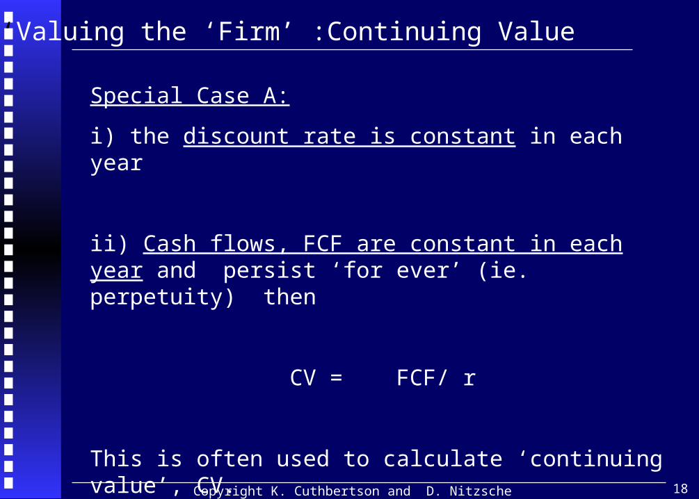
Special Case A:

i) the discount rate is constant in each year

ii) Cash flows, FCF are constant in each year and persist ‘for ever’ (ie. perpetuity) then

CV = FCF/ r

This is often used to calculate ‘continuing value’, CV.



19

eg. Project has

V5 =100 in year-5,6,7 etc., and r=0.10 then

Continuing value CV (at t=5) = 100 / 0.10 = 1,000

and

DPV (at t=0) of the CV = 1000/ (1+r)5 = 621



20

Special Case B:

If

i) the discount rate is constant in each year

and

ii)FCF’s grow at a constant rate each year, say after year-5 then

CV (at t=5) = FCF5 (1+g) / ( r - g) for r>g



21

Project has FCF=100 in year-5

FCF grows at rate g=0.03 (3%) and r = 0.10

Then:

Continuing value CV (at t=5)

= 100 (1.03) / (0.10 - 0.03)= 1471

DPV( at t=0) of the CV = 1471/ (1+r)5 = 913

Notes:

CV is very sensitive to the choices made for FCF5, R and g.

CV can be a large & dominates DPV of the cash flows over years 1-5.



22

Suppose

Value of firm using DPV of FCF’s is

Enterprise DCF = DPV (FCF 1-5yrs) + DPV (of CV)

= 679 + 621 = 1,300

Suppose: All equity financed firm N = 1000 shares and P= $1

Market Value (Capitalisation) = $1000

Hence the shares are undervalued by 30%

Possible purchase or takeover target (by ‘arbs’)

Company Valuation: M&A


23

If NPV of the project > 0 (discounted using RS)

Implies the managers are ‘adding value’ for shareholders (which exceeds the return they could earn from investing their money in other hamburger firms).

This is value based management or ‘creating shareholder value’.

Shareholder Value (All equity financed firm)


24

Choice of Discount Rate


25

Note: ‘All equity’ financed = ‘unlevered firm’ - ie. no debt

Discount rate should reflect ‘business risk’ of the project.

Assume project is ‘scale enhancing’ (eg. more hamburger outlets for McDonalds)

Hence, has same ‘business risk’ as the firm as a whole.

Simple method

Use the average (historic) return on equity, RS (e.g. 15%) for this (hamburger) firm as the discount rate

This assumes the observed return on equity correctly reflects the payment for risk, that shareholders require from this hamburger company.

Discount Rate: All equity financed firm


26

If the project being considered by MacDonalds is to build hotels, then we would use the average stock market return in “hotel sector” (20%pa. say)

- as this reflects the “required return on equity capital” for the shareholders in that sector.

- see CAPM / SML / APT later, where we provide more sophisticated methods for choosing the appropriate equity discount rate.


Discount Rate: All equity financed firm

27

Levered firm = financed by mix of debt and equity Assume debt-equity ratio will remain broadly unchanged after the

new project is completed.

Then discount FCF using:

(‘After tax’)Weighted Average Cost of Capital WACC, WACC = (1-z) RS + z RB (1-t)

z = B / V = propn of debt(bonds) , (1-z) = S / V V=market value of firm = S+B ‘weights’, z, sum to 1.


Discount Rate: levered firm

28

S = market value of outstanding equity ( = N x stock price)

B = market value of outstanding debt (ie. bonds issued and bank loans)

RS = average return on equity in hamburger industry

RB = interest rate (yield to maturity) on say 10-year corp. AA-rated bonds(If hamburger company is rated AA by S&Poor’s)

t = corporate tax rate

Note: Market value (‘cap’) of the firm V = S +B


Discount Rate: levered firm

29

Assume firm is part-equity financed and part-debt financed

Then the ‘intrinsic value’ of the firm is the DPV of its future cash flows from all of its current and future investment projects, discounted using WACC

Managers can only increase the value of the firm by1) investing in projects with ‘high’ FCFs2) reducing the WACC

‘(2)’ is the so-called capital structure question - can managers change the mix of debt and equity financing to lower the overall WACC? - assuming FCF is unchanged - see Modigliani-Miller later

Can Managers Increase the Value of the Firm?


30

1) Key practical method is to use “sensitivity” or “scenario” analysis.

Sensitivity - ‘one at a time’1) What is NPV if revenues are much higher/lower ? 2) What is the NPV if the discount rate is 1% higher?Scenario:3) What is the NPV if both (1) and (2) apply. - scenario analysis(Monte Carlo simulation is a sophisticated way of doing this)

Can “include” probabilities in (1) and hence calculate EXPECTED NPV and its standard deviation.

What about (business) risk in DCF ?


31

2) Can use decision trees - particularly useful where there are strategic options in the investment decision

-eg. Suppose you can abandon the project and sell the ‘plant’ for $10m if demand turns out to be ‘low’ in year-2. On the other hand if demand is ‘high’ then you will continue production in year-2.

This affects the NPV of the project compared with the ‘normal case’ where you assume you do not abandon

In fact the ‘correct’ way to evaluate these strategic options is (not surprisingly) to use ‘real options theory’, but this cannot be done here !

What about (business) risk in DCF ?


32

VALUATION IN PRACTICE:

EBITD, DEPRECIAITON, FCF


33

ACCOUNTING NIGHTMARES

Earnings before interest, tax and depreciation,EBITD

EBITD = R - C = Sales Revenues - Operating Costs (Labour+Materials)

Free Cash Flow FCF= (R - C - T) - Inv(gross) - Increase in WC + (Net Non-Op. Inc)

Valuing a Company: ‘Cash is King’

Calculating ‘Free Cash Flow’ in Practice


34

Now the Accountants ‘Mess it About’ Published ‘Earnings’ or ‘profit’ are usually presented after a deduction for

depreciation: These would be ‘earnings before interest and tax’ EBIT

So, EBIT = EBITD - D = (R-C) - D

Hence, to get FCF ‘add back’ depreciation and deduct taxes:FCF =(EBIT - T) + D - Inv(gross) - Increase in WC +(N.N.Op.Inc)

Also, you often ‘see’ (in the UK):

Net Op. Profit (Less Taxes) NOPLAT = EBIT - T = R-C-D-T

Valuing a Company: ‘Cash is King’


35

Valuing a Company

CASH IS KING

Table 3.7 : CAPITAL ACCOUNT

Year-0

Year-1

Year-2

Year-3

Year-4

Year-5

1. Capital Cost, KC 1,0002. Depreciation(1.)

(= KC – SV)/n200 200 200 200 200

3. AccumulatedDepreciation(=”sum ofdepreciation”)

200 400 600 800 1,000

4. Year End Book Value(= 4 – 3)

1,000 800 600 400 200 0

5. Working Capital, WC 0 400 500 600 500 2006. Total Book Value

(= 4 + 5)1,000 1,200 1,100 1,000 700 200

7. Change in WorkingCapital,. WC(= WCt – WCt-1)

400 100 100 (100) (300)

Notes: 1. Total capital cost is KC = $1,000. Scrap value SV = 0 at n=5 years.Hence D = (KC – SV)/5 = 200 per year (straight line depreciation).

2. ( . ) indicates a negative number


36

Valuing a Company

Table 3.8 : DEPRECIATION AND TAX

Year-1

Year-2

Year-3

Year-4

Year-5

1. Sales revenue, R 1,000 1,500 2,000 2,500 3,0002. Labour + Materials

Cost, C600 900 1,200 1,500 1,800

3. EBITD(1.) (= 1 – 2) 400 600 800 1,000 1,200

4. Depreciation, D 200 200 200 200 2005. Earnings after

Depreciation,= R – C – D (= 3 – 4)

200 400 600 800 1,000

6. Tax(2.)

= 0.30(R – C – D)60 120 180 240 300

ote : 1. EBITD = earnings before interest, tax and depreciation. Accounting profits (before tax)reported in the ‘income-expenditure’ (or ‘profit-loss’) account would be (EBITD – D).

2. Corporate tax rate is assumed to be t = 0.30 (30%).


37

Table 3.9 : CALCULATING FREE CASH FLOW

Year-1

Year-2

Year-3

Year-4

Year-5

1. Sales revenue(1.), R 1,000 1,500 2,000 2,500 3,0002. Labour + Material Cost(1.) 600 900 1,200 1,500 1,8003. Earnings before Interest,

Tax and Depreciation,EBITD(= 1 – 2)

400 600 800 1,000 1,200

4. Tax(1.), T 60 120 180 240 3005. After Tax Operating Cash

Flow(= 3 – 4)

340 480 620 760 900

6.Increase in WorkingCapital(2.), WC

400 100 100 (100) (300)

7. Capital Cost, KC (GrossInvestment Expenditure)(3.)

600 400 0 0 0

8. Operating Cash Flow (after tax)(= 5 – 6 – 7)

(660) (20) 520 860 1,200

9. Cash flow from Non-operating assets(6)

50 0 0 100 0

10.

After tax Interest Incomefrom Assets

10 15 20 15 10

11.

Decrease (Increase) inMarketable Securities

0 (10) 20 15 (10)

12.

Free Cash Flow(4.), FCF(= 8 + 9 + 10 + 11)

(600) (15) 560 990 1,200

Note : 1. Figures are from table 3.8.2. An increase in working capital is a cash outflow. Figures are from

table 3.7 (row 7).3. These are the actual cash expenditures on investment in each year

and they sum to the total capital cost KC (in table 3.7).4 Cash flow available to investors (ie. debt holders and equity

holders). Note that some forecasts of FCF might exclude items 9and 10.

5 ( . ) indicates a negative number6 e.g. sale of a subsidiary,


38

Valuing a Company

Table 3.10 : USE OF FREE CASH FLOW OF THE FIRM

Year-1

Year-2

Year-3

Year-4

Year-5

1. Free Cash Flow(table 3.9, row 12)

-600 -15 560 990 1,200

FINANCING (USE OF FREE CASH FLOWS)2. Interest Paid to Debtholders 30 30 30 30 303. Dividends Paid 100 105 110 115 1204. Change in Share Capital

+ = repurchases(..) = new issues

100 100 100 100 100

5. Change in Net DebtOutstanding+ = decrease,(.. ) = increase

(830) (250) 320 745 950

Total Financing(= 2 + 3 + 4 +5)

-600 -15 560 990 1,200


39

Complementary Valuation Techniques:

Economic Profit, EP

Economic Value Added, EVA

Adjusted Present Value, APV


40

EP and EVA are equivalent to ‘Enterprise DCF’ if the calculationsare done consistently -ie. before the accountants get at the figures

ECONOMIC PROFIT (McKinsey and Co)

EP = ( ROC - WACC) x Capital Stock, K

where Return on Capital, ROC = ‘Profit’ / K

If ROC > WACC then the managers chosen investment projects are earning a rate of return in excess of WACC and therefore, the investment projects are ‘Adding value’.

Economic Profit


41

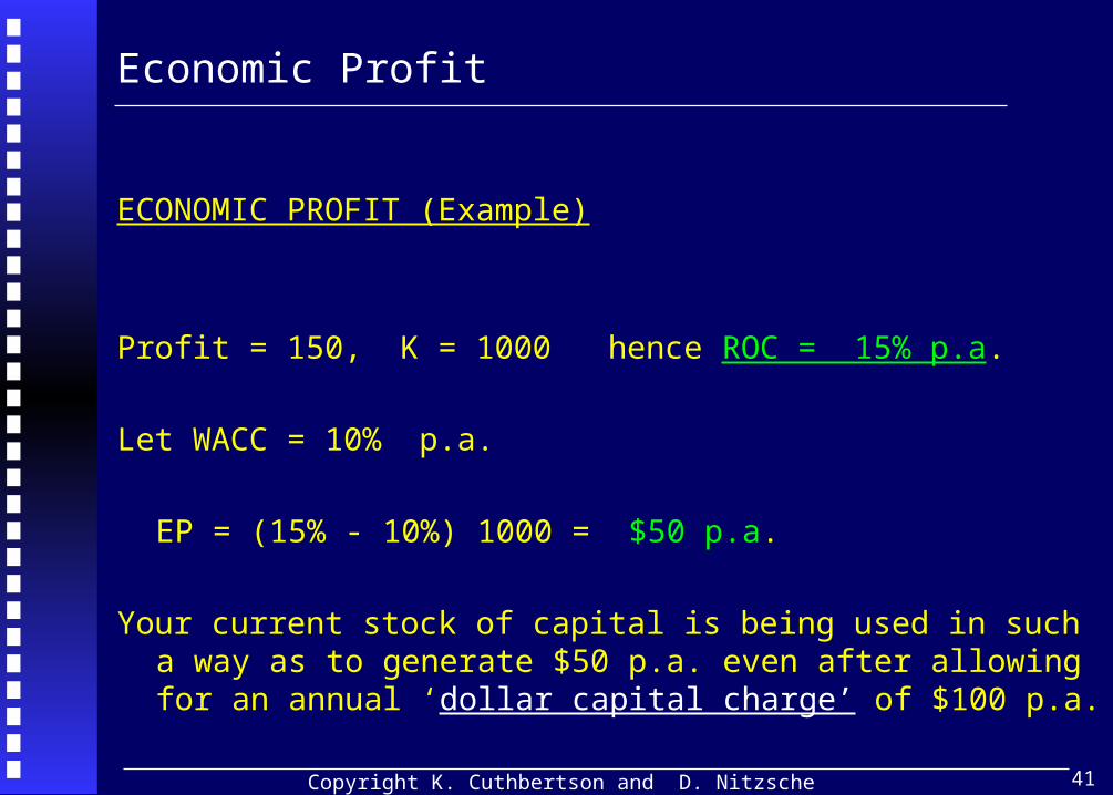
ECONOMIC PROFIT (Example)

Profit = 150, K = 1000 hence ROC = 15% p.a. Let WACC = 10% p.a.

EP = (15% - 10%) 1000 = $50 p.a.

Your current stock of capital is being used in such a way as to generate $50 p.a. even after allowing for an annual ‘dollar capital charge’ of $100 p.a.

Economic Profit


42

EVA= ‘Profit’ - ‘Capital Charge’ = 150 - (10%)1000 = $50 p.a.

where ‘Capital charge’ = WACC x ‘Adjusted Capital’, K

EVA is equivalent to EP if we measure ‘profit’ and ‘capital’ in the same way, for both techniques.

eg. do we ‘add back’ to ‘capital’ past R&D expenditures on the grounds that this outlay increased ‘knowledge’ which is an ‘asset’

Economic Value Added, EVA


43

You can compare different firms’ performance on EP and EVA in any one year (or over several years).

The ‘plus’, compared to using say just ‘profits’ or ROC is that EP and EVA assess ‘profit’ in relation to ‘the cost of capital’.

Value of the firm (at t=0 ) using EP or EVA

= (Net) Capital Stock at t=0, K0

+ DPV ( of EP or EVA p.a., ~ WACC as discount rate)

EP and EVA


44

Simple proof that ‘Enterprise DCF’ and EP or EVA are equivalent:

Assume K0 = 1000 (no depreciation), ROC = 15%, ‘Profit’ = 150 (perpetuity)

1) ‘Enterprise DCF = ‘Profit’ / WACC = 150/0.10 = $1500

2) EP or EVA: EP = (15% - 10%) 1000 = $50 p.a.

3) V(firm) = K0 + EP / WACC = 1000 + 50 / 0.10 = $1500

SELF STUDYComplementary Valuation Techniques:


45

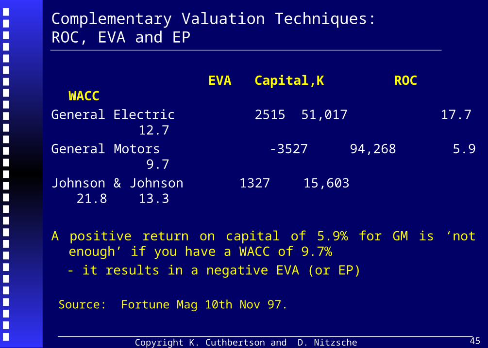
EVA Capital,K ROC WACC

General Electric 2515 51,017 17.7 12.7General Motors -3527 94,268 5.9 9.7Johnson & Johnson 1327 15,603 21.8 13.3

A positive return on capital of 5.9% for GM is ‘not enough’ if you have a WACC of 9.7%

- it results in a negative EVA (or EP)

Source: Fortune Mag 10th Nov 97.

Complementary Valuation Techniques: ROC, EVA and EP


46

When using ‘Enterprise DCF’ we discounted the FCF using ‘after tax’ WACC

Our measure of FCF did not contain any ’tax offsets/shields’ on (debt) interest payments (the only tax offsets we considered were on depreciation).

This was because these ‘tax offsets’ are taken care of in the denominator, the WACC, which is reduces the cost of debt to Rb(1-t).

APV and Enterprise DCF give the same value for the firm if consistent measures of the cost of equity and debt are used. This is a difficult area which we cannot pursue here but note that

APV = FCF discounted as if firm is all-equity + DPV of ‘tax offsets’ See Copeland, T. Koller, T and Murrin, J. Valuation (J. Wiley) for the best practical

account of this and other valuation issues.

Adjusted Present Value, APV(Not Examinable)


47

END OF LECTURE

SELF STUDY SLIDES FOLLOW


48

1) SOME PATHOLOGICAL CASES ~ COMPLICATIONS WITH IRR !

2) OTHER METHODS USED IN INVESTMENT APPRAISAL

(These are of minor importance but you should be aware of these issues)

SELF STUDY


49

Table 2: ‘DIFFERENT CASH FLOW PROFILES

Project A (-100, 130)Project B (100, - 130)Project C (-100, 230, - 132)

-------------------------------------------------------------Project A ~ ‘normal’Project B ~ ‘Rolling Stone’s Concert’Project C ~ ‘Open cast mining’

-------------------------------------------------------------IRR gives wrong decision for B and CNPV gives correct decision for A,B,CANSWER: Use NPV !

Complications: Mainly with IRR !


50

Mutually exclusive projects(eg. garage or hamburger joint on one site, BUT NOT BOTH)

- use NPV not IRR criterion(afficionados could use the incremental-IRR criterion ! )

Capital Constraint (ie. not enough funds for all projects with NPV>0)- rank projects by the ‘profitability index’, PI where:

PI = ( NPV / Capital Cost) = “bang per buck”

Choose those projects with largest PI values until you exhaust your funds.

Complications: Mainly with IRR !


51

Year-0 Year-1 Year-2 Year-3 Year-4

FV -1000 500 500 700 0d 1.0 0.8696 0.7561 0.4972 -

PV -1000 435 378 348 -

Note: NPV = 161

1) Payback Period = 2 years2) Discounted Payback = 2-3 years

Investment Appraisal: Alternative Methods


52

Either

Ignores cash flows after payback period (eg. never invest in ‘Dolly the sheep’)

OR

Ignores time value of money

Deficiencies: Alternative Methods


53

END OF SLIDES


discounting and compounding - city university …€¦ · ppt file · web view ·...

Documents