discontinuous superprocesses with dependent spatial motion
TRANSCRIPT

Stochastic Processes and their Applications 119 (2009) 130–166www.elsevier.com/locate/spa
Discontinuous superprocesses with dependentspatial motionI
Hui He
Laboratory of Mathematics and Complex Systems, School of Mathematical Sciences, Beijing Normal University,Beijing 100875, People’s Republic of China
Received 25 April 2007; received in revised form 3 January 2008; accepted 4 February 2008Available online 16 February 2008
Abstract
We construct a class of discontinuous superprocesses with dependent spatial motion and generalbranching mechanism. The process arises as the weak limit of critical interacting–branching particlesystems where the spatial motions of the particles are not independent. The main work is to solve themartingale problem. When we turn to the uniqueness of the process, we generalize the localizationmethod introduced by [Daniel W. Stroock, Diffusion processes associated with Levy generators,Z. Wahrscheinlichkeitstheorie und Verw. Gebiete 32 (1975) 209–244] to the measure-valued context. Asfor existence, we use particle system approximation and a perturbation method. This work generalizes themodel introduced in [Donald A. Dawson, Zenghu Li, Hao Wang, Superprocesses with dependent spatialmotion and general branching densities, Electron. J. Probab. 6 (25) (2001) 33 pp (electronic)] where aquadratic branching mechanism was considered. We also investigate some properties of the process.c© 2008 Elsevier B.V. All rights reserved.
MSC: primary 60J80; 60G57; secondary 60J35
Keywords: Measure-valued process; Superprocess; Dependent spatial motion; Interaction; Localization procedure;Duality; Martingale problem; Semi-martingale representation; Perturbation; Moment formula
1. Introduction
Notation: For the reader’s convenience, we introduce here our main notation. Let R denotethe one-point compactification of R. Let Rn denote the n-fold Cartesian product of R. LetM(R) denote the space of finite measure endowed with the topology of weak convergence.
I Supported by NSFC (No. 10121101).E-mail address: h hui [email protected].
0304-4149/$ - see front matter c© 2008 Elsevier B.V. All rights reserved.doi:10.1016/j.spa.2008.02.002

H. He / Stochastic Processes and their Applications 119 (2009) 130–166 131
We denote by λn the Lebesgue measure on Rn . Given a topological space E , let B(E) denotethe Borel σ -algebra on E . Let B(E) denote the set of bounded measurable functions on E andlet C(E) denote its subset comprising bounded continuous functions. Let C(Rn) be the space ofcontinuous functions on Rn which vanish at infinity and let C∞c (Rn) be functions with compactsupport and bounded continuous derivatives of any order. Let C2(Rn) denote the set of functionsin C(Rn) which are twice continuously differential functions with bounded derivatives up tothe second order. Let C2
c (Rn) denote the set of functions in C2(Rn) with compact support. LetC2(Rn) be the subset of C2(Rn) of functions that together with their derivatives up to the secondorder vanish at infinity.
Let
C2∂ (R
n) = f + c : c ∈ R and f ∈ C2(Rn)
and
C20(R
n) = f : f ∈ C2∂ (R
n) and (1+ |x |2)Dα f (x) ∈ C(Rn), α = 1, 2,
where D1 f =∑n
i=1 |∂ f/∂xi | and D2 f =∑n
i, j=1 |∂2 f/∂xi∂x j |. We use the superscript “+”
to denote the subsets of non-negative elements of the function spaces, and “++” is used todenote the subsets of non-negative elements bounded away from zero, e.g., B(Rn)+, C(Rn)++.Let f i denote the first-order partial differential derivatives of the function f (x1, . . . , xn) withrespect to xi and let f i j denote the second-order partial differential derivatives of the functionf (x1, . . . , xn) with respect to xi and x j . We denote by C ([0,∞), E) the space of continuouspaths taking values in E . Let D ([0,∞), E) denote the Skorokhod space of cadlag paths takingvalues in E . For f ∈ C(R) and µ ∈ M(R) we shall write 〈 f, µ〉 for
∫f dµ.
A class of superprocesses with dependent spatial motion (SDSM) over the real line R wereintroduced and constructed in [18,19]. A generalization of the model was then given in [4]. Wefirst briefly describe the model constructed in [4]. Suppose that c ∈ C2(R) and h ∈ C(R) issquare-integrable. Let
ρ(x) =∫R
h(y − x)h(y)dy, (1.1)
and a(x) = c(x)2 + ρ(0) for x ∈ R. We assume in addition that ρ ∈ C2(R) and |c| is boundedaway from zero. Let σ be a non-negative function in C2(R) that can be extended continuously toR. Given a finite measure µ on R, the SDSM with parameters (a, ρ, σ ) and initial state µ is theunique solution of the (L, µ)-martingale problem, where
L F(µ) := A F(µ)+ B F(µ), (1.2)
A F(µ) :=12
∫R
a(x)d2
dx2
δF(µ)
δµ(x)µ(dx)
+12
∫R2ρ(x − y)
d2
dxdy
δ2 F(µ)
δµ(x)δµ(y)µ(dx)µ(dy), (1.3)
B F(µ) :=12
∫Rσ(x)
δ2 F(µ)
δµ(x)2µ(dx), (1.4)
for some bounded continuous functions F(µ) on M(R). The variational derivative is defined by
δF(µ)
δµ(x)= lim
r→0+
1r[F(µ+ rδx )− F(µ)], x ∈ R, (1.5)

132 H. He / Stochastic Processes and their Applications 119 (2009) 130–166
if the limit exists and δ2 F(µ)/δµ(x)δµ(y) is defined in the same way with F replacedby (δF/δµ(y)) on the right hand side. Clearly, the SDSM reduces to a usual criticalDawson–Watanabe superprocess if h(·) ≡ 0 (see [2]). A general SDSM arises as the weaklimit of critical interacting–branching particle systems. In contrast to the usual branching particlesystem, the spatial motions of the particles in the interacting–branching particle system are notindependent. The spatial motions of the particles can be described as follows. Suppose thatW (t, x) : x ∈ R, t ≥ 0 is space–time white noise based on the Lebesgue measure, the commonnoise, and Bi (t) : t ≥ 0, i = 1, 2, . . . is a family of independent standard Brownian motions,the individual noises, which are independent of W (t, x) : x ∈ R. The migration of a particle inthe approximating system with label i is defined by the stochastic equations
dxi (t) = c(xi (t))dBi (t)+∫R
h(y − xi (t))W (dt, dy), t ≥ 0, i = 1, 2, . . . , (1.6)
where W (dt, dy) denotes the time–space stochastic integral relative to Wt (B). For each integerm ≥ 1, (x1(t), . . . , xm(t)) : t ≥ 0 is an m-dimensional diffusion process which is generatedby the differential operator
Gm:=
12
m∑i=1
a(xi )∂2
∂x2i
+12
m∑i, j=1,i 6= j
ρ(xi − x j )∂2
∂xi∂x j. (1.7)
In particular, xi (t) : t ≥ 0 is a one-dimensional diffusion process with generator G :=(a(x)/2)∆. Because of the exchangeability, a diffusion process generated by Gm can be regardedas an interacting particle system or a measure-valued process. Heuristically, a(·) represents thespeed of the particles and ρ(·) describes the interaction between them. The diffusion processgenerated by A arises as the high density limit of a sequence of interacting particle systemsdescribed by (1.6); see Wang [18,19] and Dawson et al. [4]. There are at least two differentways to look at the SDSM. One is as a superprocess in random environment and the other is asan extension of models of the motion of the mass with stochastic flows (see [13]). Some otherrelated models were introduced and studied in Skoulakis and Adler [15]. The SDSM possessesproperties very different from those of the usual Dawson–Watanabe superprocess. For example,a Dawson–Watanabe superprocess in M(R) is usually absolutely continuous whereas the SDSMwith c(·) ≡ 0 is purely atomic; see Konno and Shiga [10,3,20], respectively.
To best of our knowledge, in all of the work which considered the SDSM and related modelsonly continuous processes have been introduced and studied. In this paper, we construct a classof discontinuous superprocesses with dependent spatial motion. A modification of the abovemartingale problem is to replace operator B in (1.2) by
B F(µ) =12
∫Rσ(x)
δ2 F(µ)
δµ(x)2µ(dx)
+
∫Rµ(dx)
∫∞
0
(F(µ+ ξδx )− F(µ)−
δF(µ)
δµ(x)ξ
)γ (x, dξ), (1.8)
whose coefficients satisfy
(i) σ ∈ C2∂ (R)
+,
(ii) γ (x, dξ) is a kernel from R to (0,+∞) such that supx [∫+∞
0 ξ ∧ ξ2γ (x, dξ)] < +∞,
(iii)∫Γ ξ ∧ ξ
2γ (x, dξ) ∈ C2∂ (R) for each Γ ∈ B((0,∞)).

H. He / Stochastic Processes and their Applications 119 (2009) 130–166 133
A Markov process generated by L is a measure-valued branching process with branchingmechanism given by
Ψ(x, z) :=12σ(x)z2
+
∫∞
0(e−zξ
− 1+ zξ)γ (x, dξ).
This process is naturally called a superprocess with dependent spatial motion (SDSM) withparameters (a, ρ,Ψ). This modification is related to the recent work of Dawson et al. [4], whereit was assumed that γ (x, dξ) = 0. Though our model is an extension of the model introduced inWang [18,19] and Dawson et al. [4], the construction of our model differs from that of theirs. Wedescribe our approach to the construction of our model in the following.
The main work of this paper is to solve the (L, µ)-martingale problem. As for uniqueness,following the idea of Stroock [16] a localization procedure is developed. Therefore, we donot consider the (L, µ)-martingale problem directly. Instead, we will first solve the (L′, µ)-martingale problem, where
L′F(µ) := A F(µ)+ B′F(µ), (1.9)
B′ :=12
∫Rσ(x)
δ2 F(µ)
δµ(x)2µ(dx)−
∫Rµ(dx)
∫∞
l
δF(µ)
δµ(x)ξγ (x, dξ)
+
∫Rµ(dx)
∫ l
0
(F(µ+ ξδx )− F(µ)−
δF(µ)
δµ(x)ξ
)γ (x, dξ) (1.10)
and we make the convention that∫ l
0=
∫(0,l)
and∫∞
l=
∫[l,∞)
for 0 < l < ∞. We regard the (L′, µ)-martingale problem as the ‘killed’ martingale problem.We shall see that the Markov process associated with the ‘killed’ martingale problem also arisesas high density limit of a sequence of interacting–branching particle systems and it is an SDSMwith branching mechanism given by
Ψ0(x, z) :=12σ(x)z2
+
∫∞
lξγ (x, dξ)z +
∫ l
0(e−zξ
− 1+ zξ)γ (x, dξ).
It is easy to see from the branching mechanism that the process is a subcritical branching processwhere all ‘big’ jumps such that the jump size is larger than l have been ‘killed’. We will use aduality method to show the uniqueness of the ‘killed’ martingale problem. We shall construct adual process and show its connection with the solutions of the ‘killed’ martingale problem whichgives the uniqueness. When we establish the dual relationship, we point out that there exists agap in the proof for establishing the dual relationship in [4]; see Remark 2.2 in Section 2 of thispaper for details. Then a localization argument is developed to show that if the (L′, µ)martingaleproblem is well-posed then uniqueness holds for the (L, µ)-martingale problem. The argumentconsists of three parts.
In the first part, we show that each solution of the (L, µ)-martingale problem, say X , behavesin the same way as the solution of the killed martingale problem until it has a ‘big jump’ whosejump size is larger than l. Intuitively, one can think of the branching particle system as follows.In the branching particle system corresponding to the (L, µ)-martingale problem, if a particledies and it leaves behind a large number of offspring, say more than 500, which will always beregarded as a ‘big jump’ event, we kill all of its offspring. Then we get a new branching particle

134 H. He / Stochastic Processes and their Applications 119 (2009) 130–166
system and before the jump event happens the two systems are the same. The evolution of thenew particle system represents the behavior of the solution to the ‘killed’ martingale problem.It is clear that if the original branching particle system is a critical system, the new particlesystem is a subcritical branching system. Since the ‘killed’ martingale problem is well-posed, Xis uniquely determined before it has a ‘big jump’. Next, we show that when a ‘big jump’ eventhappens, the jump size is uniquely determined. This conclusion is not surprising either. Givena branching mechanism, in a branching particle system, when a particle dies, the distribution ofits offspring number is uniquely determined by the position of the particle itself (we assume thatthe branching mechanism is independent of time). Thus we can find a predictable representationfor the jump size. According to the argument in the first part, we see the jump size is uniquelydetermined. Finally, we can prove by induction that the distribution of X is uniquely determined,since after the first ‘big jump’ event happens, X also behaves in the same way as the solutionof the ‘killed’ martingale problem until the second ‘big jump’ event happens. Before we use thelocalization procedure, we follow an argument taken from El-Karoui and Roelly-Coppoletta [7]to decompose each solution of the (L, µ)-martingale problem into a continuous part and a purelydiscontinuous part. We will use this argument again when we show the existence of solutions tothe (L, µ)-martingale problem; see the next two paragraphs.
When we turn to the existence we also first consider the existence of the ‘killed’ martingaleproblem. Although the solution of the ‘killed’ martingale problem is also an SDSM which arisesas the high density limit of a sequence of interacting–branching particle systems, in order todeduce the martingale formula the techniques developed in Wang [18,19] and Dawson et al. [4]cannot be used directly because of the third item in the branching mechanism Ψ0. We will usethe martingale decomposition and a special semi-martingale representation to get the desiredresult. Our approach is stimulated by El-Karoui and Roelly-Coppoletta [7], who considered themartingale problem of the usual Dawson–Watanabe superprocess. We briefly describe the mainidea in the next paragraph.
First, a sequence of subcritical branching particle systems is constructed. Let X = (X t )t≥0denote a limit of the particle systems. Then we derive the special semi-martingale propertyof exp−〈φ, X t 〉 : t ≥ 0 with φ bounded away from zero by using the particle systemapproximation, and obtain a representation for this semi-martingale. This approach isdifferent from that of [7], where the log-Laplace equation was used to deduce the semi-martingale property. Next, we consider an integer-valued random measure N (ds, dν) =∑
s>0 1∆Xs 6=0δ(s,∆Xs )(ds, dν) and by an approximation procedure we can show that
Mt (φ) := 〈φ, X t 〉 − 〈φ, X0〉 −12
∫ t
0〈aφ′′, Xs〉ds +
∫ t
0ds
⟨∫∞
lξγ (·, dξ)φ, Xs
⟩(1.11)
is a square-integrable martingale which can be decomposed into a continuous martingaleMc
t (φ) : t ≥ 0 and a purely discontinuous martingale Mdt (φ) : t ≥ 0. We have
〈φ, X t 〉 = 〈φ, X0〉 +12
∫ t
0〈aφ′′, Xs〉ds + Mc
t (φ)
+Mdt (φ)−
∫ t
0ds
⟨∫∞
lξγ (·, dξ)φ, Xs
⟩, (1.12)
and Md(φ) can be represented as a stochastic integral with respect to the correspondingmartingale measure of N (ds, dν). This argument is also different from the argument of [7],where according to the semi-martingale property of exp−〈φ, X t 〉 : t ≥ 0 only the semi-

H. He / Stochastic Processes and their Applications 119 (2009) 130–166 135
martingale property of 〈φ, X t 〉 : t ≥ 0 with φ bounded away from zero was derived. By themartingale decomposition (1.12) we can obtain another representation for the semi-martingaleexp−〈φ, X t 〉 : t ≥ 0. By identifying the two representations for exp−〈φ, X t 〉 : t ≥ 0mentioned above, we know the explicit form of the quadratic variation process of Mc
t (φ) :
t ≥ 0 and the compensator of the random measure N (ds, dν). Then we can deduce that Xsatisfies the martingale formula for the (L′, µ)-martingale problem. Finally by a perturbationmethod we show the existence of the (L, µ)-martingale problem.
The remainder of the paper is organized as follows. In Section 2, we first introduce the ‘killed’martingale problem and define a dual process and investigate its connection to the solutions of the‘killed’ martingale problem which gives the uniqueness of the ‘killed’ martingale problem. Thenwe deduce that the uniqueness holds for the (L, µ)-martingale problem. In Section 3, we firstgive a formulation of the system of branching particles with dependent spatial motion and obtainthe existence of the solution of the ‘killed’ martingale problem by taking the high density limitof particle systems. Then a perturbation argument is used to show the existence of the (L, µ)-martingale problem. We compute the first- and second-order moment formulas of the process inSection 4.
Remark 1.1. By Theorem 8.2.5 of [6], the closure of ( f,Gm f ) : f ∈ C∞c (Rm) which we stilldenote by Gm is single-valued and generates a Feller semigroup (Pm
t )t≥0 on C(Rm). Note thatthis semigroup is given by a transition function and can therefore be extended to all of B(Rm).We also have that (1, 0) is in the bp-closure of Gm .
2. Uniqueness
2.1. Killed martingale problem
In this section, we first introduce the killed martingale problem for the SDSM and show thatthe uniqueness holds for the killed martingale problem.
Definition 2.1. Let D(L) =⋃∞
m=0F(µ) = f (〈φ1, µ〉, . . . , 〈φm, µ〉), f ∈ C20(R
m), φi ⊂
C2c (R)+. For µ ∈ M(R) and an M(R)-valued cadlag process X t : t ≥ 0, we say that X is a
solution of the (L, µ)-martingale problem if X0 = µ and
F(X t )− F(X0)−
∫ t
0L F(Xs)ds, t ≥ 0, (2.1)
is a local martingale for each F ∈ D(L) and for l > 1, we say that X is a solution of the(L′, µ)-martingale problem if X0 = µ and
F(X t )− F(X0)−
∫ t
0L′F(Xs)ds, t ≥ 0, (2.2)
is a local martingale for each F ∈ D(L).
Let D0(L) =⋃∞
m=0 f (〈φ1, µ〉, . . . , 〈φm, µ〉), f ∈ C20(R
m), φi ⊂ C2(R)++. Note that forF(µ) ∈ D0(L) ∪D(L),

136 H. He / Stochastic Processes and their Applications 119 (2009) 130–166
A F(µ) =12
m∑j=1
f i (〈φ1, µ〉, . . . , 〈φm, µ〉)〈aφ′′
i , µ〉
+12
m∑i, j=1
f i j (〈φ1, µ〉, . . . , 〈φm, µ〉)
∫R2ρ(x − y)φ′i (x)φ
′
j (y)µ2(dxdy), (2.3)
B F(µ) =12
m∑i, j=1
f i j (〈φ1, µ〉, . . . , 〈φm, µ〉)〈σφiφ j , µ〉
+
∫Rµ(dx)
∫∞
0
f (〈φ1, µ〉 + ξφ1(x), . . . , 〈φm, µ〉 + ξφm(x))
− f (〈φ1, µ〉, . . . , 〈φm, µ〉)− ξ
m∑i=1
f i (〈φ1, µ〉, . . . , 〈φm, µ〉)φi (x)
γ (x, dξ) (2.4)
and
B′F(µ) =12
m∑i, j=1
f i j (〈φ1, µ〉, . . . , 〈φm, µ〉)〈σφiφ j , µ〉
−
∫Rµ(dx)
∫∞
lξγ (x, dξ)
m∑i=1
f i (〈φ1, µ〉, . . . , 〈φm, µ〉)φi (x)
+
∫Rµ(dx)
∫ l
0
f (〈φ1, µ〉 + ξφ1(x), . . . , 〈φm, µ〉 + ξφm(x))
− f (〈φ1, µ〉, . . . , 〈φm, µ〉)− ξ
m∑i=1
f i (〈φ1, µ〉, . . . , 〈φm, µ〉)φi (x)
γ (x, dξ). (2.5)
Thus for every F ∈ D0(L), both L F and L′F are bounded functions on M(R).
Remark 2.1. Let h ∈ C2c (Rm) satisfy 1B(0,1) ≤ h ≤ 1B(0,2) and hk(x) = h(x/k) ∈ C2
c (Rm).Then for each φ ∈ C2(R)++, it can be approximated by φhk ⊂ C2
c (R)+ in such a waythat not only φ but also its derivatives up to second order are approximated boundedly andpointwise. Therefore when X is a solution of the (L, µ)-martingale problem (or (L′, µ)-martingale problem), (2.1) (or (2.2)) is a martingale for F ∈ D0(L). On the other hand, forevery φ ∈ C2
c (R)+, we can approximate φ by φ + 1/n ⊂ C2∂ (R)
++⊂ C2(R)++ in the
same way. Thus if (2.1) (or (2.2)) is a martingale for every F ∈ D0(L), it is a local martingalefor every F ∈ D(L). We shall see that any solution of the (L′, µ)-martingale problem hasbounded moment of any order. Thus if X is a solution of the (L′, µ)-martingale problem, (2.2)is a martingale for every F ∈ D0(L) ∪D(L).We shall see that the Markov process associated with the (L′, µ)-martingale problem is asubcritical measure-valued branching process with branching mechanism given by
Ψ0(x, z) :=12σ(x)z2
+
∫∞
lξγ (x, dξ)z +
∫ l
0(e−zξ
− 1+ zξ)γ (x, dξ).
For i ≥ 2, let σi := supx [∫ l
0 ξiγ (x, dξ)]. We first show that each solution of the (L′, µ)-
martingale problem has bounded moment of any order.
H. He / Stochastic Processes and their Applications 119 (2009) 130–166 137
Lemma 2.1. Suppose that Q′µ is a probability measure on D([0,+∞),M(R)) such that underQ′µω0 = µ a.s. and ωt : t ≥ 0 is a solution of the (L′, µ)-martingale problem. Then forn ≥ 1, t ≥ 0 we have
Q′µ〈1, ωt 〉n ≤ σ2t/2+ 〈1, µ〉n + C1(n, γ )
∫ t
0Q′µ〈1, ωs〉ds
+C2(n, σ, γ )∫ t
0Q′µ〈1, ωs〉
n−1ds + C3(n, γ )
∫ t
0Q′µ〈1, ωs〉
nds, (2.6)
where C1(n, γ ),C2(n, σ, γ ) and C3(n, γ ) are constants which depend on n, σ and γ .
Proof. Let n ≥ 1 be fixed. For any k ≥ 1, take fk ∈ C20(R) such that fk(z) = zn for 0 ≤ z ≤ k
and | f ′k(z)| ≤ nzn−1, f ′′k (z) ≤ n2zn−2 for all z > k. Let Fk(µ) = fk(〈1, µ〉). Then A Fk(µ) = 0and
B′Fk(µ) =12
f ′′k (〈1, µ〉)〈σ,µ〉 −∫Rµ(dx)
∫∞
lξ f ′k(〈1, µ〉)γ (x, dξ)
+
∫Rµ(dx)
∫ l
0 fk(〈1, µ〉 + ξ)− fn(〈1, µ〉)− ξ f ′k(〈1, µ〉)γ (x, dξ)
≤12
n2‖σ‖〈1, µ〉n−1
+ supx
[∫∞
1ξγ (x, dξ)
]n〈1, µ〉n
+
∫Rµ(dx)
∫ l
0
12
n2(〈1, µ〉 + ξ)n−2ξ2γ (x, dξ).
Then we deduce that
B′Fk(µ) ≤ C1(n, γ )〈1, µ〉 + C2(n, σ, γ )〈1, µ〉n−1+ n sup
x
[∫∞
1ξγ (x, dξ)
]〈1, µ〉n,
where C2(n, σ, γ ) = n2‖σ‖/2+ 1
2σ2n22(n−3)∨0 and
C1(n, γ ) =
n22(n−3)∨0σn/2, n ≥ 2,0, n = 1.
We have used the Taylor’s expansion and the elementary inequality
(c + d)β ≤ 2(β−1)∨0(cβ + dβ), for all β, c, d ≥ 0.
Note that Fk ∈ D0(L). Thus
Fk(ωt )− Fk(ω0)−
∫ t
0L′Fk(ωs)ds, t ≥ 0,
is a martingale. We get
Q′µ fk(〈1, ωt 〉) ≤ fk(〈1, µ〉)+ C1(n, γ )∫ t
0Q′µ(〈1, ωs〉)ds
+C2(n, σ, γ )∫ t
0Q′µ(〈1, ωs〉
n−1)ds + C3(n, γ )∫ t
0Q′µ(〈1, ωs〉
n)ds,
where C3(n, γ ) = n supx [∫∞
1 ξγ (x, dξ)]. Now inequality (2.6) follows from Fatou’s Lemma.

138 H. He / Stochastic Processes and their Applications 119 (2009) 130–166
Observe that, if Fm, f (µ) = 〈 f, µm〉 for f ∈ C2(Rm), then
A Fm, f (µ) =12
∫Rm
m∑i=1
a(xi ) f i i (x1, . . . , xm)µm(dx1, . . . , dxm)
+12
∫Rm
m∑i, j=1,i 6= j
ρ(xi − x j ) f i j (x1, . . . , xm)µm(dx1, . . . , dxm)
= Fm,Gm f (µ), (2.7)
and
B′Fm, f (µ) =12
m∑i, j=1,i 6= j
∫Rm−1
Ψi j f (x1, . . . , xm−1)µm−1(dx1, . . . , dxm−1)
+
m∑a=2
∫Rm−a+1
∑a
Φi1,...,ia f (x1, . . . , xm−a+1)µm−a+1(dx1, . . . , dxm−a+1)
−
m∑i=1
∫Rm
∫∞
lξγ (xi , dξ) f (x1, . . . , xm)µ
m(dx1, . . . , dxm), (2.8)
where a = 1 ≤ i1 < i2 < · · · < ia ≤ m. Ψi j denotes the operator from B(Rm) to B(Rm−1)
defined by
Ψi j f (x1, . . . , xm−1) = σ(xm−1) f (x1, . . . , xm−1, . . . , xm−1, . . . , xm−2), (2.9)
where xm−1 is in the places of the i th and the j th variables of f on the right hand side andΦi1,...,ia denotes the operator from B(Rm) to B(Rm−a+1) defined by
Φii ,...,ia f (x1, . . . , xm−a+1) = f (x1, . . . , xm−a+1, . . . , xm−a+1, . . . , xm−a)
×
∫ l
0ξaγ (xm−a+1, dξ), (2.10)
where xm−a+1 is in the places of the i1th, i2th, . . ., ia th variables of f on the right hand side. Forx = (x1, . . . , xm) ∈ Rm , let b(x) =
∑mi=1
∫∞
l ξγ (xi , dξ). It follows that
L′Fm, f (µ) = Fm,Gm f (µ)− Fm,b f (µ)
+12
m∑i, j=1,i 6= j
Fm−1,Ψi j f (µ)+
m∑a=2
∑a
Fm−a+1,Φi1,...,ia f (µ). (2.11)
Lemma 2.2. Suppose that Q′ is a probability measure on D([0,+∞),M(R)) such that underQ′ωt : t ≥ 0 is a solution of the (L′, µ)-martingale problem. Then
F(ωt )− F(ω0)−
∫ t
0L′F(ωs)ds, t ≥ 0, (2.12)
under Q′ is a martingale for each F(µ) = Fm, f (µ) = 〈 f, µm〉 with f ∈ C2(Rm).

H. He / Stochastic Processes and their Applications 119 (2009) 130–166 139
Proof. For any k ≥ 1, take fk ∈ C20(R
m) such that for 0 ≤ x2i ≤ k, 1 ≤ i ≤ m,
fk(x1, . . . , xm) =
m∏i=1
xi .
For φi ⊂ C2(R)++, let Fk(µ) = fk(〈φ1, µ〉, . . . , 〈φm, µ〉). Then limk→∞ Fk(µ) = Fm, f (µ)
for all µ ∈ M(R) and if for every 1 ≤ i ≤ m, 0 ≤ 〈φi , µ〉2+ l2‖φi‖
2≤ k, we have
L′Fk(µ) = L′Fm, f (µ).
Introduce a sequence of stopping times
τk := inft ≥ 0, there exists i ∈ 1, . . . ,m such that 〈φi , ωt 〉2+ l2‖φi‖
2≥ k ∧ k.
Then τk →∞ as k →∞. Suppose that Hi ni=1 ⊂ C(M(R)) and 0 ≤ t1 < · · · < tn < tn+1. By
Lemma 2.1 and the dominated convergence theorem we deduce that
Q′[
Fm, f (ωtn+1)− Fm, f (ωtn )−
∫ tn+1
tnL′Fm, f (ωs)ds
] n∏i=1
H(ωti )
= limk→∞
Q′[
Fk(ωtn+1)− Fk(ωtn )−
∫ tn+1
tnL′Fk(ωs)ds
] n∏i=1
H(ωti )
+ limk→∞
Q′[∫ tn+1
tnL′Fk(ωs)1τk≤sds −
∫ tn+1
tnL′Fm, f (ωs)1τk≤sds
] n∏i=1
H(ωti )
= 0.
That is under Q′,
Fm, f (ωt )− Fm, f (ω0)−
∫ t
0L′Fm, f (ωs)ds, t ≥ 0,
is a martingale for f =∏m
i=1 φi with φi ⊂ C2(R)++(and therefore φi ⊂ C2(R)).Since f ∈ C2(R) can be approximated by polynomials in such a way that not only f butalso its derivatives up to second order are approximated uniformly on compact sets, by anapproximating procedure (2.12) is a martingale for F(µ) = 〈 f, µm
〉 with f ∈ C2c (Rm) (see [6],
p. 501). By Remark 1.1, (1, 0) is in the bp-closure of Gm . In fact, let h ∈ C2c (Rm) satisfy
1B(0,1) ≤ h ≤ 1B(0,2) and hk(x) = h(x/k) ∈ C2c (Rm). Then for f ∈ C2(Rm), we can
approximate ( f,Gm f ) by f hk,Gm f hk. According to (2.11) and Lemma 2.1, we see that thedesired result follows by another approximating procedure.
Let Gmb := Gm
−b. By Theorem 5.11 of [5], there exists a diffusion process on C(Rm) generatedby Gm
b |C2c (Rm ) (and therefore Gm
b |C2(Rm )). Its transition density qm(t, x, y) is the fundamental
solution of the equation
∂u
∂t= Gm
b u. (2.13)
The semigroup corresponding to the operator Gmb is defined by
T mt f (x) =
∫qm(t, x, y) f (y)dy (2.14)

140 H. He / Stochastic Processes and their Applications 119 (2009) 130–166
for f ∈ C(Rm) and can therefore be extended to all of B(Rm). According to 0.24.A2 of [5], forf ∈ C(Rm)
limt→0
∫qm(t, x, y) f (y)dy = f (x) (x ∈ Rm),
where the convergence is uniform on every bounded subset. On the other hand, (T mt )t≥0 is strong
Feller, i.e., for f ∈ B(Rm) and t > 0, T mt f ∈ C(Rm). In fact, according to 1 of the proof of
Theorem 5.11 of [5], T mt f ∈ C2(Rm) satisfies Eq. (2.13). Hence for f ∈ C2(Rm)
T mt f (x)− f (x)
t=
ut (x)− f (x)
t=
1t
∫ t
0Gm
b us(x)ds.
Therefore
limt→0
T mt f (x)− f (x)
t= Gm
b f (x),
where the convergence is bounded and pointwise. Let Gmb denote the weak generator of
(T mt )t≥0. Thus C2(Rm) belongs to the domain of Gm
b and T mt C2(Rm) ⊂ C2(Rm). Also,
Gmb |C2(Rm ) = Gm
b |C2(Rm ). Let pm(t, x, y) denote the transition density corresponding to thesemigroup (Pm
t )t≥0. According to 6 of the proof of Theorem 5.11 of [5], we see for all t > 0,x ∈ Rm , A ∈ B(Rm),∫
Apm(t, x, y)dy ≥
∫A
qm(t, x, y)dy.
Therefore, for f ∈ B(Rm)+,
Pmt f (x) ≥ T m
t f (x).
Next, we define a dual process and reveal its connection to the solutions of the (L′, µ)-martingaleproblem.
Let Mt : t ≥ 0 be a non-negative integer-valued cadlag Markov process. For i ≥ j , thetransition intensities qi j are defined by
qi j =
∑i 6= j
−qi j if j = i
12
i(i − 1)+(
i2
)if j = i − 1(
ij − 1
)if 1 ≤ j ≤ i − 2
and qi j = 0 for i < j . Let τ0 = 0 and τM0 = ∞, and let τk : 1 ≤ k ≤ M0 − 1 be the sequenceof jump times of Mt : t ≥ 0. That is τ1 = inft ≥ 0 : Mt 6= M0, . . . , τk = inft > τk−1 :
Mt 6= Mτk−1.
Let Γk : 1 ≤ k ≤ M0 − 1 be a sequence of random operators which are conditionallyindependent given Mt : t ≥ 0 and satisfy
PΓk = Ψi j |M(τk−) = l,M(τk) = l − 1 =1
2l(l − 1), 1 ≤ i 6= j ≤ l,
PΓk = Φi1,i2 |M(τk−) = l,M(τk) = l − 1 =1
l(l − 1), 1 ≤ i1 < i2 ≤ l,

H. He / Stochastic Processes and their Applications 119 (2009) 130–166 141
and for a ≥ 3,
PΓk = Φi1,...,ia |M(τk−) = l,M(τk) = l − a + 1 =1(la
) , 1 ≤ i1 < · · · < ia ≤ l,
where Ψi j and Φi1,...,ia are defined by (2.9) and (2.10) respectively. Let B denote the topologicalunion of B(Rm) : m = 1, 2, . . . endowed with pointwise convergence on each B(Rm). Then
Yt = TMτk
t−τkΓk T
Mτk−1τk−τk−1
Γk−1 · · · TMτ1τ2−τ1
Γ1T M0τ1
Y0, τk ≤ t < τk+1, 0 ≤ k ≤ M0 − 1, (2.15)
defines a Markov process Yt : t ≥ 0 taking values from B. Clearly, (Mt , Yt ) : t ≥ 0 is also aMarkov process. Let Eσ,γm, f denote the expectation given M0 = m and Y0 = f ∈ B(Rm).
Theorem 2.1. Suppose that X t : t ≥ 0 is a cadlag M(R)-valued process. If X t : t ≥ 0is a solution of the (L′, µ)-martingale problem and we assume that X t : t ≥ 0 and(Mt , Yt ) : t ≥ 0 are defined on the same probability space and independent of each other,then
E⟨f, Xm
t
⟩= Eσ,γm, f
[⟨Yt , µ
Mt⟩
exp∫ t
0
(2Ms +
Ms(Ms − 1)2
− Ms − 1)
ds
](2.16)
for any t ≥ 0, f ∈ B(Rm) and integer m ≥ 1.
Proof. In this proof we set Fµ(m, f ) = Fm, f (µ) = 〈 f, µm〉. By Lemma 2.1, we have that
for each m ≥ 1, E[〈1, X t 〉m] is a locally bounded function of t ≥ 0. Then by the martingale
inequality we have that E[sup0≤s≤t 〈1, Xs〉m] is a locally bounded function of t ≥ 0.
By the definition of Y and elementary properties of M , we know that (Mt , Yt ) : t ≥ 0 has aweak generator L∗ given by
L∗Fµ(m, f ) = Fµ(m,Gmb f )+
12
m∑i, j=1,i 6= j
[Fµ(m − 1,Ψi j f )− Fµ(m, f )
]+
m∑k=2
( ∑1≤i1<···<ik≤m
[Fµ(m − k + 1,Φi1,...,ık f )− Fµ(m, f )
])(2.17)
with f ∈ C2(Rm). In view of (2.11) we have
L∗Fµ(m, f ) = L′Fm, f (µ)−
(2m+
12
m(m − 1)− m − 1)
Fµ(m, f ). (2.18)
Then it is easy to verify that the inequalities in Theorem 4.4.11 of [6] are satisfied. Then thedesired conclusion follows from Corollary 4.4.13 of [6].
Remark 2.2. We point out that there exists a gap in the proof for establishing the dualrelationship of [4]. There it was assumed that σ is a bounded measurable function and γ = 0.When they established the dual relationship, they used a relationship which is similar to (2.18).However, note that (2.18) makes sense if f ∈ D(Gm
b ) and Yt need not always take valuesin D(Gm
b ) if we only assume that σ is a bounded measurable function and Gm is elliptic. Ifwe assume that σ ∈ C2
∂ (R) and Gm is uniformly elliptic, then the argument there can beapplied to establish the dual relationship there. If c = 0, Gm need not always be uniformly

142 H. He / Stochastic Processes and their Applications 119 (2009) 130–166
elliptic. Our methods cannot be applied to obtain the uniqueness of the corresponding martingaleproblem. Dawson and Li [3] constructed SDSM from one-dimensional excursion when c = 0and γ (x, dξ) = 0. From the construction there, an important property of the SDSM was revealed.That is when c = 0, the process always lives in the space of purely atomic measures. We canalso follow the idea there to construct discontinuous SDSM.
Theorem 2.2. Suppose that for each µ ∈ M(R) there is a probability measure Q′µ onD([0,∞),M(R)) such that Q′µ〈1, ωt 〉
m is locally bounded in t ≥ 0 for every m ≥ 1 and
such that ωt : t ≥ 0 under Q′µ is a solution of the (L′, µ)-martingale problem. ThenQ′ := Q′µ : µ ∈ M(R) defines a Markov process with transition semigroup (Q′t )t≥0 givenby ∫
M(R)
⟨f, νm ⟩ Q′t (µ, dν)
= Eσ,γm, f
[⟨Yt , µ
Mt⟩
exp∫ t
0
(2Ms +
Ms(Ms − 1)2
− Ms − 1)
ds
](2.19)
for f ∈ B(Rm).
Proof. Let Q′t (µ, ·) denote the distribution of ωt under Q′µ. By Theorem 2.1, we obtain (2.19).We first consider the case where σ(x) ≡ σ0 for a constant σ0 and γ (x, dξ) ≡ γ (dξ) such that∫∞
l γ (dξ) = 0. In this case, 〈1, ωt 〉 : t ≥ 0 is a critical continuous state branching processwith generator L given by
L f (x) =12σ0x f ′′(x)+ x
∫ l
0
(f (x + ξ)− f (x)− ξ f ′(x)
)γ (dξ) (2.20)
for f ∈ C2(R). By Kawazu and Watanabe [11] we deduce that∫M(R)
eλ〈1,ν〉Qt (µ, dν) = e〈1,µ〉ϕ(t,λ), t ≥ 0, λ ≥ 0,
where ϕ(t, λ) is the solution of∂ϕ
∂t(t, λ) = R(ϕ(t, λ)),
ϕ(0, λ) = λ,
and R(λ) is given as follows:
R(λ) = −12σ0λ
2−
∫ l
0(e−λξ − 1+ λξ)γ (dξ).
Then for each f ∈ B(R)+ the power series
∞∑m=0
1m!
∫M(R)〈 f, ν〉m Q′t (µ, dν)λm (2.21)
has a positive radius of convergence. By this and Theorem 30.1 of [1], it is easy to show thatQ′t (ν, ·) is the unique probability measure on M(R) satisfying (2.19). Now the result followsfrom Theorem 4.4.2 of [6]. For the general case, let σ0 = ‖σ‖ and f ⊗m(x1, . . . , xm) =

H. He / Stochastic Processes and their Applications 119 (2009) 130–166 143
f (x1) · · · f (xm). We can find a measure γ (dξ) on (0,+∞) such that for every k ≥ 2
Cγ := supx
[∫ 1
0ξ2γ (x, dξ)+
∫ l
1ξγ (x, dξ)
]≤
∫ l
0ξ k γ (dξ) <∞
and∫∞
l γ (dξ) = 0. In fact, since l > 1, we can let γ (dξ) = (kl + 1)Cγ 1(0,l)(ξ)dξ , where dξdenotes the Lebesgue measure and kl = mink ≥ 2 : lk/(k + 1) > 1. We obtain that for eachk ≥ 2
supx
[∫ l
0ξ kγ (x, dξ)
]≤ lk
∫ l
0ξ k γ (dξ).
By (2.19) and (2.15) we have∫M(R)〈 f, ν〉m Q′t (µ, dν)
≤ Eσ0,γ
m,lm f ⊗m
[⟨Yt , µ
Mt⟩
exp∫ t
0
(2Ms +
Ms(Ms − 1)2
− Ms − 1)
ds
]for f ∈ B(R)+. Then the power series (2.21) also has a positive radius of convergence and thedesired result follows as in previous case.
Remark 2.3. From (2.11), we may regard the Markov process associated with the (L′, µ)-martingale problem as a measure-valued branching process with branching mechanism givenby
Ψ1(x, z) :=12σ(x)z2
+
∫ l
0(e−zξ
− 1+ zξ)γ (x, dξ)
and its spatial motion is a diffusion process generated by
12
m∑i=1
a(xi )∂2
∂x2i
+12
m∑i, j=1,i 6= j
ρ(xi − x j )∂2
∂xi∂x j−
m∑i=1
∫∞
lξγ (xi , dξ)
which represents ‘Gm-diffusion killed at a rate∑m
i=1
∫∞
l ξγ (xi , dξ)’; see Rogers andWilliams [14] and references therein for more details of ‘Markov process with killing’.
2.2. Uniqueness for (L, µ)-martingale problem
In this section, we will consider a localization procedure suggested by Stroock [16] toshow that the uniqueness for the (L, µ)-martingale problem follows from the uniqueness ofthe (L′, µ)-martingale problem. Although some arguments in this subsection are similar tothose of [7,16], we will give the details for the convenience of the reader. We assume that foreach µ ∈ M(R), the (L′, µ)-martingale problem is well-posed. The existence for the (L′, µ)-martingale problem will be revealed in Section 3. Let Q′ denote the Markovian system definedin Theorem 2.2. Let Q′s,µ = Q′(·|ωs = µ). Then Q′s,µ is also a Markovian system starting from(s, µ) whose transition semigroup is the same with that of Q′.
Let ωt : t ≥ 0 denote the coordinate process of D([0,∞),M(R)). Let Ω =
D([0,∞),M(R)). Set Ft = σ ωs : 0 ≤ s ≤ t, and take F t= σ ωs : t ≤ s.

144 H. He / Stochastic Processes and their Applications 119 (2009) 130–166
Definition 2.2. For µ ∈ M(R), we say that a probability measure Qs,µ on (Ω ,F s) is a solutionof the (L, µ)-martingale problem if Qs,µ(ωs = µ) = 1 and
F(ωt )− F(µ)−∫ t
sL F(ωu)du, t ≥ s, (2.22)
is a local martingale for each F ∈ D(L).
In the following we will write Qµ instead of Q0,µ and write F instead of F 0. Let S(R) denotethe space of finite signed Borel measures on R endowed with the σ -algebra generated by themappings µ 7→ 〈 f, µ〉 for all f ∈ C(R). Let S(R) = S(R) \ 0 and M(R) = M(R) \ 0.The following theorem is analogous to Theoreme 7 of [7].
Theorem 2.3. Suppose that a probability measure Qµ on (Ω ,F) is a solution of the (L, µ)-martingale problem. Define an optional random measure N (ds, dν) on [0,∞)× S(R) by
N (ds, dν) =∑s>0
1∆ωs 6=0δ(s,∆ωs )(ds, dν),
where ∆ωs = ωs − ωs− ∈ S(R). Let N (ds, dν) denote the predictable compensator ofN (ds, dν) and let N (ds, dν) denote the corresponding martingale measure under Qµ. Then
N (ds, dν) = dsK (ωs, dν) with K (µ, dν) given by∫M(R)
F(ν)K (µ, dν) =∫Rµ(dx)
∫∞
0F(ξδx )γ (x, dξ),
and for φ ∈ C2(R)+,
Mt (φ) := 〈φ, ωt 〉 − 〈φ,µ〉 −12
∫ t
0〈aφ′′, ωs〉ds, t ≥ 0, (2.23)
is a martingale and we also have that
Mt (φ) = Mct (φ)+ Md
t (φ),
where Mct (φ) under Qµ is a continuous martingale with quadratic variation process given by
〈Mc(φ)〉t =
∫ t
0〈σφ2, ωs〉ds +
∫ t
0ds∫R〈h(z − ·)φ′, ωs〉
2dz, (2.24)
and
Mdt (φ) =
∫ t+
0
∫M(R)
〈φ, ν〉N (ds, dν) (2.25)
is a purely discontinuous martingale under Qµ.
Proof. Some arguments in the proof of this theorem are similar to those of Theorem 6.1.3 of [2].The proof will be divided into four steps.
Step 1. Since e−〈φ,ν〉 ∈ D0(L) for φ ∈ C2(R)++,
Wt (φ) := e−〈φ,ωt 〉 −
∫ t
0e−〈φ,ωs 〉
[−
12〈aφ′′, ωs〉
+12
∫R〈h(z − ·)φ′, ωs〉
2dz + 〈Ψ(φ), ωs〉
]ds, t ≥ 0, (2.26)

H. He / Stochastic Processes and their Applications 119 (2009) 130–166 145
is a Qµ-martingale with φ ∈ C2(R)++, where Ψ(φ) := Ψ(x, φ(x)). Therefore, Wt (φ) is alocal martingale for φ ∈ C2(R)+. Let
Z t (φ) := exp−〈φ, ωt 〉,
Ht (φ) := exp−〈φ, ωt 〉 +
∫ t
0
[12〈aφ′′, ωs〉
−12
∫R〈h(z − ·)φ′, ωs〉
2dz − 〈Ψ(φ), ωs〉
]ds
and
Yt (φ) := exp∫ t
0
[12〈aφ′′, ωs〉 −
12
∫R〈h(z − ·)φ′, ωs〉
2dz − 〈Ψ(φ), ωs〉
]ds
.
By integration by parts,∫ t
0Ys(φ)dWs(φ) =
∫ t
0Ys(φ)dZs(φ)
−
∫ t
0Ys(φ)e−〈φ,ωs 〉
[−
12〈aφ′′, ωs〉 +
12
∫R〈h(z − ·)φ′, ωs〉
2dz + 〈Ψ(φ), ωs〉
]ds
= Ht (φ)− Z0(φ)
is a Qµ-local martingale. We also have
Z t (φ) = Y−1t (φ)Ht (φ),
and, again by integration by parts,
dZ t (φ) = Y−1t (φ)dHt (φ)+ Ht−(φ)dY−1
t (φ)
= Y−1t (φ)dHt (φ)
+ Z t−(φ)
[−
12〈aφ′′, ωt−〉 +
12
∫R〈h(z − ·)φ′, ωt−〉
2dz + 〈Ψ(φ), ωt−〉
]dt. (2.27)
Then Z t (φ) : t ≥ 0 is a special semi-martingale with φ ∈ C2(R)+ (see Definition 1.4.21 of[9]).
Step 2. By the same argument as in the proof of Lemma 2.1, we have that
Qµ[ωt (1)] ≤ 〈1, µ〉 + C1(σ, γ )
∫ t
0Qµ[ωs(1)]ds,
where C1(σ, γ ) := ‖σ‖+ 2 supx∫∞
1 ξγ (x, dξ)+ supx∫ 1
0 ξ2γ (x, dξ). By Gronwall’s inequality
Qµ[ωt (1)] ≤ 〈1, µ〉eC1(σ,γ )t . (2.28)
For any k ≥ 1, take fk ∈ C20(R) such that fk(x) = x for |x | ≤ k and | f ′k(x)| ≤ 1 for all x ∈ R.
We see for each φ ∈ C2(R)++,
limk→∞
fk(〈φ,µ〉) = 〈φ,µ〉 and limk→∞
L fk(〈φ,µ〉) =12〈aφ′′, µ〉.

146 H. He / Stochastic Processes and their Applications 119 (2009) 130–166
Since fk(〈φ,µ〉) ∈ D0(L), by (2.28) and the dominated convergence theorem an approximationargument shows that for φ ∈ C2(R)++
〈φ, ωt 〉 = 〈φ,µ〉 +12
∫ t
0〈aφ′′, ωs〉ds + Mt (φ),
where Mt (φ) : t ≥ 0 is a martingale. For φ ∈ C2(R)+, we have that Mt (φ + ε) aremartingales for ε > 0. On letting ε→ 0, (2.28) ensures that
Mt (φ) = 〈φ, ωt 〉 − 〈φ,µ〉 −12
∫ t
0〈aφ′′, ωs〉ds, t ≥ 0,
is a martingale for φ ∈ C2(R)+. By Corollary 2.2.38 of [9], Mt (φ) admits a uniquerepresentation
Mt (φ) = Mct (φ)+ Md
t (φ),
where Mct (φ) is a continuous local martingale with quadratic variation process Ct (φ) and
Mdt (φ) =
∫ t+
0
∫S(R)〈φ, ν〉N (ds, dν) (2.29)
is a purely discontinuous local martingale. Moreover, 〈φ, ωt 〉 is a semi-martingale. Anapplication of Ito’s formula for the semi-martingale (see Theorem 1.4.57 of [9]) yields
dZ t (φ) = Z t−(φ)
[−dUt (φ)+
12
dCt (φ)+
∫S(R)
(e−〈φ,ν〉 − 1+ 〈φ, ν〉)N (dt, dν)]
+ d(loc.mart.), (2.30)
where Ut (φ) =12
∫ t0 〈aφ
′′, ωs〉ds is of locally bounded variation. Note that
0 ≤ Zs−(φ)(e−〈φ,ν〉 − 1+ 〈φ, ν〉) ≤ C(|〈φ, ν〉| ∧ |〈φ, ν〉2|)
for some constant C ≥ 0. According to Theorem 1.4.47 of [9],∑
s≤t (〈φ,∆ωs〉)2 <∞. Thus the
first term in (2.30) has finite variation over each finite interval [0, t]. Since Z t (φ) is a specialsemi-martingale, Proposition 1.4.23 of [9] implies that∫ t+
0
∫S(R)
Zs−(φ)(e−〈φ,ν〉 − 1+ 〈φ, ν〉)N (ds, dν)
is of locally integrable variation. Thus it is locally integrable. According to Proposition 2.1.28of [9],∫ t+
0
∫S(R)
Zs−(φ)(e−〈φ,ν〉 − 1+ 〈φ, ν〉)N (ds, dν)
=
∫ t+
0
∫S(R)
Zs−(φ)(e−〈φ,ν〉 − 1+ 〈φ, ν〉)N (ds, dν)
−
∫ t+
0
∫S(R)
Zs−(φ)(e−〈φ,ν〉 − 1+ 〈φ, ν〉)N (ds, dν)
is a purely discontinuous local martingale. Therefore,

H. He / Stochastic Processes and their Applications 119 (2009) 130–166 147
dZ t (φ) = Z t−(φ)[−dUt (φ)+12
dCt (φ)+
∫S(R)
(e−〈φ,ν〉 − 1+ 〈φ, ν〉)N (dt, dν)]
+d(loc.mart.). (2.31)
Step 3. Since Z t (φ) is a special semi-martingale we can identify the predictable componentsof locally integrable variation in the two decompositions (2.27) and (2.31) to get that
Z t−(φ)
[−
12〈aφ′′, ωt−〉 +
12
∫R〈h(z − ·)φ′, ωt−〉
2dz + 〈Ψ(φ), ωt−〉
]dt
= Z t−(φ)
[−dUt (φ)+
12
dCt (φ)+
∫S(R)
(e−〈φ,ν〉 − 1+ 〈φ, ν〉)N (dt, dν)].
Then ∫ t
0
[−
12〈aφ′′, ωs〉 +
12
∫R〈h(z − ·)φ′, ωs〉
2dz + 〈Ψ(φ), ωs〉
]ds
= −Ut (φ)+12
Ct (φ)+
∫ t
0
∫S(R)
(e−〈φ,ν〉 − 1+ 〈φ, ν〉)N (ds, dν). (2.32)
According to (2.28) and (2.29), we can deduce that Ct (θφ) = θ2Ct (φ) with θ > 0. Replacing φ
by θφ with θ > 0 in (2.32), we have
− θ
∫ t
0
12〈aφ′′, ωs〉ds +
θ2
2
∫ t
0
∫R〈h(z − ·)φ′, ωs〉
2dzds +θ2
2
∫ t
0〈σφ2, ωs〉ds
+
∫ t
0ds∫Rωs(dx)
∫∞
0γ (x, dξ)(e−θξφ(x) − 1+ θξφ(x))
= −θUt (φ)+θ2
2Ct (φ)+
∫ t
0
∫S(R)
(e−θ〈φ,ν〉 − 1+ θ〈φ, ν〉)N (ds, dν). (2.33)
We conclude that
Ct (φ) =
∫ t
0ds∫R〈h(z − ·)φ′, ωs〉
2dz +∫ t
0〈σφ2, ωs〉ds (2.34)
and ∫ t
0
∫S(R)
(e−θ〈φ,ν〉 − 1+ θ〈φ, ν〉)N (ds, dν)
=
∫ t
0ds∫Rωs(dx)
∫∞
0γ (x, dξ)(e−ξ〈δx ,θφ〉 − 1+ ξ〈δx , θφ〉),
where θ > 0 and φ ∈ C2(R)+. That is, under Qµ the jump measure N has compensator
N (ds, dν) = dsωs(dx)γ (x, dξ) · δξδx (dν), ν ∈ M(R). (2.35)
In particular this implies that the jumps of ω are Qµ-a.s. in M(R), i.e. positive measures. Observethat for φi
2i=1 ⊂ C2(R)+, Mc
t (φ1 + φ2) = Mct (φ1)+ Mc
t (φ2). According to (2.34),

148 H. He / Stochastic Processes and their Applications 119 (2009) 130–166
〈Mc(φ1),Mc(φ2)〉t =12
∫ t
0
∫R2ρ(x − y)φ′1(x)φ
′
2(y)ωs(dx)ωs(dy)ds
+12
∫ t
0
∫R2ρ(x − y)φ′2(x)φ
′
1(y)ωs(dx)ωs(dy)ds
+
∫ t
0〈σφ1φ2, ωs〉ds. (2.36)
Step 4. Let J1(φ, ν) = 〈φ, ν〉1〈1,ν〉≥1 and J2(φ, ν) = 〈φ, ν〉1〈1,ν〉<1. First, one can checkthat
Qµ
[∫ t
0
∫J1(φ, ν)N (ds, dν)
]<∞ and Qµ
[∫ t
0
∫J2(φ, ν)
2 N (ds, dν)]<∞
for φ ∈ C2(R)+. Then following the argument in Section 2.3 of [12] we obtain the martingaleproperty of Md(φ). By Proposition 2.1.28 and Theorem 2.1.33 of [9] we can deduce that∫ t+
0
∫M(R)
J1(φ, ν)N (ds, dν) =∫ t+
0
∫M(R)
J1(φ, ν)N (ds, dν)
−
∫ t
0
∫M(R)
J1(φ, ν)N (ds, dν), t ≥ 0,
is a martingale and∫ t+
0
∫M(R)
J2(φ, ν)N (ds, dν), t ≥ 0,
is a square-integrable martingale with quadratic variation process given by⟨∫·+
0
∫M(R)
J2(φ, ν)N (ds, dν)⟩
t
=
∫ t
0
∫M(R)
J2(φ, ν)2 N (ds, dν).
Recall that
Mct (φ) = Mt (φ)− Md
t (φ).
The fact that both Md(φ) and M(φ) above are martingales yields the martingale property ofMc(φ). We are done.
Lemma 2.3. Let Qµ be a probability measure on (Ω ,F) such that it is a solution of the (L, µ)-martingale problem. Then
Qµ[ sup0≤s≤t〈1, ωs〉] <∞.
Proof. According to Theorem 2.3 and Step 4 in its proof, we have that
〈1, ωt 〉 = 〈1, µ〉 + Mct (1)+
∫ t
0
∫M(R)
〈1, ν〉N (ds, dν)
is a martingale and we obtain

H. He / Stochastic Processes and their Applications 119 (2009) 130–166 149
Qµ
[sup
0≤s≤t〈1, ωs〉
]≤ 〈1, µ〉 +Qµ
[sup
0≤s≤t|Mc
s (1)|
]
+Qµ
[sup
0≤s≤t
∣∣∣∣∫ s
0
∫J2(1, ν)N (ds, dν)
∣∣∣∣]
+Qµ
[sup
0≤s≤t
∫ s
0
∫J1(1, ν)N (ds, dν)
]
+Qµ
[sup
0≤s≤t
∫ s
0
∫J1(1, ν)N (ds, dν)
]
≤ 〈1, µ〉 + 4Qµ[Ct (1)] + 2+Qµ
[sup
0≤s≤t
[∫ s
0
∫J2(1, ν)N (ds, dν)
]2]
+ 2 supx
∫∞
1ξγ (x, dξ)
∫ t
0Qµ[〈1, ωs〉]ds
≤ 〈1, µ〉 + 2+ 4‖σ‖∫ t
0Qµ[〈1, ωs〉]ds + 4 sup
x
∫ 1
0ξ2γ (x, dξ)
∫ t
0Qµ[〈1, ωs〉]ds
+ 2 supx
∫∞
1ξγ (x, dξ)
∫ t
0Qµ[〈1, ωs〉]ds
≤ 〈1, µ〉 + 2+ C2(σ, γ )〈1, µ〉t,
where C2(σ, γ ) := 4‖σ‖+ 2 supx∫∞
1 ξγ (x, dξ)+ 4 supx∫ 1
0 ξ2γ (x, dξ) and the second and the
third inequalities follow from Doob’s inequality and the elementary inequality |x | ≤ x2+ 1. We
complete the proof.
In accordance with the notation used in Theorem 2.3, set
X Lt := ωt −
∫ t+
0
∫M(R)
ν · 1〈1,ν〉≥lN (ds, dν).
By Theorem 2.3,
〈φ, X Lt 〉 = 〈φ,µ〉 +
∫ t
0〈aφ′′, ωs〉ds + Mc
t (φ)+
∫ t+
0
∫M(R)
〈φ, ν〉1〈1,ν〉<l N (ds, dν)
−
∫ t+
0
∫M(R)
〈φ, ν〉1〈1,ν〉≥l N (ds, dν). (2.37)
Thus if F(µ) = f (〈φ1, µ〉, . . . , 〈φm, µ〉) ∈ D(L), then by Ito’s formula
It := F(X Lt )+
12
m∑i=1
∫ t
0ds∫Rωs(dx)
∫∞
lγ (x, dξ) f i (〈φ1, X L
s 〉, . . . , 〈φn, X Ls 〉)ξφi (x)
−12
m∑i=1
∫ t
0f i (〈φ1, X L
s 〉, . . . , 〈φn, X Ls 〉)〈aφ
′′
i , ωs〉ds
−12
m∑i, j=1
∫ t
0f i j (〈φ1, X L
s 〉, . . . , 〈φn, X Ls 〉)d〈M
c(φi ),Mc(φ j )〉s

150 H. He / Stochastic Processes and their Applications 119 (2009) 130–166
−
∫ t
0ds∫Rωs(dx)
∫ l
0γ (x, dξ)
f (〈φ1, X L
s 〉 + ξφ1(x), . . . , 〈φn, X Ls 〉 + ξφn(x))
− f (〈φ1, X Ls 〉, . . . , 〈φn, X L
s 〉)− ξ
m∑i=1
φi (x) f i (〈φ1, X Ls 〉, . . . , 〈φn, X L
s 〉)
is a local martingale under Qµ.
Let τ 1= inft ≥ 0 : 〈1, ωt 〉 ≥ l + 〈1, µ〉 ∧ T and τ 2
= inft ≥ 0 : |〈1, ωt 〉 − 〈1, ωt−〉| ≥ l.Set τ = τ 1
∧ τ 2. The following lemma gives another martingale characterization for X L .
Lemma 2.4. Let Pµ be a probability measure on (Ω ,F) such that Pµ(ω0 = µ) = 1. Then
It (φ) := exp−〈φ, X L
t∧τ 〉 +
∫ t∧τ
0
[〈aφ′′, ωs〉 −
∫R〈h(z − ·)φ′, ωs〉
2dz
]ds
−
∫ t∧τ
0ds∫Rωs(dx)
∫∞
lξφ(x)γ (x, dξ)
−
∫ t∧τ
0ds∫Rωs(dx)
∫ l
0(e−ξφ(x) − 1+ ξφ(x))γ (x, dξ)
(2.38)
is a Pµ-martingale for every φ ∈ C2(R)++ if and only if It∧τ is a Pµ-martingale for eachF ∈ D(L).
Proof. The desired result follows from the formula for integration by parts and the sameargument as in the proof of Theoreme 7 of [7].
The next two theorems are analogous to Theorem (3.1) and Theorem (3.3) of [16].
Theorem 2.4. Given a probability measure P on (Ω ,F) such that P(ω(0) = µ) = 1 andI (t ∧ τ) : t ≥ 0 is a P-martingale, define
Sω = δω ⊗Q′τ(ω),X L
τ(ω)
and
P′(A) = P[Sω(A)], A ∈ F ,
where Sω is a measure on (Ω ,F) satisfying
Sω(A1 ∩ A2) = 1A1(ω)Q′
τ(ω),X Lτ(ω)(A2)
for A1 ∈ σ(⋃
0≤s<τ(ω) Fs) and A2 ∈ F τ(ω). Define Fτ− = σ X Lt∧τ : t ≥ 0. Then P′ is also
a solution of the (L′, µ)-martingale problem and P = Q′µ on Fτ−. In particular, we can takeP = Qµ.
Proof. Let 0 ≤ t1 < t2 and A ∈ Ft1 . Given ω ∈ Ω , for this proof only, let y(t, ω) denote theposition of ω at time t for convenience. Let F ∈ D(L). Then
P′[1A F(yt2)] = P[1A∩τ>t2F(XLt2)] + P[1A∩t1<τ≤t2Q
′
τ(ω),X Lτ(ω)
[F(yt2)]]
+P[1τ≤t1Sω[1A F(yt2)]] = I1 + I2 + I3.

H. He / Stochastic Processes and their Applications 119 (2009) 130–166 151
By the martingale formula of Q′,
I2 = P[1A∩t1<τ≤t2F(XLτ )] + P′[1A∩t1<τ≤t2
∫ t2
τ
L′F(yu)du],
and
I1 + I2 = P[1A∩τ>t1F(XLτ∧t2)] + P′
[1A∩t1<τ≤t2
∫ t2
τ
L′F(yu)du
]= P[1A∩τ>t1F(X
Lt1)] + P
[1A∩τ>t1
∫ τ∧t2
t1L′F(yu)du
]+P′
[1A∩τ>t1
∫ t2
τ∧t2L′F(yu)du
]= P′[1A∩τ>t1F(yt1)] + P′
[1A∩τ>t1
∫ t2
t1L′F(yu)du
],
where the second equality follows from It∧τ being a martingale and the fact that F(X Lt )− It =∫ t
0 L′F(ωs)ds for τ > t . On the other hand,
I3 = P′[1A∩τ≤t1F(yt1)] + P′[
1A∩τ≤t1
∫ t2
t1L′F(yu)du
].
Thus P′ solves the (L′, µ)-martingale problem. Then the desired conclusion follows from theuniqueness of the (L′, µ)-martingale problem.
Theorem 2.5. Let Ml(R) = ν : 〈1, ν〉 ≥ l. There is an Fτ−-measurable function τ ′ : Ω →[0, T ] such that for Γ ∈ B(Ml(R)),
Qµ
[∫ τ+
0N (ds,Γ )|Fτ−
]=
∫ τ ′
0exp
−
∫ t
0ds∫R
X Ls∧τ (dx)
∫∞
lγ (x, dξ)
K (X L
t∧τ ,Γ )dt (2.39)
holds for any solution Qµ to the (L, µ)-martingale problem. In particular, Qµ is uniquelydetermined on Fτ .
Proof. In accordance with the notation used in Theorem 2.3, we have∫ t+
0N (ds,Γ ) =
∫ t+
0N (ds,Γ )+
∫ t
0N (ds,Γ ), (2.40)
where N (ds,Γ ) is determined by (2.35). An application of Ito’s formula and integration by partsshows that
Jαt := exp[α
∫ t+
0N (ds,Γ )−
∫ t
0(eα − 1)N (ds,Γ )
]is a Qµ-martingale for all α ∈ R. Combining (2.37) and (2.40) together and using Ito’s formulaand integration by parts again we see that It (φ)Jαt is a Qµ-martingale for all φ ∈ C2(R)++. ByTheorem 2.4 and Lemma 2.4, It (φ), Jαt , Q′, Qµ and Fτ− satisfy the requirement of Theorem3.2 in [16]. Hence, for any bounded stopping time t0,
Qµ[Jαt0 |Fτ−] = 1 (a.s.,Qµ). (2.41)

152 H. He / Stochastic Processes and their Applications 119 (2009) 130–166
Since τ 1 is a stopping time and τ 1≤ T , we can find a measurable function f : (M(R))N →
[0, T ] and 0 ≤ t1 < · · · < tn < · · · ≤ T such that
τ 1= f (ωt1 , . . . , ωtn , . . .).
Define
τ ′ = f (X Lt1∧τ , . . . , X L
tn∧τ , . . .).
Note that τ 1= τ ′ if τ 1 < τ 2. On the other hand,
Qµ[τ ≤ t |Fτ−] = 1[0,t](τ ′)Qµ[τ2 > τ 1
|Fτ−] +Qµ[τ2≤ τ 1
∧ t |Fτ−]
= 1[0,t](τ ′)Qµ
[1−
∫ τ+
0N (ds,Ml(R))|Fτ−
]+Qµ
[∫ (t∧τ)+
0N (ds,Ml(R))|Fτ−
].
According to (2.41),
Qµ
[∫ (t∧τ)+
0N (ds,Γ )|Fτ−
]= Qµ
[∫ t∧τ
0N (ds,Γ )|Fτ−
]
=
∫ t
0Qµ[τ > s|Fτ−]
∫R
X Ls∧τ (dx)
∫∞
0γ (x, dξ)1ξδx∈Γ ds (2.42)
for any Γ ∈ B(Ml(R)). Thus
Qµ[τ ≤ t |Fτ−]
= 1[0,t](τ ′)(
1−∫ t
0Qµ[τ > s|Fτ−]
∫R
X Ls∧τ (dx)
∫∞
0γ (x, dξ)1ξδx∈Ml (R)ds
)+
∫ t
0Qµ[τ > s|Fτ−]
∫R
X Ls∧τ (dx)
∫∞
0γ (x, dξ)1ξδx∈Ml (R)ds
and so
Qµ[τ > t |Fτ−] = 1(t,∞)(τ′) exp
−
∫ t
0ds∫R
X Ls∧τ (dx)
∫∞
lγ (x, dξ)
.
Plugging this back into (2.42) and setting t = T , we obtain (2.39).Finally, since ωτ = X L
τ +∫ τ+
0
∫ν1〈1,ν〉≥lN (ds, dν), we see that the distribution of ωτ under
Qµ given Fτ− is uniquely determined, and therefore Qµ is uniquely determined on Fτ .
Lemma 2.5. Let Qµ be a solution of the (L, µ)-martingale problem. Given a finite stopping timeβ, let Qω be a regular conditional probability distribution of Qµ|Fβ . Then there is an N ∈ Fβ
such that Qµ(N ) = 0 and when ω 6∈ N,
F(ω′t∨β(ω))− F(ω′β(ω))−∫ t∨β(ω)
β(ω)
L F(ω′s)ds
under Qω is a martingale for F ∈ D0(L). In particular, it is a local martingale for all F ∈ D(L).
Proof. The argument in this proof is exactly the same as that in Theorem 6.1.3 of [17]. We omitit here.

H. He / Stochastic Processes and their Applications 119 (2009) 130–166 153
Now, we come to our main theorem in this subsection.
Theorem 2.6. Suppose that for l > 1, the (L′, µ)-martingale problem is well-posed. Thenuniqueness holds for the (L, µ)-martingale problem.
Proof. Suppose Qµ is a solution of the (L, µ)-martingale problem. Define β0 = 0 and
βn+1 =(inft ≥ βn : |〈1, ωt 〉 − 〈1, ωt−〉| ≥ l or 〈1, ωt 〉 − 〈1, ωβn 〉 ≥ l
)∧ (βn + l).
Then for each n ≥ 1, βn is a stopping time bounded by nl. By Lemma 2.5 and Theorem 2.5, wecan prove by induction that Qµ is uniquely determined on Fβn for all n ≥ 1. In order to get thedesired conclusion we only need to show that Qµ(βn ≤ t)→ 0 as n→∞ for each t > 0.
Let β10 = 0 and β2
0 = 0. Define
β1n+1 = inft ≥ β1
n : 〈1, ωt 〉 − 〈1, ωβ1n〉 ≥ l
and
β2n+1 = inft ≥ β2
n : 〈1, ωt 〉 − 〈1, ωt−〉 ≥ l.
It is easy to see that in order to get the desired conclusion it suffices to show that Qµ(β1n ≤ t)→ 0
and Qµ(β2n ≤ t)→ 0 as n→∞. First, by Lemma 2.3, we can deduce that
limn→∞
Qµ(β1n ≤ t) = 0.
Then ∑0<s≤t
1〈1,∆ωs 〉≥l ≤∑
0<s≤t
〈1,∆ωs〉1〈1,∆ωs 〉≥l
=
∫ t+
0
∫M(R)
〈1, ν〉1〈1,ν〉≥lN (ds, dν).
But according to the Step 4 in the proof of Theorem 2.3,
Qµ
[∫ t+
0
∫M(R)
〈1, ν〉1〈1,ν〉≥lN (ds, dν)]<∞,
which yields that
limn→∞
Qµ(β2n ≤ t) = 0.
3. Existence
3.1. Interacting–branching particle system
We first give a formulation of the interacting–branching particle system. Then we construct asolution of the (L′, µ)-martingale problem by using the particle system approximation. We recallthat
Gm:=
12
m∑i=i
a(xi )∂2
∂x2i
+12
m∑i, j=1,i 6= j
ρ(xi − x j )∂2
∂xi∂x j.
Suppose that X t = (x1(t), . . . , xm(t)) is a Markov process in Rm generated by Gm . By Lemma2.3.2 of [2] we know that X t = (x1(t), . . . , xm(t)) is an exchangeable Feller process. Let N (R)

154 H. He / Stochastic Processes and their Applications 119 (2009) 130–166
denote the space of integer-valued measures on R. For θ > 0, let Mθ (R) = θ−1σ : σ ∈ N (R).Let ζ be the mapping from ∪∞m=1 Rm to Mθ (R) defined by
ζ(x1, . . . , xm) =1θ
m∑i=1
δxi , m ≥ 1.
By Proposition 2.3.3 of [2] we know that ζ(X t ) is a Feller Markov process in Mθ (R) withgenerator Aθ given by
Aθ F(µ) =12
∫R
a(x)d2
dx2
δF(µ)
δµ(x)µ(dx)
+1
2θ
∫R2
c(x)c(y)d2
dxdy
δ2 F(µ)
δµ(x)δµ(y)δx (dy)µ(dx)
+12
∫R2ρ(x − y)
d2
dxdy
δ2 F(µ)
δµ(x)δµ(y)µ(dx)µ(dy). (3.1)
In particular, if
F(µ) = f (〈φ1, µ〉, . . . , 〈φn, µ〉) , µ ∈ Mθ (R), (3.2)
for f ∈ C2(Rn) and φi ⊂ C2(R), then
Aθ F(µ) =12
n∑i=1
f i (〈φ1, µ〉, . . . , 〈φn, µ〉) 〈aφ′′
i , µ〉
+1
2θ
n∑i, j=1
f i j (〈φ1, µ〉, . . . , 〈φn, µ〉) 〈c2φ′iφ
′
j , µ〉
+12
n∑i, j=1
f i j (〈φ1, µ〉, . . . , 〈φn, µ〉)
∫R2ρ(x − y)φ′i (x)φ
′
j (y)µ(dx)µ(dy). (3.3)
Now we introduce a branching mechanism to the interacting particle system. Suppose that foreach x ∈ R we have a discrete probability distribution p(x) = pi (x) : i = 0, 1, . . . such thateach pi (·) is a Borel measurable function on R. This serves as the distribution of the offspringnumber produced by a particle that dies at site x ∈ R. We assume that
∞∑i=1
i pi (x) ≤ 1, (3.4)
and
σp(x) :=∞∑
i=1
i2 pi (x) (3.5)
is bounded in x ∈ R. For 0 ≤ z ≤ 1, let
g(x, z) :=∞∑
i=0
pi (x)zi . (3.6)
Let Γθ (µ, dν) be the probability kernel on Mθ (R) defined by

H. He / Stochastic Processes and their Applications 119 (2009) 130–166 155∫Mθ (R)
F(ν)Γθ (µ, dν) =1〈1, µ〉
⟨∞∑j=0
p j (x)F(µ+ ( j − 1)θ−1δx
), µ
⟩, (3.7)
where µ ∈ Mθ (R) is given by
µ =1θ
θ〈1,µ〉∑i=1
δxi .
For a constant λ > 0, we define the bounded operator Bθ on B(Mθ (R)) by
Bθ F(µ) = λθ(θ ∧ 〈1, µ〉)∫
Mθ (R)[F(ν)− F(µ)]Γθ (µ, dν). (3.8)
For Aθ generating a Markov process on Mθ (R), then Lθ := Aθ + Bθ also generates a Markovprocess; see Problem 4.11.3 of [6]. By the martingale inequality and Theorem 4.3.6 of [6],we obtain that the corresponding Markov process has a modification with sample paths inD([0,∞),Mθ (R)). We shall call the process generated by Lθ an interacting–branching particlesystem with parameter (a, ρ, γ, λ, p) and unit mass 1/θ .
3.2. Particle system approximation
Recall that
Ψ0(x, z) :=12σ(x)z2
+
∫∞
lξγ (x, dξ)z +
∫ l
0(e−zξ
− 1+ zξ)γ (x, dξ). (3.9)
According to the conditions (i) and (iii) on the σ and γ (x, dξ), Ψ0(x, φ(x)) ∈ C(R) can beextended continuously to R for φ ∈ C2
∂ (R)++. And, if
F(µ) = f (〈φ1, µ〉, . . . , 〈φn, µ〉), µ ∈ M(R), (3.10)
for f ∈ C2(Rn) and φi ⊂ C2(R), then
A F(µ) =12
n∑j=1
f i (〈φ1, µ〉, . . . , 〈φn, µ〉)〈aφ′′
i , µ〉
+12
n∑i, j=1
f i j (〈φ1, µ〉, . . . , 〈φn, µ〉)
∫R2ρ(x − y)φ′i (x)φ
′
j (y)µ2(dxdy) (3.11)
and
B′F(µ) =12
n∑i, j=1
f i j (〈φ1, µ〉, . . . , 〈φn, µ〉)〈σφiφ j , µ〉
−
∫Rµ(dx)
∫∞
lξγ (x, dξ)
n∑i=1
f i (〈φ1, µ〉, . . . , 〈φn, µ〉)φi (x)
+
∫Rµ(dx)
∫ l
0
f (〈φ1, µ〉 + ξφ1(x), . . . , 〈φn, µ〉 + ξφn(x))
− f (〈φ1, µ〉, . . . , 〈φn, µ〉)− ξn∑
i=1
f i (〈φ1, µ〉, . . . , 〈φn, µ〉)φi (x)
γ (x, dξ). (3.12)

156 H. He / Stochastic Processes and their Applications 119 (2009) 130–166
Suppose X (k)t : t ≥ 0 is a sequence of cadlag interacting–branching particle systems withparameters (a, ρ, γ, λk, p(k)) and unit mass 1/k and initial states X k
0 = µk ∈ Mk(R). We can
regard X (k)t : t ≥ 0 as a process with state space M(R). Let σ kp and gk be defined by (3.5) and
(3.6) respectively with pi replaced by p(k)i . Let
ψk(x, z) := kλk[gk(x, 1− z/k)− (1− z/k)], 0 ≤ z ≤ k. (3.13)
We have that ddzψk(x, 0+) = λk[1− d
dz gk(x, 1)] and d2
dz2ψk(x, 0+) = λkσkp/k.
Lemma 3.1. Suppose that the sequence λkσkp/k and 〈1, µk〉 are bounded. Then X (k)t :
t ≥ 0 form a tight sequence in D([0,+∞),M(R)).
Proof. By (3.4), it is easy to see that 〈1, X (k)t 〉 : t ≥ 0 is a supermartingale. By using themartingale inequality, one can check that X (k)t : t ≥ 0 satisfies the compact containmentcondition. Let Lk denote the generator of X (k)t : t ≥ 0 and let F be given by (3.10) withf ∈ C2
0(Rn) and with each φi ∈ C2
∂ (R)++. Then
F(X (k)t )− F(X (k)0 )−
∫ t
0Lk F(X (k)s )ds, t ≥ 0,
is a martingale and the desired tightness result follows from Theorem 3.9.4 of Ethier andKurtz [6].
In the sequel of this subsection, we assume φi ⊂ C2∂ (R). In this case, (3.10)–(3.12) can be
extended to continuous functions on M(R). Let A F(µ) and B′F(µ) be defined respectively bythe right hand sides of (3.11) and (3.12) and let L′F(µ) = A F(µ) + B′F(µ), all defined ascontinuous functions on M(R).
Lemma 3.2. Let D0(L′) be the totality of all functions of the form (3.10) with f ∈ C20(R
n) and
with each φi ∈ C2∂ (R)
++. Suppose that µk → µ ∈ M(R) as k → +∞ and the sequenceλkσ
kp/k is bounded. If for each h ≥ 0, ψk(x, z) → Ψ0(x, z) uniformly on R × [0, h] and
ddzψk(x, 0+)→ d
dz Ψ0(x, 0) uniformly on R as k →+∞, then for each F ∈ D0(L′),
F(ωt )− F(ω0)−
∫ t
0L′F(ωs)ds, t ≥ 0, (3.14)
is a martingale under any limit point Qµ of the distributions of X (k)t : t ≥ 0, where ωt : t ≥ 0
denotes the coordinate process of D([0,∞),M(R)).
Proof. By passing to a subsequence if it is necessary, we may assume that the distribution ofX (k)t : t ≥ 0 on D([0,+∞),M(R)) converges to Qµ. Using Skorokhod’s representation, we
may assume that the processes X (k)t : t ≥ 0 are defined on the same probability space and thatthe sequence converges almost surely to a cadlag process X t : t ≥ 0 with distribution Qµ on
D([0,∞),M(R)) ([6], p. 102). Let K (X) = t ≥ 0 : PX t = X t− = 1. By Lemma 3.7.7of [6], the complement of the set K (X) is at most countable and by Proposition 3.5.2 of [6], foreach t ∈ K (X) we have a.s. limk→∞ X (k)t = X t . Our proof will be divided into three steps.
H. He / Stochastic Processes and their Applications 119 (2009) 130–166 157
Step 1. We shall show that
Mt (φ) := 〈φ, X t 〉 − 〈φ, X0〉 −12
∫ t
0〈aφ′′, Xs〉ds
+
∫ t
0ds∫R
Xs(dx)φ(x)∫∞
lξγ (x, dξ), t ≥ 0, (3.15)
is a square-integrable martingale with φ ∈ C2∂ (R). First, Fatou’s Lemma tells us that E〈1, X t 〉 ≤
lim infk→∞ E〈1, X (k)t 〉. On the other hand, for µk ∈ Mk(R) we can get that
Lk〈φ,µk〉 =12〈aφ′′, µk〉 −
k ∧ µk(1)µk(1)
⟨ddzψk(x, 0+)φ(x), µk
⟩.
Then for t ∈ K (X)
E〈1, X t 〉 ≤ lim infk→∞
E〈1, X (k)t 〉 ≤ lim infk→∞
E〈1, X (k)0 〉 ≤ 〈1, X0〉 (3.16)
and a.s.
limk→∞
Lk〈φ, X (k)t 〉 = L′〈φ, X t 〉 =12〈aφ′′, X t 〉 −
∫R
X t (dx)φ(x)∫∞
lξγ (x, dξ).
Suppose that Hi ni=1 ⊂ C(M(R)) and ti
n+1i=1 ⊂ K (X) with 0 ≤ t1 < · · · < tn < tn+1. Then
E
[〈φ, X tn+1〉 − 〈φ, X tn 〉 −
∫ tn+1
tnL′〈φ, Xs〉ds
] n∏i=1
Hi (X ti )
= E
〈φ, X tn+1〉
n∏i=1
Hi (X ti )
− E
〈φ, X tn 〉
n∏i=1
Hi (X ti )
−
∫ tn+1
tnE
L′〈φ, Xs〉
n∏i=1
Hi (X ti )
ds
= limk→∞
E
〈φ, X (k)tn+1
〉
n∏i=1
Hi (X(k)ti )
− lim
k→∞E
〈φ, X (k)tn 〉
n∏i=1
Hi (X(k)ti )
− limk→∞
∫ tn+1
tnE
Lk〈φ, X (k)s 〉
n∏i=1
Hi (X(k)ti )
ds
= limk→∞
E
[〈φ, X (k)tn+1
〉 − 〈φ, X (k)tn 〉 −
∫ tn+1
tnLk〈φ, X (k)s 〉ds
] n∏i=1
Hi (X(k)ti )
= 0.
Since X t : t ≥ 0 is right continuous, the equality
E
[〈φ, X tn+1〉 − 〈φ, X tn 〉 −
∫ tn+1
tnL′〈φ, Xs〉ds
] n∏i=1
Hi (X ti )
= 0
158 H. He / Stochastic Processes and their Applications 119 (2009) 130–166
holds without the restriction ti n+1i=1 ⊂ K (X). That is (3.15) is a martingale. Observe that if
F(µ) = f (〈1, µ〉) with f ∈ C20(R), then Aθ F(µ) = 0 and BθF(µ) is equal to
λ[θ ∧ 〈1, µ〉]2θ〈1, µ〉
+∞∑j=1
( j − 1)2〈p j f ′′(〈1, µ)+ ξ j ), µ〉 (3.17)
for some constant 0 < ξ j < ( j − 1)/θ . This follows from Taylor’s expansion. Recall thatthe sequence λkσ
kp/k and 〈1, µk〉 are bounded. By the same argument as in the proof of
Lemma 2.1, we have
supk
E〈1, X (k)s 〉2 <∞.
It follows from the Fatou’s Lemma that E〈1, X t 〉2 is a locally bounded function of t ≥ 0. Thus
(3.15) is a square-integrable martingale.Step 2. We shall show that under Qµ
exp−〈φ, ωt 〉 − exp−〈φ, ω0〉 −
∫ t
0L′ exp〈φ, ωs〉ds, t ≥ 0, (3.18)
is a martingale for φ ∈ C2∂ (R)
++. Let µk ∈ Mk(R) is given by
µk =1k
k〈1,µk 〉∑i=1
δxi .
Note that
Ak exp−〈φ,µk〉 = −12
exp−〈φ,µk〉〈aφ′′, µk〉 +
12k
exp−〈φ,µk〉〈(cφ′)2, µk〉
+12
exp−〈φ,µk〉
∫R2ρ(x − y)φ′(x)φ′(y)µk(dx)µk(dy) (3.19)
and
Bk exp−〈φ,µk〉
=kλk(k ∧ µk(1))
µk(1)
⟨[∞∑j=0
p j (x)e−〈φ,µk 〉−j−1k φ(x)
−
∞∑j=0
p j (x)e−〈φ,µk 〉
], µk
⟩
= exp−〈φ,µk〉
⟨kλk(k ∧ µk(1))
µk(1)
[∞∑j=0
p j (x)(e−j−1k φ(x)
− 1)
], µk
⟩
= exp−〈φ,µk〉
⟨(k ∧ µk(1))µk(1)
ψk(x, k − ke−φ(x)/k)eφ(x)/k, µk
⟩. (3.20)
Since for each h ≥ 0, ψk(x, z)→ Ψ0(x, z) uniformly on R× [0, h], we conclude for t ∈ K (X)a.s. limk→∞ Lk exp−〈φ, X (k)t 〉 = L′ exp−〈φ, X t 〉 boundedly by (3.16), (3.19) and (3.20) andthe definition of L′. By the same argument as in Step 1 we can get that (3.18) is a martingale.That is

H. He / Stochastic Processes and their Applications 119 (2009) 130–166 159
Wt (φ) := e−〈φ,X t 〉 −
∫ t
0e−〈φ,Xs 〉
×
[−
12〈aφ′′, Xs〉 +
12
∫R〈h(z − ·)φ′, Xs〉
2dz + 〈Ψ0(φ), Xs〉
]ds, t ≥ 0, (3.21)
is a martingale with φ ∈ C2∂ (R)
++, where Ψ0(φ) := Ψ0(x, φ(x)). Then exp−〈φ, X t 〉 : t ≥ 0is a special semi-martingale with φ ∈ C2
∂ (R)++.
Step 3. Let S(R) denote the space of finite signed Borel measures on R endowed with theσ -algebra generated by the mappings µ 7→ 〈1, µ〉 for all f ∈ C(R). Let S(R) = S(R) \ 0.We define the optional random measure N (ds, dν) on [0,∞)× S(R) by
N (ds, dν) =∑s>0
1∆Xs 6=0δ(s,∆Xs )(ds, dν),
where ∆Xs = Xs−Xs− ∈ S(R). Let N (ds, dν) denote the predictable compensator of N (ds, dν)and let N (ds, dν) denote the corresponding measure. By the same argument as in the proof ofTheorem 2.3, we can obtain that for φ ∈ C2
∂ (R)
〈φ, X t 〉 = 〈φ,µ〉 +
∫ t
0〈aφ′′, Xs〉ds + Mc
t (φ)+
∫ t+
0
∫S(R)
ν(φ)N (ds, dν)
−
∫ t
0ds∫R
Xs(dx)φ(x)∫∞
lξγ (x, dξ), (3.22)
where Mct (φ) is a continuous local martingale. We also conclude that the jump measure of the
process X has compensator
N (ds, dν) = ds Xs(dx)10<ξ<lγ (x, dξ) · δξδx (dν), ν ∈ M(R) \ 0, (3.23)
and for φi 2i=1 ⊂ C2
∂ (R)++,
〈Mc(φ1),Mc(φ2)〉t =12
∫ t
0
∫R2ρ(x − y)φ′1(x)φ
′
2(y)Xs(dx)Xs(dy)ds
+12
∫ t
0
∫R2ρ(x − y)φ′2(x)φ
′
1(y)Xs(dx)Xs(dy)ds
+
∫ t
0〈σφ1φ2, Xs〉ds. (3.24)
Let f ∈ C20(R
n) and φi ni=1 ⊂ C2
∂ (R)++. By (3.22)–(3.24) and Ito’s formula, we obtain
f (〈φ1, X t 〉, . . . , 〈φn, X t 〉)
= f (〈φ1, X0〉, . . . , 〈φn, X0〉)+12
n∑i=1
∫ t
0f i (〈φ1, Xs〉, . . . , 〈φn, Xs〉)〈aφ
′′
i , Xs〉ds
+12
n∑i, j=1
∫ t
0f i j (〈φ1, Xs〉, . . . , 〈φn, Xs〉)d〈Mc(φi ),Mc(φ j )〉t
−12
n∑i=1
∫ t
0ds∫R
Xs(dx)∫∞
lγ (x, dξ) f i (〈φ1, Xs〉, . . . , 〈φn, Xs〉)ξφi (x)

160 H. He / Stochastic Processes and their Applications 119 (2009) 130–166
+
∫ t
0ds∫R
Xs(dx)∫ l
0γ (x, dξ)
f (〈φ1, Xs〉 + ξφ1(x), . . . , 〈φn, Xs〉 + ξφn(x))
− f (〈φ1, Xs〉, . . . , 〈φn, Xs〉)− ξ
n∑i=1
φi (x) f i (〈φ1, Xs〉, . . . , 〈φn, Xs〉)
+ (loc.mart.).
Hence
F(X t )− F(X0)−
∫ t
0L′F(Xs)ds, t ≥ 0,
is a local martingale for each F ∈ D0(L′). Since f ∈ C20(R
n) and φi ∈ C2∂ (R)
++, both F and
L′F are bounded functions on M(R). Thus (3.14) is martingale. We complete the proof.
Lemma 3.3. Let D0(L′) be as in Lemma 3.2. Then for each µ ∈ M(R), there is a probabilitymeasure Qµ on D([0,∞),M(R)) under which (3.14) is a martingale for each F ∈ D0(L′).
Proof. We only need to construct a sequence ψk(x, z) such that for each h ≥ 0, ψk(x, z) →Ψ0(x, z) uniformly on R×[0, h], and d
dzψk(x, 0+)→ ddz Ψ0(x, 0) uniformly on R as k →+∞.
Moreover, d2
dz2ψk(x, 0+) should be a bounded sequence.
Let Ψ1(x, z) = 12σ(x)z
2+∫ l
0 (e−zξ− 1+ zξ)γ (x, dξ). We first define the sequences
λ1,k = 1+ k‖σ‖ + supx
∫ l
0ξ(1− e−kξ )γ (x, dξ)
and
g1,k(x, z) = z +Ψ1(x, k(1− z))
kλ1,k.
It is easy to check that g1,k(x, 1) = 1 and
dn
dzn g1,k(x, z) ≥ 0, x ∈ R, 0 ≤ z ≤ 1,
for all integers n ≥ 0. Consequently, g1,k(x, ·) is a probability generating function. Letψ1,k(x, z)be defined by (3.13) with (λk, gk) replaced by (λ1,k, g1,k). Then
ψ1,k(x, z) = Ψ1(x, z) for 0 ≤ z ≤ k.
Let b(x) :=∫∞
l ξγ (x, dξ). Suppose ‖b‖ > 0. Set
g2,k(x, z) = z + ‖b‖−1b(x)(1− z).
Then g2,k(x, ·) is a probability generating function. Let λ2,k = ‖b‖ and let ψ2,k(x, z) be definedby (3.13) with (λk, gk) replaced by (λ2,k, g2,k). Then we have
ψ2,k(x, z) = b(x)z.
Finally we let λk = λ1,k+λ2,k and gk = λ−1k (λ1,k g1,k+λ2,k g2,k). Then the sequence ψk defined
by (3.13) is equal to ψ1,k + ψ2,k which satisfies the required conditions obviously.

H. He / Stochastic Processes and their Applications 119 (2009) 130–166 161
Theorem 3.1. Let ωt : t ≥ 0 denote the coordinate process of D([0,∞),M(R)). Then foreach µ ∈ M(R) there is a probability measure Qµ on D([0,∞),M(R)) such that ωt : t ≥ 0under Qµ is a solution of the (L′, µ)-martingale problem.
Proof. For each µ ∈ M(R), let Qµ be the probability measure on D([0,∞),M(R)) providedby Lemma 3.2. We claim that for any T > 0
Qµωt (∂) = 0 forall t ∈ [0, T ] = 1.
Consequently, Qµ is supported by D([0,∞),M(R)). In fact, for any φ ∈ C2∂ (R)
+, by Step 1 inthe proof of Lemma 3.2,
Mt (φ) := 〈φ, ωt 〉 − 〈φ,µ〉 −12
∫ t
0〈aφ′′, ωs〉ds
+
∫ t
0ds∫Rωs(dx)φ(x)
∫∞
lξγ (x, dξ), t ≥ 0, (3.25)
is a cadlag square-integrable martingale with quadratic variation process given by
〈M(φ)〉t =∫ t
0
⟨(σ +
∫ l
0ξ2γ (·, dξ)
)φ2, ωs
⟩ds +
∫ t
0ds∫R〈h(z − ·)φ′, ωs〉
2dz.
For k ≥ 1, let
φk(x) =
exp−
1
|x |2 − k2
, if |x | > k,
0, if |x | ≤ k.
One can check that φk ⊂ C2∂ (R) such that lim|x |→∞ φk(x) = 1, lim|x |→∞ φk(x)′ = 0
and φk(·) → 1∂(·) boundedly and pointwise. ‖φ′k‖ → 0 and ‖φ′′k ‖ → 0 as k → ∞. Let
σ0 = σ +∫ l
0 ξ2γ (·, dξ). By Theorem 1.6.10 of [8], we have
Qµ sup0≤t≤T
|Mt (φk)− Mt (φ j )|2
≤ 4∫ T
0Qµ〈σ0(φk − φ j )
2, ωs〉ds + 4∫ T
0ds∫R
Qµ〈h(z − ·)(φ′
k − φ′
j ), ωs〉2dz.
By the dominated convergence theorem, Qµsup0≤t≤T |Mt (φk) − Mt (φ j )|2 → 0 as k, j → 0.
Therefore, there exists M∂= (M∂
t )t≥0 such that for every t > 0,
Qµ|Mt (φk)− M∂t |
2 → 0
and
sup0≤s≤t
|Ms(φk)− M∂s | → 0 in probability
as k →∞. We obtain that M∂ has cadlag path. By Lemma 2.1.2 of [8], M∂ is a square-integrablemartingale with zero mean. It follows from (3.25) that
M∂t := ωt (∂)+
∫ t
0dsωs(∂)
∫∞
lξγ (∂, dξ)

162 H. He / Stochastic Processes and their Applications 119 (2009) 130–166
is a cadlag square-integrable martingale with zero mean. Thus Qµ(ωt (∂)) = 0. Then the claimfollows from the right continuity of ωt (∂) : t ≥ 0. We have that
F(ωt )− F(ω0)−
∫ t
0L′F(ωs)ds, t ≥ 0,
is a martingale for F ∈ D0(L′). Thus by Remark 2.1, it is a local martingale for F ∈ D(L).
Combining Theorems 2.2 and 3.1 we get that the (L′, µ)-martingale problem is well-posed. Thefollowing theorem will show the existence of solutions to the (L, µ)-martingale problem.
Theorem 3.2. For each µ ∈ M(R) there is a probability measure Qµ on (Ω ,F) such that Qµ
is a solution of the (L, µ)-martingale problem.
Proof. Let λn(µ) = 1〈1,µ〉<n∫µ(dx)
∫∞
l γ (x, dξ) and define a transition function on M(R)×B(M(R)) by
Γ (µ, dν) :=
δµ(dν),
∫µ(dx)
∫∞
lγ (x, dξ) = 0,(∫
µ(dx)∫∞
lγ (x, dξ)
)−1
µ(dx)γ (x, dξ)δµ+ξδx (dν), otherwise.
Define Bn on B(M(R)) by
Bn F(µ) := λn(µ)
∫(F(ν)− F(µ))Γ (µ, dν)
= 1〈1,µ〉<n
∫µ(dx)
∫∞
l(F(µ+ ξδx )− F(µ))γ (x, dξ).
Since the (L′, µ)-martingale problem is well-posed, there exists a semigroup (Q′t )t≥0 onB(M(R)) with transition function given by (2.19) and full generator denoted by L′0. We canfollow from Problem 4.11.3 of [6] to conclude that there exists a Markov process denoted byXn= Xn
t : t ≥ 0 whose transition semigroup has full generator given by L′0 + Bn . In thefollowing we assume that Xn
0 = µ a.s. Thus the (L′0+Bn, µ)-martingale problem is well-posed.Since L′ + Bn ⊂ L′0 + Bn , Xn is also a solution of the (L′ + Bn, µ)-martingale problem. LetUn := µ ∈ M(R) : 〈1, µ〉 < n. According to Theorem 4.3.6 of [6], there is a modification ofXn with sample path in D([0,∞),M(R)). Set
τ n:= inft ≥ 0 : 〈1, Xn
t 〉 ≥ n or 〈1, Xnt−〉 ≥ n
and Xn= Xn
·∧τ n . Then Xn is a solution of the stopped martingale problem for (L,Un) andby Theorem 4.6.1 of [6], Xn is the unique solution of the stopped martingale problem for(L′0 + Bn, δµ,Un). Put
τ nk := inft ≥ 0 : 〈1, Xn
t 〉 ≥ k or 〈1, Xnt−〉 ≥ k.
For k < n, Xn·∧τ n
kis a solution of the stopped martingale problem for (L′0 + Bk, δµ,Uk) and
hence has the same distribution as X k . On the other hand, since Xn is a solution of the stoppedmartingale problem for (L,Un), it follows from Lemma 2.3 that
supn
E sup0≤s≤t〈1, Xn
s 〉 <∞.
Thus for each t > 0,

H. He / Stochastic Processes and their Applications 119 (2009) 130–166 163
limn→∞
Pτ n≤ t = 0.
For any k,m ≥ 1, let Y k, Y m be two D([0,∞),M(R))-valued random variables such that theyhave same distributions as X k and Xm respectively and Y k(t) = Y m(t) for t ≤ τ k∧m . Thusthe Skorokhod distance between Y k and Y m is less than e−τ
k∧m. By Corollary 3.1.6 of [6], we
conclude that there exists a process X∞ such that Xn⇒ X∞. Let
τ∞n = inft ≥ 0 : 〈1, X∞t 〉 ≥ n or 〈1, X∞t−〉 ≥ n.
Since the distribution of Xm·∧τm
ndoes not depend on m ≥ n, X∞
·∧τ∞nhas the same distribution as
Xn . Therefore,
Pτ∞n ≤ t = Pτ n≤ t
and for each F ∈ D(L)
F(X∞t∧τ∞n )−∫ t∧τ∞n
0L F(X∞s )ds
is a martingale for each n. We see that X∞ is a solution of the (L, µ)-martingale problem.
Combining Theorems 2.6 and 3.2, we have that the (L, µ)-martingale problem is well-posed.Thus we complete the construction of SDSM with general branching mechanism.
4. Moment formulas, mean and spatial covariance measures
In this section, we construct a dual process for SDSM and investigate some properties ofSDSM. In accordance with the notation used in Section 2.2, we can define a function-valuedMarkov process by
Y ′t = PMτk
t−τkΓk P
Mτk−1τk−τk−1
Γk−1 · · · PMτ1τ2−τ1
Γ1 P M0τ1
Y0, τk ≤ t < τk+1, 0 ≤ k ≤ M0 − 1. (4.1)
Let X = X t : t ≥ 0 be an SDSM which is the unique solution of the martingale problemfor L. If for m ≥ 2, supx [
∫∞
0 ξmγ (x, dξ)] < ∞, then by the same argument as in the proof ofLemma 2.1 and the martingale inequality, we have that
E sup0≤s≤t〈1, ωs〉
m <∞.
Then it follows from the same argument as for Theorem 2.1 that
E⟨f, Xm
t
⟩= Eσ,γm, f
[⟨Y ′t , µ
Mt⟩
exp∫ t
0
(2Ms +
Ms(Ms − 1)2
− Ms − 1)
ds
](4.2)
for any t ≥ 0 and f ∈ B(Rm).Skoulakis and Adler [15] computed moments as a limit of moments for the particle picture;
see Section 3 of [15]. Stimulated by [15], in this section, we compute moments via the dualrelationship (4.2). In fact, by the construction (4.1) of Y ′t : t ≥ 0 we have
Eσ,γm, f
[〈Y ′t , µ
Mt 〉 exp∫ t
0
(2Ms +
Ms(Ms − 1)2
− Ms − 1)
ds
]= 〈Pm
t f, µm〉

164 H. He / Stochastic Processes and their Applications 119 (2009) 130–166
+12
m∑i, j=1,i 6= j
∫ t
0Eσ,γm−1,Ψi j Pm
u f[〈Y ′t−u, µ
Mt−u 〉 exp∫ t−u
0
(2Ms +
Ms(Ms − 1)2
− Ms − 1)
ds
]du
+
m∑a=2
(m∑a
∫ t
0Eσ,γm−k+1,Φi1,...,ia Pm
u f
[〈Y ′t−u, µ
Mt−u 〉
× exp∫ t−u
0
(2Ms +
Ms(Ms − 1)2
− Ms − 1)
ds
]du
), (4.3)
where a = 1 ≤ i1 < i2 < · · · < ia ≤ m. We remark that if infx∈R |c(x)| ≥ ε > 0, thesemigroup (Pm
t )t>0 is uniformly elliptic and has density pmt (x, y) satisfying
pmt (x, y) ≤ const · gm
εt (x, y), t > 0, x, y ∈ Rm,
where gmt (x, y) denotes the transition density of the m-dimensional standard Brownian motion
(see Theorem 0.5 of [5]). In the following we always assume that supx [∫ξ2γ (x, dξ)] <∞.
Theorem 4.1. Suppose that (Ω , X t ,Qµ) is a realization of the SDSM with parameters (a, ρ,Ψ)with infx |c(x)| ≥ ε > 0. Let f ∈ B(R) and t > 0. Then we have the first-order moment formulafor X as follows:
E(〈 f, X t 〉) =
∫R
∫R
f (y)pt (x, y)dyµ(dx), (4.4)
and ∀ 0 < s ≤ t , f ∈ B(R) and g ∈ B(R), we have the second-order moment formula
E(〈 f, Xs〉〈g, X t 〉)
= E(〈 f, Xs〉〈Pt−s g, Xs〉)
=
∫R
∫R
∫R2
f (y1)
(∫R
g(z)pt−s(y2, z)dz
)p2
s (x, y; y1, y2)dy1dy2µ(dy)µ(dx)
+
∫ s
0du∫Rµ(dx)
∫R
dy∫R2
dy1dy2 ps−u(x, y)σ (y)p2u(y, y; y1, y2)
× f (y1)
(∫R
pt−s(y2, z)g(z)dz
)+
∫ s
0du∫Rµ(dx)
∫R
dy∫R2
dy1dy2 ps−u(x, y)
(∫∞
0ξ2γ (y, dξ)
)p2
u(y, y; y1, y2)
× f (y1)
(∫R
pt−s(y2, z)g(z)dz
). (4.5)
Proof. (4.4) is a direct conclusion from (4.3). Using (4.4) and the Markov property of X wehave E(〈 f, Xs〉〈g, X t 〉) = E(〈 f, Xs〉〈Pt−s g, Xs〉). Then (4.5) is also a direct conclusion from(4.3).
Following [15], we define two deterministic measures as follows:
1. The mean measure mt defined on B(R) by
mt (A) = E(X t (A)).
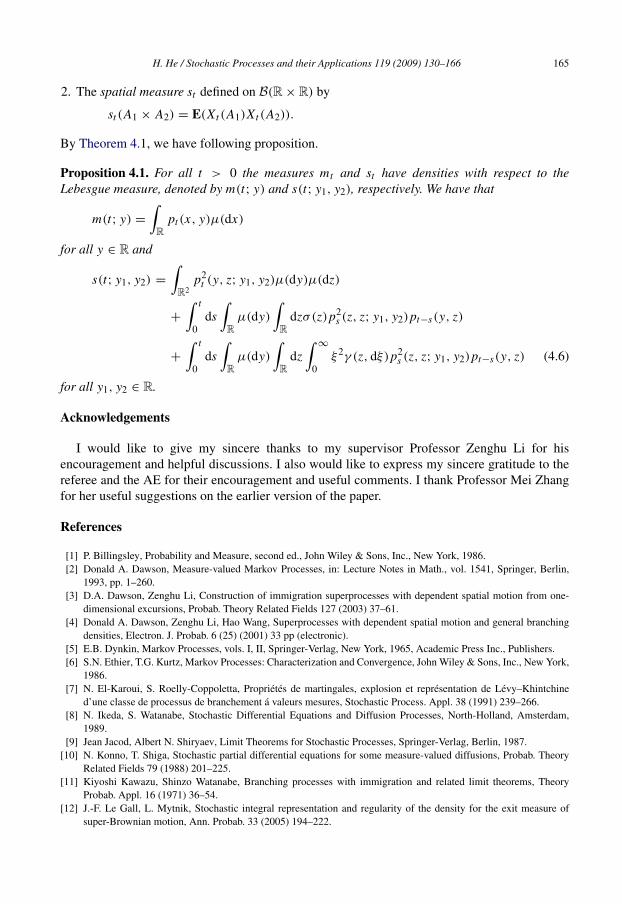
H. He / Stochastic Processes and their Applications 119 (2009) 130–166 165
2. The spatial measure st defined on B(R× R) by
st (A1 × A2) = E(X t (A1)X t (A2)).
By Theorem 4.1, we have following proposition.
Proposition 4.1. For all t > 0 the measures mt and st have densities with respect to theLebesgue measure, denoted by m(t; y) and s(t; y1, y2), respectively. We have that
m(t; y) =∫R
pt (x, y)µ(dx)
for all y ∈ R and
s(t; y1, y2) =
∫R2
p2t (y, z; y1, y2)µ(dy)µ(dz)
+
∫ t
0ds∫Rµ(dy)
∫R
dzσ(z)p2s (z, z; y1, y2)pt−s(y, z)
+
∫ t
0ds∫Rµ(dy)
∫R
dz∫∞
0ξ2γ (z, dξ)p2
s (z, z; y1, y2)pt−s(y, z) (4.6)
for all y1, y2 ∈ R.
Acknowledgements
I would like to give my sincere thanks to my supervisor Professor Zenghu Li for hisencouragement and helpful discussions. I also would like to express my sincere gratitude to thereferee and the AE for their encouragement and useful comments. I thank Professor Mei Zhangfor her useful suggestions on the earlier version of the paper.
References
[1] P. Billingsley, Probability and Measure, second ed., John Wiley & Sons, Inc., New York, 1986.[2] Donald A. Dawson, Measure-valued Markov Processes, in: Lecture Notes in Math., vol. 1541, Springer, Berlin,
1993, pp. 1–260.[3] D.A. Dawson, Zenghu Li, Construction of immigration superprocesses with dependent spatial motion from one-
dimensional excursions, Probab. Theory Related Fields 127 (2003) 37–61.[4] Donald A. Dawson, Zenghu Li, Hao Wang, Superprocesses with dependent spatial motion and general branching
densities, Electron. J. Probab. 6 (25) (2001) 33 pp (electronic).[5] E.B. Dynkin, Markov Processes, vols. I, II, Springer-Verlag, New York, 1965, Academic Press Inc., Publishers.[6] S.N. Ethier, T.G. Kurtz, Markov Processes: Characterization and Convergence, John Wiley & Sons, Inc., New York,
1986.[7] N. El-Karoui, S. Roelly-Coppoletta, Proprietes de martingales, explosion et representation de Levy–Khintchine
d’une classe de processus de branchement a valeurs mesures, Stochastic Process. Appl. 38 (1991) 239–266.[8] N. Ikeda, S. Watanabe, Stochastic Differential Equations and Diffusion Processes, North-Holland, Amsterdam,
1989.[9] Jean Jacod, Albert N. Shiryaev, Limit Theorems for Stochastic Processes, Springer-Verlag, Berlin, 1987.
[10] N. Konno, T. Shiga, Stochastic partial differential equations for some measure-valued diffusions, Probab. TheoryRelated Fields 79 (1988) 201–225.
[11] Kiyoshi Kawazu, Shinzo Watanabe, Branching processes with immigration and related limit theorems, TheoryProbab. Appl. 16 (1971) 36–54.
[12] J.-F. Le Gall, L. Mytnik, Stochastic integral representation and regularity of the density for the exit measure ofsuper-Brownian motion, Ann. Probab. 33 (2005) 194–222.

166 H. He / Stochastic Processes and their Applications 119 (2009) 130–166
[13] Zhi-Ming Ma, Kai-Nan Xiang, Superprocesses of stochastic flows, Ann. Probab. 29 (2001) 317–343.[14] L.C.G. Rogers, D. Williams, Diffusions, Markov Processes, and Martingales, Volume 1: Foundations, second ed.,
Cambridge University Press, 2000.[15] G. Skoulakis, Robert J. Adler, Superprocesses over a stochastic flow, Ann. Appl. Probab. 11 (2001) 488–543.[16] Daniel W. Stroock, Diffusion processes associated with Levy generators, Z. Wahrscheinlichkeitstheorie und Verw.
Gebiete 32 (1975) 209–244.[17] Daniel W. Stroock, S.R.S. Varadhan, Multidimensional Diffusion Processes, Springer-Verlag, Berlin, New York,
1979.[18] H. Wang, State classification for a class of measure-valued branching diffusions in a Brownian medium, Probab.
Theory Related Fields 109 (1997) 39–55.[19] H. Wang, A class of measure-valued branching diffusions in a random medium, Stoch. Anal. Appl. 16 (1998)
753–786.[20] H. Wang, State classification for a class of interacting superprocesses with location dependent branching, Electron.
Comm. Probab. 7 (2002) 157–167 (electronic).