disaster risk reduction in malaysia and …eprints.utar.edu.my/851/1/ci-2013-0907674-1.pdfdisaster...

DISASTER RISK REDUCTION IN MALAYSIA AND EARTHQUAKE

STUDY BASED ON CYCLIC TRIAXIAL TEST

CHIENG TZE SHENG, ALEXANDER

A project report submitted in partial fulfilment of the

requirements for the award of Bachelor of Engineering

(Hons.) Civil Engineering

Faculty of Engineering and Science

Universiti Tunku Abdul Rahman

May 2013

ii

DECLARATION

I hereby declare that this project report is based on my original work except for

citations and quotations which have been duly acknowledged. I also declare that it

has not been previously and concurrently submitted for any other degree or award at

UTAR or other institutions.

Signature :

Name : Chieng Tze Sheng, Alexander

ID No. : 09UEB07674

Date :

iii

APPROVAL FOR SUBMISSION

I certify that this project report entitled “DISASTER RISK REDUCTION IN

MALAYSIA AND EARTHQUAKE STUDY BASED ON CYCLIC TRIAXIAL

TEST” was prepared by CHIENG TZE SHENG, ALEXANDER has met the

required standard for submission in partial fulfilment of the requirements for the

award of Bachelor of Engineering (Hons.) Civil Engineering at Universiti Tunku

Abdul Rahman.

Approved by,

Signature :

Supervisor : Prof. Dr Yasuo Tanaka

Date :

iv

The copyright of this report belongs to the author under the terms of the

copyright Act 1987 as qualified by Intellectual Property Policy of Universiti Tunku

Abdul Rahman. Due acknowledgement shall always be made of the use of any

material contained in, or derived from, this report.

© 2013, Chieng Tze Sheng, Alexander. All right reserved.

v

Specially dedicated to

my beloved grandparents, mother and father

vi

ACKNOWLEDGEMENTS

I would like to thank everyone who had contributed to the successful completion of

this project. I would like to express my gratitude to my research supervisor, Prof. Dr

Yasuo Tanaka for his invaluable advice, guidance and his enormous patience

throughout the development of the research.

In addition, I would also like to express my gratitude to my loving parent and

friends who had helped and given me encouragement since the first day of this

research till the end. Without all these people, this research will not come to a

success.

vii

DISASTER RISK REDUCTION IN MALAYSIA AND EARTHQUAKE

STUDY BASED ON CYCLIC TRIAXIAL TEST

ABSTRACT

Malaysia is tectonically situated in the relatively stable Subdaland. However,

Malaysia can still experience tremors from the earthquakes generated from

neighbouring country. In this research, cyclic triaxial is used to study the dynamic

properties of residual soil. Before running the cyclic loading, the soil is classified

with a few test, namely wet sieve analysis, Atterberg limit test, compaction test, and

in-situ density test. Next, the cyclic triaxial system is also set up by putting together

the loading frame, control panel, triaxial cell, sensors, and programs to acquire data

and control the cyclic loading. Calibrations are carried out on all the sensors required

in this research. This report presents the data obtained from the cyclic triaxial test of

compacted residual soil with a density of 16kN/m3, and the author concluded that the

frequency did not affect greatly the shear modulus and damping ratio. The results of

cyclic triaxial test on compacted residual soil with a density of 15 kN/m3 will be

presented by Boon (2013). On the other hand, the shear modulus decreased with the

increase of stress ratio, whereas damping ratio increased with the stress ratio. Other

than that, the graph of shear modulus vs shear strain and damping ratio vs shear

strain is obtained. Plus, the author also concluded that the Local Deformation

Transducer (LDT) is more reliable than Linear Variable Displacement Transformer

(LVDT).

viii

TABLE OF CONTENTS

DECLARATION ii

APPROVAL FOR SUBMISSION iii

ACKNOWLEDGEMENTS vi

ABSTRACT vii

TABLE OF CONTENTS viii

LIST OF TABLES xi

LIST OF FIGURES xii

LIST OF SYMBOLS / ABBREVIATIONS xv

LIST OF APPENDICES xvii

CHAPTER

1 INTRODUCTION 1

1.1 Background of Study 1

1.2 Aims and Objectives 2

1.3 Layout of Report 2

2 LITERATURE REVIEW 3

2.1 Introduction 3

2.2 Vulnerability and Seismic Activity in Malaysia 3

2.3 Advantages and Disadvantages of Cyclic Triaxial Test 6

2.4 Factors Affecting Dynamic Properties 8

2.5 Sample Preparation by Static Compaction 9

2.6 Dynamic Properties of Residual Soil in Singapore 11

ix

3 METHODOLOGY 12

3.1 Introduction 12

3.2 Soil Sampling 12

3.3 Soil Classification Tests 14

3.3.1 Wet Sieve Analysis 14

3.3.2 Atterberg Limit Test 15

3.3.3 Compaction Test 17

3.3.4 In-Situ Density Test 19

3.4 Set Up of Cyclic Triaxial System 21

3.4.1 Loading Frame 21

3.4.2 Control Panel 22

3.4.3 Triaxial Cell 25

3.4.4 Sensors 26

3.4.4.1 Load Cell 26

3.4.4.2 LVDT 27

3.4.4.3 LDT 28

3.4.5 Data Acquisition with LabVIEW 29

3.4.6 Controlling DP Transducer with LabVIEW 32

3.5 Calibration 35

3.5.1 DP Transducer Calibration 35

3.5.2 Load Cell Calibration 36

3.5.3 Axial Load Calibration 37

3.5.4 LVDT Calibration 38

3.5.5 LDT Calibration 40

3.6 Testing Procedure 42

3.6.1 Test Specimen Preparation 42

3.6.2 Specimen Mounting Procedure 44

3.6.3 Consolidation 46

3.6.4 Cyclic Loading 47

3.7 Data Analysis 48

x

4 RESULTS AND DISCUSSION 54

4.1 Introduction 54

4.2 Dynamic Properties 54

4.3 Discussion 61

4.4 Problems Encountered 75

5 CONCLUSIONS AND RECOMMENDATIONS 78

5.1 Conclusions 78

5.2 Recommendations 78

REFERENCES 80

APPENDICES 82

xi

LIST OF TABLES

TABLE TITLE PAGE

2.1 Frequency and Intensity of Felt Earthquakes

Recorded from 1874 to 2010 (Sherliza et al,

2012) 6

2.2 Summary of Shear Strength Value for all Soil

(Doris and Hafez, 2011) 10

3.1 Wet Sieve Data 14

3.2 Atterberg Limit Test Data (Part 1) 16

3.3 Atterberg Limit Test Data (Part 2) 16

3.4 Compaction Test Data 18

3.5 In-Situ Density Test Data (Part 1) 20



4.1 Shear Modulus 54

4.2 Damping Ratio 56

4.3 Error with Data 61

4.4 Basic Index Properties of JF and BT soils (Tou,

2003) 64

4.5 Experimental Parameters for Soil Specimens

JF1, JF2 and BT (Tou, 2003) 65

4.6 JF2 Converted Result 72

xii

LIST OF FIGURES

FIGURE TITLE PAGE

2.1 Maximum Observed Earthquake Intensity

(MMI Scale) for Peninsular Malaysia from

MMD 4

2.2 Maximum Observed Earthquake Intensity

(MMI Scale) for Sabah and Sarawak from

MMD 5

2.3 Full-Bridge Configuration 8

2.4 X-ray Photo for Dynamic and Static Compacted

Soil 10

3.1 Hammering the Twelve Nails into the Soil 13

3.2 Plastering of the Undisturbed Soil Sample 13

3.3 Graph of percentage of finer vs particle size 15

3.4 Graph of Water Content vs Penetration 17

3.5 Graph of Dry Density vs Moisture Content 18

3.6 Obtaining the Soil Sample 19

3.7 Water is Poured into the Hole 20

3.8 Assembling the Cyclic Triaxial Frame 22

3.9 Cyclic Triaxial System Diagram 23

3.10 Cyclic Triaxial Control Panel 24

3.11 Cyclic Triaxial Cell 25

3.12 Piston Connector 26

3.13 Wire Sealed with Epoxy 27

xiii

3.14 Linear Variable Deformation Transformer 28

3.15 Full Bridge Connection of Local Deformation

Transducer 28

3.16 Block Diagram of Data Acquisition Program 30

3.17 Front Panel of Data Acquisition Program 31

3.18 DAQCard-1200 I/O Connector Pin Assignments

(National Instruments, 1999) 32

3.19 Generate Sine Wave 33

3.20 Cycle Counter 33

3.21 Generate Sine Wave Start Button 34

3.22 Air Pressure Controller Front Panel 34

3.23 Calibration of LVDT 39

3.24 Initial Position of LVDT 39

3.25 Initial Position of LDT 40

3.26 Compacting the Soil 43

3.27 Compacted Soil Sample 43

3.28 Membrane Folded Over the Membrane

Stretcher 44

3.29 Soil Sample with Filter Paper 45

3.30 Attaching the LDT to the Membrane 45

3.31 Consolidation Process 47

3.32 Area of Triangle 52

4.1 Graph of Shear Modulus vs Frequency 57

4.2 Graph of Damping Ratio vs Frequency 57

4.3 Graph of Shear Modulus vs Stress Ratio 58

4.4 Graph of Damping Ratio vs Stress Ratio 58

4.5 Graph of Shear Modulus vs Shear Strain 59

xiv

4.6 Graph of Damping Ratio vs Shear Strain 59

4.7 Graph of Shear Strain vs Frequency 60

4.8 Graph of Stress Ratio vs Axial Strain 62

4.9 Sensitivity of LVDT 63

4.10 Sensitivity of LDT 63

4.11 Graph of Shear Modulus vs Shear Strain for

JF1 at 390 kPa Consolidation Pressure (Tou,

2003) 65



2003) 66


BT at 290 kPa Consolidation Pressure (Tou,

2003) 66

4.14 Graph of Damping Ratio vs Shear Strain for


2003) 67



2003) 67


BT at 290 kPa Consolidation Pressure (Tou,

2003) 68

4.17 Graph of Shear Modulus and Damping Ratio vs

Frequency for JF1 69


Frequency for JF2 70


Frequency for BT 71

4.20 Comparing with JF2 (47 kPa) 74

4.21 Comparing with JF2 (100 kPa) 74

4.22 LDT is Wrapped Up for Painting 76

4.23 Soil Sample Broken into Half 77

xv

LIST OF SYMBOLS / ABBREVIATIONS

a air pressure, kPa

A constant

Aloop area of hysterical loop

Atriangle area of triangle

A0 initial area, m3

A1 new area, m3

D damping ratio

E young modulus, kPa

F(e) function of e

G shear modulus, kPa

G0 initial shear modulus, MPa

G1 new shear modulus, MPa

m mass, kg or g

n constant

s strain

SR1 stress ratio at first point

SR2 stress ratio at second point

v voltage, V

γ shear strain

ε1 axial strain of first point

ε2 axial strain of second point

εa axial strain

σd deviatoric stress, kPa

σc consolidation pressure, kPa

xvi

σc0 initial confining pressure, MPa

σc1 new confining pressure, MPa

σ1 stress of first point, kPa

σ2 stress of second point, kPa

μ poisson ratio

BT Bukit Timah Granite

JF Jurong Formation

LDT local deformation transducer

LVDT linear variable displacement transformer

MMI modified mercalli intensity

MMD Malaysian meteorological department

xvii

LIST OF APPENDICES

APPENDIX TITLE PAGE

A Calibration of Air Pressure Transducer 82

B Calibration of Load Cell Limit 84

C Calibration of Load Cell 85

D Calibration of Air Pressure Transducer with Load

Cell 87

E Calibration of LVDT 89

F Calibration of LDT Initial Position 92

G Calibration of LDT 93

H Test Specimen Data 95

I Consolidation Data 97

CHAPTER 1

1 INTRODUCTION

1.1 Background of Study

Malaysia is located on the Sundaland, which is relatively stable from earthquake.

(Sherliza et. al, 2012). This does not mean that Malaysia is free from earthquake

tremors generated locally and from neighbouring country. The highest recorded

Modified Mercalli Intensity Scale (MMI) in West Malaysia is VI, whereas for East

Malaysia is VII. The scale of VII is able to produce a moderate damage to well-built

ordinary structures and a considerable amount of damage to poorly-built structures.

However, less than one percent of buildings in Malaysia are seismic resistant

(Taksiah Abdul Majid, 2009).

To design any geotechnical engineering problems that involve dynamic

loading of soils and soil-structure interaction systems requires the determination of

two important parameters, the shear modulus and the damping ratio of the soils

(Sitharam, 2004). In this research, these two parameters are obtained from the soil

sampled from Shah Alam, Selangor.

In addition, the data for the dynamic properties of soil in Malaysia is very

rare as there are not many researchers in Malaysia is studying about these dynamic

properties. Therefore, more of these researches should be done in Malaysia to

provide a large database in order to improve the structure and to reduce the disaster

risk in Malaysia.

2

1.2 Aims and Objectives

The aim of this project is to obtain the dynamic properties of the soil obtained from

Alam Impian, Shah Alam, Selangor, with the coordinate of 3°1'36.23"N,

101°30'57.36"E. The specific objectives are set forth:

i. To classify the soil collected from the site.

ii. To set up the cyclic triaxial system.

iii. To obtain the shear modulus and damping ratio of the soil.

iv. To plot a graph of shear modulus vs. shear strain and damping ratio vs.

shear strain.

1.3 Layout of Report

This thesis is divided into five chapters. The first chapter describes about the

background study, aims and objectives, significance of study and the layout of report.

On the other hand, the second chapter deals with the vulnerability and seismic

activity in Malaysia, the advantages and disadvantages of cyclic triaxial test, the

factors affecting dynamic properties, the comparison between dynamic compaction

and static compaction, and the dynamic properties of residual soil in Singapore.

Furthermore, the third chapter explains about the research methodology. This

chapter describes every steps in detail for soil sampling, soil classification, set up of

cyclic triaxial system, calibrations, and the testing of the sample. Next, the fourth

chapter deals with about the results and discussion. This chapter shows and discusses

the dynamic properties obtained from the test and also the problems encountered.

Lastly, the fifth chapter presents the conclusions and the future recommendations for

this research.

CHAPTER 2

2 LITERATURE REVIEW

2.1 Introduction

This chapter presents the vulnerability and seismic activity in Malaysia, the

advantages and disadvantages of cyclic triaxial test, the factors affecting dynamic

properties, the comparison between dynamic compaction and static compaction, and

the dynamic properties of residual soil in Singapore.

2.2 Vulnerability and Seismic Activity in Malaysia

Malaysia is a country that falls under low seismicity group and a seismotectonic

study has been conducted by the Mineals and Geoscience Department of Malaysia

(MGDM) that confirms Malaysia is tectonically situated in the relatively stable

Subdaland (Sherliza et. al, 2012). However, it does not mean that Malaysia is free

from earthquake threat because it lies close to Sumatran faut and Sumatran

Subduction zone. Huge earthquakes that originated from these two active areas did

create considerably ground motion over western part of West Malaysia.

On 4 June 2000, Bengkulu Earthquake occurred in the Sumatran subduction

zone had shook several buildings in Johor Bahru and Klang Valley. Minor cracks in

the building wall was reported in Johor Bahru and the maximum observed intensity

4

in Johor Bahru and Kuala Lumpur was estimated of about VI on Modified Mercalli

Intensity (MMI) scale (Rosaidi, 2001).

Whereas, the Sumatran Fault ruptured at magnitude of about 7.0 on Richter

Scale in the 1995 and about 450km away from Johor. This also has an intensity of VI

on MMI scale. In addition, the 1996 event with magnitude of about 5.4 on Richter

Scale and about 300km from coast of Perak also shook many high-rise buildings in

Penang, Perak, Kuala Lumpur and Selangor. The observed intensity was also VI on

MMI scale (Rosaidi, 2001).

On the other hand, East Malaysia is classified as moderately active in

seismicity. Sabah is the only state that has the most earthquake activities in Malaysia.

The maximum observed intensity in Lahad Datu and Kunak was estimated of about

VII on MMI scale. Other than that, Sarawak also experienced several earthquakes of

local origin. Over the last 35 years, a total of three earthquake occurred in Sarawak

with maximum observed intensity of IV on MM scale. Besides, these two states also

affected by earthquake originated from Southern Philippine, Makassar Strait, Sulu

Sea and Celebes Sea (Rosaidi, 2001).

Based on the information obtained from the Malaysian Meteorological

Department (MMD), the maximum recorded MMI scale from 1875 to 2011 for East

Malaysia is VII, whereas the largest recorded MMI scale from 1909 to 2011 for West

Malaysia is VI. This data is shown in the two figures below.

Figure 2.1: Maximum Observed Earthquake Intensity (MMI Scale) for

Peninsular Malaysia from MMD

5

Figure 2.2: Maximum Observed Earthquake Intensity (MMI Scale) for Sabah

and Sarawak from MMD

According to the MMI scale description, for the scale of VII, which is the

highest recorded MMI scale in Malaysia, it states that there will be a moderate

damage occur to well-built ordinary structures and also considerable amount of

damage in poorly built or badly designed structures. However, less than one percent

of buildings in Malaysia are seismic resistant (Taksiah Abdul Majid, 2009).

On the other hand, the table from Sherliza et al (2012) summarized the

frequency and intensity of felt earthquakes recorded from 1874 to 2010 for every

states in Malaysia is shown below.

6

Table 2.1: Frequency and Intensity of Felt Earthquakes Recorded from 1874 to

2010 (Sherliza et al, 2012)

This shows that Malaysia is quite vulnerable to earthquake. Therefore, more

research should be done in Malaysia to provide a large database of earthquake related

information, which will be useful for the purpose of disaster risk reduction.

2.3 Advantages and Disadvantages of Cyclic Triaxial Test

There are a few advantages and disadvantages of this cyclic triaxial test. In the past

40 years, most of the liquefaction testing of sands, silts, and even low plasticity clays

has been performed using this triaxial equipment. Therefore, there is a large database

of information accumulated throughout these years of testing. This has benefited the

7

engineering community by improving the ability to draw rational conclusions on the

cyclic response of untested materials by comparing responses of other soils within

the database (Jennifer et al, 2007).

The main disadvantage of this triaxial test is that it does not reflect the actual

field conditions. The earthquake motion replicated with this equipment is not

vertically propagating horizontal shear waves, but a cyclic vertical loading. Besides,

the specimens are typically isotropically consolidated, whereas the soil in the field is

usually anisotropically consolidated. In addition, the rotation of the principal stresses

during loading is also different. The direction of the major principal stress in triaxial

test will instantaneously rotate 90º from vertical to horizontal and then back.

However, the major principal stress will rotate smoothly and remain nearly vertical

in the field (Jennifer et al, 2007).

Another problem with the triaxial cyclic test it the occurrence of "necking"

during the extension phase of loading. The term, "necking" defines as the local

decrease in cross-sectional area, which induces significant stress concentrations.

When significant stresses are induced, the experimental stress-strain measurements

will be affected due to the inconsistency of the global volume throughout the

specimen. (Jennifer et al, 2007).

In addition, the cyclic triaxial used in this research is using a sensor called

Local Deformation Transducer (LDT). This sensor is able to measure up to around

10-5

to 10-6

of strain, which is beyond what many other sensors can do, such as the

Linear Variable Displacement Transformer (LVDT). This LDT functions based on

the concept of Wheatstone bridge. A Wheatstone bridge is a network of four resistive

legs. One or more of these legs and the below shows the Full-Bridge configuration.

In this research, the LDT is constructed by using the Full-Bridge configuration,

where four strain gauges are used. The procedure of fabricating this LDT is

explained in Chapter 3.

8

Figure 2.3: Full-Bridge Configuration

2.4 Factors Affecting Dynamic Properties

In order to evaluate the reaction of foundations subjected to vibrations and the

manner of vibrations and its transmission through the soil, the dynamic properties of

the soil must be determined (T.G. Sitharam et al, 2004). There are several factors that

affect the dynamic properties of soil, especially the shear modulus and damping ratio.

Many researches have been conducted in the past by experts around the world and

their conclusions are explained below.

Hardin and Richart (1963) (in Martin, 1990) conclude that the shear modulus

of sand varied with the square root of the isotropic confining pressure. Besides, they

also proved that the void ratio was one of the most significant variables affecting

shear modulus, along with other properties like moisture content, grain

characteristics, and gradation influencing the modulus mainly by how they affect

void ratios.

On the other hand, Hardin and Black (1966) (in Martin, 1990) concludes that

the stress modulus of normally consolidated clay also proportional to the square root

of the confining pressure. Plus, they also concluded that the function relationship for

shear modulus would include many factors such as effective octahedral normal stress,

void ratio, ambient stress and vibration history, degree of saturation, octahedral shear

stress, grain characteristics, grain shape, grain size, grading, mineralogy, amplitude

of vibration, frequency of vibration, secondary effects that are a function of time, soil

structure, and temperature, including freezing.

9

In addition, Hardin and Black (in Martin, 1990) also stated that the mean

effective stress, void ratio and strain amplitude are the most important factors

affecting shear modulus. The degree of saturation and overconsolidation ratio were

also important for cohesive soils, but appeared less important for sands.

The damping values are affected by the same factors that influence the shear

modulus. The difference is that damping is affected oppositely of shear modulus. In

other words, as the shear modulus increases, the damping will decrease and vice

versa. In an ideal condition, the maximum damping value can be archived when

shear modulus is equal to zero (Pieter, 1992).

2.5 Sample Preparation by Static Compaction

In this research, static compaction is used to prepare the soil sample for testing. The

difference between statically or dynamically compacting sample affects the test

results on soil properties. A static compaction will produce a soil sample that is

stiffer, stronger and less plastic compared to specimen produced from dynamic

compaction (Doris and Hafez, 2011).

Besides, the static compaction also gives a higher shear strength value. This

is shown in the table below by Doris and Hafez.

10

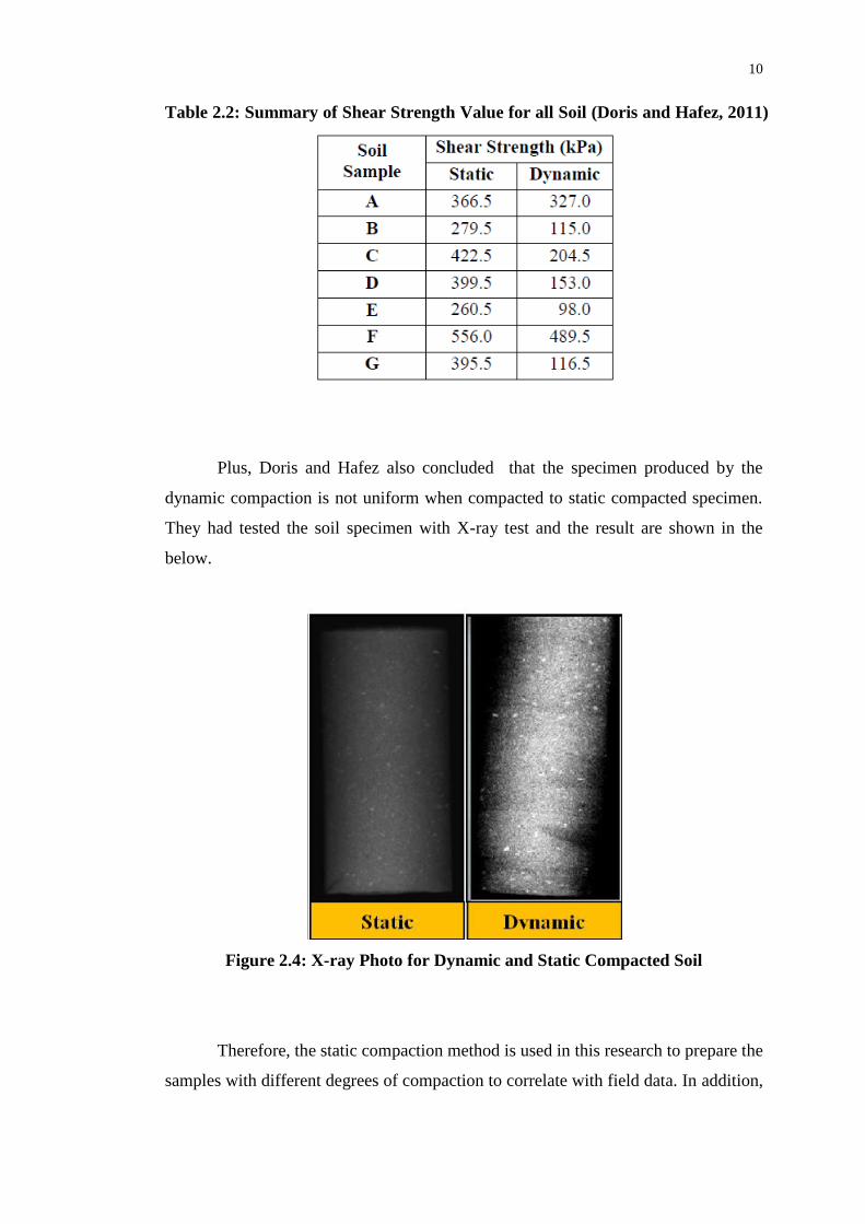
Table 2.2: Summary of Shear Strength Value for all Soil (Doris and Hafez, 2011)

Plus, Doris and Hafez also concluded that the specimen produced by the

dynamic compaction is not uniform when compacted to static compacted specimen.

They had tested the soil specimen with X-ray test and the result are shown in the

below.

Figure 2.4: X-ray Photo for Dynamic and Static Compacted Soil

Therefore, the static compaction method is used in this research to prepare the

samples with different degrees of compaction to correlate with field data. In addition,

11

this method is also faster, easier and simpler to be carried out in the laboratory

compared to dynamic compaction method.

2.6 Dynamic Properties of Residual Soil in Singapore

In Singapore, the dynamic properties of residual soil have been studied by cyclic

triaxial test. Tou (2003) has studied the dynamic properties of two different

Singapore soils and they are the Jurong Formation residual soils and Bukit Timah

Granite residual soil.

Tou (2003) shows that the shear modulus of the soil decreases with the

increase in shear strain and the damping ratio increasing with the increase of shear

strain. Additionally, he shows that the shear modulus and damping ratio at certain

shear strain level increase as the frequency increases. This is more obvious at small

shear strain levels like 0.01 %, 0.02 % and 0.03 % (Tou, 2003).

Plus, by comparing the normalized shear modulus and damping ratio for

saturated sand and clays show that the dynamic properties of the test specimen fall in

the average range of saturated sand, whereas the damping ratio of the specimen is

higher compared to those of saturated sand (Tou, 2003).

In addition, Tou (2003) also compared the normalized shear modulus of the

soil sample with those of Piedmond residual soils. It does not show a great variation

with the average trend of Piedmond residual soils. However, the damping ratio of the

residual soil specimen shows a higher value in comparison (Tou, 2003).

Besides, the shear moduli determined 'locally' by using a pair of Local

Deformation Transducer (LDT) generally show higher values compared with the

shear modulus determined 'externally' using the Linear Variable Displacement

Transformer (LVDT) especially at small shear strain levels like 0.01 %, 0.02 % and

0.03 %. This shows the importance of local strain measurement in cyclic triaxial test

(Tou, 2003). The results by Tou (2003) are further discussed in Chapter 4.

CHAPTER 3

3 METHODOLOGY

3.1 Introduction

This chapter explains the methodology of every activities done throughout this whole

research such as the soil sampling method, soil classification, set up of cyclic triaxial

system, calibration of sensors and air pressure, and the cyclic triaxial testing

procedure.

3.2 Soil Sampling

Firstly, a soil testing company, Sealand Teknikal Sdn Bhd, is contacted by the

author's research supervisor. Then a site in Shah Alam, Selangor, with the coordinate

3°1'36.23"N, 101°30'57.36"E is recommended by the soil testing company. After the

site visitation by the author's research supervisor, the location is decided and

preparation for soil sampling is started.

Two types of soil are obtained from the site, namely the undisturbed and

disturbed residual soils. For collecting undisturbed sample, the following procedures

are used. First, the top layer of the soil being removed and flattened to place a

wooden plate for soil nail sampling. By hammering the 23 cm long nails along the

plate into the ground, a block of undisturbed soil is securely held in position so that

13

this soil block can be excavated from the rest of the soil. These nails also act as a

support for the soil once the soil is taken out.

Figure 3.1: Hammering the Twelve Nails into the Soil

Once the soil sample is taken out, it is then carefully overturned and a layer

of plaster is pasted on the whole soil sample. Thus the soil was kept undisturbed and

prevented from the loss of moisture. Then the soil is transported to laboratory by

being wrapped by air bubble sheet.

Figure 3.2: Plastering of the Undisturbed Soil Sample

14

Additionally, disturbed residual soil was collected by simply excavating the

ground and transported to laboratory in a bag. Disturbed soil is dried under the sun

and then physical and compaction tests were carried out by using air-dried sample.

For this current Final Year Project research, only the disturbed samples are used and

the undisturbed samples are kept for the future research.

3.3 Soil Classification Tests

This section presents the results of the wet sieve analysis, Atterberg limits test using

cone penetrometer and compaction test based on the procedure from BS 1377.

3.3.1 Wet Sieve Analysis

The table below shows the data obtained from wet sieve analysis and a graph of

percentage of finer vs particle size is plotted and shown as well.

Table 3.1: Wet Sieve Data

Mesh

Aperture

(mm)

Mass

of

Tray

(g)

Mass

of

Tray

with

Soil

(g)

Mass of

Soil

Retained

(g)

Mass of

Soil

Retained

(%)

Cumulative

of coarser

(%)

Cumulative

of finer

(%)

2.000 36.3 36.8 0.5 0.250 0.250 99.750

1.180 53.7 61.2 7.5 3.750 4.000 96.000

0.600 34.3 55.9 21.6 10.800 14.800 85.200

0.425 34.3 56.4 22.1 11.050 25.850 74.150

0.300 34.7 49.9 15.2 7.600 33.450 66.550

0.212 34 53.4 19.4 9.700 43.150 56.850

0.150 34.3 68.2 33.9 16.950 60.100 39.900

0.063 36.2 66.7 30.5 15.250 75.350 24.650

receiver 49.3 24.650 100.000 0.000

Total 200 100.000

15

Figure 3.3: Graph of percentage of finer vs particle size

From the graph above, less than 35 % of the material is finer than 0.063 mm

and more than 50 % of coarse material is of sand size (finer than 2mm). Based on BS

5930.81, this soil is categorised under sand.

3.3.2 Atterberg Limit Test

The table below shows the data obtained from the Atterberg Limit Test with cone

penetrometer. The label LL is for liquid limit test, whereas label with PL is for

plastic limit test.

0.000

20.000

40.000

60.000

80.000

100.000

120.000

0.010 0.100 1.000 10.000

%Fi

ne

r

Particle size (mm)

Graph of Percentage Finer against Particle Size

16

Table 3.2: Atterberg Limit Test Data (Part 1)

Label Mass of Tray (g)

Mass of

Tray

with

Moisture

soil (g)

Mass of

Moisture

soil (g)

Penetration

value

(mm)

LL1 34.1 36.6 2.5 16.8

LL2 33.7 39.3 5.6 17

LL3 33.8 40.7 6.9 19.8

LL4 34.4 40.4 6 22.5

LL5 35.5 45.5 10 23.7

PL 33.9 36.1 2.2 -

Table 3.3: Atterberg Limit Test Data (Part 2)

Label

Mass of

Tray

with

Dried

soil (g)

Mass of

dried

soil (g)

Mass

Moisture

Content

(g)

Moisture

content

(%)

LL1 35.7 1.6 0.9 56.25

LL2 37.3 3.6 2 55.56

LL3 38.1 4.3 2.6 60.47

LL4 38 3.6 2.4 66.67

LL5 41.4 5.9 4.1 69.49

PL 35.6 1.7 0.5 29.41

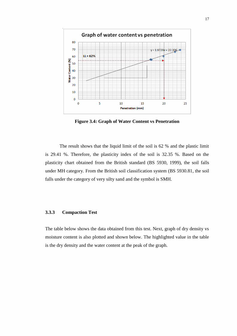
In addition, graph of water content vs penetration is plotted and the liquid

limit is obtained. This graph is shown in the below.

17

Figure 3.4: Graph of Water Content vs Penetration

The result shows that the liquid limit of the soil is 62 % and the plastic limit

is 29.41 %. Therefore, the plasticity index of the soil is 32.35 %. Based on the

plasticity chart obtained from the British standard (BS 5930, 1999), the soil falls

under MH category. From the British soil classification system (BS 5930.81, the soil

falls under the category of very silty sand and the symbol is SMH.

3.3.3 Compaction Test

The table below shows the data obtained from this test. Next, graph of dry density vs

moisture content is also plotted and shown below. The highlighted value in the table

is the dry density and the water content at the peak of the graph.

18

Table 3.4: Compaction Test Data

Figure 3.5: Graph of Dry Density vs Moisture Content

In conclusion, the maximum dry density with the value of 1.76 Mg/m3 falls

on the water content of 14.66 %.

1.50

1.55

1.60

1.65

1.70

1.75

1.80

10.00 12.00 14.00 16.00 18.00 20.00

Dry

de

nsi

ty ρ

d (

Mg/

m3

)

Moisture content

Graph of Dry Density vs Moisture Content

19

3.3.4 In-Situ Density Test

In-Situ Density Test is carried out in the site itself to determine the density of the soil

at the site. This can be done by first flattening the soil surface. Then, a square

cardboard with a hole in the middle is placed on it and held firmly. The hole must be

big enough for the soil sampler to pass through. The purpose of this cardboard is to

act as a guide and to prevent the soil that is going to be dug out to be mixed up with

the surrounding soil. After that, soil is dug out from the hole carefully with a small

spade and soil sampler, making sure that the all soil that is dug out from the hole is

collected in a bag and labelled.

Figure 3.6: Obtaining the Soil Sample

Next, a plastic bag is placed in the hole and water is poured in until it reached

the surface. Hand is used to push the plastic to the soil surface in the hole to make

sure that the water in the plastic bag covered all the void in the hole. After that, the

plastic bag is removed from the hole, tied properly and labelled. The above test is

repeated few more times on two different location, namely Site A and Site B.

20

Figure 3.7: Water is Poured into the Hole

The volume of water in the plastic bag is measured and recorded immediately

after the plastic bag is taken out from the hole, whereas the soil samples collected

are brought back to the laboratory to be weighted and dried. Then, the moisture

content and density is calculated. The data obtained from this test is shown below.

Table 3.5: In-Situ Density Test Data (Part 1)

Sample Volume

(ml) Mass of Tray

(g) Mass of Tray with Undried

Soil (g) Mass of Tray with Dried

Soil (g)

B2 1308 680.8 2956.3 2589.5

B3 1149 677.4 2827.4 2444

A1 1330 685.1 3235.7 2838.7

A2 1465 693 3482.9 3007.3


Sample Volume

(m3) Mass of Dry

Soil (kg) Density (kg/m3)

B2 0.001308 1.909 1459.48

B3 0.001149 1.767 1537.86

A1 0.00133 2.154 1619.56

A2 0.001465 2.314 1579.52

21


Sample

Water Content

(kg) Water Content

(%)

B2 0.3668 0.192

B3 0.3834 0.217

A1 0.397 0.184

A2 0.4756 0.206

From the result obtained, the density of the soil in Site A is approximately 16

kN/m3 and B is around 15 kN/m

3. On the other hand, the water content of both site is

approximately 20%.

3.4 Set Up of Cyclic Triaxial System

In this section, all the procedures involving the set up of the cyclic triaxial system

will be explained. This involves the set up of the loading frame, control panel,

triaxial cell, sensors, data acquisition program and air pressure controller program.

3.4.1 Loading Frame

The loading frame of this cyclic triaxial system is fabricated in the university

laboratory by a laboratory officer, Mr. Hwong. It consists of four long columns with

a top and bottom plate. All the parts are cleaned and painted with silver paint to

avoid corrosion before putting them together. To make sure that the top and bottom

plates are levelled, washers are placed on the columns to adjust the height of the

plate with the help of spirit level. Once everything is set, all the nuts are tighten with

a spanner. After that, the air pressure cylinder is placed on top of the top plate and

locked in the position.

22

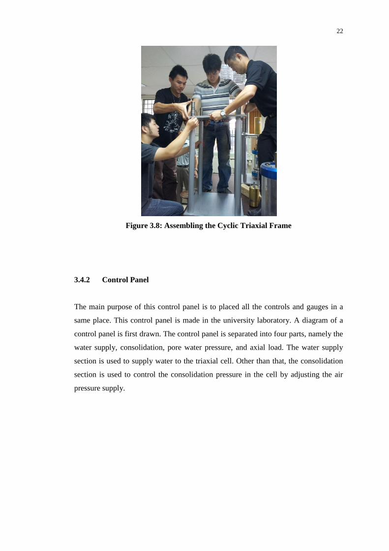
Figure 3.8: Assembling the Cyclic Triaxial Frame

3.4.2 Control Panel

The main purpose of this control panel is to placed all the controls and gauges in a

same place. This control panel is made in the university laboratory. A diagram of a

control panel is first drawn. The control panel is separated into four parts, namely the

water supply, consolidation, pore water pressure, and axial load. The water supply

section is used to supply water to the triaxial cell. Other than that, the consolidation

section is used to control the consolidation pressure in the cell by adjusting the air

pressure supply.

23

Figure 3.9: Cyclic Triaxial System Diagram

In addition, the pore water pressure section is used to supply the pressurised

de-aired water to the soil sample in the cell. This can be done by supplying the air

pressure into the tank filled with de-aired water before directing the water into the

cell. On the other hand, there is also a glass tube with a ruler beside in this section.

This is to observe the consolidation duration to make sure that the sample is

completely consolidated by allowing the pore water to flow out into the glass tube.

The axial load section consists of both the manual air pressure transducer and

the differential pressure transducer. This is to supply air pressure to the top and

bottom of the air pressure cylinder. This will then apply load to the test specimen. A

manual air pressure transducer is used at to supply the air pressure to the bottom of

the cylinder manually, whereas the top cylinder is supplied by the differential

pressure transducer that is controlled by an air pressure control program to generate a

cyclic loading.

A PVC board is chosen to be the board of the control panel and L-shaped

steel is chosen to be make frame. All the parts required like the air pressure

transducer, air pressure gauge, differential pressure transducer, valves, connectors,

24

glass tube, and ruler are placed and marked on the board. Next, the board and steel

are cut into a proper length and holes are drilled on the board. After that, the board

and frame are put together with nuts and bolts before securing all the parts on the

board with locking straps. Locking straps are used for easy removal and assemble if

the parts needed to be changed.

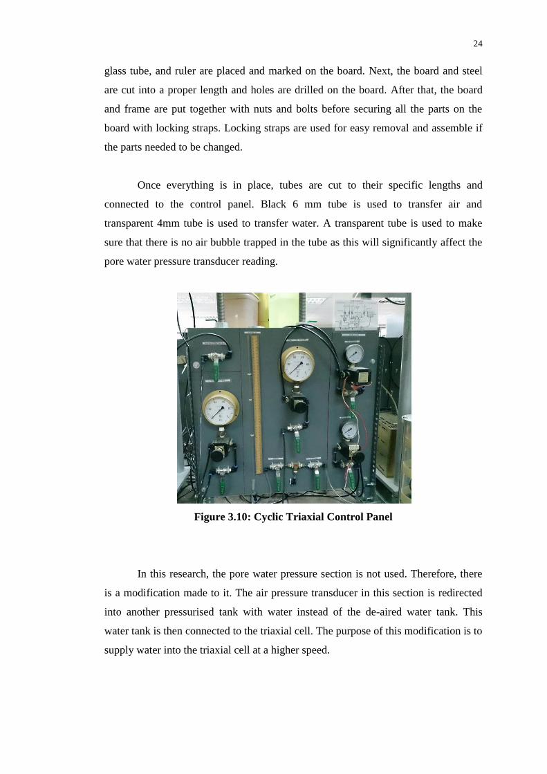
Once everything is in place, tubes are cut to their specific lengths and

connected to the control panel. Black 6 mm tube is used to transfer air and

transparent 4mm tube is used to transfer water. A transparent tube is used to make

sure that there is no air bubble trapped in the tube as this will significantly affect the

pore water pressure transducer reading.

Figure 3.10: Cyclic Triaxial Control Panel

In this research, the pore water pressure section is not used. Therefore, there

is a modification made to it. The air pressure transducer in this section is redirected

into another pressurised tank with water instead of the de-aired water tank. This

water tank is then connected to the triaxial cell. The purpose of this modification is to

supply water into the triaxial cell at a higher speed.

25

3.4.3 Triaxial Cell

This triaxial cell is imported from Kobe University in Japan by the author's research

supervisor. A slight modification is made to it to suits our test by changing the valves

and connectors. Some of the additional holes are sealed up to prevent any leakage.

Tubes are connected to this triaxial cell after all the parts are assembled.

Figure 3.11: Cyclic Triaxial Cell

A special connector is fabricated to connect the triaxial cell piston and the

loading piston of the air pressure cylinder. This connector is made to be adjustable on

both ends and a nut is used to tighten it.

26

Figure 3.12: Piston Connector

3.4.4 Sensors

There is a total of three sensors used in this triaxial system. They are the Load Cell,

Linear Variable Differential Transformer (LVDT), and Local Deformation

Transducer (LDT). All these three sensors are explained in this section.

3.4.4.1 Load Cell

A load cell is a transducer used to measure the load in terms of millivolt. This can be

done because there are four strain gauges inside the load cell to measure the strain as

an electrical signal by changing the effective electrical resistance of the wire. All the

strain gauges are arranged in the Wheatstone bridge configuration. The Wheatstone

bridge is explained in Chapter 2. The calibration of this sensor is explained in

Chapter 3.5.2.

Since the reading of load cell is in the unit of millivolt, amplifier is needed to

boost up the voltage to a readable number. This Load Cell is connected to the

27

channel 1 of the amplifier. The offset and amplification of the load cell is then

adjusted carefully to the best adjustment for this research.

This load cell is placed in the triaxial cell, at the bottom of the piston. The

cable is put through a hole on the triaxial cell and sealed properly with epoxy to

avoid leakage when pressurising the tank.

Figure 3.13: Wire Sealed with Epoxy

3.4.4.2 LVDT

LVDT stands for Linear Variable Deformation Transformer. This sensor is used to

measure the axial deformation of the sample. The reading of this LVDT is also in the

unit of millivolt. Therefore, this LVDT is connected to the channel 4 of the same

amplifier used by the Load Cell. The offset and amplification of this LVDT is also

adjusted carefully to the best adjustment for this research. This sensor is calibrated

and the procedure is explained in Chapter 3.5.4. After calibration, this LVDT is

attached to the top of the frame with a magnetic indicator base.

28

Figure 3.14: Linear Variable Deformation Transformer

3.4.4.3 LDT

LDT stands for Local Deformation Transducer. It is used to measure the deformation

of the sample up to 10-5

strain. This LDT is made in the university laboratory. To

make this sensor, four strain gauges are glued permanently to the side of a bronze

strip with two strain gauge on each side. These strain gauges are then covered with a

layer of flexible glue to protect them from water. The configuration of these strain

gauges is using the full Wheatstone bridge.

Figure 3.15: Full Bridge Connection of Local Deformation Transducer

29

Once all the wires are connected, they are sealed with a thin layer of glue for

water proofing. After the glue is dried, this sensor is then tested and calibrated. The

calibration procedure is explained in Chapter 3.5.5.This sensor is then attached to the

side of the soil sample before testing with two clips glued to the membrane.

The voltage received from this LDT is in mV. Therefore, an amplifier is

needed as well. Since this transducer is extremely sensitive, a better amplifier is used.

The amplifier is then adjusted to the best amplification the author can obtain before

doing any calibration. The calibration of this sensor will be explained in Chapter

3.5.5.

3.4.5 Data Acquisition with LabVIEW

LabVIEW is a graphical programming software that uses to create applications to

communicate with hardware such as data acquisition device. This software enable

user to create a user interface to operate the specific instruments. LabVIEW

programs are called virtual instruments, also known as VIs.

In this research, LabVIEW is required to acquire data from the sensors

because that the cyclic loading is continuous and the data acquisition speed must be

fast enough to produce a better result. This precise and fast data acquisition process

is beyond what human can do manually. Therefore, LabVIEW is needed for this

purpose. The hardware used to acquire data is called USB-6210. This device requires

LabVIEW 2009 to run.

A program named Data Acquisition is created with LabVIEW by the author.

The author used the function of While Loop, For Loop, Time Delay, DAQmx Read

(Analog 1D Wfm NChan 1Samp), Split Signals, Waveform Chart, Convert from

Dynamic Data, Property Node, Write to Measurement File, Divide, Multiply, and

30

Add Array Elements are used. The arrangement of all these functions in Block

Diagram is shown in the figures below.

Figure 3.16: Block Diagram of Data Acquisition Program

31

In addition, the Front Panel is the place where all the controls are shown. This

Front Panel is used by user to control this program while using it. The Front Panel is

shown in the figures below.

Figure 3.17: Front Panel of Data Acquisition Program

This program is able to acquire the data at the speed of 0.03 seconds per

sample. Since there are some noises generated by some of the electronic devices and

some external factors, this program also has a function to average the data acquired

by simply changing the number of data to be averaged. By default, the number of

data to be averaged is 5. All the data will be stored in the computer in the file typed

32

by the user. Channel 17 & 18 is set by the author for Load Cell and Channel 19 & 20

is for LVDT, whereas Channel 21 & 22 is for LDT. Channel 17, 19 and 21 are the

positive connection, whereas Channel 18, 20 and 22 are the negative connections.

The file saved is in the format of tdms. An Microsoft Excel plugin called

tdm_excel_add-in_2012.exe is needed to be installed in the computer in order to read

this file with Microsoft Excel. This plugin is included in the CD attached to this

report. The result will be shown in sheet two instead of the first sheet in Microsoft

Excel.

3.4.6 Controlling DP Transducer with LabVIEW

A DP Transducer is also called a Differential Pressure Transducer. This transducer is

used to control the air pressure supply to the air pressure cylinder. LabVIEW is

required to generate a sine wave to the DP Transducer in order to produce a smooth

cyclic loading. DAQCard-1200 device is used for this purpose. This device can only

runs in LabVIEW 6.1 on Windows XP. The connector pin of this device is shown

below.

Figure 3.18: DAQCard-1200 I/O Connector Pin Assignments (National

Instruments, 1999)

33

The channels the author used are Channel 10 and Channel 11. Channel 10 is

the positive connection, whereas the Channel 11 is the negative connection.

A program is created by the author that named Air Pressure Controller. This

program uses the function of While Loop, For Loop, Case Structure, Sine, To Double

Precision Float, Waveform Chart, AO Update Channel, Wait Until Next ms Multiple,

Wait (ms), Property Node, Not, Divide, Multiply, Add and Equal for this program.

The arrangement in the Block Diagram is shown in the figures below.

Figure 3.19: Generate Sine Wave

Figure 3.20: Cycle Counter

34

Figure 3.21: Generate Sine Wave Start Button

The Front Panel will the one with all the controls will appear. All these

controls are used to control the DP Transducer. This Front Panel is shown in the

below.

Figure 3.22: Air Pressure Controller Front Panel

35

3.5 Calibration

The purpose of calibration is to enable us to convert the voltage received from the

sensors to the unit that the author wanted, such as kilogram, bar and millimetre. In

this section, the calibration of Differential Pressure Transducer, Load Cell, axial load,

Linear Variable Deformation Transformer (LVDT), and Local Deformation

Transducer (LDT) is explained in this section of this chapter.

3.5.1 DP Transducer Calibration

This DP Transducer, also known as Differential Pressure Transducer, is calibrated by

connecting to the DAQCard-1200 that is plugged in to the laptop. Data Acquisition

program is used to instruct the DAQCard-1200 to emit voltage to the Differential

Pressure Transducer.

Voltage is increased slowly until the air pressure gauge showed or 1 bar.

Then the voltage value is recorded. After that, the voltage is increased again until the

gauge showed 1.5 bar and the voltage is recorded. This step is repeated a few times

at the interval of 0.5 bar until it reached 5 bar. Next, the voltage is reduced at the

interval of 0.5 bar until it reached 1 bar again. Once all the data is collected, a graph

of Voltage Supply vs Air Pressure is plotted and the gradient of the graph is obtained.

The calibration data is shown in Appendix A.

After calibration, the relationship of voltage supply and air pressure is shown

in the equation below:

(3.1)

where

v = voltage supply, V

a = air pressure, bar

36

3.5.2 Load Cell Calibration

Before calibrating the Load Cell, the limit of this Load Cell should be found first.

This can be done by first placing the triaxial cell on the floor with the Load Cell

attached to the bottom of the piston. A steel cylinder is placed at the place where the

soil sample will be placed to act as a support so that the piston will not go all the way

down. A few steel plates are weighted on a weighing scale and recorded down. Then

the Load Cell is connected to a data logger and the data logger is set to Simple

Measure to measure the strain of the Load Cell.

The initial strain is recorded before placing any load on the piston. Next, the

first load is placed on the piston and the mass of the load and the strain shown in the

data logger is recorded. This step is repeated a few more times until the mass reached

around 15 kg. Then, the steel plate is reduced one by one and the data is recorded for

every removal of the steel plate. After that, a graph of mass vs strain is plotted and

the equation is obtained from the graph. This equation is shown below:

(3.2)

where

m = mass, kg

s = strain, µε

Since the maximum strain it can go is 3000 µε, this value is substituted into

equation 3.2 and obtained the maximum mass, which is 497.72 kg. The data for this

calibration is shown in Appendix B.

After knowing the Load Cell limit, the Load Cell can be calibrated by

connecting the Load Cell to an amplifier. The amplifier is then connected to the

USB-6210 device. After that, the USB-6210 device is plugged in to the laptop. Data

Acquisition program is used to acquire the reading of the Load Cell in the unit of

millivolt.

37

The initial reading of the voltage emitted by the Load Cell is recorded. Then,

the first steel plate is placed on the piston. After that, the mass of the steel plate and

the voltage shown in the Data Acquisition program is recorded. This step is repeated

a few more times with more load placed on the piston until it reached around 80 kg.

Then the step is repeated again by reducing the steel plate one by one. Once the data

is collected, a graph of voltage vs mass is plotted and the gradient is obtained from

the formula of the graph. This calibration data is shown in Appendix C. With the use

of the gradient obtained from the graph, the relationship of voltage and mass is

shown below:

(3.3)

where

v = voltage received from Load Cell, V

m = mass, g

3.5.3 Axial Load Calibration

In order to obtain the relationship of the air pressure supplied to the air pressure

cylinder and the voltage received from the Load Cell, another calibration is done by

first placing the triaxial cell on the triaxial frame and connected the piston of the cell

to the piston of the air pressure cylinder. A steel cylinder is placed in the location

where the soil sample supposed to be placed to act as a support. Then, all the

necessary devices and parts are connected. Next, the voltage emitted by the

DAQCard is increased to increase the air pressure at the interval of 0.5 bar until it

reached 2.5 bar. At each interval, the air pressure and the voltage from the Load Cell

is recorded. This step is repeated again with the decrease of the air pressure at the

same interval.

After obtaining the data, all the voltage obtained from the Load Cell is

converted to mass in gram by using equation 3.3. Then the unit is changed from gram

38

to kilogram by dividing by another one thousand. A graph of mass of load vs air

pressure is plotted and the gradient is obtained. This calibration data is shown in

Appendix D and the relationship of air pressure and mass is shown below:

(3.4)

where

m = mass, kg

a = air pressure, bar

However, the relationship of voltage supplied by DAQCard-1200 and the

load applied to the soil sample must be found. With this relationship, the load can be

controlled by the DAQCard-1200 by simply converting the voltage to kilogram or

vice versa. This relationship can be found by combining equation 3.1 and 3.4 to form

a new equation below:

(3.5)

where

v = voltage supplied by DAQCard-1200, V

m = mass of load acting on soil sample, kg

3.5.4 LVDT Calibration

The Linear Variable Deformation Transducer is calibrated by using a soil sample

extruder. This can be done by clamping the LVDT to one end of the extruder and a

dail gauge is clamped on the other end. By rotating the handle of the extruder, the

metal bar will move horizontally. This will eventually push or release the LVDT and

the dail gauge on the other end will be affected as well. This set up is shown in the

below.

39

Figure 3.23: Calibration of LVDT

The LVDT is connected to the amplifier and the amplifier is connected to the

USB-6210 device that is plugged to the laptop. Once everything is set up, the LVDT

is pushed in until it reached the third line from the tip of the LVDT as shown in the

below. This is to set the initial position of the LVDT. After that, the initial voltage

and the dail gauge reading is recorded.

Figure 3.24: Initial Position of LVDT

Next, the extruder is rotated anti-clockwise slowly until the dial gauge

reading increase by 25 division or 0.25 mm. Then, the voltage reading and the dail

gauge reading is recorded. This step is repeated at the interval of 25 division until

600 division or 6 mm. After that, the extruder is rotated clockwise and the procedure

is repeated again. A graph of voltage vs dail gauge reading is plotted and the data is

40

shown in Appendix E. From the gradient of the graph plotted, the relationship

between voltage and deformation is shown below:

(3.6)

where

v = voltage received from LVDT, V

d = deformation or displacement, 0.01 mm

3.5.5 LDT Calibration

The Local Deformation Transducer is calibrated by using the same extruder used to

calibrate the LVDT. A dial gauge is clamped to once end of the extruder, whereas the

other end is used to place the LDT. A piece of cardboard with a small cut in the

middle is taped on the extruder to hold the LDT by slotting the LDT into the cut. The

set up is shown in the below.

Figure 3.25: Initial Position of LDT

41

Firstly, the initial position of the LDT is set by connecting the LDT to a data

logger that is set to Simple Measure to measure the strain. The initial strain and the

dial gauge reading is recorded. After that, the extruder is rotated anti-clockwise to

compress the LDT for every 15 division of the dial gauge reading until 135 division

or 1.35 mm. For each interval, the reading of the dial gauge and strain from the data

logger is recorded. A graph of strain vs deformation is plotted. This data is shown in

Appendix F.

The graph plotted is in the form of a curve instead of a linear line. This shows

that the response of this LDT will reduce as the deformation go higher. Therefore,

the initial position is set to only 1 mm. The equation of the graph is shown below:

(3.7)

where

s = strain, µε

d = deformation, 0.01mm

From the equation above, the strain of the initial position, which is 1 mm

deformation is calculated to be 2218 µε. To calibrate the LDT, it is first set to this

initial position by connecting it to data logger and deform until it reached 2218 µε.

After that, the LDT is connected to the amplifier and the amplifier is connected to the

laptop with the Data Acquisition program.

The extruder is then rotated at the interval of 5 division from the dial gauge

reading until it reached 150 division or 1.50 mm. At every interval, the dial gauge

reading and the voltage is recorded. The test is repeated from the other direction. All

the data obtained is shown in Appendix G. A graph of strain vs voltage is plotted

and the equation is shown below:

(3.8)

where

d = deformation of LDT, 0.01 mm

42

v = voltage received from LDT, V

3.6 Testing Procedure

In this section, the procedure to perform a test on the soil specimen with the cyclic

triaxial system is explained. This includes the test specimen preparation, the

mounting of the specimen, the consolidation procedure, and the cyclic loading

process.

3.6.1 Test Specimen Preparation

First, the mould is then cleaned and coated with a layer of oil to allow the sample to

be removed from the mould easily. Then mould is clamped with G-clamps. Specially

made wood blocks should be placed in between the G-clamps and the mould to

protect the mould from damaging and also to prevent sliding. This mould is then

placed under the Hydraulic Press Machine with a steel plate at the bottom.

To prepare a specimen, the amount of soil and water is calculated based on

the density of 16 kN/m3 and water content of 20%. This calculation is in Appendix H.

Then, they are mixed together with the water poured in slowly until they are evenly

mixed. This has to be done in a place without any wind to prevent excessive loss of

water from the soil.

After mixing, the soil is separated into four parts. A custom made piston is

measured and marked to four evenly distributed layer. One part of the soil is then

placed into the mould first and the custom made piston is placed into the mould.

Then the compaction process is started until it reached the first marked line. After

that, the piston is removed and the surface of the compacted soil is scratched to give

a better bonding with the next layer. This step is repeated three more times for the

next three layer.

43

Figure 3.26: Compacting the Soil

After compaction, the mould is removed carefully and the dimension of the

sample is measured with a calliper. Plus, the weight of the sample is also taken. This

soil sample is then wrapped up with plastic sheet to prevent any loss of water content

while preparing the other necessary things for testing.

Figure 3.27: Compacted Soil Sample

44

3.6.2 Specimen Mounting Procedure

First, a clean membrane is placed into the membrane stretcher. Then, the membrane

is folded over at the top and bottom of the membrane stretcher. After that, suction is

introduced to the tube of the membrane stretcher to expand the membrane in the

membrane stretcher. Once the membrane is fully expanded inside, the tube is clipped

to maintain the pressure inside the membrane stretcher.

Figure 3.28: Membrane Folded Over the Membrane Stretcher

After that, the soil sample is placed inside the membrane and the clip on the

tube of the membrane stretcher is removed to allow the membrane to wrap around

the soil. Then, the soil sample is removed from the membrane stretcher along with

the membrane. Next, the top and bottom of the excess membrane is folded over,

exposing the top and bottom surface of the soil.

Filter paper is then placed on the top and bottom surface of the soil before

placing it to the triaxial cell. Silicone grease is applied on around the side of the

loading cap and the bottom cap. Rubber bands are placed at the top of the loading

cap. Then, the membrane is folded over the loading cap and bottom cap before

lowering the rubber bands to the loading cap and bottom cap to seal the membrane.

45

Figure 3.29: Soil Sample with Filter Paper

After that, the LDT cable is connected to the amplifier, USB-6210 and laptop.

The bottom LDT clip is glued to the side of the membrane with a fast drying glue.

Then, the Data Acquisition program is started. Once the program is receiving signal

from the LDT, the LDT is placed on the glued bottom clip and adjusted to around -6

to -7 V, which is the 1 mm initial position of the LDT, by using a tweezer to grip on

the top clip that is placed on the top of the LDT. Glue is applied immediately after

the LDT reading is around -6 to -7 V. The tweezer is removed after the glue is dried.

Figure 3.30: Attaching the LDT to the Membrane

46

Next, the LDT cable is detached from the triaxial cell. Grease is applied on

the top and bottom O-ring before placing the triaxial cell cover and locking it. Then,

the cell is pushed to the centre position and all the three sensors, consolidation tube

and water supply tube are connected.

3.6.3 Consolidation

All the valves on water tank, control panel and triaxial cell are closed except the pore

water drainage valve. Then, the water supply valve and water supply air pressure

valve is opened. The air pressure is then increased up to 1 bar to allow the water to

enter the tank. Once the water reached the half of the loading cap, the water supply

valve and the water supply air pressure valve is closed. Then, the air pressure is

reduced to zero and the release valve of the water tank is opened.

The Voltage Offset is set to zero before running the Air Pressure Controller

program. Once the Air Pressure Controller program is started, it can only be turned

off after every test is completed to avoid any changes to the top air pressure. After

that, the bottom air pressure valve and the pressure is adjusted to 2 bar. Next, the top

air pressure valve is opened and the voltage supply from the DAQCard-1200 is

adjusted to 2 bar slowly, which is 4.10 V, by increasing the Voltage Offset to make

the piston fall about 2.5 cm. To prevent the piston from coming down too fast, the

bottom air pressure is increased and decreased manually.

Once the piston reached 2.5 cm and stopped moving, the specially made

connector is connected to both the piston of the air pressure cylinder and the piston

of the triaxial cell. Then, the LVDT is adjusted to the initial position, which is the

third line counting from the tip of the LVDT. The initial reading of the Load Cell,

LDT and LVDT is recorded.

The consolidation air pressure is increased 1 bar. After that, the consolidation

valve is opened and the stopwatch is started at the same time. The Load Cell voltage

will change once the consolidation is started. The top air pressure is adjusted

47

immediately with the Air Pressure Controller program until the Load Cell voltage is

adjusted back to the inital voltage recorded earlier.

The reading of Load Cell, LDT and LVDT is recorded at the interval of 15s,

30 s, 60 s, 90 s, 120 s, 180 s, 240 s, 360 s, 480 s, 600 s, 900 s, 1200 s, 1500 s, 1800 s,

2400 s, 3000 s, 3600 s, 4200 s, 4800 s, 5400 s, 6000 s, 6600 s, 7200 s, and 7800 s.

Once all the data is collected, a graph of deformation vs logarithmic scaled time is

plotted. When the deformation is becoming near to a constant value after a long

duration, the consolidation process is assumed to be completed. This consolidation

data is shown in Appendix I.

Figure 3.31: Consolidation Process

3.6.4 Cyclic Loading

The stress ratio, which is a ratio between the half of deviator stress and the confining

pressure, applied in this research is 0.01, 0.02, 0.05, 0.07, 0.10, 0.12, 0.15, 0.20, 0.25,

0.30, and 0.35. For each stress ratio, five different frequencies are tested. They are

0.1 Hz, 0.2 Hz, 0.5 Hz, 0.8 Hz, and 1 Hz. To start the cyclic loading, the Frequency,

Amplitude and Number of Cycle is set based on the calculation in Appendix M,

48

starting with the lowest load and lowest frequency. The file name of Channel 17 &

18, Channel 19 & 20, and Channel 21 & 22 is changed.

Then, the Data Acquisition program is started and the Generate Sine Wave

button is pressed. The time shown on the Data Acquisition program is recorded

immediately after the Generate Sine Wave button is pressed. The time is recorded

again after all the cycles are generated. After that, the Data Acquisition program is

stopped. This whole process is repeated a few more times for the next frequency

starting from low to high frequency by changing the Frequency in the Air Pressure

Controller program. Next, a few more sets of this whole process is repeated again for

the next higher load starting by changing the Amplitude value.

After the last test is completed, the water supply valve is opened to allow the

water to flow back to the tank. Once all the water is flowed back to the tank, the

water supply valve is closed. Next, the consolidation air pressure is reduced to zero

and the consolidation valve is closed. After that, the triaxial cell air pressure release

valve is opened. The connector is then removed from the pistons and the top air

pressure is reduced to zero by changing the Voltage Offset to zero. Then, the bottom

air pressure is also reduced to zero and closed both the top and bottom air pressure

valve.

Everything is then removed from the triaxial cell and the soil sample is taken

out. The dimension of the soil sample is measured again at a few locations. After that,

a small amount of the soil sample is taken from the middle of the sample for water

content testing.

3.7 Data Analysis

The dynamic properties that the author have to obtained from this research is the

shear modulus, G, and the damping ratio, D. To obtain these two properties, several

steps has to be done.

49

Firstly, graph of the voltage vs time is plotted from the Load Cell of every

test. Then the first and last point of the 20 cycles is recorded. Plus, the beginning

point of the twentieth cycle is also recorded. After that, the values outside the range

of the first and last point is removed. Then, all the data is placed in the same Excel

file.

After that, the voltage received from the LVDT and LDT is converted to

deformation by using equation 3.6 and 3.8. Then it is divided by 100 to change the

unit to mm from 0.01 mm. This value is then divided by the height of the sample to

obtain the axial strain.

Next, the initial area of the specimen before the cyclic loading is calculated

by assuming that the axial strain is equal to the volumetric strain during

consolidation. The area can be calculated with the formula below.

(3.9)

where

A1 = area after consolidation, m2

A0 = area before consolidation, m2

ϵa = axial Strain

To obtain the axial strain, the voltage difference is calculated before

converting to deformation with equation 3.8. Then the deformation is divided by

another 100 to change the unit to mm instead of 0.01 mm. After that, it is divided by

the initial height of the sample to obtain the strain.

However, to calculate the new area after every single cyclic loading is

completed, another different formula is needed. This formula can be derived by

assuming that the volume of the soil sample remain the same after each cyclic

loading test is completed. The formula is shown below.

(3.10)

50

where

A1 = area after cyclic loading, m2

A0 = area before cyclic loading, m2

ϵa = axial strain based on the LDT

The next step is to convert the Load Cell voltage to stress ratio. This is done

by using equation 3.3 to convert voltage to mass in gram. Then the unit gram is

converted to kg by dividing with 1000. This value is then divided by the area, A1 to

convert kg to kg/m2. Next, it is divided again by 100 to convert kg/m

2 to kN/m

2 or

kPa. This is then divided again by 2 and 100 kPa, where 100 kPa is the consolidation

pressure, to convert kPa to stress ratio. The formula to convert the deviatoric stress

(kPa) to stress ratio is shown below.

(3.11)

where

SR = stress ratio

σd = deviatoric stress, kPa

σc = consolidation pressure, kPa

After that, graph of stress ratio vs axial strain is plotted for every set of data.

Two different graphs are plotted with the axial strain based on LDT and LVDT for

comparison purpose. After that, the twentieth cycle graph is also plotted for those

with loop appeared on the graph.

In addition, the young modulus for those graph without loop is obtained by

first drawing a best fit line on the graph and then the gradient is multiplied with 200,

then this will be the young modulus. To obtain the young modulus from those graph

with loop, the most left and right point is obtained from the graph and the gradient is

calculated. After that, the gradient is also multiplied with 200. This is explained in

the equation below after combining with equation 3.11.

51

(3.12)

where

E=young modulus, kPa

σ2 = stress of second point, kPa

σ1 = stress of first point, kPa

SR2 = stress ratio of second point

SR1 = stress ratio of first point

ϵ2 = axial strain of second point

ϵ1 = axial strain of first point

After that, the young modulus is converted to shear modulus with the formula

below.

(3.13)

where

G = shear modulus, kPa

E = young modulus, kPa

μ = poisson ratio, 0.5

To calculate the damping ratio, area of the twentieth cycle loop has to be

calculated first. This area can be calculated using the trapezoidal rule by assuming

that all the area below the graph is a combination of many trapezium. After that, the

area of the triangle shown as the shaded region in the below is also obtained.

52

Figure 3.32: Area of Triangle

After obtaining both areas, the damping ratio can be calculated with the

formula below.

(3.14)

where

D = damping ratio, %

Aloop = area of the hysterical loop

Atriangle = area of triangle

Next, the axial strain is converted to shear strain with the formula below,

assuming that the volume remained unchange.

(3.15)

where

γ = shear strain

ϵa = axial strain

Once all the data is obtained, a graph of shear modulus vs shear strain,

damping ratio vs shear strain, shear modulus vs frequency, damping ratio vs

53

frequency, shear modulus vs stress ratio, and damping ratio vs stress ratio are plotted.

All these data is in the CD attached to this report.

CHAPTER 4

4 RESULTS AND DISCUSSION

4.1 Introduction

This chapter presents the results of cyclic triaxial tests and the discussion about the

result and this research. Also, this chapter explains the problems encountered during

this research and the ways to solve them.

4.2 Dynamic Properties

The shear modulus and damping ratio obtained from this research are shown on the

two tables below.

Table 4.1: Shear Modulus

Stress ratio Frequency Shear Modulus, G (kPa) Shear Strain, γ (%)

0.01

0.10 1.194897E+05 1.102445E-03

0.20 1.233955E+05 9.993000E-04

0.50 1.320455E+05 8.327610E-04

0.80 1.023557E+05 3.648300E-04

1.00 9.447747E+04 4.203531E-04

0.02

0.10 1.293557E+05 2.347554E-03

0.20 1.311629E+05 1.959023E-03

0.50 1.342574E+05 1.261086E-03

0.05 0.10 1.082608E+05 5.420220E-03

55

0.20 9.283173E+04 3.405005E-03

0.50 9.790333E+04 2.976465E-03

0.07

0.10 1.115869E+05 7.532295E-03

0.20 1.112614E+05 6.755064E-03

0.50 1.157525E+05 5.136098E-03

0.80 1.150913E+05 3.929355E-03

0.1

0.10 1.059014E+05 1.311374E-02

0.20 1.053769E+05 1.222518E-02

0.80 1.084486E+05 8.756655E-03

1.00 1.132985E+05 7.573589E-03

0.12

0.10 94542.78221 1.654143E-02

0.20 95250.37252 1.595424E-02

0.50 101051.5369 1.423907E-02

0.80 104156.8531 1.209485E-02

1.00 102227.0523 9.815295E-03

0.15

0.10 94797.92818 2.267891E-02

0.20 91225.62553 2.236455E-02

0.50 95758.90508 2.037936E-02

0.80 94838.9569 1.646951E-02

1.00 93860.56143 1.479200E-02

0.2

0.10 57989.6013 4.136535E-02

0.20 57140.37621 4.306532E-02

0.50 66622.63371 3.985616E-02

0.80 61089.1204 3.622640E-02

1.00 56992.06251 3.087420E-02

0.25

0.10 42536.58315 7.377873E-02

0.20 40287.19109 7.532919E-02

0.50 43308.57443 6.727035E-02

0.80 41332.39791 5.521947E-02

1.00 42661.84062 4.462950E-02

0.3

0.20 22294.30213 1.568466E-01

0.50 22482.57549 1.433911E-01

0.80 26981.12635 1.072913E-01

1.00 27006.44581 8.500074E-02

Table 4.2: Damping Ratio

Stress ratio Frequency Damping Ratio (%) Shear Strain, γ (%)

0.12

0.10 6.459909417 1.654143E-02

0.20 7.99956743 1.595424E-02

0.50 8.11330736 1.423907E-02

0.80 8.959754385 1.209485E-02

1.00 8.126266921 9.815295E-03

0.15

0.10 8.397462409 2.267891E-02

0.20 9.855325706 2.236455E-02

0.50 10.13944862 2.037936E-02

0.80 11.86756565 1.646951E-02

1.00 8.967820876 1.479200E-02

0.2

0.10 4.173970619 4.136535E-02

0.20 18.37682569 4.306532E-02

0.50 14.96307836 3.985616E-02

0.80 16.30639587 3.622640E-02

1.00 19.79063932 3.087420E-02

0.25

0.10 23.37741166 7.377873E-02

0.20 24.37061285 7.532919E-02

0.50 23.32079328 6.727035E-02

0.80 26.02888669 5.521947E-02

1.00 24.72410843 4.462950E-02

0.3

0.20 36.47451971 1.568466E-01

0.50 36.48166279 1.433911E-01

0.80 29.38410695 1.072913E-01

1.00 35.96599918 8.500074E-02

One of the major objective of this study was to examine whether or not the

dynamic properties of residual soil be influenced by the frequency or rate of loading.

By comparing the shear modulus and damping ratio obtained from every test, it did

not show significant trends to prove that the shear modulus and damping ratio are

affected by the frequency. This can be shown from the graph of shear modulus vs

frequency and damping ratio vs frequency below.

57

Figure 4.1: Graph of Shear Modulus vs Frequency

Figure 4.2: Graph of Damping Ratio vs Frequency

In addition, as the stress ratio increases, the shear modulus will reduce,

whereas the damping ratio will increase with the increase of stress ratio. This

behaviour is shown on the figures below.

0.00E+00

2.00E+04

4.00E+04

6.00E+04

8.00E+04

1.00E+05

1.20E+05

1.40E+05

1.60E+05

0.00 0.50 1.00 1.50

Shear modulus (kPa)

Frequency (Hz)

Graph of Shear Modulus vs Frequency

Stress ratio: 0.01

Stress ratio: 0.02

Stress ratio: 0.05

Stress ratio: 0.07

Stress ratio: 0.1

Stress ratio: 0.12

Stress ratio: 0.15

Stress ratio: 0.2

Stress ratio: 0.25

0

5

10

15

20

25

30

35

40

0.00 0.50 1.00 1.50

Damping Ratio (%)

Frequency (Hz)

Graph of Damping Ratio vs Frequency

Stress ratio: 0.12

Stress ratio: 0.15

Stress ratio: 0.2

Stress ratio: 0.25

Stress ratio: 0.3

58

Figure 4.3: Graph of Shear Modulus vs Stress Ratio

Figure 4.4: Graph of Damping Ratio vs Stress Ratio

The graph of shear modulus vs stress strain and the graph of damping ratio vs

shear strain are plotted too. They are shown below.

0.00E+00

5.00E+04

1.00E+05

1.50E+05

0 0.05 0.1 0.15 0.2 0.25 0.3 0.35

Shear Modulus (kPa)

Stress Ratio

Graph of Shear Modulus vs Stress Ratio

0

10

20

30

40

0.1 0.15 0.2 0.25 0.3 0.35

Damping Ratio (%)

Stress Ratio

Graph of Damping Ratio vs Stress Ratio

59

Figure 4.5: Graph of Shear Modulus vs Shear Strain

Figure 4.6: Graph of Damping Ratio vs Shear Strain

Besides that, the graph of shear strain vs frequency is also plotted and shown

below. The y-axis is set to logarithmic scale. From this graph, it shows that the shear

strain will reduce with the increase of frequency.

0

20000

40000

60000

80000

100000

120000

140000

160000

0.0001 0.001 0.01 0.1 1

Shear Modulus, G (kPa)

Shear Strain, γ (%)

Graph of Shear Modulus vs Shear Strain

0

5

10

15

20

25

30

35

40

0.001 0.01 0.1 1

Damping Ratio, D (%)

Shear Strain, γ (%)

Graph of Damping Ratio vs Shear Strain

60

Figure 4.7: Graph of Shear Strain vs Frequency

1.00E-04

1.00E-03

1.00E-02

1.00E-01

1.00E+00

0.00 0.20 0.40 0.60 0.80 1.00 1.20 Sh

ear

Str

ain

(%

)

Frequency (Hz)

Graph of Shear Strain vs Frequency

Stress ratio: 0.01

Stress ratio: 0.02

Stress ratio: 0.05

Stress ratio: 0.07

Stress ratio: 0.1

Stress ratio: 0.12

Stress ratio: 0.15

Stress ratio: 0.2

Stress ratio: 0.25

Stress ratio: 0.3

61

4.3 Discussion

After all the data is obtained from the cyclic triaxial test, the author observed that

some of the data are not suitable to be used. The summary is shown in the table

below.

Table 4.3: Error with Data

Frequency

0.1 0.2 0.5 0.8 1

Stress Ratio

0.01

0.02 No reading No reading

0.05 Only compression

Only compression

0.07 Only compression

0.10 Weird deformation

0.12

0.15

0.20

0.25

0.30 Weird deformation

0.35 LDT loosen LDT loosen LDT loosen LDT loosen LDT loosen

The error written "No reading" means there is response recorded from the

sensors during testing. On the other hand, the error "Only compression" means that

the cyclic loading is only acting on the compression side. Other than that, the error

"Weird deformation" indicates that the deformation recorded is either extremely high

or low, this might due to the problem with the sensors. In addition, the error "LDT

loosen" means that the strain is too high for LDT to measure and the position of LDT

is already affected.

By plotting the graph of stress ratio vs axial strain for both LDT and LVDT,

it is very obvious that the difference between both sensors are too large. One of the

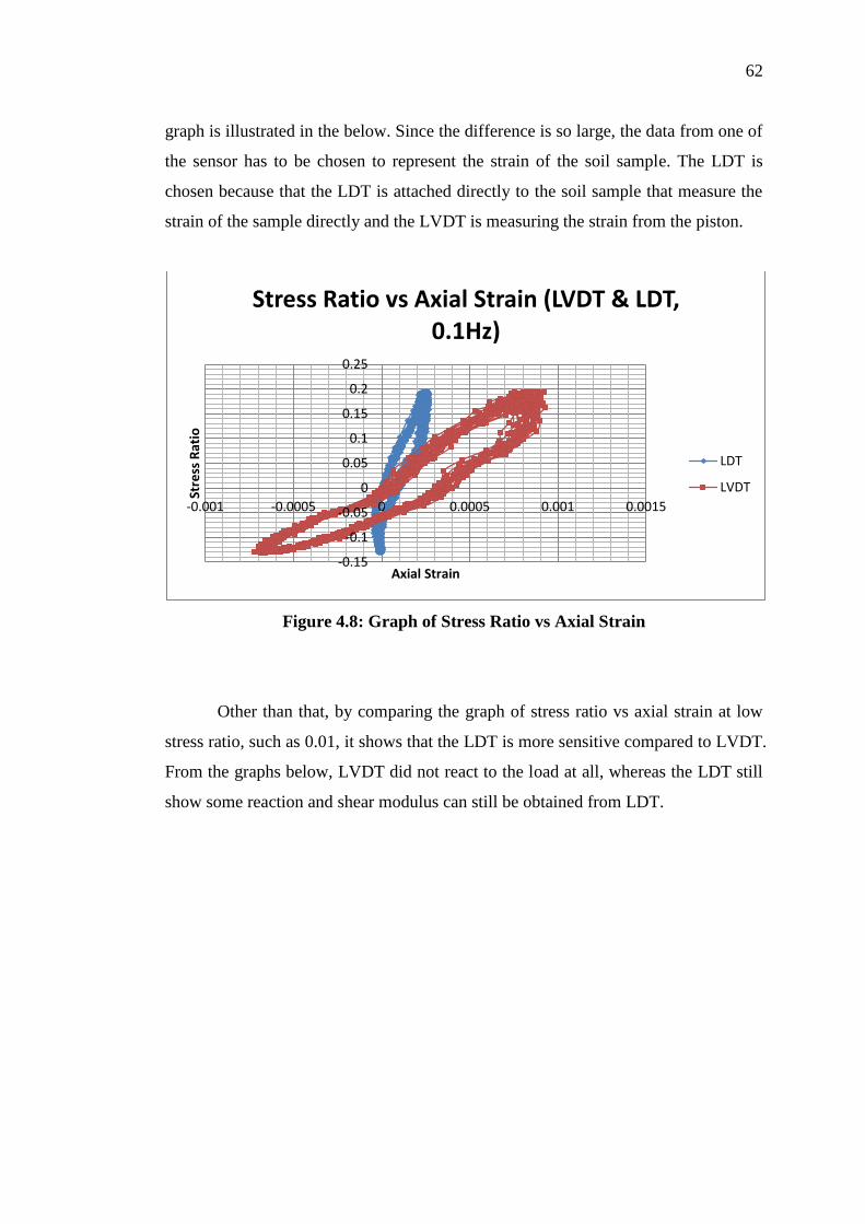
62

graph is illustrated in the below. Since the difference is so large, the data from one of

the sensor has to be chosen to represent the strain of the soil sample. The LDT is

chosen because that the LDT is attached directly to the soil sample that measure the

strain of the sample directly and the LVDT is measuring the strain from the piston.

Figure 4.8: Graph of Stress Ratio vs Axial Strain

Other than that, by comparing the graph of stress ratio vs axial strain at low

stress ratio, such as 0.01, it shows that the LDT is more sensitive compared to LVDT.

From the graphs below, LVDT did not react to the load at all, whereas the LDT still

show some reaction and shear modulus can still be obtained from LDT.

-0.15

-0.1

-0.05

0

0.05

0.1

0.15

0.2

0.25

-0.001 -0.0005 0 0.0005 0.001 0.0015

Stre

ss R

atio

Axial Strain

Stress Ratio vs Axial Strain (LVDT & LDT, 0.1Hz)

LDT

LVDT

63

Figure 4.9: Sensitivity of LVDT

Figure 4.10: Sensitivity of LDT

From the graph above, it shows that LDT can measure up to the strain of 10-6

,

whereas LVDT is not able to do it. Therefore, LDT is more reliable compared to

LVDT.

-0.015

-0.01

-0.005

0

0.005

0.01

0.015

-0.00004 -0.00002 0 0.00002 0.00004 0.00006 0.00008

Stre

ss R

atio

Axial Strain

Stress Ratio vs Axial Strain (LVDT, 0.1Hz)

y = 1.792346E+03x + 9.122636E-04

-0.015

-0.01

-0.005

0

0.005

0.01

0.015

-0.000006 -0.000004 -0.000002 0 0.000002 0.000004 0.000006

Stre

ss R

atio

Axial Strain

Stress Ratio vs Axial Strain (LDT, 0.1Hz)

64

By looking at the graph of stress ratio vs axial strain of LDT, for low stress

ratio, such as 0.01 to 0.10, no loop can be seen. For stress ratio after 0.12, the loop is

getting more and more obvious. Therefore, the soil can be said to be in the state of

elastic from stress ratio 0.01 to 0.10. However, after 0.12, the soil started to become

elasto-plastic.

Based on the study on Singapore residual soil by Tou (2003), the results are

compared with the residual soil studied by the author. Two different soils are tested

by Tou (2003). They are the Jurong Formation residual soils and Bukit Timah

Granite residual soil. Two samples are obtained from Jurong Formation residual soils

and labelled as JF1 and JF2, whereas the sample of Bukit Timah Granite residual

soils is labelled as BT. The basic index properties of all three soils are listed in the

table below.

Table 4.4: Basic Index Properties of JF and BT soils (Tou, 2003)

The residual soil from sedimentary Jurong Formation (JF1 and JF2) is

classified as CH in Unified Soil Classification System (USCS), whereas the residual

soil of Bukit Timah Granite (BT) is classified as SC, with significant sand content.

65

Besides, the experimental parameters for soil specimens JF1, JF2 and BT are listed in

the table below.

Table 4.5: Experimental Parameters for Soil Specimens JF1, JF2 and BT (Tou,

2003)

Tou (2003) concluded that the shear modulus reduces with the increase of

shear strain. This result shows the same trend found by the author on Shah Alam

residual soil. The figures below show the graph of shear modulus vs shear strain for

JF1, JF2 and BT from Tou (2003).

Figure 4.11: Graph of Shear Modulus vs Shear Strain for JF1 at 390 kPa

Consolidation Pressure (Tou, 2003)

66

Figure 4.12: Graph of Shear Modulus vs Shear Strain for JF2 at 290 kPa


Figure 4.13: Graph of Shear Modulus vs Shear Strain for BT at 290 kPa


67

On the other hand, Tou (2003) also presents that the damping ratio increases

as shear strain decreases for Singapore residual soil. This shows the same

relationship as the result from the author on Shah Alam residual soil. Figures below

show the graph of damping ratio vs shear strain of JF1, JF2 and BT.

Figure 4.14: Graph of Damping Ratio vs Shear Strain for JF1 at 390 kPa


Figure 4.15: Graph of Damping Ratio vs Shear Strain for JF2 at 290 kPa


68

Figure 4.16: Graph of Damping Ratio vs Shear Strain for BT at 290 kPa


Other than that, the Tou (2003) also commented that the shear modulus and

damping ratio at certain shear strain level increase as the frequency increases. This is

more obvious at small shear strain levels like 0.01 %, 0.02 % and 0.03 %. However,

the author observed no significant trend from Shah Alam residual soil to prove that

the frequency is affecting the shear modulus and damping ratio. From Tou's graph,

not all the data shows the increase of shear modulus and damping ratio with the

increase of frequency including some of the low shear strain level that is mentioned

by Tou (2003). There are still some fluctuations and the amount of fluctuation is

almost the same as the result obtained by the author for Shah Alam residual soil. The

figures below show the graph of shear modulus and damping ratio vs frequency by

Tou (2003).

69

Figure 4.17: Graph of Shear Modulus and Damping Ratio vs Frequency for JF1

70

Figure 4.18: Graph of Shear Modulus and Damping Ratio vs Frequency for JF2

71

Figure 4.19: Graph of Shear Modulus and Damping Ratio vs Frequency for BT

In addition, the author also plotted a graph of shear modulus vs shear strain

together with the result obtained from Tou (2003). The result of JF2 is chosen to be

compared with the result of the residual soil in Shah Alam because JF2 has lesser

technical problems occurred when the test is conducted (Tou, 2003). However, the

effective confining pressure of JF2 is only 47 kPa, whereas the confining pressure of

this research is 100 kPa. The relationship between the shear modulus and the

confining pressure can be expressed in the formula below (Ishihara, 1996).

(4.1)

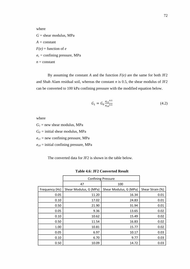
72

where

G = shear modulus, MPa

A = constant

F(e) = function of e

σc = confining pressure, MPa

n = constant

By assuming the constant A and the function F(e) are the same for both JF2

and Shah Alam residual soil, whereas the constant n is 0.5, the shear modulus of JF2

can be converted to 100 kPa confining pressure with the modified equation below.

(4.2)

where

G1 = new shear modulus, MPa

G0 = initial shear modulus, MPa

σc1 = new confining pressure, MPa

σc0 = initial confining pressure, MPa

The converted data for JF2 is shown in the table below.

Table 4.6: JF2 Converted Result

Confining Pressure

47 100

Frequency (Hz) Shear Modulus, G (MPa) Shear Modulus, G (MPa) Shear Strain (%)

0.05 11.20 16.34 0.01

0.10 17.02 24.83 0.01

0.50 21.90 31.94 0.01

0.05 9.36 13.65 0.02

0.10 10.62 15.49 0.02

0.50 11.54 16.83 0.02

1.00 10.81 15.77 0.02

0.05 6.97 10.17 0.03

0.10 6.70 9.77 0.03

0.50 10.09 14.72 0.03

73

1.00 11.62 16.95 0.03

2.00 9.83 14.34 0.03

0.05 4.00 5.83 0.10

0.10 4.42 6.45 0.10

0.50 3.91 5.70 0.10

1.00 4.70 6.86 0.10

2.00 6.60 9.63 0.10

0.05 2.77 4.04 0.20

0.10 2.27 3.31 0.20

0.50 3.00 4.38 0.20

1.00 2.09 3.05 0.20

2.00 2.38 3.47 0.20

0.05 1.42 2.07 0.30

0.10 1.85 2.70 0.30

0.50 1.36 1.98 0.30

1.00 1.89 2.76 0.30

2.00 2.05 2.99 0.30

0.05 0.80 1.17 1.00

0.10 0.43 0.63 1.00

0.50 0.60 0.88 1.00

1.00 0.41 0.60 1.00

2.00 0.60 0.88 1.00

Figure 4.20 and 4.21 are produced to compare the shear modulus from Tou

(2003) and this research by author. Figure 4.20 shows a direct comparison of the

shear modulus of JF2 with confining pressure of 47 kPa while the confining pressure

of 100 kPa is used in this research. In order to compare the shear modulus with the

same confining pressure, the shear modulus of JF2 was adjusted to 100 kPa as shown

above. Figure 4.21 below shows the comparison of shear modulus at the same

confining pressure of 100 kPa.

74

Figure 4.20: Comparing with JF2 (47 kPa)

Figure 4.21: Comparing with JF2 (100 kPa)

From these two figures, it is clearly shown that the shear modulus of the

residual soil from Shah Alam has much higher shear modulus compare to the JF2

soil in Singpoare.

0

20

40

60

80

100

120

140

0.0001 0.001 0.01 0.1 1

Shear Modulus (Mpa)

Shear Strain (%)


Shah Alam (100 kPa)

Jurong Formation (47 kPa)

0

20

40

60

80

100

120

140

0.0001 0.001 0.01 0.1 1

Shear Modulus (Mpa)

Shear Strain (%)


Shah Alam (100 kPa)

Jurong Formation (100 kPa)

75

4.4 Problems Encountered

In this section, all problems encountered by the author during this research will be

explained with the solutions. The major problem is the noise received by the USB-

6210 device from the sensors. This can really affect the result as the value is very

unstable. The noise can be generated from all kinds of electronic devices such as

laptop, power source, transformer, and amplifier.

This problem can be solved by grounding all the electronic devices. The

laptop can be grounded by using a USB cable and modified it with the other end

replaced by a crocodile clip. This cable can be plugged into the laptop easily and the

other end can be clipped to the transformer chassis. The transformer is also grounded

by connecting a wire to the chassis and the ground wire that is plugged into the

power supply. This creates a continuous flow and every electronic devices can be

grounded by simply connected to the chassis of the transformer.

To obsolete the noise from the laptop power supply, the power supply can be

turned off when the test carrying out. However, a constant check should be taken on

the laptop battery level to prevent the laptop from turning off in the process of testing.

In addition, there is also another problem with the LDT waterproofing. The

author tested the LDT in the water but the reading shows a very unstable value.

Therefore, the LDT is recoated with another layer of glue and a layer of paint is

sprayed on the wire connections. However, the LDT still failed to response normally

when submerged into the water. This problem is solved by consolidating the sample

with just the air pressure supplying to the triaxial cell without introducing water to

the cell.

76

Figure 4.22: LDT is Wrapped Up for Painting

Besides, some wire connections are easily be broken off. To solve this

problem, epoxy is used to cover the fragile part of the connection. Other than that,

epoxy is also used to seal the cable inside the water tank to prevent any leakage.

Plus, sometimes the LDT cannot be adjusted to the initial position, which is 1

mm deformation. To solve this problem, if the LDT is deformed less than 1 mm, a

hard plastic material can be placed in the clip to increase the deformation of LDT.

Therefore, it is always better to attach the LDT with the deformation lesser than 1

mm than more than 1 mm.

Other than that, if the specimen mould is not applied with oil, the soil sample

can be broken into half when removing the mould. Therefore, it is always advisable

to apply a layer of oil on the mould before compacting the soil.

77

Figure 4.23: Soil Sample Broken into Half

CHAPTER 5

5 CONCLUSIONS AND RECOMMENDATIONS

5.1 Conclusions

In conclusion, the frequency did not affect the shear modulus and damping ratio of

the residual soil tested herein. It was clearly shown that the shear modulus decreases

with the increase of stress ratio, whereas the damping ratio increases with the

increase of stress ratio. The relationship between shear modulus vs shear strain and

damping ratio vs shear strain of the tested residual soil is obtained.

5.2 Recommendations

To improve the quality of this research in the future, there are several things that

need to be improved. First of all, the Data Acquisition program and Air Pressure

Controller program need to be improved. This two programs are included in the CD

attached to this report. The data acquisition speed should be increased to obtain more

data, which will eventually provide a better result for high frequency test.

For the Air Pressure Controller program, the maximum frequency it can go is

1 Hz. If a higher frequency is used, the number of cycle performed will be lesser than

the cycle intended to perform due to some delay. This problem should be solved in

order to run the cyclic test with frequency higher than 1 Hz.

79

Plus, the LDT waterproofing should be improved as well. This might be done

by using epoxy to replace all the existing glue since epoxy is much stronger than the

glue. However, other better alternative can be used as well, because once the epoxy

is used, it will be permanent. Therefore, it is difficult to do some modification on the

connection in the future if needed.

Last but not least, a bigger space is needed for this research. The current

space is too small and everything has to be crammed together in a small space, which

is quite untidy.

80

REFERENCES

Boon, T. Y. (2013). Disaster risk reduction in malaysia and earthquake study based

on cyclic triaxial test. BSc thesis, Universiti Tunku Abdul Rahman.

British Standards Institution (1990). BS 1377-2:1990. Soils for civil engineering

purposes. Classification tests. London: BSI.

Doris, A. M. Y. and Hafez, M. A. (2011). 'Static laboratory compaction method',

Electronic Journal of Geotechnical Engineering, vol. 16, pp. 1589-1593.

Geotechnical Laboratory of DGM, (2004). Soil mechanics laboratory manual.

Jennifer, L. D., Jonathan, D. B., and Michael F. R. (2007). The liquefaction

susceptibility, resistance, and response of silty and clayey soils.

Ishihara, K., (1996). Soil behaviour in earthquake geotechnics, Oxford University

Press, New York, pp. 87.

Martin, D. L. (1990). A laboratory study of the effect of stress state on the elastic

moduli of sand. PhD thesis, The University of Texas at Austin.

Pieter, K. S. (1992). Implementation of a resonant column/torsional shear testing

apparatus. MSc thesis, North Carolina State University.

Rosaidi, C. A. (2001). 'Earthquake monitoring in malaysia'. Paper presented at the

Seismic Risk Seminar, Malaysia.

Sitharam, T. G. (2004). 'Dynamic properties and liquefaction potential of soils',

Current Science, vol. 87, no. 10, pp. 1370.

Sherliza, Z. S., Sumio, S., and Hiroyuki, G. (2012). 'Proposal for seismic resistant

design in malaysia: assessment of possible ground motions in peninsular malaysia',

Annual Report of Disaster Prevention Research Institute Kyoto University, no.

55b.

Tou, J. H. (2003). Cyclic triaxial test apparatus for evaluating dynamic properties of

residual soils. MSc thesis, Nanyang Technological University.

81

Transducer Techniques, (n.d.). Quater bridge, half bridge and full wheatstone bridge

strain gauge load cell configurations. Available from:

<http://www.transducertechniques.com/wheatstone-bridge.aspx>. [19 April 2013].

82

APPENDICES

APPENDIX A: Calibration of Air Pressure Transducer

Air pressure (bar) Voltage supply (v) Voltage difference (v)

1 2.9 1.25879

1.5 3.5 1.85879

2 4.1 2.45879

2.5 4.7 3.05879

3 5.3 3.65879

3.5 5.95 4.30879

4 6.55 4.90879

4.5 7.2 5.55879

5 7.85 6.20879

4.5 7.2 5.55879

4 6.55 4.90879

3.5 5.95 4.30879

3 5.3 3.65879

2.5 4.7 3.05879

2 4.1 2.45879

1.5 3.5 1.85879

1 2.9 1.25879

83

y = 1.231621E+00x + 4.566210E-08 R² = 9.997712E-01

0

1

2

3

4

5

6

7

0 1 2 3 4 5 6

Voltage Difference (v)

Air Pressure (bar)

Graph of Voltage Difference vs Air Pressure

84

APPENDIX B: Calibration of Load Cell Limit

Mass (kg) Strain (µε)

Strain (µε)

0 39 0

4.988 10 -29

9.9825 -20 -59

14.9465 -53 -92

9.9825 -22 -61

4.988 9 -30

0 36 -3

By using the equation from the graph, if maximum strain is 3000 µε, then the load

will be 497.72 kg.

y = -1.659346E-01x - 8.265608E-02 R² = 9.978899E-01

-5

0

5

10

15

20

25

30

35

-250 -200 -150 -100 -50 0

Mass (kg)

Strain (µε)

Graph of Mass vs Strain

85

APPENDIX C: Calibration of Load Cell

Mass (g) Cumulative Mass (g) Voltage (v) Voltage Different (v)

0 0 4.58 -0.00194

10136.5 10136.5 4.22 -0.36194

9939 20075.5 3.87 -0.71194

10065 30140.5 3.5 -1.08194

9935 40075.5 3.14 -1.44194

9895 49970.5 2.78 -1.80194

9998 59968.5 2.42 -2.16194

4994.5 64963 2.25 -2.33194

4987.5 69950.5 2.14 -2.44194

4963 74913.5 1.96 -2.62194

4960 79873.5 1.79 -2.79194

4960 79873.5 1.79 -2.79194

4963 74913.5 1.95 -2.63194

4987.5 69950.5 2.12 -2.46194

4994.5 64963 2.29 -2.29194

9998 59968.5 2.47 -2.11194

9895 49970.5 2.82 -1.76194

9935 40075.5 3.18 -1.40194

10065 30140.5 3.53 -1.05194

9939 20075.5 3.89 -0.69194

10136.5 10136.5 4.25 -0.33194

0 0 4.6 0.01806

86

y = -3.525791E-05x + 4.581940E+00 R² = 9.994327E-01

1

1.5

2

2.5

3

3.5

4

4.5

5

0 20000 40000 60000 80000 100000

Voltage (v)

Mass (g)

Graph of Voltage vs Mass

Case 2

Linear (Case 2)

87

APPENDIX D: Calibration of Air Pressure Transducer with Load Cell

Air pressure (bar) Voltage (v) Mass of Load (g) Mass of Load (kg)

0 4.54 0 0

0.5 3.66 24958.93829 24.95893829

1 2.83 48499.75509 48.49975509

1.5 2.03 71189.69899 71.18969899

2 1.25 93312.3943 93.3123943

2.5 0.37 118271.3326 118.2713326

2.5 0.27 121107.5756 121.1075756

2 0.98 100970.2504 100.9702504

1.5 1.9 74876.81488 74.87681488

1 2.68 52754.11957 52.75411957

0.5 3.58 27227.93268 27.22793268

0 4.46 2268.99439 2.26899439

0.5 3.64 25526.18689 25.52618689

1 2.81 49067.00369 49.06700369

1.5 1.95 73458.69338 73.45869338

2 1.12 96999.51018 96.99951018

2.5 0.27 121107.5756 121.1075756

2 1.14 96432.26158 96.43226158

1.5 1.88 75444.06347 75.44406347

1 2.73 51335.99808 51.33599808

0.5 3.36 33467.66726 33.46766726

0 4.28 7374.231768 7.374231768

0 4.36 5105.237378 5.105237378

0.5 3.59 26944.30838 26.94430838

1 2.71 51903.24668 51.90324668

1.5 1.91 74593.19058 74.59319058

2 1.07 98417.63167 98.41763167

2.5 0.27 121107.5756 121.1075756

2 0.98 100970.2504 100.9702504

1.5 1.81 77429.43357 77.42943357

1 2.65 53604.99247 53.60499247

0.5 3.56 27795.18128 27.79518128

0 4.43 3119.867287 3.119867287

88

y = 4.678143E+01x + 4.102566E+00 R² = 9.963288E-01

0

20

40

60

80

100

120

140

0 0.5 1 1.5 2 2.5 3

Mass of Load (kg)

Air Pressure (bar)

Graph of Mass of Load vs Air Pressure

89

APPENDIX E: Calibration of LVDT

Dail gauge reading (0.01mm) Voltage

(v)

0 0.59

25 0.75

50 0.92

75 1.08

100 1.24

125 1.4

150 1.57

175 1.73

200 1.89

225 2.06

250 2.22

275 2.39

300 2.55

325 2.71

350 2.88

375 3.04

400 3.2

425 3.36

450 3.53

475 3.69

500 3.85

525 4.01

550 4.18

575 4.34

600 4.5

600 4.5

575 4.34

550 4.17

525 4.01

500 3.85

475 3.69

450 3.52

90

425 3.36

400 3.2

375 3.03

350 2.87

325 2.7

300 2.54

275 2.38

250 2.21

225 2.05

200 1.89

175 1.72

150 1.56

125 1.39

100 1.23

75 1.07

50 0.91

25 0.75

0 0.58

0 0.58

25 0.74

50 0.91

75 1.07

100 1.23

125 1.39

150 1.56

175 1.72

200 1.88

225 2.05

250 2.21

275 2.38

300 2.54

325 2.7

350 2.87

375 3.03

400 3.2

425 3.36

450 3.52

475 3.69

500 3.84

525 4.01

550 4.17

91

575 4.33

600 4.5

y = 6.531692E-03x + 5.828923E-01 R² = 9.999818E-01

0

0.5

1

1.5

2

2.5

3

3.5

4

4.5

5

0 100 200 300 400 500 600 700

Voltage (V)

Dail Gauge Reading (0.01mm)

Graph of Voltage vs Dail Gauge Reading

92

APPENDIX F: Calibration of LDT Initial Position

Dail gauge reading (0.01mm) Strain (µε)

0 -585

15 -122

30 430

45 931

60 1364

75 1715

90 2014

105 2280

120 2527

135 2748

From the equation of the graph, 1 mm deformation is 2218 µε.

y = -1.022391E-01x2 + 3.860631E+01x - 6.201182E+02 R² = 9.993000E-01

-1000

0

1000

2000

3000

0 20 40 60 80 100 120 140 160

Strain (µε)

Deformation (0.01mm)

Graph of Strain vs Deformation

93

APPENDIX G: Calibration of LDT

Case 1:

Case 2: Deformation

(0.01mm) Amplified Voltage (v)


Amplified Voltage (v)

150 -9.8

100 -7.09

145 -9.48

101 -7.2

140 -9.23

102 -7.27

135 -8.96

103 -7.33

130 -8.71

104 -7.37

125 -8.48

105 -7.44

120 -8.21

106 -7.49

115 -7.96

107 -7.55

110 -7.67

108 -7.6

105 -7.4

109 -7.67

100 -7.14

110 -7.73

105 -7.49

109 -7.63

110 -7.73

108 -7.55

115 -8.02

107 -7.49

120 -8.29

106 -7.42

125 -8.55

105 -7.37

130 -8.82

104 -7.32

135 -9.06

103 -7.25

140 -9.28

102 -7.21

145 -9.55

101 -7.14

150 -9.78

100 -7.08

145 -9.44 140 -9.23 135 -8.94 130 -8.69 125 -8.43 120 -8.17 115 -7.91 110 -7.63 105 -7.38 100 -7.09

94

Case 1 is for large strain calibration and Case 2 is for small strain calibration.

y = 3.687897E-01x2 - 1.277766E+01x - 9.882959E+00

R² = 9.965836E-01

y = 1.178548E-01x2 - 1.432758E+01x - 7.566959E+00

R² = 9.736475E-01 90

100

110

120

130

140

150

160

-10 -9 -8 -7 -6


Voltage (v)

Graph of Deformation vs Voltage

Larger strain

Smaller strain

Poly. (Larger strain)

Poly. (Smaller strain)

95

APPENDIX H: Test Specimen Data

Unit

Density 16 kN/m3

Diameter 100 mm

Heigh 200 mm

Volume 1570796 mm3

0.001571 m3

Area 7853.982 mm2

0.007854 m2

Mass of soil needed 0.025133 kN

2.513274 kg

Mass of 20% water 0.502655 kg

Specimen dimension (Before testing)

Diameter (mm)

Top 100.140000

99.850000

Bottom 100.450000

99.990000

Height (mm)

200.710000

200.400000

199.690000

Mass (g) 3083.500000

Average Diameter (mm) 100.107500

Average Height (mm) 200.266667

Area (mm2) 7870.876771

Area (m2) 0.007871

Specimen dimension (After testing)

Diameter (mm)

Top

98.160000

96.680000

96.060000

Bottom

99.190000

100.350000

100.330000

Height (mm) 199.690000

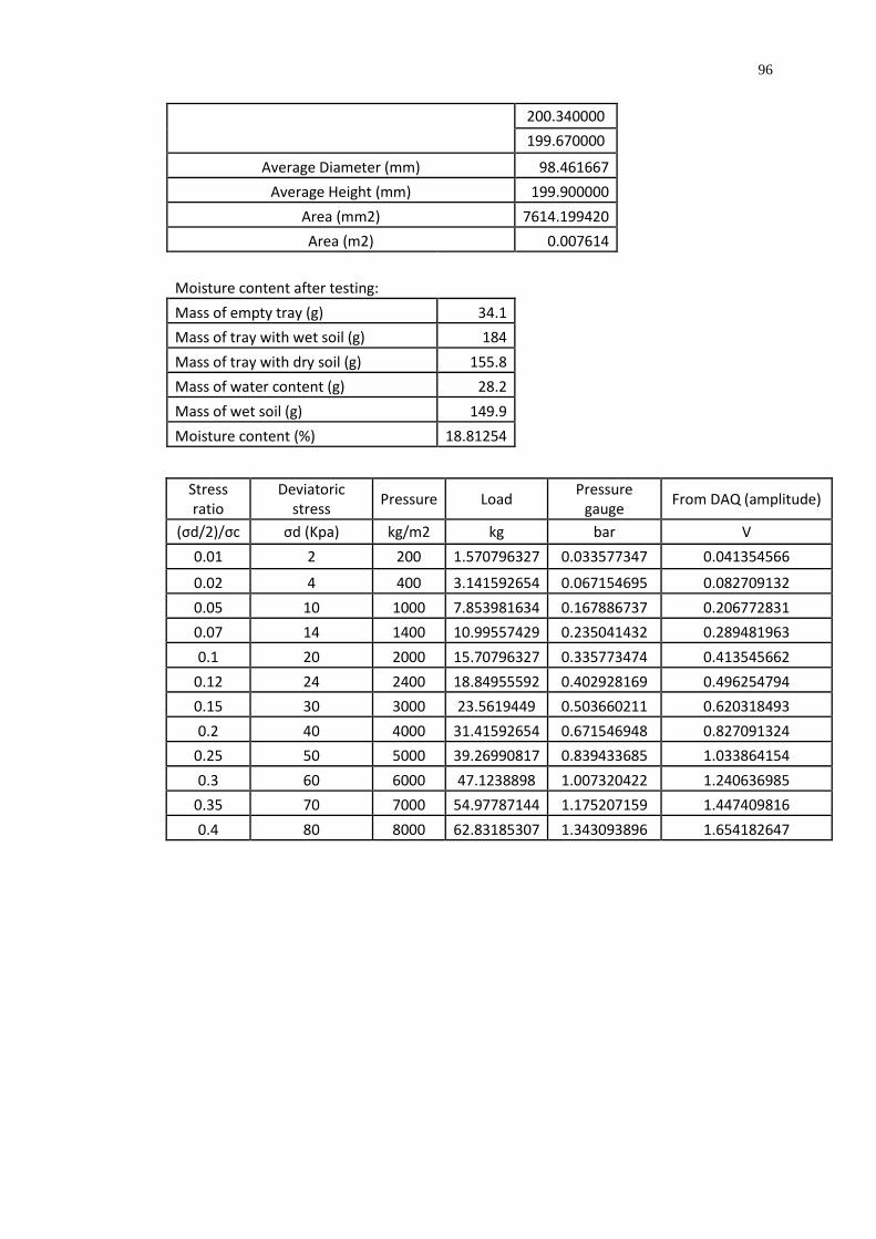
96

200.340000

199.670000

Average Diameter (mm) 98.461667

Average Height (mm) 199.900000

Area (mm2) 7614.199420

Area (m2) 0.007614

Moisture content after testing: Mass of empty tray (g) 34.1

Mass of tray with wet soil (g) 184 Mass of tray with dry soil (g) 155.8 Mass of water content (g) 28.2 Mass of wet soil (g) 149.9 Moisture content (%) 18.81254

Stress ratio

Deviatoric stress

Pressure Load Pressure

gauge From DAQ (amplitude)

(σd/2)/σc σd (Kpa) kg/m2 kg bar V

0.01 2 200 1.570796327 0.033577347 0.041354566

0.02 4 400 3.141592654 0.067154695 0.082709132

0.05 10 1000 7.853981634 0.167886737 0.206772831

0.07 14 1400 10.99557429 0.235041432 0.289481963

0.1 20 2000 15.70796327 0.335773474 0.413545662

0.12 24 2400 18.84955592 0.402928169 0.496254794

0.15 30 3000 23.5619449 0.503660211 0.620318493

0.2 40 4000 31.41592654 0.671546948 0.827091324

0.25 50 5000 39.26990817 0.839433685 1.033864154

0.3 60 6000 47.1238898 1.007320422 1.240636985

0.35 70 7000 54.97787144 1.175207159 1.447409816

0.4 80 8000 62.83185307 1.343093896 1.654182647

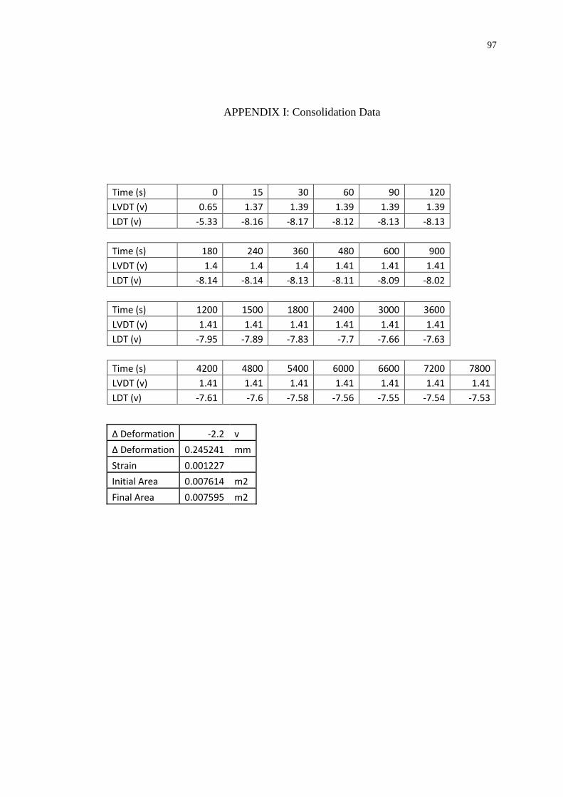
97

APPENDIX I: Consolidation Data

Time (s) 0 15 30 60 90 120 LVDT (v) 0.65 1.37 1.39 1.39 1.39 1.39 LDT (v) -5.33 -8.16 -8.17 -8.12 -8.13 -8.13

Time (s) 180 240 360 480 600 900 LVDT (v) 1.4 1.4 1.4 1.41 1.41 1.41 LDT (v) -8.14 -8.14 -8.13 -8.11 -8.09 -8.02

Time (s) 1200 1500 1800 2400 3000 3600 LVDT (v) 1.41 1.41 1.41 1.41 1.41 1.41 LDT (v) -7.95 -7.89 -7.83 -7.7 -7.66 -7.63

Time (s) 4200 4800 5400 6000 6600 7200 7800

LVDT (v) 1.41 1.41 1.41 1.41 1.41 1.41 1.41

LDT (v) -7.61 -7.6 -7.58 -7.56 -7.55 -7.54 -7.53

Δ Deformation -2.2 v

Δ Deformation 0.245241 mm

Strain 0.001227

Initial Area 0.007614 m2

Final Area 0.007595 m2

98

1.365

1.37

1.375

1.38

1.385

1.39

1.395

1.4

1.405

1.41

1.415

1 10 100 1000 10000

Voltage (v)

Time (s)

Graph of LVDT Voltage vs Time

LVDT

-8.5

-8

-7.5

-7

-6.5

-6

-5.5

-5

1 10 100 1000 10000

Voltage (v)

Time (s)

Graph of LDT Voltage vs Time

LDT

disaster risk reduction in malaysia and …eprints.utar.edu.my/851/1/ci-2013-0907674-1.pdfdisaster...

Documents