directional multiscale processing of images …dlabate/nonsub_composite_fin.pdf · directional...
TRANSCRIPT
DIRECTIONAL MULTISCALE PROCESSING OF IMAGES
USING WAVELETS WITH COMPOSITE DILATIONS
GLENN R. EASLEY, DEMETRIO LABATE, VISHAL M. PATEL
Abstract. It is widely recognized that the performance of many image pro-
cessing algorithms can be significantly improved by applying multiscale image
representations with the ability to handle very efficiently directional and other
geometric features. Wavelets with composite dilations offer a flexible and espe-
cially effective framework for the construction of such representations. Unlike
traditional wavelets, this approach enables the construction of waveforms rang-
ing not only over various scales and locations but also over various orientations
and other orthogonal transformations. Several useful constructions are derived
from this approach, including the well-known shearlet representation and new
ones, introduced in this paper. In this work, we introduce and apply a novel
multiscale image decomposition algorithm for the efficient digital implementa-
tion of wavelets with composite dilations. Due to its ability to handle geomet-
ric features efficiently, our new image processing algorithms provide consistent
improvements upon competing state-of-the-art methods, as illustrated on a
number of image denoising and image enhancement demonstrations.
1. Introduction
It has become commonly understood that while 1D wavelets are optimal at ap-
proximating point singularities, their 2D separable counterparts are not equally
effective at approximating singularities along curves which model edges in images.
The need for directional filtering in order to improve multidimensional data process-
ing was early recognized, for example, in the works [1, 23, 41]. More recently, new
Key words and phrases. Wavelets, directional filter banks, wavelets with composite dilations,contourlets, shearlets, curvelets.
1

2 GLENN R. EASLEY, DEMETRIO LABATE, VISHAL M. PATEL
generations of directional representations were developed which exhibit near opti-
mal approximations on the class of cartoon images. The most notable of these rep-
resentations are the curvelets [42, 8], the contourlets [13] and the shearlets [26, 34],
which are constructed by defining systems of analyzing waveforms ranging not only
at various scales and locations, like traditional wavelets, but also at various orien-
tations, with the number of orientations increasing at finer scales.
Within the context of improved multidimensional representations, the theory
of wavelets with composite dilations, originally developed in [26, 27, 28], is espe-
cially important. This framework is a generalization of the classical theory from
which traditional wavelets are derived, and it provides a very flexible setting for the
construction of many truly multidimensional variants of wavelets, such as the well
known construction of shearlets 1. Several additional sophisticated constructions
using this approach were obtained by Blanchard [4, 5], by Kryshtal and Blanchard
in a paper which exploits the connection with crystallographic groups [6], and by
Kryshtal et al. [32]. Furthermore, it was recently shown by two of the authors in [16]
that several recent filter bank constructions such as the hybrid wavelets of Eslami
and Rada [20, 21, 22] and the variants of the contourlets construction proposed
in [31, 45] can either be derived or are closely related to systems obtained from the
framework of wavelets with composite dilations.
These observations indicate the potential of wavelets with composite dilations
for the construction of directional multiscale representations going far beyond tra-
ditional wavelets with respect to their ability to represent geometric features. How-
ever, except for some very special cases, no satisfactory method for designing effi-
cient numerical implementations of wavelets with composite dilations was developed
so far, due to the difficulty of adapting the standard wavelet implementation al-
gorithms to this more general setting. The goal of this paper is to introduce a
1Even though the shearlet system is not exactly an example of wavelets with composite dila-tions, it is closely related to this framework being defined as a union of two such systems [26, 34].
WAVELETS WITH COMPOSITE DILATIONS 3
new general procedure for the design of discrete multiscale transforms which takes
full advantage of the geometric features associated with the framework of wavelets
with composite dilations. Using this approach, we are able to design and implement
several new classes of directional discrete transforms and to obtain improved imple-
mentations of known ones. As will be illustrated in this paper, the newly derived
algorithms based on wavelets with composite dilations are highly competitive in
imaging applications such as denoising and enhancement.
Recall that, for tasks such as image denoising and enhancement, where the ob-
jective is to extract or emphasize certain image features, it is often beneficial to
use redundant representations. A standard method for designing nonsubsampled
directional representations is to use critically sampled transformations based on
2D directional filters that satisfies Bezout’s identity, as done in [12, 22]. As will
become clear below, this approach is frequently associated with filters that do not
faithfully match with the desired theoretical frequency decomposition. By contrast,
in this paper we introduce a novel filter bank construction technique that enables
the projection of the data directly onto the desired directionally-oriented frequency
subbands. A key new feature of our construction is the ability to generate the
transform coefficients by directly applying the action of the matrices associated
with the frequency plane decomposition. This is in contrast to earlier implementa-
tions such as the discrete shearlet transform in [17], which was designed to mimic
the desired frequency plane decomposition. Not only does our new approach follow
directly from the theoretical setting, but it also allows for more sophisticated com-
posite wavelet decompositions enabling a much finer handling of the geometry in
the data. As special cases of our approach, we obtain an improved implementation
of the shearlet transform and we introduce new hyperbolic composite wavelet trans-
form. This last transform has potentially high impact in deconvolution and other
image enhancement applications, as indicated by the novel decompositions sug-
gested in [10] and by the techniques for dealing with motion blur recently proposed

4 GLENN R. EASLEY, DEMETRIO LABATE, VISHAL M. PATEL
in [19]. This is due to the special decomposition of the frequency plane associated
with this transform which provides a somewhat finer partition of the low-frequency
region vs. the high-frequency one.
Finally, we wish to mention the important work by Durand [15], who explores
a large family of (discrete) directional wavelets and derives their implementation
from a single nonseparable filter bank structure. With respect to our approach
which is continuous (i.e., we deal with functions in L2(R2)), the work of Durand is
purely discrete.
1.1. Paper Organization. The definition and basic properties of wavelets with
composite dilations, along with novel constructions are presented in Section 2. The
novel discrete implementations are discussed in Section 3. Numerical demonstra-
tions illustrating the performance of the new constructions for denoising and image
enhancement are presented in Section 4. Concluding remarks are given in Section 5.
2. Wavelets with composite dilations
Let us introduce the notation which will be used subsequently. Given τ ∈ Rn,
the translation operator Tτ on L2(Rn) is defined by
Tτ f(x) = f(x− τ), x ∈ Rn, f ∈ L2(Rn).
For a ∈ GLn(R) (where GLn(R) denotes the group of invertible matrices on Rn),
the dilation operator Da is given by
Da f(x) = |det a|−1/2 f(a−1x).
We adopt the convention that the points x ∈ Rn are column vectors and the points
ξ ∈ Rn (the Fourier domain) are row vectors. Hence a vector x ∈ Rn multiplying a
matrix a ∈ GLn(R) on the right is a column vector and a vector ξ ∈ Rn multiplying
a matrix a ∈ GLn(R) on the left is a row vector; that is, ax ∈ Rn and ξa ∈ Rn.
Notice that we will denote matrices as lower-case letters, and use capital letters to

WAVELETS WITH COMPOSITE DILATIONS 5
denote sets. The Fourier transform of f ∈ L2(Rn) is given by
f(ξ) =
∫Rn
f(x) e−2πiξx dx,
where ξ ∈ Rn and the inverse Fourier transform is
f(x) =
∫Rn
f(ξ) e2πiξx dξ.
The standard wavelet systems generated by Ψ = {ψ1, . . . , ψL} ⊂ L2(Rn) and
A = {ai : i ∈ Z} are the collections of functions of the form
{Dja Tk ψm : j ∈ Z, k ∈ Zn,m = 1, . . . , L},
which form a Parseval frame for L2(Rn). That is, for all f ∈ L2(Rn), we have:2
∥f∥2 =∑j∈Z
∑k∈Zn
L∑m=1
|⟨f,Dja Tk ψm⟩|2.
Note that the traditional wavelet systems are obtained with a = 2 I, where I is the
identity matrix. That is, the dilation factor is the same for all coordinate axes.
The wavelets with composite dilations [26] overcome the limitations of standard
wavelets in dealing with the geometry of multivariate functions by including a
second set of dilations. Namely, they have the form
AAB(Ψ) = {DaDb Tk Ψ : k ∈ Zn, a ∈ A, b ∈ B},
whereA, B are countable subsets ofGLn(R) and the matrices b ∈ B satisfy | det b| =
1. As for standard wavelet systems, Ψ = {ψ1, . . . , ψL} ⊂ L2(Rn) chosen so that
∥f∥2 =∑a∈A
∑b∈B
∑k∈Zn
L∑m=1
|⟨f,DaDb Tkψm⟩|2,
2Recall that an orthonormal basis is a special case of a Parseval frame; however, the elementsof a Parseval frame need not be orthogonal.
6 GLENN R. EASLEY, DEMETRIO LABATE, VISHAL M. PATEL
for any f ∈ L2(Rn). Usually, the matrices a ∈ A are expanding (but not necessarily
isotropic, as in the traditional wavelet case); the matrices b ∈ B, which are non-
expanding, are associated with rotations and other orthogonal transformations. As
a result, one can define systems of wavelets with composite dilations containing
elements that are “long and narrow” and range over many locations, scales, shapes
and directions. Building on this idea [26, 34], shearlets are able to provide a nearly
optimally sparse representation for a general class of images [24, 25].
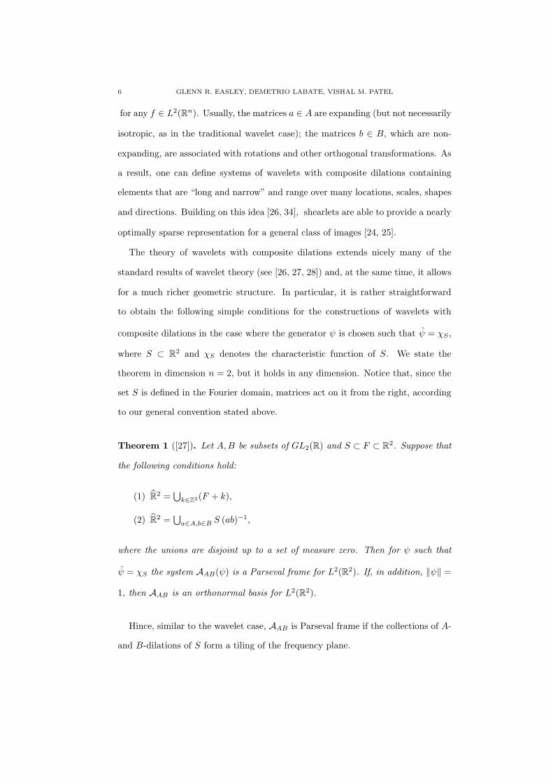
The theory of wavelets with composite dilations extends nicely many of the
standard results of wavelet theory (see [26, 27, 28]) and, at the same time, it allows
for a much richer geometric structure. In particular, it is rather straightforward
to obtain the following simple conditions for the constructions of wavelets with
composite dilations in the case where the generator ψ is chosen such that ψ = χS ,
where S ⊂ R2 and χS denotes the characteristic function of S. We state the
theorem in dimension n = 2, but it holds in any dimension. Notice that, since the
set S is defined in the Fourier domain, matrices act on it from the right, according
to our general convention stated above.
Theorem 1 ([27]). Let A,B be subsets of GL2(R) and S ⊂ F ⊂ R2. Suppose that
the following conditions hold:
(1) R2 =∪
k∈Z2(F + k),
(2) R2 =∪
a∈A,b∈B S (ab)−1,
where the unions are disjoint up to a set of measure zero. Then for ψ such that
ψ = χS the system AAB(ψ) is a Parseval frame for L2(R2). If, in addition, ∥ψ∥ =
1, then AAB is an orthonormal basis for L2(R2).
Hince, similar to the wavelet case, AAB is Parseval frame if the collections of A-
and B-dilations of S form a tiling of the frequency plane.
WAVELETS WITH COMPOSITE DILATIONS 7
It is clear that the systems described in Theorem 1 are not well-localized in
the spatial domain, since their elements are characteristic functions of sets in the
frequency domain and, hence, have slow spatial decay. Wavelets with composite
dilations which are well-localized require ad hoc constructions such as the shearlets
in [24] or the constructions described in [16]. Some new well-localized constructions
will be introduced in this paper.
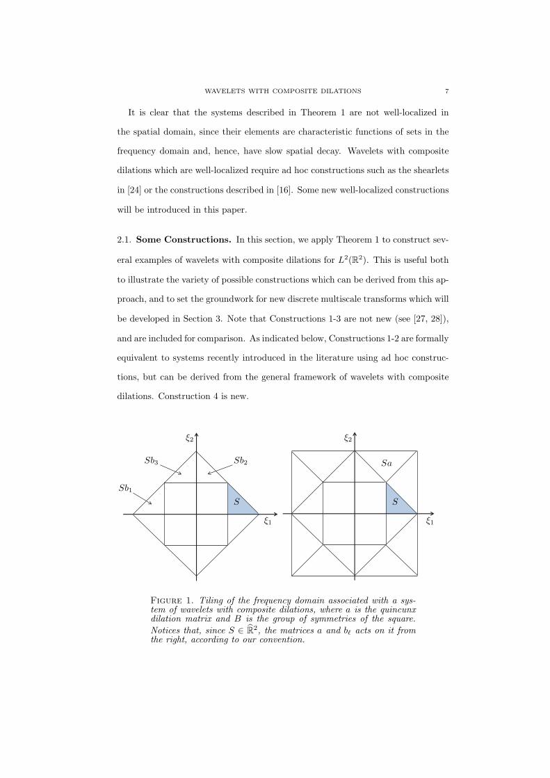
2.1. Some Constructions. In this section, we apply Theorem 1 to construct sev-
eral examples of wavelets with composite dilations for L2(R2). This is useful both
to illustrate the variety of possible constructions which can be derived from this ap-
proach, and to set the groundwork for new discrete multiscale transforms which will
be developed in Section 3. Note that Constructions 1-3 are not new (see [27, 28]),
and are included for comparison. As indicated below, Constructions 1-2 are formally
equivalent to systems recently introduced in the literature using ad hoc construc-
tions, but can be derived from the general framework of wavelets with composite
dilations. Construction 4 is new.
Sb1
Sb3
ξ2
Sb2
S
ξ1 ξ1
S
Sa
ξ2
Figure 1. Tiling of the frequency domain associated with a sys-tem of wavelets with composite dilations, where a is the quincunxdilation matrix and B is the group of symmetries of the square.
Notices that, since S ∈ R2, the matrices a and bℓ acts on it fromthe right, according to our convention.

8 GLENN R. EASLEY, DEMETRIO LABATE, VISHAL M. PATEL
2.1.1. Construction 1. Let A = {aj : j ∈ Z} where a = ( 1 1−1 1 ) (the quincunx ma-
trix) and letB be the group of symmetries of the square, that is, B = {±b0,±b1,±b2,±b3}
where b0 = ( 1 00 1 ), b1 = ( 1 0
0 −1 ), b2 = ( 0 11 0 ), b3 = ( 0 −1
−1 0 ). Let ψ(ξ) = χS(ξ),
where the set S is the union of the triangles with vertices (1, 0), (2, 0), (1, 1) and
(−1, 0), (−2, 0), (−1,−1), which is illustrated in Figure 1. A direct calculation shows
that S satisfies the assumptions of Theorem 1, so that the system
AAB(ψ) = {DjaDb Tk ψ : j ∈ Z, b ∈ B, k ∈ Z2}
is an orthonormal basis for L2(R2) (in fact, it is a Parseval frame and ∥ψ∥ = 1).
As noticed in [16], the frequency partition achieved by the Hybrid Quincunx
Wavelet Directional Transform (HQWDT) from [22] is a simple modification of
this construction, which is obtained by splitting each triangle of the set S into
2 smaller triangles. Another example, with the same matrices A and B, but a
different generating set S, is illustrated in Figure 2 on the left. For future labeling,
we will refer to this second construction concisely as the ab-star decomposition
alluding to its star-like frequency tiling and its composite wavelet origin.
2.1.2. Construction 2. Let A = {aj : j ∈ Z} where a = ( 2 00 2 ) and consider B =
{b0, b1, b2, b3} where b0 = ( 1 00 1 ), b1 = ( 1 0
0 −1 ), b2 = ( 0 11 0 ), b3 = ( 0 −1
−1 0 ). Let R be the
union of the trapezoid with vertices (1, 0), (2, 0), (1, 1), (2, 2) and the symmetric one
with vertices (−1, 0), (−2, 0), (−1,−1), (−2,−2). Next, we partition each trapezoid
into right triangles Rm, m = 1, 2, 3, as illustrated in Figure 2 on the right. Hence
we define Ψ = {ψm : m = 1, 2, 3}, where ψm(ξ) = χRm(ξ). Then the system
AAB(Ψ) = {DjaDb Tk Ψ : j ∈ Z, b ∈ B, k ∈ Z2}
is an orthonormal basis for L2(R2).
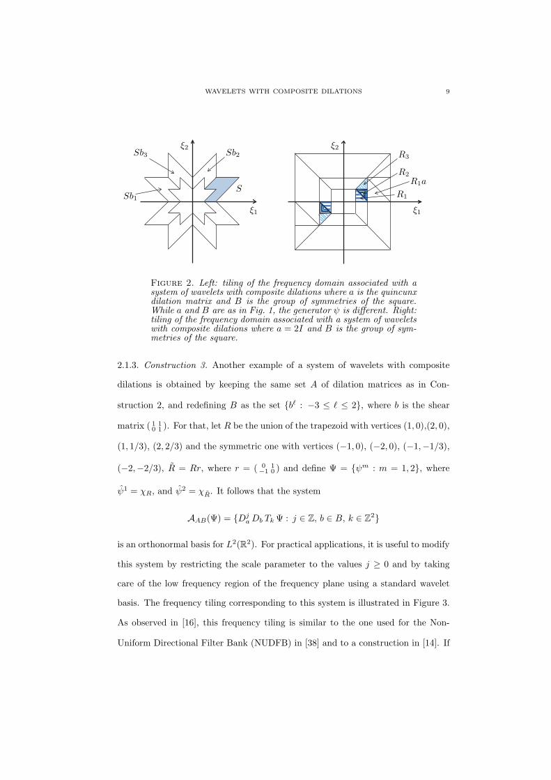
WAVELETS WITH COMPOSITE DILATIONS 9
ξ1
ξ2
ξ1
Sb1
Sb3 Sb2
S
ξ2R3
R2
R1
R1a
Figure 2. Left: tiling of the frequency domain associated with asystem of wavelets with composite dilations where a is the quincunxdilation matrix and B is the group of symmetries of the square.While a and B are as in Fig. 1, the generator ψ is different. Right:tiling of the frequency domain associated with a system of waveletswith composite dilations where a = 2I and B is the group of sym-metries of the square.
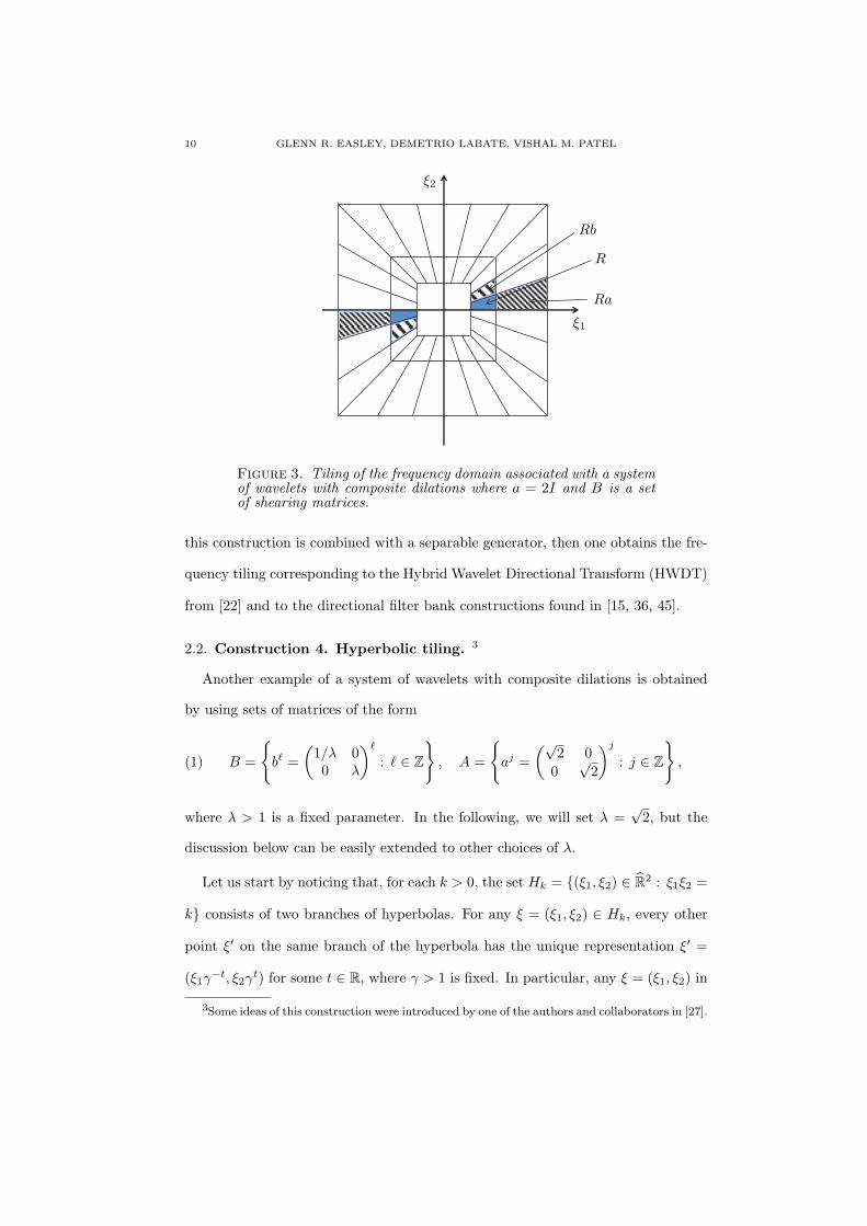
2.1.3. Construction 3. Another example of a system of wavelets with composite
dilations is obtained by keeping the same set A of dilation matrices as in Con-
struction 2, and redefining B as the set {bℓ : −3 ≤ ℓ ≤ 2}, where b is the shear
matrix ( 1 10 1 ). For that, let R be the union of the trapezoid with vertices (1, 0),(2, 0),
(1, 1/3), (2, 2/3) and the symmetric one with vertices (−1, 0), (−2, 0), (−1,−1/3),
(−2,−2/3), R = Rr, where r = ( 0 1−1 0 ) and define Ψ = {ψm : m = 1, 2}, where
ψ1 = χR, and ψ2 = χR. It follows that the system
AAB(Ψ) = {DjaDb Tk Ψ : j ∈ Z, b ∈ B, k ∈ Z2}
is an orthonormal basis for L2(R2). For practical applications, it is useful to modify
this system by restricting the scale parameter to the values j ≥ 0 and by taking
care of the low frequency region of the frequency plane using a standard wavelet
basis. The frequency tiling corresponding to this system is illustrated in Figure 3.
As observed in [16], this frequency tiling is similar to the one used for the Non-
Uniform Directional Filter Bank (NUDFB) in [38] and to a construction in [14]. If
10 GLENN R. EASLEY, DEMETRIO LABATE, VISHAL M. PATEL
ξ2
Rb
R
Ra
ξ1
Figure 3. Tiling of the frequency domain associated with a systemof wavelets with composite dilations where a = 2I and B is a setof shearing matrices.
this construction is combined with a separable generator, then one obtains the fre-
quency tiling corresponding to the Hybrid Wavelet Directional Transform (HWDT)
from [22] and to the directional filter bank constructions found in [15, 36, 45].
2.2. Construction 4. Hyperbolic tiling. 3
Another example of a system of wavelets with composite dilations is obtained
by using sets of matrices of the form
(1) B =
{bℓ =
(1/λ 00 λ
)ℓ
: ℓ ∈ Z
}, A =
{aj =
(√2 0
0√2
)j
: j ∈ Z
},
where λ > 1 is a fixed parameter. In the following, we will set λ =√2, but the
discussion below can be easily extended to other choices of λ.
Let us start by noticing that, for each k > 0, the set Hk = {(ξ1, ξ2) ∈ R2 : ξ1ξ2 =
k} consists of two branches of hyperbolas. For any ξ = (ξ1, ξ2) ∈ Hk, every other
point ξ′ on the same branch of the hyperbola has the unique representation ξ′ =
(ξ1γ−t, ξ2γ
t) for some t ∈ R, where γ > 1 is fixed. In particular, any ξ = (ξ1, ξ2) in
3Some ideas of this construction were introduced by one of the authors and collaborators in [27].

WAVELETS WITH COMPOSITE DILATIONS 11
S
Sb Sa
ξ2/ξ1 = 4
ξ2/ξ1 = 2ξ2ξ1 = 1
ξ2ξ1 = 4
ξ2ξ1 = 2ξ2ξ1 = 1
ξ2
ξ1 r
2t
S
Sb
Sa
Figure 4. The figure on the left shows the hyperbolic trapezoidS = SI , in quadrant I, and the action of the matrices a and b onit. The plot on the right shows the same regions in the coordinatesystem defined by r and 2t.
quadrant I can be parametrized by
ξ(r, t) = (√r (
√2)−t,
√r (
√2)t),
where r ≥ 0, t ∈ R. This implies that r = ξ1 ξ2 and 2t = ξ2ξ1. For any k1 < k2, a set
{ξ(r, t) : k1 ≤ r < k2} is a hyperbolic strip and, for m1 < m2, a set {ξ(r, t) : k1 ≤
r < k2,m1 ≤ 2t ≤ m2} is a hyperbolic trapezoid. We have the following observation.
Proposition 2. Let SI be the hyperbolic trapezoid SI = {ξ(r, t) : 1 ≤ r < 2, 1 ≤
2t ≤ 2}, a =
(√2 0
0√2
)and b =
(1/√2 0
0√2
). Then
∪j∈Z
∪ℓ∈Z
SIajbℓ = quadrant I,
where the union is disjoint, up to sets of measure zero.
Proof. For any k = 0, the matrices bℓ, ℓ ∈ Z, preserve the hyperbolas Hk since
ξ bℓ = (ξ1, ξ2)
((√2)−ℓ 0
0 (√2)ℓ
)= (ξ1(
√2)−ℓ, ξ2(
√2)ℓ) = (η1, η2),

12 GLENN R. EASLEY, DEMETRIO LABATE, VISHAL M. PATEL
and η1η2 = ξ1ξ2. Hence, the right action of bℓ, ℓ ∈ Z, maps an hyperbolic strip into
itself (see Figure 4). In addition, a direct calculation shows that, if ξ2 = mξ1 and
(η1, η2) = (ξ1, ξ2)bℓ, then η2
η1= 2ℓ ξ2ξ1 = 2ℓm. It follows that bℓ, ℓ ∈ Z, maps a line
through the origin of slope m into a line through the origin of slope 2ℓm. From the
observations above, it follows that the hyperbolic trapezoid SI is a tiling set of the
hyperbolic strip {ξ(r, t) : 1 ≤ r < 2} for the dilations bℓ, ℓ ∈ Z.
Next observe that a maps the hyperbola ξ1ξ2 = k to the hyperbola ξ1ξ2 = 2k,
and that aj maps the hyperbolic strip {ξ(r, t) : 1 ≤ r < 2} to the hyperbolic strip
{ξ(r, t) : 2j ≤ r < 2j+1} (see Figure 4). The proof follows by combining this
observation with the previous one about the action of the dilations bℓ on SI . �
S
Sb Sa ξ2ξ1 = 4√2
ξ2ξ1 = 2√2
ξ2ξ1 = 1
ξ2
ξ1 r
2t
S
Sb
Sa
Figure 5. The plot on the left shows the hyperbolic trapezoid S =S′I , in quadrant I, and the action of the matrices a and b on it. The
plot on the right shows the same regions in the coordinate systemdefined by r and 2t.
To obtain a tiling of the whole frequency plane, let SIII be the symmetric ex-
tension of SI in quadrant III, i.e., SIII = {x ∈ R2 : −x ∈ S}; in quadrant IV,
define
SIV = {(ξ1, ξ2) : (−ξ1, ξ2) ∈ SI}

WAVELETS WITH COMPOSITE DILATIONS 13
and its symmetric extension SII in quadrant II. It follows that
∪j∈Z
∪ℓ∈Z
(SI ∪ SII ∪ SIII ∪ SIV ) ajbℓ = R2,
where again the union is disjoint, up to sets of measure zero. Hence, letting Ψ =
(ψI , ψII , ψIII , ψIV ), where ψI = χSI, . . . , ψIV = χSIV
, it follows from Theorem 1
that the system of wavelets with composite dilations
AAB(Ψ) = {DjaD
ℓb Tk Ψ : j ∈ Z, k ∈ Z2, ℓ ∈ Z}
is a Parseval frame of L2(R2).
A variant of the construction above is obtained by replacing the set of diagonal
matrices A in (1) with the set
(2) A =
{aj =
(2 0
0√2
)j
: j ∈ Z
}.
These matrices produce parabolic scaling, that it, the dilation factor along one
orthogonal axis is quadratic with respect to the other axis. This scaling factor
plays a critical role in the sparsity properties of curvelets and shearlets [8, 24, 33].
Similar to the construction above, let SI be the hyperbolic trapezoid in the
frequency plane defined by
SI = {ξ(r, t) :√2/2 ≤ r < 2, 1 ≤ 2t ≤ 2}.
Again, the right action of B maps any hyperbolic strip into itself. The matrix
a ∈ A maps the hyperbola ξ1ξ2 = k to the hyperbola ξ1ξ2 = 2√2k and, thus,
aj maps the hyperbolic strip {ξ(r, t) :√2/2 ≤ r < 2} to the hyperbolic strip
{ξ(r, t) : 2(2√2)j−1 ≤ r < 2(2
√2)j}. Unlike the previous construction, however,
the matrix a ∈ A does not preserve lines through the origin since it maps a line
ξ2 = mξ1 into ξ′2 =√22 mξ
′1. The action of the matrices a and b on SI is shown in
Figure 5, illustrating that the sets S′Ia
ibℓ become increasingly more elongated as

14 GLENN R. EASLEY, DEMETRIO LABATE, VISHAL M. PATEL
i → ∞. Similar to the previous construction, by defining trapezoids SII , SIII and
SIV in the other quadrants, it is easy to verify that the tiling property holds:
∪j∈Z
∪ℓ∈Z
(SI ∪ SII ∪ SIII ∪ SIV ) ajbℓ = R2.
Thus, letting Ψ = (ψI , ψII , ψIII , ψIV ), where ψI = χSI, . . . , ψIV = χSIV
, it follows
from Theorem 1 that the system of wavelets with composite dilations
AAB(Ψ) = {DjaD
ℓb Tk Ψ : j ∈ Z, k ∈ Z2, ℓ ∈ Z}
is a Parseval frame of L2(R2).
2.2.1. Well-localized Construction. In order to construct hyperbolic systems of wavelets
with composite dilations which are well-localized, we recall the following result.
Theorem 3 ([27]). Let ψ ∈ L2(R2) be such that supp ψ ⊂ Q = [−1/2, 1/2]2, and
∑j,ℓ∈Z
|ψ(ξ aj bℓ)|2 = 1 a.e. ξ ∈ R2,
where a, b ∈ GL2(R). Then the system of wavelets with composite dilations (1),
where A = {aj : j ∈ Z} and B = {bℓ : ℓ ∈ Z}, is a Parseval frame of L2(R2).
For ξ = (ξ1, ξ2) ∈ R2, with ξ1 = 0, let ψ be defined by
(3) ψ(ξ1, ξ2) = V (ξ1ξ2)W (ξ2ξ1
),
where V , W ∈ C∞c (R) satisfy suppV ⊂ [ 1
88 ,111 ], suppW ⊂ [ 23 ,
83 ],
∑j∈Z
|V (2jr)|2 = 1 for a.e. r ≥ 0,
and ∑ℓ∈Z
|W (2ℓ2t)|2 = 1 for a.e. t ∈ R.
WAVELETS WITH COMPOSITE DILATIONS 15
The functions V andW can be obtained by appropriately rescaling a Meyer wavelet
and restricting its domain to the positive axis in the Fourier domain.
Hence we have the following corollary of Theorem 3.
Proposition 4. Let ψ ∈ L2(R2) be given by (3) and ψ′ be defined by ψ′(ξ1, ξ2) =
ψ(−ξ1, ξ2). Then, for A and B given by (1) and Ψ = {ψ,ψ′}, the system of wavelets
with composite dilations
AAB(Ψ) = {DjaD
ℓb Tk Ψ : j ∈ Z, k ∈ Z2, ℓ ∈ Z},
is a Parseval frame of L2(R2).
Proof. The support conditions on V,W ensure that supp ψ is a pair of trape-
zoidal regions in quadrants I and III which are contained inside the unit cube
[−1/2, 1/2]2. In fact, V is constant along each branch of the hyperbola and is
defined along lines through the origin. Its support is contained between the hyper-
bolas ξ1ξ2 = 188 and ξ1ξ2 = 1
11 . W is constant along each line through the origin,
is defined along hyperbolas and its support is contained in the cone defined by the
lines through the origin of slopes ξ2 = 23 ξ1 and ξ2 = 8
3 ξ1. In addition, a direct
calculation shows that, for all ξ = (ξ1, ξ2), with ξ1ξ2 ≥ 0 and ξ1 = 0, we have:
∑j∈Z
∑ℓ∈Z
|ψ(ξ aj bℓ)|2
=∑j∈Z
∑ℓ∈Z
|V (2jξ1ξ2)|2 |W (2ℓξ2ξ1
)|2
=∑j∈Z
|V (2jξ1ξ2)|2∑ℓ∈Z
|W (2ℓξ2ξ1
)|2 = 1,
for ξ in quadrants I and III in R2. A similar calculation with ψ replaced by ψ′ yields
a similar result valid for all ξ in quadrants II and IV. Hence∑
j∈Z∑
ℓ∈Z |Ψ(ξ aj bℓ)|2 =
1, for a.e. ξ ∈ R2 and the proof follows from Theorem 3. �
16 GLENN R. EASLEY, DEMETRIO LABATE, VISHAL M. PATEL
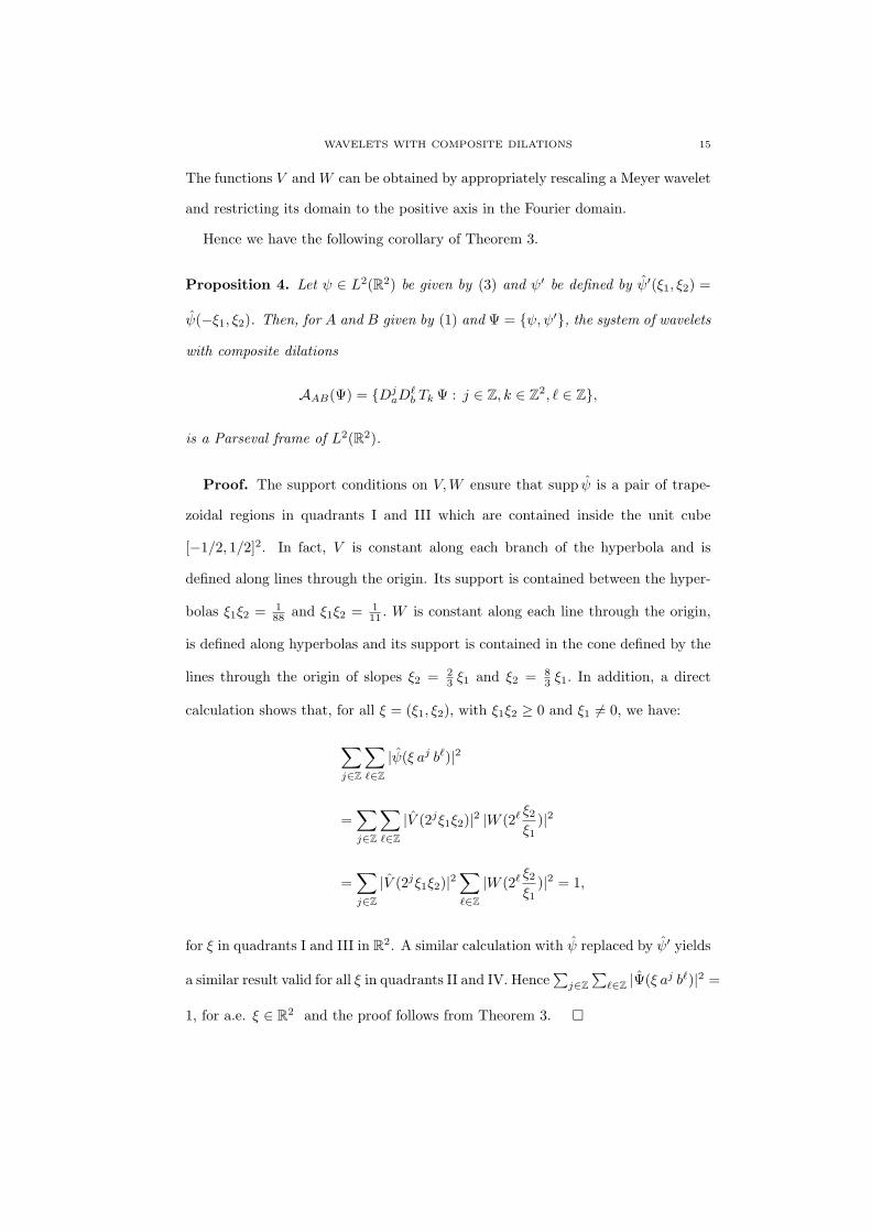
An argument similar to Proposition 4 shows that it is possible to construct a
similar well-localized Parseval frame by replacing the set of isotropic dilations A
given by (1) with the anisotropic dilations (2).
Figure 6. Tiling of the frequency domain associated with a hy-perbolic system of wavelets with composite dilations.
Note that, for a discrete implementation of the hyperbolic systems, the indices
j and ℓ need to be limited to a finite range. The asymptotic regions not covered
because of this discretization can then be dealt with by partitioning the comple-
mentary regions with a Laplacian Pyramid-type of filtering. A form of the tiling
of the frequency plane associated with this construction is illustrated in Figure 6.
For the correct interpretations of this figure, observe that the elements of the well-
localized system of wavelets with composite dilations ψ(ajbℓx) do overlap in the
frequency domain. That is, Figure 6 should be interpreted as a picture of the essen-
tial frequency support (i.e., the regions where most of the norm is concentrated),
rather than the exact frequency support of the elements of the system.
2.2.2. Cone-based hyperbolic construction. The hyperbolic construction suffers from
a bias in directional sensitivity along the orientations ±π/4,±3π/4. In addition,
the regions along the orthogonal axes in the frequency domain are only covered
asymptotically, for values ℓ → ±∞. To overcome this situation, we define the
WAVELETS WITH COMPOSITE DILATIONS 17
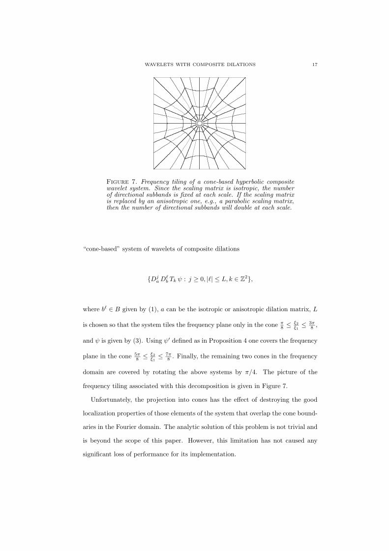
Figure 7. Frequency tiling of a cone-based hyperbolic compositewavelet system. Since the scaling matrix is isotropic, the numberof directional subbands is fixed at each scale. If the scaling matrixis replaced by an anisotropic one, e.g., a parabolic scaling matrix,then the number of directional subbands will double at each scale.
“cone-based” system of wavelets of composite dilations
{DjaD
ℓb Tk ψ : j ≥ 0, |ℓ| ≤ L, k ∈ Z2},
where bℓ ∈ B given by (1), a can be the isotropic or anisotropic dilation matrix, L
is chosen so that the system tiles the frequency plane only in the cone π8 ≤ ξ2
ξ1≤ 3π
8 ,
and ψ is given by (3). Using ψ′ defined as in Proposition 4 one covers the frequency
plane in the cone 5π8 ≤ ξ2
ξ1≤ 7π
8 . Finally, the remaining two cones in the frequency
domain are covered by rotating the above systems by π/4. The picture of the
frequency tiling associated with this decomposition is given in Figure 7.
Unfortunately, the projection into cones has the effect of destroying the good
localization properties of those elements of the system that overlap the cone bound-
aries in the Fourier domain. The analytic solution of this problem is not trivial and
is beyond the scope of this paper. However, this limitation has not caused any
significant loss of performance for its implementation.
18 GLENN R. EASLEY, DEMETRIO LABATE, VISHAL M. PATEL
3. Composite Wavelet Implementation
3.1. Analysis Filter Design. In this section, we describe a novel approach for the
construction of filters that match the frequency tiling associated with the desired
system of wavelets with composite dilations. Given a system of wavelets with
composite dilations AAB(Ψ), this approach allows us to directly apply the set of
matrices A and B to generate the specific frequency tiling associated with the
system AAB(Ψ).
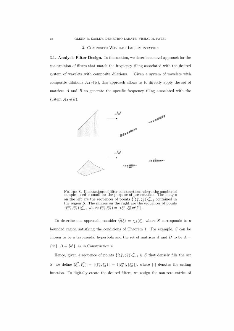
-ajbℓ
-ajbℓ
Figure 8. Illustrations of filter constructions where the number ofsamples used is small for the purpose of presentation. The imageson the left are the sequences of points {(ξn1 , ξn2 )}Nn=1 contained inthe region S. The images on the right are the sequences of points{(ηn1 , ηn2 )}Nn=1 where (ηn1 , η
n2 ) = ⌈(ξn1 , ξn2 )ajbℓ⌉.
To describe our approach, consider ψ(ξ) = χS(ξ), where S corresponds to a
bounded region satisfying the conditions of Theorem 1. For example, S can be
chosen to be a trapezoidal hyperbola and the set of matrices A and B to be A =
{aj}, B = {bℓ}, as in Construction 4.
Hence, given a sequence of points {(ξn1 , ξn2 )}Nn=1 ∈ S that densely fills the set
S, we define (ξn
1 , ξn
2 ) = ⌈(ξn1 , ξn2 )⌉ = (⌈ξn1 ⌉, ⌈ξn2 ⌉), where ⌈·⌉ denotes the ceiling
function. To digitally create the desired filters, we assign the non-zero entries of

WAVELETS WITH COMPOSITE DILATIONS 19
Figure 9. Examples of hyperbolic filters. From left to right: TimeDomain, Frequency Domain
our starting filter G0,0 by the evaluation G0,0(ξn
1 , ξn
2 ) = 1. We then proceed to
create the other filters {Gi,ℓ} by assigning the non-zeros entries as Gi,ℓ(ηn1 , η
n2 ) = 1
for (ηn1 , ηn2 ) = ⌈(ξn1 , ξn2 ) ajbℓ⌉. Note that N needs to be chosen large enough so that
the points (ηn1 , ηn2 ) are dense enough to fill out the regions Sj,ℓ = Sajbℓ completely
in terms of its pixelated image for all desired values of j and ℓ. Thus, the density
is relative to the size of the pixelated image grid. An example of such an N is
provided in the appendix. Figure 8 illustrates this construction.
This construction can be modified to create the well-localized version of wavelets
of composite dilations by the following modification. We start by creating an ini-
tial densely supported filter with the desired windowing. By keeping track of the
multiple assigned grid points, the windowing can be appropriately compensated by
assigning the average windowed value at these point locations. Examples of this
construction are shown in Figure 9 and a pseudo-code for creating such filters is
given in the Appendix. This construction process can be applied to any planar
20 GLENN R. EASLEY, DEMETRIO LABATE, VISHAL M. PATEL
region and can be viewed as a refinement of the original discrete shearlet transform
construction given in [17]. In fact, when the techniques suggested in this paper
are used to design filters for a revised discrete shearlet transform, the newly con-
structed discrete transform performs significantly better than its first incarnation.
Recall that the original shearlet implementation was based on the use of a map-
ping function that performed a re-arrangement of windowed data in a pseudo-polar
grid onto a Cartesian grid. In our new implementation, we avoid the use of the
mapping function and are able to produce the appropriate windowed data directly
onto the Cartesian grid. In addition, this implementation is multi-channel, so that
the estimates provided from individual filtered coefficients are not level-dependent
and this improves the transform’s conditioning. In contrast with [17], where an
inverse mapping function was used to take care of weighting the multiple assigned
pixel values, by avoiding the re-mapping process, we can now avoid creating re-
arrangement domains (a process which usually generated some artifacts). In fact,
we are able to obtain the desired filters by directly applying the A and B dila-
tions associated with the desired composite wavelet decompositions. This way, the
discrete implementation provides a perfect match with its theoretical counterpart
and it allows one to deal even with very complicated geometrical decompositions
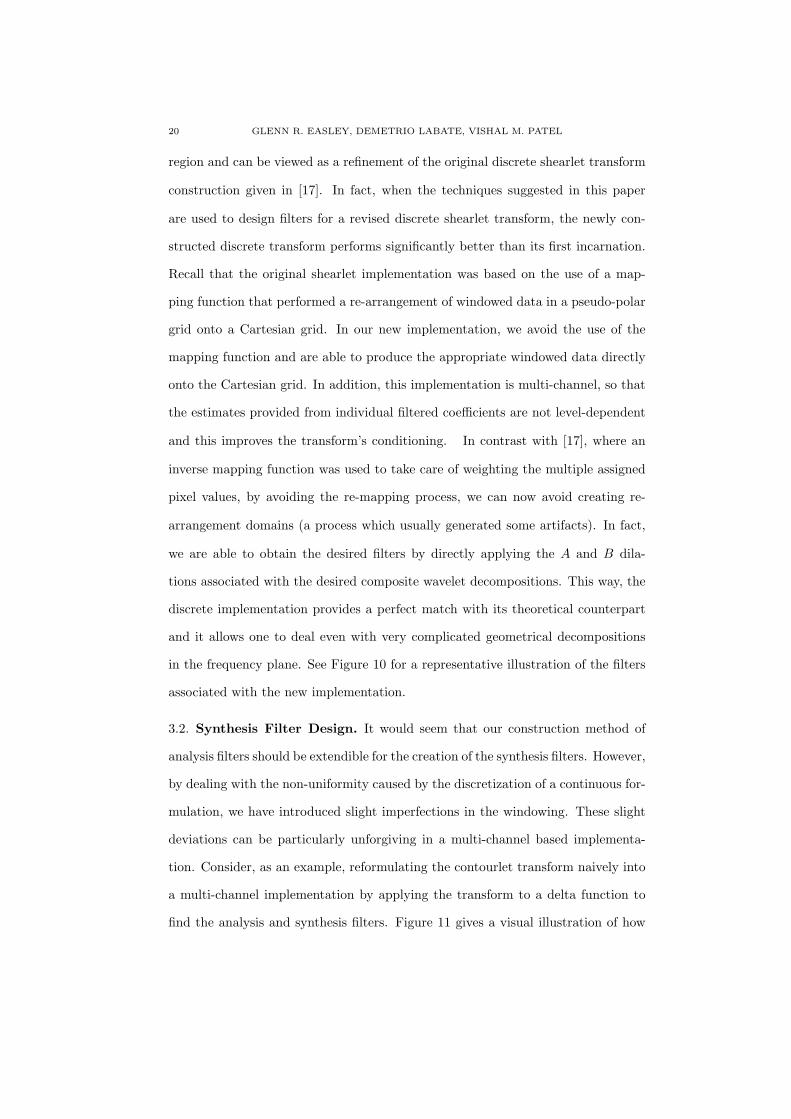
in the frequency plane. See Figure 10 for a representative illustration of the filters
associated with the new implementation.
3.2. Synthesis Filter Design. It would seem that our construction method of
analysis filters should be extendible for the creation of the synthesis filters. However,
by dealing with the non-uniformity caused by the discretization of a continuous for-
mulation, we have introduced slight imperfections in the windowing. These slight
deviations can be particularly unforgiving in a multi-channel based implementa-
tion. Consider, as an example, reformulating the contourlet transform naively into
a multi-channel implementation by applying the transform to a delta function to
find the analysis and synthesis filters. Figure 11 gives a visual illustration of how
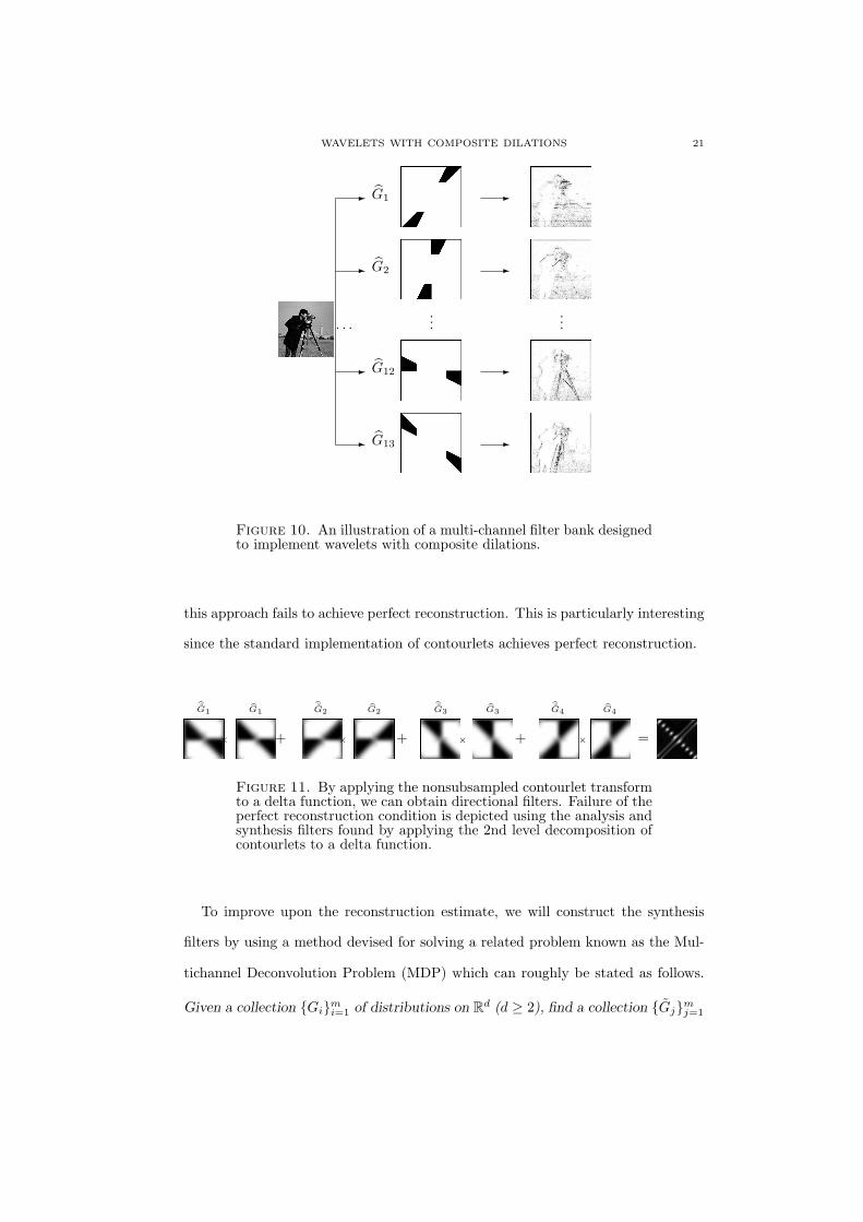
WAVELETS WITH COMPOSITE DILATIONS 21
G1- -
G2- -
.... . .
-G12-
G13- -
...
Figure 10. An illustration of a multi-channel filter bank designedto implement wavelets with composite dilations.
this approach fails to achieve perfect reconstruction. This is particularly interesting
since the standard implementation of contourlets achieves perfect reconstruction.
× =+×+×+×
G1 G1G2 G2
G3 G3G4 G4
Figure 11. By applying the nonsubsampled contourlet transformto a delta function, we can obtain directional filters. Failure of theperfect reconstruction condition is depicted using the analysis andsynthesis filters found by applying the 2nd level decomposition ofcontourlets to a delta function.
To improve upon the reconstruction estimate, we will construct the synthesis
filters by using a method devised for solving a related problem known as the Mul-
tichannel Deconvolution Problem (MDP) which can roughly be stated as follows.
Given a collection {Gi}mi=1 of distributions on Rd (d ≥ 2), find a collection {Gj}mj=1
22 GLENN R. EASLEY, DEMETRIO LABATE, VISHAL M. PATEL
of distributions such that
m∑j=1
Gj ∗Gj = δ,
where δ is a Dirac delta distribution. In the Fourier-Laplace domain, when the
distributions are assumed to be compactly supported, this equation is referred to
as the analytic Bezout equation. This problem has a connection with the polynomial
Bezout equation which is usually solved for computing the filters associated with
traditional filter banks (see [11] for more details).
Several methods for solving the MDP in a discrete setting provide a way of
constructing appropriate synthesis filters (see [39, 40, 2, 3, 29, 18, 11, 48] for details
on some of these methods). One of the earliest and simplest methods for solving
this problem was given in [39]. To explain its derivation, we formulate the problem
in the Fourier domain as follows. Suppose we wish to recover the image f and that
we are given m blurred images sj , i.e.
sj(ξ1, ξ2) = f(ξ1, ξ2) Gj(ξ1, ξ2) + nj for j = 1, . . . ,m,
where Gj and nj are the respective transfer function and associated noise from the
j-th imaging sensor. Assuming that no statistical information is available, find the
image fa which yields a least squares fit between predicted and observed images,
i.e., minimize
m∑j=1
|sj(ξ1, ξ2)− fa(ξ1, ξ2) Gj(ξ1, ξ2)|2.
After differentiating with respect to fa, the solution is found to be
fa(ξ1, ξ2) =
m∑j=1
sj(ξ1, ξ2)Gj(ξ1, ξ2),
WAVELETS WITH COMPOSITE DILATIONS 23
where
Gj(ξ1, ξ2) =Gj(ξ1, ξ2)∑m
k=1 |Gk(ξ1, ξ2)|2,
for j = 1, . . . ,m. The synthesis filters {Gj}mj=1 are robust (and even optimal) with
respect to any residual noise left from the decompositions that might remain after
thresholding schemes have been utilized for denoising purposes. When filters of
small finite support are desired, we use the method given in [11], which reduces the
problem of finding the synthesis filters to solving a constrained matrix inversion
problem. This method is particularly flexible as the support sizes of the synthesis
filters can be controlled by a free parameter that balances between local and global
conditioning.
Another solution to achieve perfect reconstruction is to slightly modify the anal-
ysis filters to be
(4) G′j(ξ1, ξ2) =
Gj(ξ1, ξ2)√∑mk=1 |Gk(ξ1, ξ2)|2
,
and to use
(5) Gj(ξ1, ξ2) =Gj(ξ1, ξ2)√∑mk=1 |Gk(ξ1, ξ2)|2
,
as the synthesis filters for j = 0, . . . ,m− 1. Note that this solution means that the
implemented transform corresponds to a tight frame. However, we have found that
for some constructions the MDP solutions perform better.
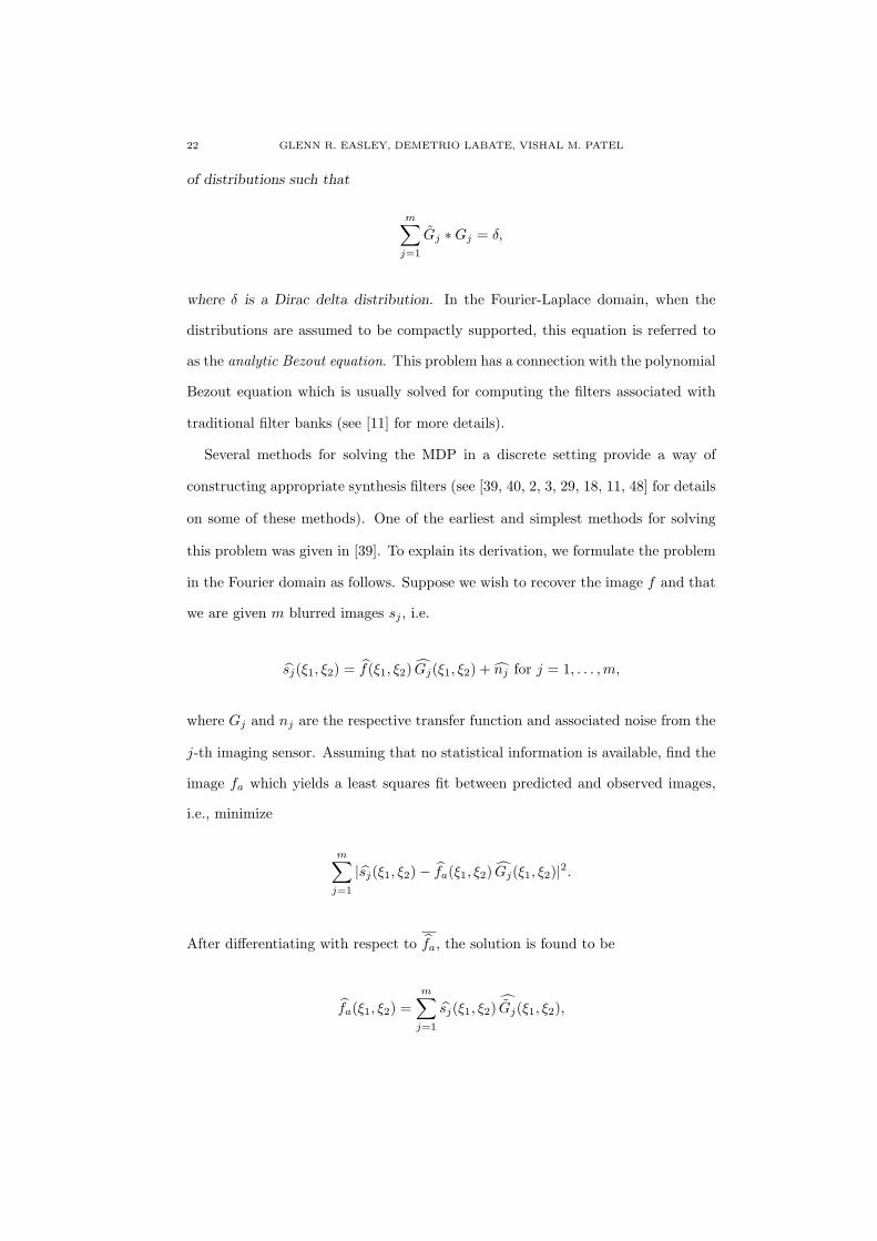
To emphasize the benefits of our proposed filter constructions, we show the differ-
ences in frequency responses for some representatives of the new shearlet filters and
the non-subsampled contourlet transform (NSCT) filters in Figure 12. This illustra-
tion shows that whereas the NSCT filters may be constructed by using conventional
filter design elements, their desired frequency responses do not truly match with
24 GLENN R. EASLEY, DEMETRIO LABATE, VISHAL M. PATEL
Figure 12. Comparison of filters design methods. The imageson the top correspond to examples of the frequency responses ofthe newly constructed shearlet filters. The images on the bottomcorrespond to examples of the frequency responses of the NSCTfor the same directional components.
the actual frequency responses. Nonetheless, the NSCT filters are very effective
and have other advantages.
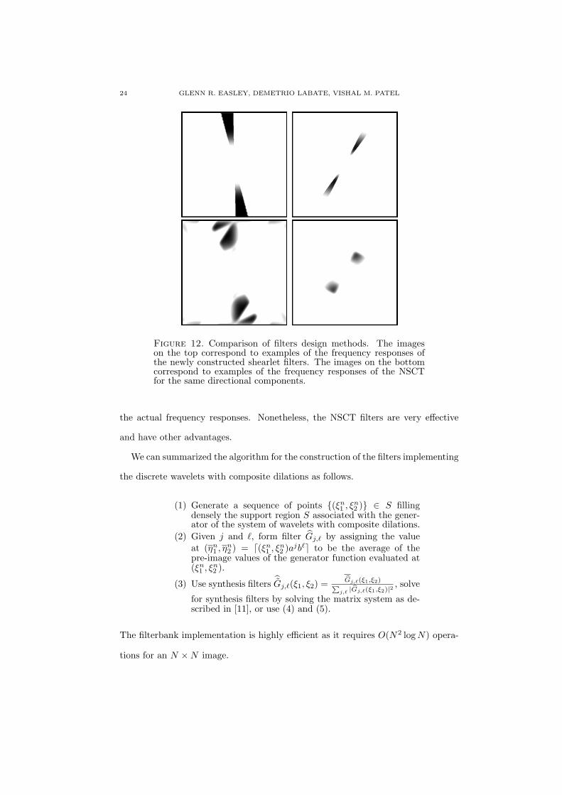
We can summarized the algorithm for the construction of the filters implementing
the discrete wavelets with composite dilations as follows.
(1) Generate a sequence of points {(ξn1 , ξn2 )} ∈ S fillingdensely the support region S associated with the gener-ator of the system of wavelets with composite dilations.
(2) Given j and ℓ, form filter Gj,ℓ by assigning the valueat (ηn1 , η
n2 ) = ⌈(ξn1 , ξn2 )ajbℓ⌉ to be the average of the
pre-image values of the generator function evaluated at(ξn1 , ξ
n2 ).
(3) Use synthesis filters Gj,ℓ(ξ1, ξ2) =Gj,ℓ(ξ1,ξ2)∑
j,ℓ |Gj,ℓ(ξ1,ξ2)|2, solve
for synthesis filters by solving the matrix system as de-scribed in [11], or use (4) and (5).
The filterbank implementation is highly efficient as it requires O(N2 logN) opera-
tions for an N ×N image.
WAVELETS WITH COMPOSITE DILATIONS 25
4. Numerical Experiments
In this section, we present several numerical experiments on image restoration
and enhancement to demonstrate the effectiveness of the wavelets with compos-
ite dilations and their discrete implementation. The simulations were done using
Matlab on a Windows system with Intel Pentium M/1.73 GHz processor.
4.1. Denoising. In the first set of experiments, we illustrate the denoising capa-
bility of the new wavelets with composite dilations by means of hard thresholding.
The objective of this problem is to recover an image x, given noisy observations
y = x+ γ,
where γ is zero-mean white Gaussian noise with variance σ2. By adapting the
standard wavelet shrinkage approach [37], we apply a hard threshold on the subband
coefficients of several versions of composite wavelets decompositions. In particular,
we choose the threshold Tj = Kσj , where σ2j is the noise variance in each subband
and K is a constant. In our experiments, we set K = 2 for all subbands.
To assess the denoising performance of our method, we compare it against three
different competing discrete multiscale transforms: the nonsubsampled wavelet
transform (NSWT), the second generation curvelet transform (curv) [7], and the
nonsubsampled contourlet transform (NSCT). The discrete wavelets with compos-
ite dilations we have tested are the new shearlet transform (ab-shear), the cone-
based hyperbolic transform (c-hyper), the hyperbolic transform (hyper), the star-
like transform given in Construction 1 (ab-star). Specifically, the new constructions
are done using the pseudo-code shown in the appendix so that the frequency plane
decompositions correspond to the decompositions displayed in Figures 2 (left side),
3, 6, and 8. The value of N0 is set to the size of the image the transform is being
applied to. For the sake of comparison, we have also included the original imple-
mentation of the shearlet transform (shear) [17]. The peak signal-to-noise ratio
26 GLENN R. EASLEY, DEMETRIO LABATE, VISHAL M. PATEL
(PSNR) is used to measure the performance of the different transforms. Given an
N ×N image x and its estimate x, the PSNR in decibels (dB) is defined as
PSNR = 20 log10255N
∥x− x∥F,
where ∥.∥F is the Frobenius norm. In Tables I and II, we show the results obtained
using various discrete transforms on the Peppers and Barbara images, respectively.
The highest PSNR for each experiment is shown in bold. As it can be seen from
the tables, all our new transforms provide superior or comparable results to that
obtained using NSWT, NSCT and curvelets. Indeed, in some cases, the composite
wavelet transforms provide improvement of nearly 1 dB or more compared to the
competing algorithms. Figures 13, 14, 15 and 16 show some of the reconstructed
images for these various experiments.
Table I: Denoising results using Peppers image.
σ Noisy ab-shear c-hyper hyper ab-star NSWT shear NSCT curv
10 28.17 34.28 33.70 33.91 33.45 33.71 34.05 33.81 32.3620 22.15 31.82 31.01 31.28 30.83 31.19 31.78 31.60 29.6530 18.63 30.25 29.35 29.72 29.26 29.43 30.13 30.07 28.2540 16.13 29.01 28.12 28.40 28.04 28.09 28.86 28.85 27.2850 14.20 27.98 27.17 27.33 26.99 27.04 27.90 27.82 26.46
Table II: Denoising results using Barbara image.
σ Noisy ab-shear c-hyper hyper ab-star NSWT shear NSCT curv
10 28.17 33.47 33.97 33.81 32.29 31.58 33.12 33.01 29.1620 22.15 30.38 30.41 30.49 29.02 27.23 30.07 29.41 25.4630 18.63 28.44 28.37 28.53 27.02 25.10 28.16 27.24 24.4240 16.14 26.93 26.86 26.75 25.55 24.02 26.59 25.79 23.8150 14.20 25.59 25.78 25.35 24.06 23.37 25.39 24.79 23.33
In Table III, we report average runtime of the different transforms in filtering
noisy images. Note that NSWT and curv use preconstructed filters. As a result
they are very fast and run in less than a minute. The performance of our composite
wavelet transforms can be significantly enhanced by implementing them in a parallel
form and using other modifications, but this is beyond the scope of this paper.
WAVELETS WITH COMPOSITE DILATIONS 27
(a) (b)
(c) (d)
(e) (f)
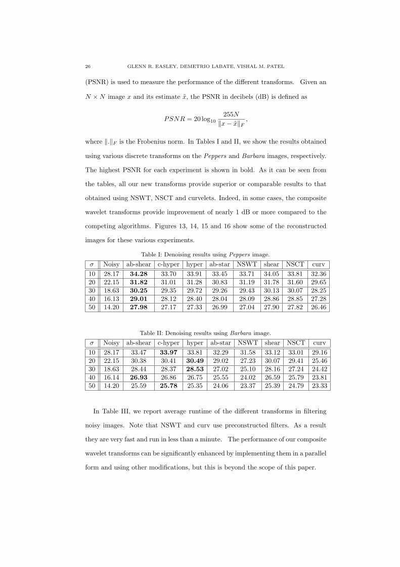
Figure 13. Denoising experiments with a Barbara image. (a)Original image. (b) Noisy image with σ = 20, PSNR=22.15 dB.(c) Restored image using ab-shear, PSNR=30.38 dB . (d) Re-stored image using c-hyper, PSNR=30.41 dB. (e) Restored imageusing hyper, PSNR=30.49 dB. (f) Restored image using ab-star,PSNR=29.02 dB.
28 GLENN R. EASLEY, DEMETRIO LABATE, VISHAL M. PATEL
(a) (b)
(c) (d)
(e) (f)
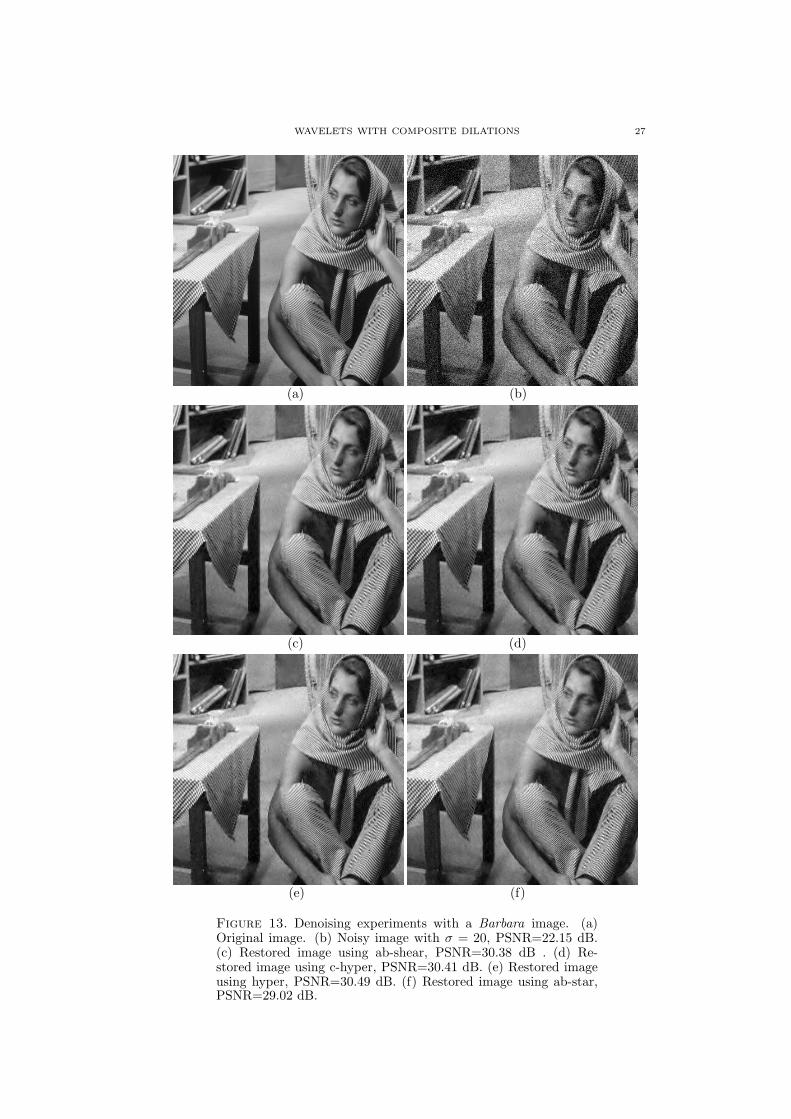
Figure 14. Denoising experiments with a Barbara image. (a)Original image. (b) Noisy image with σ = 50, PSNR=14.20 dB.(c) Restored image using ab-shear, PSNR=25.59 dB . (d) Re-stored image using c-hyper, PSNR=25.78 dB. (e) Restored imageusing hyper, PSNR=25.35 dB. (f) Restored image using ab-star,PSNR=24.06 dB.
WAVELETS WITH COMPOSITE DILATIONS 29
(a) (b)
(c) (d)
(e) (f)
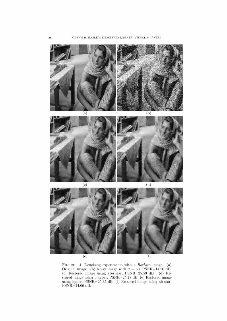
Figure 15. Denoising experiments with a Peppers image. (a)Original image. (b) Noisy image with σ = 20, PSNR=22.15 dB.(c) Restored image using ab-shear, PSNR=31.82 dB . (d) Re-stored image using c-hyper, PSNR=31.01 dB. (e) Restored imageusing hyper, PSNR=31.28 dB. (f) Restored image using ab-star,PSNR=30.83 dB.

30 GLENN R. EASLEY, DEMETRIO LABATE, VISHAL M. PATEL
(a) (b)
(c) (d)
(e) (f)
Figure 16. Denoising experiments with a Peppers image. (a)Original image. (b) Noisy image with σ = 50, PSNR=14.20 dB.(c) Restored image using ab-shear, PSNR=27.98 dB . (d) Re-stored image using c-hyper, PSNR=27.17 dB. (e) Restored imageusing hyper, PSNR=27.33 dB. (f) Restored image using ab-star,PSNR=26.99 dB.
WAVELETS WITH COMPOSITE DILATIONS 31
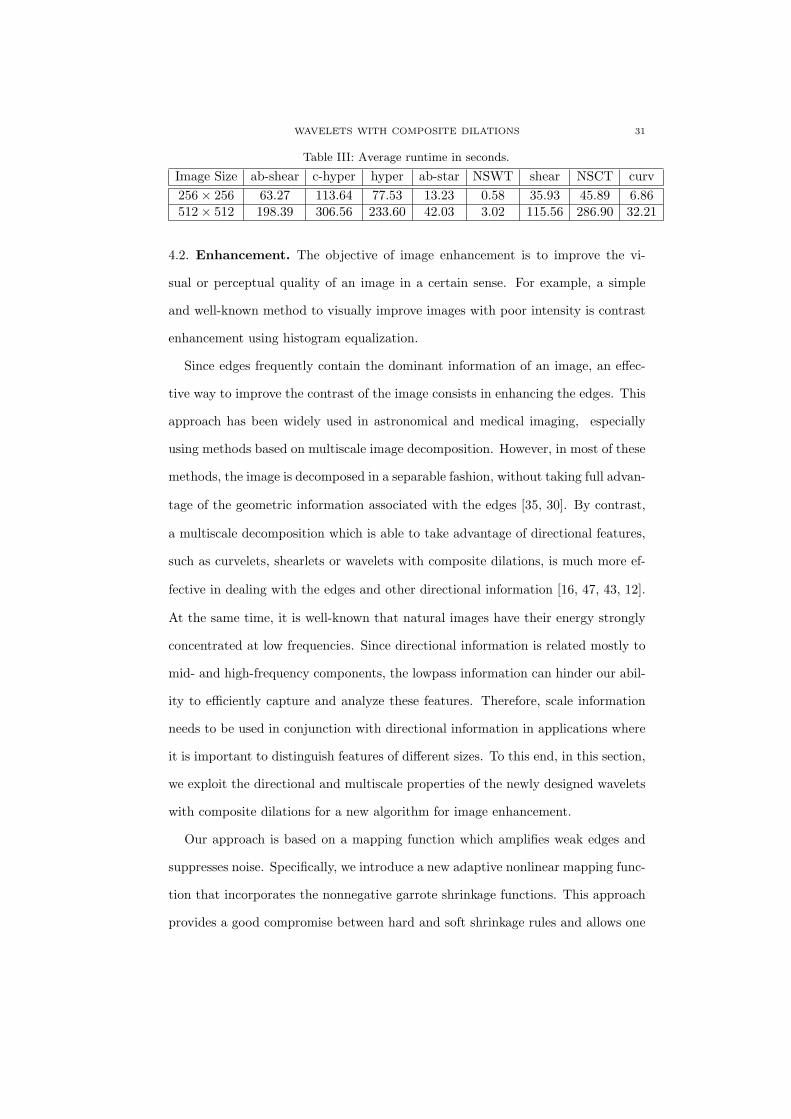
Table III: Average runtime in seconds.
Image Size ab-shear c-hyper hyper ab-star NSWT shear NSCT curv
256× 256 63.27 113.64 77.53 13.23 0.58 35.93 45.89 6.86512× 512 198.39 306.56 233.60 42.03 3.02 115.56 286.90 32.21
4.2. Enhancement. The objective of image enhancement is to improve the vi-
sual or perceptual quality of an image in a certain sense. For example, a simple
and well-known method to visually improve images with poor intensity is contrast
enhancement using histogram equalization.
Since edges frequently contain the dominant information of an image, an effec-
tive way to improve the contrast of the image consists in enhancing the edges. This
approach has been widely used in astronomical and medical imaging, especially
using methods based on multiscale image decomposition. However, in most of these
methods, the image is decomposed in a separable fashion, without taking full advan-
tage of the geometric information associated with the edges [35, 30]. By contrast,
a multiscale decomposition which is able to take advantage of directional features,
such as curvelets, shearlets or wavelets with composite dilations, is much more ef-
fective in dealing with the edges and other directional information [16, 47, 43, 12].
At the same time, it is well-known that natural images have their energy strongly
concentrated at low frequencies. Since directional information is related mostly to
mid- and high-frequency components, the lowpass information can hinder our abil-
ity to efficiently capture and analyze these features. Therefore, scale information
needs to be used in conjunction with directional information in applications where
it is important to distinguish features of different sizes. To this end, in this section,
we exploit the directional and multiscale properties of the newly designed wavelets
with composite dilations for a new algorithm for image enhancement.
Our approach is based on a mapping function which amplifies weak edges and
suppresses noise. Specifically, we introduce a new adaptive nonlinear mapping func-
tion that incorporates the nonnegative garrote shrinkage functions. This approach
provides a good compromise between hard and soft shrinkage rules and allows one
32 GLENN R. EASLEY, DEMETRIO LABATE, VISHAL M. PATEL
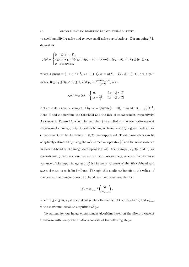
to avoid amplifying noise and remove small noise perturbations. Our mapping f is
defined as
f(y) =
0 if |y| < T1,
sign(y)T2 + α(sigm(c(gy − β))− sigm(−c(gy + β))) if T2 ≤ |y| ≤ T3,
y otherwise.
where sigm(y) = (1 + e−y)−1, y ∈ [−1, 1], α = α(T3 − T2), β ∈ (0, 1), c is a gain
factor, 0 ≤ T1 ≤ T2 < T3 ≤ 1, and gy =garroteT2
(y)
T3−T2, with
garroteT2(y) =
{0, for |y| ≤ T2
y − T 22
y , for |y| > T2
Notice that α can be computed by α = (sigm(c(1 − β)) − sigm(−c(1 + β)))−1.
Here, β and c determine the threshold and the rate of enhancement, respectively.
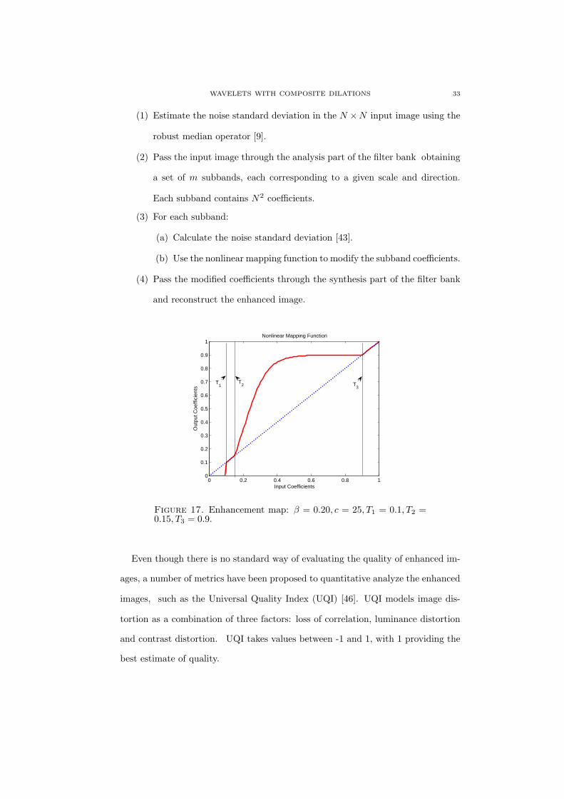
As shown in Figure 17, when the mapping f is applied to the composite wavelet
transform of an image, only the values falling in the interval [T2, T3] are modified for
enhancement, while the values in [0, T1] are suppressed. These parameters can be
adaptively estimated by using the robust median operator [9] and the noise variance
in each subband of the image decomposition [44]. For example, T1, T2, and T3 for
the subband j can be chosen as pσj , qσj , rσj , respectively, where σ2 is the noise
variance of the input image and σ2j is the noise variance of the jth subband and
p, q and r are user defined values. Through this nonlinear function, the values of
the transformed image in each subband are pointwise modified by
yk = ykmaxf
(ykykmax
),
where 1 ≤ k ≤ m, yk is the output of the kth channel of the filter bank, and ykmax
is the maximum absolute amplitude of yk.
To summarize, our image enhancement algorithm based on the discrete wavelet
transform with composite dilations consists of the following steps:
WAVELETS WITH COMPOSITE DILATIONS 33
(1) Estimate the noise standard deviation in the N ×N input image using the
robust median operator [9].
(2) Pass the input image through the analysis part of the filter bank obtaining
a set of m subbands, each corresponding to a given scale and direction.
Each subband contains N2 coefficients.
(3) For each subband:
(a) Calculate the noise standard deviation [43].
(b) Use the nonlinear mapping function to modify the subband coefficients.
(4) Pass the modified coefficients through the synthesis part of the filter bank
and reconstruct the enhanced image.
0 0.2 0.4 0.6 0.8 10
0.1
0.2
0.3
0.4
0.5
0.6
0.7
0.8
0.9
1Nonlinear Mapping Function
Input Coefficients
Out
put C
oeffi
cien
ts
T1
T2 T
3
Figure 17. Enhancement map: β = 0.20, c = 25, T1 = 0.1, T2 =0.15, T3 = 0.9.
Even though there is no standard way of evaluating the quality of enhanced im-
ages, a number of metrics have been proposed to quantitative analyze the enhanced
images, such as the Universal Quality Index (UQI) [46]. UQI models image dis-
tortion as a combination of three factors: loss of correlation, luminance distortion
and contrast distortion. UQI takes values between -1 and 1, with 1 providing the
best estimate of quality.
34 GLENN R. EASLEY, DEMETRIO LABATE, VISHAL M. PATEL
(a) (b)
(c) (d)
(e) (f)
Figure 18. Enhancement experiments with a Barbara image. (a)Original image. (b) Enhanced using NSWT. (c) Enhanced usingab-shear. (d) Enhanced using hyper. (e) Enhanced using c-hyper.(f) Enhanced using ab-star.
WAVELETS WITH COMPOSITE DILATIONS 35
(a) (b)
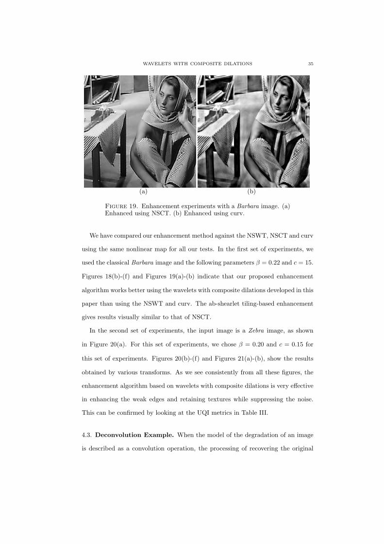
Figure 19. Enhancement experiments with a Barbara image. (a)Enhanced using NSCT. (b) Enhanced using curv.
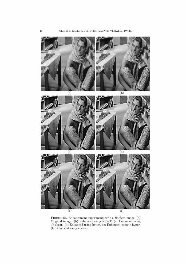
We have compared our enhancement method against the NSWT, NSCT and curv
using the same nonlinear map for all our tests. In the first set of experiments, we
used the classical Barbara image and the following parameters β = 0.22 and c = 15.
Figures 18(b)-(f) and Figures 19(a)-(b) indicate that our proposed enhancement
algorithm works better using the wavelets with composite dilations developed in this
paper than using the NSWT and curv. The ab-shearlet tiling-based enhancement
gives results visually similar to that of NSCT.
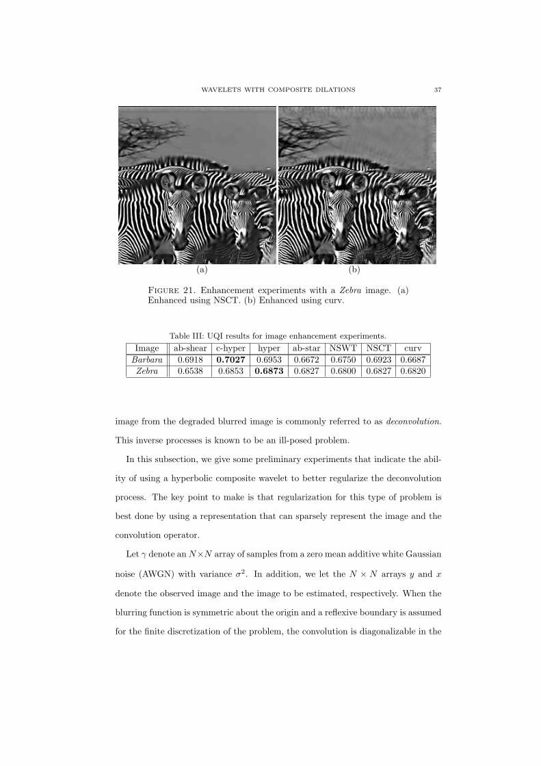
In the second set of experiments, the input image is a Zebra image, as shown
in Figure 20(a). For this set of experiments, we chose β = 0.20 and c = 0.15 for
this set of experiments. Figures 20(b)-(f) and Figures 21(a)-(b), show the results
obtained by various transforms. As we see consistently from all these figures, the
enhancement algorithm based on wavelets with composite dilations is very effective
in enhancing the weak edges and retaining textures while suppressing the noise.
This can be confirmed by looking at the UQI metrics in Table III.
4.3. Deconvolution Example. When the model of the degradation of an image
is described as a convolution operation, the processing of recovering the original

36 GLENN R. EASLEY, DEMETRIO LABATE, VISHAL M. PATEL
(a) (b)
(c) (d)
(e) (f)
Figure 20. Enhancement experiments with a Zebra image. (a)Original image. (b) Enhanced using NSWT. (c) Enhanced usingab-shear. (d) Enhanced using hyper. (e) Enhanced using c-hyper.(f) Enhanced using ab-star.
WAVELETS WITH COMPOSITE DILATIONS 37
(a) (b)
Figure 21. Enhancement experiments with a Zebra image. (a)Enhanced using NSCT. (b) Enhanced using curv.
Table III: UQI results for image enhancement experiments.
Image ab-shear c-hyper hyper ab-star NSWT NSCT curv
Barbara 0.6918 0.7027 0.6953 0.6672 0.6750 0.6923 0.6687Zebra 0.6538 0.6853 0.6873 0.6827 0.6800 0.6827 0.6820
image from the degraded blurred image is commonly referred to as deconvolution.
This inverse processes is known to be an ill-posed problem.
In this subsection, we give some preliminary experiments that indicate the abil-
ity of using a hyperbolic composite wavelet to better regularize the deconvolution
process. The key point to make is that regularization for this type of problem is
best done by using a representation that can sparsely represent the image and the
convolution operator.
Let γ denote anN×N array of samples from a zero mean additive white Gaussian
noise (AWGN) with variance σ2. In addition, we let the N × N arrays y and x
denote the observed image and the image to be estimated, respectively. When the
blurring function is symmetric about the origin and a reflexive boundary is assumed
for the finite discretization of the problem, the convolution is diagonalizable in the
38 GLENN R. EASLEY, DEMETRIO LABATE, VISHAL M. PATEL
DCT domain. Thus we write the deconvolution problem in the DCT domain as
(6) Y (k1, k2) = H(k1, k2)X(k1, k2) + Γ(k1, k2),
where Y (k1, k2),H(k1, k2), X(k1, k2) and Γ(k1, k2) are the 2D DCTs of y, h, x, and
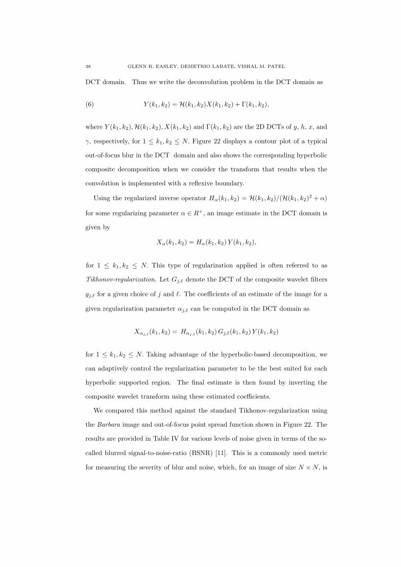
γ, respectively, for 1 ≤ k1, k2 ≤ N. Figure 22 displays a contour plot of a typical
out-of-focus blur in the DCT domain and also shows the corresponding hyperbolic
composite decomposition when we consider the transform that results when the
convolution is implemented with a reflexive boundary.
Using the regularized inverse operator Hα(k1, k2) = H(k1, k2)/(H(k1, k2)2 + α)
for some regularizing parameter α ∈ R+, an image estimate in the DCT domain is
given by
Xα(k1, k2) = Hα(k1, k2)Y (k1, k2),
for 1 ≤ k1, k2 ≤ N. This type of regularization applied is often referred to as
Tikhonov-regularization. Let Gj,ℓ denote the DCT of the composite wavelet filters
gj,ℓ for a given choice of j and ℓ. The coefficients of an estimate of the image for a
given regularization parameter αj,ℓ can be computed in the DCT domain as
Xαj,ℓ(k1, k2) = Hαj,ℓ
(k1, k2)Gj,ℓ(k1, k2)Y (k1, k2)
for 1 ≤ k1, k2 ≤ N. Taking advantage of the hyperbolic-based decomposition, we
can adaptively control the regularization parameter to be the best suited for each
hyperbolic supported region. The final estimate is then found by inverting the
composite wavelet transform using these estimated coefficients.
We compared this method against the standard Tikhonov-regularization using
the Barbara image and out-of-focus point spread function shown in Figure 22. The
results are provided in Table IV for various levels of noise given in terms of the so-
called blurred signal-to-noise-ratio (BSNR) [11]. This is a commonly used metric
for measuring the severity of blur and noise, which, for an image of size N ×N , is
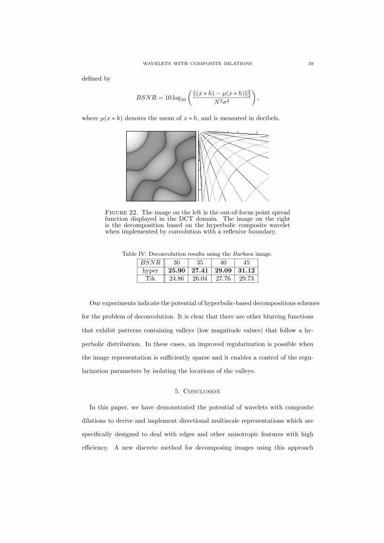
WAVELETS WITH COMPOSITE DILATIONS 39
defined by
BSNR = 10 log10
(∥(x ∗ h)− µ(x ∗ h)∥22
N2σ2
),
where µ(x ∗ h) denotes the mean of x ∗ h, and is measured in decibels.
Figure 22. The image on the left is the out-of-focus point spreadfunction displayed in the DCT domain. The image on the rightis the decomposition based on the hyperbolic composite waveletwhen implemented by convolution with a reflexive boundary.
Table IV: Deconvolution results using the Barbara image.
BSNR 30 35 40 45hyper 25.90 27.41 29.09 31.12Tik 24.86 26.04 27.76 29.73
Our experiments indicate the potential of hyperbolic-based decompositions schemes
for the problem of deconvolution. It is clear that there are other blurring functions
that exhibit patterns containing valleys (low magnitude values) that follow a hy-
perbolic distribution. In these cases, an improved regularization is possible when
the image representation is sufficiently sparse and it enables a control of the regu-
larization parameters by isolating the locations of the valleys.
5. Conclusion
In this paper, we have demonstrated the potential of wavelets with composite
dilations to derive and implement directional multiscale representations which are
specifically designed to deal with edges and other anisotropic features with high
efficiency. A new discrete method for decomposing images using this approach
40 GLENN R. EASLEY, DEMETRIO LABATE, VISHAL M. PATEL
was devised which follows directly from the generating structure and is much more
flexible and sophisticated than previous design concepts. In fact, this new method
is able to produce very sophisticate geometrical decompositions of the frequency
plane such as the new hyperbolic decomposition. Our new discrete transforms even
improve upon the original implementation of the discrete shearlet transform, whose
advantages in denoising and other imaging applications have been established in
previous works. The numerical demonstrations included in this paper show that
our new discrete transforms perform consistently better than similar directional
multiscale transforms in problems of image denoising and enhancement.
Acknowledgments. D.L. acknowledges partial support from NSF grants DMS
1008900 and DMS 1005799 and NHARP grant 003652-0136-2009.
References
[1] R. H. Bamberger and M. J. T. Smith, A filter bank for directional decomposition of images:
theory and design, IEEE Trans. Signal Process., 40(2), pp. 882–893, 1992.
[2] C. A. Berenstein, A. Yger, and B. A. Taylor, Sur quelques formules explicites de deconvolu-
tion, Journal of Optics (Paris), 14, pp. 75–82, 1983.
[3] C. A. Berenstein, and A. Yger, Le probleme de la deconvolution, J. Funct. Anal., pp. 113–160,
1983.
[4] J. D. Blanchard, Minimally supported frequency composite dilation wavelets, J. Fourier Anal.
Appl., 15, pp. 796–815, 2009.
[5] J. D. Blanchard, Minimally Supported Frequency Composite Dilation Parseval Frame
Wavelets, J. Geom. Anal., 19, pp. 19–35, 2009.
[6] J. D. Blanchard and I. A. Krishtal, Matricial filters and crystallographic composite dilation
wavelets, Math. Comp., 81 pp. 905–922, 2012.
[7] E. J. Candes, L. Demanet, D. L. Donoho and L. Ying. Fast discrete curvelet transforms,
Multiscale Model. Simul., 5, pp. 861–899, 2006.
WAVELETS WITH COMPOSITE DILATIONS 41
[8] E. J. Candes and D. L. Donoho, New tight frames of curvelets and optimal representations
of objects with piecewise C2 singularities, Comm. Pure and Appl. Math., 56, pp. 216–266,
2004.
[9] S. G. Chang, B. Yu, and M. Vetterli, Spatially adaptive wavelet thresholding with context
modeling for image denoising, IEEE Trans. on Imag. Processing, 9(9), pp. 1522-1531, 2000.
[10] J. Chung, G. R. Easley, and D. P. O’Leary, Windowed Spectral Regularization of Inverse
Problems, SIAM J. Sci. Comput., 33(6), pp. 3175-3200, 2012.
[11] F. Colonna, and G. R. Easley, The multichannel deconvolution problem: a discrete analysis,
J. Fourier Anal. Appl. 10, pp. 351–376, 2004.
[12] A. L. Cunha, J. Zhou, M. N. Do, The nonsubsampled contourlet transform: Theory, design,
and applications, IEEE Trans. Image Processing, 15, pp. 3089–3101, 2006.
[13] M. N. Do and M. Vetterli, The contourlet transform: an efficient directional multiresolution
image representation, IEEE Trans. Image Process., 14(12), pp. 2091–2106, 2005.
[14] S. Durand, Orthonormal bases of non-separable wavelets with sharp directions, Proceedings
of IEEE Int. Conf. on Image Proc., 2005.
[15] S. Durand, M-band filtering and non-redundant directional wavelets, Appl. Comput. Harmon.
Anal., 22(1), pp. 124–139, 2007.
[16] G. Easley, D. Labate, Critically sampled wavelets with composite dilations, IEEE Trans.
Image Process., 21(2), pp. 550–561, 2012.
[17] G. Easley, D. Labate and W. Lim, Sparse Directional Image Representations using the Dis-
crete Shearlet Transform, Appl. Comput. Harmon. Anal., 25, pp. 25–46, 2008.
[18] G. R. Easley, and D. F. Walnut, Local multichannel deconvolution, J. Math. Imaging Vision,
18, pp. 69–80, 2003.
[19] K. Egan, Y-T Tseng, N. Holzschuch, F. Durand, R. Ramamorthi, Frequency Analysis and
Sheared Reconstruction for Rendering Motion Blur, ACM Transactions on Graphics, 28(3),
pp. 1–13, 2009.
[20] R. Eslami and H. Radha, New image transforms using hybrid wavelets and directional filter
banks: Analysis and design, Proc. IEEE Int. Conf. Image Process. ICIP2005. Genova, Italy,
2005.
42 GLENN R. EASLEY, DEMETRIO LABATE, VISHAL M. PATEL
[21] R. Eslami and H. Radha, Regular hybrid wavelets and directional filter banks: Extensions
and applications, Proc. IEEE Int. Conf. Image Process. ICIP2006. Atlanta, GA, 2006.
[22] R. Eslami and H. Radha, A new family of nonredundant transforms using hybrid wavelets
and directional filter banks, IEEE Trans. Image Process., 16(4), pp. 1152–1167, 2007.
[23] W. T. Freeman and E. H. Adelson, The design and use of steerable filters, IEEE Trans. Patt.
Anal. Mach. Intell., 9, pp. 891–906, 1991.
[24] K. Guo and D. Labate, Optimally sparse multidimensional representation using shearlets,
SIAM J. Math. Anal., 9, pp. 298–318, 2007.
[25] K. Guo, and D. Labate, Optimally Sparse 3D Approximations using Shearlet Representations,
Electronic Research Announcements in Mathematical Sciences, 17 pp. 126-138, 2010.
[26] K. Guo, D. Labate, W.-Q. Lim, D. Labate, G. Weiss, and E. Wilson, Wavelets with composite
dilations, Electron. Res. Announc. Amer. Math. Soc., 10, pp. 78–87, 2004.
[27] K. Guo, D. Labate, W.-Q. Lim, D. Labate, G. Weiss, and E. Wilson, Wavelets with composite
dilations and their MRA properties, Appl. Comput. Harmon. Anal., 20, pp. 220–236, 2006.
[28] K. Guo, D. Labate, W.-Q. Lim, D. Labate, G. Weiss, and E. Wilson, The theory of wavelets
with composite dilations in: Harmonic Analysis and Applications, C. Heil (ed.), pp. 231–249,
Birkhauser, Boston, MA, 2006.
[29] G. Harikumar, and Y. Bresler, FIR perfect signal reconstruction from multiple convolutions:
minimum deconvolver orders, IEEE Trans. Sign. Proc. 46, pp. 215–218, 1998.
[30] J. Lu, D. M. Healy, Jr., Contrast enhancement via multi-scale gradient transformation, in
Wavelet Applications, Proceedings of SPIE, Orlando, FL, April 5-8, 1994.
[31] S. Higaki, S. Kyochi, Y. Tanaka, and M. Ikehara, A novel design of critically sampled con-
tourlet transform and its application to image coding, Proc. IEEE Int. Conf. Image Process.
ICIP2008. San Diego, CA, Oct. 2008.
[32] I. Kryshtal, B. Robinson, G. Weiss, and E. Wilson, Compactly supported wavelets with
composite dilations, J. Geom. Anal. 17, pp. 87–96, 2006.
[33] G. Kutyniok and W. Lim, Compactly supported shearlets are optimally sparse, J. Approx.
Theory, 163, pp. 1564-1589, 2011.
WAVELETS WITH COMPOSITE DILATIONS 43
[34] D. Labate, W. Lim, G. Kutyniok, and G. Weiss, Sparse multidimensional representation
using shearlets, Wavelets XI (San Diego, CA, 2005), pp. 254–262, SPIE Proc., 5914, SPIE,
Bellingham, WA, 2005.
[35] A. F. Laine and X. Zong, A multiscale sub-octave wavelet transform for de-noising and
enhancement, in Wavelet Applications, Proceedings of SPIE, Denver, CO, August 6-9, 1996,
2825, pp. 238-249, 1996.
[36] Y. Lu and M. N. Do, The finer directional wavelet transform, Proceedings of IEEE Inter-
national Conference on Acoustics, Speech, and Signal Processing (ICASSP), Philadelphia,
March 2005.
[37] S. Mallat, A Wavelet Tour of Signal Processing, Academic Press, San Diego, 1998.
[38] T. T. Nguyen and S. Oraintara, Multiresolution direction filterbanks: Theory, design, and
applications, IEEE Trans. Signal Process., 53(10), pp. 3895–3905, 2005.
[39] P. Schiske, Zur frage der bildrekonstruktion durch fokusreihen, Proc. Eur. Reg. Conf. Elec-
tron. Microsc. 4th, pp. 1–145, 1968.
[40] P. Schiske, Image processing using additional statistical information about the object. In
P. W. Hawkes, ed., Image Processing and Computer Aided Design in Electron Optics. Aca-
demic Press, New York, 1973.
[41] E. P. Simoncelli and E. H. Adelson, Non-separable extensions of quadrature mirror filters to
multiple dimensions, Proceedings of the IEEE, 78(4), pp. 652–664, 1990.
[42] J. L. Starck, E. J. Candes, and D. L. Donoho, The curvelet transform for image denoising,
IEEE Trans Image Process., 11(6), pp. 670–684, 2002.
[43] J. L. Starck, F. Murtagh, E. Candes, and D. L. Donoho, Gray and Color Image Contrast
Enhancement by the Curvelet Transform, IEEE Trans. on Imag. Processing, 12(6), pp. 706–
717, 2003.
[44] J. L. Starck, E. J. Candes, and D. L. Donoho, The Curvelet Transform for image denoising,
IEEE Trans. on Imag. Processing, 11(6), pp. 670–684, 2002.
[45] Y. Tanaka, M. Ikehara, and T. Q. Nguyen, Multiresolution image representation using com-
bined 2D and 1D directional filter banks, IEEE Trans. Image Process., 18(2), pp. 269–280,
2009.
44 GLENN R. EASLEY, DEMETRIO LABATE, VISHAL M. PATEL
[46] Z. Wang and A. C. Bovik, A universal image quality index, IEEE Signal Processing Letters,
9, pp. 81–84, 2002.
[47] S. Yi, D. Labate, G. R. Easley, and H. Krim, A Shearlet approach to Edge Analysis and
Detection, IEEE Trans. Image Process 18(5), pp. 929–941, (2009).
[48] J. Zhou, and M. N. Do, Multidimensional multichannel FIR deconvolution using Grobner
bases, IEEE Trans. Image Proc. 15, pp. 2998–3007 , 2006.
Appendix
Below is a Matlab-based pseudo-code to generate the hyperbolic composite wavelet
filters restricted to the fourth quadrant. The complete filters are found by adding
the appropriate flip with zero padding. N0 is the quadrant size of the image and
k ≥ 2 is a multiplier to determine the number of sequence elements. Hr and Ht
denote the window functions for the radial and time parameters.

WAVELETS WITH COMPOSITE DILATIONS 45
N = kN0;k1 = 1/2; k2 = 1/k1;r = linspace(k1, k2, N);t = linspace(2, 0, N);xs = [ ];ys = [ ];for i = 1 : N ,
x =√
r(i). ∗ λt;
y =√
r(i). ∗ λ−t;xs = [xs(:)′ x(:)′];ys = [ys(:)′ y(:)′];
endfor j = j0 : j1,
Aj =
(√2j
0
0√2j
);
for l = l0:l1,
Bl =
(λl 0
0 λ−l
);
η = [xs(:) ys(:)](AjBl);η1 = η(:, 1);η2 = η(:, 2);G = zeros(N0);Gweight = zeros(N0);ci = 0;cit = 1;for jl = 1 : N ,
η1 = ⌈η1(jl)⌉;η2 = ⌈η2(jl)⌉;ci = ci + 1;if η1 <= N0,
if η2 <= N0,Gweight(η1, η2) = Gweight(η1, η2) + 1;G(η1, η2) = G(η1, η2) +Hr(ci)Ht(cit);
endendif ci = N ,
ci = 0;cit = cit + 1;
endif cit > N
cit = 1;end
end
Gweight = Gweight(1 : N0, 1 : N0);
G = G(1 : N0, 1 : N0);
if ∥G∥1 > 0
[i0, j0, nG] = find(Gweight);avg = 1./nG;P = sparse(i0, j0, avg,N0, N0);
Gi,l = G. ∗ P ;end
endend
System Planning Corporation, Arlington, VA
E-mail address: [email protected]

46 GLENN R. EASLEY, DEMETRIO LABATE, VISHAL M. PATEL
Department of Mathematics, University of Houston, Houston, TX 77204, USA
E-mail address: [email protected]
University of Maryland, College Park, MD 20742
E-mail address: [email protected]