Direction estimation of factor exposures from appraisal returns

March 09, 2017

JEN-WEN LIN, PHD, CFA

0

Disclaimer

The views expressed in this presentation are those of the author, and do not necessarily reflect the position of my employer.

Content

1. Introduction 2. Challenges in the existing literature 3. Proposed estimation method 4. Empirical studies 5. Extensions 6. Future work 7. Q & A

2

Stale-pricing bias

Appraisal returns are smoothed and serially correlated, which creates a stale-pricing bias

Types Mean Volatility

Autocorrelation function

1 2 3 4

Public RE 12.7% 22.3% -0.05 -0.19 0.04 -0.1

Private RE 9.3% 4.5% 0.63 0.31 0.29 0.33

Note: NCREIF and REIT data from 1994Q1 to 2013Q4 are used in the above analysis, where for simplicity, the weights 40%, 30%, 20% and 10% are assigned to four sectors, Office, Retail, Apartment, and Industrial, respectively, to construct RE proxies for both public and private real estate investments.

Types Mean Volatility Autocorrelation function

1 2 3 4

Public RE 12.7% 22.3% -0.05 -0.19 0.04 -0.1

Private RE 9.3% 4.5% 0.63 0.31 0.29 0.33

De-levered 9.7% 10.4% 0.17 -0.06 -0.06 0.03

3

Existing research

– Two step procedure: Appraisal returns are unsmoothed based on a predetermined appraisal scheme. Estimating factor exposures under this approach contains caveats, such as errors in variables (EIV) and possible model misspecification.

– One-step regression: This approach suggests regressing appraisal returns against contemporaneous and lagged factor returns directly. Using one-step regression avoids the EIV problem. However, there are still challenges on how to estimate factor exposures.

4

General appraisal formula

• The econometric model of Dimson (1979) is widely used for modeling returns with a stale-price bias

- Elroy Dimson (1979), Risk measurement when shares are subject to infrequent trading, Journal of Financial Economics, Vol. 7, pp. 197-226.

- Ewens, Jones, and Rhodes-Kropf (2013, RFS), Pedersen, Page, and He (2013, FAJ), Barber and Wang (2013, FAJ), Fan, Fleming, and Warren (2013, JPE), Cao and Teiletche (2007, JAM), Getmansky, Lo, and Makarov (2004, JFE), Fisher, Geltner, and Webb (1994, JREFE)

5

General appraisal formula 6

Example of unsmoothing

$100

$200

$300

$400

$500

$600

Cumulative performance: NPI, Bond, and Equity

NPI BarclayUSBond Equity

$100

$200

$300

$400

$500

$600

Cumulative performance: NPI, desNPI, Bond, and Equity

NPI BarclayUSBond Equity desNPI

The figure above show the cumulative investment performance of NPI (private RE proxy), Bond, and Equity from Q1 1994 to Q2 2013. We assume that $100 is invested in three assets at the beginning of 1994. Twenty-five bps are subtracted from NPI each quarter for management expenses.

Asset NPI desNPI BarclayUSBond Equity

Volatility 4.5% 9.5% 3.9% 23.1%

Mean 8.3% 8.3% 5.8% 13.0%

Sharpe ratio 1.2 0.6 0.8 0.4

7

Appraisal with factors 8

Characteristics of appraisal with factors

9

Five challenges in the literature

10

Five challenges in the literature

11

Five challenges in the literature

5. Many empirical studies show that the estimates of factor exposures based on appraisal returns tend to be smaller than practitioners' expectation or those estimated using the cash flow approach.

12

Factor exposures estimated using the cash flow method

Authors Data period

Driessen, Lin and Phalippou (2012) 1980-2003 1.71 -0.92 1.43

Franzoni, Nowak and Phalippou (2012) 1975-2007 1.40 -0.12 0.72

Ang, Chen, Goetzmann, and Phalippou (2013) 1992-2008 1.39 -0.07 0.74

13

Proposed method 14

Example 15

State-space model for regression with moving average errors

16

Parametric weight functions 17

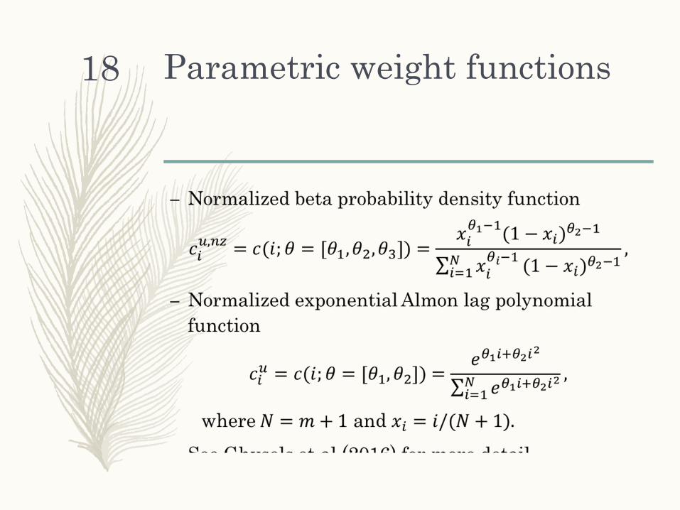
Parametric weight functions 18

Empirical studies on private equity

– The US private equity (PE) index returns from Cambridge Associates and the quarterly Fama-French benchmark factor returns from the second quarter of 1986 to the first quarter of 2016 are used.

19

US PE FF market mean 0.033 0.019 volatility 0.047 0.084 ACF(1) 0.376 -0.003

US PE returns and FF market factor

20

Identify the number of appraisal lags

21

Initial assessment

Estimate Std. Error t value Pr(>|t|) (Intercept) 0.021 0.003 7.057 0.000 L(mktQ, 0:2)0 0.376 0.039 9.582 0.000 L(mktQ, 0:2)1 0.105 0.040 2.626 0.010 L(mktQ, 0:2)2 0.125 0.040 3.158 0.002 L(smbQ, 0:2)0 0.053 0.065 0.815 0.417 L(smbQ, 0:2)1 0.063 0.066 0.950 0.344 L(smbQ, 0:2)2 -0.039 0.065 -0.603 0.547 L(hmlQ, 0:2)0 -0.077 0.043 -1.797 0.075 L(hmlQ, 0:2)1 -0.079 0.042 -1.853 0.067 L(hmlQ, 0:2)2 0.050 0.042 1.192 0.236

22

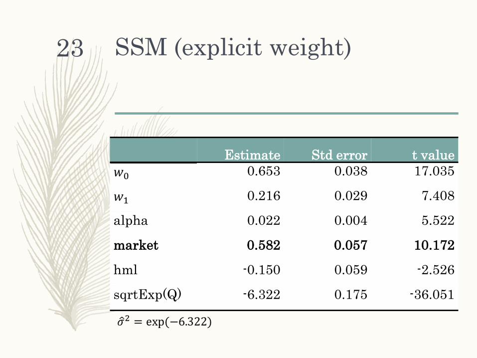
SSM (explicit weight)

Estimate Std error t value 0.653 0.038 17.035

0.216 0.029 7.408

alpha 0.022 0.004 5.522

market 0.582 0.057 10.172

hml -0.150 0.059 -2.526

sqrtExp(Q) -6.322 0.175 -36.051

23

SSM (exponential Almon lag polynomial)

Estimate Std error t value -2.094 0.740 -2.829

0.319 0.194 1.641

alpha 0.023 0.004 5.606

market 0.578 0.057 10.154

hml -0.149 0.059 -2.528

sqrtExp(Q) -6.344 0.176 -36.115

24

Comparison of appraisal weights

Ad-hoc

(market) Ad-hoc

(hml) SSM

(explicit) SSM

(parametric) 0.62 0.49 0.65 0.66

0.17 0.51 0.22 0.21

0.21 0.00 0.13 0.13

25

Appraisal frequency and the estimation of factor exposures

– Appraisal returns are usually reported on a quarterly basis (low frequency).

– Previous research assumes that assets are appraised using information at the same frequency.

– We argue that the misspecification on appraisal frequency would lead to biased estimates of the factor exposures.

– Due to time constraints, we will only show the empirical study on this topic today. Please see the working paper for more detail.

26

Econometric model for appraisal using monthly data

Mixed data sampling (MIDAS) single input distributed lag model

27

Unrestricted MIDAS regression

Estimate Std error t value ma1 0.314 0.094 3.337 ma2 0.232 0.090 2.580 intercept 0.022 0.004 5.460 X.0/m 0.479 0.065 7.421 X.1/m 0.434 0.060 7.266 X.2/m 0.325 0.053 6.100 X.3/m 0.242 0.063 3.853 X.4/m 0.135 0.061 2.210 X.5/m 0.022 0.053 0.413 X.6/m 0.127 0.064 1.975 X.7/m 0.102 0.058 1.742

28

Market beta from unrestricted MIDAS regression

– The sum of regression coefficients against contemporaneous and lagged market factors is the estimate of (long-run) market beta in a distributed lag model

X.0/m 0.479 X.1/m 0.434 X.2/m 0.325 X.3/m 0.242 X.4/m 0.135 X.5/m 0.022 X.6/m 0.127 X.7/m 0.102

29

SSM (explicit weight)

Estimate Std error t value w0 0.260 0.030 8.619 w1 0.238 0.031 7.689 w2 0.177 0.028 6.359 w3 0.117 0.025 4.666 w4 0.068 0.028 2.406 w5 0.014 0.027 0.522 w6 0.068 0.026 2.584 alpha 0.022 0.004 5.413 beta 1.847 0.189 9.772 sqrtExp(Q) -5.350 0.176 -30.397

30

SSM (normalized beta density function)

Estimate Std error t value 2.000 0.491 4.072 6.187 1.451 4.264

alpha 0.023 0.004 6.617 beta 1.427 0.132 10.792 sqrtExp(Q) -5.603 0.162 -34.688

The estimates of market beta using high frequency data are significantly larger than those estimated based on quarterly information and align with those from the cash flow approach.

31

Monthly appraisal weights of US PE (Cambridge Associates)

32

Empirical studies on private real estate

– Study the relationship between the quarterly NCREIF property index (NPI) returns and the monthly NAREIT composite index returns from 1986 Q3 to 2016 Q1.

33

NPI NAREIT* mean 0.019 0.026 volatility 0.022 0.086 ACF(1) 0.806 0.075 Remark: The squared root of time rule is used to calculate the (quarterly) statistics for NAREIT returns.

Initial assessment 34

SSM (explicit weight)

Estimate Std error t value 0.107 0.025 4.295 0.111 0.023 4.792 0.035 0.024 1.429 0.030 0.030 1.012 0.056 0.019 2.933 0.092 0.023 4.055 0.049 0.031 1.608 0.075 0.023 3.217 0.073 0.029 2.483 0.106 0.028 3.792 0.037 0.022 1.664 0.129 0.024 5.304 0.061 0.045 1.349

alpha 0.014 0.003 4.298 beta 0.606 0.103 5.864 sqrExp(Q) -5.835 0.185 -31.473

35

SSM (normalized beta density function)

Estimate Std error t value 0.426 0.092 4.637 0.735 0.114 6.452

alpha 0.015 0.003 4.475 beta 0.578 0.094 6.134 sqrtExp(Q) -5.719 0.181 -31.562

36

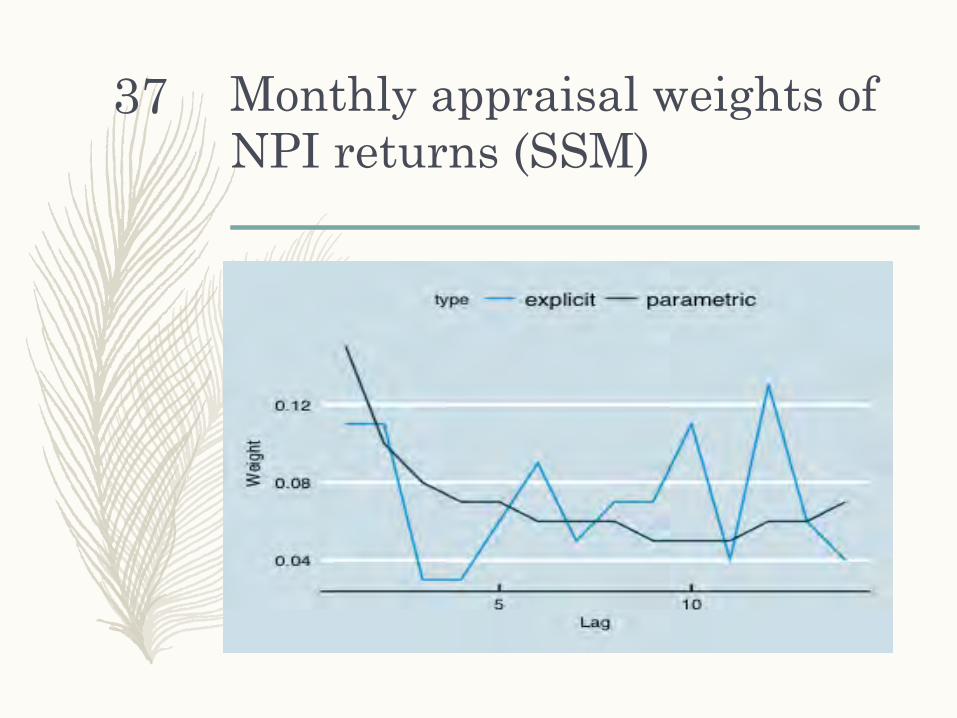
Monthly appraisal weights of NPI returns (SSM)

37

Forecast NPI returns using monthly REITs returns

38

Possible extensions Periodic appraisal scheme

39

Possible extensions Mixed frequency appraisal

– We have considered the case that assets are appraised using monthly (high frequency) data.

– In reality, assets may be appraised using mixed frequency information, such as a low frequency private factor (may be unobservable) and a high frequency public counterparty.

– This extension may be done by adding an additional state variable to Dimson’s model using high frequency information.

40

Future work

1. More work and empirical studies on two extensions

2. Statistical tests for evaluating models with different appraisal schemes

3. An R package implementing the proposed method and tests

41

Q & A

– Any suggestions and comments are welcome.

– E-mail address: – jenwen@utstat.toronto.edu, or – jenwen@gmail.com

42

Appendix

43

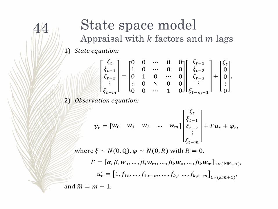
44