diplomarbeit benjamin leiber
TRANSCRIPT
Non-axially symmetric field andtrajectory calculations
for the KATRIN-experiment
Diplomarbeitvorgelegt
von
Benjamin Leiber
Am Institut für Experimentelle Kernphysik (IEKP)Karlsuhe Institute of Technology (KIT)
Referent: Prof. Dr. G. DrexlinKorreferent: Prof. Dr. W. de Boer
Bearbeitungszeit: 01. Mai 2009 – 30. April 2010
KIT – University of the State of Baden-Wuerttemberg and National Laboratory of the Helmholtz Association www.kit.edu


Erklarung
Hiermit bestatige ich, dass ich die vorliegende Arbeit selbst verfasst und keine an-deren als die angegebenen Quellen und Hilfsmittel verwendet und diese im Textkenntlich gemacht habe.
Benjamin Leiber, April 2010
iii


Zusammenfassung
Das KArlsruher TRItium Neutrino Experiment wird die Masse des Elektron An-tineutrinos mit einer Sensititvitat von 0.2 eV/c2 (90%C.L.) uber die Messung desTritium β-Spektrums in der Nahe des Endpunktes bestimmen.
Um die Energie der Zerfallselektronen zu analysieren, werden diese in einem elek-trostatischen Spektrometer nach dem MAC-E Filter-Prinzip entlang von Magnet-feldlinien gefuhrt. Durch die adiabatische Anderung des Feldes um einen Faktor von20.000 wird die transversale Energie der Zerfallselektronen in longitudinale umge-wandelt, welche dann mit dem elektrischen Retardierungspotential analysiert wird.
Zur Optimierung des experimentellen Aufbaus werden Simulationen des elektromag-netischen Designs durchgefuhrt. Dies erfordert eine flexible und modulare Software,um die auftretenden elektromagnetischen Felder und damit auch die Teilchenbahnender Zerfallselektronen im Experiment mit großer Genauigkeit zu simulieren. Beson-deres Augenmerk galt im Rahmen dieser Diplomarbeit der Nicht-Axialsymmetriedes Magnetfeldes, wie es z.B. durch Verformungen des Luftspulensystems, welchesdas Hauptspektrometer umschließt und den magnetischen Materialien in den Wan-den der Spektrometerhalle verursacht wird.
In dem nun Folgenden sollen die einzelnen Kapitel dieser Arbeit kurz vorgestellt undein kurzer Uberblick uber sie gegeben werden. Eine ausfuhrliche Darstellung inklu-sive dazugehoriger Quellenangaben ist im englischsprachigen Haupttext zu finden.
1. Einleitung Neutrinos sind seit ihrer Postulation durch W. Pauli in den 30erJahren des 20ten Jahrhundert Gegenstand intensiver Forschungen. Als “Geis-terteilchen”, die nur schwach wechselwirken entzogen sie sich lange der direktenBeobachtung und konnen auch heute nur mit Hilfe von Prozessen, in denendurch sie geladene Teilchen erzeugt werden, nachgewiesen werden.Im Standard-Modell der Teilchenphysik gelten die Neutrinos als masselos. DasSuper-Kamiokande Experiment wies jedoch durch die Beobachtung von Neutri-nooszillationen nach, dass es sich bei Neutrinos um massive Teilchen handelnmuss. Allerdings liefern Neutrino-Oszillations-Experimente keine absolutenWerte fur die Neutrinomassen, lediglich Massendifferenzen, die aus Mischver-haltnissen abgeleitet werden.Zur absoluten Massenbestimmung gibt es eine Reihe anderer Methoden, diesich grob in zwei Kategorien einteilen lassen: direkt und indirekt. Die indi-rekten Methoden leiten aus kosmologischen und astronomischen Beobachtun-gen Grenzen fur die Summe der Neutrinomassen her, die allerdings sehr starkmodellabhangig sind. Zu den direkten Nachweismethoden gehoren die Suche
v

vi
nach dem neutrinolosen Doppelbeta-Zerfall, die aber ebenfalls stark modellab-hangig ist und die kinematische Vermessung des Myon- und Tau-Zerfalls undim Speziellen die von β-Zerfallen. Diese brauchen keine Modellannahmen zutreffen, da sie nur die Impuls- und Energieerhaltung vorraussetzen. Das KA-TRIN Experiment verfolgt einen solch modellunabhangigen Ansatz und wirddas β-Spektrum des Tritium-Zerfalls nahe dessen Endpunkt vermessen.
2. Das KATRIN Experiment Die aktuelle Obergrenze fur die Masse desElektron-Antineutrinos wurde durch die beiden Experimente in Troitsk undMainz, die wie KATRIN den Tritium-β-Zerfall untersuchten, aufgestellt, undliegt bei 2.0 eV/c2. KATRIN soll diese Obergranze um eine Großenordnungverbessern und sie damit auf 0.2 eV/c2 reduzieren. Dies erfordert eine sig-nifikante Verbesserung der Hauptkomponenten des Experiments im Vergleichzu den Vorgangerexperimenten.Die Energie der Zerfallselektronen wird analog zu den Vorgangerexperimentenmit Hilfe eines sogenannten MAC-E Filters vermessen. Dieses elektrostatischeSpektrometer blockiert Elektronen unterhalb einer bestimmbaren Energie, sodass ein integriertes Spektrum aufgenommen werden kann. Ein Magnetfeld di-ent zur Fuhrung der Elektronen von der Quelle zum Detektor, gleichzeitig wirddieses innerhalb der Spektrometer so verringert, dass die transversale Energieder Elektronen in longitudinale umgewandelt wird. Dieses Prinzip heisst mag-netische adiabatische Kollimation. Im Bereich des kleinsten Magnetfeldes, dersogenannten Analysierebene erreicht das elektrische Retardierungspotentialseinen Maximalwert. Hier haben die Elektronen minimale transversale Energieund laufen gegen die Potentialbarriere an. Nur Elektronen mit großerer kinetis-cher Energie als die Barriere werden transmittiert und gelangen zum Detektor.Die Zentrale Komponente hierbei ist der MAC-E Filter, der sowohl moglichstdie gesamte transversale in longitudinale Energie umwandeln, ein hohe Trans-mittivitat fur Signal-Elektronen und eine niedrige Rate an Sekundar-Elektronenhaben soll. Es gilt also ihn in dieserlei Hinsichten zu optimieren.
3. Methoden zur elektrischen und magnetischen Feldberechnung DasZusammenspiel von statischen elektrischen und magnetischen Feldern is wichtigfur die Funktion der Spektrometer. Um ihre Eigenschaften ohne experimentellenAufwand zu studieren und um Anpassungen am elektromagnetischen Designabzuschatzen, wurden in der Vergangenheit verschiedene, auf der Program-miersprache C basierende Programme verwendet. Die Routinen zur magnetis-chen und elektrischen Feldberechnung verwenden einerseits die numerische In-tegration von elliptischen Integralen und andererseits eine Legendre-Polynom-Entwicklung, die besonders schnell ist. Im Rahmen dieser Arbeit wurden die C-Programme uberarbeitet und in eine objektoriente Form in der Programmier-sprache C++ gebracht. Sie sind nun flexibel und benutzerfreundlich in demProgrammpaket KAFCA zusammengefasst. Zusatzlich zur Modernisierungbestehender Programme wurden zwei Feldberechnungen fur nicht axialsym-metrische Magnetfelder und eine universell einsetzbare Interpolationsmethodeaus bestehenden C-routinen neu implementiert. Diese bilden das in C++geschriebene KNAXS-Programmpaket.
4. Bahnverfolgung geladener Teilchen Um die Auswirkungen der elektrischenund magnetischen Felder auf die adiabatische Enegietransformation und die
vi

vii
Transmission der Elektronen im Experiment zu untersuchen, braucht manRoutinen zur Simulation der Elektron-Bewegung. Die Bewegungsgleichungeines Elektrons im elektromagnetischen Feld ist bestimmt durch die Lorentz-Kraft. Diese lasst sich durch verschiedene Verfahren numerisch losen. DieRunge-Kutta Methoden verbinden hierbei hohe Geschwindigkeit mit ausgeze-ichneter Prazision. Zudem kann man die Bahnverfolgung durch geschickte, dy-namische Wahl der Schrittgroße weiter optimieren. Fur sehr große Schrittgroßenwird die numerische Losung der Lorentz-Gleichung allerdings sehr ungenau. Indiesem Fall besteht die Moglichkeit eine adiabatische Naherung der Teilchen-bahn zu verwenden. Bei dieser Naherung wird lediglich der Weg des Fuhrungszen-trums der Zyklotronbahn des Elektrons genau berechnet und, abhangig vomMagnetfeld, anschließend eine Bewegung senkrecht dazu addiert. Diese Naherungbietet einen enormen Geschwindigkeitsgewinn, allerdings nur in Bereichen indenen sich das Elektron adiabatisch bewegt.Dank der Flexibilitat der Runge-Kutta Methode, lassen sich damit alle moglichenDifferentialgleichungssyteme erster Ordnung losen. So kann man damit ana-log zur adiabatischen Naherung auch Feldlinien berechnen, die ebenfalls einer“Kraft” in Richtung des Feldvektors folgen.Abschließend ist es fur die Untersuchung vieler Probleme wichtig, wo sich dasTeilchen relativ zur felderzeugenden Geometrie befindet und ob es auf bes-timmte Korper wie z.B. einen Elektrodendraht oder den Detektor trifft. Zudiesem Zweck benutzt man eine dreidimensionale Abstandsberechnung, die aufeinfachen Vektorbeziehungen basiert.
5. Implementierung Die in den vorangegangenen zwei Kapiteln vorgestelltenMethoden zur Feld- und Teilchenbahnberechnung, existierten in der Mehrheitbereits als C-Programme, welche, wenn uberhaupt, nur schwer miteinander zukombinieren und zu verwenden waren. Mit Hilfe von F. Gluck, S. Mertensund mit Beitragen von N. Wandkowsky wurde wahrend dieser Diplomarbeitdie Anstrengung unternommen, die Feldberechnungsmethoden objektorientiertumzugestalten, sie zu erweitern und ein Bahnberechnungs-System zu schaf-fen, welches vielseitig und komfortabel zu bedienen ist. Erreicht wurde diesdurch languberlegte Planung und konsequente Umsetzung objektorientierterAnsatze wie das Klassen- und das Vererbungsprinzip. Dies fuhrte zu der nunexistierenden Software bestehend aus den Programmpaketen KTrack, KAFCAund KNAXS, die dank ihres logischen Aufbaus komplizierte Berechnungen miteinfacher Bedienung und hoher Geschwindigkeit verbindet.Um die Berechnunsgeschwindigkeit bei statischen Feldern weiter zu erhohenenthalt KNAXS die Hermite-3D-Interpolationsmethode, die sich durch sehrhohe Prazision bei gleichzeitig enormer Berechnungsgeschwindigkeit bei derInterpolation von homogenen Felder auszeichnet.
6. Untersuchung von Untergrund, verursacht durch nicht axialsym-metrische Felder Magnetfeldmessungen in der KATRIN-Halle und Mes-sungen der Verformung des Luftspulensystems lassen auf ein magnetischesStreufeld, das uber den ursprunglichen Erwartungen liegt schließen. Deshalbist es wichtig, die Auswirkungen solchen Streufelder auf das Experiment genauzu kennen. Mit Hilfe der KNAXS Software lassen sich Modelle, der Verformungsowie der magnetischen Materialien in Hallenwanden und -boden erstellen, diedie Messungen wiedergeben.
vii
viii
Mit diesen Modellen kann man wiederrum mit Hilfe von KTrack die Auswirkun-gen der Streufelder auf Teilchenbahnen im Experiment berechnen. Die Berech-nungen zeigen, das Signal-Elektronen nur unbedeutende Ablenkungen durchdie magnetischen Streufelder erfahren. Anders sieht es aus fur Sekundarelek-tronen, die durch Hintergrund-Strahlung und kosmische Teilchen aus den Wan-den des Hauptspektrometers ausgeschlagen werden. Es wird angenommen,dass etwa 107 solcher Teilchen pro Sekunde auf der inneren Oberflache desTanks entstehen. Die niederenergetischen von ihnen konnen gespeichert wer-den und eine radiale Drift, verursacht durch die magnetische Streufelder in denFlussschlauch vollfuhren. Da sich diese Elektronen im Maximum des Streu-querschnitts mit Restgasmolekulen befinden, ist es sehr wahrscheinlich, dasssie eine Art von Untergrundsignal durch Restgasionisierung oder Streuung inRichtung des Detektors verursachen.
7. Zusammenfassung und Ausblick Zusammenfassend lasst sich sagen, dassmit der Erweiterung und Verbesserung der vorhandenen Simulationswerkzeugeein guter Weg beschritten wurde und die Entwicklung der Programme auchin Zukunft vorangetrieben werden wird. Zudem ist es nun moglich, verhalt-nismaßig komplizierte Simulationen schnell und einfach zu konfigurieren undauch nicht-axialsymmetrische Feldbeitrage in die Bahnverfolgung mitein zubeziehen.In Zukunft wird eine große Monte-Carlo-Simulation der Elektronen, die vonden Spektrometerwanden starten, fur Vor- und Hauptspektrometer durchge-fuhrt werden, in welcher die tatsachlichen Sekundarelektronen-Verteilungenund -Spektren berucksichtigt werden. Mit Simulationen dieser Art lasst sichdie durch die magnetischen Streufelder verursachte Untergrundrate im Exper-iment studieren.
viii

Contents
1 Introduction 11.1 Evidence for massive neutrinos . . . . . . . . . . . . . . . . . . . . . . 1
1.1.1 Atmospheric neutrino anomaly . . . . . . . . . . . . . . . . . 11.1.2 The solar neutrino problem . . . . . . . . . . . . . . . . . . . 1
1.2 Neutrino oscillations . . . . . . . . . . . . . . . . . . . . . . . . . . . 31.2.1 Measurements of the parameters of neutrino oscillation . . . . 41.2.2 Conclusions . . . . . . . . . . . . . . . . . . . . . . . . . . . . 6
1.3 Direct measurements of neutrino mass . . . . . . . . . . . . . . . . . 61.3.1 β-decay . . . . . . . . . . . . . . . . . . . . . . . . . . . . . . 71.3.2 π- and τ -decay . . . . . . . . . . . . . . . . . . . . . . . . . . 91.3.3 Neutrinoless double-β-decay . . . . . . . . . . . . . . . . . . . 10
1.4 Indirect measurements of the neutrino mass . . . . . . . . . . . . . . 10
2 The KATRIN experiment 132.1 The tritium β-decay . . . . . . . . . . . . . . . . . . . . . . . . . . . 132.2 Basic setup . . . . . . . . . . . . . . . . . . . . . . . . . . . . . . . . 14
2.2.1 WGTS . . . . . . . . . . . . . . . . . . . . . . . . . . . . . . . 142.2.2 Transport section . . . . . . . . . . . . . . . . . . . . . . . . . 142.2.3 Spectrometers . . . . . . . . . . . . . . . . . . . . . . . . . . . 152.2.4 Detector . . . . . . . . . . . . . . . . . . . . . . . . . . . . . . 15
2.3 MAC-E filter . . . . . . . . . . . . . . . . . . . . . . . . . . . . . . . 162.3.1 Principle . . . . . . . . . . . . . . . . . . . . . . . . . . . . . . 162.3.2 Characteristics . . . . . . . . . . . . . . . . . . . . . . . . . . 172.3.3 KATRIN spectrometers . . . . . . . . . . . . . . . . . . . . . 202.3.4 Aircoil system . . . . . . . . . . . . . . . . . . . . . . . . . . . 222.3.5 Background . . . . . . . . . . . . . . . . . . . . . . . . . . . . 22
3 Methods for electric and magnetic field-calculation 253.1 Magnetic field calculation . . . . . . . . . . . . . . . . . . . . . . . . 25
3.1.1 Line-segment discretization methods . . . . . . . . . . . . . . 253.1.1.1 Integrated Biot-Savart . . . . . . . . . . . . . . . . . 263.1.1.2 Magnetic dipole-bars . . . . . . . . . . . . . . . . . . 27
3.1.2 Legendre polynomial expansion . . . . . . . . . . . . . . . . . 283.1.2.1 Elliptic Integrals . . . . . . . . . . . . . . . . . . . . 283.1.2.2 Zonal Harmonic Expansion . . . . . . . . . . . . . . 293.1.2.3 Application . . . . . . . . . . . . . . . . . . . . . . . 30
3.2 Electric field calculation . . . . . . . . . . . . . . . . . . . . . . . . . 323.2.1 Boundary element method . . . . . . . . . . . . . . . . . . . . 323.2.2 Legendre polynomial expansion . . . . . . . . . . . . . . . . . 34
ix

x Contents
3.3 Three-dimensional Hermite-interpolation . . . . . . . . . . . . . . . . 343.3.1 Motivation . . . . . . . . . . . . . . . . . . . . . . . . . . . . . 343.3.2 Theory . . . . . . . . . . . . . . . . . . . . . . . . . . . . . . . 35
4 Tracking of charged particles 374.1 The Runge-Kutta method . . . . . . . . . . . . . . . . . . . . . . . . 374.2 Particle motion in general force fields . . . . . . . . . . . . . . . . . . 394.3 Charged particle motion in electric and magnetic fields . . . . . . . . 394.4 Field lines . . . . . . . . . . . . . . . . . . . . . . . . . . . . . . . . . 404.5 Adiabatic approximation . . . . . . . . . . . . . . . . . . . . . . . . . 414.6 Distance calculation . . . . . . . . . . . . . . . . . . . . . . . . . . . 42
5 Code implementation 455.1 Overview . . . . . . . . . . . . . . . . . . . . . . . . . . . . . . . . . 455.2 Field classes . . . . . . . . . . . . . . . . . . . . . . . . . . . . . . . . 46
5.2.1 Magfield3 . . . . . . . . . . . . . . . . . . . . . . . . . . . . . 475.2.2 Elfield2 . . . . . . . . . . . . . . . . . . . . . . . . . . . . . . 485.2.3 Elfield32 . . . . . . . . . . . . . . . . . . . . . . . . . . . . . . 495.2.4 Elfield33 . . . . . . . . . . . . . . . . . . . . . . . . . . . . . . 495.2.5 BiotSavart . . . . . . . . . . . . . . . . . . . . . . . . . . . . . 515.2.6 MagMaterials . . . . . . . . . . . . . . . . . . . . . . . . . . . 525.2.7 Interpolation . . . . . . . . . . . . . . . . . . . . . . . . . . . 53
5.3 Tracking classes . . . . . . . . . . . . . . . . . . . . . . . . . . . . . . 545.3.1 KTrackParticle . . . . . . . . . . . . . . . . . . . . . . . . . . 555.3.2 StepSize . . . . . . . . . . . . . . . . . . . . . . . . . . . . . . 555.3.3 DiffEqSolver . . . . . . . . . . . . . . . . . . . . . . . . . . . . 565.3.4 StepComputer . . . . . . . . . . . . . . . . . . . . . . . . . . . 56
5.4 Comparison . . . . . . . . . . . . . . . . . . . . . . . . . . . . . . . . 575.4.1 Ktrack compared to singletraj.c . . . . . . . . . . . . . . . . . 575.4.2 Interpolation precision and computation time . . . . . . . . . 58
6 Investigation of background due to non-axially-symmetric fields 636.1 Magnetic shielding . . . . . . . . . . . . . . . . . . . . . . . . . . . . 636.2 Non-axially symmetric field contributions . . . . . . . . . . . . . . . . 64
6.2.1 Deformed LFCS . . . . . . . . . . . . . . . . . . . . . . . . . . 656.2.2 Magnetic materials in the building’s walls . . . . . . . . . . . 65
6.3 Particle tracks influenced by non-axisymmetric magnetic fields . . . . 66
7 Summary and outlook 69
Bibliography 71
x

1. Introduction
Since their postulation in 1930 by W. Pauli, neutrinos have been the subject of greatscientific interest. Due to their elusive nature, the observation and investigation ofneutrinos is a technically and mentally challenging branch of astroparticle physics.The observation of the oscillation of atmospheric neutrinos in 1998 by the Super-Kamiokande experiment laid the corner stone for a new generation of neutrino ex-periments. These intend to further investigate the properties of neutrinos and inparticular search for the masses of the neutrinos.This chapter will give a short overview to today’s questions in neutrino physics andthe experimental states. At first the numerous evidences for massive neutrinos willbe discussed, as they were discovered by various experiments. This is followed bya brief annotation of neutrino oscillations and their parameters. The chapter willclose with a description of the main aspects used for direct measurements of neutrinomasses, followed by an outline.
1.1 Evidence for massive neutrinos
1.1.1 Atmospheric neutrino anomaly
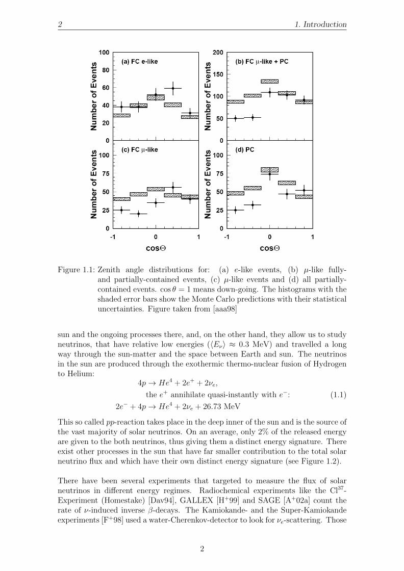
Atmospheric neutrinos are produced in interactions of cosmic rays with atomic nu-clei of the Earth-atmosphere. Experiments like Kamiokande [H+88] that used water-Cherenkov-detectors and Soudan 2 [A+97], Frejus [B+89] and NUSEX [B+82] whichused calorimeter measured the flux of atmospheric νµ and νe with directional resolu-tion. It was shown that the ratio r = νµ/νe variated with the zenith-angle (see figure1.1). The ratio rb of atmospheric neutrinos that travelled through Earth and reachedthe detector from below was found to be smaller than the ratio ra of atmosphericneutrinos that travelled a much smaller distance coming directly from above. Thiswas the first irrevocable evidence of νµ oscillating into νe and therefore non-zeroneutrino masses.
1.1.2 The solar neutrino problem
The so called solar neutrinos have their origin within the sun. Solar neutrinos areof special interest, because, on the one hand, they yield information about the inner
1
2 1. Introduction
Figure 1.1: Zenith angle distributions for: (a) e-like events, (b) µ-like fully-and partially-contained events, (c) µ-like events and (d) all partially-contained events. cos θ = 1 means down-going. The histograms with theshaded error bars show the Monte Carlo predictions with their statisticaluncertainties. Figure taken from [aaa98]
sun and the ongoing processes there, and, on the other hand, they allow us to studyneutrinos, that have relative low energies (〈Eν〉 ≈ 0.3 MeV) and travelled a longway through the sun-matter and the space between Earth and sun. The neutrinosin the sun are produced through the exothermic thermo-nuclear fusion of Hydrogento Helium:
4p→ He4 + 2e+ + 2νe,
the e+ annihilate quasi-instantly with e−:
2e− + 4p→ He4 + 2νe + 26.73 MeV
(1.1)
This so called pp-reaction takes place in the deep inner of the sun and is the source ofthe vast majority of solar neutrinos. On an average, only 2% of the released energyare given to the both neutrinos, thus giving them a distinct energy signature. Thereexist other processes in the sun that have far smaller contribution to the total solarneutrino flux and which have their own distinct energy signature (see Figure 1.2).
There have been several experiments that targeted to measure the flux of solarneutrinos in different energy regimes. Radiochemical experiments like the Cl37-Experiment (Homestake) [Dav94], GALLEX [H+99] and SAGE [A+02a] count therate of ν-induced inverse β-decays. The Kamiokande- and the Super-Kamiokandeexperiments [F+98] used a water-Cherenkov-detector to look for νe-scattering. Those
2

1.2. Neutrino oscillations 3
Figure 1.2: Solar neutrino energy spectrum for the SSM. Figure taken from [BPG04]
experiments only measured 32-64% of the solar neutrino flux predicted by the SSM1.This deficit caused the so called solar neutrino problem. An explanation for thisdisappearance of νe are the so called neutrino-flavour-oscillations. This means thatneutrinos have massive eigenstates that are not identical to the weak interactioneigenstates.
1.2 Neutrino oscillations
As the weak interaction eigenstates of the neutrinos do not correspond to their masseigenstates, they can be expressed as superposition of them:
|να〉 =∑i
Uαi|νi〉 (1.2)
with α being the neutrino flavour, i the number of the mass eigenstate and Uαi themixing matrix called Maki-Nakagawa-Sakata-Pontecorvo-matrix. The mass eigen-states |νi〉 are stationary and can be propagated into time dependent form:
|νi(t)〉 = e−iEit|νi〉 (1.3)
A flavourstate |να〉 that is pure at the time t = 0 propagates into:
|ν(t)〉 =∑i
Uαie−iEit|νi〉 =
∑i,β
UαiU∗βie−iEit|νβ〉 (1.4)
1Standard Sun Model
3
4 1. Introduction
For the transition-probability from flavour α → β, in the ultra-relativistic limit weget the transition amplitudes [GGN03], [Kay03]:
P (να → νβ) = |〈νβ(t)|να(t)〉|2 =
∣∣∣∣∣∑i
UαiU∗βie− im
2i L
2E
∣∣∣∣∣2
= δαβ − 4∑i>j
Re(U∗αiUβiUαjU∗βj) sin2
(∆m2
ijL
4E
)
+ 2∑i>j
Im(U∗αiUβiUαjU∗βj) sin2
(∆m2
ijL
2E
) (1.5)
the oscillation phase is given through ∆m2ij ≡ m2
i − m2j . This model is able to
describe the disappearance of neutrinos of a certain flavour α, depending on theirenergy and oscillation length as well as the appearance of neutrinos of a flavour βdifferent from the flavour α which was emitted at the source.
1.2.1 Measurements of the parameters of neutrino oscillation
Atmospheric neutrinos The matrix U can be decomposed into rotation matri-ces that describe the mixing between the single states νi. Data from the Super-Kamiokande experiment showed that the number of atmospheric νµ that reachedthe detector is dependent on the incident angle. The muon neutrinos that comefrom below have to travel a longer path through the Earth and therefore have agreater possibility to oscillate into tau neutrinos. With the available experimentaldata, the parameter Θ23 of the mixing matrix U was determined to a limit of:
sin2 (2Θ23) > 0.92 (1.6)
and the mass difference ∆m223 was narrowed down to the range [A+05d]:
1.5 · 10−3eV2 < ∆m223 < 3.4 · 10−3eV2 (1.7)
Solar neutrinos The SNO experiment [A+02b] was able to measure the total solarneutrino flux of all flavours, as well as the flux of electron neutrinos. To achieve this,three different reactions are used:
νe + d → p+ p+ e− Charged Current
να + d → p+ n+ να Neutral Current
να + e− → να + e− Elastic Scattering
(1.8)
The experiment came to the results that only one third of the electron neutrinosoriginating from the Sun still have their initial flavour when reaching the detector[A+05a]:
φ(νe)
φ(νe) + φ(νµ,τ )= 0.340± 0.023+0.029
−0.031 (1.9)
Knowing that the Sun only emits electron neutrinos, this measurement is a strongindicator for neutrino oscillations. Furthermore, the summed flux of all reactions isconsistent with the flux of solar neutrinos predicted by the SSM(shown in figure1.3).A global fit of all available solar neutrino data gives the oscillation parameters with
4

1.2. Neutrino oscillations 5
)-1 s-2 cm6 10× (eφ0 0.5 1 1.5 2 2.5 3 3.5
)-1
s-2
cm
6 1
0×
( τµφ
0
1
2
3
4
5
6
68% C.L.CCSNOφ
68% C.L.NCSNOφ
68% C.L.ESSNOφ
68% C.L.ESSKφ
68% C.L.SSMBS05φ
68%, 95%, 99% C.L.τµNCφ
Figure 1.3: Solar neutrino fluxes φµτ versus φe as measured by the SNO and Super-Kamiokande experiments. The dashed lines mark the neutrino flux pre-dicted by the SSM. The flux φe is given by the CC-flux (marked by apoint and lines, that represent various confidence levels) and φµτ by thedifference of the fluxes NC - CC. Figure taken from [A+05a]
1σ uncertainties:
tan2 (Θ12) = 0.45+0.09−0.08 and ∆m2
12 = 6.5+4.4−2.3 · 10−5eV2 (1.10)
Hence, the mixing angle Θ12 is quite large, but not maximal.
Reactor neutrinos Fission reactors are a copious source of electron anti-neutrinosthat are produced in the β-decays of neutron-rich nuclei. These electron anti-neutrinos are produced by the chain of β-decay of the fission products. A typicalmodern nuclear power plant has several reactor cores, each with a thermal powerof the order of 3GWth. On average, each fission produces 200MeV with release ofabout 6νe. That means the flux of electron neutrinos is about 2 · 1020s−1 per GWth.Although the anti-neutrino flux is very high, it is isotropic and decreases rapidlywith distance. Fortunately, the released anti-neutrinos have a relatively low energyin the order of a few MeV, which implies a short oscillation length.Reactor electron anti-neutrinos are detected through the inverse neutron decay pro-cess [GK07]:
νe + p→ n+ e+ (1.11)
This reaction was already used for the first detection of electron anti-neutrinos pro-duced in the Savannah River power plant. The KamLAND experiment [E+03] usedthis reaction to observe the flux of electron anti-neutrinos from nearby reactors withan average distance of about 180km. For these distances, the transition probabilitymainly depends on Θ12 and ∆m2
12 as for short distances (< 5km) the influence ofΘ12 and ∆m2
12 is negligible and the transition probability is mainly dependent onΘ13 and ∆m2
13. The experiment observed evidence for the disappearance of electron
5

6 1. Introduction
anti-neutrinos. The analysis of the measured data yields [A+05c]:
tan2 (Θ12) = 0.46 and ∆m212 = 7.9+0.6
−0.5 · 10−5eV2 (1.12)
These results can be combined with the SNO measurements of the solar neutrinosand then constrain the angle to [A+03]:
tan2 (Θ12) = 0.40+0.10−0.07 (1.13)
The Double CHOOZ collaboration is planning to set up two detectors at short dis-tances to a nuclear reactor. The experiment aims to measure sin2 (2Θ13) up to asensitivity of sin2 (2Θ13) < 0.03 at 90% C.L [Las06].
Accelerator neutrinos The neutrino beams in accelerator experiments are pro-duced through pion decay at flight, muon decay at rest and beam dump. Theseexperiments are therefore sensitive to the oscillation of a muon- into a tau-neutrino,a fact that allows the determination of Θ23 and ∆m2
23 with these kind of exper-iments. In the Japanese K2K experiment an almost pure νµ-beam was sent over250km from the KEK laboratory to the Super-Kamiokande detector. Under theassumption sin2 (2Θ12) = 1, the experimental data yields a best-fit value of the massdifference of [A+05b]:
∆m223 = 2.8 · 10−3eV2 (1.14)
Future experiments will have the primary objective to discover νµ νe oscillationsin these beams. Such a measurement would give information on the element Ue3 ofthe neutrino mixing matrix in case of three-neutrino-mixing.
1.2.2 Conclusions
The theory of neutrino oscillations is currently beeing supported by the results of awide selection of experiments. The oscillation parameters like the mixing angles orsquared mass differences have been measured or restricted. In figure 1.4 a summaryof the data presently available is shown. Still, some main issues remain unsolved:
• Absolute mass scale oscillation experiments are only sensitive to the squaredmass differences. The abolute mass scale is still to be determined.
• Mass hierarchy It is not know, how the mass eigenstates of the neutrinos areordered in respect to absolute mass. This could be hierarachical (m1 < m2 <m3) as well as inverted hierarachical (m3 < m2 < m1) or even degenerate(m3 ≈ m2 ≈ m1).
1.3 Direct measurements of neutrino mass
As we have seen in section 1.2, the results of neutrino oscillation experiments haverecently proved that neutrinos are massive. Since these experiments give only in-formation on the squared-mass-differences of the neutrino masses, it is currentlyknown that there are at least two massive neutrinos. One with a mass larger than∆m21 ≈ 9 · 10−3eV and another with a mass larger than ∆m31 ≈ 5 · 10−2eV. Anyinformation about the absolute values of the neutrino masses has to be investigatedwith other methods.
6
1.3. Direct measurements of neutrino mass 7
Cl 95%
Ga 95%
νµ↔ν
τ
νe↔ν
X
100
10–3
∆m
2 [
eV
2]
10–12
10–9
10–6
102 100 10–2 10–4
tan2θ
CHOOZ
Bugey
CHORUS NOMAD
CHORUS
KA
RM
EN
2
PaloVerde
νe↔ν
τ
NOMAD
νe↔ν
µ
CDHSW
NOMAD
K2K
KamLAND
95%
SNO
95% Super-K
95%
all solar 95%
http://hitoshi.berkeley.edu/neutrino
SuperK 90/99%
All limits are at 90%CL
unless otherwise noted
LSND 90/99%
MiniBooNE
MINOS
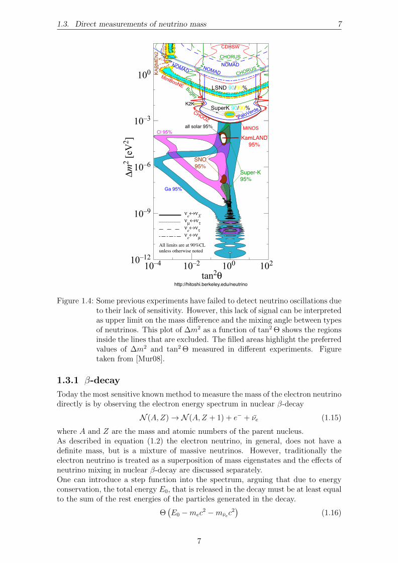
Figure 1.4: Some previous experiments have failed to detect neutrino oscillations dueto their lack of sensitivity. However, this lack of signal can be interpretedas upper limit on the mass difference and the mixing angle between typesof neutrinos. This plot of ∆m2 as a function of tan2 Θ shows the regionsinside the lines that are excluded. The filled areas highlight the preferredvalues of ∆m2 and tan2 Θ measured in different experiments. Figuretaken from [Mur08].
1.3.1 β-decay
Today the most sensitive known method to measure the mass of the electron neutrinodirectly is by observing the electron energy spectrum in nuclear β-decay
N (A,Z)→ N (A,Z + 1) + e− + νe (1.15)
where A and Z are the mass and atomic numbers of the parent nucleus.As described in equation (1.2) the electron neutrino, in general, does not have adefinite mass, but is a mixture of massive neutrinos. However, traditionally theelectron neutrino is treated as a superposition of mass eigenstates and the effects ofneutrino mixing in nuclear β-decay are discussed separately.One can introduce a step function into the spectrum, arguing that due to energyconservation, the total energy E0, that is released in the decay must be at least equalto the sum of the rest energies of the particles generated in the decay.
Θ(E0 −mec
2 −mνec2)
(1.16)
7

8 1. Introduction
We use Fermi’s Golden Rule to describe the transition probability T for the decay:
T ∝ |M|2 ρ(E) (1.17)
This means that the probability for the decay depends on the overlap between theinitial- and final-state wave functions. In case of so called “allowed” β-decays, thefinal-state wave functions of the electron and the anti-neutrino can be consideredconstant, as they are given by the nuclear matrix element |M|2. The density of theavailable final states ρ can be derived [Fer34]. We find a decay rate dependent onthe electron energy E [Wei]:
dN
dE= R(E)(E0 − E)
√(E0 − E)2 −m2
νec4Θ(E0 − E −mνec
2)
(1.18)
R(E) is a product of factors, that are not relevant for the neutrino mass determina-tion:
R(E) =G2F
2π3~7cos2 θC |M|2 F (Z + 1, E)p(E +mec
2), (1.19)
where GF is the Fermi coupling constant, θC is the Cabibbo angle,M is the nuclearmatrix element, E and p are the electron kinetic energy and momentum. F (Z+1, E)is the Fermi function that describes the electromagnetic interaction of the producedelectron with the final-state nucleus.The figure of interest in equation (1.18) is of course mνec
2, which expresses thedependency of the spectrum on the neutrino mass. If this mass is not zero, the end-point of the spectrum will shift to a lower energy whereas in regions with high countrates, the effect of the neutrino mass on the spectrum will be rather insignificant.This is plotted in figure 1.5.
coun
t rat
e [a
rb. u
nits
]
Figure 1.5: Spectra arround the β-decay endpoint E − 0 for 0 (red) and 1 eV (blue)νe-mass. Figure taken from [Hot09]
As mentioned before, we now want to take into account the effects of neutrinomixing. Therefore, we express the electron neutrino as a weighted superposition ofthe mass-eigenstates:
νe =∑i
Ueiνi (1.20)
8

1.3. Direct measurements of neutrino mass 9
Introducing this superposition into the decay spectrum gives us:
dN
dE= R(E)
∑i
|Uei|2 (E0 − E)
√(E0 − E)2 −m2
i c4Θ(E0 − E −mic
2)
(1.21)
This leads to fine structures in the spectrum, which, up to now, cannot be resolvedin measurements due to the very small mass differences (see 1.2.1). So in currentmeasurements only a weighted sum is observable:
m2νe =
3∑i=1
|Uei|2m2νi
(1.22)
Most of the parameters of the spectrum described in (1.21) are well known. Soin kinematic searches the data analysis turns out to be rather simple, as the onlyunknown quantities that have to be taken into account are the mνe and the endpointenergy E0.
1.3.2 π- and τ-decay
Another direct way to measure the neutrino mass experimentally are the pion- andtau-decays. The resulting experimental constraints are much less stringent thanthose obtained in β-decay experiments. Still these pion- and tau-decay experimentsare historically interesting as they can be used to constrain the mixing of νµ and ντwith heavy neutrinos beyond three-neutrino mixing.Measurements of the kinematics in the decay of charged pions can give informationon the neutrino masses. The most sensitive experiment up to now was performed atPSI and has used the following decay:
π+ → µ+ + νµ. (1.23)
Since this decay has a two-body final state, the mass of the neutrino can be deter-mined by energy-momentum conservation if the momenta of the pion and muon canbe measured with sufficient accuracy. In case of neutrino mixing, the muon neutrinois a superposition of different massive neutrinos. A measurement of the neutrinomass forces the superposition to collapse on the massive neutrino whose mass hasbeen measured. Therefore, in analogy to (1.21), the decay rate must have peakscorresponding to the values of the neutrino masses, which are given by
m2i = m2
π +m2µ − 2mπ
√m2µ + |~pµ|2 (i = 1, 2, 3) (1.24)
for pions decaying at rest.The value of the muon momentum measured in the PSI experiment is [A+96]:
|~pµ|2 = 29.79200± 0.00011MeV (1.25)
leading to upper limits of mi (at 90% C.L.)
mi < 0.17MeV (i = 1, 2, 3) (1.26)
The ALEPH experiment has used tau-decays for measurement of neutrino masses.The decays
τ− → 2π− + π+ + ντ and τ− → 3π− + 2π+ + ντ + π0 (1.27)
9

10 1. Introduction
have been studied, with the result (at 95%C.L.) [B+98]:
mi < 18.2MeV (i = 1, 2, 3) (1.28)
It is unlikely that in the future the measurements of neutrino masses with pion-and tau-decay experiments may improve so much to reach a precision at the eVlevel, comparable with β-decay experiments. As mentioned before, their interestlies mainly in the possibility of constraining the admixture of the muon and tauneutrinos with heavy neutrinos beyond three-neutrino mixing.
1.3.3 Neutrinoless double-β-decay
Neutrinoless double-β-decay experiments are considered as the best way to inves-tigate the Majorana nature of neutrinos. In addition, such experiments offer thepossibility of determination of the absolute neutrino mass scale and verification ofthe mass hierarchy of neutrinos.The neutrinoless double-β-decay processes of the types
N (A,Z)→ N (A,Z + 2) + 2e− (2β−0ν)
N (A,Z)→ N (A,Z − 2) + 2e+ (2β+0ν)
(1.29)
are forbidden in the SM2 if the neutrinos are Dirac particles. But they are possibleif neutrinos are massive Majorana particles. In this case, a nucleus which can decaythrough a 2β2ν process can also decay through a 2β0ν process, albeit with a differentlifetime.The Heidelberg-Moscow experiment used a well shielded Germanium-counter to lookfor the double-β decay of the isotope 76Ge into 76Se. Figure 1.6 shows the hypo-thetical spectrum of such a decay. After ten years of measurement, the data yields[KKDHK01]:
τ2ν = 1.74± 0.01+0.18−0.16 · 1021a and τ0ν = 1.5+1.68
−0.7 · 1025a (1.30)
If these results can be confirmed by other experiments with higher statistics, it wouldin fact prove that neutrinos are massive Majorana particles. The estimated neutrinomass is:
〈mν〉 = 0.39+0.45−0.34 eV (1.31)
This mass lies in a scale accessible by β-decay experiments, so that it could beconfirmed by experiments like KATRIN in the near future. Still one has to keepin mind the high model-dependence of these values: the complex Majorana phasesthat are used for the mass calculation are not known precisely, the elements of thenuclear transition matrix are not known with sufficient precision and there couldbe other theoretical explanations for the neutrinoless double β-decay than massiveneutrinos, as for example super-symmetric particles or right-handed weak-couplings.
1.4 Indirect measurements of the neutrino mass
Cosmology offers several ways to indirectly determine the neutrino mass from vari-ous experimental data. However, most of them are only sensitive to the sum of the
2Standard Model
10

1.4. Indirect measurements of the neutrino mass 11
Figure 1.6: Energy spectrum of a double-β-decay. The continuum stands for thesummed energy of both charged leptons from the 2β2ν-decay. The mo-noenergetic line at the total energy of the transition derives from the2β0ν-decay. Figure taken from [BSS]
masses of all neutrinos and the results are very model-specific [Han05].
When a supernovae transforms into a neutron star through the fusion of electronsand protons there are many neutrinos created. The time of flight of one neutrino toa detector on the Earth depends on its energy and mass. From the time differencebetween the detection of neutrinos from the same supernova and their measured en-ergy an upper limit between 5.7 eV and 23 eV for the mass of the ν3 can be derived.These values are very dependent on model-assumptions and the analysis-method[LL02], [KST87].
From the analysis of the structure of the cosmic microwave background radiationand a comparison with the estimated distribution of matter in the universe, an upperlimit for the sum of all neutrino masses between 0.42 eV and 1.8 eV can be derived[Han05].
11


2. The KATRIN experiment
The goal of the KATRIN experiment [O+] is to determine the mass of the electronanti-neutrino by examining the shape of the tritium-β-spectrum close to its end-point. With approximately 1000 days of data-taking, the experiment will be able toachieve a mass determination down to 0.35 eV/c2 (5σ) or to set an upper limit of0.2 eV/c2 (3σ) [Col04].The following chapter will give a short introduction to the experiment, briefly de-scribing the basic mechanics and its core components.
2.1 The tritium β-decayAs KATRIN is built to perform an ultra-precise measurement of the kinematics ofβ-decay electrons, the β-source is of very special importance. For the KATRINexperiment, it was decided to use the hydrogen-isotope tritium (3H) because it hasthe following key advantages.
• low endpoint energy The β-spectrum of tritium has an endpoint-energy of18.57 keV thus being the β-emitter with the second lowest energy of all possiblecandidates.
• short half-life Tritium is a rather short-lived isotope, having a half-life ofonly 12.3 a. This has the advantage that there is less source material neededin order to reach an adequate count rate and shortens the measurement time.
• simple electron shell The electron shell configurations of tritium and itsdaughter 3He
+are quite simple. This is also true for their molecular states.
The atomic and molecular corrections and the corrections due to the interac-tion with the emitted electron can be precisely computed [DT08], [ReW83].
• small inelastic scattering probability As tritium has a low nuclear chargeZ the probability for inelastic scattering of emitted β-decay electrons withinthe source will be small.
• nuclear matrix element The tritium β-decay is super-allowed as it is atransition between mirror nuclei. Thus the nuclear matrix elements are energyindependent and no corrections from the nuclear transition matrix elementsM have to be taken into account.
13

14 2. The KATRIN experiment
An alternative to tritium would be 187Rh, which has the lowest endpoint energy (2.47keV) of all known β-decay nuclei. The MARE experiment [Hal06] will use arraysof low temperature calorimeters to measure the Rhenium-187-β-spectrum. It aimsfor a sensitivity comparable to the current m2
νe-limits set by the Mainz and Troitskexperiments. As this calorimetric approach offers scalability, they plan to reach asub-eV sensitivity in the future.
2.2 Basic setup
(a) (b) (c)(d)
(e)(f)
Figure 2.1: Overview of the KATRIN experimental setup, showing: the WGTS(a),the transport section(b), the pre-spectrometer(c), the main spectrome-ter(d), the detector(e) and the rear section(f).
2.2.1 WGTS
WGTS stands for windowless gaseous tritium source, which will be the source ofβ-electrons, analysed in the experiment. The ultra-cold (27 K) molecular tritium gaswith high isotopic purity (>95%) will be injected into the middle of the 10 m longsource tube and diffuses towards both ends. The inner tube has a diameter of 0.09 mand has two turbo-molecular pumps sitting at its ends to reduce the gas flow out ofthe WGTS. By controlling the temperature and the injection rate, the column den-sity within the tube will be fixed to the reference value ρ d = 5 · 1017 molecules/cm2,which grants optimal conditions with regard to both luminosity and scattering of β-electrons on residual gas molecules. In addition, the whole source tube is surroundedby superconducting solenoids that deploy a magnetic field strong enough (3.6 T) toguide the β-electrons out of the source towards the transport section.
2.2.2 Transport section
As the β-electrons from the source need to reach the spectrometers, the tritium gasfrom the source cannot be contained with physical barriers, hence why it is called“windowsless”. However, with respect to background reduction it is crucial that thetritium gas in the source must not get into the detector. Therefore, the gas flow fromthe source must be reduced by 14 orders of magnitude. For this purpose, there aretwo different pumping sections deployed between the source and the spectrometers.The Differential Pumping Section which houses turbo-molecular pumps to reducethe gas flow and the Cryogenic Pumping Section, in which the inner beam-tube iscovered by argon-frost, to which residual gas molecules are frozen up. In addition,the beam-tube follows a zig-zag-pattern, that increases the efficiency of the residualgas removal. Similar to the WGTS, the electrons in the transport section are guidedalong a high magnetic field (up to 5.6 T) generated by superconducting solenoids.
14

2.2. Basic setup 15
2.2.3 Spectrometers
The β-electrons coming from the source will be analysed by a set of electrostaticretarding spectrometers of the MAC-E-Filter type. Only those electrons with largeenough energy will pass this filter, while all others will be rejected. This will beaddressed in detail in section 2.3
2.2.4 Detector
As the energy analysis is done by the spectrometers, the detector just needs to countthe β-electrons that pass the main spectrometer. Nevertheless the detector still needsto have a good energy resolution in order to be able to discriminate between signal-and background-electrons. The detector has to meet some high requirements:
• low intrinsic background
• ability to operate in high magnetic fields
• sensitive to low count rates
• ability to cope with high rates during calibration phases
• spatial resolution, take into account the potential depression in the analysingplane
A silicon drift detector will be used with an aimed resolution of 600 eV for electronenergies about 18.6 keV. Due to the low count rates that are expected at the veryhigh energetic end of the spectrum, the detector must be well shielded to suppressexternal background. To achieve spatial resolution, the detector is segmented into148 pixels, each of them covering a part of the flux tube with the same size (seefigure 2.2).
Figure 2.2: Sketch of the detector showing all 148 separated pixels.
15

16 2. The KATRIN experiment
2.3 MAC-E filter
Most of the information concerning the neutrino mass is contained in the regionjust below the energy endpoint E0. But only a fraction 10−12 to 10−13 of all decaysreside in the area of 1 eV below E0. In order to achieve a significant count rate nearthe endpoint a spectrometer with a large angular acceptance and a good energyresolution at E0 is needed. The KATRIN spectrometers fulfil these requirementsby implementing the principle of magnetic adiabatic collimation, and analysing theelectron-energy with an electrostatic filter, or short: the MAC-E filter.
A
B
D
D
B
C
E
Figure 2.3: Sketch of the KATRIN-pre-spectrometer as an example for a MAC-Efilter. It shows the spectrometer hull/massive electrodes (A), which areput on negative potential, the superconducting solenoids (B) and theinner wire-electrodes (D). In addition, magnetic field lines(C) and anexemplary electron-trajectory (E) are displayed.
0
Figure 2.4: This figure shows an exaggerated cyclotron motion of an electron flyingthrough the spectrometer. The arrows below indicate the momentum ofthe electron with respect to the magnetic field, neglecting the change ofthe momentum due to the electric field.
2.3.1 Principle
The MAC-E filter principle is based on the idea of adiabatic guidance of electronson a cyclotron motion around magnetic field lines. As the strength of the magneticfield slowly decreases, the momentum of the electrons perpendicular to the magneticfield lines p⊥ is being transformed into the momentum parallel to the magnetic field
16

2.3. MAC-E filter 17
lines p‖. At the position of minimal magnetic field strength Bmin the electrostaticretarding potential reaches its maximum absolute value U0. Merely electrons witha certain minimum parallel momentum p‖ and therefore, minimum parallel kineticenergy
E‖ > qU0 (2.1)
are able to pass this potential barrier. Hence the MAC-E filter acts as a so calledhigh-pass filter and the measurements will deliver an integrated spectrum. Further-more, the adiabatic guidance of electrons along the magnetic field-lines means thatthe electrons always move in the same flux-tube, with a constant magnetic flux. Thisflux-tube becomes larger as the magnetic field becomes weaker, therefore a MAC-E filter needs to have the largest radius in the area of the minimal magnetic fieldstrength.
2.3.2 Characteristics
AdiabacityIn the non-relativistic approximation, E⊥ and E‖ can be expressed as follows:
Ekin =p2
2m= E‖ + E⊥,
E‖ = Ekin · cos2 Θ,
E⊥ = Ekin · sin2 Θ.
(2.2)
If the magnetic flux enclosed by the gyrating trajectory of the electron is constant,the motion is called adiabatic. Adiabatic electron motion is achieved, if the magneticfield along the cyclotron motion changes only slightly. As the magnetic field andelectric potential vary, the cyclotron radius is resized, thus containing a constant flux.With the prequisite of conserved enclosed magnetic flux the adiabatic invariant isdefined as:
Φ =
∫~Bd ~A = const =⇒ Br2
c = const. (2.3)
Another formulation for adiabatic motion is the conservation of the product of theabsolute value of the orbital magnetic moment |~µ| and the Lorentz-factor γ = 1√
1− v2c2
γµ = const. (2.4)
In the tritium decay, the maximum occurring Lorentz-factor is 1.04, thus equation(2.4) can be approximated by only considering the magnetic moment:
µ =E⊥B
= const. (2.5)
Energy resolutionAs denoted in 2.3.1, the momentum and the kinetic energy of electrons performinga cyclotron motion along the magnetic fieldlines accordingly can be divided into alongitudinal component, parallel to the magnetic field lines (p‖, E‖) and a transversalcomponent, perpendicular to the magnetic field lines (p⊥, E⊥). These componentsare defined by the polar angle Θ between the momentum of the electron ~p and themagnetic field at its position ~B see figure 2.5. So this is the main condition, that
17

18 2. The KATRIN experiment
~p‖
~p⊥
~B
~p
Θ
Figure 2.5: Definition of the angle Θ.
a MAC-E filter has to fulfil. One can also derive from this an expression for the socalled energy resolution ∆E of a MAC-E filter. It is assumed that the motion isadiabatic and the electron has its maximum kinetic energy Ekin,max stored in the per-pendicular component at the point with maximum magnetic field Bmax (Θ = 90).Then the remaining energy ∆E⊥ that is still stored in the perpendicular momentumat the point of minimum magnetic field Bmin can be determined by the relation
Ekin,maxBmax
=∆E⊥Bmin
. (2.6)
Meaning that ∆E⊥ cannot help to pass the potential barrier. For the KATRINmain spectrometer the maximum magnetic field strength is Bmax = 6 T at the pinchmagnet. The minimum value Bmin = 3 · 10−4 T is present in the middle of thespectrometer, the so called analysing plane. With the tritium endpoint energy atapproximately E0 = 18600 eV we get an energy resolution of:
∆E⊥ =Bmin
Bmax
E0 =3 · 10−4 T
6 T· 18600 eV = 0.93eV. (2.7)
The transversal energy is transformed into longitudinal energy, and simultaneously,the electric potential reduces the longitudinal energy. Therefore, the possible polarangle Θ an electron has at the analysing plane ranges fromt 0 to 90.
Transmission functionOne of the most important attributes of a MAC-E filter is its transmission function.It can be described as relative detected rate over kinetic surplus energy of the signal-electrons. Ideally this would be a step function, but as the spectrometer has a finiteresolution it typically looks like the example shown in figure 2.6. To determine thetransmission function of a MAC-E filter we have to investigate which initial condi-tions at the entrance of the spectrometer an electron has to fulfil in order to pass thefilter. This is mainly defined by the relation between the initial transversal energyE⊥,start of the electron (which can be expressed in terms of the initial angle Θstart
with respect to the magnetic field) and the retarding potential U0 at the positionwhere the electron will pass the filter. Following equation (2.1) only electrons that
18

2.3. MAC-E filter 19
0
0.2
0.4
0.6
0.8
1
-0.4 -0.2 0 0.2 0.4 0.6 0.8 1 1.2 1.4
norm
aliz
ed r
ate
E-qU [eV]
Figure 2.6: Theoretical transmission function of a MAC-E filter.
have enough longitudinal energy can pass the spectrometer:
E‖,Bmin > 0 =⇒ E‖,Bmin = Ekin,Bmin − E⊥,Bmin= Ekin,Bmin − E⊥,Bstart
Bmin
Bstart
= Ekin,Bstart − qU0 − Ekin,Bstart sin2 ΘstartBmin
Bstart
=⇒ qU0 > Ekin,Bstart
(1− sin2 Θstart
Bmin
Bstart
).
(2.8)
Where the indices min and start describe the conditions in the analysing plane andat the entrance of the filter respectively. Furthermore we can limit the maximumaccepted Θ of transmitted electrons to:
=⇒ Θstart ≤ arcsin
√Ekin − qU0
Ekin
Bstart
Bmin
. (2.9)
So only electrons with an angle smaller than Θstart at the entrance of the filter areable to pass the potential barrier. With the fraction of electrons passing the fil-ter compared to the overall electrons being sent through the filter the transmissionfunction can be determined. From equation (2.9) we get the solid angle ∆Ω. Com-paring ∆Ω with the maximal solid angle 2π (forward direction) gives the fraction ofelectrons that are accepted by the filter:
∆Ω
2π= 1− cos Θ. (2.10)
Combining these two equations we get the transmission function T (Ekin, U0) of theMAC-E filter:
T (Ekin, U0) =
0 for Ekin < qU0
1−√
1− Ekin−qU0
Ekin
BstartBmin
for qU0 ≤ Ekin ≤ qU0
1− BminBstart
1 for qU0
1− BminBstart
≤ Ekin
(2.11)
19
20 2. The KATRIN experiment
In order to measure this transmission function, monoenergetic electron sources areemployed. Because the kinetic energy of the electrons Ekin is constant, either theretarding potential U0 has to be varied or an additional, variable acceleration poten-tial has to be applied to the source. One can also see from equation (2.11) that, inthe case of a perfectly monoenergetic source, the width of the transmission functionsolely depends on the ratio Bmin
Bstartof the magnetic fields. The width increases if a
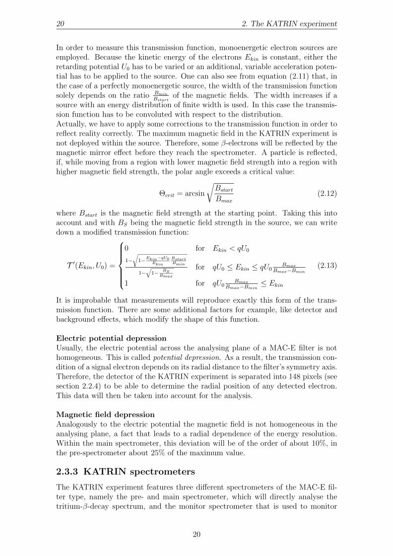
source with an energy distribution of finite width is used. In this case the transmis-sion function has to be convoluted with respect to the distribution.Actually, we have to apply some corrections to the transmission function in order toreflect reality correctly. The maximum magnetic field in the KATRIN experiment isnot deployed within the source. Therefore, some β-electrons will be reflected by themagnetic mirror effect before they reach the spectrometer. A particle is reflected,if, while moving from a region with lower magnetic field strength into a region withhigher magnetic field strength, the polar angle exceeds a critical value:
Θcrit = arcsin
√Bstart
Bmax
(2.12)
where Bstart is the magnetic field strength at the starting point. Taking this intoaccount and with BS being the magnetic field strength in the source, we can writedown a modified transmission function:
T ′(Ekin, U0) =
0 for Ekin < qU0
1−√
1−Ekin−qU0Ekin
BstartBmin
1−√
1− BSBmax
for qU0 ≤ Ekin ≤ qU0Bmax
Bmax−Bmin
1 for qU0Bmax
Bmax−Bmin ≤ Ekin
(2.13)
It is improbable that measurements will reproduce exactly this form of the trans-mission function. There are some additional factors for example, like detector andbackground effects, which modify the shape of this function.
Electric potential depressionUsually, the electric potential across the analysing plane of a MAC-E filter is nothomogeneous. This is called potential depression. As a result, the transmission con-dition of a signal electron depends on its radial distance to the filter’s symmetry axis.Therefore, the detector of the KATRIN experiment is separated into 148 pixels (seesection 2.2.4) to be able to determine the radial position of any detected electron.This data will then be taken into account for the analysis.
Magnetic field depressionAnalogously to the electric potential the magnetic field is not homogeneous in theanalysing plane, a fact that leads to a radial dependence of the energy resolution.Within the main spectrometer, this deviation will be of the order of about 10%, inthe pre-spectrometer about 25% of the maximum value.
2.3.3 KATRIN spectrometers
The KATRIN experiment features three different spectrometers of the MAC-E fil-ter type, namely the pre- and main spectrometer, which will directly analyse thetritium-β-decay spectrum, and the monitor spectrometer that is used to monitor
20

2.3. MAC-E filter 21
-18583.6
-18583.4
-18583.2
-18583
-18582.8
-18582.6
-18582.4
-18582.2
-18582
0 0.5 1 1.5 2 2.5 3 3.5 4 4.5
reta
rdin
g po
tent
ial [
U]
radius [m]
0.00031
0.000315
0.00032
0.000325
0.00033
0.000335
0.00034
0.000345
0.00035
0.000355
0 0.5 1 1.5 2 2.5 3 3.5 4 4.5
mag
netic
fiel
d [T
]
radius [m]
Figure 2.7: radial depression of the electric potential (left) and magnetic field (right)in the analysing plane of the KATRIN mainspectrometer
the stability of the main spectrometer retarding potential.
Monitor spectrometerIn order to achieve the desired sensitivity for the neutrino mass of the KATRINexperiment, the retarding potential of the analysing spectrometer has to be knownwith a precision of 4 ppm at 18.6 kV. In order to control this, a real-time calibrationexperiment will be run in parallel, occupying the so called monitor spectrometer.This apparatus was already utilised in the Mainz Neutrino Mass Experiment toanalyse the β-decay spectrum of a condensed tritium film and has been transferredto the KATRIN experimental site in late 2009. During operation, the spectrome-ter will be connected to the retarding potential of the main experiment, analysingnuclear electron sources and by this monitoring the potential with the help of wellknown nuclear standards.
Pre-spectrometerThe pre-spectrometer if of importance for the KATRIN experiment during both, theconceptional phase and the actual measurements. It serves as a prototype for themain-spectrometer by investigating the vacuum concept including the heating- andcooling-system and by optimizing the electromagnetic design especially with respectto background. Later, during the tritium measurements the pre-spectrometer willserve as additional MAC-E filter, prior to the main spectrometer to reflect all elec-trons with energies E . E0 − 300 eV. This results in a reduction-factor of 106 forβ-decay-electrons that reach the main spectrometer. The pre-spectrometer is 3.4 mlong, has a diameter of 1.7 m and will be operated with a pressure of about 10−11
mbar. It achieves an energy resolution of ∆E ≈ 100 eV. It arrived at KIT in late2003 and has been used for tests since then.
Main spectrometerThe main MAC-E filter and thereby measuring tool of the KATRIN experiment isthe main spectrometer. It is about 23 m long and has a inner radius of 4.5 m witha operating pressure below 10−11 mbar. Similar to the pre-spectrometer, its vesselhull can be put on high voltage and it features an inner electrode system of wireelectrodes for potential shaping and background reduction. Two superconductingsolenoids are positioned at the ends of the spectrometer to provide the magneticguiding field. Furthermore, the spectrometer is surrounded by a system of cable
21

22 2. The KATRIN experiment
loops, the so called the aircoil system which is responsible for fine-tuning the mag-netic field shape and strength and compensation of magnetic stray fields. With amaximum magnetic field of 6 T within the superconducting coils and a minimummagnetic field of about 3 G in the analysing plane it features an energy resolutionof ∆E = 0.93 eV.
2.3.4 Aircoil system
In regions of low magnetic field like in the analysing plane of the mainspectrometer,the Earth’s magnetic field is not negligible and has a strong influence on the magneticfield inside the spectrometer. A hereby caused deformation of the flux-tube wouldlead to the loss of signal electrons and, at the same time, imply a rigorous increaseof background electrons that are guided from the wall towards the detector (seefigure 2.8). To avoid such a distortion, the KATRIN mainspectrometer featuresa so called aircoil system consisting of the Earth’s Magnetic field CompensationSystem (EMCS) and the Low Field Correction System (LFCS). The EMCS willcompensate the vertical and horizontal, non-axisymmetric component of the Earth’smagnetic field. It consists of 16 vertical and 10 horizontal cosine coils. To have thefluxtube fit into the mainspectrometer at the analysing plane the LFCS will apply amagnetic field additionally to the superconducting solenoids sitting at the connectionports(see figure 2.8). The LFCS consists of 15 large coils, whose rotational symmetryaxis is the beamtube. Having them run with individually up to 1500 Ampere-turns,they assure the desired flux-tube form that fits into the spectrometer. For moreinformation see [GMO+09].
fluxtube 191Tcm²
fluxtube 191Tcm²
Figure 2.8: Sketch of the mainspectrometer without any magnetic filed compensa-tion (left) and with the EMCS compensating the Earth’s magnetic field(right).
2.3.5 Background
Predecessor experiments have shown that there are several non negligible mecha-nisms that can lead to the creation of background-electrons within a MAC-E filter:
• ionisation of residual gas, through either signal electrons or
• particles stored in penning traps and the magnetic bottle of the filter,and
• electrons emitted from the vessel hull.
22

2.3. MAC-E filter 23
fluxtube 191Tcm²
aircoils
Figure 2.9: Sketch of the mainspectrometer with both, EMCS and LFCS installed.It is clearly visible that the flux-tube then fits into the spectrometer.
The ionisation of residual gas will be suppressed due to the very low operating pres-sure of 10−11 mbar or less inside the spectrometer vessels. This has already beentested by predecessor experiments and test measurements at the pre-spectrometer.Penning traps are created in areas with an axial magnetic field and a minimum in theelectrostatic potential. If there is a flaw in the electrode designed, there are severalpenning traps existent within a MAC-E filter. The particles stored within the trapscan cause enormous background through ionisation of residual gas by electrons andphotons, coming from photo-emission out of the traps. To prevent this, one must bevery careful when designing the electrodes and must pay special attention to avoidformation of penning traps.High energetic particles that get into the filter can be stored through the magneticmirror effect. In order to remove them from the spectrometers, there is the possibil-ity to apply an electric dipole field that guides those particles to the vessel walls orout of it.
magnetic field
U0
U < U0
Figure 2.10: Sketch showing the principle of a penning trap: The magnetic fieldconstrains the particle vertically, whereas the potential minimum con-strains it horizontally
Electrons emitted from the vessel hull could be induced by cosmic rays, environmen-tal radiation, intrinsic radioactivity or field-emission due to flawed electrode design.The last mentioned cause is easily avoided but it is impossible to shield the mainspec-trometer from outside radiation. Therefore a mechanism is needed, that preventsbackground electrons , emitted from the vessel hull, from getting into the flux tube
23
24 2. The KATRIN experiment
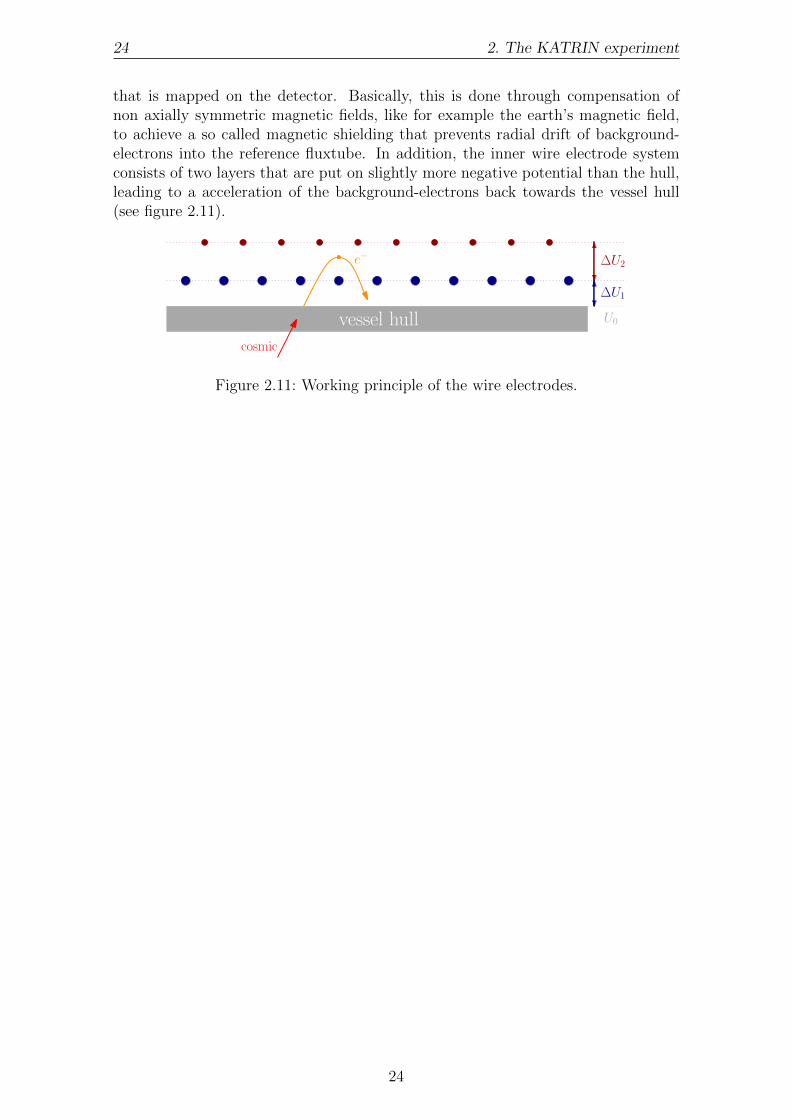
that is mapped on the detector. Basically, this is done through compensation ofnon axially symmetric magnetic fields, like for example the earth’s magnetic field,to achieve a so called magnetic shielding that prevents radial drift of background-electrons into the reference fluxtube. In addition, the inner wire electrode systemconsists of two layers that are put on slightly more negative potential than the hull,leading to a acceleration of the background-electrons back towards the vessel hull(see figure 2.11).
vessel hull
∆U1
∆U2
U0
e−
cosmic
Figure 2.11: Working principle of the wire electrodes.
24

3. Methods for electric andmagnetic field-calculation
The ability to calculate electric and magnetic fields, generated by all kinds of geome-tries and bodies is very important for an experiment whose main components arebased on an exact interplay of the very same. Field-simulation-tools are importantfor electro-magnetic design calculations as well as for investigations of a wide spec-trum of difficulties in connection with the trajectories of charged particles, as forexample, investigations of penning traps or simulations of transmission functions.Most of the methods presented in this chapter where originally developed and im-plemented in C-code by Dr. Ferenc Gluck [Glu06] at the KIT. The existing codehas been rewritten, restructured and improved in the context of this diploma thesisand was brought into an object oriented shape using C++. An implementation ofthe line-segment and interpolation methods did not exist before, they were newlywritten.
3.1 Magnetic field calculation
The magnetic fields in the KATRIN experiment are of special interest, as they doboth, guide the electrons through the experiment and grant an adiabatic transforma-tion of the electron-momentum in the spectrometers. Depending on the generatingcomponent, there are several ways to calculate the resulting magnetic field: theline-segment methods are able to emulate complex forms by composing them of nu-merous small lines, thus being flexible but slow. In contrast to them, the Legendrepolynomial methods are very fast, but need pre-calculations and are only applica-ble to axisymmetric coils. This section will give an introduction to these methods,explaining the physical and mathematical principles they are based on.
3.1.1 Line-segment discretization methods
Usually, when simulating an existing, real experimental configuration, one reachesthe point where the field-generating components can no longer be seen as simplegeometric shapes. Nevertheless, the common way to simulate them is to approximate
25

26 3. Methods for electric and magnetic field-calculation
their real geometric shape with line-segments. This method is very popular, becauseit offers the opportunity to scale the discretization of the emulated object. The usercan choose either an inaccurate model that is fast to compute, or a very accuratemodel, thus taking a lot of computation time.
3.1.1.1 Integrated Biot-Savart
In the KATRIN experiment, there are a few components, generating magnetic fieldsthat have a relatively simple shape, consisting of just a conductor that is shapedor wound in a distinct way. There are for example the components of the air coilsystem(see also 2.3.4): the EMCS, that consists of several cosine coils and the LFCSthat features some non-circular coils. Further applications will also include calcu-lating the magnetic field of the dipole coils in the DPS1-R, DPS1-F and the rearsection. To compute their effects on the magnetic field in the experiment the inte-grated Biot-Savart method is used.The magnetic field that is generated by any current-carrying component can be de-scribed using Biot-Savart’s law: From an infinitely long conductor segment withcurrent I, an infinitesimally small segment d~l in direction of the current generatesat the position ~r the magnetic field:
d ~B =µ0
4π
Id~l × rr2
. (3.1)
~I~B
P
A1
A2
~r1
~r2
Figure 3.1: A line-current-segment is defined by a start point A1, an endpoint A2
and the magnitude of the current ~I that flows from A1 to A2.
As we want to discretize our objects down to finite line-current segments, similar tothe one shown in figure 3.1, we integrate along a line current segment and get:
~Bi =µ0
4πd~L× ~I with
d~L =
(r1 + r2
R + l− r1 + r2
R− l
),
R = |~r1|+ |~r2|, l = |~r2 − ~r1| and ri =~ri|~ri|
.
(3.2)
26
3.1. Magnetic field calculation 27
Being able to use the superposition principle, it is possible to approximate complexshapes by numerous line-current-segments and simply sum up their individual fieldcontributions ~Bi to get the overall resulting magnetic field:
~Btotal =N∑i=1
~Bi (3.3)
Geometries composed of such line current segments can easily be tested by checkingthe validity of the Maxwell-equations. If, for example, the curl of the magnetic field~∇× ~Btotal is non-zero in vacuum, this is a hint that a current loop is not closed andthat you should check your discretization.
3.1.1.2 Magnetic dipole-bars
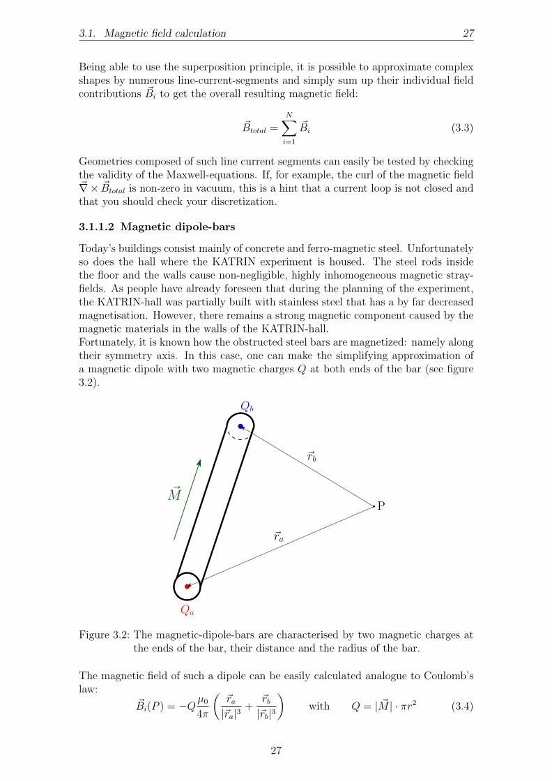
Today’s buildings consist mainly of concrete and ferro-magnetic steel. Unfortunatelyso does the hall where the KATRIN experiment is housed. The steel rods insidethe floor and the walls cause non-negligible, highly inhomogeneous magnetic stray-fields. As people have already foreseen that during the planning of the experiment,the KATRIN-hall was partially built with stainless steel that has a by far decreasedmagnetisation. However, there remains a strong magnetic component caused by themagnetic materials in the walls of the KATRIN-hall.Fortunately, it is known how the obstructed steel bars are magnetized: namely alongtheir symmetry axis. In this case, one can make the simplifying approximation ofa magnetic dipole with two magnetic charges Q at both ends of the bar (see figure3.2).
Qa
Qb
P
~rb
~ra
~M
Figure 3.2: The magnetic-dipole-bars are characterised by two magnetic charges atthe ends of the bar, their distance and the radius of the bar.
The magnetic field of such a dipole can be easily calculated analogue to Coulomb’slaw:
~Bi(P ) = −Qµ0
4π
(~ra|~ra|3
+~rb|~rb|3
)with Q = | ~M | · πr2 (3.4)
27

28 3. Methods for electric and magnetic field-calculation
~M denotes the magnetisation and r the radius of the dipole-bar. Again, to get thetotal magnetic field from all dipole-bars their contributions Bi have to be summedup. However, as the steel in the buildings is enclosed by concrete and thereby notaccessible for direct measurements of the magnetization, it is quite complicated tobuild a model to describe them them [Rei10]. In order to get an appropriate model,many magnetic field measurements near the walls of the KATRIN hall are necessary.With this data and an assumed distribution of the steel bars in the wall, one canpost a set of linear equations. The solution of these linear equations leads to a goodmodel for the magnetisation which enables us to calculate the magnetic field due tomagnetic materials in the KATRIN hall.
3.1.2 Legendre polynomial expansion
3.1.2.1 Elliptic Integrals
The main components generating magnetic fields in the KATRIN experiment arecircular coils and superconducting solenoids. These are simple circular current loops,that have a rotational symmetry axis (compare fig. 3.3).
a
z − axis
r
z
~I
Bz
Br
Figure 3.3: A loop with the radius a and the current ~I running through it, inducesa magnetic field ~B
The Biot-Savart law (3.1) for a thin coil can be expressed in terms of the completeelliptic integrals:
K(k) =
π2∫
0
dϕ√1− k2 sin2 ϕ
(I)
E(k) =
π2∫
0
dϕ
√1− k2 sin2 ϕ (II)
Π(c, k) =
π2∫
0
dϕ
(1− c2 sin2 ϕ)√
1− k2 sin2 ϕ(III)
(3.5)
28
3.1. Magnetic field calculation 29
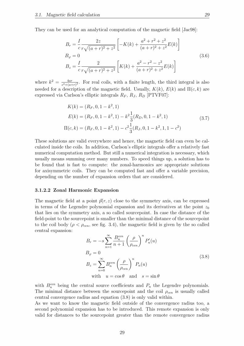
They can be used for an analytical computation of the magnetic field [Jac98]:
Br =I
c
2z
r√
(a+ r)2 + z2
[−K(k) +
a2 + r2 + z2
(a+ r)2 + z2E(k)
]Bϕ = 0
Bz =I
c
2
r√
(a+ r)2 + z2
[K(k) +
a2 − r2 − z2
(a+ r)2 + z2E(k)
] (3.6)
where k2 = 4arz2+(a+r)2
. For real coils, with a finite length, the third integral is also
needed for a description of the magnetic field. Usually, K(k), E(k) and Π(c, k) areexpressed via Carlson’s elliptic integrals RF , RJ , RD [PTVF07]:
K(k) = (RF , 0, 1− k2, 1)
E(k) = (RF , 0, 1− k2, 1)− k2 1
3(RD, 0, 1− k2, 1)
Π(c, k) = (RF , 0, 1− k2, 1)− c2 1
3(RJ , 0, 1− k2, 1, 1− c2)
(3.7)
These solutions are valid everywhere and hence, the magnetic field can even be cal-culated inside the coils. In addition, Carlson’s elliptic integrals offer a relatively fastnumerical computation method. But still a numerical integration is necessary, whichusually means summing over many numbers. To speed things up, a solution has tobe found that is fast to compute: the zonal-harmonics are appropriate solutionsfor axisymmetric coils. They can be computed fast and offer a variable precision,depending on the number of expansion orders that are considered.
3.1.2.2 Zonal Harmonic Expansion
The magnetic field at a point ~p(r, z) close to the symmetry axis, can be expressedin terms of the Legendre polynomial expansion and its derivatives at the point z0
that lies on the symmetry axis, a so called sourcepoint. In case the distance of thefield-point to the sourcepoint is smaller than the minimal distance of the sourcepointto the coil body (ρ < ρcen, see fig. 3.4), the magnetic field is given by the so calledcentral expansion:
Br = −s∞∑n=1
Bcenn
n+ 1
(ρ
ρcen
)nP ′n(u)
Bϕ = 0
Bz =∞∑n=0
Bcenn
(ρ
ρcen
)nPn(u)
with u = cos θ and s = sin θ
(3.8)
with Bcenn being the central source coefficients and Pn the Legendre polynomials.
The minimal distance between the sourcepoint and the coil ρcen is usually calledcentral convergence radius and equation (3.8) is only valid within.As we want to know the magnetic field outside of the convergence radius too, asecond polynomial expansion has to be introduced. This remote expansion is onlyvalid for distances to the sourcepoint greater than the remote convergence radius
29

30 3. Methods for electric and magnetic field-calculation
coil
z0
ρ
z
r
ρcen
θ
Br
Bz
field point
source point
Figure 3.4: Convergence radius of the central expansion.
ρrem, which is the maximal distance of the sourcepoint to the coil (ρ > ρrem, see fig.3.5). The magnetic field is then defined by the remote expansion:
Br = s∞∑n=2
Bremn
n
(ρremρ
)n+1
P ′n(u)
Bϕ = 0
Bz =∞∑n=2
Bremn
(ρremρ
)n+1
Pn(u)
(3.9)
with Bremn being the remote source coefficients.
coil
z0
ρ
z
r
θ
Br
Bz
field point
source point
ρrem
Figure 3.5: Convergence radius of the remote expansion.
These expansions now allow a very fast field-computation nearly everywhere in thesystem. They are not valid close to and inside the coils, so elliptic integrals have tobe used here.
3.1.2.3 Application
For the description of a system of multiple coils, the convergence radii are determinedby the closest, respectively the most remote coil (see fig. 3.6). To cover a larger areathe amount of sourcepoints can simply be increased as shown in figure3.7. Anotherbenefit of having several sourcepoints is a faster computation, as the polynomialexpansion converges faster if the fractions ρ
ρcenand ρrem
ρare smaller. By choosing
30

3.1. Magnetic field calculation 31
z0 z
r
ρcen
source point
coil
coil
ρ < ρcen
p1p2
ρ > ρcen
z
r
ρrem
source point
coil
coil
ρ > ρrem
p1
p2
ρ < ρrem
z0
Figure 3.6: Central convergence radius (top) and remote convergence radius (below),with two coils using only one sourcepoint. The expansions converge inp1 but not in p2.
z1 z
r
ρcen,1
source points
coil
coil
p1p2
z0
ρcen,0
z
r
ρrem,0
source points
coil
coil p1
p2
z0 z1
ρrem,1
Figure 3.7: With the additional sourcepoints, it is now possible to compute the mag-netic field in both p1 and p2 with the polynomial expansion.
the sourcepoint with the smallest fraction for the field point to be calculated, a lotof computation time can be saved.In preparation for the polynomial expansion, the source coefficients Bcen
n and Bremn
need to be computed at every sourcepoint. They can be expressed in two dimensionalintegrals over the coil profile:
Bcenn =
Rmax∫Rmin
dR
Zmax∫Zmin
dZ bn(R,Z) and
Bremn =
Rmax∫Rmin
dR
Zmax∫Zmin
dZ b∗n(R,Z),
(3.10)
with
bn(R,Z) =µ0I
2Aρcen
(1−
(Z − z0
ρZR
)2)(
ρcenρZR
)n+1
P ′n+1
(Z − z0
ρZR
),
b∗n(R,Z) =µ0I
2Aρrem
(1−
(Z − z0
ρZR
)2)(
ρremρZR
)nP ′n−1
(Z − z0
ρZR
),
(3.11)
ρZR being the distance between the sourcepoint z0 and the point (Z,R) in the coilbody and I
Abeing the current density within the coil.
31

32 3. Methods for electric and magnetic field-calculation
It is even possible to compute the field of multiple coils that do not have a commonsymmetry axis. In this case, the coils can be merged into groups with common sym-metry axes (see fig. 3.8). The source coefficients are computed for the sourcepointsin the respective coordinate system. Afterwards the magnetic field is transformedback into the reference system.
coil1
coil 2
coil 3z1
z
z2
A2 B2
A1
B1 A3
B3axialsymmetric coil
R2,max
R2,min
Figure 3.8: Tilted coils with different symmetry axes
3.2 Electric field calculation
Electric field and potential calculations turn out to be more complicated than themagnetic ones. Magnetic fields are caused by electric current, a quantity which canbe directly measured and set. The electric field and potential, however, are causedby a charge distribution that is usually not known. The quantity you can set andmeasure on your electrodes is the voltage. The charge density on the electrodesis dependent on the voltage, but also highly dependent on the geometry of theelectrode itself and on its surrounding. Another KATRIN-specific requirement is theability to handle large volumes enclosed by electrodes. Most of the methods usedto simulate electric fields, like for example the Finite Difference Method, are notapplicable in such a case, as they divide the volume into a close-meshed grid, which,for extended geometries, can not be handled without serious problems regardingcomputer memory.Actually, a method exists that meets these requirements, the so called BoundaryElement Method.
3.2.1 Boundary element method
Working with the boundary element method (BEM), it is assumed that on a givensurface-part of the electrode the charge density is distributed homogeneously andthe resulting electric field can be derived from it. Analogous to the line-segmentmethods discussed earlier in this chapter, the discretization into surface elementsoffers the ability to form any complex shape out of such elements with variable levelof detail and thereby accuracy.
32

3.2. Electric field calculation 33
An electrode can be discretized into N sub-elements Sj. The geometry S can bewritten as a sum of these sub-elements:
S =N∑j=1
Sj (3.12)
Integrating over the charge densities σ of all subelements, we get the potential atthe position ~r caused by the geometry S [HK89]:
Φ(~r) =1
4πε0
∫S
σ(~rS)
|~r − ~rS|d2~rS (3.13)
Although they are assumed to be constant within one subelement, the charge den-sities are usually not known. The quantities that are known are the voltages Ui,applied to the electrodes. It is possible to write down an equation system, relatingthe charge densities σj with the voltage of the subelements Ui:
Ui =N∑j=1
Cij(~r)σj, (3.14)
with Cij = Cj(~ri) the so called Coulomb-matrix-element. It can be seen as theelectric potential at the midpoint of subelement i caused by subelement j. It is ageometrical factor given by:
Cj(~ri) =1
4πε0
∫Sj
1
|~ri − ~rS|d2~rS (3.15)
The equation system (3.14) is solved using the Gauss-Jordan-algorithm, providingus with the charge densities σj of the individual subelements.
The electrodes in the KATRIN setup are in good approximation rotational sym-metric. This makes it easy to describe them as cones.The electric potential of an infinitesimally thin charged ring at a field point (z, r) isgiven by the formula:
Φ(z, r) =Q
2π2ε0
K(k)
S(3.16)
where
S =√
(R + r)2 + (z − Z)2, k =2√Rr
S, (3.17)
Z is the axial coordinate of the ring, R its radius, Q its total charge and K(k) thefirst complete elliptic integral (see eq. (3.5)).By numerical integration of this formula, the potential of a conical subelement withconstant charge density σ can be computed. A conical subelement, described by twopoints (za, ra) and (zb, rb), can be expressed as a sum of thin charged rings:
Z = za + (zb − Za) ·p
L, R = ra + (rb − ra) ·
p
L. (3.18)
Here p is the distance of the arbitrary subelement point (Z,R) from the point (za, ra)that lies between 0 and L, where L denotes the length of the line segment. Taking
33
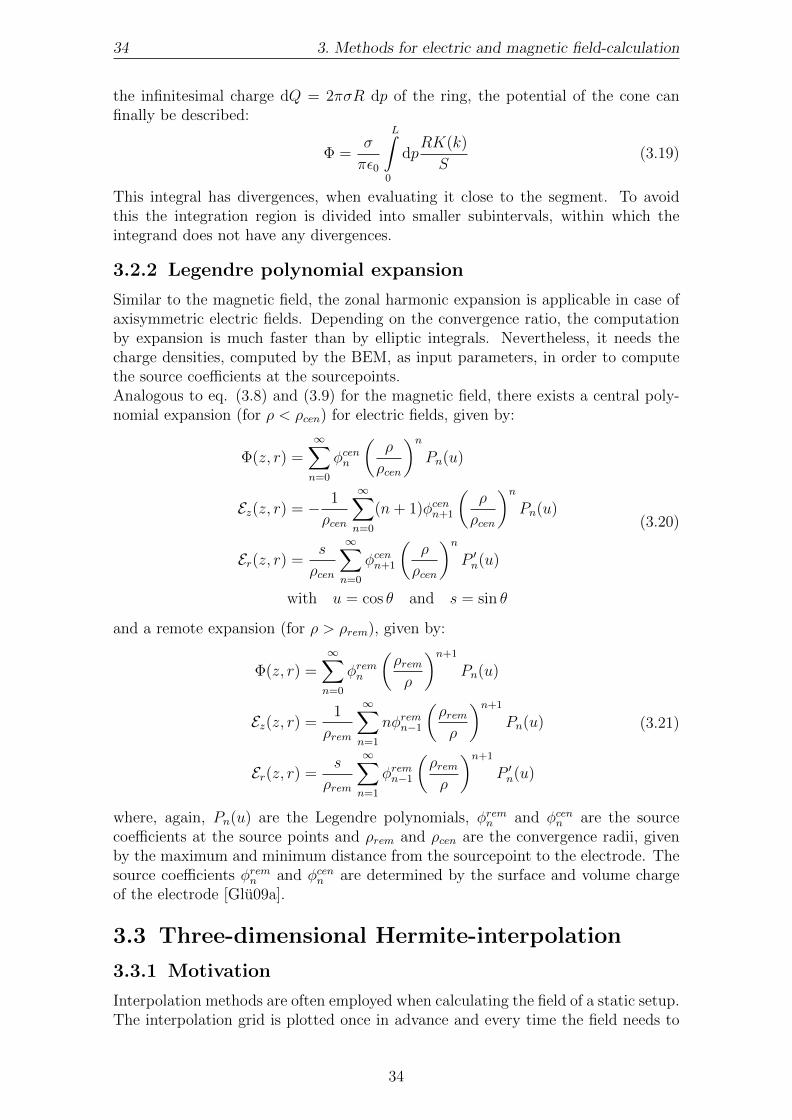
34 3. Methods for electric and magnetic field-calculation
the infinitesimal charge dQ = 2πσR dp of the ring, the potential of the cone canfinally be described:
Φ =σ
πε0
L∫0
dpRK(k)
S(3.19)
This integral has divergences, when evaluating it close to the segment. To avoidthis the integration region is divided into smaller subintervals, within which theintegrand does not have any divergences.
3.2.2 Legendre polynomial expansion
Similar to the magnetic field, the zonal harmonic expansion is applicable in case ofaxisymmetric electric fields. Depending on the convergence ratio, the computationby expansion is much faster than by elliptic integrals. Nevertheless, it needs thecharge densities, computed by the BEM, as input parameters, in order to computethe source coefficients at the sourcepoints.Analogous to eq. (3.8) and (3.9) for the magnetic field, there exists a central poly-nomial expansion (for ρ < ρcen) for electric fields, given by:
Φ(z, r) =∞∑n=0
φcenn
(ρ
ρcen
)nPn(u)
Ez(z, r) = − 1
ρcen
∞∑n=0
(n+ 1)φcenn+1
(ρ
ρcen
)nPn(u)
Er(z, r) =s
ρcen
∞∑n=0
φcenn+1
(ρ
ρcen
)nP ′n(u)
with u = cos θ and s = sin θ
(3.20)
and a remote expansion (for ρ > ρrem), given by:
Φ(z, r) =∞∑n=0
φremn
(ρremρ
)n+1
Pn(u)
Ez(z, r) =1
ρrem
∞∑n=1
nφremn−1
(ρremρ
)n+1
Pn(u)
Er(z, r) =s
ρrem
∞∑n=1
φremn−1
(ρremρ
)n+1
P ′n(u)
(3.21)
where, again, Pn(u) are the Legendre polynomials, φremn and φcenn are the sourcecoefficients at the source points and ρrem and ρcen are the convergence radii, givenby the maximum and minimum distance from the sourcepoint to the electrode. Thesource coefficients φremn and φcenn are determined by the surface and volume chargeof the electrode [Glu09a].
3.3 Three-dimensional Hermite-interpolation
3.3.1 Motivation
Interpolation methods are often employed when calculating the field of a static setup.The interpolation grid is plotted once in advance and every time the field needs to
34

3.3. Three-dimensional Hermite-interpolation 35
be evaluated in a certain point, it is interpolated and optionally scaled using theprecomputed grid. The Hermite-interpolation, in contrast to the linear-interpolationdoes not only need the values at the grid points, but also their partial derivates.This results in a longer precomputation time, but as the accuracy of the Hermite-interpolation scales not just with the 2nd but with the 4th power of the grid distance,this is the preferred method to use when interpolating with relatively large grids.Interpolating usually means a dramatic speed up of the field calculations, especiallyfor non axisymmetric fields and still grants a high numeric precision. However, inaxisymmetric fields, close to the symmetry axis, the Legendre-polynomial methodsare faster.
3.3.2 Theory
Q
1
2
6
5 8
7
3
4
x1
x2
x3
We are given a rectangular, three-dimensional grid that consists of cuboids. A cuboidQ of this grid can be described as follows.
Q :=
(x1, x2, x3) ε R3 / xui < xi < xoi ; i = 1, 2, 3
(3.22)
Through a coordinate-transformation of the form:
ui =xi − xmi
aiwith
xmi =xoi + xui
2and ai =
xoi − xui2
(3.23)
we project Q to the unit-cube E:
E :=
(u1, u2, u3) ε R3 / − 1 < ui < 1 ; i = 1, 2, 3
(3.24)
Now we define a function g(~u) on E with:
f(~x) = g(~u(~x)) (3.25)
The goal is to interpolate g(~u) within the unit-cube E. Therefore, we need toknow the function-values at the eight corner points ~ui as well as their first partialderivatives. We combine them into a Matrix G, where the function-values fill onecolumn:
Gi0 := g(~ui) (i = 1, ..., 8) (3.26)
35

36 3. Methods for electric and magnetic field-calculation
and the others are filled by their partial derivatives:
Gij :=
∂g(~u)
∂uj
~u=~ui
(i = 1, ..., 8 ; j = 1, 2, 3) (3.27)
The next step is to define a so called Interpolation-polynomial:
G(~u) =8∑i=1
3∑j=0
Gijφij(~u) (3.28)
The coefficient-polynomials φij are chosen, so that G(~uk) = Gk0 and∂g(~u)∂u1
~u=~uk
= Gk1. This leads to the following constraints:
φij(~uk) = δikδj0 and
∂φij(~u)
∂u1
~u=~uk
= δikδj1 (3.29)
These are fulfilled, if we define φij like:
φij(~u) := uij
3∏k=1
ϕjk(uik · ~uk) (3.30)
where ϕjk is given by:
ϕjk(t) :=1
4
[(2 + 3t− t3
)+(−3− 4t+ t2 + 2t3
)δjk]
and ui0 := 1 (3.31)
In order to interpolate the function f(~x) within the cuboid Q, we have to followsome simple steps:
1. calculate the function-values and their partial derivatives of f regarding ~x atall 8 corner points,
2. transform them into the unit-cube E:
Gij =
aj ·∂f(~x)∂xj
~x=~xi
if j > 0
f(~xi) if j = 0(3.32)
3. and interpolate function-values and derivatives at any point ~x ε Q :
∂f(~x)
∂xj= a−1
j ·∂G(~u(~x))
∂ujj = 1, 2, 3
f(~x) = G(~u(~x))
(3.33)
Interpolation methods yield the possibility of a scalable precision. When a highprecision is needed, the distance between the grid points can be chosen very smalland in the contrary case, when a lower precision is sufficient, it can be chosen ratherlarge. This has no impact on the actual computation time, just on the time neededto compute the initial grid.
36

4. Tracking of charged particles
This chapter describes the mathematical methods and approximations that are usedto calculate the trajectories of charged particles in the KATRIN experiment. At first,the Runge-Kutta methods will be introduced, which are able to approximate thesolutions of 1st order differential equation systems. This is followed by descriptions,how this numerical solvers can be applied to calculate particle trajectories and fieldlines. The chapter concludes with a rather simple example of how to calculaterelative distances of a particle to geometry components.
4.1 The Runge-Kutta method
The Runge-Kutta methods are a family of implicit and explicit iterative methods forthe approximation of solutions of ordinary differential equations. They have proventhemselves to have a very high precision. In this section, a brief introduction to theexplicit 4th order Runge-Kutta (RK4) will be given. Although both the 4th orderand 8th order Runge-Kutta methods are being used for particle tracking calcula-tions in the KATRIN experiment, this section will just describe the RK4 methodin detail. Conclusively, there will be a short description of the generalization of theRK4 method to higher orders.
The basic idea of the RK methods is the same as for the Euler method: An ex-act solution y = y(x) of a 1st order ordinary differential equation
y′ = f(x; y) (4.1)
with the given initial value y(x0) = y0 is replaced by a line in every sub-interval oflength h.The starting point is the given initial point P0 = (x0; y0). We replace the solutionwithin the interval x0 ≤ x ≤ x1 with a line that is descibed by the equation:
y − y0
x− x0
= m or y = y0 + (x− x0)m (4.2)
37

38 4. Tracking of charged particles
In contrast to the Euler method1, the slope m of the replacement-line is takenas a weighted average of slopes of the solution, taking into account: the slope atthe beginning of the interval: (k1); two mutually distinct computed slopes at themidpoint of the interval: (k2,k3); and the slope at the end of the interval: (k4). Withthese the approximated solution y(x), running through Pn(xn; yn) can be computedpoint-wise:
y(xn+1) ≈ yn+1 = yn +1
6(k1 + 2k2 + 2k3 + k4) with
k1 = h · f(xn; yn)
k2 = h · f(xn +
h
2; yn +
k1
2
)k3 = h · f
(xn +
h
2; yn +
k2
2
)k4 = h · f(xn + h; yn + k3)
(4.3)
The auxiliary quantities k1, k2, k3 and k4 have to be computed for every step. Theerror of the method estimates to:
∆yk = y(xk)− yk ≈1
15(yk − yk), (4.4)
where y(xk) is the exact solution at xk, yk the approximate solution at xk with step-size h and yk the approximate solution at xk with doubled step-size 2h.
yn
1
2
3
4
yn+1
Figure 4.1: Graphical interpretation of the 4th order Runge-Kutta method. In eachstep the derivative is evaluated four times: once at the initial point, twiceat trial midpoints, and once at a trial endpoint. From these derivativesthe final function value (filled dot) is calculated. Figure taken from[PTVF07]
The generalization for the approximate solution, taking into account s derivatives,is given by [Pap96]:
y(xn+1) ≈ yn+1 = yn + hs∑i=1
biki (4.5)
1In the Euler method, only the slope in the left boundary point of the interval is taken intoaccount.
38

4.2. Particle motion in general force fields 39
with the auxiliary quantities ki described by:
ki = f
(xn + hci;h
s∑j=1
aijkj
). (4.6)
The coefficients bi, ci and aij are given through the so called Butcher-tables [Ver78].Although the RK8 method needs 13 computation steps and the RK4 only 4, RK8is the preferred method because the step size h can be chosen larger than RK4with equal numerical precision. Clever use of this advantage makes the computationabout 10 times faster for RK8 than for RK4.
4.2 Particle motion in general force fields
This section gives an example, how to apply the Runge-Kutta method to a physicalproblem. Given is a non-relativistic particle that is moving in a general force fieldand we aim to calculate its trajectory.The motion of a particle in such a field can be written as a 1st order differentialequation system:
xj = vj
vj =1
mFj(x1, x2, x3; v1, v2, v3; t) (j = 1, 2, 3)
(4.7)
where x1, x2, x3 are the Cartesian space coordinates, v1, v2, v3 are the componentsof the particle’s velocity, t is the time, m is the mass of the particle and Fj are theforces acting on it. The differential equation system (4.7) consists of 6 first orderdifferential equations. The yi variables (i = 1, .., 6) are defined as:
yi = xi for i = 1, 2, 3 and
yi = vi−3 for i = 4, 5, 6.(4.8)
Equation (4.7) can now be expressed in terms of the derivative function f :
f(i, y1, ..., y6, t) = vi for i = 1, 2, 3 and
f(i, y1, ..., y6, t) =1
mFi−3 for i = 3, 4, 5.
(4.9)
With these, we are now able to calculate the trajectory of the particle via Runge-Kutta-steps.
4.3 Charged particle motion in electric and mag-
netic fields
For the KATRIN experiment, the trajectories of relativistic electrons are of maininterest. Therefore a way to compute the electron-trajectories within electric andmagnetic fields is very important.A particle in an electro-magnetic field is experiencing the Lorentz-force:
~FL = q(~E + ~v × ~B
)(4.10)
39

40 4. Tracking of charged particles
with q being the charge of the particle, ~v the velocity 3-vector, ~E the electric fieldvector and the ~B magnetic field vector.Again, we can write down a first order differential equation system, describing themotion:
~x = ~v and
~p = ~FL,(4.11)
where ~v and ~p are the velocity and momentum 3-vectors. In this case the yi variablesare defined by the momentum instead of the velocity:
yi = xi for i = 1, 2, 3 and
yi = pi−3 for i = 4, 5, 6.(4.12)
For the KATRIN electrons we use the relativistic relations between velocity andmomentum:
~p =m~v√1− ~v2
c2
and
~v =~p√
m2 + ~p2
c2
,
(4.13)
where m stands for the rest mass. Then the derivate functions are:
f(i, y1, ..., y6, t) = vi for i = 1, 2, 3 and
f(i, y1, ..., y6, t) =1
mFL,i−3 for i = 4, 5, 6.
(4.14)
with vi being calculated using the relations from the equations (4.13). For furtherinformation see [Glu02].
4.4 Field lines
When speaking of the motion of charged particles, field lines might not be the firstthing that comes to mind. In fact, calculation of field lines and calculation of particletrajectories are very related to each other, as they are both defined by a specific force.
In general, the calculation of field lines is a very important task in electro-magneticsimulations. It is essential when studying new electrode designs to, for example,control the electric potential along a magnetic field line in order to avoid penningtraps. It is even possible to approximate the actual electron trajectory with a fieldline, as the electrons perform a cyclotron motion around those field lines, thus savingcomputation time.
The differential equation system defining a field line of a three-dimensional vectorfield ~A is:
dxids
= ± Ai| ~A|
(i = 1, 2, 3). (4.15)
with s denoting the path. This equation system is time independent. Instead ofa force that depends on location and velocity, the “force“ in the case of field lines
40

4.5. Adiabatic approximation 41
just depends on the position. As usual, we define yi variables for the Runge-Kuttamethod:
yi = xi for i = 1, 2, 3, (4.16)
and the derivative functions f , which embed the ”force“:
f(i, y1, y2, y3, t) = ± Ai| ~A|
for i = 1, 2, 3. (4.17)
As the initial differential equation system (4.15) has only 3 components, the compu-tation of field lines is pretty fast. By slightly modifying the ”force“, so that it pointsorthogonal to field vector, it is also possible to compute equipotential lines.
4.5 Adiabatic approximation
Charged particles flying through a time- and position-independent magnetic fieldperform a uniform cyclotron motion. It can be described by a circular motion withits center moving along the magnetic field lines. If the magnetic field is in factdependent on time or position there is no longer an ideal cyclotron motion, but is isassumed as an approximately cyclotron-like motion. The basic idea of the adiabaticapproximation is that the actual motion can be approximated by taking the idealmotion and adding some corrections to it.At first the motion of the center of the cyclotron motion, the so called guidingcentre motion shall be described. It is very similar to the field lines and given bythe differential equation system:
~x =Bi
| ~B|v‖ and
p‖ = −µγ~∇‖ ~B + qE‖,
(4.18)
where µ =p2⊥
2m| ~B| is the magnetic moment, γ =
√1 +
p2‖+p2⊥
m2c2the Lorentz-factor and
E‖ the electric field parallel to the magnetic field ~B. The velocity v‖, the momentump‖ and the gradient ∇‖ are parallel to the magnetic field as well.The yi variables are then defined as follows:
yi = xi for i = 1, 2, 3 and
yi = p‖ for i = 4.(4.19)
The derivative functions are again obtained by the force:
f(i, y1, ..., y4, t) =Bi
| ~B|v‖ for i = 1, 2, 3 and
f(i, y1, ..., y4, t) = −µγ~∇‖ ~B + qE‖ for i = 4.
(4.20)
The guiding centre performs a longitudinal motion along the magnetic field lines. Toapproximate the real cyclotron motion, a motion transversal to the magnetic fieldlines has to be added.
41

42 4. Tracking of charged particles
With the adiabatic invariant µ = γ+12
E⊥| ~B| (see section 2.3.2) and the transversal
momentum p⊥ = 2µm| ~B| the cyclotron radius can be expressed by:
r =γmv⊥
q| ~B|=
p⊥
q| ~B|(4.21)
With the given step size of the Runge-Kutta step h and the cyclotron frequency
ω = q| ~B|mγ
, the change of the azimuthal angle results to:
∆ϕ = ωh (4.22)
The cyclotron radius and the change of azimuthal angle completely describe theapproximated transversal motion. They are simply added to the guiding centre po-sition at the end of the Runge-Kutta step, resulting in an adiabatic approximatedstep.This approximation has proven itself to be very fast if the step size h is large. Forsmall step sizes h and especially when tracking close to an electrode, this approxi-mation is often slower than the ”exact” numerical solution, because it requires moreelectric field calculations, which are rather slow. The step size is controlled by mon-itoring the energy conservation. If the energy conservation within one step is notgood enough, the step size is reduced and the step is redone. If it is sufficient, thestep size for the next step is increased.A gyrating electron performs an additional magnetron motion. This magnetron drifthas also to be added separately to the step, for further informations see [Thu02].
4.6 Distance calculation
In order to decide which field calculation method to use during particle trackingand when investigating if a particle hits a certain geometrical object, it is crucial toknow the distance between the particle and the geometrical components. This allowsdynamic switching between field calculation methods and trajectory monitoring andcontrol, depending on this distance.Nearly all geometries to which we want to check the distance can be approximatedby cones. Therefore, we can simplify the task of distance monitoring, to distancecalculations to various cones forming the geometry. Figure 4.2 shows a general conedescribed by two points (~a1,~a2) and two radii (r1,r2).First, we calculate the ”orientation“ vector ~n of the cone:
~n =~a2 − ~a1
|~a2 − ~a1|, (4.23)
It describes the orientation of the two boundary planes of the cone. For the specialcase of a disc (~a1 = ~a2) this vector must be specified. The next step is projecting ~xito the symmetry axis of the cone:
~x′i = ~a1 + [~n · (~xi − ~a1)]~n. (4.24)
With ~x′i it is already possible to check if the point ~xi lies within the volume definedby the cone surface (|~x′i−~aj| ≷ |~a1−~a2|). Now we build a unity vector pointing into
42

4.6. Distance calculation 43
r1
r2
~a1 ~a2
~x1
~x2
Figure 4.2: Illustration of a cone, represented by two the vectors pointing to thestart- and endpoint of the cone on its symmetry axis ~a1 and ~a2, and tworadii at these points r1 and r2. The distance shall be calculated for apoint outside the cone (~x1) and a point inside the cone (~x2).
the direction from ~x′i to ~xi and project it onto the edges of the cone. This definestwo points ~α1 and ~α2 on the cone edges:
~αj = ~aj + rj~xi − ~x′i|~xi − ~x′i|
. (4.25)
In the case of point ~x1 that lies outside of the cone, the distance is obtained by justcalculating
dj = |~αj − ~x1|, (4.26)
and searching for the minimum. For ~x2 we need to calculate another auxiliary vector~β that lies on the line, linking two points on the cone edges, ~α1 and ~α2:
~β = ~α1 +
[~α2 − ~α1
|~α2 − ~α1|(~x2 − ~α1)
]~α2 − ~α1
|~α2 − ~α1|. (4.27)
The requested distance d is then given by:
d = |~x2 − ~β| (4.28)
In order to save computation time this computation chain is executed up to equation(4.26) and then just the distances to the cones within as sphere, defined by εd arecomputed further.
43


5. Code implementation
This chapter deals with the implementation of the calculation methods introducedin the chapters 3 and 4 into a C++ framework. Several of them existed already inC-code [Glu06]. In context of this diploma thesis, together with S. Mertens and withcontributions of N. Wandkowsky, they were reworked and rewritten into a more tech-nically sophisticated form, in order to be standardised, flexible, modular and easyto use. The novel implementations of the line-segment and interpolation methodsform the KNAXS (KATRIN Non-AXisymmetric field Simulation) field calculationpackage. The following chapter is not a line per line programme documentation buta basic description of the classes and how they work. The source-code is fully avail-able from the KATRIN-subversion-repository [rep]. The whole code is now part ofthe Kassiopeia framework that aims to be a universal tool for a complete physicalsimulation of the KATRIN experiment. It includes the simulation of the source, es-pecially gas dynamics and particle generation, field calculation and particle trackingand simulation of detector and data-aquisition [Obl].
5.1 Overview
Figure 5.1 shows an overview of the KTrack framework. It is able to track chargedparticles within almost the whole KATRIN experiment, and can, in addition, com-pute electric and magnetic field lines of specified fields.The framework features a management structure, consisting of the following classes:
• Initializer: it reads in the major configuration file, creates and configuresall other objects that are needed for trajectory calculation.
• ExitConditionChecker: this class monitors the particle being tracked andchecks if any exit conditions for the track are reached, like, for example, theparticle leaving the area of interest or hitting a wall etc.
• TrackOutput: this class manages the output of the programme. It writes userconfigured information about the track into an output file.
The physics component classes are independent and, though being created by theInitializer during runtime, not members of the KTrack framework, except for the
45

46 5. Code implementation
Figure 5.1: Overview of the KTrack program package. Shown is the structure thatdivides into the management classes (orange), the physics classes (green)including the external field classes and the core components (blue), re-sponsible for the trajectory calculation.
KTrackParticle. The KTrackParticle describes not only the physical attributesof a particle, like mass and charge, but contains also some technical information likea label, a time stamp and other track information. The field classes will be discussedin more detail in the following section 5.2.The core component classes work together in order to perform the actual tracking.They are discussed in detail in section 5.3.
5.2 Field classes
The field classes in the Kassiopeia programme package have to be compatible andusable by a lot of other classes and programmes. Because of this, two abstract baseclasses were defined, Elfield and Magfield, and every electric and magnetic fieldclass must inherit from them.
Listing 5.1 shows the source code of the Elfield base class. It uses TVector3, aclass from the ROOT programme package [ROO] that represents a three-dimensionalvector. The two virtual methods GetField and GetPhi are pure and have to beredefined by every derived class. They are the key interface to obtain the electricfield and potential.
46

5.2. Field classes 47
Listing 5.1: The header Elfield.h that describes the abstract class Elfield
class E l f i e l d
public :E l f i e l d ( )
virtual ˜ E l f i e l d ( ) virtual TVector3 GetFie ld ( const TVector3& p) = 0 ;virtual double GetPhi ( const TVector3& p) = 0 ;
;
Listing 5.1: The header Elfield.h that describes the abstract class Elfield
Listing 5.2 shows the source code of the Magfield base class. It is very similar to theElfield class and uses also the TVector3 class from ROOT. Magfield has the pure,virtual method GetField that has to be redefined in every derived class analogouslyto Elfield it returns the magnetic field at the field point specified by the Tvector3
p.
Listing 5.2: The header Magfield.h that describes the abstract class Magfield
class Magf ie ld
public :Magf ie ld ( )
virtual ˜ Magf ie ld ( ) virtual TVector3 GetFie ld ( const TVector3& p) = 0 ;
;
Listing 5.2: The header Magfield.h that describes the abstract class Magfield
5.2.1 Magfield3
Magfield3 is basesdon the magfield3.c C-program [Glu06]. It calculates the mag-netic field by using the elliptic integrals or the Legendre polynomial expansion (seesection 3.1.2). It is also capable of magnetic field calculations for a coil system withdifferent axial symmetry axes.The input-file describing the coil setup does have the following structure:
N
J[1] A[1][x-z] B[1][x-z] Rmin[1] Rmax[1] n[1]...
......
......
......
......
...J[N] A[N][x-z] B[N][x-z] Rmin[N] Rmax[N] n[N]
with N being the number of coils described in the setup, J[i] being the currentdensity in the coil, A[i][x-z] and B[i][x-z] being the coordinates of the coil endpoints, Rmin[i] and Rmax[i] being the inner and outer radii of the coil and n[i]
being the number of subsegments the coil is divided into for numerical integration.These parameters are all given in SI-units.
47

48 5. Code implementation
Prior to the magnetic field computation, Magfield3 tests the input coils and writesthem, with additional information, in a file (extension .magcoil3). Then it computesthe central and remote source points and coefficients for the coil system, and storesthem in separate files that are either specified by the user or chosen automatically.These files carry the extensions .magsource3_central and .magsource3_remote
respectively. The source points and coefficients for all coils with the global axisas symmetry axis are evaluated separately and stored in a file with the extension.magsource3_axisymm. This last step is not essential, but it offers the opportunityto save computation time, because the Legendre polynomial expansion of these coilcan be combined to one.After these preparing computations, the field at a point, defined by the TVector3
position, is obtained with the GetField(position) method. Depending on thedistance from the field point to the coils and the symmetry axis, the method chooseseither the Legendre polynomial expansion method or the elliptic integrals to computethe magnetic field.
5.2.2 Elfield2
The Elfield2 class is based on the C-program elcd2.c [Glu06]. It is able to com-pute the electric potential and field of an electrode system that consists of solid,axially symmetric electrodes using the field computation methods introduced in sec-tion 3.2. The class is not able to compute the field and potential of wires present inthe geometry directly, but they have to be approximated by solid cones. The inputfiles the extension .el2 and are of the following structure:
N
g[1] Z1[1] R1[1] Z2[1] R2[1] U[1] n[1]...
......
......
......
g[N] Z1[N] R1[N] Z2[N] R2[N] U[N] n[N]
N specifies the number of electrodes in the file. g[i] denotes the group index, Z1[i],R1[i] and Z2[i], R2[i] are the cylindrical coordinates of the cone edges, U[i] thevoltages of the cones and n[i] the number of conical subelements, a cone is dividedin for numerical integration. Again all physical quantities are given in SI-units.The class has to perform three steps in advance as preparation, in order to be ableto compute the electric field and potential:
1. Discretization of the full electrodes into many small subelements. They aresaved in a file with the extension .element2.
2. Calculation of the charge densities within the subelements, using the boundaryelement method.
3. Calculation of the source coefficients at the source points. They are written ina file with the extension .elsource2.
With these steps done the class is now able to calculate the electric field and po-tential. As it inherits from the abstract base class Elfield, the virtual method Get-
Field(position) returns the electric field, and the virtual method GetPhi(position)
the electric potential, at any field point specified by the TVector3 position for
48

5.2. Field classes 49
which the field calculation methods are valid. The class decides automatically whichmethod to to use, elliptic integrals or Legendre polynomial expansion, depending onthe convergence radii.
5.2.3 Elfield32
Elfield32 is an upgrade of the Elfield2 class is based on the C-program elcd3_2.c
[Glu06]. In addition to the calculation of the electric field and potential of fullelectrodes, it is also able to compute the electric field and potential of wire electrodesthat have a cylindrical symmetry with the centre on the z-axis. Therefire they haveto be approximated as linear segments. The input files for Elfield32 have theextension .el32. The input file for the full electrodes looks as following:
N
Z1[1] R1[1] Z2[1] R2[1] U[1] n[1]...
......
......
...Z1[N] R1[N] Z2[N] R2[N] U[N] n[N]
It is almost the same as for the Elfield2 class, except that the group index ismissing. Again, N specifies the number of electrodes in the file, Z1[i], R1[i] andZ2[i], R2[i] are the cylindrical coordinates of the cone edges, U[i] the voltagesof the cones and n[i] the number of conical subelements, a cone is divided into fornumerical integration.The wires are defined in a separate input file with the form :
N
Z1[1] R1[1] Z2[1] R2[1] d[1] phi[1] Numwire[1] U[1] n[1]...
......
......
......
...Z1[N] R1[N] Z2[N] R2[N] d[N] phi[N] Numwire[N] U[N] n[N]
N specifies the number of wire electrodes. The wires of a wire electrode lie on acone with startpoint Z1[i], R1[i] and endpoint Z2[i], R2[i] given in cylindricalcoordinates. The wire diameter d[i] in meter, their azimuthal angle phi[i] in degand their number Numwire[i] are specified additionally. Again, U[i] denotes thevoltage of the wires and n[i] the number of subelements the wires have to be di-vided into for numerical integration.Elfield32 has to do the same preparation calculation as Elfield2, with the differ-ence that the wire electrodes are represented by linear instead of conical segments.Analogously, a subelement file with the extension .element32 and a source coef-ficient file with the extension .elsource32 are created. Elfield32 also inheritsfrom the abstract base class Elfield, and thereby redefines the GetPhi and Get-
Field methods. Like Elfield2, it is able to switch between calculation of the fullelectrodes by elliptic integrals or Legendre polynomial expansion, depending on theposition of the field point.
5.2.4 Elfield33
The class Elfied33 is able to compute the electric potential and field of an arbitraryelectrode system, and is based on the C-program elcd3_3.c [Glu06]. However, the
49

50 5. Code implementation
r
z
z1, r1
z2, r2
ϕ
r
d
Figure 5.2: Graphical explanations of the electrode input parameters.
class is not able to do a discretization of the electrodes on its own. The user hasto do this in advance, and then pass the appropriate input file with the extension.el33 that contains the discretized electrode geometry to the method. The inputfile is of the form:
L
l[1] g[1] type[1] rot[1] P1-P11[1] U[1]...
......
......
...l[L] g[L] type[L] rot[L] P1-P11[L] U[L]
L specifies the number of lines in the file, and thereby the number of subelements,l[i] are the subelement indices and g[i] the subelement-group indices, which arethe same for subelements with the same charge density. type[i] are integers thatdetermine the type of the subelements: for type[i]=1 the subelement is a rectangleand for type[i]=2 it is a wire. The integers rot[i] define the rotational number, ifthey are greater than 1, rot[i]-1 extra subelements are added. They are obtainedby discrete rotational transformations of the given subelements along the z-axis,forming a uniform azimuthal distribution. The values of type[i] and rot[i] shouldbe the same for every subelement in a group g[i]. The eleven parameters P1-P11[i]define the geometry of the subelements. For rectangles (type[i]=1) they have thefollowing definition (see figure 5.3):
• P1-P3[i] are the three Cartesian coordinates of a corner point P0 of the rect-angles
• P4-P6[i] are the components of the unit vector ~n1 that points from P0 towardsthe neighbouring corner point P1
• P7-P9[i] are the components of the unit vector ~n2 that points from P0 to-wards the other neighbouring corner point P2, the vectors ~n1 and ~n2 should beorthonormal
• P10[i] are the edge lengths a of the rectangles corresponding to ~n1
• P11[i] are the edge lengths b of the rectangles corresponding to ~n2
50

5.2. Field classes 51
As for wires (type[i]=2), they have the definitions:
• P1-P3[i] are the three Cartesian coordinates of one endpoint Pa of the wires
• P4-P6[i] are the three Cartesian coordinates of the other endpoint Pb of thewires
• P7[i] are the diameters d of the wires
• P8-P11[i] are not used, but must be filled with arbitrary numbers, in case ofwires
U[i] contains the voltages of the subelements.
P0
P2
P1
a
b
~n1
~n2 Pa Pb
d
Figure 5.3: Geometrical parameter definition of a rectangular (left) and a wire (right)subelement.
After the subelements are read in, the corresponding charge densities are calculatedvia a Gauss-Jordan-algorithm using their voltage values. The subelements and theircharge densities are written into a file with the extension .element33. With allpreparations done, the Elfield33 class is able to calculate the electric potentialand field of the given geometry by numerical integration. Similar to all electric fieldclasses, it inherits from the abstract base class Elfield, redefining the GetPhi andGetField methods. The field and potential calculations in Elfield33 are ratherslow, compared to other electric field calculation classes. This is due to the fact thatthe fast Legendre polynomial expansion can only be used with axially symmetricelectrode setups. On the other hand, Elfield33 has the advantage that it can copewith all kinds of (discretized) electrode geometries.
5.2.5 BiotSavart
This class is an implementation of the integrated Biot-Savart method introduced insection 3.1.1.1. Figure 5.4 shows a diagram of the class.BiotSavart uses line-current segments with which the geometry is approximated,and calculates their resulting magnetic field. It is possible to read in input lines froma file and/or create and add Line objects dynamically during runtime. The inputfile, with the extension .bio, has the form:
X1[0] Y1[0] Z1[0] X2[0] Y2[0] Z2[0] I[0]...
......
......
......
X1[N] Y1[N] Z1[N] X2[N] Y2[N] Z2[N] I[N]
51

52 5. Code implementation
Figure 5.4: Overview of the Biot-Savart class: It inherits from Magfield and hasone or more member objects of the class Line.
where X1-Z1[i] and X2-Z2[i] are the Cartesian coordinates of the start and end-point and I[i] is the current in the line segment, flowing from the start- to theendpoint. So, every row describes one Line object that is added to the BiotSavart
object. As it inherits from the abstract class Magfield, the field at the field pointTVector3 position can be obtained by the virtual method GetField(position).
5.2.6 MagMaterials
The MagMaterials class calculates the magnetic field of dipole-bars, as described insection 3.1.1.2. Figure 5.5 shows a principle diagram of the class.The dipole-bars are described by Bar objects, which can, analogously to the Biot-
savart class, be read in from an input file and/or created and added during runtime.The input files use the extension .magmat and contain data with the following for-mat:
X1[0] Y1[0] Z1[0] X2[0] Y2[0] Z2[0] M[0] R[0] Chi[0]...
......
......
......
......
X1[N] Y1[N] Z1[N] X2[N] Y2[N] Z2[N] M[N] R[N] Chi[N]
A Bar object is described by: the Cartesian coordinates of its start- and endpointX1-Z1[i] and X2-Z2[i], the strength of the magnetisation pointing from the start-to the endpoint M[i], the radius of the bar R[i] and the magnetic susceptibilityChi[i] of the bar material. As for all classes, derived from Magfield, the field canbe obtained with the GetField method.
52

5.2. Field classes 53
Figure 5.5: Overview of the MagMaterials class: It inherits from Magfield and hasone or more member objects of the class Bar.
5.2.7 Interpolation
In section 3.3 we learned about using the three-dimensional Hermite-interpolationto speed up field calculations. This method was implemented in a very modulardesign into the class FieldInterpolation. The classes MagfieldInterpolate andElfieldInterpolate inherit from this class, and of course from the abstract fieldbase classes. Figure 5.6 shows a principle diagram of the MagfieldInterpolate
class and figure 5.7 of the ElfieldInterpolate class, respectively.Objects of the stereotype FieldInterpolation store one or more interpolation gridsin objects of the stereotype Fieldmap. These grids contain for example the scalarelectric potential with just one value at a grid point in case of a Fieldmap1 object,and the grids for the three-dimensional vector fields, that have three values and ninepartial derivatives in one grid point, are stored in Fieldmap3 objects. In case ofrotational symmetry, one can also use the Fieldmap2 objects, but this has to bespecified explicitly by the user.In order to pre-compute a grid, the virtual methods CreateMagFieldmap and Cre-
ateElFieldmap that are members of the Fieldmap classes have to be called. Theycompute a grid of the specified Magfield or Elfield object, respectively. Cre-
ateElfieldmap actually creates two field maps, one for the electric field and onefor the potential. Afterwards they are saved to a file and can be read in with thevirtual method ReadMapFromFile. For the Fieldmap1 classes, the grid points arestored into files of the form:
53
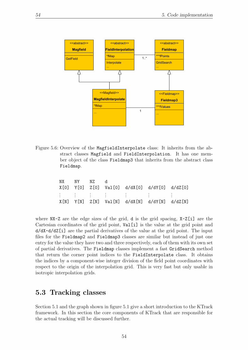
54 5. Code implementation
Figure 5.6: Overview of the MagfieldInterpolate class: It inherits from the ab-stract classes Magfield and FieldInterpolation. It has one mem-ber object of the class Fieldmap3 that inherits from the abstract classFieldmap.
NX NY NZ d
X[0] Y[0] Z[0] Val[0] d/dX[0] d/dY[0] d/dZ[0]...
......
......
......
X[N] Y[N] Z[N] Val[N] d/dX[N] d/dY[N] d/dZ[N]
where NX-Z are the edge sizes of the grid, d is the grid spacing, X-Z[i] are theCartesian coordinates of the grid point, Val[i] is the value at the grid point andd/dX-d/dZ[i] are the partial derivatives of the value at the grid point. The inputfiles for the Fieldmap2 and Fieldmap3 classes are similar but instead of just oneentry for the value they have two and three respectively, each of them with its own setof partial derivatives. The Fieldmap classes implement a fast GridSearch methodthat return the corner point indices to the FieldInterpolate class. It obtainsthe indices by a component-wise integer division of the field point coordinates withrespect to the origin of the interpolation grid. This is very fast but only usable inisotropic interpolation grids.
5.3 Tracking classes
Section 5.1 and the graph shown in figure 5.1 give a short introduction to the KTrackframework. In this section the core components of KTrack that are responsible forthe actual tracking will be discussed further.
54

5.3. Tracking classes 55
Figure 5.7: Overview of the ElfieldInterpolate class: It inherits from the ab-stract classes Elfield and FieldInterpolation. It has two memberobjects that inherit from the abstract class Fieldmap: a Fieldmap1 ob-ject, in which the interpolation grid for the electric potential is storedand a Fieldmap2 or Fieldmap3 object, depending if the field is axiallysymmetric, in which the interpolation grid for the electric field is stored.
5.3.1 KTrackParticle
The class KTrackParticle is a virtual analogue to a physical particle, and has thesame basic attributes: charge, mass, position and momentum. To save computationtime, the class has extensive attributes like: kinetic energy, polar and azimuthal an-gles, Θ and ϕ, to the magnetic field, velocity, kinetic energy and their correspondinglongitudinal and transversal components, Lorentz-factor, etc. Altogether, there are28 additional parameters to the 4 that are needed to uniquely describe a particle.Some of them are derived physical quantities and some of them are technical quan-tities, like the particle-label or the total path length travelled by the particle duringtracking. The physical attributes of the KTrackParticle can be retrieved and al-tered by Get.. and Set.. methods. After setting an attribute, the Update methodhas to be called to guarantee consistency of the particle’s physical attributes. TheKTrackParticle also stores information about scattering processes that could havehappened during the track.
5.3.2 StepSize
StepSize is an abstract base class. The derived classes implement two virtual func-tions: ComputeTimeStep that returns the step size h for the next tracking step andCheck which tests the last tracking step and returns a boolean if valid (true) or not(false). At the moment, there are three other classes that implement the StepSizeclass:
55

56 5. Code implementation
• StepSizeFix: A trivial implementation that always returns a constant stepsize. The step size is defined in the constructor of the class. It is the only stepdetermination method functional without any magnetic field.
• StepSizeCyclotron: This class returns a fraction of the duration of one cy-clotron period at the particle’s current location. The fraction and global upperand lower limits for the step size are defined in the constructor of the class.
• StepSizeEnergy: This class should only be used, when using the adiabaticapproximation. It calculates the particle’s kinetic energy before and after thestep. If the energy conservation lies within user-defined limits, the step is validand the step size for the next step is increased up to the step size limit. If theenergy conservation is not below the upper limit, the step size is reduced andthe step is redone. The energy conservation and step size limits are specifiedin the constructor of the class.
In contrast to other components of the step computation mechanism, StepSizeCy-clotron and StepSizeEnergy are not usable for other purposes than for tracking.For other tasks that require the numerical solution of differential equation systems,for example field line calculation, only StepSizeFix can be used.
5.3.3 DiffEqSolver
All of the numerical solvers for differnetial equation systems implement the abstractDiffEqSolver class. The class has the virtual member function Solve. The stepsize h, the initial conditions yi and the ODE1 object, which simply computes thederivative functions fi, are passed to this function. It returns a vector<double>
in which the final conditions are stored. At the moment three classes exist thatimplement these base class: RungeKutta4 and RungeKutta8 which are 4th and 8therror order implementations of the Runge-Kutta method introduced in section 4.1,and the experimental PredictorCorrector class that uses the Predictor-Correctormethod to numerically solve first order differential equation systems [PTVF07].
5.3.4 StepComputer
The task of the StepComputer class is to manage the StepSize, ODE and DiffEq-
Solver objects and compute the attributes of the KTrackParticle at the locationof the next step. It also computes energy loss due to synchrotron radiation andchecks if scattering events occurred, calculates the attributes of the particle afterscattering and even creates secondary particles. StepComputer is an abstract baseclass and has just one interface, the virtual function MakeStep. The input for thismethod are the KtrackParticle to track and pointers of the type Elfield* andMagfield* to the polymorphic electric and magnetic field objects. With these itcomputes the step and writes its paramters into the KTrackParticle object. Thereare two classes implementing StepComputer:
• ExactStep: This step computer uses the “exact” numerical solution of theequation (4.10) to compute the step.
• ApproxStep: This step computer uses the adiabatic approximation describedin section 4.5.
1ODE stands for ordinary differential equation.
56

5.4. Comparison 57
To ensure the physical consistency of the KTrackParticle at any time during theruntime of the programme, the changes computed during the MakeStep call arestored in an intermediate particle. At the end of the step, this is then written intothe KTrackParticle object.
5.4 Comparison
The most important reasons for the creation of the KTrack and KNAXS programmepackages were:
• making the simulation tools more user friendly and simplify their structure
• improved flexibility by modular design
• equal or better precision and equal or faster computation speed
In order to evaluate, if these intentions were fulfilled, several computations were doneas comparison. Therefore, KTrack and KNAXS were compared with pre existing,software, if any, or, in case of the interpolation and line segment methods, comparedwith other field calculation methods.
5.4.1 Ktrack compared to singletraj.c
singletraj.c is a pre existing C-programme [Glu06], for fast tracking of particleswithin the pre- and main spectrometer. It uses magfield2.c to compute the mag-netic field and elcd2.c to compute the electric field and potential. Hence, onlyparticle tracks in axially symmetric systems can be computed, as magfield2.c doesnot support tilted coils.A track through the main spectrometer of an electron with 10 eV surplus energy tothe analysing potential was used for this comparison. The stepping parameters werethe same for both programmes and the positions of the particular steps agreed witha precision of 10−6 m for exact tracking and 10−4 m for adiabatic approximation.The track was run 10 times with every programme on an Intel Core 2 Quad Q6600with 4 GB of RAM and Ubuntu Linux 8.04 installed. The average values of theparticular computation times are listed in the tabular below:
KTrack singletraj.c
stepping type Exact Approx Exact Approxtime 4.5 s 1.5 s 10.6 s 2.5 s
This table clarifies two things: the adiabatic approximation normally just takes aquarter of the time of the exact computation and KTrack is nearly twice as fast assingletraj.c. The main reason for this is the consequent performance optimisationdone in the step computers and numerical solvers of KTrack. For example, all objectsare passed by reference, the memory is allocated dynamically and the routines weregenerally straightened.
57

58 5. Code implementation
5.4.2 Interpolation precision and computation time
In order to evaluate the possible fields of application for the field interpolationmethod, several test computations were done. In preparation, four particular in-terpolation grids were computed, with different grid spacings 1 mm, 5 mm, 10 mmand 50 mm. They were compared with the other field calculation methods that arecurrently implemented. As test 105 arbitrary points were chosen within the pre-spectrometer at which the particular fields were calculated. This ensures that fieldinterpolations in both, rather homogeneous and rather inhomogeneous regions aretaken into account. Field points at which some methods would not be able to com-pute the field, e.g. inside the coils or electrodes, were not used. The time for neededthe function call was recorded with the C-function clock() and averaged over allpoints. In addition, the relative errors of the fields magnitude and components, andin the case of electric fields, additionally the potential, were averaged.
MagfieldInterpolate vs. BiotSavartFor this test calculation, the field of a model of the EMCS with 672 line-elementswas calculated.
d [mm] t [s] tinterp [s] error errorx errory errorz1 6.112 e-04 1.720 e-05 3.74e-08 0 3.74e-08 05 4.160 e-04 5.000 e-06 5.03e-09 0 5.03e-09 0
10 4.230 e-04 2.000 e-06 2.70e-08 0 2.70e-08 050 4.110 e-04 1.100 e-05 5.75e-08 0 5.75e-08 0
Table 5.1: Computation time and error comparison between MagfieldInterpolate
and BiotSavart.
Table 5.1 and shows the results of the test. t denotes the average time for theGetField function call of BiotSavart and tinterp for MagfieldInterpolate, re-spectively. As expected, both times are independent of the grid spacing and theinterpolation is about ten to a hundred times faster than BiotSavart even with thisrelatively small number of line-elements to calculate. The relative error is shown forthe absolute magnetic field and the three field components. A 0 for the error means,that the numbers agree with double precision. Even for the largest grid-spacing of50 mm the error is in the order of 10−8 and thereby more than sufficient. For theinterpolation of the EMCS, the grid-spacing could be chosen even larger, to savememory and to shorten the computation time of the interpolation grid.
MagfieldInterpolate vs. MagMaterialsThe second test computation was the comparison of MagfieldInterpolate againstMagMaterials. The magnetic field of a model consisting of 2142 dipole bars wascomputed and interpolated within the main spectrometer.
Table 5.2 shows the results of this test computations. Again the computation timesof the interpolation are in the order of microseconds. And due to the many elementsto compute the MagMaterials class is 500 times slower. The relative errors are oneto two orders of magnitudes higher than for the interpolation of the EMCS. Thisis due to the stronger inhomogeneity of the field caused by the magnetic materials.
58

5.4. Comparison 59
d [mm] t [s] tinterp [s] error errorx errory errorz1 1.181 e-03 8.000 e-06 5.51e-07 5.63e-06 2.15e-05 2.72e-085 1.403 e-03 6.000 e-06 2.88e-06 2.82e-05 1.07e-04 1.39e-09
10 1.178 e-03 1.000 e-05 5.71e-06 5.65e-05 2.14e-04 4.02e-0850 1.175 e-03 9.000 e-06 2.86e-05 2.88e-04 1.06e-03 1.35e-08
Table 5.2: Computation time and error comparison between MagfieldInterpolate
and MagMaterials
However, even the error for 50 mm grid-spacing in the order of 10−5 is acceptable.With a fixed model of the magnetic dipole distribution in the experimental area, im-plying just one initial computation of the interpolation grid, MagfieldInterpolateis a significantly better choice for field computation.
MagfieldInterpolate vs. Magfield3 (Legendre polynomial)For this test the magnetic fields of all the coils in the KATRIN setup were computedinside the main spectrometer.
d [mm] t [s] tinterp [s] error errorx errory errorz1 8.100 e-06 1.270 e-05 4.34e-08 9.49e-03 0 4.34e-085 8.100 e-06 1.150 e-05 8.56e-08 4.73e-02 0 8.54e-08
10 8.800 e-06 1.220 e-05 4.32e-08 9.40e-02 0 4.34e-0850 7.000 e-06 1.300 e-05 2.35e-08 4.50e-01 0 2.19e-08
Table 5.3: Computation time and error comparison between MagfieldInterpolate
and Magfield3 (Legendre polynomial).
The results are shown in table 5.3. As expected, the Legendre polynomial expansionof the magnetic field is about twice as fast as the interpolation. The relative errorsare very small except for the x-component. In this case Magfield3 would be thebetter choice, as it is faster and the error of the x component would require a smallgrid-spacing.
MagfieldInterpolate vs. Magfield3 (elliptic integrals)Again, the magnetic fields of all the coils in the KATRIN setup were computed in-side the main spectrometer, but this time Magfield3 was forced to use the ellipticintegral field computation method.
d [mm] t [s] tinterp [s] error errorx errory errorz1 1.524 e-02 2.400 e-05 4.31e-08 9.49e-03 0 4.32e-085 1.413 e-02 2.100 e-05 8.65e-08 4.73e-02 0 8.64e-08
10 1.515 e-02 1.800 e-05 3.78e-08 9.40e-02 0 3.80e-0850 1.450 e-02 1.200 e-05 9.11e-09 4.50e-01 0 7.53e-09
Table 5.4: Computation time and error comparison between MagfieldInterpolate
and Magfield3 (elliptic).
59

60 5. Code implementation
The results are shown in table 5.4. The errors are in the very same order as for theLegendre polynomial expansion. And due to the time consuming numerical integra-tion, MagfieldInterpolate is nearly a thousand times faster than Magfield3 whenbeing forced to use the elliptic integral method. A computation method would bepossible, that combines the Legendre polynomial expansion that uses interpolationinstead of elliptic integrals in region where the expansions do not converge, thusgaining computation speed in these regions.
ElfieldInterpolate vs. Elfield2 (Legendre polynomial)For this test, the electric potential and field of the main spectrometer electrode setupwere calculated. As usual for computations with Elfield2, the wire electrodes wereapproximated by full electrodes.
d [mm] t [s] tinterp [s] error errorx errory errorz errorΦ
1 2.10 e-05 1.20 e-05 5.026e-08 0 0 2.384e-09 9.024e-085 1.30 e-05 1.00 e-05 1.277e-06 0 0 9.564e-08 9.024e-08
10 1.60 e-05 1.10 e-05 4.753e-06 0 0 1.073e-07 1.812e-0750 1.70 e-05 1.00 e-05 1.457e-04 0 0 4.568e-05 1.273e-07
Table 5.5: Computation time and error comparison between ElfieldInterpolate
and Elfield2 (Legendre polynomial).
Table 5.5 shows the results of this test computations. The polynomial expansion forthe electric field is insignificantly slower than for the magnetic field. The relativeerrors are very small and that of the x and y component are even better than doubleprecision for all grid-spacings. For this case no clear recommendation can be given,as the computation times are almost equal and the interpolation needs an extensivepreparation.
ElfieldInterpolate vs. Elfield2 (elliptic integrals)Again, the electric potential and field of the main spectrometer electrode setup werecalculated, but this time forcing Elfield2 to use the elliptic integral method.
d [mm] t [s] tinterp [s] error errorx errory errorz errorΦ
1 7.01 e-03 7.00 e-06 5.03e-08 0 0 2.38e-09 9.02e-085 7.00 e-03 1.20 e-05 1.28e-06 0 0 9.56e-08 9.02e-08
10 1.03 e-02 1.50 e-05 4.75e-06 0 0 1.07e-07 1.81e-0750 9.99 e-03 2.00 e-05 1.46e-04 0 0 4.57e-05 1.27e-07
Table 5.6: Computation time and error comparison between ElfieldInterpolate
and Elfield2 (elliptic).
Table 5.6 shows the results of this test computations. The relative errors are in thesame regime as for the the Legendre polynomial expansion method. As expected,the interpolation is over a five hundred times faster than the numerical integration.This suggesting to replace the field computation of Elfield2 in region where ellipticintegrals would be used with the interpolation method.
60

5.4. Comparison 61
ElfieldInterpolate vs. Elfield32 (Legendre polynomial)This time we use again a geometry of the main spectrometer electrodes, but withaccurate wire electrodes. The field computation of Elfield32 using Legendre poly-nomial expansion is compared with ElfieldInterpolate.
d [mm] t [s] tinterp [s] error errorx errory errorz errorΦ
1 1.00 e-05 1.40 e-05 7.16e-09 0 0 1.73e-08 1.00e-075 8.00 e-06 1.10 e-05 2.33e-07 0 0 2.20e-08 1.00e-07
10 7.00 e-06 1.00 e-05 9.31e-07 0 0 1.01e-07 9.98e-0850 6.00 e-06 1.50 e-05 2.49e-06 0 0 2.62e-05 1.66e-07
Table 5.7: Computation time and error comparison between ElfieldInterpolate
and Elfield32 (Legendre polynomial).
The results are shown in table 5.7. Again the computation times for the expansionand the interpolation are almost equal. And the relative errors are very small. Re-garding the pre-computation time for the grid, the polynomial expansion should bepreferred over the interpolation in regions where it is applicable.
ElfieldInterpolate vs. Elfield32 (elliptic integrals)Again, the electrode geometry of the main spectrometer with accurate wire elec-trodes is used to compare the field computation of Elfield32 and ElfieldInter-
polate. This time with Elfield32 being forced to use elliptic integrals.
d [mm] t [s] tinterp [s] error errorx errory errorz errorΦ
1 5.72 e-02 2.60 e-05 2.37e-06 0 0 2.36e-06 1.00e-075 3.87 e-02 1.70 e-05 4.60e-05 0 0 4.63e-05 1.00e-07
10 3.96 e-02 1.30 e-05 2.67e-04 0 0 2.66e-04 9.98e-0850 3.91 e-02 8.00 e-06 5.31e-04 0 0 4.99e-04 1.66e-07
Table 5.8: Computation time and error comparison between ElfieldInterpolate
and Elfield32 (elliptic).
The results are shown in table 5.8. ElfieldInterpolate is about two thousandtimes faster than Elfield32 operating with elliptiv integrals. The relative errorsare slightly higher between than for the polynomial expansion, especially the errorof the z component. Again, a combination of the Legendre polynomial expansionand the interpolation method is recommendable.
ElfieldInterpolate vs. Elfield33For the comparison calculations with Elfield33 a square condensator geometrywith two plates of 1 × 1 m edge lengths and a distance of 25 cm was created anddiscretized. The field and potential was calculated in arbitrary points between.The results of the test computations are shown in table 5.9. As Elfield33 does anumerical integration it is more than a thousand times slower than the interpolation.The relative errors of the absolute field and potential are very small in contrast tothe errors of the x and y component. This could be explained by the very smallvalues of these field components, as they are almost zero between the plates of a
61

62 5. Code implementation
d [mm] t [s] tinterp [s] error errorx errory errorz errorΦ
1 7.32 e-02 1.60 e-05 2.87e-08 1.19e-01 1.30e-01 2.87e-08 1.43e-075 4.87 e-02 2.70 e-05 6.02e-07 4.32e-01 4.04e-01 6.01e-07 3.84e-07
10 5.84 e-02 2.30 e-05 1.67e-06 1.87e-01 3.00e-02 1.67e-06 1.40e-0650 6.93 e-02 9.00 e-06 1.33e-03 3.14e-01 1.16e-01 1.33e-03 1.34e-03
Table 5.9: Computation time and error comparison between ElfieldInterpolate
and Elfield33.
square condensator. So, even with large grid-spacings, ElfieldInterpolate wouldbe a suitable substitute for Elfield33 for purposes where fast calculation of staticfields is needed.
62

6. Investigation of background dueto non-axially-symmetric fields
Environmental radioactivity and cosmic rays are able to create secondary chargedparticles inside the walls and electrodes of the KATRIN spectrometers. In addition,field emission of electrons at electrode edges due to a suboptimal electrode designcould occur. If these particles would be able to enter the flux tube and therefore beguided to the detector, they would create a background in the kHz region.Measurements of the background rate from the walls at the pre spectrometer andMainz spectrometer [Glu09b] can be up-scaled to the main spectrometer surface andgive an expected background rate of 105 1
s. However, the required background rate
is 10−2 1s, so effective methods to reduce background created by particles coming
from these surfaces are needed.
6.1 Magnetic shieldingIn section 2.3.5 the reduction of the background coming from the walls by the in-ner wire-electrodes was already discussed. The wire-electrodes are on slightly morenegative potential than the vessel hull and thereby reflect electrons coming from thewalls. This reduces the background rate by a factor of 102. In addition, anothermechanism to reduce the background from walls is present in the KATRIN spec-trometers, the so called magnetic shielding.The combination of electric and magnetic fields in a MAC-E filters leads to a mag-netron drift ~vd of the background electrons. It has two components (see figure 6.1):
~vd = ~v~E× ~B + ~v∇B (6.1)
where the first component is the ~E × ~B drift:
~v~E× ~B =~E × ~B
| ~B|2(6.2)
and the second component is the gradient ~B drift:
~v∇B =(E⊥ + 2E‖)
| ~B|3(∇B × ~B
)(6.3)
63

64 6. Investigation of background due to non-axially-symmetric fields
which actually would have the opposite sign for positively charged particles. ~E and~B denote the electric and magnetic field vectors in SI-units, and E⊥ and E‖ are thetransversal and longitudinal energy components of the electron in eV.
~B
∇B~E × ~B
∇B × ~B
~B, ~E
Figure 6.1: Excerpt from the cross section of the flux tube. Azimuthal ~B and ∇Bcomponents cause a radial drift.
In the case of axially symmetric fields ~E , ~B and ∇B are parallel within the zr-meridian plane. As a result, the magnetron drift of the electron is perpendicularto this plane and has no axial or radial component, only an azimuthal one. Thismeans that the electron does not change its radial position r due to magnetron drift.Therefore, the electron will follow a magnetic field line in the meridian plane and acircle with constant radius in the xy-plane. Thus it will not be able to enter the fluxtube.With a perfectly axisymmetric magnetic field, the background reduction factor of thismethod would be infinite. The maximum allowed deviation from axial symmetry ofthe magnetic field is about 5 mG, leading to a corresponding reduction factor wouldbe of the order of 105[Col04].
6.2 Non-axially symmetric field contributions
There are several sources of non-axially symmetric magnetic fields which have to betaken into account for the KATRIN-experiment. The most significant ones are theEarth’s magnetic field, stray fields from magnetic materials within the walls of thebuilding and magnetic stray fields caused by deformed coils. As the Earth’s mag-netic field is very homogeneous, it can be compensated with a cosine coil system, theEMCS. The other components are less homogeneous and have to be modelled wheninvestigating the axial symmetry of the magnetic field within the spectrometers.
64

6.2. Non-axially symmetric field contributions 65
-3 -2 -1 0 1 2 3
6.28
6.29
6.3
6.31
6.32
6.33
6.34
6.35
6.36
Figure 6.2: Radius in m over azimuthal angle in rad of a LFCS mounting ring. Thered dots are measured points, the dashed black line is the fitted functionand the blue line denotes the nominal radius.
6.2.1 Deformed LFCS
The mounting structure on which the aircoil system is installed has some deviationsfrom the circular shape due to mechanical tolerances. These deviations have beenmeasured with a precision of ±0.5 cm in 36 points on the mounting rings.
Figure 6.2 shows the measured points of one ring. A polynomial function fit wasapplied to them and the ring was then discretized into line segments with the radiusdependency obtained from the polynomial fit. Afterwards, the resulting discretemodel was compared with actual field measurements to validate it.
6.2.2 Magnetic materials in the building’s walls
Magnetised steel bars within the walls and the floor of the KATRIN-hall are deploy-ing a relatively strong, inhomogeneous magnetic field. These magnetic stray fieldswithin the KATRIN-hall have been measured, and with these measurements a modelfor the distribution of magnetic dipole bars has been created [Rei10]. Of course, thismodel was also validated by additional measurements, to ensure a true-to-realitymodel of the magnetic materials.
In figure 6.3 some test-field-calculations of the magnetic stray field in the analysingplane are shown. The deviation is of the order of 40 mG which is quite high andmostly caused by the magnetic materials.
Figure 6.4 shows the azimuthal magnetic field component and the figures 6.5 showthe ∇ϕB and the resulting radial drift velocity due to the non-axisymmetric contri-butions on a circle with radius 4 m in the analysing plane. As the drift velocitiesare rather small, compared to the average time of an electron spent within in the
65

66 6. Investigation of background due to non-axially-symmetric fields
Figure 6.3: Azimuthal magnetic field components in the analysing plane of the mainspectrometer. The black circle denotes the vessel hull, the red circle isthe radius where the drift velocities were calculated.
main spectrometer (≈ 10−6 s), only low energetic electrons that are stored withinthe spectrometer are really affected.
6.3 Particle tracks influenced by non-axisymmetric
magnetic fields
The non-axisymmetric magnetic field contributions are simulated with objects of theBiotSavart and MagneticMaterials classes. This makes it possible to add themto the ordinary magnetic field contributions of the experiment and calculate particletrajectories using the total magnetic field. As we are searching for background elec-trons that enter the flux tube, we have to investigate trajectories of low energeticelectrons that start from the surface and are stored in the main spectrometer.Figures 6.6 and 6.7 show a particle that actually enters the flux tube and would beable to cause background particles that are guided to the detector, by scattering orresidual gas ionisation. The storage time for such a particle is of the order of sec-onds. In this period a scattering will almost certainly happen, as the low energeticelectrons are in the maximum of the cross-section for residual gas ionisation. Inaddition, this storage time leads to a computation time that is in the order of weeks.To speed this up, an interpolation grid of the magnetic stray field was created andused for particle tracking, resulting in a reduction of computation time down to afew days.
These test calculations show that it is possible for background electrons with anenergy of about 2 eV to get into the flux tube and it can be assumed that they
66
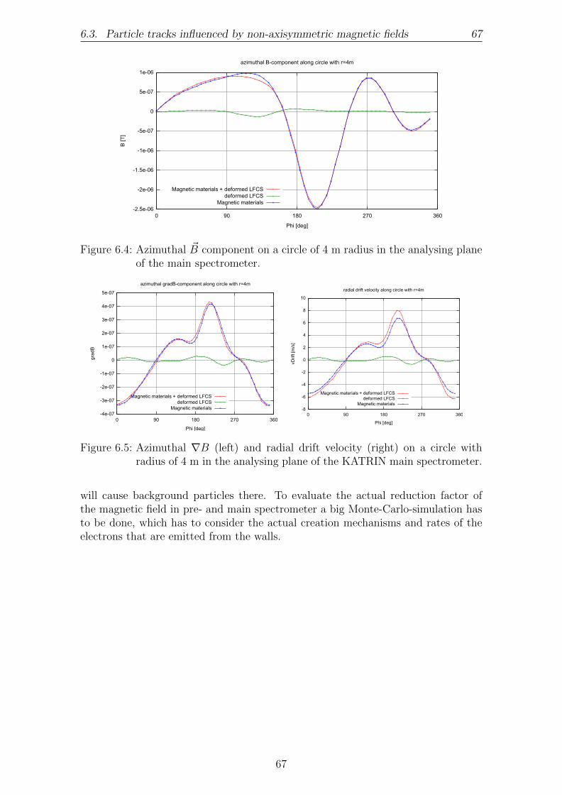
6.3. Particle tracks influenced by non-axisymmetric magnetic fields 67
-2.5e-06
-2e-06
-1.5e-06
-1e-06
-5e-07
0
5e-07
1e-06
0 90 180 270 360
B [T
]
Phi [deg]
azimuthal B-component along circle with r=4m
Magnetic materials + deformed LFCSdeformed LFCS
Magnetic materials
Figure 6.4: Azimuthal ~B component on a circle of 4 m radius in the analysing planeof the main spectrometer.
-4e-07
-3e-07
-2e-07
-1e-07
0
1e-07
2e-07
3e-07
4e-07
5e-07
0 90 180 270 360
grad
B
Phi [deg]
azimuthal gradB-component along circle with r=4m
Magnetic materials + deformed LFCSdeformed LFCS
Magnetic materials -8
-6
-4
-2
0
2
4
6
8
10
0 90 180 270 360
vDrif
t [m
/s]
Phi [deg]
radial drift velocity along circle with r=4m
Magnetic materials + deformed LFCSdeformed LFCS
Magnetic materials
Figure 6.5: Azimuthal ∇B (left) and radial drift velocity (right) on a circle withradius of 4 m in the analysing plane of the KATRIN main spectrometer.
will cause background particles there. To evaluate the actual reduction factor ofthe magnetic field in pre- and main spectrometer a big Monte-Carlo-simulation hasto be done, which has to consider the actual creation mechanisms and rates of theelectrons that are emitted from the walls.
67

68 6. Investigation of background due to non-axially-symmetric fields
Figure 6.6: Electron trajectory in the z-r plane (red). The electron started from thevessel hull with 2 eV of kinetic energy. The track was stopped in the fluxtube (blue) because a scattering event happened.
Figure 6.7: Same electron trajectory in the x-y plane (red). The black line marksthe vessel hull.
68

7. Summary and outlook
The KATRIN experiment aims to determine the mass of the electron anti-neutrinowith a sensitivity of 0.2 eV (90%C.L.). A precision measurement of the tritium-β-spectrum close to the endpoint energy will be done. The experiment uses twoMAC-E filter type spectrometers that work on the principle of magnetic adiabaticcollimation with an electrostatic filter.
This diploma work focussed on the creation and rework of new and pre-existingtools for the electromagnetic design of the KATRIN MAC-E filters. In its context,the C-codes of the magnetic and electric field calculation programmes (written byF.Gluck) were rewritten into a user friendly and flexible object oriented versionthat now forms the KAFCA (KATRIN Field CAlculation). Furthermore, a pro-grammes package that is able to simulate non axially symmetric fields and offersan interpolation method, KNAXS (partially basing on pre-existing C-routines) wasimplemented. And, together with F. Gluck, S. Mertens and N. Wandkowsky a newprogramme package to compute electron trajectories (basing on an old C-version)KTrack was implemented.
During this diploma thesis, these programmes were developed further and testedextensively. In this process, more and more compatibilities to other programme pack-ages, simulating experimental components like the source or detector, were added.So that today there exists a stable and reliable tool set for all kinds of electrontrajectory and field simulation purposes for the KATRIN experiment. And it notonly exists, its simple but sophisticated form makes it easy to use and to expand.For this reason, it established itself as standard simulation tool, used to investigateall kinds of problems in the electromagnetic design.
With the help of the KTrack, KAFCA and KNAXS packages, the study of theimpacts of non-axially symmetric magnetic field on background electrons, startingfrom the walls of the main spectrometer was started. First simulations show that,with the current stray fields in the KATRIN-hall, it is possible for low energeticelectrons (≈ 2 eV) starting from the wall to get into the flux tube, thus creating abackground signal.
69

70 7. Summary and outlook
To investigate and quantify this background, a large Monte-Carlo-Simulation withrealistic presuppositions concerning secondary electron spectra and rate has to bedone in the future. Another future task is the further integration of KTrack, KNAXSand KAFCA into the Kassiopeia framework, with the long term goal of an integrationof Kassiopeia into ORCA and ADEI, for the purposes of fast neartime simulations.
70

Bibliography
[A+96] K. Assamagan et al., “Upper limit of the muon-neutrino mass andcharged pion mass from momentum analysis of a surface muon beam,”Phys. Rev., vol. D53, pp. 6065–6077, 1996.
[A+97] W. W. M. Allison et al., “Measurement of the atmospheric neutrinoflavour composition in soudan 2,” Physics Letters B, vol. 391, p. 491,1997. [Online]. Available: doi:10.1016/S0370-2693(96)01609-7
[A+02a] J. Abdurashitov et al., “Solar neutrino flux measurements by the soviet-american gallium experiment (sage) for half the 22-year solar cycle,”Journal of Experimental and Theoretical Physics, vol. 95, no. 2, pp.181–193, 2002.
[A+02b] Q. R. Ahmad et al., “Direct evidence for neutrino flavor transformationfrom neutral-current interactions in the sudbury neutrino observatory,”Phys. Rev. Lett., vol. 89, no. 1, p. 011301, Jun 2002.
[A+03] M. Apollonio et al., “Search for neutrino oscillations on a long base-line at the CHOOZ nuclear power station,” Eur. Phys. J., vol. C27,pp. 331–374, 2003.
[A+05a] B. Aharmim et al., “A search for periodicities in the B-8 solar neutrinoflux measured by the Sudbury Neutrino Observatory,” Phys. Rev., vol.D72, p. 052010, 2005.
[A+05b] E. Aliu et al., “Evidence for muon neutrino oscillation in an accelerator-based experiment,” Phys. Rev. Lett., vol. 94, p. 081802, 2005.
[A+05c] T. Araki et al., “Measurement of neutrino oscillation with KamLAND:Evidence of spectral distortion,” Phys. Rev. Lett., vol. 94, p. 081801,2005.
[A+05d] Y. Ashie et al., “A Measurement of Atmospheric Neutrino OscillationParameters by Super-Kamiokande I,” Phys. Rev., vol. D71, p. 112005,2005.
[aaa98] T. S.-K. C. al al al al, “Study of the atmospheric neutrino fluxin the multi-gev energy range,” Physics Letters B, vol. 436, p. 33,1998. [Online]. Available: http://www.citebase.org/abstract?id=oai:arXiv.org:hep-ex/9805006
[B+82] G. Battistoni et al., “FULLY CONTAINED EVENTS IN THE MONTBLANC NUCLEON DECAY DETECTOR,” Phys. Lett., vol. B118, p.461, 1982.
71

72 Bibliography
[B+89] C. Berger et al., “Study of Atmospheric Neutrino Interactions with theFrejus Detector,” Phys. Lett., vol. B227, p. 489, 1989.
[B+98] R. Barate et al., “An upper limit on the tau neutrino mass from three-and five-prong tau decays,” Eur. Phys. J., vol. C2, pp. 395–406, 1998.
[BPG04] J. N. Bahcall and C. Pena-Garay, “Solar models and solar neutrinooscillations,” New J. Phys., vol. 6, p. 63, 2004.
[BSS] R. Beuselinck, J. Sedgbeer, and Y. Shitov. The Supernemo Exper-iment. [Online]. Available: http://www.imperial.ac.uk/research/hep/research/supernemo.htm
[Col04] K. Collaboration. (2004) KATRIN Design Report 2004. [Online].Available: http://www-ik.fzk.de/˜katrin/publications/documents/DesignReport2004-12Jan2005.pdf
[Dav94] R. Davis, “A review of the homestake solar neutrino experiment,”Progress in Particle and Nuclear Physics, vol. 32, pp. 13–32, 1994.[Online]. Available: http://www.sciencedirect.com/science/article/B6TJC-471XBFN-H/2/2af56436c91f2ca64bb2619efed29555
[DT08] N. Doss and J. Tennyson, “Excitations to the electronic continuumof 3 het + in investigations of t 2 β-decay experiments,”Journal of Physics B: Atomic, Molecular and Optical Physics,vol. 41, no. 12, p. 125701, 2008. [Online]. Available: http://stacks.iop.org/0953-4075/41/i=12/a=125701
[E+03] K. Eguchi et al., “First results from KamLAND: Evidence for reactoranti- neutrino disappearance,” Phys. Rev. Lett., vol. 90, p. 021802,2003.
[F+98] Y. Fukuda et al., “Evidence for oscillation of atmospheric neutrinos,”Phys. Rev. Lett., vol. 81, no. 8, pp. 1562–1567, Aug 1998.
[Fer34] E. Fermi, “Versuch einer Theorie der Betastrahlen,” Zeitschrift furPhysik, vol. 88, pp. 161–177, 1934.
[GGN03] M. C. Gonzalez-Garcia and Y. Nir, “Neutrino masses and mixing: evi-dence and implications,” Rev. Mod. Phys., vol. 75, no. 2, pp. 345–402,Mar 2003.
[GK07] C. Giunti and C. W. Kim, Fundamentals of Neutrino Physics andAstrophysics. Oxford Unviversity Press, 2007.
[Glu02] F. Gluck. (2002, Apr.) Runge-Kutta method for numerical solution ofdifferential equation system. [Online]. Available: http://fuzzy.fzk.de/bscw/bscw.cgi/d479152/rungekutta.pdf
[Glu06] ——. (2006) C-programs for electromagnetic design. [Online].Available: https://fuzzy.fzk.de/bscw/bscw.cgi/34401
[Glu09a] ——, “Axisymmetric electric field calculation with zonal harmonic ex-pansion,” 2009.
72
Bibliography 73
[Glu09b] ——. (2009, Mar.) Secondary electron emission in the pre-spectrometerand in the Mainz spectrometer. [Online]. Available: https://fuzzy.fzk.de/bscw/bscw.cgi/d540741/95-TRP-4652-A5-FGlueck.ppt
[GMO+09] F. Gluck, S. Mertens, A. Osipowicz, P. Plischke, J. Re-ich, and N. Wandkowsky. (2009, Mar.) Air Coil Sys-tem and Magnetic Field Sensor System. [Online]. Avail-able: http://fuzzy.fzk.de/bscw/bscw.cgi/d530439/Air%20Coil%20System%20and%20Magnetic%20Field%20Sensor%20System.pdf
[H+88] K. S. Hirata et al., “Experimental Study of the Atmospheric NeutrinoFlux,” Phys. Lett., vol. B205, p. 416, 1988.
[H+99] W. Hampel et al., “Gallex solar neutrino observations: results forgallex iv,” Physics Letters B, vol. 447, no. 1-2, pp. 127–133, 1999.[Online]. Available: http://www.sciencedirect.com/science/article/B6TVN-3VR1H2M-M/2/160790dfc1442b029b4f20ba4221d640
[Hal06] C. Hall. (2006, Oct.) Proposal for neutrino physics with supercon-ductive bolometers in DUSEL. [Online]. Available: http://mare.dfm.uninsubria.it/frontend/docs/Hall Goddard NSF Oct31.pdf
[Han05] S. Hannestad, “Neutrino mass bounds from cosmology,” NuclearPhysics B - Proceedings Supplements, vol. 145, pp. 313–318, 2005, nOW2004. [Online]. Available: http://www.sciencedirect.com/science/article/B6TVD-4G3CBPY-2C/2/a3e4c3334362d0f4e56520ea60e34197
[HK89] P. W. Hawkes and E. Kasper, Principles of Electron Optics. AcademicPress, 1989, vol. 1.
[Hot09] M. Hotzel, “Berechnung von KATRIN Messspektren unter Ein-beziehung der fensterlosen gasformigen Tritiumquelle,” Master’s thesis,Universitat Karlsruhe, 2009.
[Jac98] J. D. Jackson, “Classical electrodynamics,” 1998.
[Kay03] B. Kayser, “Neutrino Mass, Mixing, and Flavor Change,” in NeutrinoMass, G. Altarelli & K. Winter, Ed., 2003, pp. 1–+.
[KKDHK01] H. V. Klapdor-Kleingrothaus, A. Dietz, H. L. Harney, and I. V.Krivosheina, “Evidence for Neutrinoless Double Beta Decay,” Mod.Phys. Lett., vol. A16, pp. 2409–2420, 2001.
[KST87] E. W. Kolb, A. J. Stebbins, and M. S. Turner, “How reliable are neu-trino mass limits derived from sn1987a?” Phys. Rev. D, vol. 35, no. 12,pp. 3598–3606, Jun 1987.
[Las06] M. G. T. Lasserre, “Double chooz, a search for the neutrino mixingangle theta-13,” 2006. [Online]. Available: http://www.citebase.org/abstract?id=oai:arXiv.org:hep-ex/0606025
[LL02] T. J. Loredo and D. Q. Lamb, “Bayesian analysis of neutrinos observedfrom supernova sn 1987a,” Phys. Rev. D, vol. 65, no. 6, p. 063002, Feb2002.
73

74 Bibliography
[Mur08] Murayama. (2008) Oscillation Parameter Plots. [Online]. Available:http://hitoshi.berkeley.edu/neutrino/
[O+] A. Osipovicz et al. KATRIN Letter of Intend. [Online]. Available:http://www-ik1.fzk.de/tritium/publications/documents/loi.ps
[Obl] N. Oblath. Kassiopeia. [Online]. Available: http://fuzzy.fzk.de/bscw/bscw.cgi/d630345/Oblath Kassiopeia.pdf
[Pap96] L. Papula, Mathematik fur Ingenieure und Naturwissenschaftler.Vieweg + Teubner, 1996, vol. 2.
[PTVF07] W. H. Press, S. A. Teukolsky, W. T. Vetterling, and B. P. Flannery,Numerical Recipes, 3rd ed. Cambridge University Press, 2007.
[Rei10] J. Reich. (2010, Mar.) Simulation of Magnetic Materials in the MainSpectrometer Hall. [Online]. Available: http://fuzzy.fzk.de/bscw/bscw.cgi/d631077/95-TRP-4843-A3-JReich.ppt
[rep] KATRIN Software Repository. [Online]. Available: https://nustorage.uni-muenster.de/svn/katrin/
[ReW83] W. W. Repko and C. en Wu, “Radiative corrections to the end pointof the tritium β decay spectrum,” Phys. Rev. C, vol. 28, no. 6, pp.2433–2436, Dec 1983.
[ROO] ROOT, a data analysis framework. [Online]. Available: http://root.cern.ch
[Thu02] T. Thuemmler, “Entwicklung von Methoden zur Untergrun-dreduzierung am Mainzer Tritium-β-Spektrometer,” Master’s thesis,Johannes Gutenberg Universitat Mainz, Januar 2002. [Online]. Avail-able: http://fuzzy.fzk.de/bscw/bscw.cgi/d25072/dth-thuemmler1.pdf
[Ver78] J. H. Verner, “Explicit Runge-Kutta methods with estimates of thelocal truncation error,” SIAM J. Numer. Anal., vol. 15, no. 4, pp.772–790, Aug. 1978.
[Wei] C. Weinheimer, “Laboratory limits on neutrino masses,” in *Altarelli,G. (ed.) et al.: Neutrino mass* 25-52.
74

Acknowledgments
An dieser Stelle mochte ich all denjenigen Danken, die zum guten Gelingen dieserArbeit zugetragen haben. Mein Dank gebuhrt hierbei besonders folgenden Personen:
• Prof. Dr. Guido Drexlin fur die anspruchsvolle Aufgabenstellung unddie gute Betreuung wahrend der gesamten Zeit,
• Dr. Ferenc Gluck fur das Bereitstellen und Erklaren seiner zahlreichenProgramme, auf denen diese Arbeit basiert, sowie auch fur die zahlreichenphysikalischen Diskussionen, die beispielhafte Betreuung und das Korrekturlesenmeiner Arbeit,
• Dipl.-Phys. Susanne Mertens fur ihre sehr gute Betreuung, die Geduldbei technischen und physikalischen Diskussionen und bei der Beantwortung allmeiner Fragen und dem Korrekturlesen meiner Arbeit,
• Dipl.-Phys. Nancy Wandkowsky fur das eifrige Korrekturlesen dieserArbeit,
• allen Mitarbeitern des Instituts fur Kernphysik am Karlsruhe In-stitut fur Technologie fur die angenehme Arbeitsatmosphare und die stetsvorhandene Hilfsbereitschaft, sowie jedem, der nicht namentlich erwahnt ist.
Ganz besonders danken mochte ich meiner Familie, ohne deren Unterstutzung, beson-ders moralisch, aber auch finanziell, die ich wahrend meines gesamten Studiumsgenossen habe, diese Arbeit nicht moglich gewesen ware.
75