dimensionality reduction a soft set theoretic and soft

*Corresponding author

Email address: [email protected]

Songklanakarin J. Sci. Technol.

43 (4), 1063-1070, Jul. - Aug. 2021

Original Article

Dimensionality reduction - A soft set-theoretic and soft graph approach

Omdutt Sharma1, Pratiksha Tiwari2*, and Priti Gupta3

1 P. D. M. University, Bahadurgarh, Haryana, 124507 India

2 Delhi Institute of Advanced Studies, Rohini, Delhi, 110085 India

3 Maharashi Dayanand University, Rohtak, Haryana, 124507 India

Received: 29 April 2020; Revised: 25 July 2020; Accepted: 12 August 2020

Abstract

Due to the digitization of information, organizations have abundant data in databases. Large-scale data are equally

important and complex hence gathering, storing, understanding, and analyzing data is a problem for organizations. To extract

information from this superfluous data, the need for dimensionality reduction increases. Soft set theory has been efficaciously

applied and solved problems of dimensionality, which saves the cost of computation, reduces noise, and redundancy in data.

Different methods and measures are developed by researchers for the reduction of dimensions, in which some are probabilistic,

and some are non-probabilistic. In this paper, a non-probabilistic approach is developed by using soft set theory for dimensionality

reduction. Further, an algorithm of dimensionality reduction through bipartite graphs is also described. Lastly, the proposed

algorithm is applied to a case study, and a comparison of results indicates that the proposed algorithm is better than the existing

algorithms.

Keywords: dimensionality reduction, soft set, grade membership, binary-valued information system, soft graph

1. Introduction

Due to digitalization, there is a rapid growth in the

amount of information/data and the effects of this abundance

lead to difficulty in managing information, which can lead to

an overload of data that contains irrelevant and redundant data.

Handling such problems can ravage plenty of time and money.

To deal with these types of problem, there is a need to eliminate

irrelevant redundant data by a technique which is known as

dimensionality reduction. Dimensionality reduction has been a

prolific topic of study and growth, since the last four to five

decades. It has been exceptionally beneficial in eliminating

avoidable and repetitive data, increasingly effectiveness in

various areas (Gupta & Sharma, 2015). Dimension reduction

can be useful in reducing cost, redundancy, and noise. Thus, it

is one of the best tools to deal with real-life problems.

Numerous real-life situations consist of uncertainty

that cannot be successfully modeled by the classical

mathematical theories. To handle such problems contemporary

mathematical/ statistical theories were developed. Probability

theory (Kolmogorov, 1933), fuzzy sets theory (Zadeh, 1965),

rough sets theory (Pawlak, 1982), intuitionistic fuzzy sets

theory (Atansassov, 1986) and vague sets theory (Gau &

Buehre, 1993) are some of the key notions. Molodtsov (1999)

pointed out the different limitations of some of these theories.

The reason for these limitations is possibly the inadequacy of

the parameterization tool of the theories, and consequently

Molodtsov (1999) presented the notion of soft theory as a novel

mathematical tool which overcomes these limitations and

successfully applied it to the theory of games, measurement

theory, smoothness of function and Riemann integration.

Dimensionality reduction can help to solve various

decision-making problems by reducing attributes of the original

data using soft set theory. As far as the standard soft sets are

concerned, it can be defined as two different equivalence

classes of objects, thus confirming that Boolean-valued

1064 O. Sharma et al. / Songklanakarin J. Sci. Technol. 43 (4), 1063-1070, 2021

information valued systems can be dealt with by soft sets.

Maji, Roy and Biswas (2002), defined algebraic

operations for soft sets and verified binary operations for the

same. Chen, Tsang, Yeung and Wang (2005), improved the

method anticipated by Maji et al. (2002). The fuzzy soft

theoretic approach was developed to solve decision-making

problems by Roy and Maji (2007). Zhao, Luo, Wong and Yao

(2007) presented definition of reduct which jointly sufficient

and individually necessary for preserving the properties of a

given information table. Kong, Gaoa, Wang and Li (2008)

derived a heuristic normal method in soft and fuzzy soft sets for

parameter reduction. Herawan, Rose and Mat Deris (2009)

developed an approach for reduction of attributes in a multi-

valued information system in a soft theoretic environment,

which is equivalent to Pawlak’s rough reduction. Alcantud

(2016) examined relationships amongst the soft sets and other

theories. Zhan and Alcantud (2017) reviewed soft and fuzzy

soft based algorithms for parameter reduction.

Different mathematical theories focus on respective

aspects such as fuzzy, rough set and soft set theories focusing

on membership degree, granular and parameterization

respectively. Many researchers have worked on the soft set

theory which has a parameterization tool, but certain situations

involve non-Boolean datasets that require hybridization. Thus,

authors developed hybrid theories such as fuzzy soft sets

(Agman, Enginoglu, & Citak, 2011), soft rough sets (Feng et

al., 2011), fuzzy rough and rough fuzzy sets (Dubois & Prade,

1990), Soft rough fuzzy(SRF) and soft fuzzy rough (SFR) sets

(Meng et al., 2011), etc. to deal with such type of data. Zhang

and Wang (2018) investigated types of soft coverings based on

rough sets and their properties. Ma, Zhan, Ali & Mehmood

(2018) reviewed decision making methods based on hybrid

SRF and SFR sets. Zhang, Zhan and Alcantud (2019) concepts

of fuzzy soft β-minimal and β-maximal descriptions their β-

coverings and relationships amongst them. Zhang, Zhan and

Yao (2020) presented covering-based variable precision

intuitionistic fuzzy rough set models and applied multi-attribute

decision-making problems of bone transplants. Similarly, the

two papers of Jiang, Zang, Sun and Alcantud (2020) and Ma,

Zang, Sun and Alcantud (2020) worked on covering-based

variable precision fuzzy rough sets and multi-granulation fuzzy

rough set respectively and applied them to multi-attribute

decision making.

There is another non-probabilistic approach known

as graph theory, helps to model various real-life situations. This

theory is a suitable tool for solving combinatorial problems in

different areas such as geometry, algebra, number theory,

topology, operation research, optimization, and computer

science, etc. Researchers Rosenfeld (1975), Thumbakara and

George (2014), and Mohinta and Samanta (2015) combined

graph theory with the fuzzy, soft set, and fuzzy soft set theory,

respectively. Smarandache, (2018) generalized soft set to

hypersoft set by transforming the function F into a multi-

attribute function. Thereafter, introduced the hybridization of

Crisp, Fuzzy, Intuitionistic Fuzzy, Neutrosophic, and

Plithogenic Hypersoft Set. Classical techniques for reduction of

dimension are principal component analysis and multi-

dimension scaling; both are based on the concept of distance.

Graphs provide an effective way to encrypt neighborhood

relations. Burianek, Zaoralek, Snasel, and Peterek (2015)

studied select dimension reduction techniques and used them to

draw sensible graphs from initial graphs, and compared

techniques with the technique of Kamada and Kawai (1989).

Jatram and Biswas (2015) proposed a multiple dimension

reduction method of feature space of graphs by using Spectral

methods for the FANNY clustering algorithm. Qian, Yin,

Kong, Wang, and Gao (2019) presented an algorithm for low-

rank graph optimization for Multi-View Dimensionality

Reduction.

Based on the soft theoretic approach, here, a non-

probabilistic approach in dimensionality reduction is

developed. Then Boolean-valued information system is

represented as a bipartite graph and an algorithm is presented

that can be used for dimensionality reduction.

2. Related Concepts of Soft Sets and Graph Theory

A parameterized mathematical tool; soft set theory

deals with a collection of objects with categories defined

approximately. Each category has two sections - a predicate

and an estimated/ approximate value set. Since the initial

portrayal of the object has an approximate nature, the notation

of exact solution is also not required. The non-appearance of

any confinements on the approximate depictions, in soft set

theory, makes it entirely appropriate and just material

practically speaking. With the assistance of words and

sentences, real number, function, mapping, etc. any

parameterization can be utilized. Hence predicament of the

membership function or any related issue does not exist in the

soft set theory.

Definition 1 (Soft Sets): Let U represent the initial universe set

and P represent a set of parameters. Then the ordered set (m, P)

is known as soft set (on the initial universe, U) if m is a mapping

defined from P into Pow(U), where Pow(U) represents the

power set of U, i.e.

m: P → Pow(U).

Clearly, (m, P) on initial universe U represents the family of

subsets parameterized over U. Also, m(p) represents a set of p-

approximate element, for any p ϵ P for the soft set (m, P).

Example 1.1: Let U = {b1, b2, …….., b5} represents different

model of bikes and P represents different selection criteria/

parameters, P = {p1 = expensive, p2 = beautiful, p3 = cheap, p4

= in good repair, p5 = good mileage}. Then the attractiveness

of the bikes can be represented by (m, P) i.e. soft set.

Example 1.2: Let F and mF represent a fuzzy set and its

membership function respectively i.e., mF : U → [0, 1]. Let P(α)

= {x ϵ U: mF(x) greater than equal to α}, where α ϵ [0, 1]

represents family of α- level sets for mF. mF(x) can be defined

as 𝑚𝐹(𝑥) = 𝑠𝑢𝑝𝛼𝜖[0.1]

𝑥𝜖𝑃(𝛼)

𝛼, where family P is known.

Thus, every fuzzy set F can be represented as a soft set.

Alternative definition of soft sets: A pair (M, U) is defined as

a soft set over P where M is a function defined from initial

universe U to Power set of P. Alternatively in other words, a

soft set is a family of subsets of the universal parameter sets of

P. Here U is the set of objects and P is the universal set of

parameters, where parameters can be properties/

characteristics/attributes of objects.

O. Sharma et al. / Songklanakarin J. Sci. Technol. 43 (4), 1063-1070, 2021 1065

Example 1.3: Let U = {b1, b2,…….., b5} be the different sets

of cars under consideration and P be the set of parameters, P =

{p1 = price, p2 =looks, p3 = speed, p4 = weight, p5 = average}.

Then the soft set (M, U) describes the attractive cars.

2.1 Information systems equivalence with soft sets

Definition 2: Let a finite set of objects and attributes be denoted

by 𝑈 and 𝐴 respectively. Then the quadruple (𝑈, 𝐴, 𝑉, 𝑔) is

known as an information system, where 𝑔 :𝑈 × 𝐴 → 𝑉 𝑖 is

known as information function and 𝑉 = ⋃ 𝑉𝑎𝑎∈𝐴 . Also, the

value of attribute 𝑎 is given by 𝑉𝑎 = {𝑔(𝑥, 𝑎)|𝑎 ∈ 𝐴 𝑎𝑛𝑑 𝑥 ∈𝑈}.

Alternatively, An information system is known as a

knowledge representation/attribute-valued system and can be

spontaneously represented in the form of an information table

and it reduces to Boolean-valued information system if 𝑉𝑎 ={0,1}, for every 𝑎 ∈ 𝐴, in information system 𝑆 = (𝑈, 𝐴, 𝑉, 𝑔).

Proposition 1: Let (𝐹, 𝐸) be any soft set over initial universe

𝑈, then soft set (𝐹, 𝐸) can be represented as Boolean-valued

information system 𝑆 = (𝑈, 𝐴, 𝑉{0,1], 𝑔) and vice versa.

Proof: Consider (𝐹, 𝐸) and define a mapping

𝐹 = {𝑔1 , 𝑔2, … … … … . , 𝑔𝑛}.

Where

𝑔1 ∶ 𝑈 → 𝑉1 𝑎𝑛𝑑 𝑔1(𝑥) = {1, 𝑥 ∈ 𝐹(𝑒1)

0, 𝑥 ∉ 𝐹(𝑒1)

𝑔2 ∶ 𝑈 → 𝑉2 𝑎𝑛𝑑 𝑔2(𝑥) = {1, 𝑥 ∈ 𝐹(𝑒2)

0, 𝑥 ∉ 𝐹(𝑒2)

……………………………………………….

………………………………………………..

𝑔𝑛 ∶ 𝑈 → 𝑉𝑛 𝑎𝑛𝑑 𝑔𝑛(𝑥) = {1, 𝑥 ∈ 𝐹(𝑒𝑛)

0, 𝑥 ∉ 𝐹(𝑒𝑛)

Thus, for 𝐴 = 𝐸 and 𝑉 = ⋃ 𝑉𝑒𝑖𝑒𝑖∈𝐴 , for 𝑉𝑒𝑖= {0, 1}, then any

soft set (𝐹, 𝐸) can be considered as a 𝑆 = (𝑈, 𝐴, 𝑉{0,1], 𝑔) which

is a Boolean-valued information system and vice versa.

Definition 3: Let 𝑆 = (𝑈, 𝐴, 𝑉{0,1], 𝑔) be a binary-value

information system. Thus (𝐹𝑆, 𝐴) is called the soft set over 𝑈

induced by 𝑆, where 𝐹𝑆 ∶ 𝐴 → 2𝑈 and for any 𝑥 ∈ 𝑈 and 𝑎 ∈𝐴, 𝐹𝑆(𝑎) = {𝑥 ∈ 𝑈 | 𝑔(𝑥, 𝑎) = 1 𝑜𝑟 0}.

Hence, the soft set given in Example 1.1 can be

denoted as a Boolean-valued information system represented in

Table 1.

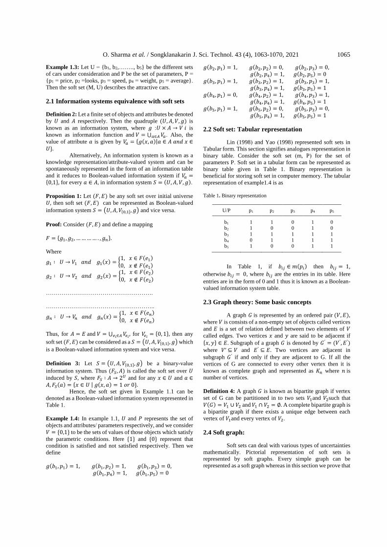
Example 1.4: In example 1.1, 𝑈 and 𝑃 represents the set of

objects and attributes/ parameters respectively, and we consider

𝑉 = {0,1} to be the sets of values of those objects which satisfy

the parametric conditions. Here {1} and {0} represent that

condition is satisfied and not satisfied respectively. Then we

define

𝑔(𝑏1, 𝑝1) = 1, 𝑔(𝑏1, 𝑝2) = 1, 𝑔(𝑏1, 𝑝3) = 0,𝑔(𝑏1, 𝑝4) = 1, 𝑔(𝑏1, 𝑝5) = 0





2.2 Soft set: Tabular representation

Lin (1998) and Yao (1998) represented soft sets in

Tabular form. This section signifies analogues representation in

binary table. Consider the soft set (m, P) for the set of

parameters P. Soft set in a tabular form can be represented as

binary table given in Table 1. Binary representation is

beneficial for storing soft set in computer memory. The tabular

representation of example1.4 is as

Table 1. Binary representation

U/P p1 p2 p3 p4 p5

b1 1 1 0 1 0 b2 1 0 0 1 0

b3 1 1 1 1 1

b4 0 1 1 1 1 b5 1 0 0 1 1

In Table 1, if 𝑏𝑖𝑗 ∈ 𝑚(𝑝𝑖) then 𝑏𝑖𝑗 = 1,

otherwise 𝑏𝑖𝑗 = 0, where 𝑏𝑖𝑗 are the entries in its table. Here

entries are in the form of 0 and 1 thus it is known as a Boolean-

valued information system table.

2.3 Graph theory: Some basic concepts

A graph 𝐺 is represented by an ordered pair (𝑉, 𝐸),

where 𝑉 is consists of a non-empty set of objects called vertices

and 𝐸 is a set of relation defined between two elements of 𝑉

called edges. Two vertices 𝑥 and 𝑦 are said to be adjacent if

{𝑥, 𝑦} ∈ 𝐸. Subgraph of a graph 𝐺 is denoted by 𝐺 ′ = (𝑉 ′, 𝐸′)

where 𝑉′ ⊆ 𝑉 and 𝐸′ ⊆ 𝐸. Two vertices are adjacent in

subgraph 𝐺 ′ if and only if they are adjacent to G. If all the

vertices of G are connected to every other vertex then it is

known as complete graph and represented as 𝐾𝑛 where 𝑛 is number of vertices.

Definition 4: A graph 𝐺 is known as bipartite graph if vertex

set of G can be partitioned in to two sets 𝑉1and 𝑉2such that

𝑉(𝐺) = 𝑉1 ∪ 𝑉2 and 𝑉1 ∩ 𝑉2 = ∅. A complete bipartite graph is

a bipartite graph if there exists a unique edge between each

vertex of 𝑉1and every vertex of 𝑉2.

2.4 Soft graph:

Soft sets can deal with various types of uncertainties

mathematically. Pictorial representation of soft sets is

represented by soft graphs. Every simple graph can be

represented as a soft graph whereas in this section we prove that


every soft set can be represented as a bipartite graph. Following

are some basic concepts:

Definition 5: A graph G represented by quadruple (𝐺∗, 𝐹, 𝐾, 𝐴)

is said to be a soft graph if following axioms are satisfied:

a) 𝐺∗(𝑉, 𝐸) represents a simple graph.

b) Set 𝐴 represents a non-empty set of parameters.

c) (𝐹, 𝐴) and (𝐾, 𝐴) both represent soft set on 𝑉 and 𝐸

respectively.

d) For all 𝑎 ∈ 𝐴,(𝐹(𝑎), 𝐾(𝑎)) represents subgraph of

𝐺∗.

The collection of all subgraphs of G is represented by 𝑆𝐺(𝐺).

Example: Consider the graph 𝐺 = (𝑉, 𝐸) as shown in Figure

1. Let 𝐴 = {1,5}. Define the set valued function 𝐹 by, 𝐹(𝑥) ={𝑦 ∈ 𝑉|𝑥 𝑅 𝑦 ⇔ 𝑑(𝑥, 𝑦) ≤ 2}.

Then 𝐹(1) = {1,2,3}, 𝐹(5) = {3,4,5}. Here 𝐹(𝑥) is a

connected subgraph of 𝐺, for all 𝑥 ∈ 𝐴. Hence (𝐹, 𝐴) ∈ 𝑆𝐺(𝐺).

Definition 5: Bipartite soft graph is defined as 𝑉(𝐺) = 𝑉1 ∪ 𝑉2

where 𝑉1 ∩ 𝑉2 = ∅, where 𝑉1 and 𝑉2 represent set of parameters

and objects respectively such that every edge of 𝐺 joins a vertex

of 𝑉1 to a vertex of 𝑉2.

Every simple graph can be represented as a soft set

and every soft set can be represented as a bipartite graph

(Hussain et al., 2016).

3. The Proposed Techniques

This section introduces a novel concept for the

reduction of parameters and objects (Dimensionality

reduction). Here the idea is to reduce dimensions of data

without changing the decision.

Definition 7: Let (m, E) represents a soft set, and 𝑚 is defined

as 𝑚 ∶ 𝐸 → 𝑃𝑜𝑤(𝑈); where 𝐸 and 𝑈 represent parameters and

universal set of objects respectively.

Let 𝐸 = {𝑒1, 𝑒2, 𝑒3, 𝑒4} and U = {𝑝1, 𝑝2, 𝑝3, 𝑝4} then

mE(𝑒1) ={𝑝1, 𝑝2, 𝑝3}, mE(𝑒2)= {𝑝3, 𝑝4}, mE(𝑒3) =

{𝑝1, 𝑝2, 𝑝3, 𝑝4}, mE(𝑒4)= {𝑝1, 𝑝3, 𝑝4}, then we define a

measure:

𝛾𝐸(𝑒𝑖) =𝑐𝑎𝑟𝑑(𝑚𝐸(𝑒𝑖))

𝑐𝑎𝑟𝑑(𝑈) Where 0 ≤ 𝛾𝐸(𝑒𝑖) ≤ 1 for all 𝑖;

where card(X) represents number of elements in set X.

Every set mE(ei) for 𝑒𝑖 ∈ 𝐸 from the parameterized

family of subsets of the set U may be considered as the set of

ei-elements of the soft set (m, E) or as the set of ei-approximate

elements of the soft sets. 𝛾𝐸(𝑒𝑖) is the grade of membership of

ei in universal set U. Here 𝛾𝐸(𝑒1) = 3/4, 𝛾𝐸(𝑒2) = 1/2, 𝛾𝐸(𝑒3) = 1 and 𝛾𝐸(𝑒4) = 3/4.

Definition 8: Let (M, U) is parameterized valued soft sets then

𝑀 ∶ 𝑈 → 𝑃𝑜𝑤(𝐸); where 𝑃𝑜𝑤(𝐸) represents power set of

universal parameterized set E and U is set of objects.

Let E = {𝑒1, 𝑒2, 𝑒3, 𝑒4} and U = {𝑝1, 𝑝2, 𝑝3, 𝑝4} then

MU(𝑝1) = {𝑒1, 𝑒3, 𝑒4} , MU(𝑝2) = {𝑒1, 𝑒3}, MU (𝑝3)=

{𝑒1, 𝑒2, 𝑒3, 𝑒4} and MU (𝑝4)= {𝑒2, 𝑒3, 𝑒4} then we define a

measure:

𝜎𝑈(𝑝𝑖) =𝑐𝑎𝑟𝑑(𝑀𝑈(𝑝𝑖))

𝑐𝑎𝑟𝑑(𝐸) ;

Figure 1. Flowchart for algorithms

where0 ≤ 𝜎𝑈(𝑝𝑖) ≤ 1 for all i; where 𝑐𝑎𝑟𝑑(𝐸) represents the

number of elements in 𝐸.

Every set MU(pi) for 𝑝𝑖 ∈ 𝑈 is the subsets of universal

parametrized set E or as the set of pi-approximate elements of

the parameterized valued soft sets. 𝜎𝑈(𝑝𝑖), is the grade of

membership of pi in the parameterized universal set E. Here

𝜎𝑈(𝑝1) = 3/4, 𝜎𝑈(𝑝2) = 1/2, 𝜎𝑈(𝑝3) = 1, 𝜎𝑈(𝑝4) = 3/4.

3.1 Algorithm for dimensionality reduction by soft set

technique

Input: The soft set (m, P)

(i) Construct table for Boolean-valued information

system with the help of soft set (m, P).

(ii) Determine 𝛾𝐸(𝑒𝑖) and 𝜎𝑈(𝑝𝑗).

(iii) Determine the cluster partition U/E according to the

value of 𝜎𝑈(𝑝𝑖).

(iv) Delete those parameters and objects for which

𝛾𝐸(𝑒𝑖) = 0 𝑎𝑛𝑑 1 and 𝜎𝑈(𝑝𝑗) = 0 respectively.

(v) Now for reduced parameters and objects go to step

(ii) and repeat the process.

(vi) If there is no reduction possible then the Boolean-

valued information system table is our desired

dimensionality reduced table.

Figure 1(i) represents flowcharts for the above-mentioned

algorithm.


Output: The dimensionality reduced the Boolean-valued

information table which gives information in decision making.

Remark: Assume that the number of objects and attributes in

the fuzzy soft set (m, P) be n and m respectively. For calculating

𝛾𝐸(𝑒𝑖) and calculating 𝜎𝑈(𝑝𝑗) comparing each entry the

complexity of computing the table is 𝑂(𝑛2).

3.2 Dimensionality reduction using soft Set

In this section example presented by Maji et al.

(2002) analyzed which was also discussed by Chen et al.

(2005). “Let U = {ℎ1, ℎ2, ℎ3, ℎ4, ℎ5, ℎ6} be a set of six houses, E

= {expensive, beautiful, wooden, cheap, in green surroundings,

modern, in good repair, in bad repair} be the set of parameters.

Let Mr. X is interested to buy a house on the subset of the

following parameter P = {beautiful, wooden, cheap, in green

surroundings, in good repair}.”

Consider the set of parameters P represented by

{𝑝1, 𝑝2, 𝑝3, 𝑝4, 𝑝5} symbolically. Boolean-valued information

system table gives the soft set as in Table 2(a). Now determine

𝛾𝑃(𝑝𝑖) and 𝜎𝑈(ℎ𝑖) using Table 2(a) given in Table 2(b). As

𝛾𝑃(𝑝1) and 𝛾𝑃(𝑝3) both are equal to 1, thus remove 𝑝1 and 𝑝3

thus Table 2(b) reduces to Table 2(c). In Table 2(c) 𝜎𝑈(ℎ5) =

0, thus remove ℎ5, now Table 2(c) reduces to Table 2(d). Again

Table 2(d), 𝛾𝑃(𝑝4) = 1, remove 𝑝4, now it reduced to Table

2(e), again 𝜎𝑈(ℎ4)=0, remove ℎ4 which reduces to Table 2(f).

Clearly, further reduction of dimensionality is not possible, so

this is the desired reduction. Here the proposed algorithm can

eliminate more parameters without changing the decision

parameter described by Maji et al. (2002). Thus, proposed

technique is better than that of Maji et al. (2002).

3.3 Reduction of parameter using bipartite graphs

Each Boolean information soft set can be

characterized by a bipartite graph. Each finite set of objects and

set of parameters represented by two vertex sets of bipartite

graph and list of adjacency contains all the 1’s. To reduce

dimensionality, the algorithm is as follows:

3.4 Algorithm for dimensionality reduction by soft set

technique

Input: The soft set (m, P)

(i) Construct table for Boolean-valued information

system by using a soft set (m, P).

(ii) Construct two bipartite graph one with having 1 as

adjacency and second with adjacency as 0. (where

one vertex set is a set of objects and the other vertex

set is a set of parameters) and name them as

membership and non- membership graphs.

(iii) Delete parameter from non- membership graph with

zero degree.

(iv) Redraw the membership graph.

(v) Delete objects with degree zero from the

membership graph.

(vi) Redraw both membership and non-membership

graphs go to step (iii) and repeat the process until no

reductions possible.

Figure 1(ii) represents flowcharts for the above-mentioned

algorithm.

Table 2. Dimensionality reduction

Table 2(a)

U/P p1 p2 p3 p4 p5 Table 2(b)

U/P p1 p2 p3 p4 p5 𝜎𝑈(ℎ𝑖)

h1 1 1 1 1 1 h1 1 1 1 1 1 1 h2 1 1 1 1 0 h6 1 1 1 1 1 1

h3 1 0 1 1 1 h2 1 1 1 1 0 4/5

h4 1 0 1 1 0 h3 1 0 1 1 1 4/5 h5 1 0 1 0 0 h4 1 0 1 1 0 3/5

h6 1 1 1 1 1 h5 1 0 1 0 0 2/5

𝛾𝑃(𝑝𝑖) 1 ½ 1 5/6 ½

Table 2(c)

U/P p1 p2 p3 p4 p5 𝜎𝑈(ℎ𝑖) Table 2(d)

U/P p1 p2 p3 p4 p5 𝜎𝑈(ℎ𝑖)

h1 1 1 1 1 h1 1 1 1 1

h6 1 1 1 1 h6 1 1 1 1

h2 1 1 0 2/3 h2 1 1 0 2/3 h3 0 1 1 2/3 h3 0 1 1 2/3

h4 0 1 0 1/3 h4 0 1 0 1/3

h5 0 0 0 0 h5 𝛾𝑃(𝑝𝑖) 1/2 5/6 ½ 𝛾𝑃(𝑝𝑖) 3/5 1 3/5

Table

2(e) U/P p1 p2 p3 p4 p5 𝜎𝑈(ℎ𝑖)

Table

2(f) U/P p1 p2 p3 p4 p5 𝜎𝑈(ℎ𝑖)

h1 1 1 1 h1 1 1 1 h6 1 1 1 h6 1 1 1

h2 1 0 ½ h2 1 0 ½

h3 0 1 ½ h3 0 1 ½ h4 0 0 0 h4

h5 h5

𝛾𝑃(𝑝𝑖) 3/5 3/5 𝛾𝑃(𝑝𝑖) 3/4 3/4


Output: Dimensionality-reduced graph which gives

information in decision making

Remark: Assume that the number of objects and

attributes in the fuzzy soft set (m, P) be n and m respectively.

For drawing both membership and non-membership graph the

complexity is 𝑂(𝑛). Since graphs are redrawn for maximum of

'm' attributes, resulting in the complexity of algorithm as

𝑂(𝑛2).

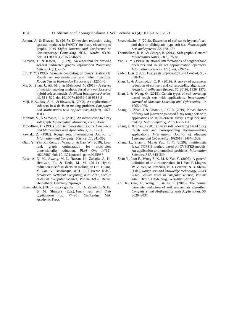
3.5 Dimensionality reduction using bipartite graph

This section discusses the example in section 3.2

using bipartite. Let U = {House 1(h1), House 2(h2), House

3(h3), House 4(h4), House 5(h5), and House 6(h6)} be a set of

six houses, Let Mr. X is interested to buy a house on the

following parameters subset P = {beautiful (P1 i.e. 7), wooden

(P2 i.e. 8), cheap (P3 i.e. 9), in green surroundings (P4 i.e. 10),

in good repair (P5 i.e. 11)}. Let {7,8,9,10,11} graphically

represents parameters.

Consider the set of parameters and objects into the

two disjoint sets of vertices of bipartite graph and edges shows

the relationship between them. By using Table 2, we draw two

types of bipartite graph as represented in Figure 2 (i)

membership graph and Figure 2(ii) non-membership graph

below:

Figure 2. (i) Membership graph (ii)Non-membership graph

Here Figure 2(i) represents sets of those objects

which satisfy the parametric conditions and Figure 2(ii)

represents sets of those objects which does not satisfy the

related parametric condition. From Figure 2 (ii) we see that

degree of 7 and 9 is zero, we remove these parameters and again

draw the bipartite graph shown in Figure 3 reduced

membership graph.

Figure 3. Reduced membership graph

From Figure 3 we see that house 5 has degree zero,

so delete house 5 and redraw membership and non-membership

bipartite graphs Figures 4(i) and 4(ii) respectively.

Figure 4. (i) Reduced membership graph (ii) Reduced non-membership graph

From reduced non-membership graph Figure 4(ii) we

see that parameter 10 has degree zero. Thus parameter 10 can

be deleted from the graph and the further reduced membership

graph is represented by Figure 5.

Figure 5. Reduced membership graph

Again, from Figure 5 it is observed that house 4 has

degree zero. Again, redraw both membership and non-

membership graph represented by Figures 6(i) and 6(ii).

Figure 6. (i) and (ii): Final reduced graph

Here Figure 6(i) represents sets of those objects

which satisfy the parametric conditions and Figure 6(ii)

represents sets of those objects which does not satisfy the

related parametric condition. In Figure 6(ii) we see that no

parameter has degree zero thus there is no parameter removal

and in Figure 6(ii) no object has zero degree thus there is no

requirement to remove any object. Thus, no further reduction is

possible.


3.6 Case study and comparative analysis

In this case study, the HOD and faculty of Statistics,

MDU University, Rohtak, India wants to add any software in

his curriculum for the students. Suggested software’s are

{SPSS, C++, R, Matlab, C-language, TORA} considering the

attributes {Job efficient (JE), Latest(L), Useful in

Statistics(US), Easy to Learn (EL), Curriculum Related (CR)}.

Based on experts views a soft-set information table is

constructed (shown in Table 3). To reduce irrelevant

information and assisting in to take the right decision, the

proposed algorithm along with some existing algorithm (Maji

et al., 2002; Rose et al., 2011) were applied to the case study.

Results based on aforesaid algorithm are given in Table 3.

According to proposed algorithm it is concluded that the HOD

and faculty of the Department may choose SPSS and R as a

curriculum. Results obtained by using the algorithm by Maji et

al. (2002) the choice values, the reduct-soft-set can be

represented in Table 3. Here max ci = c1 or c3. Thus, HOD can

choose either SPSS or R, whereas based on Rose et al. (2011)

no column presented as zero significance i.e. no parameter and

zero significance. Thus, algorithm has not eliminated or deleted

any parameter thus there is no reduction. On Comparing these

algorithms, the proposed algorithm and Maji et al. (2002) gave

same results, but the proposed algorithm eliminates parameters

as well as objects in the given information. However the Maji

et al. (2002) removes only parameters, not objects. On the other

hand, Rose et al. (2011) is not able to reduce dimension. Thus,

it can be concluded that the proposed algorithm is better than

algorithms given by both Maji et al. (2002) and Rose et al.

(2011).

4. Conclusions This paper discusses the problems of dimensionality

reduction using soft sets theory and bipartite graphs. An

alternative definition of a soft set is discussed, and new

algorithms of dimensionality reduction are presented by using

proposed techniques which are based on soft sets theory and

bipartite graphs. The proposed algorithm eliminates avoidable

parameters and objects via parameter and object importance

degree. Here we can say that our proposed technique reduces

more dimensionality and is easily applicable than the existing

ones. Hence, these algorithms execute more proficiently. The

proposed algorithm has also been applied to a case study and

obtained results were compared with algorithms by Maji et al.

(2002) and Rose et al. (2011) and found that the proposed

algorithm is more efficient than existing algorithms. But in

various real-life situations the data are not available in binary

format of 0 and 1. To overcome this problem, future scope of

work involves dimension reduction methods involving

hybridization of soft set with other theories.

References

Adams, S. M. (2002). Biological indicators of aquatic

ecosystem stress. Bethesda, MD: American Fisheries

Society.

Atanassov, K. (1986). Intuitionistic fuzzy sets. Fuzzy Sets and

Systems, 20, 87-96.

Atanassov, K. T. (1994). Operators over interval valued

intuitionistic fuzzy sets. Fuzzy sets and Systems,

64(2), 159-174.

Alcantud, J. C. R. (2016). Some formal relationships among

soft sets, fuzzy sets and their extensions.

International Journal of Approximate Reasoning, 68,

45–53.

Buriánek, T., Zaorálek, L., Snášel, V., & Peterek, T. (2015).

Graph drawing using dimension reduction methods.

In A. Abraham, P. Krömer, & V. Snasel (Eds.), Afro-

European Conference for Industrial Advancement.

Advances in Intelligent Systems and Computing,

Volume 334. Cham, Switzerland: Springer,

Chen, D., Tsang, E. C. C., Yeung, D. S., & Wang, X. (2005).

The parameterization reduction of soft sets and its

applications. Computers and Mathematics with

Applications, 49(5-6), 757-763.

Gupta, P., & Sharma, O. (2015). Feature selection: An

overview. International Journal of Information

Engineering and Technology, 1, 1- 12.

Herawan, T., Rose, A.N.M., & Mat Deris, M. (2009) Soft set

theoretic approach for dimensionality reduction. In

D. Ślęzak, T. Kim, Y. Zhang, J. Ma, & K. Chung

(Eds.), Database theory and application, DTA 2009,

Communications in computer and information

science, Volume 64. Berlin, Heidelberg, Germany:

Springer.

Hussain, Z. U., Ali, M. I., & Khan, M. Y. (2016). Application

of soft sets to determine Hamilton cycles in a graph.

General Mathematics Notes, 32. Retrieved from

www.i-csrs.orgavailablefreeonlineathttp://www.gem

an.in.

Table 3. Information table and results from different algorithms

Attributes software

Information table of Software

and attributes

Reduced

information table using

proposed

algorithm

Reduced information table using

Maji et al. (2002)

Reduced information table using

Rose et al. (2001)

JE L US EL CR JE EL JE L US EL Choice value

JE L US EL CR

SPSS 1 1 1 1 1 1 1 1 1 1 1 C1=4 - - - - - C++ 0 0 1 0 1 - - 0 0 1 0 C2=1 0 0 1 0 1

R 1 1 1 1 1 1 1 1 1 1 1 C3=4 - - - - - Matlab 1 1 1 0 1 1 0 1 1 1 0 C4=3 1 1 1 0 1

C-Language 0 0 1 0 1 - - 0 0 1 0 C5=1 0 0 1 0 1

TORA 0 1 1 1 1 0 1 0 1 1 1 C6=3 0 1 1 1 1


Jatram, A. & Biswas, B. (2015). Dimension reduction using

spectral methods in FANNY for fuzzy clustering of

graphs. 2015 Eighth International Conference on

Contemporary Computing (IC3), Noida, 93-96.

doi:10.1109/IC3.2015.7346659.

Kamada, T., & Kawai, S. (1989). An algorithm for drawing

general undirected graphs. Information Processing

Letters, 31(1), 7–15.

Lin, T. Y. (1998). Granular computing on binary relations II:

Rough set representations and belief functions.

Rough Sets in Knowledge Discovery, 1, 122-140.

Ma, X., Zhan, J., Ali, M. I. & Mehmood, N. (2018). A survey

of decision making methods based on two classes of

hybrid soft set models. Artificial Intelligence Review,

49, 511–529. doi:10.1007/s10462-016-9534-2

Maji, P. K., Roy, A. R., & Biswas, R. (2002). An application of

soft sets in a decision-making problem. Computers

and Mathematics with Applications, 44(8-9), 1077-

1083.

Mohinta, S., & Samanta, T. K. (2015). An introduction to fuzzy

soft graph. Mathematica Moravica, 19(2), 35-48.

Molodtsov, D. (1999). Soft set theory-first results. Computers

and Mathematics with Applications, 37, 19-31.

Pawlak, Z. (1982). Rough sets. International Journal of

Information and Computer Science, 11, 341-356.

Qian, Y., Yin, X., Kong, J., Wang, J., & Gao, W. (2019). Low-

rank graph optimization for multi-view

dimensionality reduction. PLoS One 14(12),

e0225987. doi: 10.1371/journal. pone.0225987

Rose, A. N. M., Awang, M. I., Hassan, H., Zakaria, A. H.,

Herawan, T., & Deris, M. M. (2011) Hybrid

reduction in soft set decision making. In D.S. Huang,

Y. Gan, V. Bevilacqua, & J. C. Figueroa (Eds.),

Advanced Intelligent Computing, ICIC 2011, Lecture

Notes in Computer Science, Volume 6838. Berlin,

Heidelberg, Germany: Springer.

Rosenfeld, A. (1975). Fuzzy graphs. In L. A. Zadeh, K. S. Fu,

& M. Shimura (Eds.), Fuzzy sets and their

applications (pp. 77–95). Cambridge, MA:

Academic Press.

Smarandache, F (2018). Extension of soft set to hypersoft set,

and then to plithogenic hypersoft set. Neutrosophic

Sets and Systems, 22, 168-170.

Thumbakara, R. K., & George, B. (2014). Soft graphs. General

Mathematics Notes, 21(2), 75-86.

Yao, Y. Y. (1998). Relational interpretations of neighborhood

operators and rough set approximation operators.

Information Sciences, 111(1-4), 239-259.

Zadeh, L. A. (1965). Fuzzy sets. Information and Control, 8(3),

338-353.

Zhan, J., & Alcantud, J. C. R. (2019). A survey of parameter

reduction of soft sets and corresponding algorithms.

Artificial Intelligence Review, 52(2019), 1839–1872.

Zhan, J. & Wang, Q. (2019). Certain types of soft coverings

based rough sets with applications. International

Journal of Machine Learning and Cybernetics, 10,

1065-1076.

Zhang, L., Zhan, J. & Alcantud, J. C. R. (2019). Novel classes

of fuzzy soft β-coverings-based fuzzy rough sets with

applications to multi-criteria fuzzy group decision

making. Soft Computing, 23, 5327–5351.

Zhang, L. & Zhan, J. (2019). Fuzzy soft β-covering based fuzzy

rough sets and corresponding decision-making

applications. International Journal of Machine

Learning and Cybernetics, 10(2019) 1487–1502.

Zhang, L., Zhan, J. M., & Yao, Y. Y. (2020). Intuitionistic

fuzzy TOPSIS method based on CVPIFRS models:

An application to biomedical problems. Information

Sciences, 517, 315-339.

Zhao Y., Luo F., Wong S. K. M. & Yao Y. (2007). A general

definition of an attribute reduct. In J. Yao, P. Lingras,

W. Z. Wu, M. Szczuka, N. J. Cercone, & D. Ślȩzak

(Eds.), Rough sets and knowledge technology, RSKT

2007, Lecture notes in computer science, Volume

4481. Berlin, Heidelberg, Germany: Springer.

Zhi, K., Gao, L., Wang, L., & Li, S. (2008). The normal

parameter reduction of soft sets and its algorithm.

Computers and Mathematics with Applications, 56,

3029–3037.

dimensionality reduction a soft set theoretic and soft

Documents