08 dimensionality redcution1
TRANSCRIPT

Dimensionality Reduction
Dr Khurram Khurshid
Pattern Recognition
Why dimensionality Reduction?
• Generally, it is easy and convenient to collect data– An experiment
• Data accumulates in an unprecedented speed• Data preprocessing is an important part for effective
machine learning• Dimensionality reduction is an effective approach to
downsizing data
2

Why dimensionality Reduction?
• Most machine learning techniques may not be effective for high-dimensional data – Curse of Dimensionality– Accuracy and efficiency may degrade rapidly as
the dimension increases.
3

Why dimensionality Reduction?
Visualization: projection of high-dimensional data onto 2D or 3D.
Data compression: efficient storage and retrieval.
Noise removal: positive effect on query accuracy.
4

Document classification
5
Internet
ACM Portal
PubMedIEEE Xplore
Digital Libraries
Web Pages Email
s
Task: To classify unlabeled documents into categories
Challenge: thousands of terms
Solution: to apply dimensionality reduction
D1
D2
Sports
T1 T2 ….…… TN
12 0 ….…… 6
DM
C
Travel
Jobs
… … …
Terms
Documents
3 10 ….…… 28
0 11 ….…… 16…
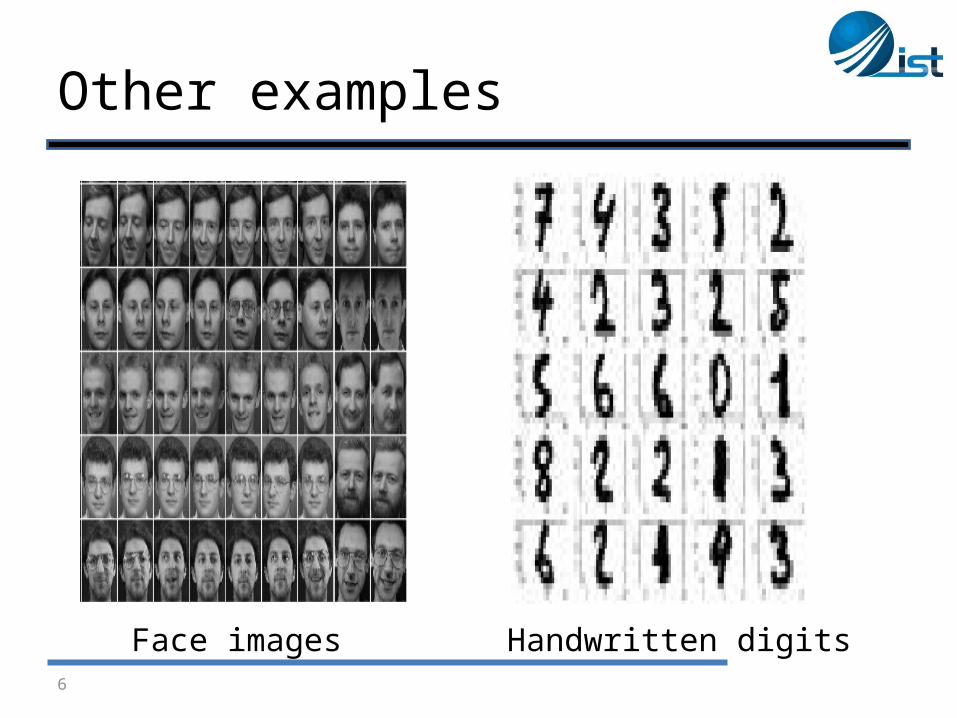
Other examples
6
Face images Handwritten digits

Dimensionality Reduction
• Reduces time complexity: Less computation
• Reduces space complexity: Less parameters
• Saves the cost of observing/computing the
feature
7

Dimensionality Reduction
8
Feature Extraction
Key methods of dimensionality reduction
Feature Selection

Feature selection vs extraction
• Feature selection:
• Feature extraction:
9
Choosing k<d important features, ignoring the remaining d – k. These are Subset selection algorithms
Project the original xi , i =1,...,d dimensions to new k<d dimensions, zj , j =1,...,k

Feature selection
10
)!mn(!m
!nm
n
Choosing an optimal subset of features (Subset of m out of n)

Feature extraction
11
)dim()dim(
)(F
xy
xy
Mapping of the original high-dimensional data onto a lower-
dimensional space

Feature extraction
Given a set of data points of p variables
Compute their low-dimensional representation:
12
nxxx ,,, 21
)( dpyx pi
di

13
Feature Selection

Contents: Feature Selection
• Introduction
• Feature subset search
• Models for Feature Selection
– Filters
– Wrappers
• Genetic Algorithm
14

Introduction
15
You have some data, and you want to use it to build a classifier, so that you can predict something (e.g. likelihood of cancer)
The data has 10,000 fields (features)

Introduction
16
You have some data, and you want to use it to build a classifier, so that you can predict something (e.g. likelihood of cancer)
The data has 10,000 fields (features)You need to cut it down to 1,000 fields beforeyou try machine learning. Which 1,000?

Introduction
17
You have some data, and you want to use it to build a classifier, so that you can predict something (e.g. likelihood of cancer)
The data has 10,000 fields (features)You need to cut it down to 1,000 fields beforeyou try machine learning. Which 1,000?
This process of choosing the 1,000 fields to use is an example of Feature Selection

Data sets with many features
18
• Gene expression datasets (~10,000 features)
• http://www.ncbi.nlm.nih.gov/sites/entrez?db=gds
• Proteomics data (~20,000 features)
• http://www.ebi.ac.uk/pride/

Feature selection: why?
19Source: http://elpub.scix.net/data/works/att/02-28.content.pdf

Feature Selection: why?
• Quite easy to find lots more cases from papers, where experiments show that accuracy reduces when you use more features
• Questions?– Why does accuracy reduce with more features?– How does it depend on the specific choice of features?– What else changes if we use more features?– So, how do we choose the right features?
20

Why accuracy reduces ?
21
Note: Suppose the best feature set has 20 features. If you add another 5 features, typically the accuracy of machine learning may reduce. But you still have the original 20 features!! Why does this happen???

Noise/explosion
• The additional features typically add noise
• Machine learning will pick up on spurious correlations, that might be true in the training set, but not in the test set
• For some ML methods, more features means more parameters to learn (more NN weights, more decision tree nodes, etc…) – the increased space of possibilities is more difficult to search
22

Feature subset search
x1
x2
X2 is important, X1 is not
x1
x2
X1 is important, X2 is not
x2
x1
x3
X1 and X2 are important, X3 is not

Subset search problem
• An example of search space (Kohavi & John 1997)
24
BackwardForward

Different aspects of search
Search starting pointsEmpty setFull set Random point
Search directionsSequential forward selectionSequential backward eliminationBidirectional generationRandom generation
Search StrategiesExhaustive/CompleteHeuristics
25

Exhaustive search
• Original dataset has N features• You want to use a subset of k features• A complete method means: try every
subset of k features, and choose the best!• The number of subsets is N! / k!(N−k)!• What is this when N is 100 and k is 5?
• What is this when N is 10,000 and k is 100?
26
75,287,520
Actually it is around 5 × 1035,101
There are around 1080 atoms in the universe

Forward Search
27
• These methods `grow’ a set S of features –
• S starts empty
• Find the best feature to add (by checking which one gives best performance on a validation set when combined with S).
• If overall performance has improved, return to step 2; else stop

Backward Search
28
• These methods ‘remove’ features one by one.
• S starts with the full feature set
• Find the best feature to remove (by checking which removal from S gives best performance on a validation set)
• If overall performance has improved, return to step 2; else stop

Models for Feature Selection
• Two models for Feature Selection– Filter methods
• Carry out feature selection independent of any learning algorithm and the features are selected as a pre-processing step
– Wrapper methods • Use the performance of a learning machine as a black
box to score feature subsets
29

Filter Methods
30
A filter method does not make use of the classifier, but rather attempts to find predictive
subsets of the features by making use of simple statistics computed from the empirical
distribution.

Filter Methods
31
CS
E D
ep
t – M
CS
-NU
ST

Filter Methods
• Ranking/Scoring of features– Select best individual features. A feature
evaluation function is used to rank individual features, then the highest ranked m features are selected.
– Although these methods can exclude irrelevant features, they often include redundant features.
– Pearson correlation coefficient
32

Filter Methods
33
maximal power in discriminating
between different classes
maximum relevance
minimal correlation among features
(members of predictor set)
minimum redundancy
a good predictor set
• Minimum Redundancy Maximum Relevance

Wrapper Methods
34
Given a classifier C and a set of feature F, a wrapper method searches in the space of
subsets of F, using cross validation to compare the performance of the trained
classifier C on each tested subset.

Wrapper Methods
35
CS
E D
ep
t – M
CS
-NU
ST

Wrapper Methods
Say we have predictors A, B, C and classifier M. We want to find the smallest possible subset of {A,B,C}, while achieving maximal performance
36
FEATURE SET CLASSIFIER PERFORMANCE
{A,B,C} M 98%
{A,B} M 98%
{A,C} M 77%
{B,C} M 56%
{A} M 89%
{B} M 90%
{C} M 91%{.} M 85%

04/15/2337
Genetic Algorithms
“Genetic Algorithms are good at taking large, potentially huge search spaces and navigating them, looking for optimal
combinations of things, solutions you might not otherwise find in a lifetime.”

First – A Biology Lesson
• A gene is a unit of heredity in a living organism• Genes are connected together into long strings called
chromosomes• A gene represents a specific trait of the organism, like
eye colour or hair colour, and has several different settings. – For example, the settings for a hair colour gene may be
blonde, black or brown etc.
• These genes and their settings are usually referred to as an organism's genotype.
• The physical expression of the genotype – the organism itself - is called the phenotype.
38

First – A Biology Lesson
• Offsprings inherit traits from parents• An offspring may end up having half the
genes from one parent and half from the other - recombination
• Very occasionally a gene may be mutated – Expressed in an organism as a completely new trait– For example: A child may have green eyes while
none of the parents had
39

Genetic Algorithm is
40
… Computer algorithm
That resides on principles of genetics and evolution
Genetic Algorithm
• Genetic algorithm (GA) introduces the principle of evolution and genetics into search among possible solutions to given problem
41
Survival of the fittestThe main principle of evolution used in GA
is “survival of the fittest”.The good solution survive, while bad ones die.

Genetic Algorithm
43

Coding
45
Genotype space = {0,1}L
Phenotype space
Encoding (representation)
Decoding(inverse representation)
011101001
010001001
10010010
10010001

Coding – Example: Feature selection
• Assume we have 15 features f1 to f15• Generate binary strings of 15 bits as initial
population
46
1 0 1 1 1 0 0 0 1 1 1 0 0 0 10 1 1 1 0 1 1 1 1 1 0 0 0 0 0………………………………………………………………1 1 1 1 0 0 0 1 1 1 0 1 1 0 1
This is initial population
Population Size= User defined parameter
1 means the feature is used – 0 means the feature is not used
One row = one chromosome =one individual of population
One gene

Fitness Function/Parent Selection
Fitness function evaluates how good an individual is in solving the problem
Fitness is computed for each individual
Fitness function is application depended
For classification – we may use the classification rate as the fitness function
Find the fitness value of each individual in the population
47

Fitness Function/Parent Selection
• Parent/Survivor Selection
– RouletteWheel Selection
– Tournament Selection
– Rank Selection
– Elitist Selection
48

Roulette Wheel Selection
• Main idea: better individuals get higher chance
• Individuals are assigned a probability of being selected based on their fitness.
pi = fi / fj
– Where pi is the probability that individual i will be selected,
– fi is the fitness of individual i, and– fj represents the sum of all the fitnesses of the
individuals with the population.
49

Roulette Wheel Selection
• Assign to each individual a part of the roulette wheel
• Spin the wheel n times to select n individuals
50
A C
1/6 = 17%
3/6 = 50%
B
2/6 = 33%
fitness(A) = 3
fitness(B) = 1
fitness(C) = 2

Roulette Wheel Selection
51

Roulette Wheel Selection
52
No. String Fitness % Of Total
1 01101 169 14.4
2 11000 576 49.2
3 01000 64 5.5
4 10011 361 30.9
Total 1170 100.0

Roulette Wheel Selection
53
Chromosome1
Chromosome 2
Chromosome 3
Chromosome 4

Tournament Selection
• Binary tournament– Two individuals are randomly chosen; the fitter
of the two is selected as a parent
• Larger tournaments– n individuals are randomly chosen; the fittest
one is selected as a parent
54

Other Methods
• Rank Selection– Each individual in the population is assigned a
numerical rank based on fitness, and selection is based on this ranking.
• Elitism– Reserve k slots in the next generation for the
highest scoring/fittest chormosomes of the current generation
55

Reproduction
• Reproduction operators– Crossover– Mutation
• Crossover is usually the primary operator with mutation serving only as a mechanism to introduce diversity in the population
56
Reproduction
• Crossover– Two parents produce two offspring– There is a chance that the chromosomes of the two parents are
copied unmodified as offspring– There is a chance that the chromosomes of the two parents are
randomly recombined (crossover) to form offspring– Generally the chance of crossover is between 0.6 and 1.0
• Mutation– There is a chance that a gene of a child is changed randomly– Generally the chance of mutation is low (e.g. 0.001)
57

Crossover
• Generating offspring from two selected parents– Single point crossover– Two point crossover (Multi point crossover)– Uniform crossover
58

One pont crossover
• Choose a random point on the two parents• Split parents at this crossover point• Create children by exchanging tails
59

One pont crossover
• Choose a random point on the two parents• Split parents at this crossover point• Create children by exchanging tails
60
Parent 1: X X | X X X X XParent 2: Y Y | Y Y Y Y YOffspring 1: X X Y Y Y Y YOffspring 2: Y Y X X X X X

Crossover
61
11101100000001
00101111001000
00110010001100
00101111000110
Crossover point

Crossover
62
1110111100011011101100000001
00101111001000
00110010001100
0010110000000100101111000110

Crossover
63
1110111100011011101100000001
0010101000110000101111001000
0011011100100000110010001100
0010110000000100101111000110

Two point corssover
• Two-Point crossover is very similar to single-point crossover except that two cut-points are generated instead of one.
64
Parent 1: X X | X X X | X XParent 2: Y Y | Y Y Y | Y YOffspring 1: X X Y Y Y X XOffspring 2: Y Y X X X Y Y

N point crossover
• Choose n random crossover points• Split along those points• Glue parts, alternating between parents
65

Uniform corssover
A random mask is generatedThe mask determines which bits are copied from
one parent and which from the other parentBit density in mask determines how much material
is taken from the other parent
66
Mask: 0110011000 (Randomly generated)Parents: 1010001110 0011010010
Offspring: 0011001010 1010010110
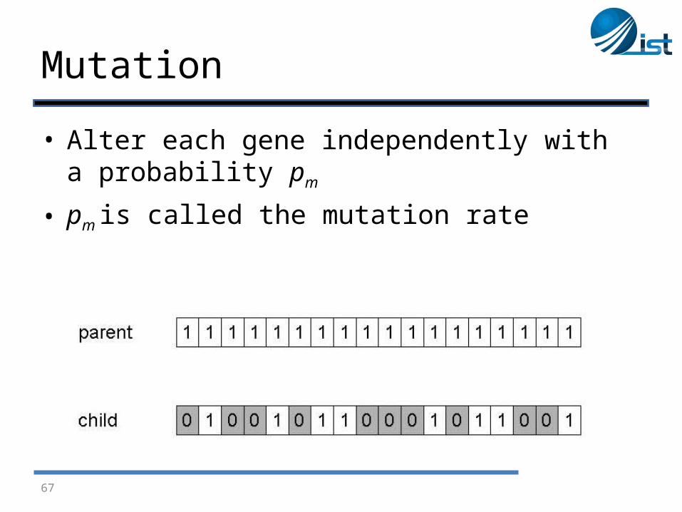
Mutation
• Alter each gene independently with a probability pm
• pm is called the mutation rate
67

Summary – Reproduction cycle
• Select parents for producing the next generation
• For each consecutive pair apply crossover with probability pc , otherwise copy parents
• For each offspring apply mutation (bit-flip with probability pm)
• Replace the population with the resulting population of offsprings
68

Convergence
• Stop Criterion– Number of generations– Fitness value
• How fit is the fittest individual
69

GA for feature selection
• The initial population is randomly generated• Each chromosome is evaluated using the
fitness function• The fitness values of the current population
are used to find the off springs of the next generation
• The generational process ends when the termination criterion is satisfied
• The selected features correspond to the best individual in the last generation
70

GA for feature selection
• GA can be executed multiple times• Example: 15 features, GA executed 10 times
71
0 1 2 3 4 5 6 7 8 9 10
f1
f2
f3
f4
f5
f6
f7
f8
f9
f10
f11
f12
f13
f14
f15
Fe
atu
re
Number of times selected

GA for feature selection
• Feature categories based on frequency of selection
• Indispensable:– Feature selected in each selected feature
subset.
• Irrelevant:– Feature not selected in any of the selected
subsets.
• Partially Relevant: – Feature selected in some of the subsets.
72

GA Worked Example
Suppose that we have a rotary system (which could be mechanical - like an internal combustion engine or gas turbine, or electrical - like an induction motor).
The system has five parameters associated with it - a, b, c, d and e. These parameters can take any integer value between 0 and 10.
When we adjust these parameters, the system responds by speeding up or slowing down.
Our aim is to obtain the highest speed possible in revolutions per minute from the system.
73

GA Worked Example
• Generate a population of random strings (we’ll use ten as an example):
74
Step 1

GA Worked Example
Feed each of these strings into the machine, in turn, and measure the speed in revolutions per minute of the machine. This value is the fitness because the higher the speed, the better the machine:
75
Step 2

GA Worked Example
• To select the breeding population, we’ll go the easy route and sort the strings then delete the worst ones. First sorting:
76
Step 3

GA Worked Example
• Having sorted the strings into order we delete the worst half
77
Step 3

GA Worked Example
• We can now crossover the strings by pairing them up randomly. Since there’s an odd number, we’ll use the best string twice. The pairs are shown below:
78
Step 4

GA Worked Example
• The crossover points are selected randomly and are shown by the vertical lines. After crossover the strings look like this:
79
These can now join their parents in the next generation
Step 4

GA Worked Example
• New Generation
80
Step 4

GA Worked Example
• We have one extra string (which we picked up by using an odd number of strings in the mating pool) that we can delete after fitness testing.
81
Step 4

GA Worked Example
• Finally, we have mutation, in which a small number of numbers are changed
82
Step 5

GA Worked Example
• After this, we repeat the algorithm from stage 2, with this new population as the starting point.
• Keep repeating until convergence
83
GA Worked Example
• Roulette Wheel Selection– The alternative (roulette) method of selection
would make up a breeding population by giving each of the old strings a chance of ending up in the breeding population which is proportional to its fitness
– Making the fitness for each string the addition of its own fitness with all of those before it
84

GA Worked Example
• Roulette Wheel Selection
85
1. If we now generate a random number between 0 and 10280 we can use this to select strings.
2. If the random number turns out to be between 0 and 100 then we choose the last string.
3. If it’s between 8080 and 10280 we choose the first string. 4. If it’s between 2480 and 3480 we choose the string 3 6 8
6 9, etc. You don’t have to sort the strings into order to use this method.

86
Feature Extraction

Feature Extraction
• Unsupervised– Principal Component Analysis (PCA)– Independent Component Analysis (ICA)
• Supervised– Linear Discriminant Analysis (LDA)
87

Principal component Analysis (PCA)• PCA is one of the most common feature
extraction techniques• Reduce the dimensionality of a data set by
finding a new set of variables, smaller than the original set of variables
• Allows us to combine much of the information contained in n features into m features where m < n
88

PCA – Introduction
89
2z
1z
• The 1st PC is a minimum distance fit to a line in X space• The 2nd PC is a minimum distance fit to a line in the plane perpendicular to the 1st PC
PCs are a series of linear least squares fits to a sample,each orthogonal to all the previous.
1z

Principal component Analysis (PCA)
90

PCA – Introduction
Transform n-dimensional data to a new n-dimensions
The new dimension with the most variance is the first principal component
The next is the second principal component, etc.
91

Variance and Covariance
• Variance is a measure of data spread in one dimension (feature)
• Covariance measures how two dimensions (features) vary with respect to each other
92
Recap

Covariance
• Focus on the sign (rather than exact value) of covariance– Positive value means that as one feature
increases or decreases the other does also (positively correlated)
– Negative value means that as one feature increases the other decreases and vice versa (negatively correlated)
– A value close to zero means the features are independent
93
Recap

Covariance Matrix
• Covariance matrix is an n × n matrix containing the covariance values for all pairs of features in a data set with n features (dimensions)
• The diagonal contains the covariance of a feature with itself which is the variance (which is the square of the standard deviation)
• The matrix is symmetric
94
Recap

PCA – Main Steps
95
Center data around 0
Form the covariance matrix S.
Compute its eigenvectors:
The first p eigenvectors form the p PCs.
The transformation G consists of the p PCs.
],,,[ 21 paaaG
d
iia 1
p
iia 1
A test point d T px G x

PCA – Worked Example
96
2.5 2.4
0.5 0.7
2.2 2.9
1.9 2.2
3.1 3.0
2.3 2.7
2.0 1.6
1.0 1.1
1.5 1.6
1.2 0.9
X Y
Data

PCA – Worked Example
97
Step 1
First step is to center the original data around 0 Subtract mean from each value
X Y
2.5 2.4
0.5 0.7
2.2 2.9
1.9 2.2
3.1 3.0
2.3 2.7
2.0 1.6
1.0 1.1
1.5 1.6
1.2 0.9
X 1.81
Y 1.91
X Y
0.69 0.49
1.31 1.21
0.39 0.99
0.09 0.29
1.29 1.09
0.49 0.79
0.19 0.31
0.81 0.81
0.31 0.31
0.71 1.01

PCA – Worked Example
• Calculate the covariance matrix of the centered data – Only 2 × 2 for this case
98
Step 2
X Y
2.5 2.4
0.5 0.7
2.2 2.9
1.9 2.2
3.1 3.0
2.3 2.7
2.0 1.6
1.0 1.1
1.5 1.6
1.2 0.9
X 1.81
Y 1.91
X Y
0.69 0.49
1.31 1.21
0.39 0.99
0.09 0.29
1.29 1.09
0.49 0.79
0.19 0.31
0.81 0.81
0.31 0.31
0.71 1.01
cov 0.616555556 0.615444444
0.615444444 0.716555556
cov(X,Y ) X i X Yi Y
i1
n
n 1

PCA – Worked Example
• Calculate the eigenvectors and eigenvalues of the covariance matrix (remember linear algebra)– Covariance matrix – square n × n ; n eigenvalues will exist
– All eigenvectors (principal components/dimensions) are orthogonal to each other and will make a new set of dimensions for the data
– The magnitude of each eigenvalue corresponds to the variance along that new dimension – Just what we wanted!
– We can sort the principal components according to their eigenvalues
– Just keep those dimensions with largest eigenvalues
99
Step 3
eigenvalues0.490833989
1.28402771
eigenvectors 0.735178656 0.677873399
0.677873399 0.735178656

PCA – WORKED EXAMPLE
100
Step 3
Two eigenvectors overlaying the centered data

PCA – WORKED EXAMPLE
• Just keep the p eigenvectors with the largest eigenvalues– Do lose some information, but if we just drop
dimensions with small eigenvalues then we lose only a little information
– We can then have p input features rather than n– How many dimensions p should we keep?
101 1 2 3 4 5 6 7 … n
Eigenvalue
i
i1
p
i
i1
n
1 2 p
1 2 p n
Proportionof Variance
Step 4

PCA – WORKED EXAMPLE
• Proportion of Variance (PoV)
when λi are sorted in descending order
• Typically, stop at PoV>0.9
102
1 2
1 2
p
p n
Step 4

PCA – WORKED EXAMPLE
103
Step 4

PCA – WORKED EXAMPLE
• Transform the features to the p chosen Eigenvectors• Take the p eigenvectors that you want to keep from the list
of eigenvectors, and forming a matrix with these eigenvectors in the columns.
• For our example; either keep both vectors or chose to leave out the smaller less significant one
104
0.677873399 0.735178656
0.735178656 0.677873399
0.677873399
0.735178656
OR
1 2( .... )pFeature vector eig eig eig
Step 4

PCA – WORKED EXAMPLE
• RowFeatureVector is matrix with eigenvectors in the columns transposed so that eigenvectors are now in the rows with most significant eigenvector at the top
• RowDataAdjust is the mean-adjusted data transposed
• FinalData is the final data set with data items in columns and dimensions along the rows
105
FinalData = RowFeatureVector x RowDataAdjust
Step 5

PCA – WORKED EXAMPLE
106
Step 5
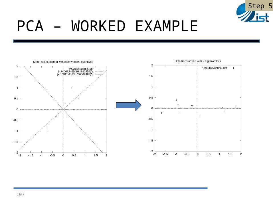
PCA – WORKED EXAMPLE
107
Step 5

PCA – WORKED EXAMPLE
108
Step 5

PCA – WORKED EXAMPLE
• Getting back original data– We used the transofrmation
– This gives
– In our case, inverse of feature vector is equal to its transpose
109
FinalData = RowFeatureVector x RowDataAdjust
RowDataAdjust = RowFeatureVector-1 x FinalData
RowDataAdjust = RowFeatureVectorT x FinalData

PCA – WORKED EXAMPLE
• Getting back original data– Add mean to get back raw data:
• If we use all (two in our case) eigenvectors we get back exactly the original data
• With one eigenvector, some information is lost
110
OriginalData= (RowFeatureVectorT x FinalData) + Mean

PCA – WORKED EXAMPLE
111
Original Data Original Data restored with one eigenvector

PCA Applications
• Eigenfaces for recognition. Turk and Pentland. 1991.
• Principal Component Analysis for clustering gene expression data. Yeung and Ruzzo. 2001.
• Probabilistic Disease Classification of Expression-Dependent Proteomic Data from Mass Spectrometry of Human Serum. Lilien. 2003.
112