dimensionality-reduced estimation of primaries by · pdf fileazimuth seismic recording and...

Dimensionality-reduced estimation of primaries by

sparse inversion

Bander Jumah and Felix J. HerrmannDepartment of Earth and Ocean sciences, University of British Columbia,

Vancouver, Canada

ABSTRACT

Data-driven methods—such as the estimation of primaries by sparse inversion—suffer from the ’curse of dimensionality’ that leads to disproportional growthin computational and storage demands when moving to realistic 3D field data.To remove this fundamental impediment, we propose a dimensionality-reductiontechnique where the ’data matrix’ is approximated adaptively by a randomizedlow-rank factorization. Compared to conventional methods, which need for eachiteration passage through all data possibly requiring on-the-fly interpolation, ourrandomized approach has the advantage that the total number of passes is re-duced to only one to three. In addition, the low-rank matrix factorization leadsto considerable reductions in storage and computational costs of the matrix mul-tiplies required by the sparse inversion. Application of the proposed method tosynthetic and real data shows that significant performance improvements in speedand memory use are achievable at a low computational up-fron cost required bythe low-rank factorization.

INTRODUCTION

Demand for oil and gas is increasing rapidly while new discoveries are more difficultto make because most of the relatively easy to find reservoirs are being depleted.This development combined with high oil prices and the decline of conventional oilreserves are the driving forces behind continued efforts of the oil and gas industrytowards unconventional and more difficult to find and produce reservoirs. In orderto achieve this ambition, state-of-the-art technologies, such as high-density, wide-azimuth seismic recording and imaging, are now being utilized to generate higherresolution images of the earth’s subsurface.

Unfortunately, these new technologies generate enormous volumes of 3D data thatrequire massive amounts of computational resources to store, manage, and processes.For example, it is nowadays not unusual to conduct seismic surveys that gather onemillion traces per square mile, which is a significant increase compared the 10,000traces that were collected traditionally for this area. This development not onlymakes the acquisition costly but it also makes processing these massive data volumes

The University of British Columbia Technical Report. TR-2012-01, February 15, 2012

Jumah and Herrmann 2 dimensionality-reduced EPSI

extremely challenging. These challenges become particularly apparent in the caseof data-driven seismic methods, e.g. Surface-Related Multiple Elimination (SRME,Berkhout and Verschuur, 1997) and Estimation of Primaries by Sparse Inversion(EPSI, van Groenestijn and Verschuur, 2009; Lin and Herrmann, 2011, 2012). Thesemethods are known to be compute intensive because they rely on multi-dimensionalconvolutions that translate into massive dense matrix-vector multiplies, and therefore,suffer from the “curse of dimensionality”, where the size of the data volume increasesexponentially with the and survey area and desired resolution. For example, in 3D adata set with of 1000 sources and receivers results in multiplications for each frequencyof dense matrices of size 10006 × 10006. Needless to say these matrices can not bestored, are expensive to apply, and often require on-the-fly interpolation becauseacquired data is nearly always incomplete.

Working with massive data volumes also creates communication bottlenecks thatform a major impediment for iterative methods that require multiple passes throughall data. For this reason, current-day seismic data processing centers spend approxi-mately the same amount of time on running SRME as on migration and this explainsthe slow adaption of EPSI by industry this technique requires more passes throughthe data.

We present a dimensionality-reduction technique that is aimed at limiting thenumber of passes over the data (including on-the-fly-interpolation) to one to threewhile reducing the memory imprint, accelerating the matrix multiplications, andleveraging parallel capabilities of modern computer architectures. A low-rank ma-trix factorization with the randomized singular-value decomposition (SVD, Halkoet al., 2011) lies at the heart of our method. We use this factorization to approximatethe action of monochromatic ’data matrices’, whose columns are given by seismicshot records. For early application of SVDs to data matrices, we refer to Minatoet al. (2011). By selecting the rank of each monochromatic data matrix adaptively,we are able to approximate matrix multiplies with a controllable error. Because therandomized SVD only requires the action of the data matrix on some set of randomvectors, our algorithm can work with existing code bases for SRME.

A key step in the randomized SVD is formed by matrix probing (Halko et al.,2011; Chiu and Demanet, 2012; Demanet et al., 2012), where information on therange of a matrix is obtained by applying the matrix on a small set of random testvectors. The number of these vectors depends on the rank of the matrix, which in turndetermines the degree of dimensional reduction and speedup yielded by the low-rankapproximation. While standard SVDs are of limited value to large-scale problems,the proposed randomized SVD is well suited to computer architectures that can dofast matrix multiplies but that have difficulties moving large amounts of data in andout of memory.

The paper is organized as follows. First, we briefly introduce EPSI by recastingBerkhout’s data matrix into a vectorized form, which makes it conducive to curvelet-domain sparsity promotion. Next, we identify that the matrix multiplies are thedominant cost and we show that these costs can be reduced by replacing the data



matrix for each frequency by a low-rank factorization with SVDs. To get betteraccuracy, we propose an adaptive scheme that selects the appropriate ranks for eachdata matrix depending on their spectral norm. Next, we introduce the randomizedSVD based on matrix probing. This technique allows us to carry out the SVD on largesystems. Because data often has missing shots, we also discuss how matrix probingcan be extended so that it no longer relies on full sampling or on-the-fly interpolationbut instead can work with data with missing shots directly. We show for either casethat matrix probing leads to a significant reduction in the number passes through datanot only for the calculation of the factorizations but also for the iterative solutionof EPSI. To address the increase in rank with frequency, we introduce HierarchicallySemi-Separable Matrix Representation (HSS, Lin et al., 2011) matrices. Finally, weconclude by performing tests of our method on synthetic and real seismic lines.

THEORY

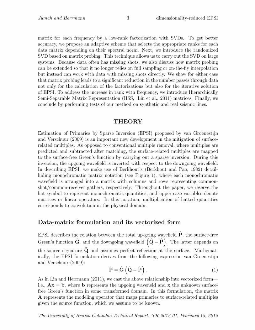
Estimation of Primaries by Sparse Inversion (EPSI) proposed by van Groenestijnand Verschuur (2009) is an important new development in the mitigation of surface-related multiples. As opposed to conventional multiple removal, where multiples arepredicted and subtracted after matching, the surface-related multiples are mappedto the surface-free Green’s function by carrying out a sparse inversion. During thisinversion, the upgoing wavefield is inverted with respect to the downgoing wavefield.In describing EPSI, we make use of Berkhout’s (Berkhout and Pao, 1982) detail-hiding monochromatic matrix notation (see Figure 1), where each monochromaticwavefield is arranged into a matrix with columns and rows representing common-shot/common-receiver gathers, respectively. Throughout the paper, we reserve thehat symbol to represent monochromatic quantities, and upper-case variables denotematrices or linear operators. In this notation, multiplication of hatted quantitiescorresponds to convolution in the physical domain.

Data-matrix formulation and its vectorized form

EPSI describes the relation between the total up-going wavefield P, the surface-free

Green’s function G, and the downgoing wavefield(Q− P

). The latter depends on

the source signature Q and assumes perfect reflection at the surface. Mathemat-ically, the EPSI formulation derives from the following expression van Groenestijnand Verschuur (2009):

P = G(Q− P

). (1)

As in Lin and Herrmann (2011), we cast the above relationship into vectorized form—i.e., Ax = b, where b represents the upgoing wavefield and x the unknown surface-free Green’s function in some transformed domain. In this formulation, the matrixA represents the modeling operator that maps primaries to surface-related multiplesgiven the source function, which we assume to be known.



To arrive at this formulation, which includes Fourier and sparsiying transforms, weuse the relation vec (AXB) =

(BT ⊗A

)vec (X), which holds for arbitrary matrices

– of compatible sizes – A,X, and B. In this expression, the symbol ⊗ refers to theKronecker product and vec stacks the columns of a matrix into a long concatenatedvector (matlab’s colon operator). Equation 1, can now be rewritten as(

(Q− P)Ti ⊗ I)

vec(Gi

)= vec

(Pi

), i = 1 · · ·nf , (2)

where I is the identity matrix. After inclusion of the temporal Fourier transform(Ft = (I ⊗ I ⊗Ft) with Ft the temporal Fourier transform), we arrive at the followingblock-diagonal system:

F∗t

(

(Q− P)T1 ⊗ I)

. . . ((Q− P)Tnf

⊗ I)Ft

︸︷︷︸U

vec (G1)...

vec (Gnt)

︸︷︷︸

g

=

vec (P1)...

vec (Pnt)

︸︷︷︸

p

. (3)

In this expression, we use the symbol ∗ to denote the Hermitian transpose or adjoint.

The above vectorized equation is amenable to transform-domain sparsity promo-tion by defining A := US∗, where g = S∗x is the transform-domain representation ofg and S the sparsifying transform. We use a combination of the 2D curvelet, along thesource-receiver coordinates, and the 1D wavelet transform along the time coordinates.Using the Kronecker product again, we define S = C ⊗W. With these definitions,we relate the sparsifying representation for the surface-free Green’s function to thevectorized upgoing wavefield b = vec (P) via Ax = b. This relationship forms thebasis for our inversion.

Sparse inversion

Solving for the transform-domain representation of the surface-free Green’s functiong(t, xs, xr) with t time, xs the source and xr the receiver coordinates, correspondsafter discretization to inverting a linear system of equations where the monochro-matic wavefields {(Q − P)i}i=1···nf

and temporal wavefields {Pi}i=1···nt are related—through the temporal Fourier transform—to the curvelet-wavelet representation ofthe discretized wavefield vector g in the physical domain (cf. Equation 3). To controlissues related to the null-space of A, we solve this system by promoting sparsity—i.e,we solve

x = arg minx‖x‖1 subject to ||Ax− b||2 ≤ σ, (4)

where σ is the error between the predicted and recorded data.

Solving these optimization problems requires multiple iterations. Each of theseiterations are challenging for real applications in 3D because (i) the matrices are



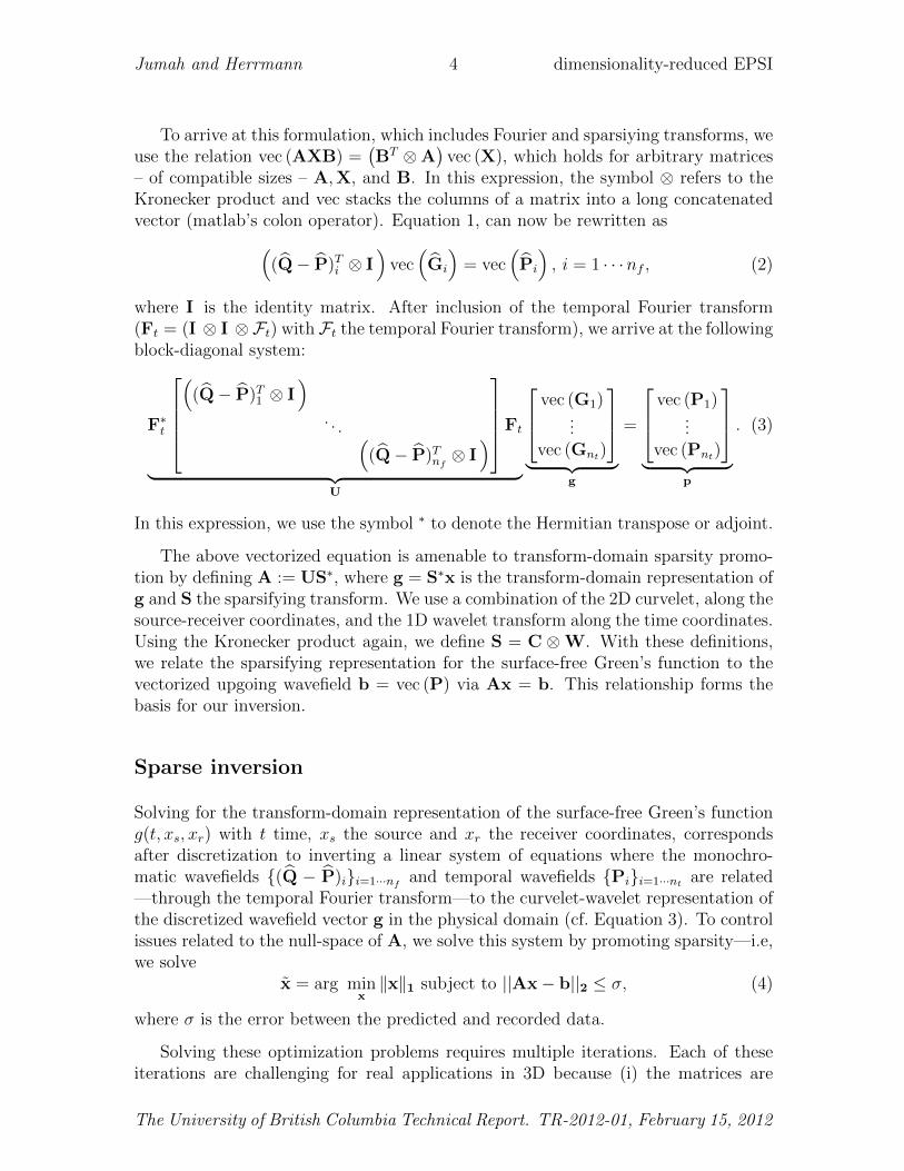
dense and extremely large, e.g. for each frequency the data matrix becomes easily106 × 106 for ns = nr = 1000 (with ns the number of sources and nr the number ofreceivers). This means that these optimizations require lots of storage and computa-tional resources to carry-out the multiplications; (ii) The collected data volumes areincomplete, which makes it necessary to carry out ’on-the-fly’ interpolations that arecostly but that have the advantage that the data matrix does not need to be storedand formed explicitly; and (iii) the solvers require multiple evaluations of A, A∗, andpossibly A∗A. Remember, each of these matrix-vector operations include a Fourier,curvelet, and wavelet transforms, and the application of the data matrix. While thetransforms can be carried out relatively quickly, the application of the data matrix re-quires a complete pass over all data during which data needs to be transferred in andout of main memory. In practice, this leads to processing times that are of the sameorder of migration for a single iteration. To reduce these storage and multiplicationcosts, we replace the data matrix by a low-rank approximation using Singular-ValueDecomposition (SVD).

Figure 1: Extraction of monochromatic wavefield matrices, by transforming the datafrom the time domain into the frequency domain via the Fourier transform. Then,for each frequency component a data matrix P ∈ Cnr×ns is extracted (adapted fromDedem (2002)).

Dimensionality reduction via singular-value decomposition

To limit the storage and multiplication costs, we approximately factorize the datamatrix into

Pnr×ns ≈ Lnr×kR∗k×ns

, (5)

where the symbol ≈ refers to an approximation with a controllable error. In thisformulation, a data matrix with nr receivers and ns sources is factorized into muchsmaller tall and fat matrices that reduce the computational and memory costs of



applying the data matrix. The approximation is low rank if the error is small fork << min(nr, ns).

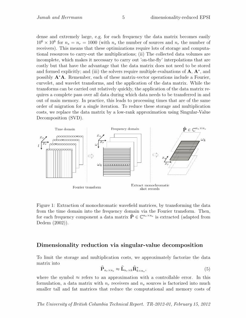
A special case of a low-rank matrix factorization is the Singular Value Decompo-sition (SVD) where the data matrix P is decomposed into three factors, namely

Pnr×ns ≈ Unr×kSk×kV∗k×ns

, (6)

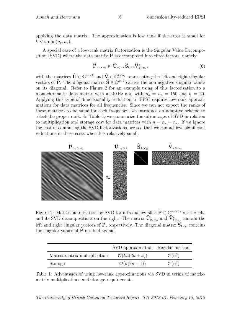
with the matrices U ∈ Cnr×k and V ∈ Ck×ns representing the left and right singularvectors of P. The diagonal matrix S ∈ Ck×k carries the non-negative singular valueson its diagonal. Refer to Figure 2 for an example using of this factorization to amonochromatic data matrix with at 40 Hz and with ns = nr = 150 and k = 20.Applying this type of dimensionality reduction to EPSI requires low-rank approxi-mations for data matrices for all frequencies. Since we can not expect the ranks ofthese matrices to be same for each frequency, we introduce an adaptive scheme toselect the proper rank. In Table 1, we summarize the advantages of SVD in relationto multiplication and storage cost for data matrices with n = ns = nr. If we ignorethe cost of computing the SVD factorizations, we see that we can achieve significantreductions in these costs when k is relatively small.

Figure 2: Matrix factorization by SVD for a frequency slice P ∈ Cnr×ns on the left,and its SVD decompositions on the right. The matrix Unr×k and V∗k×ns

contain the

left and right singular vectors of P, respectively. The diagonal matrix Sk×k containsthe singular values of P on its diagonal.

SVD approximation Regular method

Matrix-matrix multiplication O(kn(2n+ k)) O(n3)

Storage O(k(2n+ 1)) O(n2)

Table 1: Advantages of using low-rank approximations via SVD in terms of matrix-matrix multiplications and storage requirements.



Adaptive low-rank approximation

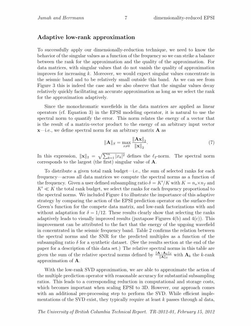
To successfully apply our dimensionally-reduction technique, we need to know thebehavior of the singular values as a function of the frequency so we can strike a balancebetween the rank for the approximation and the quality of the approximation. Fordata matrices, with singular values that do not vanish the quality of approximationimproves for increasing k. Moreover, we would expect singular values concentrate inthe seismic band and to be relatively small outside this band. As we can see fromFigure 3 this is indeed the case and we also observe that the singular values decayrelatively quickly facilitating an accurate approximation as long as we select the rankfor the approximation adaptively.

Since the monochromatic wavefields in the data matrices are applied as linearoperators (cf. Equation 3) in the EPSI modeling operator, it is natural to use thespectral norm to quantify the error. This norm relates the energy of a vector thatis the result of a matrix-vector product to the energy of an arbitrary input vectorx—i.e., we define spectral norm for an arbitrary matrix A as

‖A‖S = maxx 6=0

‖Ax‖2‖x‖2

. (7)

In this expression, ‖x‖2 =√∑n

k=1 |xk|2 defines the `2-norm. The spectral normcorresponds to the largest (the first) singular value of A.

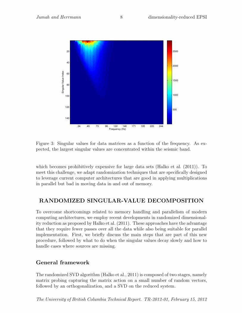
To distribute a given total rank budget—i.e., the sum of selected ranks for eachfrequency—across all data matrices we compute the spectral norms as a function ofthe frequency. Given a user defined subsampling ratio δ = K ′/K withK = ns×nf andK ′ � K the total rank budget, we select the ranks for each frequency proportional tothe spectral norms. We included Figure 4 to illustrate the importance of this adaptivestrategy by comparing the action of the EPSI prediction operator on the surface-freeGreen’s function for the compete data matrix, and low-rank factorizations with andwithout adaptation for δ = 1/12. These results clearly show that selecting the ranksadaptively leads to visually improved results (juxtapose Figures 4(b) and 4(c)). Thisimprovement can be attributed to the fact that the energy of the upgoing wavefieldin concentrated in the seismic frequency band. Table 2 confirms the relation betweenthe spectral norms and the SNR for the predicted multiples as a function of thesubsampling ratio δ for a synthetic dataset. (See the results section at the end of thepaper for a description of this data set.) The relative spectral norms in this table are

given the sum of the relative spectral norms defined by ‖A−Ak‖S‖A‖S

with Ak the k-rankapproximation of A.

With the low-rank SVD approximation, we are able to approximate the action ofthe multiple prediction operator with reasonable accuracy for substantial subsamplingratios. This leads to a corresponding reduction in computational and storage costs,which becomes important when scaling EPSI to 3D. However, our approach comeswith an additional pre-processing step to perform the SVD. While efficient imple-mentations of the SVD exist, they typically require at least k passes through al data,



Frequency (Hz)

Sin

gu

lar

Va

lue

In

de

x

24 49 73 98 122 146 171 195 220 244

20

40

60

80

100

120

140

500

1000

1500

2000

2500

Figure 3: Singular values for data matrices as a function of the frequency. As ex-pected, the largest singular values are concentrated within the seismic band.

which becomes prohibitively expensive for large data sets (Halko et al. (2011)). Tomeet this challenge, we adapt randomization techniques that are specifically designedto leverage current computer architectures that are good in applying multiplicationsin parallel but bad in moving data in and out of memory.

RANDOMIZED SINGULAR-VALUE DECOMPOSITION

To overcome shortcomings related to memory handling and parallelism of moderncomputing architectures, we employ recent developments in randomized dimensional-ity reduction as proposed by Halko et al. (2011). These approaches have the advantagethat they require fewer passes over all the data while also being suitable for parallelimplementation. First, we briefly discuss the main steps that are part of this newprocedure, followed by what to do when the singular values decay slowly and how tohandle cases where sources are missing.

General framework

The randomized SVD algorithm (Halko et al., 2011) is composed of two stages, namelymatrix probing capturing the matrix action on a small number of random vectors,followed by an orthogonalization, and a SVD on the reduced system.



0

0.5

1.0

1.5

2.0

tim

e (

s)

1.115 1.120 1.125x104trace

(a)

0

0.5

1.0

1.5

2.0

tim

e (

s)

1.115 1.120 1.125x104trace

(b)

0

0.5

1.0

1.5

2.0

tim

e (

s)

1.115 1.120 1.125x104trace

(c)

Figure 4: Adaptive versus non-adaptive rank selection. (a) prediction of multipleswith the full data matrix,(b) prediction with the low-rank factorization for δ = 1/12,and (c) the prediction with adaptive rank selection.



Sampling ratio δ 1/2 1/5 1/8 1/12

Multiplication speed-up factor 1.4 2.2 4.7 6.5

Memory-reduction factor 1/3 1/2 3/4 6/7

SNR dB 29 26 19 11

Relative spectral norm (×10−4) 4 12 25 63

Table 2: Quality of multiple prediction as a function of the subsampling ratio fora synthetic data set with ns = nr = 150, and nt = 512. The results confirm therelationship between the spectral norm and SNR for the multiple prediction.

Stage A: matrix probing. During this stage, we randomly sample the action ofthe data matrix by applying this matrix, possibly in parallel, to a small number ofrandom vectors—i.e.,

Y = PW. (8)

Here, Wnr×(p+k) is a tall random zero-mean Gaussian matrix. The number of columns

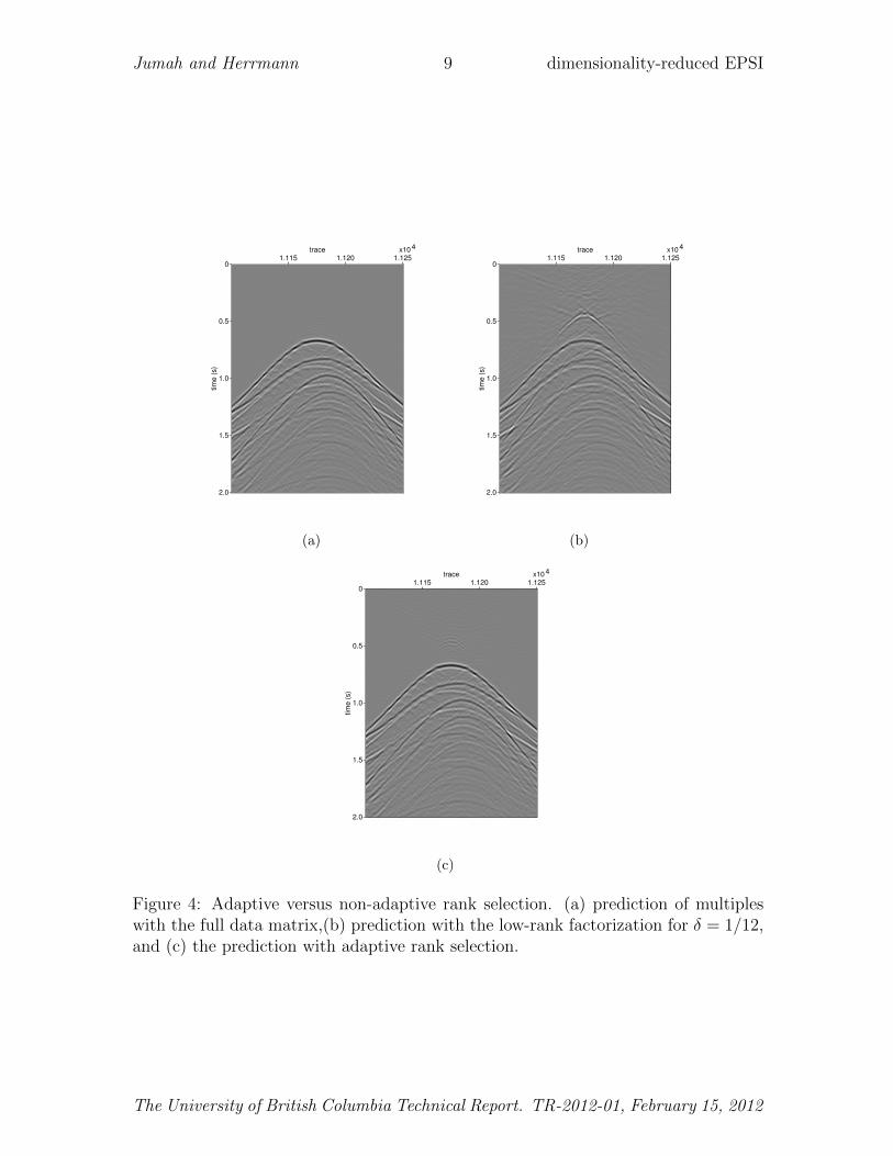
of this matrix is given by the rank k of the input data matrix P plus an oversamplingby p, typically set to 5−10. This operation is illustrated in Figure 5 and correspondsto forming p+ k amplitude encoded supershots by summing over all sequential shotswith random Gaussian weights (see e.g. van Leeuwen et al., 2011).

As long as the data matrix has a rank k or smaller this procedure obtains sufficientinformation to compute the SVD within a prescribed accuracy. To be more specific,the action on the random vectors gives us access to the range of the data matrix,which is spanned by the left vectors Q ∈ Cns×(k+p) of the QR factorization of Y.With these vectors, we form

Bns×(k+p) = Qns×(k+p)Pnr×ns , (9)

which is input to stage B, where we carry out the SVD on this reduced system. Theoperations that form stage A are summarized in Algorithm 1.

Algorithm 1 Randomized SVD

Input: Pnr×ns , a target rank k and the over-sampling parameter p

Output Orthonormal matrix Q whose range approximates the range of P

1. Draw a random Gaussian matrix Wns×(k+p).

2. Form Ynr×(k+p) = PW.

3. Construct the orthonormal matrix Qm×(k+p) by computing QR factorization ofY.



Figure 5: Supershots created by randomized superposition of sequential shots.

Stage B: computation of the low-rank factorization. The output of stage Acorresponds to a randomized dimensionality reduction capturing the action of thedata matrix from which we can now calculate the SVD with the advantage that weare working with a much smaller system. Following Halko et al. (2011), we compute

Bnr×k = Uk×kSk×kV∗k×ns

, (10)

from which we subsequently calculate the left singular vectors using the followingexpression

Unr×k = Qnr×kUk×k. (11)

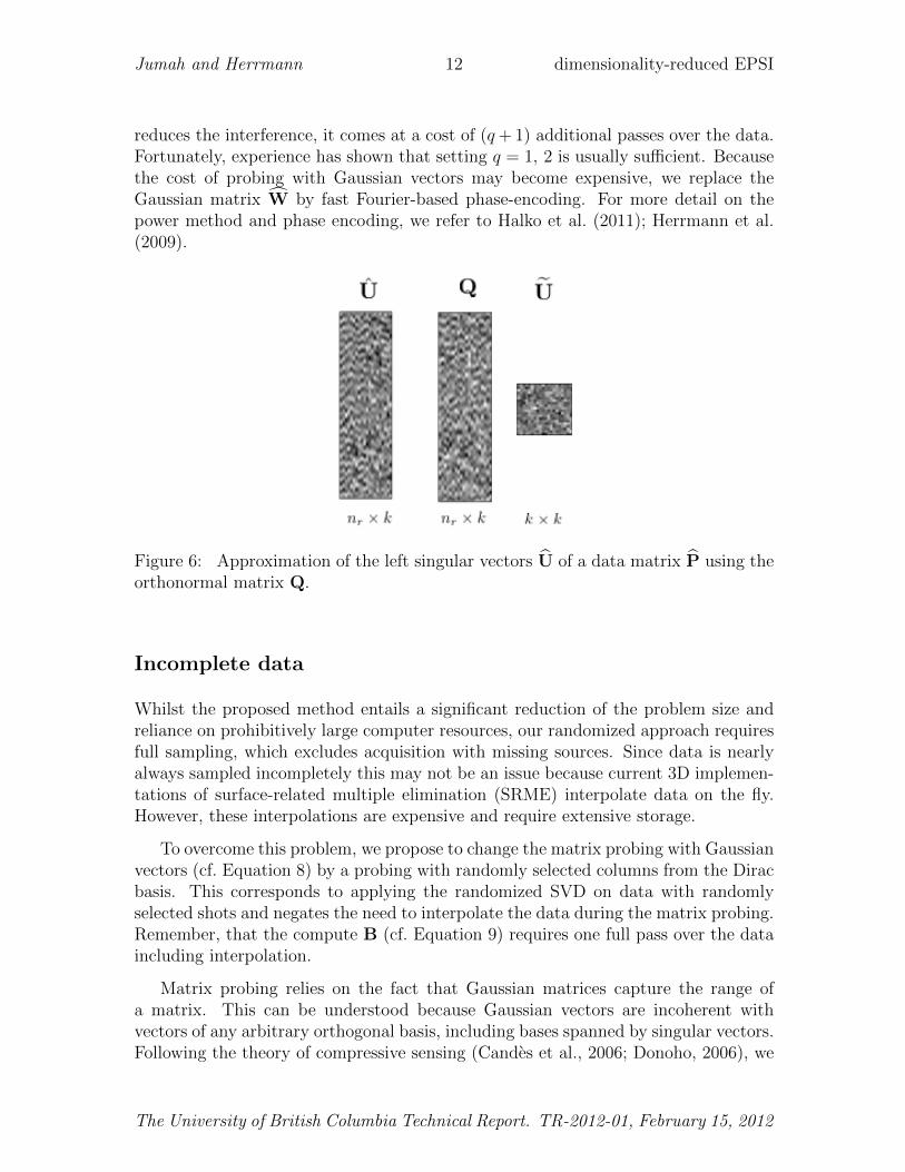
Figure 6, describes how the left singular vectors U of a data matrix P are computedusing the orthonormal matrix Q.

During this second stage, we factored the data matrix by carrying out the SVD onthe dimensionality reduced system. The advantage in this approach is that the fulldata matrix only needs to be accessed two times namely once for the action on therandom vectors to compute Y and once to form B. This is a significant improvementcompared to the k passes over the data required by the conventional SVD (see Halkoet al., 2011). However, the proposed Algorithm 1 is only appropriate for matricesthat have low rank or rapidly decaying singular values. Unfortunately, the algorithmwill perform poorly when approximating matrices that exhibit slow decay for theirsingular values (Halko et al., 2011). In that case, singular vectors associated with thesmall singular values are known to interfere with the approximation and this leads topoor quality of the approximation. To reduce these interferences, the decay for thesingular singular values can be improved by using the power method (Halko et al.,2011), which replaces Equation 8 by

B = (PP∗)qPW, (12)

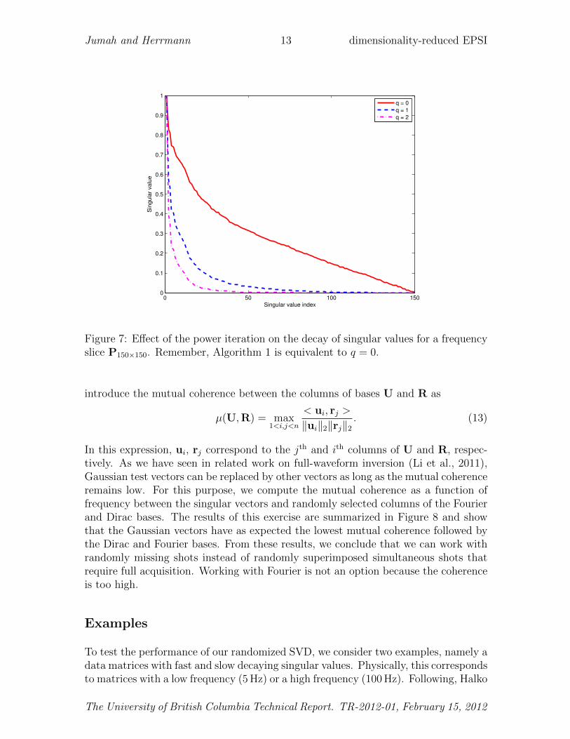
with q the order of the power. As a result of raising the matrix to the qth power,the singular values decay faster as illustrated in Figure 7. While this procedure



reduces the interference, it comes at a cost of (q+ 1) additional passes over the data.Fortunately, experience has shown that setting q = 1, 2 is usually sufficient. Becausethe cost of probing with Gaussian vectors may become expensive, we replace theGaussian matrix W by fast Fourier-based phase-encoding. For more detail on thepower method and phase encoding, we refer to Halko et al. (2011); Herrmann et al.(2009).

Figure 6: Approximation of the left singular vectors U of a data matrix P using theorthonormal matrix Q.

Incomplete data

Whilst the proposed method entails a significant reduction of the problem size andreliance on prohibitively large computer resources, our randomized approach requiresfull sampling, which excludes acquisition with missing sources. Since data is nearlyalways sampled incompletely this may not be an issue because current 3D implemen-tations of surface-related multiple elimination (SRME) interpolate data on the fly.However, these interpolations are expensive and require extensive storage.

To overcome this problem, we propose to change the matrix probing with Gaussianvectors (cf. Equation 8) by a probing with randomly selected columns from the Diracbasis. This corresponds to applying the randomized SVD on data with randomlyselected shots and negates the need to interpolate the data during the matrix probing.Remember, that the compute B (cf. Equation 9) requires one full pass over the dataincluding interpolation.

Matrix probing relies on the fact that Gaussian matrices capture the range ofa matrix. This can be understood because Gaussian vectors are incoherent withvectors of any arbitrary orthogonal basis, including bases spanned by singular vectors.Following the theory of compressive sensing (Candes et al., 2006; Donoho, 2006), we



0 50 100 1500

0.1

0.2

0.3

0.4

0.5

0.6

0.7

0.8

0.9

1

Singular value index

Sin

gu

lar

va

lue

q = 0

q = 1

q = 2

Figure 7: Effect of the power iteration on the decay of singular values for a frequencyslice P150×150. Remember, Algorithm 1 is equivalent to q = 0.

introduce the mutual coherence between the columns of bases U and R as

µ(U,R) = max1<i,j<n

< ui, rj >

‖ui‖2‖rj‖2. (13)

In this expression, ui, rj correspond to the jth and ith columns of U and R, respec-tively. As we have seen in related work on full-waveform inversion (Li et al., 2011),Gaussian test vectors can be replaced by other vectors as long as the mutual coherenceremains low. For this purpose, we compute the mutual coherence as a function offrequency between the singular vectors and randomly selected columns of the Fourierand Dirac bases. The results of this exercise are summarized in Figure 8 and showthat the Gaussian vectors have as expected the lowest mutual coherence followed bythe Dirac and Fourier bases. From these results, we conclude that we can work withrandomly missing shots instead of randomly superimposed simultaneous shots thatrequire full acquisition. Working with Fourier is not an option because the coherenceis too high.

Examples

To test the performance of our randomized SVD, we consider two examples, namely adata matrices with fast and slow decaying singular values. Physically, this correspondsto matrices with a low frequency (5 Hz) or a high frequency (100 Hz). Following, Halko



0 49 98 146 1950.2

0.25

0.3

0.35

0.4

0.45

0.5

0.55

Frequency (Hz)

Co

he

ren

ce

Fourier

Dirac

Gaussian

Figure 8: Coherence of the singular vectors of the data matrix with Fourier, Dirac, andGaussian bases for all frequencies.

et al. (2011) we compute the error for the k-rank approximation via

ek

= ‖(I−QQ∗)P‖S. (14)

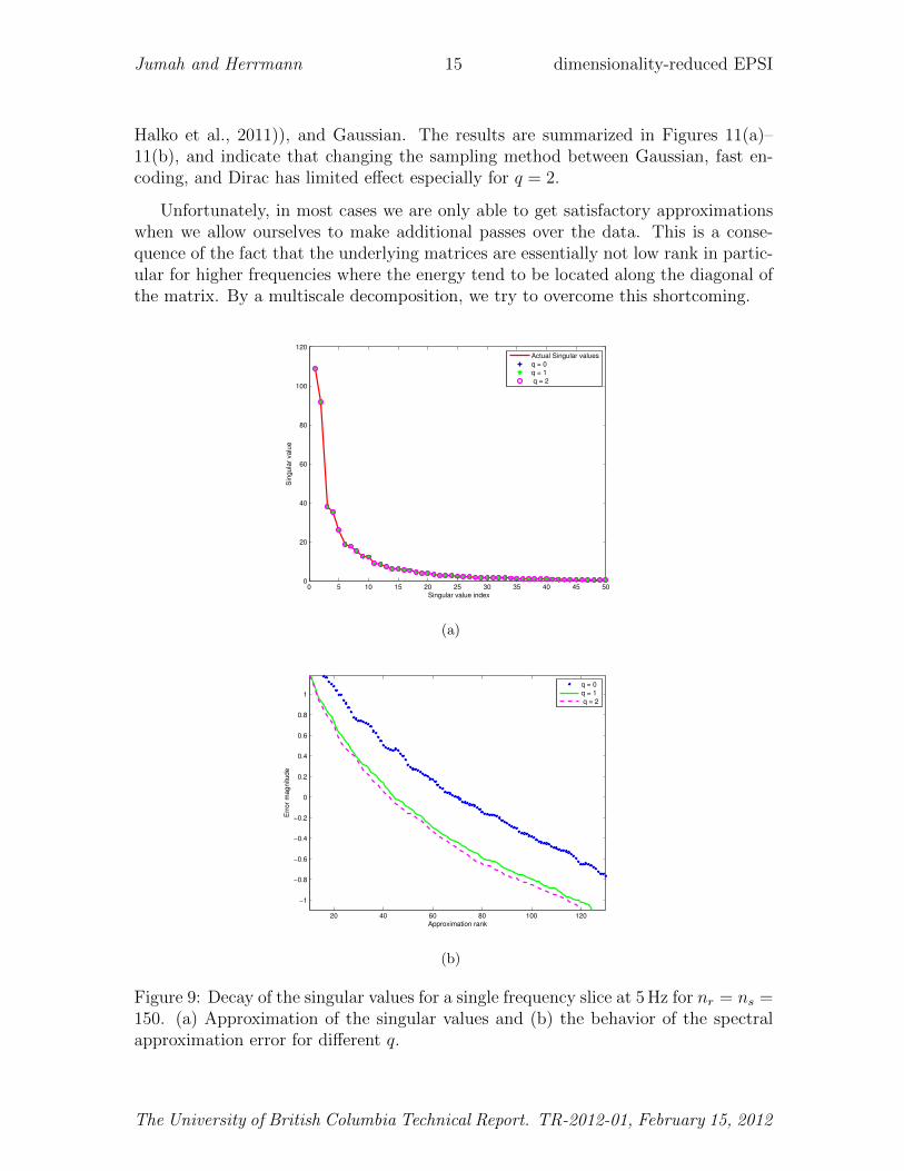
Fast decay: In this example, we apply the randomized SVD on a frequency slice at5 Hz from our synthetic dataset. Figure 9(a) contains the estimated singular valuesby matrix probing with Gaussian vectors for q = 0, 1, 2, and with k = 50. Fromthis plot, we observe that the singular values are estimated correctly for each q. Wealso observe from Figure 9(b) that the error given by the above equation is reducedsignificantly if we make at least one additional pass over the data—i.e., q > 0.

Slow decay: In this example, we apply the randomized SVD on the same dataset but at a high frequency of 100 Hz. In this case, we need an additional passover the data to get the accurate estimates for the singular values (see Figure 10(a).Unfortunately, Figure 10(b)) shows that the errors given by Equation 14 continue todecay slowly for increasing q. However, there is significant improvement compared tostandard probing (q = 0).

Different samplings: Finally, we compare the errors given by Equation 14 formatrix probing with Dirac, encoding with the subsampled Fourier transform (SRFT,



Halko et al., 2011)), and Gaussian. The results are summarized in Figures 11(a)–11(b), and indicate that changing the sampling method between Gaussian, fast en-coding, and Dirac has limited effect especially for q = 2.

Unfortunately, in most cases we are only able to get satisfactory approximationswhen we allow ourselves to make additional passes over the data. This is a conse-quence of the fact that the underlying matrices are essentially not low rank in partic-ular for higher frequencies where the energy tend to be located along the diagonal ofthe matrix. By a multiscale decomposition, we try to overcome this shortcoming.

0 5 10 15 20 25 30 35 40 45 500

20

40

60

80

100

120

Sin

gula

r valu

e


Actual Singular values

q = 0

q = 1

q = 2

(a)

20 40 60 80 100 120

−1

−0.8

−0.6

−0.4

−0.2

0

0.2

0.4

0.6

0.8

1

Approximation rank

Err

or

magnitude

q = 0

q = 1

q = 2

(b)

Figure 9: Decay of the singular values for a single frequency slice at 5 Hz for nr = ns =150. (a) Approximation of the singular values and (b) the behavior of the spectralapproximation error for different q.



0 5 10 15 20 25 30 35 40 45 50500

1000

1500

2000

2500

3000

3500


Sin

gula

r valu

e

Actual Singular values

q = 0

q = 1

q = 2

(a)

20 40 60 80 100 120

2.3

2.4

2.5

2.6

2.7

2.8

2.9

3

3.1

3.2

Approximation rank

Err

or

magnitude

q = 0

q = 1

q = 2

(b)

Figure 10: Decay of the singular values for a single frequency at 100 Hz for nr = ns =150. (a) Approximation of the singular values, and (b) the behavior of the spectralapproximation error.

10 20 30 40 50 60 70 80 90 100 110 120

−0.5

0

0.5

1

Approximation rank

Err

or

magnitude

Simultaneous Shots

Missing shots

SRFT

(a)

10 20 30 40 50 60 70 80 90 100 110 120

−1

−0.8

−0.6

−0.4

−0.2

0

0.2

0.4

0.6

0.8

Approximation rank

Err

or

magnitude

Simultaneous Shots

Missing shots

SRFT

(b)

Figure 11: Errors of the randomized SVD for different sampling methods (Gaussian,phase-encoded Fourier (SRFT), and Dirac (randomly-selected sequential shots), (a)approximation error using q = 0, and (b) approximation error for q = 2.



HIERARCHICALLY SEMI-SEPARABLE MATRIXREPRESENTATION

As we have seen in the previous section, data matrices become higher rank at higherfrequencies because the number of oscillations increase while the energy tends to fo-cus more around the diagonal. The latter property has to do with the increasedcurvature of seismic events as the frequency increases. While some recent theoreticalwork has been done to address this issue by including directionality in the formulation(Engquist and Ying, 2010), we rely on the Hierarchically Semi-Separable Matrix Rep-resentation (HSS, Chandrasekaran et al., 2006) in combination with the randomizedSVD along the lines of recent developments by Lin et al. (2011).

HSS matrices provide a way to represent high-rank structured dense matrices interms of low-rank submatrices with the aim of reducing the cost of linear algebraicoperations, e.g. reducing the cost of matrix-vector products from O(n2) to O(n). Aspart of the HSS representation, matrices are recursively repartitioned into high-rankdiagonal and low-rank off-diagonal matrixes. SVDs are carried on the off diagonalsubmatrices while the high-rank diagonal submatrices are recursively partitioned tosome user defined level, which depends on the desirable compression and accuracy.With this decomposition, HSS is able to carry out fast matrix operations (Chan-drasekaran et al., 2006).

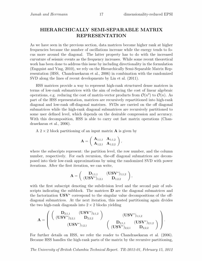
A 2× 2 block partitioning of an input matrix A is given by

A =

(A1;1,1 A1;1,2

A1;2,1 A1;2,2

),

where the subscripts represent: the partition level, the row number, and the columnnumber, respectively. For each recursion, the-off diagonal submatrices are decom-posed into their low-rank approximations by using the randomized SVD with poweriterations. After the first iteration, we can write,

A =

(D1;1,1 (USV∗)1;1,2

(USV∗)1;2,1 D1;2,2

),

with the first subscript denoting the subdivision level and the second pair of sub-scripts indicating the subblock. The matrices D are the diagonal submatrices andthe factorization USV∗ correspond to the singular value decompositions of the off-diagonal submatrices. At the next iteration, this nested partitioning again dividesthe two high-rank diagonals into 2× 2 blocks yielding

A =

(

D2;1,1 (USV∗)2;1,2(USV∗)2;2,1 D2;2,2

)(USV∗)1;1,2

(USV∗)1;2,1

(D2;1,1 (USV∗)2;1,2

(USV∗)2;2,1 D2;2,2

) .

For further details on HSS, we refer the reader to Chandrasekaran et al. (2006).Because HSS handles the high-rank parts of the matrix by the recursive partitioning,



we end up with an algorithm that only requires a few passes over the data. We achievethis by carrying out the matrix probing on each low-rank submatrix separately whileleaving the high-rank diagonal matrices at the fines level alone. This approach has theadvantage of increasing the decay of the singular for the low-rank submatrices, whichis beneficial to the matrix probing. In addition, the algorithm does not need to storethe singular vectors for the coarse low-rank decompositions. Instead, the algorithmcomputes the singular vectors at the lower level of the decomposition recursively fromthe singular vectors at the finer level Chandrasekaran et al. (2006). To determine theproper rank for the matrix probing, we use Algorithm 4.2 from Halko et al. (2011).

Example

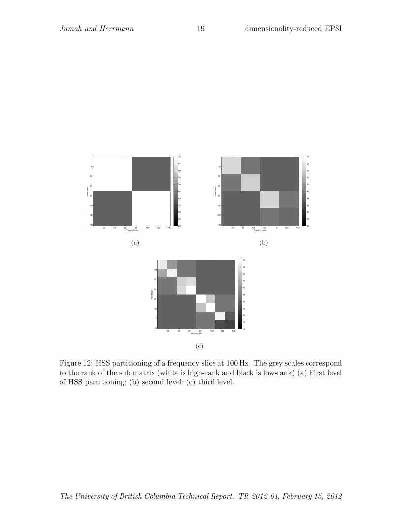
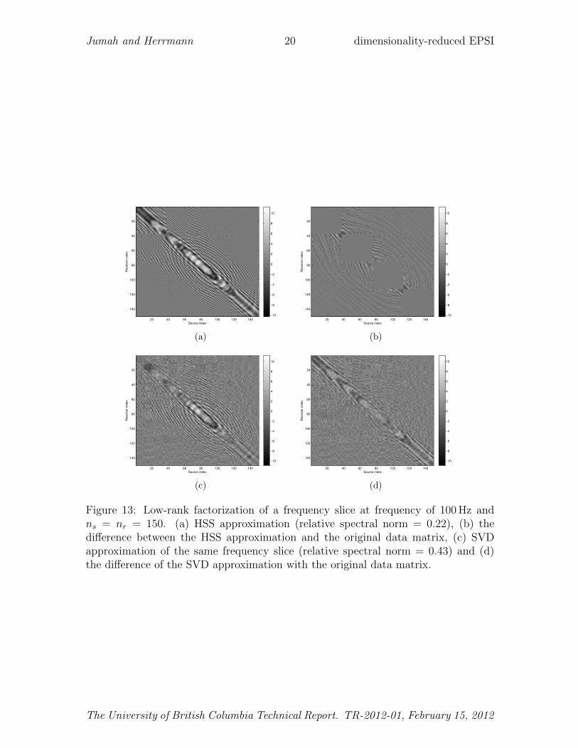
To demonstrate the effectiveness of the HSS representation, we consider a monochro-matic frequency slice at 100 Hz, which we approximate with a three-level HSS rep-resentation in combination with our randomized SVD with adaptive rank selection.Before applying this algorithm, we first verify the anticipated behavior of the HSSblocks in Figure 12, which shows that the rank of the off-diagonal subblocks is indeedlower than the rank of the diagonal subblocks. This justifies the use of HSS on high-frequency data matrices. As we can see from Figure 13, the HSS-based factorizationattains a better approximation, which is reflected in the spectral norms shown in thegrey-scale plots.

APPLICATION TO SYNTHETIC AND REAL DATA

To establish the performance of our method, we compare the output of EPSI (Linand Herrmann, 2011) with the output of EPSI using low-rank approximations forthe data matrix. Depending on the ratio between the largest singular value of aparticular data matrix and the largest singular amongst all data matrices, we eitherproceed by applying the randomized SVD or we first apply the HSS partitioning priorto the computation of the randomized SVDs on the off diagonals. We conduct twoexperiments and we fix the subsampling ratios to δ = [1/2, 1/5, 1/8, 1/12].

Synthetic data

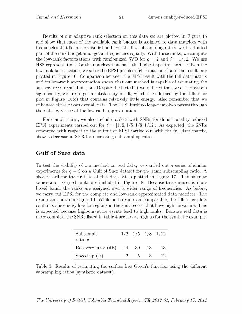
In this example, we use data modeled from a velocity model that consists of a high-velocity layer, which represents salt, surrounded by sedimentary layers and a waterbottom that is not completely flat (see Herrmann et al., 2007). Using an acousticfinite-difference modeling algorithm, 150 shots with 150 receivers are simulated on afixed receiver spread. A shot record for the first 2 s with surface-related multiples isplotted in Figure 14. For a plot of the singular values of this synthetic data sets, referto Figure 3.



Column Index

Row

Index

20 40 60 80 100 120 140

20

40

60

80

100

120

14020

25

30

35

40

45

50

55

60

65

70

(a)

Column Index

Row

Index

20 40 60 80 100 120 140

20

40

60

80

100

120

14020

25

30

35

40

45

50

55

60

65

70

(b)

Column Index

Row

Index

20 40 60 80 100 120 140

20

40

60

80

100

120

14020

25

30

35

40

45

50

55

60

65

70

(c)

Figure 12: HSS partitioning of a frequency slice at 100 Hz. The grey scales correspondto the rank of the sub matrix (white is high-rank and black is low-rank) (a) First levelof HSS partitioning; (b) second level; (c) third level.



Source index

Re

ce

ive

r in

de

x

20 40 60 80 100 120 140

20

40

60

80

100

120

140

−10

−8

−6

−4

−2

0

2

4

6

8

10

(a)

Source index

Re

ce

ive

r in

de

x

20 40 60 80 100 120 140

20

40

60

80

100

120

140

−10

−8

−6

−4

−2

0

2

4

6

8

10

(b)

Source index

Re

ce

ive

r in

de

x

20 40 60 80 100 120 140

20

40

60

80

100

120

140

−10

−8

−6

−4

−2

0

2

4

6

8

10

(c)

Source index

Re

ce

ive

r in

de

x

20 40 60 80 100 120 140

20

40

60

80

100

120

140

−10

−8

−6

−4

−2

0

2

4

6

8

10

(d)

Figure 13: Low-rank factorization of a frequency slice at frequency of 100 Hz andns = nr = 150. (a) HSS approximation (relative spectral norm = 0.22), (b) thedifference between the HSS approximation and the original data matrix, (c) SVDapproximation of the same frequency slice (relative spectral norm = 0.43) and (d)the difference of the SVD approximation with the original data matrix.



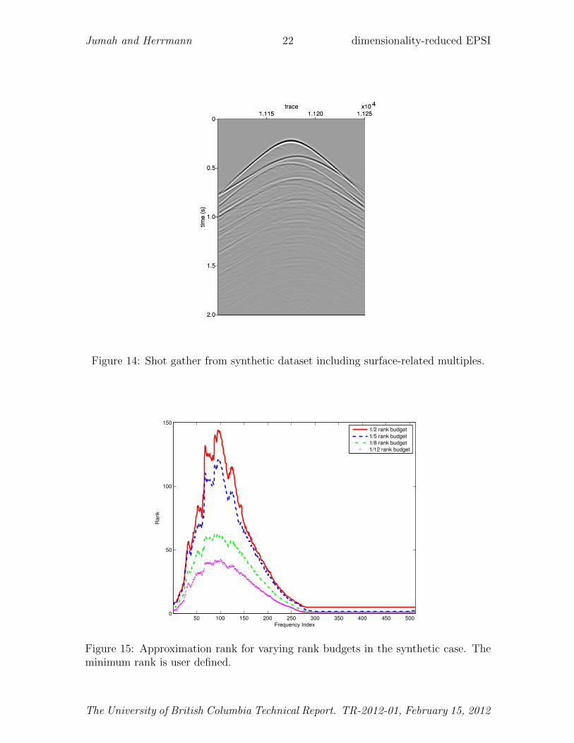
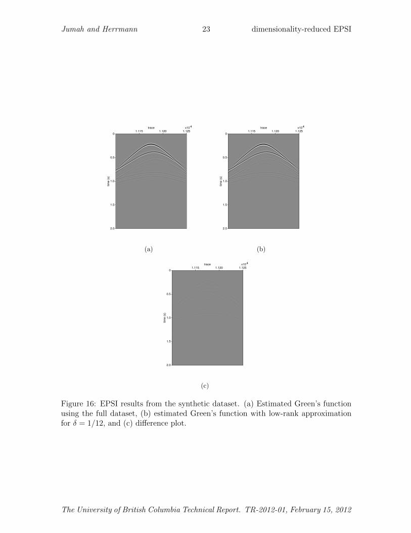
Results of our adaptive rank selection on this data set are plotted in Figure 15and show that most of the available rank budget is assigned to data matrices withfrequencies that lie in the seismic band. For the low subsampling ratios, we distributedpart of the rank budget amongst all frequencies equally. With these ranks, we computethe low-rank factorizations with randomized SVD for q = 2 and δ = 1/12. We useHSS representations for the matrices that have the highest spectral norm. Given thelow-rank factorization, we solve the EPSI problem (cf. Equation 4) and the results areplotted in Figure 16. Comparison between the EPSI result with the full data matrixand its low-rank approximation shows that our method is capable of estimating thesurface-free Green’s function. Despite the fact that we reduced the size of the systemsignificantly, we are to get a satisfactory result, which is confirmed by the differenceplot in Figure. 16(c) that contains relatively little energy. Also remember that weonly need three passes over all data. The EPSI itself no longer involves passes throughthe data by virtue of the low-rank approximation.

For completeness, we also include table 3 with SNRs for dimensionality-reducedEPSI experiments carried out for δ = [1/2, 1/5, 1/8, 1/12]. As expected, the SNRscomputed with respect to the output of EPSI carried out with the full data matrix,show a decrease in SNR for decreasing subsampling ratios.

Gulf of Suez data

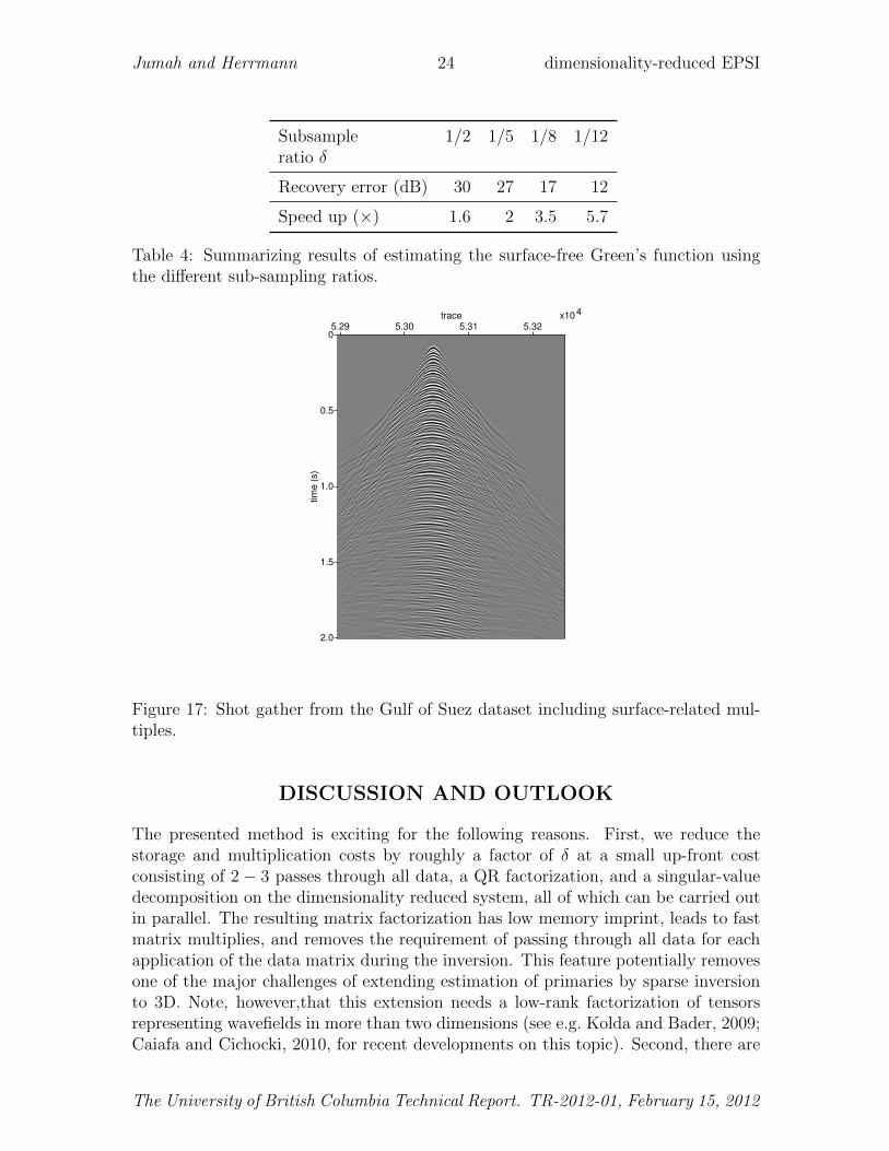
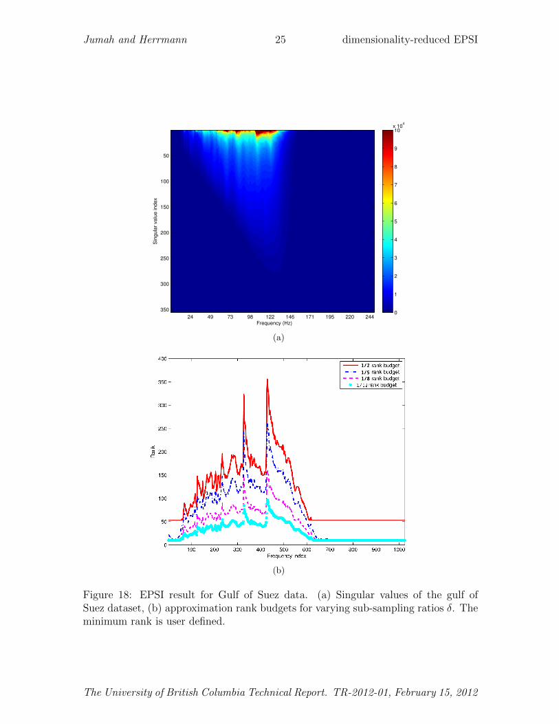
To test the viability of our method on real data, we carried out a series of similarexperiments for q = 2 on a Gulf of Suez dataset for the same subsampling ratio. Ashot record for the first 2 s of this data set is plotted in Figure 17. The singularvalues and assigned ranks are included in Figure 18. Because this dataset is morebroad band, the ranks are assigned over a wider range of frequencies. As before,we carry out EPSI for the complete and low-rank approximated data matrices. Theresults are shown in Figure 19. While both results are comparable, the difference plotscontain some energy loss for regions in the shot record that have high curvature. Thisis expected because high-curvature events lead to high ranks. Because real data ismore complex, the SNRs listed in table 4 are not as high as for the synthetic example.

Subsample 1/2 1/5 1/8 1/12ratio δ

Recovery error (dB) 44 30 18 13

Speed up (×) 2 5 8 12

Table 3: Results of estimating the surface-free Green’s function using the differentsubsampling ratios (synthetic dataset).



Figure 14: Shot gather from synthetic dataset including surface-related multiples.

50 100 150 200 250 300 350 400 450 5000

50

100

150

Frequency Index

Rank

1/2 rank budget

1/5 rank budget

1/8 rank budget

1/12 rank budget

Figure 15: Approximation rank for varying rank budgets in the synthetic case. Theminimum rank is user defined.



0

0.5

1.0

1.5

2.0

tim

e (

s)

1.115 1.120 1.125x104trace

(a)

0

0.5

1.0

1.5

2.0

tim

e (

s)

1.115 1.120 1.125x104trace

(b)

0

0.5

1.0

1.5

2.0

tim

e (

s)

1.115 1.120 1.125x104trace

(c)

Figure 16: EPSI results from the synthetic dataset. (a) Estimated Green’s functionusing the full dataset, (b) estimated Green’s function with low-rank approximationfor δ = 1/12, and (c) difference plot.



Subsample 1/2 1/5 1/8 1/12ratio δ

Recovery error (dB) 30 27 17 12

Speed up (×) 1.6 2 3.5 5.7

Table 4: Summarizing results of estimating the surface-free Green’s function usingthe different sub-sampling ratios.

0

0.5

1.0

1.5

2.0

tim

e (

s)

5.29 5.30 5.31 5.32x104trace

Figure 17: Shot gather from the Gulf of Suez dataset including surface-related mul-tiples.

DISCUSSION AND OUTLOOK

The presented method is exciting for the following reasons. First, we reduce thestorage and multiplication costs by roughly a factor of δ at a small up-front costconsisting of 2 − 3 passes through all data, a QR factorization, and a singular-valuedecomposition on the dimensionality reduced system, all of which can be carried outin parallel. The resulting matrix factorization has low memory imprint, leads to fastmatrix multiplies, and removes the requirement of passing through all data for eachapplication of the data matrix during the inversion. This feature potentially removesone of the major challenges of extending estimation of primaries by sparse inversionto 3D. Note, however,that this extension needs a low-rank factorization of tensorsrepresenting wavefields in more than two dimensions (see e.g. Kolda and Bader, 2009;Caiafa and Cichocki, 2010, for recent developments on this topic). Second, there are



Frequency (Hz)

Sin

gula

r valu

e index

24 49 73 98 122 146 171 195 220 244

50

100

150

200

250

300

3500

1

2

3

4

5

6

7

8

9

10x 10

4

(a)

(b)

Figure 18: EPSI result for Gulf of Suez data. (a) Singular values of the gulf ofSuez dataset, (b) approximation rank budgets for varying sub-sampling ratios δ. Theminimum rank is user defined.



0

0.5

1.0

1.5

2.0

2.5

tim

e (

s)

5.29 5.30 5.31 5.32x104trace

(a)

0

0.5

1.0

1.5

2.0

2.5

tim

e (

s)

5.29 5.30 5.31 5.32x104trace

(b)

0

0.5

1.0

1.5

2.0

tim

e (

s)

5.29 5.30 5.31 5.32x104trace

(c)

Figure 19: EPSI result for the gulf of Suez dataset. (a) Estimated Green’s functionwith the full data matrix, (b) estimated Green’s function for low-rank approximationfor δ = 1/12, and (c) difference plot.



connections between matrix probing and simultaneous sourcing during acquisitionof marine data (Wason et al., 2011) or during imaging and full-waveform inversion(Herrmann et al., 2009). This opens the possibility to further speed up our algorithms(see e.g. Herrmann, 2010; van Leeuwen et al., 2011) or to work with simultaneouslyacquired data directly. Third, because the singular vectors of the data matrix areincoherent with the Dirac basis, we can limit the need of interpolating the data toonly once as part of the second stage during which the singular-value decompositionis conducted. In case the locations of the missing shots are sufficiently randomlydistributed, we showed that it is no longer necessary to interpolate the data as partof the matrix probing. Instead, we can consider data with randomly missing shotsas the result of the matrix probing. Needless to say, this could lead to significantcost savings. Fourth, the proposed algorithm is relatively simple, requires matrix-free application (read ’black-box’ implementations of SRME (Verschuur et al., 1992;Berkhout and Verschuur, 1997; Weglein et al., 1997))) of the data matrix only, andlimits the number of passes through the data. This may lead to significant speedupbecause the method only requires a few on-the-fly interpolations. Fifth, our low-rank approximations of the data matrix allows us to leverage recent extensions ofcompressive sensing to matrix-completion problems (Candes and Recht, 2009; Gandyet al., 2011) where matrices or tensors are reconstructed from incomplete data (readdata with missing traces). In these formulations, data is regularized solving thefollowing optimization problem

X = arg minX

‖X‖∗ subject to ‖A(X)− b‖2 ≤ σ, (15)

with ‖ · ‖∗ =∑|λi| the nuclear norm summing the magnitudes of the singular values

(λ) of the matrix X. Here, A(·) a linear operator that samples the data matrix. Itcan be shown that this program is a convex relaxation of finding the matrix X withthe smallest rank given incomplete data. Finally, low-rank approximations for tensorswere recently proposed by Oropeza and Sacchi (2010) for seismic denoising. Sixth,the singular vectors of our low-rank approximation can also be used in imaging orfull-waveform inversion Habashy et al. (2010).

CONCLUSIONS

Data-driven methods—such as the estimation of primaries by sparse inversion—sufferfrom the ’curse of dimensionality’ because these methods require repeated applica-tions of the data matrix whose size grows exponentially with the dimension. In thispaper, we leverage recent developments in dimensionality reduction that allow usto approximate the action of the data matrix via a low-rank matrix factorizationbased on the randomized singular-value decomposition. Combination of this methodwith hierarchical semi-separable matrix representations enabled us to efficiently factorhigh-frequency data matrices that have relative high ranks. The resulting low-rankfactorizations of the data matrices lead to significant reductions in storage and matrixmultiplication costs. The reduction in costs for the low-rank approximations them-selves are, by virtue of the randomization, cheap and only require a limited number



of applications of the full data matrix to random vectors. This operation can easilybe carried out in parallel using existing code bases for surface-related multiple pre-diction and can lead to significant speedups and reductions in memory use. Becausethe singular vectors of the data matrices are incoherent with the Dirac basis, matrixprobing by Gaussian vectors that require on-the-fly interpolations can be replaced bymatrix probings consisting of data with missing shots. As a consequence, the num-ber of interpolations is reduced to only one and this could give rise to a significantimprovement in the performance of the inversion, which typically requires severalapplications of the data matrix.

ACKNOWLEDGMENTS

We would like to thank the authors of SPOT (http://www.cs.ubc.ca/labs/scl/spot/), SPG`1 (http://www.cs.ubc.ca/labs/scl/spgl1/), CurveLab (curvelet.org), and the MSN toolbox for the HSS matrices (http://scg.ece.ucsb.edu/msn.html). We also would like to thank Tim Lin for providing us with the code for EPSI.This paper was prepared with Madagascar (rsf.sf.net) and was in part financiallysupported by by the CRD Grant DNOISE 334810-05. The industrial sponsors ofthe Seismic Laboratory for Imaging and Modelling (SLIM) BG Group, BP, BGP,BP, Chevron, ConocoPhillips, Petrobras, PGS, Total SA., and WesternGeco are alsogratefully acknowledged.

REFERENCES

Berkhout, A. J., and Y.-H. Pao, 1982, Seismic migration—imaging of acoustic energyby wave field extrapolation: Journal of Applied Mechanics, 49, 682–683.

Berkhout, A. J., and D. J. Verschuur, 1997, Estimation of multiple scattering byiterative inversion, part I: theoretical considerations: Geophysics, 62, 1586–1595.

Caiafa, C. F., and A. Cichocki, 2010, Generalizing the column-row matrix decompo-sition to multi-way arrays: Linear Algebra and its Applications, 433, 557 – 573.

Candes, E., and B. Recht, 2009, Exact matrix completion via convex optimization:Foundations of Computational Mathematics, 9, 717–772.

Candes, E. J., J. Romberg, and T. Tao, 2006, Stable signal recovery from incompleteand inaccurate measurements: 59, 1207–1223.

Chandrasekaran, S., P. Dewilde, M. Gu, W. Lyons, and T. Pals, 2006, A fast solverfor hss representations via sparse matrices.: SIAM J. Matrix Analysis Applications,29, 67–81.

Chiu, J., and L. Demanet, 2012, Sublinear randomized algorithms for skeleton de-compositions.

Dedem, E., 2002, 3D surface-related multiple prediction: PhD thesis. (Delft Univer-sity of Technology).

Demanet, L., P.-D. Letourneau, N. Boumal, H. Calandra, J. Chiu, and S. Snelson,


http://www.cs.ubc.ca/labs/scl/spot/

http://www.cs.ubc.ca/labs/scl/spot/

http://www.cs.ubc.ca/labs/scl/spgl1/

curvelet.org

curvelet.org

http://scg.ece.ucsb.edu/msn.html

http://scg.ece.ucsb.edu/msn.html

rsf.sf.net

http://slim.eos.ubc.ca/?module=articles&func=display&catid=43&aid=100

slim.eos.ubc.ca

http://www.bg-group.com/

http://www.bp.com/

http://www.bgp.com.cn/

http://www.bp.com/

http://www.chevron.com/

http://www.conocophillips.com/

http://www.petrobras.com/

http://www.pgs.com/

http://www.total.com/

http://www.westerngeco.com/


2012, Matrix probing: a randomized preconditioner for the wave-equation Hessian:Journal of Apllied Computational Harmonic Analysis, 32, 155–168.

Donoho, D. L., 2006, Compressed sensing: IEEE Trans. Inform. Theory, 52, 1289–1306.

Engquist, B., and L. Ying, 2010, Fast directional algorithms for the Helmholtz kernel:Journal of Computational and Applied Mathematics, 234, 1851 – 1859.

Gandy, S., B. Recht, and I. Yamada, 2011, Tensor completion and low-n-rank tensorrecovery via convex optimization: Inverse Problems, 27, 025010.

Habashy, T. M., A. Abubakar, G. Pan, and A. Belani, 2010, Full-waveform seismicinversion using the source-receiver compression approach: SEG Technical ProgramExpanded Abstracts, SEG, 1023–1028.

Halko, N., P. G. Martinsson, and J. A. Tropp, 2011, Finding structure with random-ness: Probabilistic algorithms for constructing approximate matrix decompositions:SIAM Rev., 53, no. 2, 217–288.

Herrmann, F. J., 2010, Randomized sampling and sparsity: Getting more informationfrom fewer samples: Geophysics, 75, WB173–WB187.

Herrmann, F. J., U. Boeniger, and D. J. Verschuur, 2007, Non-linear primary-multipleseparation with directional curvelet frames: Geophysical Journal International,170, 781–799.

Herrmann, F. J., Y. A. Erlangga, and T. Lin, 2009, Compressive simultaneous full-waveform simulation: Geophysics, 74, A35.

Kolda, T. G., and B. W. Bader, 2009, Tensor decompositions and applications: SIAMReview, 51, 455–500.

Li, X., A. Y. Aravkin, T. van Leeuwen, and F. J. Herrmann, 2011, Fast randomizedfull-waveform inversion with compressive sensing. to appear in Geophysics.

Lin, L., J. Lu, and L. Ying, 2011, Fast construction of hierarchical matrix represen-tation from matrix-vector multiplication: Journal of Computational Physics, 230,4071 – 4087.

Lin, T. T., and F. J. Herrmann, 2011, Estimating primaries by sparse inversion ina curvelet-like representation domain: Presented at the 73th Ann. Internat. Mtg.,EAGE, Eur. Ass. of Geosc. and Eng., Expanded abstracts.

Lin, T. T. Y., and F. J. Herrmann, 2012, Robust estimation of primaries by sparseinversion via `1 minimization. (in preparation).

Minato, S., T. Matsuoka, T. Tsuji, D. Draganov, J. Hunziker, and K. Wapenaar,2011, Seismic interferometry using multidimensional deconvolution and crosscorre-lation for crosswell seismic reflection data without borehole sources: Geophysics,76, SA19–SA34.

Oropeza, V. E., and M. D. Sacchi, 2010, A randomized SVD for multichannel singularspectrum analysis (MSSA) noise attenuation: SEG, Expanded Abstracts, 29, 3539–3544.

van Groenestijn, G. J. A., and D. J. Verschuur, 2009, Estimating primaries by sparseinversion and application to near-offset data reconstruction: Geophysics, 74, A23–A28.

van Leeuwen, T., A. Aravkin, and F. J. Herrmann, 2011, Seismic waveform inversionby stochastic optimization: International Journal of Geophysics, 689041.



Verschuur, D. J., A. J. Berkhout, and C. P. A. Wapenaar, 1992, Adaptive surface-related multiple elimination: Geophysics, 57, 1166–1177.

Wason, H., F. J. Herrmann, and T. T. Lin, 2011, Sparsity-promoting recovery fromsimultaneous data: a compressive sensing approach: SEG Technical Program Ex-panded Abstracts, SEG, 6–10.

Weglein, A. B., F. A. Carvalho, and P. M. Stolt, 1997, An iverse scattering seriesmethod for attenuating multiples in seismic reflection data: Geophysics, 62, 1975–1989.


dimensionality-reduced estimation of primaries by · pdf fileazimuth seismic recording and...

Documents