digital signal processingquizzes q1 write the recursive equation for the ks algorithm q2 a major...
TRANSCRIPT
Digital Signal Processing
Module 2: Discrete-time signalsDigital Signal Processing
Paolo Prandoni and Martin Vetterli
© 2013

Video Introduction
Digital Signal Processing
Paolo Prandoni and Martin Vetterli
© 2013

Module Overview:
◮ Module 2.1: discrete-time signals and operators
◮ Module 2.2: the discrete-time complex exponential
◮ Module 2.3: the Karplus-Strong algorithm
2 1
Digital Signal Processing
Paolo Prandoni and Martin Vetterli
© 2013

Digital Signal Processing
Module 2.1: Discrete-time signalsDigital Signal Processing
Paolo Prandoni and Martin Vetterli
© 2013

Overview:
◮ discrete-time signals
◮ signal classes
◮ elementary operators
◮ shifts
◮ energy and power
2.1 2
Digital Signal Processing
Paolo Prandoni and Martin Vetterli
© 2013

Discrete-time signals
Economics: the Dow Jones industrial average
0
5000
10000
1891 1916 1941 1966 1991 2016
year
2.1 3
Digital Signal Processing
Paolo Prandoni and Martin Vetterli
© 2013
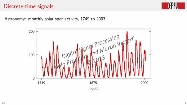
Discrete-time signals
Astronomy: monthly solar spot activity, 1749 to 2003
1749 1875 20000
100
200
month
2.1 4
Digital Signal Processing
Paolo Prandoni and Martin Vetterli
© 2013

Discrete-time signals
History: world population (billions)
1AD 1700AD 2030AD0
1
2
3
4
5
6
7
8
9
year
2.1 5
Digital Signal Processing
Paolo Prandoni and Martin Vetterli
© 2013

Discrete-time signals have a long tradition...
Meteorology (limnology): the floods of the Nile
Representations of flood data: circa 2500 BC and today
2.1 6
Digital Signal Processing
Paolo Prandoni and Martin Vetterli
© 2013
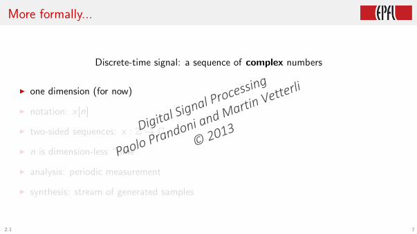
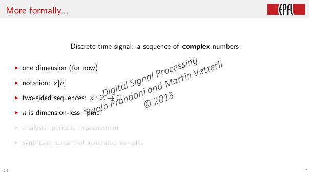
More formally...
Discrete-time signal: a sequence of complex numbers
◮ one dimension (for now)
◮ notation: x [n]
◮ two-sided sequences: x : Z → C
◮ n is dimension-less “time”
◮ analysis: periodic measurement
◮ synthesis: stream of generated samples
2.1 7
Digital Signal Processing
Paolo Prandoni and Martin Vetterli
© 2013

The delta signal
x [n] = δ[n]
b b b b b b b b b b b b b b b b
b
b b b b b b b b b b b b b b b b
−15 −10 −5 0 5 10 150
1
2.1 8
Digital Signal Processing
Paolo Prandoni and Martin Vetterli
© 2013
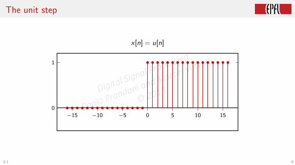
The unit step
x [n] = u[n]
b b b b b b b b b b b b b b b b
b b b b b b b b b b b b b b b b b
−15 −10 −5 0 5 10 150
1
2.1 9
Digital Signal Processing
Paolo Prandoni and Martin Vetterli
© 2013
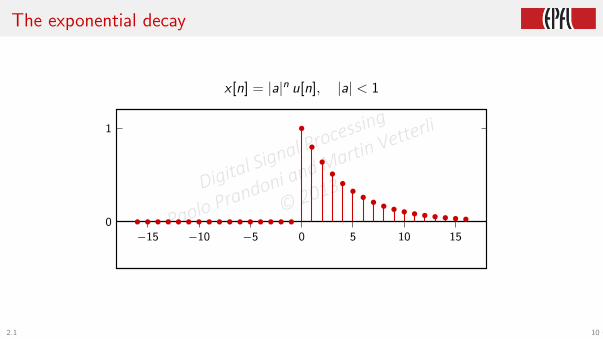
The exponential decay
x [n] = |a|n u[n], |a| < 1
b b b b b b b b b b b b b b b b
b
b
bbbbb b b b b b b b b b b
−15 −10 −5 0 5 10 150
1
2.1 10
Digital Signal Processing
Paolo Prandoni and Martin Vetterli
© 2013

The sinusoid
x [n] = sin(ω0n + θ)
b
b
b
b
bb b b
b
b
b
b
b
b
bb b b
b
b
b
b
b
b
bb b b
b
b
b
b
b
−15 −10 −5 0 5 10 15
−1
0
1
2.1 11
Digital Signal Processing
Paolo Prandoni and Martin Vetterli
© 2013

Four signal classes
◮ finite-length
◮ infinite-length
◮ periodic
◮ finite-support
2.1 12
Digital Signal Processing
Paolo Prandoni and Martin Vetterli
© 2013

Four signal classes
◮ finite-length
◮ infinite-length
◮ periodic
◮ finite-support
2.1 12
Digital Signal Processing
Paolo Prandoni and Martin Vetterli
© 2013

Four signal classes
◮ finite-length
◮ infinite-length
◮ periodic
◮ finite-support
2.1 12
Digital Signal Processing
Paolo Prandoni and Martin Vetterli
© 2013

Four signal classes
◮ finite-length
◮ infinite-length
◮ periodic
◮ finite-support
2.1 12
Digital Signal Processing
Paolo Prandoni and Martin Vetterli
© 2013
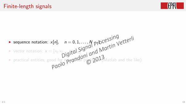
Finite-length signals
◮ sequence notation: x [n], n = 0, 1, . . . ,N − 1
◮ vector notation: x = [x0 x1 . . . xN−1]T
◮ practical entities, good for numerical packages (Matlab and the like)
2.1 13
Digital Signal Processing
Paolo Prandoni and Martin Vetterli
© 2013

Finite-length signals
◮ sequence notation: x [n], n = 0, 1, . . . ,N − 1
◮ vector notation: x = [x0 x1 . . . xN−1]T
◮ practical entities, good for numerical packages (Matlab and the like)
2.1 13
Digital Signal Processing
Paolo Prandoni and Martin Vetterli
© 2013

Finite-length signals
◮ sequence notation: x [n], n = 0, 1, . . . ,N − 1
◮ vector notation: x = [x0 x1 . . . xN−1]T
◮ practical entities, good for numerical packages (Matlab and the like)
2.1 13
Digital Signal Processing
Paolo Prandoni and Martin Vetterli
© 2013

Infinite-length signals
◮ sequence notation: x [n], n ∈ Z
◮ abstraction, good for theorems
2.1 14
Digital Signal Processing
Paolo Prandoni and Martin Vetterli
© 2013

Infinite-length signals
◮ sequence notation: x [n], n ∈ Z
◮ abstraction, good for theorems
2.1 14
Digital Signal Processing
Paolo Prandoni and Martin Vetterli
© 2013

Periodic signals
◮ N-periodic sequence: x̃ [n] = x̃ [n + kN], n, k ,N ∈ Z
◮ same information as finite-length of length N
◮ “natural” bridge between finite and infinite lengths
2.1 15
Digital Signal Processing
Paolo Prandoni and Martin Vetterli
© 2013

Periodic signals
◮ N-periodic sequence: x̃ [n] = x̃ [n + kN], n, k ,N ∈ Z
◮ same information as finite-length of length N
◮ “natural” bridge between finite and infinite lengths
2.1 15
Digital Signal Processing
Paolo Prandoni and Martin Vetterli
© 2013

Periodic signals
◮ N-periodic sequence: x̃ [n] = x̃ [n + kN], n, k ,N ∈ Z
◮ same information as finite-length of length N
◮ “natural” bridge between finite and infinite lengths
2.1 15
Digital Signal Processing
Paolo Prandoni and Martin Vetterli
© 2013
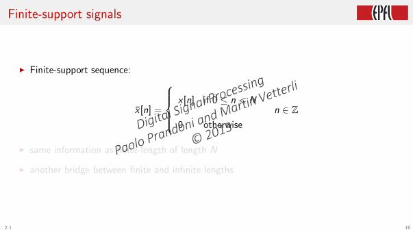
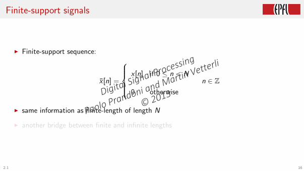
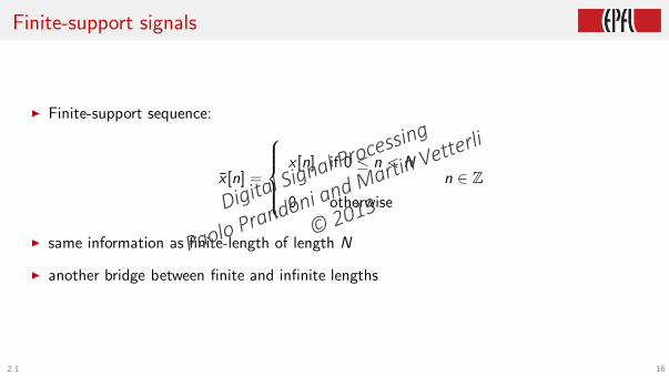
Finite-support signals
◮ Finite-support sequence:
x̄ [n] =
x [n] if 0 ≤ n < N
0 otherwise
n ∈ Z
◮ same information as finite-length of length N
◮ another bridge between finite and infinite lengths
2.1 16
Digital Signal Processing
Paolo Prandoni and Martin Vetterli
© 2013
Finite-support signals
◮ Finite-support sequence:
x̄ [n] =
x [n] if 0 ≤ n < N
0 otherwise
n ∈ Z
◮ same information as finite-length of length N
◮ another bridge between finite and infinite lengths
2.1 16
Digital Signal Processing
Paolo Prandoni and Martin Vetterli
© 2013
Finite-support signals
◮ Finite-support sequence:
x̄ [n] =
x [n] if 0 ≤ n < N
0 otherwise
n ∈ Z
◮ same information as finite-length of length N
◮ another bridge between finite and infinite lengths
2.1 16
Digital Signal Processing
Paolo Prandoni and Martin Vetterli
© 2013

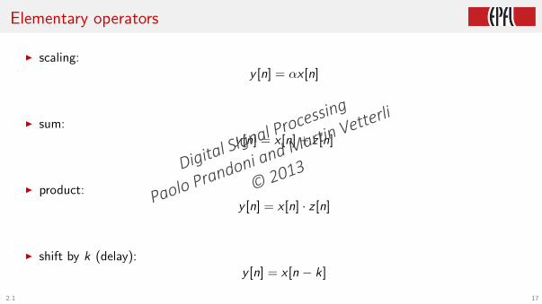
Elementary operators
◮ scaling:y [n] = αx [n]
◮ sum:y [n] = x [n] + z [n]
◮ product:y [n] = x [n] · z [n]
◮ shift by k (delay):y [n] = x [n − k]
2.1 17
Digital Signal Processing
Paolo Prandoni and Martin Vetterli
© 2013

Elementary operators
◮ scaling:y [n] = αx [n]
◮ sum:y [n] = x [n] + z [n]
◮ product:y [n] = x [n] · z [n]
◮ shift by k (delay):y [n] = x [n − k]
2.1 17
Digital Signal Processing
Paolo Prandoni and Martin Vetterli
© 2013

Elementary operators
◮ scaling:y [n] = αx [n]
◮ sum:y [n] = x [n] + z [n]
◮ product:y [n] = x [n] · z [n]
◮ shift by k (delay):y [n] = x [n − k]
2.1 17
Digital Signal Processing
Paolo Prandoni and Martin Vetterli
© 2013
Elementary operators
◮ scaling:y [n] = αx [n]
◮ sum:y [n] = x [n] + z [n]
◮ product:y [n] = x [n] · z [n]
◮ shift by k (delay):y [n] = x [n − k]
2.1 17
Digital Signal Processing
Paolo Prandoni and Martin Vetterli
© 2013

Shift of a finite-length: finite-support
[x0 x1 x2 x3 x4 x5 x6 x7]
bb
bb
bb
bb
0 1 2 3 4 5 6 70
1
0 1 2 3 4 5 6 70
1
2.1 18
Digital Signal Processing
Paolo Prandoni and Martin Vetterli
© 2013

Shift of a finite-length: finite-support
x [n]
. . . x0 x1 x2 x3 x4 x5 x6 x7 . . .
bb
bb
bb
bb
0 1 2 3 4 5 6 70
1 bb
bb
bb
bb
0 1 2 3 4 5 6 70
1
2.1 18
Digital Signal Processing
Paolo Prandoni and Martin Vetterli
© 2013

Shift of a finite-length: finite-support
x̄ [n]
. . . 0 0 0 x0 x1 x2 x3 x4 x5 x6 x7 0 0 0 . . .
bb
bb
bb
bb
0 1 2 3 4 5 6 70
1 bb
bb
bb
bb
0 1 2 3 4 5 6 70
1
2.1 18
Digital Signal Processing
Paolo Prandoni and Martin Vetterli
© 2013

Shift of a finite-length: finite-support
x̄ [n − 1]
. . . 0 0 0 0 x0 x1 x2 x3 x4 x5 x6 x7 0 0 . . .
bb
bb
bb
bb
0 1 2 3 4 5 6 70
1
b
bb
bb
bb
b
0 1 2 3 4 5 6 70
1
2.1 18
Digital Signal Processing
Paolo Prandoni and Martin Vetterli
© 2013

Shift of a finite-length: finite-support
x̄ [n − 2]
. . . 0 0 0 0 0 x0 x1 x2 x3 x4 x5 x6 x7 0 . . .
bb
bb
bb
bb
0 1 2 3 4 5 6 70
1
b b
bb
bb
bb
0 1 2 3 4 5 6 70
1
2.1 18
Digital Signal Processing
Paolo Prandoni and Martin Vetterli
© 2013

Shift of a finite-length: finite-support
x̄ [n − 3]
. . . 0 0 0 0 0 0 x0 x1 x2 x3 x4 x5 x6 x7 . . .
bb
bb
bb
bb
0 1 2 3 4 5 6 70
1
b b b
bb
bb
b
0 1 2 3 4 5 6 70
1
2.1 18
Digital Signal Processing
Paolo Prandoni and Martin Vetterli
© 2013

Shift of a finite-length: finite-support
x̄ [n − 4]
. . . 0 0 0 0 0 0 0 x0 x1 x2 x3 x4 x5 x6 . . .
bb
bb
bb
bb
0 1 2 3 4 5 6 70
1
b b b b
bb
bb
0 1 2 3 4 5 6 70
1
2.1 18
Digital Signal Processing
Paolo Prandoni and Martin Vetterli
© 2013

Shift of a finite-length: periodic extension
[x0 x1 x2 x3 x4 x5 x6 x7]
bb
bb
bb
bb
0 1 2 3 4 5 6 70
1
0 1 2 3 4 5 6 70
1
2.1 19
Digital Signal Processing
Paolo Prandoni and Martin Vetterli
© 2013
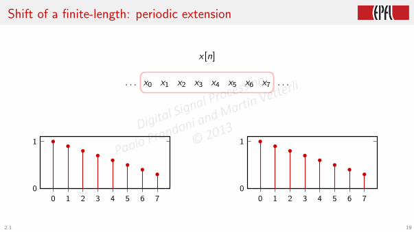
Shift of a finite-length: periodic extension
x [n]
. . . x0 x1 x2 x3 x4 x5 x6 x7 . . .
bb
bb
bb
bb
0 1 2 3 4 5 6 70
1 bb
bb
bb
bb
0 1 2 3 4 5 6 70
1
2.1 19
Digital Signal Processing
Paolo Prandoni and Martin Vetterli
© 2013

Shift of a finite-length: periodic extension
x̃ [n]
. . . x5 x6 x7 x0 x1 x2 x3 x4 x5 x6 x7 x0 x1 x2 . . .
bb
bb
bb
bb
0 1 2 3 4 5 6 70
1 bb
bb
bb
bb
0 1 2 3 4 5 6 70
1
2.1 19
Digital Signal Processing
Paolo Prandoni and Martin Vetterli
© 2013

Shift of a finite-length: periodic extension
x̃ [n − 1]
. . . x4 x5 x6 x7 x0 x1 x2 x3 x4 x5 x6 x7 x0 x1 . . .
bb
bb
bb
bb
0 1 2 3 4 5 6 70
1
b
bb
bb
bb
b
0 1 2 3 4 5 6 70
1
2.1 19
Digital Signal Processing
Paolo Prandoni and Martin Vetterli
© 2013

Shift of a finite-length: periodic extension
x̃ [n − 2]
. . . x3 x4 x5 x6 x7 x0 x1 x2 x3 x4 x5 x6 x7 x0 . . .
bb
bb
bb
bb
0 1 2 3 4 5 6 70
1
bb
bb
bb
bb
0 1 2 3 4 5 6 70
1
2.1 19
Digital Signal Processing
Paolo Prandoni and Martin Vetterli
© 2013
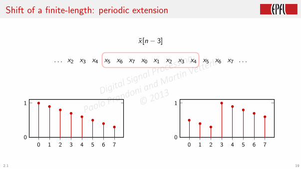
Shift of a finite-length: periodic extension
x̃ [n − 3]
. . . x2 x3 x4 x5 x6 x7 x0 x1 x2 x3 x4 x5 x6 x7 . . .
bb
bb
bb
bb
0 1 2 3 4 5 6 70
1
bb
b
bb
bb
b
0 1 2 3 4 5 6 70
1
2.1 19
Digital Signal Processing
Paolo Prandoni and Martin Vetterli
© 2013

Shift of a finite-length: periodic extension
x̃ [n − 4]
. . . x1 x2 x3 x4 x5 x6 x7 x0 x1 x2 x3 x4 x5 x6 . . .
bb
bb
bb
bb
0 1 2 3 4 5 6 70
1
bb
bb
bb
bb
0 1 2 3 4 5 6 70
1
2.1 19
Digital Signal Processing
Paolo Prandoni and Martin Vetterli
© 2013

Energy and power
Ex =∞∑
n=−∞
|x [n]|2
Px = limN→∞
1
2N + 1
N∑
n=−N
|x [n]|2
2.1 20
Digital Signal Processing
Paolo Prandoni and Martin Vetterli
© 2013

Energy and power
Ex =∞∑
n=−∞
|x [n]|2
Px = limN→∞
1
2N + 1
N∑
n=−N
|x [n]|2
2.1 20
Digital Signal Processing
Paolo Prandoni and Martin Vetterli
© 2013

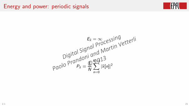
Energy and power: periodic signals
Ex̃ = ∞
Px̃ ≡1
N
N−1∑
n=0
|x̃ [n]|2
2.1 21
Digital Signal Processing
Paolo Prandoni and Martin Vetterli
© 2013
Energy and power: periodic signals
Ex̃ = ∞
Px̃ ≡1
N
N−1∑
n=0
|x̃ [n]|2
2.1 21
Digital Signal Processing
Paolo Prandoni and Martin Vetterli
© 2013

END OF MODULE 2.1
Digital Signal Processing
Paolo Prandoni and Martin Vetterli
© 2013
Digital Signal Processing
Module 2.2: the complex exponentialDigital Signal Processing
Paolo Prandoni and Martin Vetterli
© 2013

Overview:
◮ the complex exponential
◮ periodicity
◮ wagonwheel effect and maximum “speed”
◮ digital and real-world frequency
2.2 22
Digital Signal Processing
Paolo Prandoni and Martin Vetterli
© 2013

The complex exponential
The most important discrete-time signal in the world:
x [n] = e j(ωn+φ)
2.2 23
Digital Signal Processing
Paolo Prandoni and Martin Vetterli
© 2013

The complex exponential
Recall: e jα = cosα+ j sinα
−1 1
−1
1
Re
Im
ejα
b
α
2.2 24
Digital Signal Processing
Paolo Prandoni and Martin Vetterli
© 2013

The complex exponential
Rotation factor: z′ = z e jα
Re
Im
zb
2.2 25
Digital Signal Processing
Paolo Prandoni and Martin Vetterli
© 2013

The complex exponential
Rotation factor: z′ = z e jα
Re
Im
zb
z′b
α
2.2 25
Digital Signal Processing
Paolo Prandoni and Martin Vetterli
© 2013

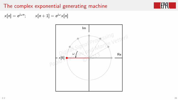
The complex exponential generating machine
x [n] = e jωn; x [n + 1] = e jωx [n]
Re
Im
x[0]b
2.2 26
Digital Signal Processing
Paolo Prandoni and Martin Vetterli
© 2013
The complex exponential generating machine
x [n] = e jωn; x [n + 1] = e jωx [n]
Re
Im
b
x[1]b
ω
2.2 26
Digital Signal Processing
Paolo Prandoni and Martin Vetterli
© 2013

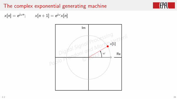
The complex exponential generating machine
x [n] = e jωn; x [n + 1] = e jωx [n]
Re
Im
b
b
x[2]b
ω
2.2 26
Digital Signal Processing
Paolo Prandoni and Martin Vetterli
© 2013

The complex exponential generating machine
x [n] = e jωn; x [n + 1] = e jωx [n]
Re
Im
b
b
b
x[3]b
ω
2.2 26
Digital Signal Processing
Paolo Prandoni and Martin Vetterli
© 2013

The complex exponential generating machine
x [n] = e jωn; x [n + 1] = e jωx [n]
Re
Im
b
b
bbx[4]
bω
2.2 26
Digital Signal Processing
Paolo Prandoni and Martin Vetterli
© 2013

The complex exponential generating machine
x [n] = e jωn; x [n + 1] = e jωx [n]
Re
Im
b
b
bb
b
x[5] b ω
2.2 26
Digital Signal Processing
Paolo Prandoni and Martin Vetterli
© 2013
The complex exponential generating machine
x [n] = e jωn; x [n + 1] = e jωx [n]
Re
Im
b
b
bb
b
b
x[6] bω
2.2 26
Digital Signal Processing
Paolo Prandoni and Martin Vetterli
© 2013

The complex exponential generating machine
x [n] = e jωn; x [n + 1] = e jωx [n]
Re
Im
b
b
bb
b
b
b
x[7]b
ω
2.2 26
Digital Signal Processing
Paolo Prandoni and Martin Vetterli
© 2013
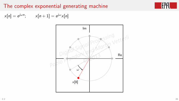
The complex exponential generating machine
x [n] = e jωn; x [n + 1] = e jωx [n]
Re
Im
b
b
bb
b
b
b
b
x[8]
b
ω
2.2 26
Digital Signal Processing
Paolo Prandoni and Martin Vetterli
© 2013
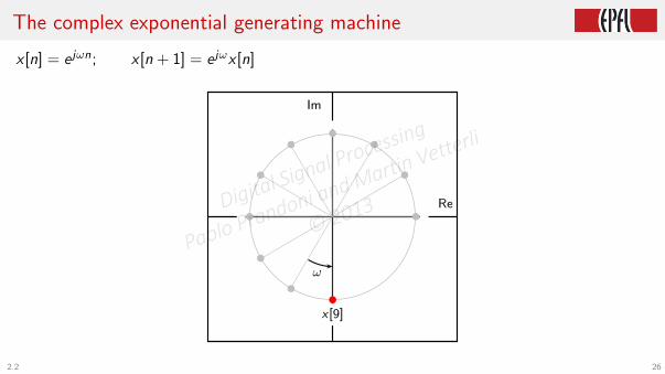
The complex exponential generating machine
x [n] = e jωn; x [n + 1] = e jωx [n]
Re
Im
b
b
bb
b
b
b
b
b
x[9]
b
ω
2.2 26
Digital Signal Processing
Paolo Prandoni and Martin Vetterli
© 2013

The complex exponential generating machine
x [n] = e jωn; x [n + 1] = e jωx [n]
Re
Im
b
b
bb
b
b
b
b
bb
x[10]
bω
2.2 26
Digital Signal Processing
Paolo Prandoni and Martin Vetterli
© 2013

The complex exponential generating machine
x [n] = e jωn; x [n + 1] = e jωx [n]
Re
Im
b
b
bb
b
b
b
b
bb
b
x[11]bω
2.2 26
Digital Signal Processing
Paolo Prandoni and Martin Vetterli
© 2013

The complex exponential generating machine
x [n] = e jωn; x [n + 1] = e jωx [n]
Re
Im
b
b
bb
b
b
b
b
bb
b
b
x[12]bω
2.2 26
Digital Signal Processing
Paolo Prandoni and Martin Vetterli
© 2013

The complex exponential generating machine
x [n] = e jωn; x [n + 1] = e jωx [n]
Re
Im
b
b
bb
b
b
b
b
bb
b
b
b
x[13]b
ω
2.2 26
Digital Signal Processing
Paolo Prandoni and Martin Vetterli
© 2013

The complex exponential generating machine
x [n] = e jωn; x [n + 1] = e jωx [n]
Re
Im
b
b
bb
b
b
b
b
bb
b
b
b
b
x[14]b
ω
2.2 26
Digital Signal Processing
Paolo Prandoni and Martin Vetterli
© 2013

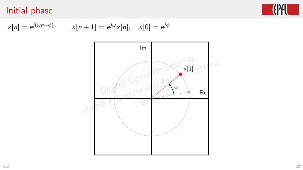
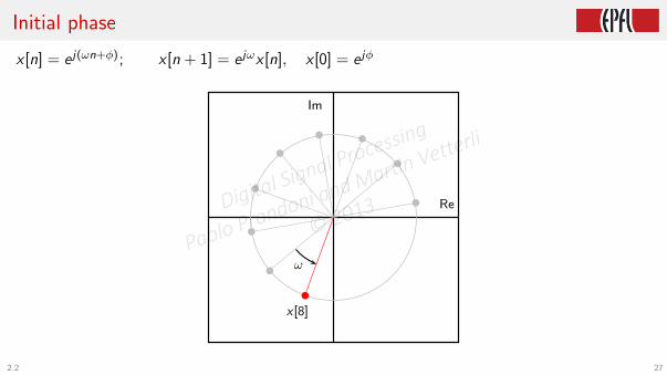
Initial phase
x [n] = e j(ωn+φ); x [n + 1] = e jωx [n], x [0] = e jφ
Re
Im
x[0]b
2.2 27
Digital Signal Processing
Paolo Prandoni and Martin Vetterli
© 2013
Initial phase
x [n] = e j(ωn+φ); x [n + 1] = e jωx [n], x [0] = e jφ
Re
Im
b
x[1]b
ω
2.2 27
Digital Signal Processing
Paolo Prandoni and Martin Vetterli
© 2013

Initial phase
x [n] = e j(ωn+φ); x [n + 1] = e jωx [n], x [0] = e jφ
Re
Im
b
b
x[2]b
ω
2.2 27
Digital Signal Processing
Paolo Prandoni and Martin Vetterli
© 2013

Initial phase
x [n] = e j(ωn+φ); x [n + 1] = e jωx [n], x [0] = e jφ
Re
Im
b
b
bx[3]
b
ω
2.2 27
Digital Signal Processing
Paolo Prandoni and Martin Vetterli
© 2013

Initial phase
x [n] = e j(ωn+φ); x [n + 1] = e jωx [n], x [0] = e jφ
Re
Im
b
b
bbx[4]
bω
2.2 27
Digital Signal Processing
Paolo Prandoni and Martin Vetterli
© 2013

Initial phase
x [n] = e j(ωn+φ); x [n + 1] = e jωx [n], x [0] = e jφ
Re
Im
b
b
bbb
x[5] b ω
2.2 27
Digital Signal Processing
Paolo Prandoni and Martin Vetterli
© 2013

Initial phase
x [n] = e j(ωn+φ); x [n + 1] = e jωx [n], x [0] = e jφ
Re
Im
b
b
bbb
b
x[6] bω
2.2 27
Digital Signal Processing
Paolo Prandoni and Martin Vetterli
© 2013

Initial phase
x [n] = e j(ωn+φ); x [n + 1] = e jωx [n], x [0] = e jφ
Re
Im
b
b
bbb
b
b
x[7]b
ω
2.2 27
Digital Signal Processing
Paolo Prandoni and Martin Vetterli
© 2013
Initial phase
x [n] = e j(ωn+φ); x [n + 1] = e jωx [n], x [0] = e jφ
Re
Im
b
b
bbb
b
b
b
x[8]
b
ω
2.2 27
Digital Signal Processing
Paolo Prandoni and Martin Vetterli
© 2013

Initial phase
x [n] = e j(ωn+φ); x [n + 1] = e jωx [n], x [0] = e jφ
Re
Im
b
b
bbb
b
b
b
b
x[9]
b
ω
2.2 27
Digital Signal Processing
Paolo Prandoni and Martin Vetterli
© 2013

Initial phase
x [n] = e j(ωn+φ); x [n + 1] = e jωx [n], x [0] = e jφ
Re
Im
b
b
bbb
b
b
b
b b x[10]
bω
2.2 27
Digital Signal Processing
Paolo Prandoni and Martin Vetterli
© 2013

Initial phase
x [n] = e j(ωn+φ); x [n + 1] = e jωx [n], x [0] = e jφ
Re
Im
b
b
bbb
b
b
b
b bb
x[11]b
ω
2.2 27
Digital Signal Processing
Paolo Prandoni and Martin Vetterli
© 2013

Initial phase
x [n] = e j(ωn+φ); x [n + 1] = e jωx [n], x [0] = e jφ
Re
Im
b
b
bbb
b
b
b
b bb
b
x[12]b
ω
2.2 27
Digital Signal Processing
Paolo Prandoni and Martin Vetterli
© 2013

Initial phase
x [n] = e j(ωn+φ); x [n + 1] = e jωx [n], x [0] = e jφ
Re
Im
b
b
bbb
b
b
b
b bb
b
b
x[13]b
ω
2.2 27
Digital Signal Processing
Paolo Prandoni and Martin Vetterli
© 2013

Initial phase
x [n] = e j(ωn+φ); x [n + 1] = e jωx [n], x [0] = e jφ
Re
Im
b
b
bbb
b
b
b
b bb
b
b
b
x[14]b
ω
2.2 27
Digital Signal Processing
Paolo Prandoni and Martin Vetterli
© 2013
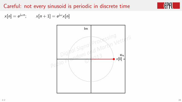
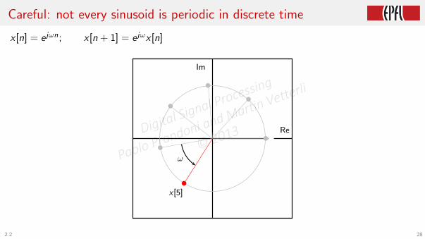
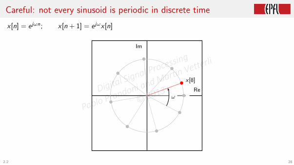
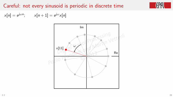
Careful: not every sinusoid is periodic in discrete time
x [n] = e jωn; x [n + 1] = e jωx [n]
Re
Im
x[0]b
2.2 28
Digital Signal Processing
Paolo Prandoni and Martin Vetterli
© 2013

Careful: not every sinusoid is periodic in discrete time
x [n] = e jωn; x [n + 1] = e jωx [n]
Re
Im
b
x[1]b
ω
2.2 28
Digital Signal Processing
Paolo Prandoni and Martin Vetterli
© 2013

Careful: not every sinusoid is periodic in discrete time
x [n] = e jωn; x [n + 1] = e jωx [n]
Re
Im
b
b
x[2]b
ω
2.2 28
Digital Signal Processing
Paolo Prandoni and Martin Vetterli
© 2013

Careful: not every sinusoid is periodic in discrete time
x [n] = e jωn; x [n + 1] = e jωx [n]
Re
Im
b
b
b
x[3]b ω
2.2 28
Digital Signal Processing
Paolo Prandoni and Martin Vetterli
© 2013

Careful: not every sinusoid is periodic in discrete time
x [n] = e jωn; x [n + 1] = e jωx [n]
Re
Im
b
b
b
b
x[4] b
ω
2.2 28
Digital Signal Processing
Paolo Prandoni and Martin Vetterli
© 2013
Careful: not every sinusoid is periodic in discrete time
x [n] = e jωn; x [n + 1] = e jωx [n]
Re
Im
b
b
b
b
b
x[5]
b
ω
2.2 28
Digital Signal Processing
Paolo Prandoni and Martin Vetterli
© 2013

Careful: not every sinusoid is periodic in discrete time
x [n] = e jωn; x [n + 1] = e jωx [n]
Re
Im
b
b
b
b
b
b
x[6]
b
ω
2.2 28
Digital Signal Processing
Paolo Prandoni and Martin Vetterli
© 2013

Careful: not every sinusoid is periodic in discrete time
x [n] = e jωn; x [n + 1] = e jωx [n]
Re
Im
b
b
b
b
b
bb
x[7]b
ω
2.2 28
Digital Signal Processing
Paolo Prandoni and Martin Vetterli
© 2013
Careful: not every sinusoid is periodic in discrete time
x [n] = e jωn; x [n + 1] = e jωx [n]
Re
Im
b
b
b
b
b
bb
b
x[8]b
ω
2.2 28
Digital Signal Processing
Paolo Prandoni and Martin Vetterli
© 2013

Careful: not every sinusoid is periodic in discrete time
x [n] = e jωn; x [n + 1] = e jωx [n]
Re
Im
b
b
b
b
b
bb
b
b
x[9]b
ω
2.2 28
Digital Signal Processing
Paolo Prandoni and Martin Vetterli
© 2013

Careful: not every sinusoid is periodic in discrete time
x [n] = e jωn; x [n + 1] = e jωx [n]
Re
Im
b
b
b
b
b
bb
b
b
bx[10]
b
ω
2.2 28
Digital Signal Processing
Paolo Prandoni and Martin Vetterli
© 2013
Careful: not every sinusoid is periodic in discrete time
x [n] = e jωn; x [n + 1] = e jωx [n]
Re
Im
b
b
b
b
b
bb
b
b
bb
x[11] bω
2.2 28
Digital Signal Processing
Paolo Prandoni and Martin Vetterli
© 2013

Careful: not every sinusoid is periodic in discrete time
x [n] = e jωn; x [n + 1] = e jωx [n]
Re
Im
b
b
b
b
b
bb
b
b
bb
b
x[12]b
ω
2.2 28
Digital Signal Processing
Paolo Prandoni and Martin Vetterli
© 2013

Careful: not every sinusoid is periodic in discrete time
x [n] = e jωn; x [n + 1] = e jωx [n]
Re
Im
b
b
b
b
b
bb
b
b
bb
b
b
x[13]
b
ω
2.2 28
Digital Signal Processing
Paolo Prandoni and Martin Vetterli
© 2013

Careful: not every sinusoid is periodic in discrete time
x [n] = e jωn; x [n + 1] = e jωx [n]
Re
Im
b
b
b
b
b
bb
b
b
bb
b
b
bx[14]
bω
2.2 28
Digital Signal Processing
Paolo Prandoni and Martin Vetterli
© 2013

Periodicity
e jωn periodic ⇐⇒ ω =M
N2π,M,N ∈ N
e jω = e j(ω+2kπ) ∀k ∈ N
2.2 29
Digital Signal Processing
Paolo Prandoni and Martin Vetterli
© 2013

Periodicity
e jωn periodic ⇐⇒ ω =M
N2π,M,N ∈ N
e jω = e j(ω+2kπ) ∀k ∈ N
2.2 29
Digital Signal Processing
Paolo Prandoni and Martin Vetterli
© 2013

Quiz
◮ is the signal e jn periodic?
2.2 30
Digital Signal Processing
Paolo Prandoni and Martin Vetterli
© 2013

One point, many names
Re
Im
ejα
b
α
2.2 31
Digital Signal Processing
Paolo Prandoni and Martin Vetterli
© 2013

One point, many names
Re
Im
ejα
b
2π + α
2.2 31
Digital Signal Processing
Paolo Prandoni and Martin Vetterli
© 2013

One point, many names
Re
Im
ejα
b
6π + α
2.2 31
Digital Signal Processing
Paolo Prandoni and Martin Vetterli
© 2013

One point, many names
Re
Im
ejα
b
α
2.2 32
Digital Signal Processing
Paolo Prandoni and Martin Vetterli
© 2013

One point, many names
Re
Im
ejα
b
α
−2π + α
2.2 32
Digital Signal Processing
Paolo Prandoni and Martin Vetterli
© 2013

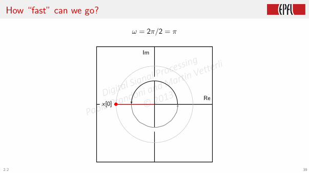
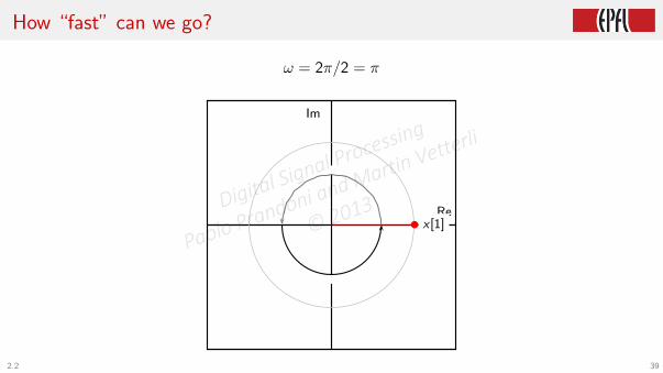
How “fast” can we go?
2.2 33
Digital Signal Processing
Paolo Prandoni and Martin Vetterli
© 2013
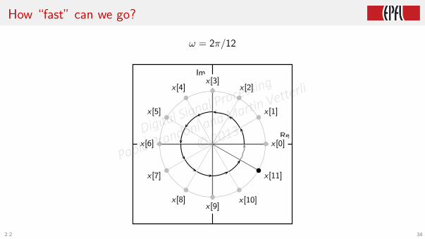
How “fast” can we go?
ω = 2π/12
Re
Im
x[0]b
x[1]b
x[2]b
x[3]bx[4]
b
x[5] b
x[6] b
x[7]b
x[8]
b
x[9]
bx[10]
b
x[11]b
2.2 34
Digital Signal Processing
Paolo Prandoni and Martin Vetterli
© 2013

How “fast” can we go?
ω = 2π/6
Re
Im
x[0]b
x[1]b
x[2]b
x[3] b
x[4]
b
x[5]
b
2.2 35
Digital Signal Processing
Paolo Prandoni and Martin Vetterli
© 2013

How “fast” can we go?
ω = 2π/5
Re
Im
x[0]b
x[1]b
x[2] b
x[3]b
x[4]
b
2.2 36
Digital Signal Processing
Paolo Prandoni and Martin Vetterli
© 2013
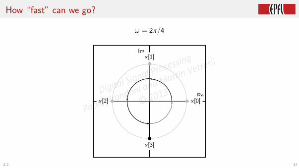
How “fast” can we go?
ω = 2π/4
Re
Im
x[0]b
x[1]b
x[2] b
x[3]
b
2.2 37
Digital Signal Processing
Paolo Prandoni and Martin Vetterli
© 2013

How “fast” can we go?
ω = 2π/3
Re
Im
x[0]b
x[1]b
x[2]
b
2.2 38
Digital Signal Processing
Paolo Prandoni and Martin Vetterli
© 2013
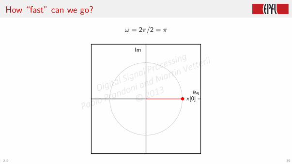
How “fast” can we go?
ω = 2π/2 = π
Re
Im
x[0]b
2.2 39
Digital Signal Processing
Paolo Prandoni and Martin Vetterli
© 2013
How “fast” can we go?
ω = 2π/2 = π
Re
Im
x[0] b
2.2 39
Digital Signal Processing
Paolo Prandoni and Martin Vetterli
© 2013
How “fast” can we go?
ω = 2π/2 = π
Re
Im
x[1]b
2.2 39
Digital Signal Processing
Paolo Prandoni and Martin Vetterli
© 2013

How “fast” can we go?
ω = 2π/2 = π
Re
Im
x[2] b
2.2 39
Digital Signal Processing
Paolo Prandoni and Martin Vetterli
© 2013

How “fast” can we go?
ω = 2π/2 = π
Re
Im
x[3]b
2.2 39
Digital Signal Processing
Paolo Prandoni and Martin Vetterli
© 2013

How “fast” can we go?
ω = 2π/2 = π
Re
Im
x[4] b
2.2 39
Digital Signal Processing
Paolo Prandoni and Martin Vetterli
© 2013

How “fast” can we go?
ω = 2π/2 = π
Re
Im
x[5]b
2.2 39
Digital Signal Processing
Paolo Prandoni and Martin Vetterli
© 2013
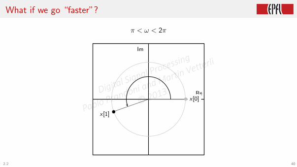
What if we go “faster”?
π < ω < 2π
Re
Im
x[0]b
x[1]b
2.2 40
Digital Signal Processing
Paolo Prandoni and Martin Vetterli
© 2013

What if we go “faster”?
π < ω < 2π
Re
Im
x[0]b
x[1]b
ω − 2π
2.2 40
Digital Signal Processing
Paolo Prandoni and Martin Vetterli
© 2013

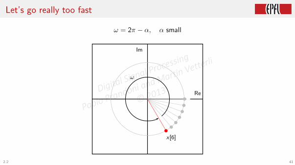
Let’s go really too fast
ω = 2π − α, α small
Re
Im
x[0]b
2.2 41
Digital Signal Processing
Paolo Prandoni and Martin Vetterli
© 2013

Let’s go really too fast
ω = 2π − α, α small
Re
Im
b
x[1]bω
2.2 41
Digital Signal Processing
Paolo Prandoni and Martin Vetterli
© 2013

Let’s go really too fast
ω = 2π − α, α small
Re
Im
bb
x[2]b
ω
2.2 41
Digital Signal Processing
Paolo Prandoni and Martin Vetterli
© 2013
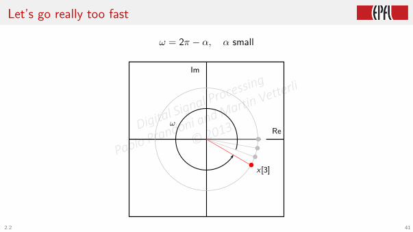
Let’s go really too fast
ω = 2π − α, α small
Re
Im
bbb
x[3]b
ω
2.2 41
Digital Signal Processing
Paolo Prandoni and Martin Vetterli
© 2013

Let’s go really too fast
ω = 2π − α, α small
Re
Im
bbbb
x[4]b
ω
2.2 41
Digital Signal Processing
Paolo Prandoni and Martin Vetterli
© 2013

Let’s go really too fast
ω = 2π − α, α small
Re
Im
bbbb
b
x[5]
b
ω
2.2 41
Digital Signal Processing
Paolo Prandoni and Martin Vetterli
© 2013
Let’s go really too fast
ω = 2π − α, α small
Re
Im
bbbb
bb
x[6]
b
ω
2.2 41
Digital Signal Processing
Paolo Prandoni and Martin Vetterli
© 2013

Let’s go really too fast
ω = 2π − α, α small
Re
Im
bbbb
bb
b
x[7]
b
ω
2.2 41
Digital Signal Processing
Paolo Prandoni and Martin Vetterli
© 2013

The wagonwheel effect
2.2 42
Digital Signal Processing
Paolo Prandoni and Martin Vetterli
© 2013

Digital vs physical frequency
◮ Discrete time:
• n: no physical dimension (just a counter)
• periodicity: how many samples before pattern repeats
◮ “Real world”:
• periodicity: how many seconds before pattern repeats
• frequency measured in Hz (s−1)
2.2 43
Digital Signal Processing
Paolo Prandoni and Martin Vetterli
© 2013

How your PC plays sounds
x [n] sound card
2.2 44
Digital Signal Processing
Paolo Prandoni and Martin Vetterli
© 2013

How your PC plays sounds
x [n] sound card
Ts system clock
2.2 44
Digital Signal Processing
Paolo Prandoni and Martin Vetterli
© 2013

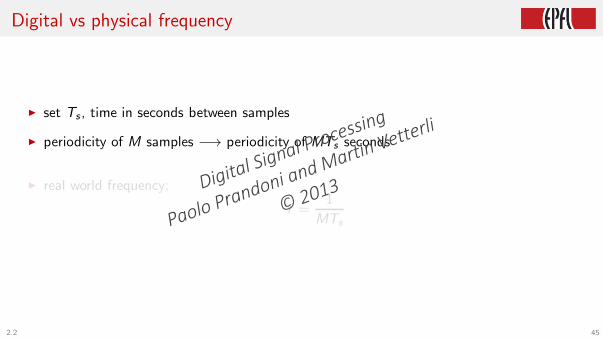
Digital vs physical frequency
◮ set Ts , time in seconds between samples
◮ periodicity of M samples −→ periodicity of MTs seconds
◮ real world frequency:
f =1
MTs
2.2 45
Digital Signal Processing
Paolo Prandoni and Martin Vetterli
© 2013
Digital vs physical frequency
◮ set Ts , time in seconds between samples
◮ periodicity of M samples −→ periodicity of MTs seconds
◮ real world frequency:
f =1
MTs
2.2 45
Digital Signal Processing
Paolo Prandoni and Martin Vetterli
© 2013

Digital vs physical frequency
◮ set Ts , time in seconds between samples
◮ periodicity of M samples −→ periodicity of MTs seconds
◮ real world frequency:
f =1
MTs
2.2 45
Digital Signal Processing
Paolo Prandoni and Martin Vetterli
© 2013

END OF MODULE 2.2
Digital Signal Processing
Paolo Prandoni and Martin Vetterli
© 2013

Digital Signal Processing
Module 2.3: the Karplus-Strong algorithmDigital Signal Processing
Paolo Prandoni and Martin Vetterli
© 2013

Overview:
◮ DSP building blocks
◮ moving averages and simple feedback loops
◮ a sound synthesizer
2.3 46
Digital Signal Processing
Paolo Prandoni and Martin Vetterli
© 2013

Overview:
◮ DSP as Lego: The fundamental building blocks
◮ Averages and moving averages
◮ Recursion: Revisiting your bank account
◮ Building a simple recursive synthesizer
◮ Examples of sounds
2.3 47
Digital Signal Processing
Paolo Prandoni and Martin Vetterli
© 2013

DSP as Lego
x [n] b + b + y [n]
z−1
+ b z−3
z−1
a b
−1
c
2.3 48
Digital Signal Processing
Paolo Prandoni and Martin Vetterli
© 2013

Building Blocks: Adder
x [n]
+ x [n] + y [n]
y [n]
2.3 49
Digital Signal Processing
Paolo Prandoni and Martin Vetterli
© 2013

Building Blocks: Adder
x [n]
+ x [n] + y [n]
y [n]
b b b b b b b b b b b
0 2 4 6 8 100
1
b b b b b b b b b b b
0 2 4 6 8 100
1
2.3 49
Digital Signal Processing
Paolo Prandoni and Martin Vetterli
© 2013

Building Blocks: Adder
x [n]
+ x [n] + y [n]
y [n]
b b b b b b b b b b b
0 2 4 6 8 100
1
b b b b b b b b b b b
0 2 4 6 8 100
1
b b b b b b b b b b b
0 2 4 6 8 100
1
2.3 49
Digital Signal Processing
Paolo Prandoni and Martin Vetterli
© 2013

Building Blocks: Multiplier
x [n] αx [n]α
2.3 50
Digital Signal Processing
Paolo Prandoni and Martin Vetterli
© 2013

Building Blocks: Multiplier
x [n] αx [n]α
bb
bb
bb
bb
bb
b
0 2 4 6 8 100
1
2.3 50
Digital Signal Processing
Paolo Prandoni and Martin Vetterli
© 2013

Building Blocks: Multiplier
x [n] αx [n]α
bb
bb
bb
bb
bb
b
0 2 4 6 8 100
1
b b b b b b b b b b b
0 2 4 6 8 100
1
α = 0.5
2.3 50
Digital Signal Processing
Paolo Prandoni and Martin Vetterli
© 2013
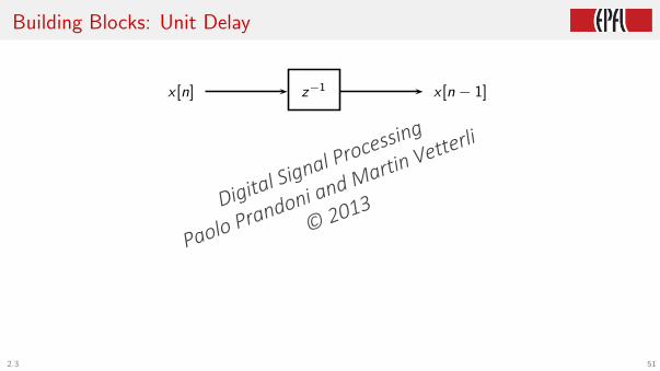
Building Blocks: Unit Delay
x [n] z−1 x [n − 1]
2.3 51
Digital Signal Processing
Paolo Prandoni and Martin Vetterli
© 2013

Building Blocks: Unit Delay
x [n] z−1 x [n − 1]
bb
bb
bb
bb
bb
b
0 2 4 6 8 100
1
2.3 51
Digital Signal Processing
Paolo Prandoni and Martin Vetterli
© 2013

Building Blocks: Unit Delay
x [n] z−1 x [n − 1]
bb
bb
bb
bb
bb
b
0 2 4 6 8 100
1
bb
bb
bb
bb
bb
bb
0 2 4 6 8 100
1
2.3 51
Digital Signal Processing
Paolo Prandoni and Martin Vetterli
© 2013

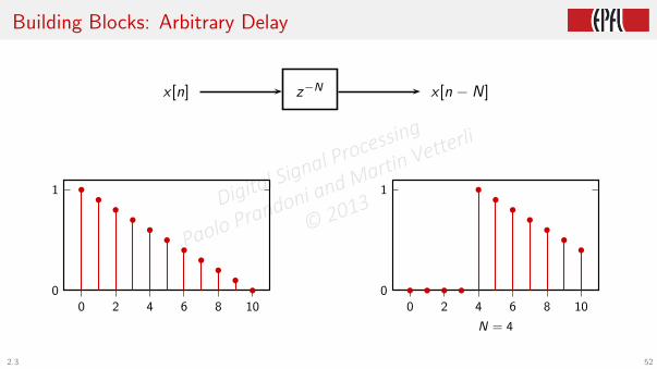
Building Blocks: Arbitrary Delay
x [n] z−N x [n − N]
2.3 52
Digital Signal Processing
Paolo Prandoni and Martin Vetterli
© 2013

Building Blocks: Arbitrary Delay
x [n] z−N x [n − N]
bb
bb
bb
bb
bb
b
0 2 4 6 8 100
1
2.3 52
Digital Signal Processing
Paolo Prandoni and Martin Vetterli
© 2013
Building Blocks: Arbitrary Delay
x [n] z−N x [n − N]
bb
bb
bb
bb
bb
b
0 2 4 6 8 100
1
b b b b
bb
bb
bb
b
0 2 4 6 8 100
1
N = 4
2.3 52
Digital Signal Processing
Paolo Prandoni and Martin Vetterli
© 2013

The 2-point Moving Average
◮ simple average:
m =a + b
2
◮ moving average: take a “local” average
y [n] =x [n] + x [n − 1]
2
2.3 53
Digital Signal Processing
Paolo Prandoni and Martin Vetterli
© 2013

The 2-point Moving Average
◮ simple average:
m =a + b
2
◮ moving average: take a “local” average
y [n] =x [n] + x [n − 1]
2
2.3 53
Digital Signal Processing
Paolo Prandoni and Martin Vetterli
© 2013

The 2-point Moving Average Using Lego
x [n] b + y [n]
z−1
1/2
2.3 54
Digital Signal Processing
Paolo Prandoni and Martin Vetterli
© 2013

Let’s average...
x [n] = δ[n]
b b
b
b b b b b b b b b b
−2 0 2 4 6 8 10
−1
0
1
2.3 55
Digital Signal Processing
Paolo Prandoni and Martin Vetterli
© 2013

Let’s average...
x [n] = δ[n]
b b
b
b b b b b b b b b b
−2 0 2 4 6 8 10
−1
0
1
b b
b b
b b b b b b b b b
−2 0 2 4 6 8 10
−1
0
1
2.3 55
Digital Signal Processing
Paolo Prandoni and Martin Vetterli
© 2013

Let’s average...
x [n] = u[n]
b b
b b b b b b b b b b b
−2 0 2 4 6 8 10
−1
0
1
2.3 56
Digital Signal Processing
Paolo Prandoni and Martin Vetterli
© 2013

Let’s average...
x [n] = u[n]
b b
b b b b b b b b b b b
−2 0 2 4 6 8 10
−1
0
1
b b
b
b b b b b b b b b b
−2 0 2 4 6 8 10
−1
0
1
2.3 56
Digital Signal Processing
Paolo Prandoni and Martin Vetterli
© 2013

Let’s average...
x [n] = cos(ωn), ω = π/10
bb b b
b
b
b
b
b
b
bb b
−2 0 2 4 6 8 10
−1
0
1
2.3 57
Digital Signal Processing
Paolo Prandoni and Martin Vetterli
© 2013

Let’s average...
x [n] = cos(ωn), ω = π/10
bb b b
b
b
b
b
b
b
bb b
−2 0 2 4 6 8 10
−1
0
1b
bb b
bb
b
b
b
b
bb
b
−2 0 2 4 6 8 10
−1
0
1
2.3 57
Digital Signal Processing
Paolo Prandoni and Martin Vetterli
© 2013

Let’s average...
x [n] = cos(ωn), ω = π
b
b
b
b
b
b
b
b
b
b
b
b
b
−2 0 2 4 6 8 10
−1
0
1
2.3 58
Digital Signal Processing
Paolo Prandoni and Martin Vetterli
© 2013
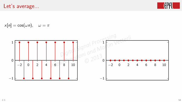
Let’s average...
x [n] = cos(ωn), ω = π
b
b
b
b
b
b
b
b
b
b
b
b
b
−2 0 2 4 6 8 10
−1
0
1
b b b b b b b b b b b b b
−2 0 2 4 6 8 10
−1
0
1
2.3 58
Digital Signal Processing
Paolo Prandoni and Martin Vetterli
© 2013

What if we reverse the loop?
x [n] b + y [n]
z−1
1/2
2.3 59
Digital Signal Processing
Paolo Prandoni and Martin Vetterli
© 2013

What if we reverse the loop?
x [n] + b y [n]
z−1α
2.3 59
Digital Signal Processing
Paolo Prandoni and Martin Vetterli
© 2013

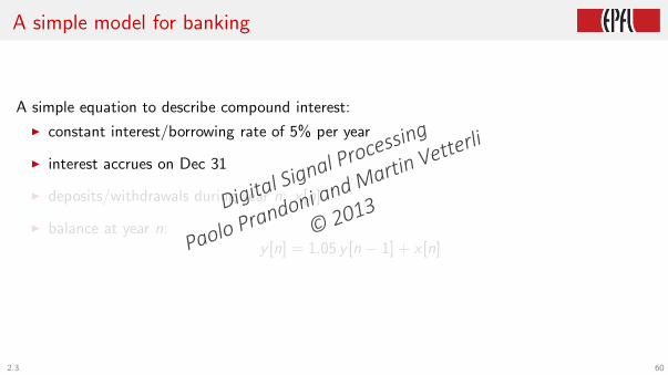
A simple model for banking
A simple equation to describe compound interest:
◮ constant interest/borrowing rate of 5% per year
◮ interest accrues on Dec 31
◮ deposits/withdrawals during year n: x [n]
◮ balance at year n:y [n] = 1.05 y [n − 1] + x [n]
2.3 60
Digital Signal Processing
Paolo Prandoni and Martin Vetterli
© 2013

First-order recursion
x [n] + b y [n]
z−11.05
y [n] = 1.05 y [n − 1] + x [n]
2.3 61
Digital Signal Processing
Paolo Prandoni and Martin Vetterli
© 2013

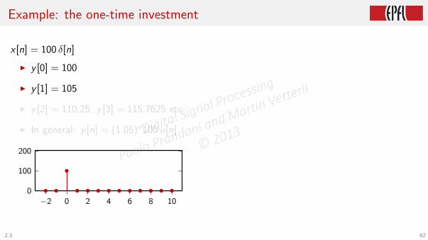
Example: the one-time investment
x [n] = 100 δ[n]
◮ y [0] = 100
◮ y [1] = 105
◮ y [2] = 110.25, y [3] = 115.7625 etc.
◮ In general: y [n] = (1.05)n100 u[n]
b b
b
b b b b b b b b b b
−2 0 2 4 6 8 100
100
200
2.3 62
Digital Signal Processing
Paolo Prandoni and Martin Vetterli
© 2013

Example: the one-time investment
x [n] = 100 δ[n]
◮ y [0] = 100
◮ y [1] = 105
◮ y [2] = 110.25, y [3] = 115.7625 etc.
◮ In general: y [n] = (1.05)n100 u[n]
b b
b
b b b b b b b b b b
−2 0 2 4 6 8 100
100
200
2.3 62
Digital Signal Processing
Paolo Prandoni and Martin Vetterli
© 2013
Example: the one-time investment
x [n] = 100 δ[n]
◮ y [0] = 100
◮ y [1] = 105
◮ y [2] = 110.25, y [3] = 115.7625 etc.
◮ In general: y [n] = (1.05)n100 u[n]
b b
b
b b b b b b b b b b
−2 0 2 4 6 8 100
100
200
2.3 62
Digital Signal Processing
Paolo Prandoni and Martin Vetterli
© 2013

Example: the one-time investment
x [n] = 100 δ[n]
◮ y [0] = 100
◮ y [1] = 105
◮ y [2] = 110.25, y [3] = 115.7625 etc.
◮ In general: y [n] = (1.05)n100 u[n]
b b
b
b b b b b b b b b b
−2 0 2 4 6 8 100
100
200
2.3 62
Digital Signal Processing
Paolo Prandoni and Martin Vetterli
© 2013

Example: the one-time investment
x [n] = 100 δ[n]
◮ y [0] = 100
◮ y [1] = 105
◮ y [2] = 110.25, y [3] = 115.7625 etc.
◮ In general: y [n] = (1.05)n100 u[n]
b b
b
b b b b b b b b b b
−2 0 2 4 6 8 100
100
200
b b
b b b b b b b b b b b
−2 0 2 4 6 8 100
100
200
2.3 62
Digital Signal Processing
Paolo Prandoni and Martin Vetterli
© 2013

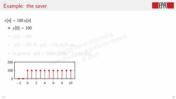
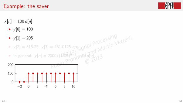
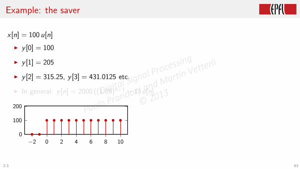
Example: the saver
x [n] = 100 u[n]
◮ y [0] = 100
◮ y [1] = 205
◮ y [2] = 315.25, y [3] = 431.0125 etc.
◮ In general: y [n] = 2000 ((1.05)n+1 − 1) u[n]
b b
b b b b b b b b b b b
−2 0 2 4 6 8 100
100
200
2.3 63
Digital Signal Processing
Paolo Prandoni and Martin Vetterli
© 2013
Example: the saver
x [n] = 100 u[n]
◮ y [0] = 100
◮ y [1] = 205
◮ y [2] = 315.25, y [3] = 431.0125 etc.
◮ In general: y [n] = 2000 ((1.05)n+1 − 1) u[n]
b b
b b b b b b b b b b b
−2 0 2 4 6 8 100
100
200
2.3 63
Digital Signal Processing
Paolo Prandoni and Martin Vetterli
© 2013
Example: the saver
x [n] = 100 u[n]
◮ y [0] = 100
◮ y [1] = 205
◮ y [2] = 315.25, y [3] = 431.0125 etc.
◮ In general: y [n] = 2000 ((1.05)n+1 − 1) u[n]
b b
b b b b b b b b b b b
−2 0 2 4 6 8 100
100
200
2.3 63
Digital Signal Processing
Paolo Prandoni and Martin Vetterli
© 2013
Example: the saver
x [n] = 100 u[n]
◮ y [0] = 100
◮ y [1] = 205
◮ y [2] = 315.25, y [3] = 431.0125 etc.
◮ In general: y [n] = 2000 ((1.05)n+1 − 1) u[n]
b b
b b b b b b b b b b b
−2 0 2 4 6 8 100
100
200
2.3 63
Digital Signal Processing
Paolo Prandoni and Martin Vetterli
© 2013

Example: the saver
x [n] = 100 u[n]
◮ y [0] = 100
◮ y [1] = 205
◮ y [2] = 315.25, y [3] = 431.0125 etc.
◮ In general: y [n] = 2000 ((1.05)n+1 − 1) u[n]
b b
b b b b b b b b b b b
−2 0 2 4 6 8 100
100
200
b b b b b b b b bb
bb
b
−2 0 2 4 6 8 100
500
1000
1500
2.3 63
Digital Signal Processing
Paolo Prandoni and Martin Vetterli
© 2013

Example: The independently wealthy
x [n] = 100 δ[n] − 5 u[n − 1]
◮ y [0] = 100
◮ y [1] = 100
◮ y [2] = 100, y [3] = 100 etc.
◮ In general: y [n] = 100 u[n]
b b
b
b b b b b b b b b b
−2 0 2 4 6 8 10
0
100
2.3 64
Digital Signal Processing
Paolo Prandoni and Martin Vetterli
© 2013

Example: The independently wealthy
x [n] = 100 δ[n] − 5 u[n − 1]
◮ y [0] = 100
◮ y [1] = 100
◮ y [2] = 100, y [3] = 100 etc.
◮ In general: y [n] = 100 u[n]
b b
b
b b b b b b b b b b
−2 0 2 4 6 8 10
0
100
2.3 64
Digital Signal Processing
Paolo Prandoni and Martin Vetterli
© 2013

Example: The independently wealthy
x [n] = 100 δ[n] − 5 u[n − 1]
◮ y [0] = 100
◮ y [1] = 100
◮ y [2] = 100, y [3] = 100 etc.
◮ In general: y [n] = 100 u[n]
b b
b
b b b b b b b b b b
−2 0 2 4 6 8 10
0
100
2.3 64
Digital Signal Processing
Paolo Prandoni and Martin Vetterli
© 2013

Example: The independently wealthy
x [n] = 100 δ[n] − 5 u[n − 1]
◮ y [0] = 100
◮ y [1] = 100
◮ y [2] = 100, y [3] = 100 etc.
◮ In general: y [n] = 100 u[n]
b b
b
b b b b b b b b b b
−2 0 2 4 6 8 10
0
100
2.3 64
Digital Signal Processing
Paolo Prandoni and Martin Vetterli
© 2013

Example: The independently wealthy
x [n] = 100 δ[n] − 5 u[n − 1]
◮ y [0] = 100
◮ y [1] = 100
◮ y [2] = 100, y [3] = 100 etc.
◮ In general: y [n] = 100 u[n]
b b
b
b b b b b b b b b b
−2 0 2 4 6 8 10
0
100
b b
b b b b b b b b b b b
−2 0 2 4 6 8 100
100
200
2.3 64
Digital Signal Processing
Paolo Prandoni and Martin Vetterli
© 2013
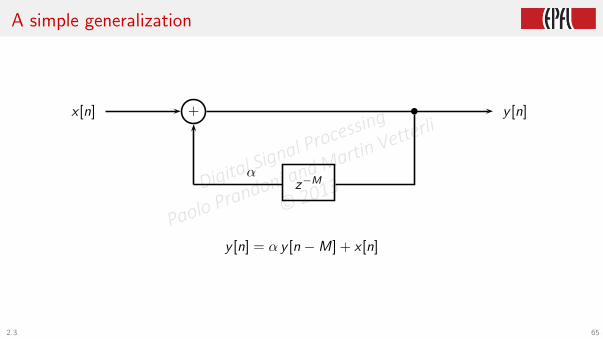
A simple generalization
x [n] + b y [n]
z−Mα
y [n] = α y [n −M] + x [n]
2.3 65
Digital Signal Processing
Paolo Prandoni and Martin Vetterli
© 2013

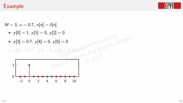
Example
M = 3, α = 0.7, x [n] = δ[n]
◮ y [0] = 1, y [1] = 0, y [2] = 0
◮ y [3] = 0.7, y [4] = 0, y [5] = 0
◮ y [6] = 0.72, y [7] = 0, y [8] = 0, etc.
b b
b
b b b b b b b b b b
−2 0 2 4 6 8 100
1
2.3 66
Digital Signal Processing
Paolo Prandoni and Martin Vetterli
© 2013

Example
M = 3, α = 0.7, x [n] = δ[n]
◮ y [0] = 1, y [1] = 0, y [2] = 0
◮ y [3] = 0.7, y [4] = 0, y [5] = 0
◮ y [6] = 0.72, y [7] = 0, y [8] = 0, etc.
b b
b
b b b b b b b b b b
−2 0 2 4 6 8 100
1
2.3 66
Digital Signal Processing
Paolo Prandoni and Martin Vetterli
© 2013
Example
M = 3, α = 0.7, x [n] = δ[n]
◮ y [0] = 1, y [1] = 0, y [2] = 0
◮ y [3] = 0.7, y [4] = 0, y [5] = 0
◮ y [6] = 0.72, y [7] = 0, y [8] = 0, etc.
b b
b
b b b b b b b b b b
−2 0 2 4 6 8 100
1
2.3 66
Digital Signal Processing
Paolo Prandoni and Martin Vetterli
© 2013

Example
M = 3, α = 0.7, x [n] = δ[n]
◮ y [0] = 1, y [1] = 0, y [2] = 0
◮ y [3] = 0.7, y [4] = 0, y [5] = 0
◮ y [6] = 0.72, y [7] = 0, y [8] = 0, etc.
b b
b
b b b b b b b b b b
−2 0 2 4 6 8 100
1
b b
b
b b
b
b b
b
b bb
b
−2 0 2 4 6 8 100
1
2.3 66
Digital Signal Processing
Paolo Prandoni and Martin Vetterli
© 2013

Example
M = 3, α = 1, x [n] = δ[n] + 2 δ[n − 1] + 3 δ[n − 2]
◮ y [0] = 1, y [1] = 2, y [2] = 3
◮ y [3] = 1, y [4] = 2, y [5] = 3
◮ y [6] = 1, y [7] = 2, y [8] = 3, etc.
b b
b
b
b
b b b b b b b b
−2 0 2 4 6 8 100
1
2
3
b b
b
b
b
b
b
b
b
b
b
b
b
−2 0 2 4 6 8 100
1
2
3
2.3 67
Digital Signal Processing
Paolo Prandoni and Martin Vetterli
© 2013

We can make music with that!
◮ build a recursion loop with a delay of M
◮ choose a signal x̄ [n] that is nonzero only for 0 ≤ n < M
◮ choose a decay factor
◮ input x̄ [n] to the system
◮ play the output
2.3 68
Digital Signal Processing
Paolo Prandoni and Martin Vetterli
© 2013

We can make music with that!
◮ build a recursion loop with a delay of M
◮ choose a signal x̄ [n] that is nonzero only for 0 ≤ n < M
◮ choose a decay factor
◮ input x̄ [n] to the system
◮ play the output
2.3 68
Digital Signal Processing
Paolo Prandoni and Martin Vetterli
© 2013

We can make music with that!
◮ build a recursion loop with a delay of M
◮ choose a signal x̄ [n] that is nonzero only for 0 ≤ n < M
◮ choose a decay factor
◮ input x̄ [n] to the system
◮ play the output
2.3 68
Digital Signal Processing
Paolo Prandoni and Martin Vetterli
© 2013

We can make music with that!
◮ build a recursion loop with a delay of M
◮ choose a signal x̄ [n] that is nonzero only for 0 ≤ n < M
◮ choose a decay factor
◮ input x̄ [n] to the system
◮ play the output
2.3 68
Digital Signal Processing
Paolo Prandoni and Martin Vetterli
© 2013

We can make music with that!
◮ build a recursion loop with a delay of M
◮ choose a signal x̄ [n] that is nonzero only for 0 ≤ n < M
◮ choose a decay factor
◮ input x̄ [n] to the system
◮ play the output
2.3 68
Digital Signal Processing
Paolo Prandoni and Martin Vetterli
© 2013

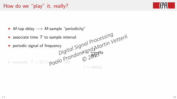
How do we “play” it, really?
◮ M-tap delay −→ M-sample “periodicity”
◮ associate time T to sample interval
◮ periodic signal of frequency
f =1
MTHz
◮ example: T = 22.7µs, M = 100f ≈ 440Hz
2.3 69
Digital Signal Processing
Paolo Prandoni and Martin Vetterli
© 2013

How do we “play” it, really?
◮ M-tap delay −→ M-sample “periodicity”
◮ associate time T to sample interval
◮ periodic signal of frequency
f =1
MTHz
◮ example: T = 22.7µs, M = 100f ≈ 440Hz
2.3 69
Digital Signal Processing
Paolo Prandoni and Martin Vetterli
© 2013
How do we “play” it, really?
◮ M-tap delay −→ M-sample “periodicity”
◮ associate time T to sample interval
◮ periodic signal of frequency
f =1
MTHz
◮ example: T = 22.7µs, M = 100f ≈ 440Hz
2.3 69
Digital Signal Processing
Paolo Prandoni and Martin Vetterli
© 2013

How do we “play” it, really?
◮ M-tap delay −→ M-sample “periodicity”
◮ associate time T to sample interval
◮ periodic signal of frequency
f =1
MTHz
◮ example: T = 22.7µs, M = 100f ≈ 440Hz
2.3 69
Digital Signal Processing
Paolo Prandoni and Martin Vetterli
© 2013

Playing a sine wave
M = 100, α = 1, x̄ [n] = sin(2π n/100) for 0 ≤ n < 100 and zero elsewhere
b bb bb bb bb bb bb b bb b bb b b b b b
b b b b b b b b b b b b b b b b b b b b b b b b b b b b b b b b b b b b b b b b b b b b b b b b b b b b b b b b b bb b bb b bb bb bb bb bb bb bb
0 16 32 48 64 80 96
−1
0
1
2.3 70
Digital Signal Processing
Paolo Prandoni and Martin Vetterli
© 2013

Playing a sine wave
M = 100, α = 1, x̄ [n] = sin(2π n/100) for 0 ≤ n < 100 and zero elsewhere
b bb bb bb bb bb bb b bb b bb b b b b b
b b b b b b b b b b b b b b b b b b b b b b b b b b b b b b b b b b b b b b b b b b b b b b b b b b b b b b b b b bb b bb b bb bb bb bb bb bb bb
0 16 32 48 64 80 96
−1
0
1
0 166 332 498 664 830 996
−1
0
1
2.3 70
Digital Signal Processing
Paolo Prandoni and Martin Vetterli
© 2013

Introducing some realism
◮ M controls frequency (pitch)
◮ α controls envelope (decay)
◮ x̄ [n] controls color (timbre)
2.3 71
Digital Signal Processing
Paolo Prandoni and Martin Vetterli
© 2013
Introducing some realism
◮ M controls frequency (pitch)
◮ α controls envelope (decay)
◮ x̄ [n] controls color (timbre)
2.3 71
Digital Signal Processing
Paolo Prandoni and Martin Vetterli
© 2013

Introducing some realism
◮ M controls frequency (pitch)
◮ α controls envelope (decay)
◮ x̄ [n] controls color (timbre)
2.3 71
Digital Signal Processing
Paolo Prandoni and Martin Vetterli
© 2013

A proto-violin
M = 100, α = 0.95, x̄ [n]: zero-mean sawtooth wave between 0 and 99, zero elsewhere
b b b b bb b b b bb b b b bb b b b bb b b b bb b b b bb b b b bb b b b bb b b b bb b b b bb b b b bb b b b bb b b b bb b b b bb b b b bb b b b bb b b b bb b b b bb b b b bb b b b bb
0 16 32 48 64 80 96
−1
0
1
2.3 72
Digital Signal Processing
Paolo Prandoni and Martin Vetterli
© 2013

A proto-violin
M = 100, α = 0.95, x̄ [n]: zero-mean sawtooth wave between 0 and 99, zero elsewhere
b b b b bb b b b bb b b b bb b b b bb b b b bb b b b bb b b b bb b b b bb b b b bb b b b bb b b b bb b b b bb b b b bb b b b bb b b b bb b b b bb b b b bb b b b bb b b b bb b b b bb
0 16 32 48 64 80 96
−1
0
1
0 166 332 498 664 830 996
−1
0
1
2.3 72
Digital Signal Processing
Paolo Prandoni and Martin Vetterli
© 2013

The Karplus-Strong Algorithm
M = 100, α = 0.9, x̄ [n]: 100 random values between 0 and 99, zero elsewhere
b
b
b
b bb
b
b
b
b
bb
b
b
b
b
b
b
b
b bb
b
b
b
b
b
b
b
b
b b
bbb
b
b
b b
b
b
b
b
b
b
b
b
b
b
b
bb
b b
bb
b
b
b
b
bb
bb
b
b
b bb bb
b
b
b
b
b b
b
b
b
b
b
b
b
b
b
b
b bb
b
bb
b
b
b
bb
b
b
b
0 16 32 48 64 80 96
−1
0
1
2.3 73
Digital Signal Processing
Paolo Prandoni and Martin Vetterli
© 2013

The Karplus-Strong Algorithm
M = 100, α = 0.9, x̄ [n]: 100 random values between 0 and 99, zero elsewhere
b
b
b
b
b
b
b
b
b
b
b
b
b
b
b
b
b
b
b
bb
b b
b
b
b
b
b
b
b
b
b
bb b
b
b
b
b
b
bb
b
b
b
b b
b
b
b
b
b
b
b
bb
b
b
b
b
b
b
b
b
b
b
b
b
b
b
b
b
b
b
b
b
b
b
b
b
b bb
b
b
b
b b
b
b
b
b
b b
b
b
b
b
b b
b
0 16 32 48 64 80 96
−1
0
1 b b
b
b
b
b
b
b
b
b
b
b
b
b
b
b
b
bb
b b
b
b
b
b
b
b
b
b
b
bb
b
b
b
b b
bbb
b
b
bb
b
b b
b
b
b b
bb
b
b
b
b
b
b
bb
b b
b
b
b
bb b
b
b
b
b b
b
b
b
b b
b
b
b
b
b b
b b
b
b
b
b
b
b
b
b
b
b
b
b
b
b b
b
b
b
b
b
b
b
b
b
b
b
b
b
b
b
bb
b b
b
b
b
b
b
b
b
b
b
bb
b
b
b
b b
b bb
b
b
bb
b
b b
b
b
b b
bb
b
b
b
b
b
b
bb
b b
b
b
b
bb bb
b
b
b b
b
b
b
b b
b
b
b
bb b
b b
b
b
b
b
b
b
b
b
b
b
b
b
b
b b
b
b
b
b
b
b
bb
b
b
b
b
b
b
b
bb
b b
b
b
b
b
b
b
b
b
b
bb
b
b
b
b b
b bb
b
b
bb
b
b b
b
b
b b
bb
b
b
b
b
b
b
bb
b b
b
b
b
bb bb
b
b
b b
b
b
b
b b
bb
b
bb b
b b
b
b
b
b
b
b
b
b
b
b
b
b
b
b b
b
b
b
b
b
b
bb
b
b
b
b
b
b
b
bb
b bb
b
b
b
b
b
b
b
b
bb
b
b
b
b b
b bb
b
b
b b
b
b b
b
b
b b
bb
b
b
b
bbb
bb
b b
b
b
b
bb bb
b
b
b b
b
b
b
b b
bb
b
bb b
b b
b
b
b
b
b
b
b
bb
b
b
b
b
b b
b
b
b
b
b
b
bb
b
b
b
b
b
b
b
bbb bb
b
b
b
b
b
b
b
b
bb
b
b
b
b b
b bb
b
b
b b
b
b b
b
b
b b
bb
b
b
b
bbb
bb
b b
b
b
b
bb bb
b
b
b b
b
b
b
b b
bb
b
bb b
b b
b
b
b
b
b
b
b
bb
b
b
b
b
b b
b
b
b
b
b
b
bb
b
b
b
b
b
b
b
b bb bb
b
bb
b
b
b
b
b
bb
b
b
b
b b
b bb
b
b
b b
b
b bb
b
b b
bb
b
b
b
bbb
bb
b b
b
b
b
bb bb
b
b
b b
b
b
bb b
bbb
bb b
b b
b
b
b
b
b
bb
bb
b
b
b
b
b b
b
b
b
b
b
b
bb
b
b
bb
bb
b
b bb bb
b
bb
b
b
b
b
b
bb
b
b
b
b b
b bb
b
b
b b
b
b bb
b
b b
bb
b
b
b
bbb
bb
b b
b
b
b
bb b b
b
b
b b
b
b
bb b
bbb
bb b
b b
b
b
b
b
b
bb
bb
b
b
b
b
b b
b
b
b
b
b
b
bb
b
b
bb
bbb
b b b bbb
bb
b
b
b
b
b
bb
b
b
b
b b
b bb
b
b
b b
b
b bb
b
b b
bb
b
b
b
bbb
bb
b b
bb
b
bb b b
b
b
b b
bb
bb b
bbb
bb b
b b
b
b
b
b
b
bb
bb
b
b
b
b
b b
b
b
b
b
b
b
bb
b
bbb
bbb
b b b bbb
bb
b
b
b
b
b
bb
b
bb
b b
b bb
b
b
b b
b
b bb
bb b
bb
bb
b
bbb
bb
b b
bb
bb b b b
b
b
b b
bb
bb b
bbb
bb b
b b
b
b
b
b
b
bb
bb
bb
b
b
b b
b
b
b
b
b
b
bbb
bbb
bbb
b b b bbb
bb
b
b
b
b
b
b b
b
bb
b b
b bb
b
b
b b
b
b bb
bb b
b b
bb
b
bbb
b b
b b
bb
bb b b b
b
b
b b
bb
bb b
bbb
b bb
b b
b
b
b
b
b
bbbb
bb
b
b
b
0 166 332 498 664 830 996
−1
0
1
2.3 73
Digital Signal Processing
Paolo Prandoni and Martin Vetterli
© 2013

Recap
◮ We have seen basic elements:
• adders
• multipliers
• delays
◮ We have seen two systems
• moving averages
• recursive systems
◮ We were able to build simple systems with interesting properties
◮ to understand all of this in more details we need a mathematical framework!
2.3 74
Digital Signal Processing
Paolo Prandoni and Martin Vetterli
© 2013

END OF MODULE 2.3
Digital Signal Processing
Paolo Prandoni and Martin Vetterli
© 2013

w
Digital Signal Processing
Paolo Prandoni and Martin Vetterli
© 2013

END OF MODULE 2
2.3 74
Digital Signal Processing
Paolo Prandoni and Martin Vetterli
© 2013

Exercises (2.1)
Q1 Sketch the signal u[n − 1]
Q2 Sketch the signal u[n]− u[n − 4]
Q3 Prove that
x [n] =∞∑
k=−∞
x [k]δ[n − k]
Q4 Prove that
u[n] =
n∑
k=−∞
δ[k]
2.3 75
Digital Signal Processing
Paolo Prandoni and Martin Vetterli
© 2013

Answers: Q1
x [n] = u[n]
b b b b b b b b b b b b b b b b
b b b b b b b b b b b b b b b b b
−15 −10 −5 0 5 10 150
1
2.3 76
Digital Signal Processing
Paolo Prandoni and Martin Vetterli
© 2013

Answers: Q1
x [n] = u[n − 1]
b b b b b b b b b b b b b b b b b
b b b b b b b b b b b b b b b b
−15 −10 −5 0 5 10 150
1
2.3 76
Digital Signal Processing
Paolo Prandoni and Martin Vetterli
© 2013

Answers: Q2
x [n] = u[n]− u[n − 4]
b b b b b b b b b b b b b b b b
b b b b b b b b b b b b b b b b b
−15 −10 −5 0 5 10 15
−1
0
1
2.3 77
Digital Signal Processing
Paolo Prandoni and Martin Vetterli
© 2013

Answers: Q2
x [n] = u[n]− u[n − 4]
b b b b b b b b b b b b b b b b
b b b b b b b b b b b b b b b b b
b b b b b b b b b b b b b b b b b b b b
b b b b b b b b b b b b b
−15 −10 −5 0 5 10 15
−1
0
1
2.3 77
Digital Signal Processing
Paolo Prandoni and Martin Vetterli
© 2013

Answers: Q2
x [n] = u[n]− u[n − 4]
b b b b b b b b b b b b b b b b
b b b b
b b b b b b b b b b b b b
−15 −10 −5 0 5 10 15
−1
0
1
2.3 77
Digital Signal Processing
Paolo Prandoni and Martin Vetterli
© 2013

Answers: Q3
x [n] =∞∑
k=−∞
x [k]δ[n − k]
δ[n − k] =
1 if n = k
0 otherwise
n ∈ Z
Therefore, the only term in the sum that is not “killed” is the one for k = n, i.e. x [n].
2.3 78
Digital Signal Processing
Paolo Prandoni and Martin Vetterli
© 2013

Answers: Q4
u[n] =
n∑
k=−∞
δ[k]
Call y [n] =∑n
k=−∞δ[k].
If n < 0 all the terms in the sum are zero, so y [n] = 0 for n < 0If n > 0, the sum will have just one nonzero term for k = 0, so y [n] = 1 for n ≥ 0.Therefore y [n] = u[n]
2.3 79
Digital Signal Processing
Paolo Prandoni and Martin Vetterli
© 2013
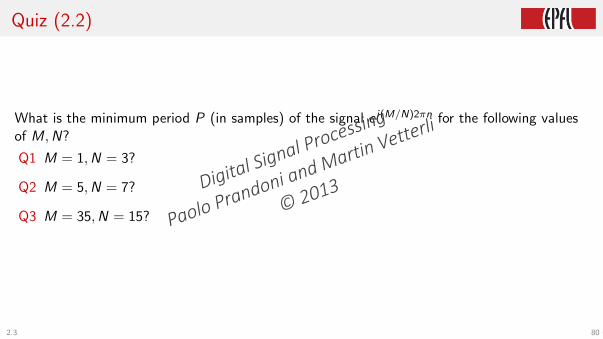
Quiz (2.2)
What is the minimum period P (in samples) of the signal e j(M/N)2πn for the following valuesof M,N?
Q1 M = 1,N = 3?
Q2 M = 5,N = 7?
Q3 M = 35,N = 15?
2.3 80
Digital Signal Processing
Paolo Prandoni and Martin Vetterli
© 2013

Answers
Q1 P = 3
Q2 P = 7
Q3 P = 3
2.3 81
Digital Signal Processing
Paolo Prandoni and Martin Vetterli
© 2013

Quiz (2.3)
Compute the moving average for the signal
x [n] = δ[n] + 2δ[n − 1] + 3δ[n − 2]
2.3 82
Digital Signal Processing
Paolo Prandoni and Martin Vetterli
© 2013

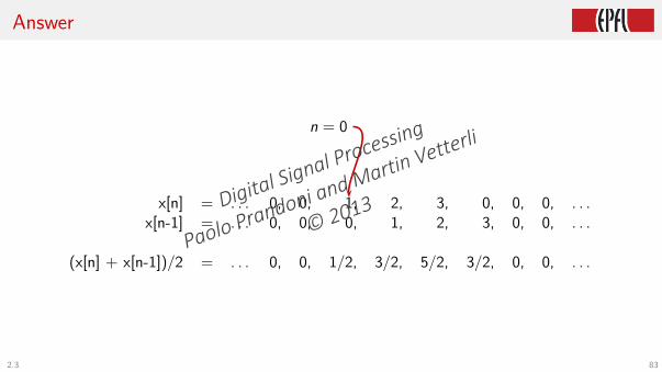
Answer
n = 0
x[n] = . . . 0, 0, 1, 2, 3, 0, 0, 0, . . .x[n-1] = . . . 0, 0, 0, 1, 2, 3, 0, 0, . . .
(x[n] + x[n-1])/2 = . . . 0, 0, 1/2, 3/2, 5/2, 3/2, 0, 0, . . .
2.3 83
Digital Signal Processing
Paolo Prandoni and Martin Vetterli
© 2013
Answer
n = 0
x[n] = . . . 0, 0, 1, 2, 3, 0, 0, 0, . . .x[n-1] = . . . 0, 0, 0, 1, 2, 3, 0, 0, . . .
(x[n] + x[n-1])/2 = . . . 0, 0, 1/2, 3/2, 5/2, 3/2, 0, 0, . . .
2.3 83
Digital Signal Processing
Paolo Prandoni and Martin Vetterli
© 2013

Answer
y [n] =
0 for n < 01/2 for n = 03/2 for n = 15/2 for n = 23/2 for n = 30 for n > 3
2.3 84
Digital Signal Processing
Paolo Prandoni and Martin Vetterli
© 2013

Quiz (2.3)
Compute the output of the system below when the input is
x [n] = δ[n] + 2δ[n − 1] + 3δ[n − 2]
x [n] + b y [n]
z−11/2
2.3 85
Digital Signal Processing
Paolo Prandoni and Martin Vetterli
© 2013

Answer
y [n] = 0 for n < 0
y [0] = x [0] + y [−1]/2 = 1
y [1] = x [1] + y [0]/2 = 2 + 0.5 = 2.5
y [2] = x [2] + y [1]/2 = 3 + 1.25 = 4.25
y [3] = x [3] + y [2]/2 = 0 + 2.175
. . .
y [n] = 4.25 · (0.5)n−2 for n ≥ 2
2.3 86
Digital Signal Processing
Paolo Prandoni and Martin Vetterli
© 2013
Quizzes
Q1 Write the recursive equation for the KS algorithm
Q2 A major reason for using the KS algorithm is that it is simple since it uses onemultiplication and addition per output sample. However, it requires M memory elements!Suggest an architecture for the violin synthesis which uses only M/2 memory elementsand write out an example for a small M, like M = 8.
Hint: Use M even, and think of up- and down-triangles!
2.3 87
Digital Signal Processing
Paolo Prandoni and Martin Vetterli
© 2013

Answers to questions
A1: yn = αyn−M+1 + xn
A2: Use the idea is that a single triangle can be used with alternating signs.
x [n] + b y [n]
z−M−1
For ex., for a period of 8 samples, M = 4, xn = 0, 1, 2, 1 and α = 1yn = 0, 1, 2, 1, 0,−1,−2,−1, 0, 1, 2, ....
2.3 88
Digital Signal Processing
Paolo Prandoni and Martin Vetterli
© 2013