rCRF: Recursive Belief Estimation over CRFs in

RGB-D Activity Videos

Ozan Sener

School of Electrical & Computer Eng.

Cornell University

Ashutosh Saxena

Department of Computer Science

Cornell University

Abstract—For assistive robots, anticipating the future actionsof humans is an essential task. This requires modelling both theevolution of the activities over time and the rich relationshipsbetween humans and the objects. Since the future activities ofhumans are quite ambiguous, robots need to assess all the futurepossibilities in order to choose an appropriate action. Therefore,a successful anticipation algorithm needs to compute all plausiblefuture activities and their corresponding probabilities.

In this paper, we address the problem of efficiently computingbeliefs over future human activities from RGB-D videos. Wepresent a new recursive algorithm that we call Recursive Con-ditional Random Field (rCRF) which can compute an accuratebelief over a temporal CRF model. We use the rich modellingpower of CRFs and describe a computationally tractable in-ference algorithm based on Bayesian filtering and structureddiversity. In our experiments, we show that incorporating belief,computed via our approach, significantly outperforms the state-of-the-art methods, in terms of accuracy and computation time.

I. INTRODUCTION

Understanding human activities is an important skill for

robots working with humans. Robots not only need to de-

tect the activity that human is performing but also need to

anticipate what activity can a human possibly perform in the

near future in order to choose the right actions. Anticipation

ability is especially important for assistive robots, and we have

recently seen many successful collaborative robotics applica-

tions [44, 29, 21] using the most likely action(s) humans might

take in near future. The set of the future possibilities is quite

large, and robots need to be aware of all of them in addition

to the most likely one. In this work, we focus on estimating

the set of all possible future states with their likelihoods.

Anticipation is a challenging task, and it requires us to

model the relationships between several objects and the hu-

man(s) in the scene, as well as their temporal evolution. Al-

though the modelling assumptions and model parametrization

varies, the common approach [22, 17, 23, 26] is using Con-

ditional Random Field (CRF) to represent the rich relations

in the scene, and anticipating a single or a few most likely

future states. Since the future is ambiguous, the most likely

state might not be sufficient enough to assess the risk of each

action. For example, consider a collaborative cooking scenario,

the object that human is reaching is typically a distribution

over many objects. Computing the trajectory, that is least likely

to conflict with the human, is only possible via consideration

of all future possibilities. The question, we address in this

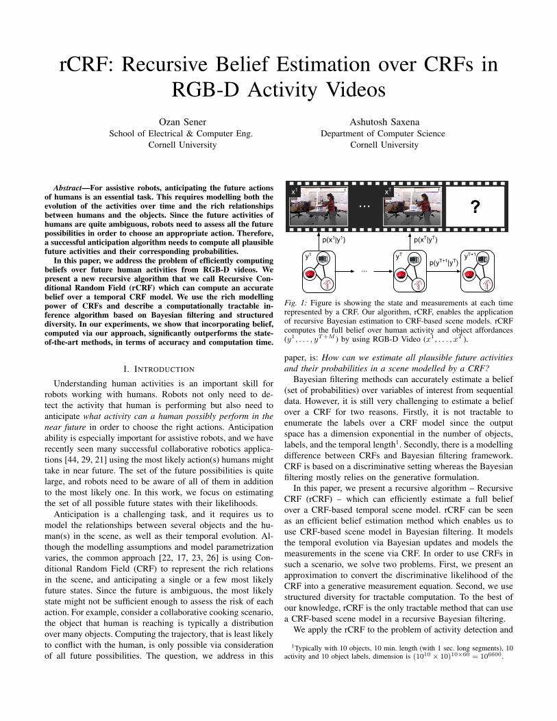
p(yT+1|yT)yT+1

...

...x1 xT

p(x1|y1) p(xT|yT)

yTy1

Fig. 1: Figure is showing the state and measurements at each timerepresented by a CRF. Our algorithm, rCRF, enables the applicationof recursive Bayesian estimation to CRF-based scene models. rCRFcomputes the full belief over human activity and object affordances(y1, . . . , yT+M ) by using RGB-D Video (x1, . . . , xT ).

paper, is: How can we estimate all plausible future activities

and their probabilities in a scene modelled by a CRF?

Bayesian filtering methods can accurately estimate a belief

(set of probabilities) over variables of interest from sequential

data. However, it is still very challenging to estimate a belief

over a CRF for two reasons. Firstly, it is not tractable to

enumerate the labels over a CRF model since the output

space has a dimension exponential in the number of objects,

labels, and the temporal length1. Secondly, there is a modelling

difference between CRFs and Bayesian filtering framework.

CRF is based on a discriminative setting whereas the Bayesian

filtering mostly relies on the generative formulation.

In this paper, we present a recursive algorithm – Recursive

CRF (rCRF) – which can efficiently estimate a full belief

over a CRF-based temporal scene model. rCRF can be seen

as an efficient belief estimation method which enables us to

use CRF-based scene model in Bayesian filtering. It models

the temporal evolution via Bayesian updates and models the

measurements in the scene via CRF. In order to use CRFs in

such a scenario, we solve two problems. First, we present an

approximation to convert the discriminative likelihood of the

CRF into a generative measurement equation. Second, we use

structured diversity for tractable computation. To the best of

our knowledge, rCRF is the only tractable method that can use

a CRF-based scene model in a recursive Bayesian filtering.

We apply the rCRF to the problem of activity detection and

1Typically with 10 objects, 10 min. length (with 1 sec. long segments), 10activity and 10 object labels, dimension is (1010 × 10)10×60 = 106600.

anticipation from RGB-D data. As a CRF-based scene model,

we use the model from [24] which represents the scene as a

CRF over human activity and object affordances. We then use

the RGB-D video to detect and anticipate activities via rCRF.

Our experiments show that we outperform the state-of-the-

art methods for detection and anticipation, and the improve-

ment in the anticipation accuracy is significant. In addition to

the improvements in accuracy, we show that our anticipation

also improves the computation time and runs near real-time.

In summary, the contributions of this work are:

• We present Recursive-CRF (rCRF) method that uses the

rich modeling power of CRF in Bayesian filtering setting.

• We present a structured-diversity based approach to en-

able tractable computation of the belief.

• We apply our rCRF method to the problem of activity

detection and anticipation in RGB-D videos.

II. BACKGROUND AND RELATED WORK

Bayesian Recursive Filtering: Estimating a belief over vari-

ables of interest from partial observations is a widely studied

problem [41]. Sequential Monte Carlo (SMC) —aka par-

ticle filter— is typically used to estimate beliefs in high-

dimensional cases. SMC methods represent the belief as a set

of samples and we refer the reader to [5] for rigorous analysis.

SMC methods are not directly applicable to spaces like

CRF since the number of samples required is intractably

high. One solution to this problem is the Rao-Blackwellised

particle filter [6]. It uses a partition of the state variables y

into two set of variables y1 and y2 such that the variables

in one partition y2 can be estimated using the partition y1.

Then Rao-Blackwellised particle filter [6] estimates the y1 via

SMC and directly estimates y2 using y1. However, for our

problem, we are not aware of any state decomposition which

enables Rao-Blackwellised particle filter. Although there are

discrimantive extensions of Bayesian models like recursive

least squares[37], in this paper we only consider the states

represented by CRFs. Moreover, we are not aware of any

Bayesian smoothing formulation applied over CRFs.

One tractable application of the SMC framework to the

CRF based scene analysis problems is the ATCRF [22] model.

ATCRF [22] uses a set of heuristics to sample the parti-

cles. However, ATCRF faces the problem of computational

limitations and requires computationally intractable number

of samples for anticipation. We follow the Bayesian filtering

theory and efficiently estimate the belief.

Structured Diversity and Variants of CRFs: CRFs are

widely used to solve activity analysis problems [39, 33] in a

discriminative setting. CRF models the conditional likelihood

of the state given the observations, and the MAP solution can

be found. Although this setting is powerful, it does not give

any information about the belief other than the MAP state.

Other than the MAP solution, it is also tractable to compute

the modes of the CRF [1, 27, 3]. These modes can be

considered as an approximate state space, and the belief can

be computed only for them. Indeed, this claim is empirically

validated in many problems like parameter learning [31],

empirical MBR [32] and discrimantive re-ranking [45].

Among the aforementioned approaches, Div-M-Best [1] is

a method applicable to the sequential information. [1] starts

by dividing the video into a set of frames and computes

the diverse-most-likely solutions of each frame independently.

Then, it combines the results via the temporal relations. On

the contrary, we formulate the problem as recursive Bayesian

smoothing and compute the samples based on temporal re-

lations. Formally, given state variables y1, . . . ,yT and ob-

servations x1, . . . ,xT , we directly sample p(yt|x1, . . . ,xT ),whereas, [1] samples p(yt|xt). Since our sampling procedure

uses the entire video, our samples are more accurate.

There are variants of CRFs that rely on sequential models

as well such as, Dynamic CRF (dCRF) [40], Infinite Hidden

CRF [2], Gaussian Process Latent CRF [17] and Hierarchical

Semi-Markov CRF (HSCRF). Although they are applicable to

videos, we are not aware of any tractable method to compute

a belief over any of the aforementioned graphical model.

DCRF [43] learns the observation likelihood –p(xt|yt)–by using the low-dimensional nature of the features and

follows Bayesian filtering. Since our features have very high-

dimension (for N objects, we have 58N + 20N2 + 103dimensional features), DCRF [43] is not directly applicable.

However, it is possible to learn p(yt|xt) and approximately

use the DCRF formulation by assuming observation and

label likelihoods are equal. Moreover, This approach can be

shown equivalent to finding local maximum of energy function

defined by [24] following the formulation of Fox et al [8].

It is also common to compute a belief over latent nodes as

in the case of infinte hidden CRF [2] and Gaussian Process

Latent CRF[17]. However, they are not directly applicable

to our problem since they can compute a belief only over

the latent node. CRF-Filter [28] is a closely related approach

which uses CRFs in a particle filtering scenario. However, it

is based on sampling of a low dimensional state space and it

is not applicable to our rich model either.

Human Activity Detection and Anticipation: Early works

relied solely on human poses. These works range from jointly

segmenting and recognizing sub-activities [14, 38] to choosing

a relevant model out of activity models [30]. Main limitation of

these methods is that they do not use the object information.

Some methods successfully model and use the relations of

the human-poses and objects in the scene [11, 46, 18, 19].

However, a significant drawback of these works is missing the

fact that object affordance is more important than object types

for activities [10]. Indeed, object affordance based models

had higher performance (e.g., [24]). A recent work modelled

human activities with latent models [15] and also handled the

disagreements among the activity annotations [16].

Another drawback of these methods is the requirement of

the entire activity. Detecting the activity in its early stages

is especially crucial for assistive robotics and surveillance

systems. Although a few recent work adress the problem of

activity detection with partial/early information [13, 36], these

works do not perform anticipation. There are a few recent

Frame t

Posterior CRFp(yt-1|x1,...,xT)

Resampling

Movable

Openable Opening

p=0.3

Forward Messagesɑt+1(yt+1)

Frame t+1

p(yt+1|xt+1)

Posterior CRFp(yt+1|x1,...,xT)

Resampling

Movable

Movable Cleaning

p=0.15 Stirrable

Openable Stirring

p=0.05

Stationary

Openable Opening

p=0.8

Backward Messages

βt(yt)

Backward Messages

βt-1(yt-1)

p=0.1 Movable

MovingStationary

p=0.6 Reachable

ReachingStationary

Belief p(yt-1 |x1,...,xT)

...

Forward Messages

αt(yt)

CRFlikelihood

p=0.15 Stationary

ReachingReachable

p=0.7 Stationary

ClosingClosable

Belief p(yt |x1,...,xT)

...Frame t-1 Frame t

p(yt-1|xt-1) p(yt|xt) CRFlikelihood

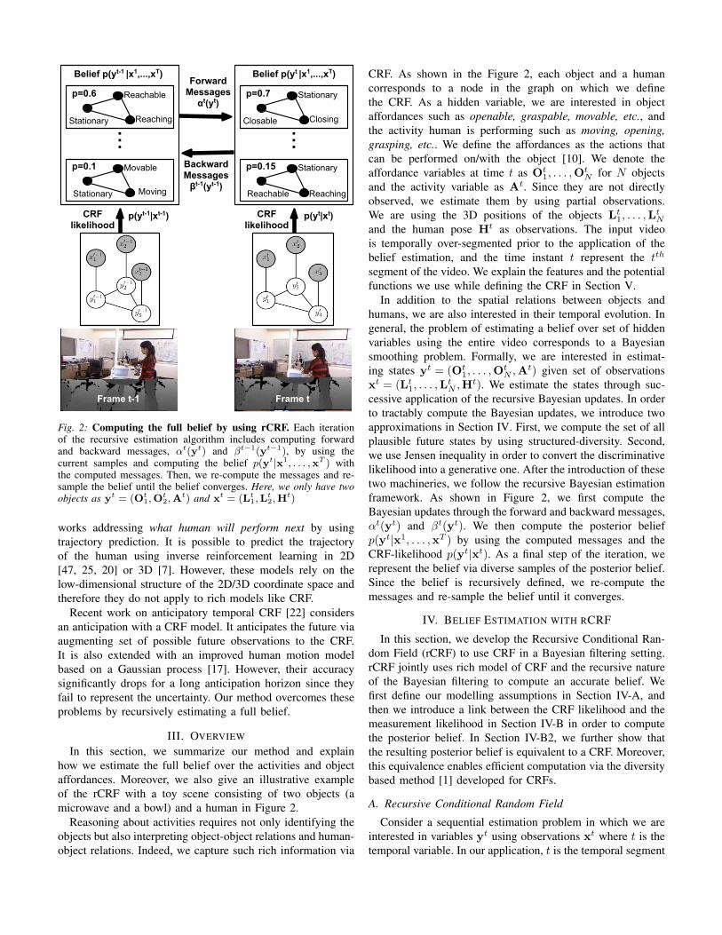
Fig. 2: Computing the full belief by using rCRF. Each iterationof the recursive estimation algorithm includes computing forwardand backward messages, αt(yt) and βt−1(yt−1), by using thecurrent samples and computing the belief p(yt|x1, . . . ,xT ) withthe computed messages. Then, we re-compute the messages and re-sample the belief until the belief converges. Here, we only have twoobjects as yt = (Ot

1,Ot2,A

t) and xt = (Lt1,L

t2,H

t)

works addressing what human will perform next by using

trajectory prediction. It is possible to predict the trajectory

of the human using inverse reinforcement learning in 2D

[47, 25, 20] or 3D [7]. However, these models rely on the

low-dimensional structure of the 2D/3D coordinate space and

therefore they do not apply to rich models like CRF.

Recent work on anticipatory temporal CRF [22] considers

an anticipation with a CRF model. It anticipates the future via

augmenting set of possible future observations to the CRF.

It is also extended with an improved human motion model

based on a Gaussian process [17]. However, their accuracy

significantly drops for a long anticipation horizon since they

fail to represent the uncertainty. Our method overcomes these

problems by recursively estimating a full belief.

III. OVERVIEW

In this section, we summarize our method and explain

how we estimate the full belief over the activities and object

affordances. Moreover, we also give an illustrative example

of the rCRF with a toy scene consisting of two objects (a

microwave and a bowl) and a human in Figure 2.

Reasoning about activities requires not only identifying the

objects but also interpreting object-object relations and human-

object relations. Indeed, we capture such rich information via

CRF. As shown in the Figure 2, each object and a human

corresponds to a node in the graph on which we define

the CRF. As a hidden variable, we are interested in object

affordances such as openable, graspable, movable, etc., and

the activity human is performing such as moving, opening,

grasping, etc.. We define the affordances as the actions that

can be performed on/with the object [10]. We denote the

affordance variables at time t as Ot1, . . . ,O

tN for N objects

and the activity variable as At. Since they are not directly

observed, we estimate them by using partial observations.

We are using the 3D positions of the objects Lt1, . . . ,L

tN

and the human pose Ht as observations. The input video

is temporally over-segmented prior to the application of the

belief estimation, and the time instant t represent the tth

segment of the video. We explain the features and the potential

functions we use while defining the CRF in Section V.

In addition to the spatial relations between objects and

humans, we are also interested in their temporal evolution. In

general, the problem of estimating a belief over set of hidden

variables using the entire video corresponds to a Bayesian

smoothing problem. Formally, we are interested in estimat-

ing states yt = (Ot1, . . . ,O

tN ,At) given set of observations

xt = (Lt1, . . . ,L

tN ,Ht). We estimate the states through suc-

cessive application of the recursive Bayesian updates. In order

to tractably compute the Bayesian updates, we introduce two

approximations in Section IV. First, we compute the set of all

plausible future states by using structured-diversity. Second,

we use Jensen inequality in order to convert the discriminative

likelihood into a generative one. After the introduction of these

two machineries, we follow the recursive Bayesian estimation

framework. As shown in Figure 2, we first compute the

Bayesian updates through the forward and backward messages,

αt(yt) and βt(yt). We then compute the posterior belief

p(yt|x1, . . . ,xT ) by using the computed messages and the

CRF-likelihood p(yt|xt). As a final step of the iteration, we

represent the belief via diverse samples of the posterior belief.

Since the belief is recursively defined, we re-compute the

messages and re-sample the belief until it converges.

IV. BELIEF ESTIMATION WITH RCRF

In this section, we develop the Recursive Conditional Ran-

dom Field (rCRF) to use CRF in a Bayesian filtering setting.

rCRF jointly uses rich model of CRF and the recursive nature

of the Bayesian filtering to compute an accurate belief. We

first define our modelling assumptions in Section IV-A, and

then we introduce a link between the CRF likelihood and the

measurement likelihood in Section IV-B in order to compute

the posterior belief. In Section IV-B2, we further show that

the resulting posterior belief is equivalent to a CRF. Moreover,

this equivalence enables efficient computation via the diversity

based method [1] developed for CRFs.

A. Recursive Conditional Random Field

Consider a sequential estimation problem in which we are

interested in variables yt using observations xt where t is the

temporal variable. In our application, t is the temporal segment

id. We note RGB-D camera reading as xt, and object and

activity labels as yt. We now define the Recursive Conditional

Random Field (rCRF) framework for such a problem following

the assumptions of Hidden Markov Models.

Definition 1: Let Gt = (V t, Et) be set of graphs indexed

by the temporal variable t and yt is indexed by the vertices

of Gt as yt = (ytv)v∈V t . Then, (x1...T ,y1...T ) is a Recursive

Conditional Random Field with dynamics pv(·|·) when

1) For each t, (yt,xt) is a CRF over Gt = (V t, Et)2) p(yt|y1, . . . ,yt−1) = p(yt|yt−1) ∀t (Markov)

3) p(xt|y1, . . . ,yt,x1, . . . ,xt−1) = p(xt|yt) ∀t4) p(yt = y|yt−1 = y′) = pv(y|y

′) (stationarity)

�

yt−1

yt

yt+1

xt+12

xt+13

yt−13

yt+12

xt−11

xt−12

xt+11

xt−13

yt+11y

t−11

yt+13

xt

1

xt

2

xt

3

yt

1

yt−12

yt

3

yt

2

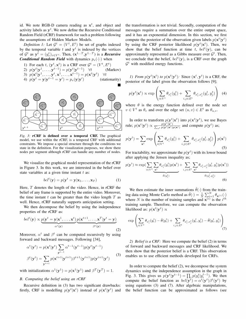
Fig. 3: rCRF is defined over a temporal CRF. The graphicalmodel, we use within the rCRF, is a temporal CRF with additionalconstraints. We impose a special structure through the conditions westate in the definition. For the visualization purposes, we show therenodes per segment although rCRF can handle any number of nodes.

We visualize the graphical model representation of the rCRF

in Figure 3. In this work, we are interested in the belief over

state variables at a given time instant t as:

belt(y) = p(yt = y|x1, . . . ,xT ) (1)

Here, T denotes the length of the video. Hence, in rCRF the

belief of any frame is supported by the entire video. Moreover,

the time instant t can be greater than the video length T as

well. Hence, rCRF naturally supports anticipation setting.

We then decompose the belief by using the independence

properties of the rCRF as:

belt(y) ∝ p(yt = y|x1, . . . ,xt)︸ ︷︷ ︸

αt(y)

p(xt+1, . . . ,xT |yt = y)︸ ︷︷ ︸

βt(y)

(2)

Moreover, αt and βt can be computed recursively by using

forward and backward messages. Following [34],

αt(yt) = p(xt|yt)∑

yt−1

αt−1(yt−1)p(yt|yt−1)

βt(yt) =∑

yt+1

p(xt+1|yt+1)βt+1(yt+1)p(yt+1|yt)(3)

with initializations α1(y1) = p(x1|y1) and βT (yT ) = 1.

B. Computing the belief using an rCRF

Recursive definition in (3) has two significant drawbacks:

firstly, CRF is modelling p(yt|xt) instead of p(xt|yt) and

the transformation is not trivial. Secondly, computation of the

messages require a summation over the entire output space,

and it has an exponential dimension. In this section, we first

compute the posterior of the observation given labels p(xt|yt)by using the CRF posterior likelihood p(yt|xt). Then, we

show that the belief function at time t, belt(y), can be

approximately represented as a Gibbs measure over Gt. Then,

we conclude that the belief, belt(y), is a CRF over the graph

Gt with modified energy functions.

1) From p(yt|xt) to p(xt|yt): Since (xt,yt) is a CRF, the

posterior of the label given the observation follows [9];

p(yt|xt) ∝ exp

∑

i∈V t

θxti(yti) +

∑

i,j∈Et

θxti,xt

j(yti , y

tj)

(4)

where θ is the energy function defined over the node set

v ∈ V t as θv and over the edge set (u, v) ∈ Et as θu,v .

In order to transform p(yt|xt) into p(xt|yt), we use Bayes

rule; p(xt|yt) ∝ p(yt|xt)∑xt p(yt|xt)p(xt) and compute p(yt) as;

p(yt) =∑

xt

exp

∑

i∈V t

θxti(yti) +

∑

i,j∈Et

θxti,xt

j(yti , y

tj)

p(xt)

(5)

For tractability, we approximate the p(yt) with its lower bound

after applying the Jensen inequality as;

p(yt) ≈ exp(∑

i∈V t

∑

xt

θxti(yt

i)p(xt)

︸ ︷︷ ︸

θ(yti)

+∑

i,j∈Et

∑

xt

θxti,xt

j(yt

i , ytj)p(x

t)

︸ ︷︷ ︸

θ(yti,yt

j)

)

(6)

We then estimate the inner summations θ(·) from the train-

ing data using Monte Carlo method as θ(·) = 1N

∑N

i=1 θx(i)(·)where N is the number of training samples and x(i) is the ith

training sample. Therefore, we can compute the observation

likelihood as: p(xt|yt) ∝

exp

∑

i∈V t

θxti(yt

i)− θ(yti) +

∑

i,j∈Et

θxti,xt

j(yt

i , ytj)− θ(yt

i , ytj)

(7)

2) Belief is a CRF: Here we compute the belief (2) in terms

of forward and backward messages and CRF likelihood. We

then show that the posterior belief is a CRF. This observation

enables us to use efficient methods developed for CRFs.

In order to compute the belief (2), we decompose the system

dynamics using the independence assumption in the graph in

Fig. 3. This gives us p(yt|yt−1) =∏

i p(yti |y

t−1i ). We then

compute the belief function as bel(yt) = αt(yt)βt(yt) by

using equations (3) and (7). After algebraic manipulations,

the belief function can be approximated as follows (see

supplementary material for a detailed derivation):

bel(yt) ∝ exp

∑

i,j∈Et

(

θxti,xt

j(yt

i , ytj)− θ(yt

i , ytj))

∑

i∈V t

θxti(yt

i)− θ(yti) +

∑

yt−1

αt−1(yt−1) log p(yt

i |yt−1i )

+1

γ

∑

yt+1

βt+1(yt+1)p(xt+1|yt+1) log p(yt+1

i |yti)

(8)

where γ =∑

yt+1 βt+1(yt+1)p(xt+1|yt+1)One property to observe is the decomposition of the belief

over the graph. Resulting belief function, (8), is a summation

over energy terms defined over nodes i ∈ V t and edges

i, j ∈ Et. Hence, belief belt(·) is a Gibbs measure over Gt. By

using Hammersley-Clifford theorem [12], we conclude that the

posterior belief in rCRF is also a CRF. In other words, belief

is a CRF defined over the same graph with a modified energy.

3) Belief via Diverse-Most-Likely Samples: Since we com-

puted the belief function and showed that it is equivalent to a

CRF, we now need an efficient method for computing it.

We follow the observation that CRF-likelihood over a nat-

ural scene concentrates on a few diverse samples [1] because

each scene only has a few plausible explanation. So, we

compute the belief for only those samples. In other words,

let’s assume the set of all plausible solutions at time t is

Yt = yt,1, . . . ,yt,M where yt,i is the ith sample at time

t. We then redefine the belief as;

approx belt(y) =

{belt(y)∑

y′∈Yt belt(y′) if y ∈ Yt

0 o.w.(9)

Since there are only a few plausible explanation of a visual

observation and CRF-based belief concentrates only on those

samples, proper selection of the samples Yt is expected to

work well in practice. These samples are typically selected as

the diverse-most-likely solutions of the CRF. They are most-

likely samples because we are only interested in the plausible

explanations. They are diverse because we are interested in the

modes of the CRF other than set of samples around the MAP

solution. Diversity is achieved via asserting samples to be at

least δ unit apart from each other via the distance function ∆(we use hamming distance as a in our experiments). In other

words, we solve the following optimization problem in order

to get the samples which represent the belief;

yt,i = argmaxy belt(y)

s.t. ∆(y,yt,j) ≥ δ ∀ j < i(10)

This optimization is NP-hard in general; however, since we

already showed belt(y) is CRF, we use the existing diverse-

m-best algorithms developed for CRFs. We use the Lagrange

relaxation by Batra et al. [1]. We explain the details of solving

this problem by using [1] in supplementary material.

In summary, we first compute the belief via (8) for all

frames by using samples of the previous and the next frame

as well as CRF likelihoods. Then, we compute the diverse

samples of (8) by using [1]. After computing the samples, we

compute the messages αt and βt by using the equations (7)

and (3). We continue to re-sample the beliefs and re-compute

the messages recursively until the convergence. Moreover,

during the initialization, we only sample the observation

function (7) since the messages are not available.

V. HUMAN ACTIVITY DETECTION AND ANTICIPATION

In this section, we describe how we apply the rCRF

framework to RGB-D videos for human activity detection and

anticipation. We are interested in activities such as reaching

and moving, and object affordances such as reachable and

movable as explained in Section III. We follow the approach

in [24], and start with temporally segmenting the video. This

step can be considered as an oversegmentation in the temporal

domain. It decreases the computation complexity and enables

using motion information as an observation.

We then obtain the observations xt = (Lt1, L

t2, H

t), by

detecting the objects in the first frame and then tracking

them. We obtain the human pose Ht through a skele-

ton tracker. We consider affordances and activities as state

yt = (Ot1, . . . , O

tN , A) where N is the number of objects.

We extracted set of features from the observations follow-

ing the feature functions in [24] (eg. relative and absolute

location of objects, human joints and their temporal displace-

ments). After extracting the features, we define our CRF

as a log-linear CRF and learn the energy function defined

in (4) by using the Structural SVM [42] as in the case of

[24]. We use the first order statistics for temporal dynam-

ics as pv(y, y′) = p(Y t

v = y|Y t−1v = y′) =

#(Y tv=y,Y t−1

v =y′)#(Y t

v=y′)

where #(·, ·) is number of the co-occurrence in training data.

After defining the observation, state and dynamics, we apply

the rCRF framework. We also summarize the activity detection

and anticipation application in Algorithm 1.

Algorithm 1 Compute belief the over (Ot1...N , At) for

t ∈ [1, T + τ ] in an RGB-D Video of length T

Initialization:

Compute Lt1, . . . , L

tN , and Ht for t ∈ [1, T ] via [24].

Compute p(Lt1...N , Ht|Ot

1...N , At) for t ∈ [1, T ] via (7)

Compute the belief via (8) w/o messages (α = 1, β = 1)

Detection:

repeat

for t ∈ [1, T ] do

Compute the forward/backward messages via (3)

Compute the belief via (8) an sample via (10)

end for

until convergence or number of iterations limit

Anticipation:

for t ∈ [T + 1, T + τ ] do

Compute only the forward messages via (3)

Sample the belief directly from the forward messages.

end for

Moreover, since the temporal relations are modeled as

causal, we do not compute the backward messages during the

anticipation. In anticipation, there is also no future observation.

Hence, the belief is defined solely by the forward messages.

In order to compute the belief for future frames, we propagate

the estimated belief. We propagate the belief to the next frame

by sampling the next state of the each sample in the belief of

the current frame via the temporal dynamics. Then, we choose

diverse most likely samples out of the propagated samples via

solving (10) with exhaustive search.

VI. EXPERIMENTAL RESULTS

In order to experimentally evaluate the proposed rCRF

model and the belief computation, we perform experiments on

two applications. Firstly, we estimate a belief over the activity

a human is performing and the affordances of the objects in the

scene by using the RGB-D video. After computing the belief,

we detect the most likely activity and affordance sequences

and study the improvement in the detection accuracy. Sec-

ondly, we test the accuracy of the beliefs in the anticipation

setting. Indeed, we show that it is possible to obtain high-

quality detection and anticipation via rCRF.

Data: We use CAD-120 [24] dataset in order to evaluate

our method. CAD-120 dataset includes 120 RGB-D videos of

four different subject performing activities reaching, moving,

pouring, etc. while interacting with objects having affordances

reachable, movable, pourable, etc.. There are 10 activity

classes and 12 object affordance classes.

Experimental Setup: For computing the features and learning

the CRF parameters, we follow the approach and the code in

[24]. Following the convention in [24], we use 4-fold cross-

validation by training over the data from 3 subjects and testing

on the remaining subject. We then average the results over 4-

folds. We implemented the rCRF as we explain in Algorithm 1

with the following parameters obtainded via cross-validation;

we sampled M = 15 diverse samples and ran the recursive

message updates with the number of iterations limit as 5.

For the anticipation setting, In order to experiment the τ

seconds into the future anticipation, we experiment over all

feasible anticipation scenarios. In other words, we anticipated

the time instant t + τ by using the segments 1 . . . t for all

t < T − τ , where T is the length of the video. Then, we

averaged the score over all feasible experiments.

Baseline Algorithms: In detection setting, we compare the

detection results of the rCRF to MAP solution of the spa-

tiotemporal CRF in [24]. We also included the state-of-the

art activity detection results from Hu et al. [15]. Moreover,

[15] is not based on object affordances and it only outputs

activity detections. For the anticipation, we compare the rCRF

with the state-of-the-art anticipation methods ATCRF [22]

and GP-LCRF[17]. We also include DCRF[43]. In order to

evaluate the contribution of the recursive modeling and the

structured diversity separately, we also compare the rCRF with

a recursive approach without diversity and a diversity-based

approach without recursive modeling baselines.

The DivMBest algorithm in [1] uses the diverse sampling

method to sample CRFs defined over each frame separately.

DivMBest[1] then finds the most likely sequence via Viterbi

algorithm. Since it is missing the recursive modeling, it serves

as structured diversity without recursive filtering baseline.

We replace the diversity-based sampling in our method with

Gibbs sampler and consider it as recursive filtering approach

without structured diversity baseline. For the Gibbs sampling,

we sampled 50 samples per temporal segment. We denote the

recursive approach with Gibbs sampling as ”rCRF w/o div”

while tabulating the results.

Evaluation Metrics: For activity detection, we compute the

ratio of the correctly classified labels (micro precision) and

the averages of the precision and recall values computed for

each activity and object affordance classes (macro precision

and macro recall). For anticipation, we record the ratio of

the correctly classified labels micro precision, the average of

the f-1 score that is computed for each activity and object

affordance class (macro f-1 score), and the precision of the

top 3 anticipated labels (robot anticipation metric). While

computing the robot anticipation metric; if any of the top 3

anticipation is correct, it is counted as true positive.

Accuracy of the rCRF in detection setting. We evaluate

the rCRF for activity detection and summarize the results in

Table I. Table I suggests that the rCRF outperforms the MAP

solution [24] and performs similarly with the state-of-the-art

solution [15]. Since rCRF and [24] are using the same spatial

relations, the performance difference is due to the modeling of

the temporal relations in rCRF. We use first-order statistics as

temporal dynamics, and they are quite accurate as shown in the

heatmap in Figure 5. They also capture semantic information

like objects become stationary after being used.

reach

ing

pouring

moving

eating

drinking

placing

opening

closing

null

cleaning

reaching

pouring

moving

eating

drinking

placing

opening

closing

null

cleaning

(a) Human Activity

movable

stationary

reach

able

pourable

pourto

containable

drinka

ble

place

able

openable

closeable

cleanable

cleaner

movable

stationary

reachable

pourable

pourto

containable

drinkable

placeable

openable

closeable

cleanable

cleaner

(b) Object Affordance

Fig. 5: Heatmap of the first-order statistics of activity and objectaffordance classes. They are used as temporal dynamics by rCRF.

Accuracy of the rCRF in anticipation setting. We eval-

uate the accuracy of the belief we compute via rCRF, both

quantitatively and qualitatively. For qualitative evaluation, we

show the segment that we are anticipating the belief over, as

well as the belief we obtain in Figure 4. Please note that, this

visual information is not visible to the algorithm, and it is only

included for the subjective evaluation.

As shown in the figure, anticipated belief is capturing

Mid

dle

Fra

me

Bel

ief

reac

hin

g

movin

g

pouri

ng

eati

ng

dri

nkin

g

open

ing

pla

cing

closi

ng

null

clea

nin

g

reac

hin

g

movin

g

pouri

ng

eati

ng

dri

nkin

g

open

ing

pla

cing

closi

ng

null

clea

nin

g

reac

hin

g

movin

g

pouri

ng

eati

ng

dri

nkin

g

open

ing

pla

cing

closi

ng

null

clea

nin

g

reac

hin

g

movin

g

pouri

ng

eati

ng

dri

nkin

g

open

ing

pla

cing

closi

ng

null

clea

nin

g

Mid

dle

Fra

me

Bel

ief

reac

hin

g

movin

g

pouri

ng

eati

ng

dri

nkin

g

open

ing

pla

cing

closi

ng

null

clea

nin

g

reac

hin

g

movin

g

pouri

ng

eati

ng

dri

nkin

g

open

ing

pla

cing

closi

ng

null

clea

nin

g

reac

hin

g

movin

g

pouri

ng

eati

ng

dri

nkin

g

open

ing

pla

cing

closi

ng

null

clea

nin

g

reac

hin

g

movin

g

pouri

ng

eati

ng

dri

nkin

g

open

ing

pla

cing

closi

ng

null

clea

nin

g

Fig. 4: Anticipated belief over activity. In the first and third row, we show a middle frame of the temporal segment. In the second andfourth row, we show the anticipated belief we computed for the middle frame. Note that frames are not visible to the algorithm and onlyincluded for evaluation.

the scene accurately. Belief is accurate even for the case of

concurrent activities. For example, in the second column of

the second row in Figure 4, subject is reaching the microwave

and moving the cleaner. Our method assigns similar likelihood

values to both reaching and moving.

We also perform quantitative analysis over anticipation

accuracy. We anticipate 3 seconds into the future and sum-

marize the results in Table II. As shown in the Table II,

rCRF outperforms the state-of-the-art heuristic method [22]

and the GP-LCRF method [17] significantly as well as all

other baselines. We believe this result is due to the accurate

joint-modeling of the temporal relations and the CRF model.

We further analysed this behaviour in the subsequent sections.

TABLE I: Detection Performance over CAD-120. We comparerCRF with MAP solution and baselines for detections accuracy.

Sub-activity Object Affordance

micro macro micro macroprec(%) prec(%) rec(%) prec(%) prec(%) rec(%)

Chance 10.0±0.1 10.0±0.1 10.0±0.1 8.3±0.1 8.3±0.1 8.3±0.1

Hu et al.[15] 67.8±1.4 65.5±3.5 63.5±6.6 N/A N/A N/AMAP Sol[24] 63.4±1.6 65.3±2.3 54.0±4.6 79.4±0.8 62.5±5.4 50.2±4.9

DivMBest[1] 64.0±1.3 61.7±2.1 56.4±2.7 80.1±1.0 76.2±2.5 53.2±3.2

DCRF[43] 61.2±2.1 62.8±2.8 54.3±1.5 71.9±2.9 80.6±2.4 62.5±3.6

rCRF w/o div 61.2±1.8 64.0±1.8 52.7±3.8 75.2±2.4 79.3±3.1 63.7±2.9

rCRF 68.1±1.3 66.1±2.7 57.2±3.9 81.5±1.1 85.2±2.4 71.6±3.9

How important is the recursive modeling? DivMBest[1] is

the application of the structured diversity without recursive

modeling of the Bayesian filtering. In all experiments (Table I

and II), rCRF outperforms the DivMBest [1]. We believe this

is because rCRF samples p(yt|x1, . . . , xT ) instead of p(yt|xt)

TABLE II: Anticipation performance for the anticipating 3 sec-onds in the future. We compare rCRF with state-of-the-art antici-pation algorithm and baselines for anticipation accuracy.

Sub-activity Object Affordance

micro macro robot ant. micro macro robot ant.Method prec(%) f1-scr(%) metric(%) prec(%) f1-scr(%) metric(%)

Chance 10.0±0.1 10.0±0.1 30.0±0.1 8.3±0.1 8.3±0.1 24.9±0.1

GP-LCRF [17] 52.1±1.2 43.2±1.5 76.1±1.5 68.1±1.0 44.2±1.2 74.9±1.1

ATCRF [22] 47.7±1.6 37.9±2.6 69.2±2.1 66.1±1.9 36.7±2.3 71.3±1.7

DivMBest[1] 47.9±1.4 43.2±3.6 71.5±2.7 61.3±1.4 56.3±2.1 73.3±0.5

DCRF[43] 48.3±2.6 35.4±1.8 66.6±1.1 55.2±3.1 48.5±3.1 71.24±2.2

rCRF w/o div 49.6±2.1 39.7±2.6 65.1±1.1 56.2±1.9 47.4±3.1 70.8±2.5

rCRF 54.3±3.9 45.8±2.7 76.5±2.6 78.7±3.4 74.9±3.8 82.1±2.9

as in the case of [1]. In other words, DivMBest [1] samples

without considering temporal relations; on the contrary, we

sample the full belief directly.

Moreover, the improvement over the DCRF model shows

the important of accurate recursive modeling. DCRF uses the

recursive modeling without the proposed conversion of the

discrimantive likelihood into generative one and it performs

poorly. Hence, the proposed conversion is a necessary step.

We also studied the effect of anticipation horizon. We

computed precision of all methods for horizons between 1 and

10 seconds and plotted in Figure 7 and 8. We see significant

improvements over longer anticipation time horizons.

In Figure 7 and 8, accuracy of all algorithms decreases

with the increasing horizon. One interesting observation is

decrease rate of DivMBest is steeper than others. Since Di-

vMBest misses the recursive nature of the problem, accuracy

of the belief it computes is limited; hence, the resulting

belief does not stay informative with increasing horizon.

1 2 3 4 5 6 7 8 9 10Anticipation Horizon(s)

35

40

45

50

55

60

65

70

75

80Pre

cisi

on (

%)

ATCRF [17]DivMBest[1]rCRF w/o DiversityrCRF

Fig. 7: Precision vs. anticipation horizon for object affordance.

1 2 3 4 5 6 7 8 9 10Anticipation Horizon(s)

0.0

0.5

1.0

1.5

2.0

2.5

3.0

Entr

opy (

bit

s)

Belief over Object AffordanceBelief over Sub activity

Fig. 6: Entropy of the belief vs. time(uniform dist. has ≈ 3.32 bit entropy)

We further computed the

entropy of the belief

rCRF computes and plot-

ted its average in Fig-

ure 6. The decrease rate

of the accuracy is much

smaller than the increase

rate of the entropy. In

summary, recursive mod-

eling is necessary for an

accurate belief estima-

tion and rCRF computes

flatter yet still informative beliefs with increasing horizon.

How to efficiently cover the output space? In order to

see the effect of structural diversity on covering the output

space, we compare the rCRF with a version of it in which

we replace diverse sampling with the Gibbs sampler. As

expected, Gibbs sampler only sampled the small region around

the posterior and failed to cover the output space. Within

all experiments, rCRF outperforms Gibbs sampler baseline.

Another interesting observation is, as shown in Figure 7&8,

although Gibbs sampler based method performed slightly

better than other baselines for short horizon activity antici-

pation, it performed much worse for object affordance. We

believe this is because of the dimensionality. Activity space

has dimension 10T whereas the object affordance space has

dimension 12T ·M where T is the length of the video and M

is the number of objects. Hence, diversity plays bigger role

with increasing dimension. Moreover, [22] uses the domain

knowledge by selectively sampling points around the hand,

etc. and it performs better than both baselines with increasing

horizon. We believe this result is due to the efficient coverage

of the output space with heuristics.

1 2 3 4 5 6 7 8 9 10Anticipation Horizon(s)

30

35

40

45

50

55

Pre

cisi

on (

%)

ATCRF [3]DivMBest[1]rCRF w/o DiversityrCRF

Fig. 8: Precision vs. anticipation horizon for subject activities.

Computationally-efficient inference: We evaluated the com-

putational efficiency by computing the average computation

time for anticipating 3 second in the future via rCRF and

the fastest available anticipation algorithm (the ATCRF[22]).

Within our experiments, we did not include any pre-processing

or feature extraction computation (they are same for all algo-

rithms). Our experiments suggest that the rCRF is faster than

[22] as shown in Table III. Hence, rCRF model outperforms

the state-of-the-art anticipation algorithm in terms of speed in

addition to the accuracy.

TABLE III: Computation time for anticipating 3 seconds in the futureexcluding pre-processing (see supplementary material for details).

ATCRF [22] 34.1s rCRF 1.41s

Can rCRF generalize to RGB data?: Since there is no RGB

activity dataset with object labels, it is hard to compare our

algorithm in the RGB activity analysis setting. Removing the

concept of the objet form the graph, makes it a chain-CRF and

the inference and learning becomes straightforward. However,

we still implement our rCRF over a linear-chain CRF for

RGB activity analysis. We based our implementation on MPII

cooking activity dataset [35] and use the publicly distributed

features from the authors webpage. The shared features are

HOG, HOF, dense trajetory features and MBH [4].

TABLE IV: Anticipation performance forthe anticipating 3 seconds in the future inMPII Cooking Dataset[35].

micro macro macro

Method prec(%) prec(%) recall(%)

Chance 1.5±0.6 1.5±0.6 1.5±0.6

ATCRF [22] 33.4±3.3 52.1±4.6 12.1±1.4

DivMBest[1] 34.4±2.8 55.3±5.0 14.3±1.2

rCRF 37.4±2.9 63.2±5.5 26.1±2.6

As shown in

the Table IV, our

method outperforms

all baselines and

competing algorithms.

We did not include

Gibbs sampling here

since the dimension

of the activity space

is rather low and the

experiment over diversity is not informative. We believe this

result is due to the accurate handling of temporal information

in rCRF and it shows that it generalizes to other modalities.

VII. CONCLUSIONS

In this work, we consider the problem of using rich

CRF-based scene models in Bayesian filtering setting. We

presented the rCRF model which uses rich modelling power of

CRFs in recursive Bayesian filtering. We further developed a

computationally-tractable method based on Jensen inequality

and structured diversity. We performed extensive experiments

that show rCRF accurately anticipates the future beliefs over

CRFs. We also experimentally demonstrated that the recursive

framework significantly improves the accuracy of anticipation.

Our rCRF not only resulted in more accurate anticipation but

also improved the computation time.

Acknowledgement. We thank Hema Koppula for helpful

discussions. This research was funded in part by Microsoft

Faculty Fellowship (to Saxena), NSF Career award (to Saxena)

and Army Research Office.

REFERENCES

[1] D. Batra, P. Yadollahpour, A. Guzman-Rivera, and G.Shakhnarovich. Diverse m-best solutions in markov randomfields. In ECCV 2012.

[2] K. Bousmalis, S. Zafeiriou, L Morency, and M. Pantic. Infinitehidden conditional random fields for human behavior analysis.Neural Networks and Learning Systems, IEEE Trans, 24(1):170–177, 2013.

[3] C. Chen, V. Kolmogorov, Y. Zhu, D. Metaxas, and C. Lampert.Computing the m most probable modes of a graphical model.In AISTATS 2013.

[4] N. Dalal and B. Triggs. Histograms of oriented gradients forhuman detection. In CVPR 2005.

[5] P. Del Moral. Mean field simulation for Monte Carlo integra-tion. CRC Press, 2013.

[6] A. Doucet, N. De Freitas, K. Murphy, and S. Russell. Rao-blackwellised particle filtering for dynamic bayesian networks.In UAI, 2000.

[7] A. D Dragan and S. S Srinivasa. Formalizing assistive teleop-eration. RSS, 2008.

[8] E.B. Fox. Bayesian Nonparametric Learning of ComplexDynamical Phenomena. Ph.D. thesis, MIT, Cambridge, MA,2009.

[9] S. Geman and D. Geman. Stochastic relaxation, gibbs distribu-tions, and the bayesian restoration of images. IEEE PAMI, (6):721–741, 1984.

[10] J.J. Gibson. The ecological approach to visual perception.Psychology Press, 1986.

[11] A. Gupta, A. Kembhavi, and L. S. Davis. Observing human-object interactions: Using spatial and functional compatibilityfor recognition. IEEE PAMI, 31(10):1775–1789, 2009.

[12] J. M. Hammersley and P. Clifford. Markov fields on finitegraphs and lattices. 1971.

[13] M. Hoai and F. De la Torre. Max-margin early event detectors.In CVPR, 2012.

[14] M. Hoai, Z-Z. Lan, and F. De la Torre. Joint segmentation andclassification of human actions in video. In CVPR, 2011.

[15] N. Hu, G. Englebienne, Z. Lou, and B. Krose. Learning latentstructure for activity recognition. In ICRA, 2014.

[16] N. Hu, Z. Lou, G. Englebienne, and B. Krose. Learning torecognize human activities from soft labeled data. RSS, 2014.

[17] Y. Jiang and A. Saxena. Modeling high-dimensional humansfor activity anticipation using gaussian process latent crfs. InRSS, 2014.

[18] Y. Jiang, M. Lim, and A. Saxena. Learning object arrangementsin 3d scenes using human context. In ICML, 2012.

[19] Y. Jiang, H. Koppula, and A. Saxena. Hallucinated humans asthe hidden context for labeling 3d scenes. In CVPR, 2013.

[20] K. M. Kitani, B. D. Ziebart, J. A. Bagnell, and M. Hebert.Activity forecasting. In Proc. ECCV, 2012.

[21] H. Koppula, A. Jain, and A. Saxena. Anticipatory planning forhumanrobot teams. ISER, 2014.

[22] H. S Koppula and A. Saxena. Anticipating human activitiesusing object affordances for reactive robotic response. RSS,2013.

[23] H. S Koppula and A. Saxena. Physically grounded spatio-temporal object affordances. In ECCV, pages 831–847. SpringerInternational Publishing, 2014.

[24] H. S. Koppula, R. Gupta, and A. Saxena. Learning humanactivities and object affordances from rgb-d videos. IJRR, 32(8):951–970, 2013.

[25] M. Kuderer, H. Kretzschmar, C. Sprunk, and W. Burgard.Feature-based prediction of trajectories for socially compliantnavigation. In RSS, 2012.

[26] T. Lan, T.-C. Chen, and S. Savarese. A hierarchical represen-tation for future action prediction. In Proc. ECCV, 2014.

[27] E. L. Lawler. A procedure for computing the k best solutions todiscrete optimization problems and its application to the shortestpath problem. Management Science, 18(7):401–405, 1972.

[28] B. Limketkai, D. Fox, and L. Liao. Crf-filters: Discriminativeparticle filters for sequential state estimation. In ICRA, 2007.

[29] J. Mainprice and D. Berenson. Human-robot collaborativemanipulation planning using early prediction of human motion.In IROS, 2013.

[30] P. Matikainen, R. Sukthankar, and M. Hebert. Model recom-mendation for action recognition. In CVPR, 2012.

[31] F. Meier, A. Globerson, and F. Sha. The more the merrier:Parameter learning for graphical models with multiple maps.In ICML Workshop on Interactions between Inference andLearning, 2013.

[32] V. Premachandran, D. Tarlow, and D. Batra. Empirical mini-mum bayes risk prediction: How to extract an extra few% per-formance from vision models with just three more parameters.In CVPR, 2014.

[33] A. Quattoni, S. Wang, L.-P. Morency, M. Collins, T. Darrell,and M. Csail. Hidden-state conditional random fields. IEEEPAMI, 29(10):1848–1852, 2007.

[34] L. Rabiner. A tutorial on hidden markov models and selectedapplications in speech recognition. Proceedings of the IEEE,77(2):257–286, 1989.

[35] M. Rohrbach, S. Amin, M. Andriluka, and B. Schiele. Adatabase for fine grained activity detection of cooking activities.In CVPR, 2012.

[36] MS Ryoo. Human activity prediction: Early recognition ofongoing activities from streaming videos. In ICCV, 2011.

[37] S. Sarkka. Bayesian filtering and smoothing, volume 3. Cam-bridge University Press, 2013.

[38] Q. Shi, L. Cheng, L. Wang, and A. Smola. Human actionsegmentation and recognition using discriminative semi-markovmodels. IJCV, 93(1):22–32, 2011.

[39] C. Sminchisescu, A. Kanaujia, and D. Metaxas. Conditionalmodels for contextual human motion recognition. CVIU, 104(2):210–220, 2006.

[40] C. Sutton, A. McCallum, and K. Rohanimanesh. Dynamicconditional random fields: Factorized probabilistic models forlabeling and segmenting sequence data. JMLR, 8:693–723,2007.

[41] S. Thrun, W. Burgard, and D. Fox. Probabilistic robotics. MITpress, 2005.

[42] I. Tsochantaridis, T. Hofmann, T. Joachims, and Y. Altun. Sup-port vector machine learning for interdependent and structuredoutput spaces. In ICML, 2004.

[43] Y. Wang and Q. Ji. A dynamic conditional random field modelfor object segmentation in image sequences. In CVPR, 2005.

[44] Z. Wang, K. Mulling, M. P. Deisenroth, H. B. Amor, D. Vogt,B. Scholkopf, and J. Peters. Probabilistic movement modelingfor intention inference in human–robot interaction. IJRR, 32(7):841–858, 2013.

[45] P. Yadollahpour, D. Batra, and G. Shakhnarovich. Discrimina-tive re-ranking of diverse segmentations. CVPR, 2013.

[46] B. Yao and L. Fei-Fei. Modeling mutual context of object andhuman pose in human-object interaction activities. In CVPR,2010.

[47] B. D Ziebart, N. Ratliff, G¿ Gallagher, C. Mertz, K. Peterson,J. A Bagnell, M. Hebert, A. K Dey, and S. Srinivasa. Planning-based prediction for pedestrians. In IROS, 2009.