DIGITAL MODELING OF BRIDGE DRIVING-POINT ADMITTANCESFROM MEASUREMENTS ON VIOLIN-FAMILY INSTRUMENTS

Esteban MaestreCCRMA – Stanford University

MTG – Universitat Pompeu Fabraesteban@ccrma.stanford.edu

Gary P. ScavoneCAML/CIRMMT – McGill University

gary@music.mcgill.ca

Julius O. Smith IIICCRMA – Stanford Universityjos@ccrma.stanford.edu

ABSTRACT

We present a methodology for digital modeling ofD-dimen-sional driving-point bridge admittances from vibration mea-surements on instruments of the violin family. Our study,centered around the two-dimensional case for violin, viola,and cello, is based on using the modal framework to con-struct an admittance formulation providing physically mean-ingful and effective control over model parameters. In afirst stage, mode frequencies and bandwidths are estimatedin the frequency domain via solving a non-convex, con-strained optimization problem. Then, mode amplitudes areestimated via semidefinite programming while enforcingpassivity. We obtain accurate, low-order digital admittancemodels suited for real-time sound synthesis via physicalmodels.

1. INTRODUCTION

String instruments, such as in the violin family, radiatesound indirectly: energy from a narrow vibrating string istransferred to a radiation-efficient body of larger surfacearea. To a large extent, sound radiation is produced due tothe transverse velocity of the instrument body surfaces (e.g.,the front or back plates), and such surface motion is trans-ferred to the body through the force that the string exerts onthe instrument’s bridge. The way in which the input force atthe bridge is related to the transverse velocities of the bodysurfaces depends on very complex mechanical interactionsamong the bridge itself, the sound post, the front and backplates, the air inside the body cavity, the neck, etc. Becauseof the importance of the bridge in mechanically couplingthe strings and the body, the relation between applied forceand induced velocity at the bridge has been an object ofstudy for over forty years [1].

In the context of sound synthesis, we are interested inconstructing efficient physical models of violin-family in-struments. We aim to design digital filters that accuratelyrepresent the string termination as observed from the string-bridge interaction of real instruments. We model transversestring motion by means of two-dimensional digital wave-guides [2] with orthogonal internal coupling.

Copyright: c©2013 Esteban Maestre et al.

This is an open-access article distributed under the terms of the

Creative Commons Attribution 3.0 Unported License, which permits unre-

stricted use, distribution, and reproduction in any medium, provided the original

author and source are credited.

HORIZONTAL

DIRECTION

VERTICAL

DIRECTION

Figure 1. Two-dimensional bridge driving-point admit-tance.

The admittance is a physical measure used to map ap-plied force to induced motion in a mechanical structure.In the frequency domain, the velocity vector V(ω) andforce vector F(ω) at a position of the structure are relatedvia the driving-point admittance matrix function Y(ω) byV(ω) = Y(ω)F(ω). In order to emulate horizontal andvertical wave reflection and transmission at the bridge, weneed to construct a digital representation of matrix Y(ω)in two dimensions, as represented in Figure 1, where sub-indexes indicate string (horizontal and vertical) polariza-tions, and Yhv = Yhv (symmetric admittance). By takingmeasurements Y from real instruments, one can pose this asa system identification problem where a parametric modelY is tuned so that an error measure ε(Y, Y) is minimized.

Leaving aside approaches based on convolution with mea-sured impulse responses, a first comprehensive work onefficient digital modeling of violin bridge admittances forsound synthesis was by Smith [3], where he proposedand evaluated several techniques for automatic design ofcommon-denominator IIR filter parameters from admittancemeasurements, making real-time violin synthesis an afford-able task. However, while efficiency and accuracy can bewell accomplished (also when applied to other string in-struments [4]), positive-realness (passivity) [2] cannot beeasily guaranteed with common-denominator IIR schemes,leading to instability problems when used to build stringterminations. In that regard, the modal framework [5] of-fers a twofold advantage: (i) admittance can be representedthrough a physically meaningful formulation, and (ii) posi-tive-realness can be guaranteed.

The modal framework has been used extensively to studythe mechanical properties of violins and other string in-struments [1], but only recently was applied to synthesizepositive-real admittances by fitting model parameters to

Proceedings of the Stockholm Music Acoustics Conference 2013, SMAC 2013, Stockholm, Sweden

101

measurements. In a recent paper [6], Bank and Karjalainenconstruct a positive-real driving-point admittance modelof a guitar bridge by combining all-pole modeling and themodal formulation: they first tune parameters of a commondenominator IIR filter from measurement data, and use theroots of the resulting denominator as a basis for modal syn-thesis, so that positive-realness can be enforced. We tacklea similar problem for the case of violin-family instruments,but using the modal formulation throughout the completefitting process.

The basic principle of the modal framework is the assump-tion that a vibrating structure can be modeled by a set ofresonant elements satisfying the equation of motion of adamped mass-spring oscillator, each representing a naturalmode of vibration of the system. Assuming linearity, theindividual responses from the resonant elements (modes) toa given excitation can be summed to obtain the response ofthe system [7]. In theory, a mechanical structure presentsinfinite modes of vibration, and experimental modal anal-ysis techniques allow to find a finite subset of (prominent)modes that best describe the vibrational properties as ob-served from real measurements. In general, admittanceanalysis via the modal framework begins from velocitymeasurements taken after excitation of the structure with agiven force impulse function.

As introduced in [6], a useful set of structurally passiveD-dimensional driving-point admittance matrices can beexpressed in the digital domain as

Y(z) =

M∑m=1

Hm(z)Rm, (1)

where Rm is a D ×D positive semidefinite (nonnegativedefinite) matrix, and each scalar modal response

Hm(z) =1− z−2

(1− pmz−1)(1− p∗mz−1)

is a second-order resonator determined by a pair of complexconjugate poles pm and p∗m [5, 6]. The numerator 1 −z−2 is the bilinear-transform image of s-plane zeros at dcand infinity, respectively, arising under the “proportionaldamping” assumption [5, 6]. It can be checked that Hm(z)is positive real for all |pm| < 1 (stable poles). In Section 3below, we will estimate pm in terms of the natural frequencyωm (rad/s) and the half-power bandwidth Bm (Hz) of them-th resonator, which are related to the z-domain pole pmrespectively by ωm = ∠pm/Ts and Bm = log|pm|/πTs,where ∠pm and |pm| are the angle and radius of the polepm in the z-plane, and Ts is the sampling period [2].

Since the admittance model Y(z) is positive real (passive)whenever the gain matrices Rm are positive semidefinite,the passive bridge-modeling problem can be posed as find-ing poles pm and positive-semidefinite gain matrices Rm

such than some error measure ε(Y, Y) is minimized.In [6], poles from an all-pole IIR fit are used as the modal

basis to estimate Rm. Once the common-denominator IIRfilter has been estimated from measurement data, they findmatrices Rm as follows: First, they independently solvethree one-dimensional linear projection problems, each cor-responding to an entry in the upper triangle of matrix Y.

SOUND POST

SIDE

INSTRUMENT’S

NECK

LDV

(HORIZONTAL)

IMPACT

HAMMER

(VERTICAL)

LDV (VERTICAL)

IMPACT

HAMMER

(HORIZONTAL)

Figure 2. Illustration of the two-dimensional measurement.

This leads to three length-M modal gain vectors. Then,since simply rearranging such gain vectors as a set of Mindependent 2× 2 symmetric gain matrices (matrices Rm

of Equation (1)) does not enforce passivity (all of the Rm

need to be positive semidefinite), the authors ensure passiv-ity by computing the spectral decomposition of each Rm,and recompose each matrix after discarding any negativeeigenvalues and corresponding eigenvectors.

In this work, we deal with violin, viola, and cello bridgedriving-point admittance measurements obtained from de-convolution of bridge force and velocity signals, acquiredby impact excitation and motion measurement via a cali-brated hammer and a commercial vibrometer (Section 2).Based on the modal formulation, we estimate modal param-eters in the frequency domain via spectral peak processingand optimization of mode natural frequencies and band-widths (Sections 3, 4, and 5). Then, we use semidefiniteprogramming to obtain modal gain matrices by solving amatrix-form, convex problem while enforcing passivity viaa non-linear, semidefinite constraint (Section 5).

2. MEASUREMENTS

We carried out zero-load bridge input admittance measure-ments on three decent quality instruments (violin, viola,and cello) from the Schulich School of Music at McGillUniversity. The instruments were held in a vertical positionby means of a metallic structure constructed from chemistrystands. Clamps covered by packaging foam were used torigidly hold all three instruments from the fingerboard nearthe neck. While the bottom part of the body of both theviolin and the viola rested firmly on a piece of packagingfoam impeding their free motion during the measurements,the cello rested on its extended endpin. In order to lowerthe characteristic frequencies of the modes of the holdingstructure, sandbags were conveniently placed at differentlocations on the chemistry stands. Rubber bands were usedto damp the strings on both sides of the bridge. Figure 3shows a detail of th measurement setup.

Measurements of force and velocity were performed usinga calibrated PCB Piezotronics 086E80 miniature impacthammer and a Polytec LDV-100 Laser Doppler Vibrometer(LDV), both connected to a National Instruments USB-4431signal acquisition board. The location and orientation ofthe impact and the LDV beam are illustrated in Figure 2.Both the hammer and the LDV were carefully oriented so

Proceedings of the Stockholm Music Acoustics Conference 2013, SMAC 2013, Stockholm, Sweden

102

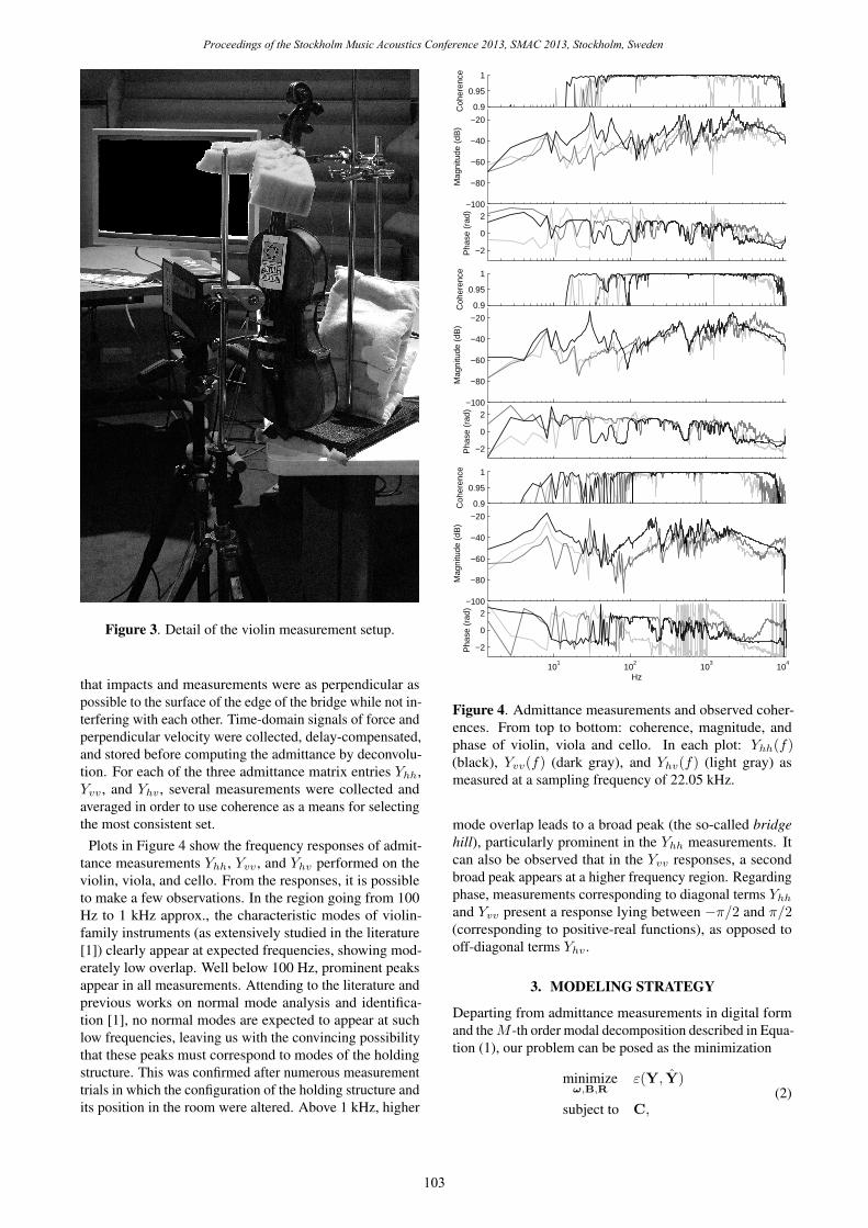
Figure 3. Detail of the violin measurement setup.

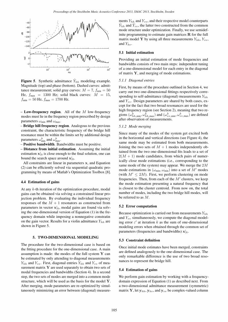
that impacts and measurements were as perpendicular aspossible to the surface of the edge of the bridge while not in-terfering with each other. Time-domain signals of force andperpendicular velocity were collected, delay-compensated,and stored before computing the admittance by deconvolu-tion. For each of the three admittance matrix entries Yhh,Yvv, and Yhv, several measurements were collected andaveraged in order to use coherence as a means for selectingthe most consistent set.

Plots in Figure 4 show the frequency responses of admit-tance measurements Yhh, Yvv, and Yhv performed on theviolin, viola, and cello. From the responses, it is possibleto make a few observations. In the region going from 100Hz to 1 kHz approx., the characteristic modes of violin-family instruments (as extensively studied in the literature[1]) clearly appear at expected frequencies, showing mod-erately low overlap. Well below 100 Hz, prominent peaksappear in all measurements. Attending to the literature andprevious works on normal mode analysis and identifica-tion [1], no normal modes are expected to appear at suchlow frequencies, leaving us with the convincing possibilitythat these peaks must correspond to modes of the holdingstructure. This was confirmed after numerous measurementtrials in which the configuration of the holding structure andits position in the room were altered. Above 1 kHz, higher

0.9

0.95

1

Coh

eren

ce

−100

−80

−60

−40

−20

Mag

nitu

de (

dB)

101

102

103

104

−2

0

2

Pha

se (

rad)

Hz

0.9

0.95

1

Coh

eren

ce

−100

−80

−60

−40

−20

Mag

nitu

de (

dB)

101

102

103

104

−2

0

2

Pha

se (

rad)

Hz

0.9

0.95

1

Coh

eren

ce

−100

−80

−60

−40

−20

Mag

nitu

de (

dB)

101

102

103

104

−2

0

2

Pha

se (

rad)

Hz

Figure 4. Admittance measurements and observed coher-ences. From top to bottom: coherence, magnitude, andphase of violin, viola and cello. In each plot: Yhh(f)(black), Yvv(f) (dark gray), and Yhv(f) (light gray) asmeasured at a sampling frequency of 22.05 kHz.

mode overlap leads to a broad peak (the so-called bridgehill), particularly prominent in the Yhh measurements. Itcan also be observed that in the Yvv responses, a secondbroad peak appears at a higher frequency region. Regardingphase, measurements corresponding to diagonal terms Yhhand Yvv present a response lying between −π/2 and π/2(corresponding to positive-real functions), as opposed tooff-diagonal terms Yhv .

3. MODELING STRATEGY

Departing from admittance measurements in digital formand theM -th order modal decomposition described in Equa-tion (1), our problem can be posed as the minimization

minimizeω,B,R

ε(Y, Y)

subject to C,(2)

Proceedings of the Stockholm Music Acoustics Conference 2013, SMAC 2013, Stockholm, Sweden

103

where ω = {ω1, · · · , ωM} are the modal natural frequen-cies, B = {B1, · · · , BM} are the modal bandwidths, R =

{R1, · · · ,RM} are the gain matrices, ε(Y, Y) is the er-ror between the measured admittance matrix Y and theadmittance model Y, and C is a set of constraints. Thisproblem, for which analytical solution is not available, canbe solved by means of gradient descent methods that makeuse of local (quadratic) approximations of the error functionε(Y, Y). Given the way our fitting problem is posed, fivemain issues need to be taken into consideration:– Design parameters. From observation of each diagonalentry Yhh and Yvv of the measured admittance matrices (seeSection 2), and by contrasting with relevant literature onmodal analysis of violin family instruments [1], we maketwo assumptions. First, at low frequencies (approximatelybetween 100 Hz and 1 kHz) modes of interest present rela-tively low overlap and can be identified and modeled indi-vidually. Second, at higher frequencies (above 1 kHz) highmode overlap leads to a broad peak (bridge hill) that canmodeled by a single, highly-damped resonance. This leavesus with three design parameters: frequencies ωmin and ωmax,and number of low-frequency modes M . Between frequen-cies ωmin and ωmax, M modes are identified and modeledindividually, while above ωmax the bridge hill is modeled bya single mode. When studying the two-dimensional case,we found that using two high-frequency modes provides abetter basis for modeling the bridge hill (see Section 2 andSection 5.1).– Initial estimation. Because the minimization problem,Equation (2) is not convex, it is very important to choose astarting point that is close enough to the global minimum.Therefore, it is crucial to carry out an initial estimation ofmode parameters prior to optimization. The method, tobe described in Section 4.1, is based on peak (resonance)picking from the magnitude spectrum, and a graphical esti-mation of each mode frequency and bandwidth.– Constraint definition. Defining constraints on the param-eters of the problem is motivated by two reasons: feasibilityand convergence. First, a number of feasibility constraintsare needed to obtain a realizable solution. Second, in orderto ensure that the optimization algorithm will not jump intoregions of the parameter space where it can get stuck in lo-cal minima, additional constraints need to be defined so thatcandidate solutions stay within the region of convergence.– Error computation. Since there is no analytical expres-sion for the gradient of this error minimization, it needs tobe estimated from computing the error in different direc-tions around a point in the parameter space. Therefore, weneed to choose a convenient method for computing ε(Y, Y)at any point in the parameter space.– Estimation of gains. Once the M modal frequencies andbandwidths are optimized, it is necessary to perform anestimation of matrices R of Equation (2) to complete themodel of Equation (1).

4. ONE-DIMENSIONAL MODELING

The one-dimensional procedure presented here can be usedboth for Yhh and Yvv. First, once design parameters M ,fmin, and fmax have been set, individual mode resonances

are identified from the magnitude spectrum through a peakpicking iterative procedure. Then, an initial estimation ofmode parameters (frequencies and bandwidths) is obtainedvia the half-power method. In a final step, mode parametersare tuned via numerical optimization.

4.1 Initial estimation

4.1.1 Peak selection

Peak selection in the low-frequency region is carried outthrough an automatic procedure that iteratively rates andsorts spectral peaks by attending to a salience descriptor.The high-frequency bridge hill resonance center frequencyis selected via smoothing the magnitude spectrum.

4.1.2 Estimation of frequencies and bandwidths

For estimating modal frequencies, three magnitude samples(respectively corresponding to the corresponding maximumand its adjacent samples) are used to perform parabolicinterpolation. For estimating bandwidths, the half-powerrule [2] is applied using a linear approximation.

4.2 Error computation

For optimization routines to successfully approximate errorderivatives, it is necessary to supply a procedure to evaluatethe error function as a function of the model parameters,namely a vector x. In our case, parameters are (see Equa-tion 2) mode frequencies ω and bandwidths B. Thus xis constructed by concatenating elements in sets ω and B,leading to x = [ω B]T . We work with frequency-domainrepresentations of the admittance measurement Y and ad-mittance model Y . At the k-th iteration, parameter vector isx|k, and evaluating ε(Y, Y |k) implies: (i) retrieving modefrequencies and bandwidths from x|k, (ii) estimating gainsas outlined in Section 4.4, (iii) constructing a syntheticadmittance Y |k with computed gains, and (iv) computingerror ε(Y, Y |k).Let vector y = [y1, . . . , yn, . . . , yN ]T contain N samplesof Y (ω), taken in 0 ≤ ω < π. Analogously, let y|k =[y1|k, . . . , yn|k, . . . , yN |k]T contain N samples of Y (ω)|k,constructed from parameter vector x|k. We compute theerror ε(Y, Y |k) as

ε(Y, Y |k) =N∑

n=1

∣∣∣log |yn||yn|k|

∣∣∣, (3)

which can be interpreted as subtracting magnitudes whenexpressed in the logarithmic scale.

4.3 Constraint definition

Apart from providing a reliable initial point x|0 (see Section4.1), we need to define a set of constraints to be respectedduring the search:– Mode sequence order. A first important constraint to berespected during the search is the sequence order of modes(in ascending characteristic frequency) as they were initiallyestimated (see Section 4.1).

Proceedings of the Stockholm Music Acoustics Conference 2013, SMAC 2013, Stockholm, Sweden

104

−140

−120

−100

−80

−60

−40dB

101

102

103

104

−2

0

2

rad

Hz

Figure 5. Synthetic admittance Yhh modeling example.Magnitude (top) and phase (bottom). Dashed curves: admit-tance measurement; solid gray curves: M = 7, fmin = 50Hz, fmax = 1300 Hz; solid black curves: M = 15,fmin = 50 Hz, fmax = 1700 Hz.

– Low-frequency region. All of the M low-frequencymodes must lie in the frequency region prescribed by designparameters ωmin and ωmax.– Bridge hill frequency region. Analogous to the previousconstraint, the characteristic frequency of the bridge hillresonance must be within the limits set by additional designparameters ωb

min and ωbmax.

– Positive bandwidth. Bandwidths must be positive.– Distance from initial estimation. Assuming the initialestimation x|0 is close enough to the final solution, one canbound the search space around x|0.

All constraints are linear in parameters x, and Equation(2) can be efficiently solved via sequential quadratic pro-gramming by means of Matlab’s Optimization Toolbox [8].

4.4 Estimation of gains

At any k-th iteration of the optimization procedure, modalgains can be obtained via solving a constrained linear pro-jection problem. By evaluating the individual frequencyresponses of the M + 1 resonators as constructed fromparameters in vector x|k, modal gains are found via solv-ing the one-dimensional version of Equation (1) in the fre-quency domain while imposing a nonnegative constratinon the gain vector. Results for a violin admittance Yhh areshown in Figure 5.

5. TWO-DIMENSIONAL MODELING

The procedure for the two-dimensional case is based onthe fitting procedure for the one-dimensional case. A mainassumption is made: the modes of the full system Y canbe estimated by only attending to diagonal measurementsYhh and Yvv. First, diagonal entries Yhh and Yvv of mea-surement matrix Y are used separately to obtain two sets ofmodal frequencies and bandwidths (Section 4). In a secondstep, the two sets of modes are merged into a common modestructure, which will be used as the basis for the model Y.After merging, mode parameters are re-optimized by simul-taneously minimizing an error between (diagonal) measure-

ments Yhh and Yvv , and their respective model counterpartsYhh and Yvv, the latter two constructed from the commonmode structure under optimization. Finally, we use semidef-inite programming to estimate gain matrices R for the fullmatrix model Y by using all three measurements Yhh, Yvv ,and Yhv .

5.1 Initial estimation

Providing an initial estimation of mode frequencies andbandwidths consists of two main steps: independent tuningof a one-dimensional model for each entry in the diagonalof matrix Y, and merging of mode estimations.

5.1.1 Diagonal entries

First, by means of the procedure outlined in Section 4, wecarry out two one-dimensional fittings respectively corre-sponding to self-admittance (diagonal) measurements Yhhand Yvv. Design parameters are shared by both cases, ex-cept for the fact that two broad resonances are used for thehigh frequency region (see Section 2), meaning that two re-gions (ωb

hh,min, ωbhh,max) and (ωb

vv,min, ωbvv,max) are defined

after observation of measurements.

5.1.2 Mode merging

Since many of the modes of the system get excited bothin the horizontal and vertical directions (see Figure 4), thesame mode may be estimated from both measurements.Joining the two sets of M + 1 modes independently ob-tained from the two one-dimensional fits leads to a set of2(M + 1) mode candidates, from which pairs of numer-ically close mode estimations (i.e., corresponding to thesame mode of the system) may appear. We merge the 2Mmode estimations in (ωmin, ωmin) into a set of M ′ modes(with M ′ ≤ 2M ). First, we perform clustering on modefrequencies. Then, from each of the M ′ clusters, we keepthe mode estimation presenting a natural frequency thatis closest to the cluster centroid. From now on, the totalnumber of modes, including the two bridge hill modes, willbe referred to as M .

5.2 Error computation

Because optimization is carried out from measurements Yhhand Yvv simultaneously, we compute the diagonal model-ing error ε′ at iteration k as the sum of one-dimensionalmodeling errors when obtained through the common set ofparameters (frequencies and bandwidths) x|k.

5.3 Constraint definition

Once initial mode estimates have been merged, constraintsare defined analogously to the one-dimensional case. Theonly remarkable difference is the use of two broad reso-nances to represent the bridge hill.

5.4 Estimation of gains

We perform gain estimation by working with a frequency-domain expression of Equation (1) as described next. Froma two-dimensional admittance measurement (symmetric)matrix Y, let yhh, yhv , and yvv be complex-valued column

Proceedings of the Stockholm Music Acoustics Conference 2013, SMAC 2013, Stockholm, Sweden

105

vectors each containing N frequency-domain samples ofits corresponding entry in Y, leading to a 2N × 2 matrixof the form

Y =

[yhh yhv

yhv yvv

]. (4)

Now, we proceed with rewriting the right-side of Equation(1) in matrix form as constructed from linear combinationsof frequency-domain samples of the individual modal re-sponses Hm(ω). First, we define a N ×M matrix H as

H = [h1, . . .hm . . .hM ], (5)

where each hm is a complex column vector containingN samples of Hm(ω). With matrix H, we construct a2N × 2M block-diagonal matrix B defined as

B =

[H 00 H

], (6)

which can be interpreted as a two-dimensional modal basis.The next step is to set up a 2M × 2M block-symmetricmatrix R as

R =

[Rhh Rhv

Rhv Rvv

], (7)

where Rhh, Rhv , and Rvv are M ×M diagonal, real matri-ces. In them-th entry of the diagonal of matrix Rhh appearsthe gain from entry (1, 1) of the individual gain matrix Rm

in Equation (1). Analogously, matrix Rhv will contain gainsfrom theM entries (1, 2), and Rvv from entries (2, 2). Now,with modal basis B and gain matrix R, it is possible to writean expression for model Y as

Y = BRS, (8)

where S is a 2M × 2 matrix of ones which acts as thesummation of Equation (1). It is important to note thatR � 0 ⇔ Rm � 0 ∀m ∈ {1, . . . ,M}, implying that themodel Y will be passive if matrix R is positive semidefinite.Now we are ready to express the modal gain estimationproblem as an error minimization problem that includes apositive semidefinite constraint on matrix R. If expressingthe model approximation error ε(Y, Y) as

ε(Y, Y) = ‖(Y −Y)‖ = ‖(BRS−Y)‖, (9)

where ‖·‖ represents a suitable matrix norm, the problemcan be written as

minimizeR

‖(BRS−Y)‖

subject to R � 0,(10)

which is a matrix norm minimization problem with a pos-itive semidefinite constraint. This convex problem can besolved via semidefinite programming by means of CVX, apackage for specifying and solving convex programs [9].

−100

−80

−60

−40

−20

dB

101

102

103

104

−2

0

2

Hz

rad

−100

−80

−60

−40

−20

dB10

110

210

310

4

−2

0

2

Hzra

d

−100

−80

−60

−40

−20

dB

101

102

103

104

−2

0

2

Hz

rad

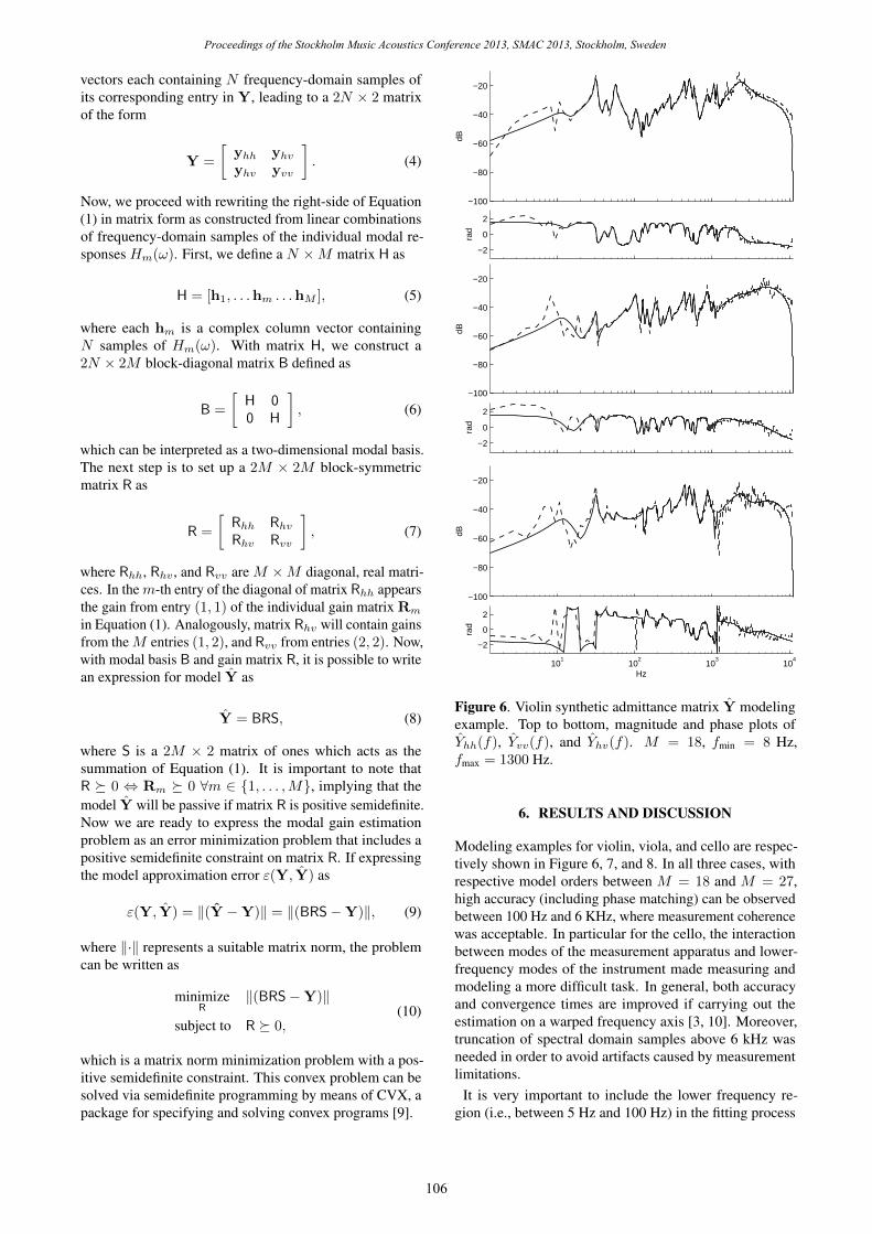
Figure 6. Violin synthetic admittance matrix Y modelingexample. Top to bottom, magnitude and phase plots ofYhh(f), Yvv(f), and Yhv(f). M = 18, fmin = 8 Hz,fmax = 1300 Hz.

6. RESULTS AND DISCUSSION

Modeling examples for violin, viola, and cello are respec-tively shown in Figure 6, 7, and 8. In all three cases, withrespective model orders between M = 18 and M = 27,high accuracy (including phase matching) can be observedbetween 100 Hz and 6 KHz, where measurement coherencewas acceptable. In particular for the cello, the interactionbetween modes of the measurement apparatus and lower-frequency modes of the instrument made measuring andmodeling a more difficult task. In general, both accuracyand convergence times are improved if carrying out theestimation on a warped frequency axis [3, 10]. Moreover,truncation of spectral domain samples above 6 kHz wasneeded in order to avoid artifacts caused by measurementlimitations.

It is very important to include the lower frequency re-gion (i.e., between 5 Hz and 100 Hz) in the fitting process

Proceedings of the Stockholm Music Acoustics Conference 2013, SMAC 2013, Stockholm, Sweden

106

−100

−80

−60

−40

−20dB

101

102

103

104

−2

0

2

Hz

rad

−100

−80

−60

−40

−20

dB

101

102

103

104

−2

0

2

Hz

rad

−100

−80

−60

−40

−20

dB

101

102

103

104

−2

0

2

Hz

rad

Figure 7. Viola synthetic admittance matrix Y modelingexample. Top to bottom, magnitude and phase plots ofYhh(f), Yvv(f), and Yhv(f). M = 22, fmin = 8 Hz,fmax = 1300 Hz.

by setting design parameter ωmin close to dc. This allowsthe modes of the measurement apparatus (prominent peaksbelow 100 Hz) to also be modeled, leading to a more con-sistent overall estimation that accounts for the interactionof such modes with the real modes of the instrument. Oncethe estimation is finished, those modes and their respectivegain matrices can be discarded from Equation (1).

Regarding implementation, an elegant re-formulation ofsecond-order sections proposed in [11] and later appliedin [6] allows to maintain the parallel structure, leading toa straightforward realization as a reflectance. Our resultsfrom applying such re-formulation have been used to con-struct lumped terminations where four two-dimensionaldigital waveguides are coupled without the need for paral-lel adaptors (as in wave digital filters—see [6]). Examplesounds, including one-pole filters to simulate string losses,

−100

−80

−60

−40

−20

dB

101

102

103

104

−2

0

2

Hz

rad

−100

−80

−60

−40

−20

dB

101

102

103

104

−2

0

2

rad

Hz

−100

−80

−60

−40

−20

dB

101

102

103

104

−2

0

2

Hz

rad

Figure 8. Cello synthetic admittance matrix Y modelingexample. Top to bottom, magnitude and phase plots ofYhh(f), Yvv(f), and Yhv(f). M = 27, fmin = 8 Hz,fmax = 900 Hz.

are available online 1 . The application of these models tobowed-string simulation with two-dimensional transversestring motion is imminent.

A potential improvement to the fitting method goes aroundembedding the semidefinite programming step as part ofan outer loop in which mode parameters are estimated,although it would imply a higher computational cost. Byincreasing the model order and redefining design parametersit would be possible to represent the bridge hill region moreaccurately; yet, a perceptual evaluation might be needed toconfirm improvements. Further tests might encourage theconstruction of statistical admittance models, where modalfrequencies, bandwidths, and amplitudes follow empiricallyinferred distributions. An extension of the framework toinclude radiation measurements is currently under study.

1 http://ccrma.stanford.edu/˜esteban/adm/smac13

Proceedings of the Stockholm Music Acoustics Conference 2013, SMAC 2013, Stockholm, Sweden

107

Acknowledgments

This work was partially funded by the Catalan Gov. througha Beatriu de Pinos Fellowship. Thanks go to Argyris Zym-nis and Jonathan S. Abel for inspiring discussions.

7. REFERENCES

[1] T. Rossing, The Science of String Instruments. SpringerNew York, 2010.

[2] J. O. Smith, Physical Audio Signal Processing, Decem-ber 2008 Edition. http://ccrma.stanford.edu/∼jos/pasp/,accessed 2012, online book.

[3] ——, “Techniques for digital filter design and systemidentification with application to the violin,” Ph.D. dis-sertation, Stanford University, 1983.

[4] M. Karjalainen and J. O. Smith, “Body modeling tech-niques for string instrument synthesis,” in Proc. of theInternational Computer Music Conference, 1996.

[5] K. D. Marshall, “Modal analysis of a violin,” Journalof the Acoustical Society of America, vol. 77:2, pp. 695–709, 1985.

[6] B. Bank and M. Karjalainen, “Passive admittance matrixmodeling for guitar synthesis,” in Proc. of the 13th In-ternational Conference on Digital Audio Effects, 2010.

[7] J. M. Adrien, “The missing link: Modal synthesis,” inRepresentations of Musical Signals, G. D. Poli, A. Pic-cialli, and C. Roads, Eds. MIT Press, 1991, pp. 269–267.

[8] MATLAB, version 7.10.0 (R2010a). Natick, Mas-sachusetts: The MathWorks Inc., 2010.

[9] M. Grant and S. Boyd, “CVX: Matlab software fordisciplined convex programming, version 1.21,” http://cvxr.com/cvx/, Apr. 2011.

[10] A. Harma, M. Karjalainen, L. Savioja, V. Valimaki,U. K. Laine, and J. Huopaniemi, “Frequency-warpedsignal processing for audio applications,” Journal of theAudio Engineering Society, vol. 48(11), pp. 1011–1031,2000.

[11] M. Karjalainen, “Efficient realization of wave digitalcomponents for physical modeling and sound synthesis,”IEEE Trans. Audio, Speech, and Lang. Process., vol.16:5, pp. 947–956, 2008.

Proceedings of the Stockholm Music Acoustics Conference 2013, SMAC 2013, Stockholm, Sweden

108