CM0268MATLAB

DSPGRAPHICS

1

332

JJIIJI

Back

Close

Digital Audio EffectsHaving learned to make basic waveforms and basic filtering lets

see how we can add some digital audio effects. These may be applied:

• As part of the audio creation/synthesis stage — to be subsequentlyfiltered, (re)synthesised

• At the end of the audio chain — as part of the production/masteringphase.

• Effects can be applied in different orders and sometimes in aparallel audio chain.

• The order of applying the same effects can have drastic differencesin the output audio.

• Selection of effects and the ordering is a matter for the sound youwish to create. There is no absolute rule for the ordering.

CM0268MATLAB

DSPGRAPHICS

1

333

JJIIJI

Back

Close

Typical Guitar (and other) Effects Pipeline

Some ordering is standard for some audio processing, E.g:Compression→ Distortion→ EQ→ Noise Redux→ Amp Sim→Modulation→ Delay→ Reverb

Common for some guitar effects pedal:

ZOOM G1/G1X18

Compressor

Auto Wah

Booster

Tremolo

Phaser

FD Clean

VX Clean

HW Clean

US Blues

BG Crunch

Hall

Room

Spring

Arena

Tiled Room

Delay

Tape Echo

AnalogDelay

Ping PongDelay

AMP Sim.ZNR Chorus

Ensemble

Flanger

Step

Pitch Shift

COMP/EFX DRIVE EQ MODULATION REVERBDELAYAMPZNREffect modules

Effect types

Effect Types and Parameters

Linking Effects

The patches of the G1/G1X consist of eightserially linked effect modules, as shown in the

illustration below. You can use all effectmodules together or selectively set certainmodules to on or off.

Explanation of symbols

! Module selectorThe Module selector symbolshows the position of the knob atwhich this module/parameter iscalled up.

! Expression pedalA peda l i con in t he l i s t i ngindicates a parameter that can becontrolled with the built-in or anexternal expression pedal.

When this item is selected, the parameter in themodule can then be controlled in real time with aconnected expression pedal.

! TapA [TAP] icon in the l i s t ingindicates a parameter that can beset with the [BANK UP•TAP]key.

When the respective module/effect type isselected in edit mode and the [BANK UP•TAP]key is pressed repeatedly, the parameter (such asmodulation rate or delay time) will be setaccording to the interval in which the key ispressed.

TAP

* Manufacturer names and product names mentioned in this listing are trademarks or registered trademarks of their respective owners. The names are used only to illustrate sonic characteristics and do not indicate any affiliation with ZOOM CORPORATION.

For some effect modules, you can select an effect type from several possible choices. For example, theMODULATION module comprises Chorus, Flanger, and other effect types. The REVERB modulecomprises Hall, Room, and other effect types from which you can choose one.

Effect Types and Parameters

ZOOM G1/G1X 19

"PATCH LEVEL

"COMP/EFX (Compressor/EFX) module

"DRIVE module

PATCH LEVEL (Prm)

Determines the overall volume level of the patch.

Sets the patch level in the range from 2 – 98, 1.0. A setting of 80 corresponds to unity gain (input level and output level are equal).

This module comprises the effects that control the level dynamics such as compressor, and modulation effects such as tremolo and phaser.

COMP/EFX (Type&Prm)

Adjusts the COMP/EFX module effect type and intensity.

CompressorThis is an MXR Dynacomp type compressor. It attenuates high-level signal components and boosts low-level signal components, to keep the overall signal level within a certain range. Higher setting values result in higher sensitivity.

Auto WahThis effect varies wah in accordance with picking intensity. Higher setting values result in higher sensitivity.

BoosterRaises signal level and creates a dynamic sound. Higher setting values result in higher gain.

TremoloThis effect periodically varies the volume. Higher setting values result in faster modulation rate.

PhaserThis effect produces sound with a pulsating character. Higher setting values result in faster modulation rate.

Ring Mod (Ring Modulator)This effect produces a metallic ringing sound. Higher setting values result in higher modulation frequency.

Slow AttackThis effect reduces the attack rate of each individual note, producing a violin playing style sound. Higher setting values result in slower attack times.

Vox WahThis effect simulates a half-open vintage VOX wah pedal. Higher setting values result in higher emphasized frequency.

Cry WahThis effect simulates a half-open vintage Crybaby wah pedal. Higher setting values result in higher emphasized frequency.

This module includes 20 types of distortion and an acoustic simulator. For this module, the two items DRIVE and GAIN can be adjusted separately.

DRIVE (Type)

Selects the effect type for the DRIVE module.

FD Clean VX CleanClean sound of a Fender Twin Reverb ('65 model) favored by guitarists of many music styles.

Clean sound of the combo amp VOX AC-30 operating in class A.

2 10

C1 C9

A1 A9

B1 B9

T1 T9

P1 P9

R1 R9

S1 S9

V1 V9

1 9

FD V

Note: Other Effects Units allow for a completely reconfigurableeffects pipeline. E.g. Boss GT-8

CM0268MATLAB

DSPGRAPHICS

1

334

JJIIJI

Back

Close

Classifying EffectsAudio effects can be classified by the way do their processing:

Basic Filtering — Lowpass, Highpass filter etc,, Equaliser

Time Varying Filters — Wah-wah, Phaser

Delays — Vibrato, Flanger, Chorus, Echo

Modulators — Ring modulation, Tremolo, Vibrato

Non-linear Processing — Compression, Limiters, Distortion,Exciters/Enhancers

Spacial Effects — Panning, Reverb, Surround Sound

CM0268MATLAB

DSPGRAPHICS

1

335

JJIIJI

Back

Close

Basic Digital Audio Filtering Effects:Equalisers

Filters by definition remove/attenuate audio from the spectrumabove or below some cut-off frequency.

• For many audio applications this a little too restrictive

Equalisers, by contrast, enhance/diminish certain frequency bandswhilst leaving others unchanged:

• Built using a series of shelving and peak filters

• First or second-order filters usually employed.

CM0268MATLAB

DSPGRAPHICS

1

336

JJIIJI

Back

Close

Shelving and Peak FiltersShelving Filter — Boost or cut the low or high frequency bands with

a cut-off frequency, Fc and gain G

Peak Filter — Boost or cut mid-frequency bands with a cut-offfrequency, Fc, a bandwidth, fb and gain G

CM0268MATLAB

DSPGRAPHICS

1

337

JJIIJI

Back

Close

Shelving FiltersA first-order shelving filter may be described by the transfer function:

H(z) = 1 +H0

2(1± A(z)) where LF/HF + /−

where A(z) is a first-order allpass filter — passes all frequenciesbut modifies phase:

A(z) =z−1 + aB/C1 + aB/Cz−1

B=Boost, C=Cut

which leads the following algorithm/difference equation:

y1(n) = aB/Cx(n) + x(n− 1)− aB/Cy1(n− 1)

y(n) =H0

2(x(n)± y1(n)) + x(n)

CM0268MATLAB

DSPGRAPHICS

1

338

JJIIJI

Back

Close

Shelving Filters (Cont.)

The gain, G, in dB can be adjusted accordingly:

H0 = V0 − 1 where V0 = 10G/20

and the cut-off frequency for boost, aB, or cut, aC are given by:

aB =tan(2πfc/fs)− 1

tan(2πfc/fs) + 1

aC =tan(2πfc/fs)− V0

tan(2πfc/fs)− V0

CM0268MATLAB

DSPGRAPHICS

1

339

JJIIJI

Back

Close

Shelving Filters Signal Flow Graph

y(n)A(z) ± !H0/2

+x(n) y1(n)

1

where A(z) is given by:T

x(n ! 1)

y(n)

" "aB/C 1

+ +

" !aB/C

T

y1(n ! 1)

x(n)

1

CM0268MATLAB

DSPGRAPHICS

1

340

JJIIJI

Back

Close

Peak FiltersA first-order shelving filter may be described by the transfer function:

H(z) = 1 +H0

2(1− A2(z))

where A2(z) is a second-order allpass filter:

A(z) =−aB + (d− daB)z−1 + z−2

1 + (d− daB)z−1 + aBz−2

which leads the following algorithm/difference equation:

y1(n) = 1aB/Cx(n) + d(1− aB/C)x(n− 1) + x(n− 2)

−d(1− aB/C)y1(n− 1) + aB/Cy1(n− 2)

y(n) =H0

2(x(n)− y1(n)) + x(n)

CM0268MATLAB

DSPGRAPHICS

1

341

JJIIJI

Back

Close

Peak Filters (Cont.)

The center/cut-off frequency, d, is given by:

d = −cos(2πfc/fs)

The H0 by relation to the gain, G, as before:

H0 = V0 − 1 where V0 = 10G/20

and the bandwidth, fb is given by the limits for boost, aB, or cut,aC are given by:

aB =tan(2πfb/fs)− 1

tan(2πfb/fs) + 1

aC =tan(2πfb/fs)− V0

tan(2πfb/fs)− V0

CM0268MATLAB

DSPGRAPHICS

1

342

JJIIJI

Back

Close

Peak Filters Signal Flow Graph

y(n)A(z) +! !"1 H0/2

+x(n) y1(n)

1

where A(z) is given by:x(n)

T T

x(n ! 1) x(n ! 2)

" " "!aB/C d(1 ! aB/C) 1

+ + +y(n)

" "aB/C !d(1 ! aB/C)

T Ty1(n ! 2) y1(n ! 1)

1

CM0268MATLAB

DSPGRAPHICS

1

343

JJIIJI

Back

Close

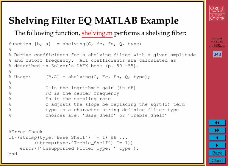
Shelving Filter EQ MATLAB ExampleThe following function, shelving.m performs a shelving filter:

function [b, a] = shelving(G, fc, fs, Q, type)%% Derive coefficients for a shelving filter with a given amplitude% and cutoff frequency. All coefficients are calculated as% described in Zolzer’s DAFX book (p. 50 -55).%% Usage: [B,A] = shelving(G, Fc, Fs, Q, type);%% G is the logrithmic gain (in dB)% FC is the center frequency% Fs is the sampling rate% Q adjusts the slope be replacing the sqrt(2) term% type is a character string defining filter type% Choices are: ’Base_Shelf’ or ’Treble_Shelf’

%Error Checkif((strcmp(type,’Base_Shelf’) ˜= 1) && ...

(strcmp(type,’Treble_Shelf’) ˜= 1))error([’Unsupported Filter Type: ’ type]);

end

CM0268MATLAB

DSPGRAPHICS

1

344

JJIIJI

Back

Close

K = tan((pi * fc)/fs);V0 = 10ˆ(G/20);root2 = 1/Q; %sqrt(2)

%Invert gain if a cutif(V0 < 1)

V0 = 1/V0;end

%%%%%%%%%%%%%%%%%%%%% BASE BOOST%%%%%%%%%%%%%%%%%%%%if(( G > 0 ) & (strcmp(type,’Base_Shelf’)))

b0 = (1 + sqrt(V0)*root2*K + V0*Kˆ2) / (1 + root2*K + Kˆ2);b1 = (2 * (V0*Kˆ2 - 1) ) / (1 + root2*K + Kˆ2);b2 = (1 - sqrt(V0)*root2*K + V0*Kˆ2) / (1 + root2*K + Kˆ2);a1 = (2 * (Kˆ2 - 1) ) / (1 + root2*K + Kˆ2);a2 = (1 - root2*K + Kˆ2) / (1 + root2*K + Kˆ2);

%%%%%%%%%%%%%%%%%%%%% BASE CUT%%%%%%%%%%%%%%%%%%%%elseif (( G < 0 ) & (strcmp(type,’Base_Shelf’)))

b0 = (1 + root2*K + Kˆ2) / (1 + root2*sqrt(V0)*K + V0*Kˆ2);

CM0268MATLAB

DSPGRAPHICS

1

345

JJIIJI

Back

Close

b1 = (2 * (Kˆ2 - 1) ) / (1 + root2*sqrt(V0)*K + V0*Kˆ2);b2 = (1 - root2*K + Kˆ2) / (1 + root2*sqrt(V0)*K + V0*Kˆ2);a1 = (2 * (V0*Kˆ2 - 1) ) / (1 + root2*sqrt(V0)*K + V0*Kˆ2);a2 = (1 - root2*sqrt(V0)*K + V0*Kˆ2) / ...

(1 + root2*sqrt(V0)*K + V0*Kˆ2);

%%%%%%%%%%%%%%%%%%%%% TREBLE BOOST%%%%%%%%%%%%%%%%%%%%elseif (( G > 0 ) & (strcmp(type,’Treble_Shelf’)))

b0 = (V0 + root2*sqrt(V0)*K + Kˆ2) / (1 + root2*K + Kˆ2);b1 = (2 * (Kˆ2 - V0) ) / (1 + root2*K + Kˆ2);b2 = (V0 - root2*sqrt(V0)*K + Kˆ2) / (1 + root2*K + Kˆ2);a1 = (2 * (Kˆ2 - 1) ) / (1 + root2*K + Kˆ2);a2 = (1 - root2*K + Kˆ2) / (1 + root2*K + Kˆ2);

%%%%%%%%%%%%%%%%%%%%% TREBLE CUT%%%%%%%%%%%%%%%%%%%%

elseif (( G < 0 ) & (strcmp(type,’Treble_Shelf’)))

b0 = (1 + root2*K + Kˆ2) / (V0 + root2*sqrt(V0)*K + Kˆ2);b1 = (2 * (Kˆ2 - 1) ) / (V0 + root2*sqrt(V0)*K + Kˆ2);b2 = (1 - root2*K + Kˆ2) / (V0 + root2*sqrt(V0)*K + Kˆ2);a1 = (2 * ((Kˆ2)/V0 - 1) ) / (1 + root2/sqrt(V0)*K ...

CM0268MATLAB

DSPGRAPHICS

1

346

JJIIJI

Back

Close

+ (Kˆ2)/V0);a2 = (1 - root2/sqrt(V0)*K + (Kˆ2)/V0) / ....

(1 + root2/sqrt(V0)*K + (Kˆ2)/V0);

%%%%%%%%%%%%%%%%%%%%% All-Pass%%%%%%%%%%%%%%%%%%%%else

b0 = V0;b1 = 0;b2 = 0;a1 = 0;a2 = 0;

end

%return valuesa = [ 1, a1, a2];b = [ b0, b1, b2];

CM0268MATLAB

DSPGRAPHICS

1

347

JJIIJI

Back

Close

Shelving Filter EQ MATLAB Example (Cont.)

The following script shelving eg.m illustrates how we use the shelvingfilter function to filter:infile = ’acoustic.wav’;

% read in wav sample[ x, Fs, N ] = wavread(infile);

%set Parameters for Shelving Filter% Change these to experiment with filter

G = 4; fcb = 300; Q = 3; type = ’Base_Shelf’;

[b a] = shelving(G, fcb, Fs, Q, type);yb = filter(b,a, x);

% write output wav fileswavwrite(yb, Fs, N, ’out_bassshelf.wav’);

% plot the original and equalised waveformsfigure(1), hold on;plot(yb,’b’);plot(x,’r’);title(’Bass Shelf Filter Equalised Signal’);

CM0268MATLAB

DSPGRAPHICS

1

348

JJIIJI

Back

Close

%Do treble shelf filterfct = 600; type = ’Treble_Shelf’;

[b a] = shelving(G, fct, Fs, Q, type);yt = filter(b,a, x);

% write output wav fileswavwrite(yt, Fs, N, ’out_treblehelf.wav’);

figure(1), hold on;plot(yb,’g’);plot(x,’r’);title(’Treble Shelf Filter Equalised Signal’);

CM0268MATLAB

DSPGRAPHICS

1

349

JJIIJI

Back

Close

Shelving Filter EQ MATLAB Example (Cont.)

The output from the above code is (red plot is original audio):

0 5 10 15

x 104

−1.5

−1

−0.5

0

0.5

1

1.5Bass Shelf Filter Equalised Signal

0 5 10 15

x 104

−1.5

−1

−0.5

0

0.5

1

1.5Treble Shelf Filter Equalised Signal

Click here to hear: original audio, bass shelf filtered audio,treble shelf filtered audio.

CM0268MATLAB

DSPGRAPHICS

1

350

JJIIJI

Back

Close

Time-varying Filters

Some common effects are realised by simply time varying a filterin a couple of different ways:

Wah-wah — A bandpass filter with a time varying centre (resonant)frequency and a small bandwidth. Filtered signal mixed withdirect signal.

Phasing — A notch filter, that can be realised as set of cascading IIRfilters, again mixed with direct signal.

CM0268MATLAB

DSPGRAPHICS

1

351

JJIIJI

Back

Close

Wah-wah ExampleThe signal flow for a wah-wah is as follows:

y(n)+!

!BP

direct-mix

wah-mixTime

Varying

x(n)

1

where BP is a time varying frequency bandpass filter.

• A phaser is similarly implemented with a notch filter replacingthe bandpass filter.

• A variation is the M -fold wah-wah filter where M tap delaybandpass filters spread over the entire spectrum change theircentre frequencies simultaneously.

• A bell effect can be achieved with around a hundred M tapdelays and narrow bandwidth filters

CM0268MATLAB

DSPGRAPHICS

1

352

JJIIJI

Back

Close

Time Varying Filter Implementation:State Variable Filter

In our audio application of time varying filters we now wantindependent control over the cut-off frequency and damping factorof a filter.

(Borrowed from analog electronics) we can implement aState Variable Filter to solve this problem.

• One further advantage is that we can simultaneously get lowpass,bandpass and highpass filter output.

CM0268MATLAB

DSPGRAPHICS

1

353

JJIIJI

Back

Close

The State Variable Filter

+ +

yh(n)

!

F1

+

yb(n)

!

F1

+

yl(n)

T T

!"1 ! Q1

T

T!"1

x(n)

1

where:

x(n) = input signalyl(n) = lowpass signalyb(n) = bandpass signalyh(n) = highpass signal

CM0268MATLAB

DSPGRAPHICS

1

354

JJIIJI

Back

Close

The State Variable Filter AlgorithmThe algorithm difference equations are given by:

yl(n) = F1yb(n) + yl(n− 1)

yb(n) = F1yh(n) + yb(n− 1)

yh(n) = x(n)− yl(n− 1)−Q1yb(n− 1)

with tuning coefficients F1 and Q1 related to the cut-off frequency,fc, and damping, d:

F1 = 2 sin(πfc/fs), and Q1 = 2d

CM0268MATLAB

DSPGRAPHICS

1

355

JJIIJI

Back

Close

MATLAB Wah-wah ImplementationWe simply implement the State Variable Filter with a variable

frequency, fc. The code listing is wah wah.m:% wah_wah.m state variable band pass%% BP filter with narrow pass band, Fc oscillates up and% down the spectrum% Difference equation taken from DAFX chapter 2%% Changing this from a BP to a BR/BS (notch instead of a bandpass) converts% this effect to a phaser%% yl(n) = F1*yb(n) + yl(n-1)% yb(n) = F1*yh(n) + yb(n-1)% yh(n) = x(n) - yl(n-1) - Q1*yb(n-1)%% vary Fc from 500 to 5000 Hz

infile = ’acoustic.wav’;

% read in wav sample[ x, Fs, N ] = wavread(infile);

CM0268MATLAB

DSPGRAPHICS

1

356

JJIIJI

Back

Close

%%%%%%% EFFECT COEFFICIENTS %%%%%%%%%%%%%%%%%%%%%%%%%%%%%%%%%%%%%%%%%%%%%%%%%%%%%%%%%%%%%%%%%%%%%%%%%%%%%%% damping factor% lower the damping factor the smaller the pass banddamp = 0.05;

% min and max centre cutoff frequency of variable bandpass filterminf=500;maxf=3000;

% wah frequency, how many Hz per second are cycled throughFw = 2000;%%%%%%%%%%%%%%%%%%%%%%%%%%%%%%%%%%%%%%%%%%%%%%%%%

% change in centre frequency per sample (Hz)delta = Fw/Fs;

% create triangle wave of centre frequency valuesFc=minf:delta:maxf;while(length(Fc) < length(x) )

Fc= [ Fc (maxf:-delta:minf) ];Fc= [ Fc (minf:delta:maxf) ];

end

% trim tri wave to size of inputFc = Fc(1:length(x));

CM0268MATLAB

DSPGRAPHICS

1

357

JJIIJI

Back

Close

% difference equation coefficients% must be recalculated each time Fc changesF1 = 2*sin((pi*Fc(1))/Fs);% this dictates size of the pass bandsQ1 = 2*damp;

yh=zeros(size(x)); % create emptly out vectorsyb=zeros(size(x));yl=zeros(size(x));

% first sample, to avoid referencing of negative signalsyh(1) = x(1);yb(1) = F1*yh(1);yl(1) = F1*yb(1);

% apply difference equation to the samplefor n=2:length(x),

yh(n) = x(n) - yl(n-1) - Q1*yb(n-1);yb(n) = F1*yh(n) + yb(n-1);yl(n) = F1*yb(n) + yl(n-1);F1 = 2*sin((pi*Fc(n))/Fs);

end

%normalisemaxyb = max(abs(yb));yb = yb/maxyb;

CM0268MATLAB

DSPGRAPHICS

1

358

JJIIJI

Back

Close

% write output wav fileswavwrite(yb, Fs, N, ’out_wah.wav’);

figure(1)hold onplot(x,’r’);plot(yb,’b’);title(’Wah-wah and original Signal’);

CM0268MATLAB

DSPGRAPHICS

1

359

JJIIJI

Back

Close

Wah-wah MATLAB Example (Cont.)

The output from the above code is (red plot is original audio):

0 5 10 15

x 104

−1

−0.8

−0.6

−0.4

−0.2

0

0.2

0.4

0.6

0.8

1Wah−wah and original Signal

Click here to hear: original audio, wah-wah filtered audio.

CM0268MATLAB

DSPGRAPHICS

1

360

JJIIJI

Back

Close

Wah-wah Code ExplainedThree main parts:

• Create a triangle wave to modulate the centre frequency of thebandpass filter.

• Implementation of state variable filter

• Repeated recalculation if centre frequency within the state variablefilter loop.

CM0268MATLAB

DSPGRAPHICS

1

361

JJIIJI

Back

Close

Wah-wah Code Explained (Cont.)

Creation of triangle waveform we have seen previously— seewaveforms.m.

• Slight modification of this code here to allow ’frequency values’(Y-axis amplitude) to vary rather than frequency of the trianglewaveform — here the frequency of the modulator wave isdetermined by wah-wah rate, F w, usually a low frequency:

% min and max centre cutoff frequency of variable bandpass filterminf=500; maxf=3000;% wah frequency, how many Hz per second are cycled throughFw = 2000;

% change in centre frequency per sample (Hz)delta = Fw/Fs;% create triangle wave of centre frequency valuesFc=minf:delta:maxf;while(length(Fc) < length(x) )

Fc= [ Fc (maxf:-delta:minf) ];Fc= [ Fc (minf:delta:maxf) ];

end% trim tri wave to size of inputFc = Fc(1:length(x));

CM0268MATLAB

DSPGRAPHICS

1

362

JJIIJI

Back

Close

Wah-wah Code Explained (Cont.)

Note: As the Wah-wah rate is not likely to be in perfect sync withinput waveform, x, we must trim it to the same length as x.

Modifications to Wah-wah

• Adding Multiple Delays with differing centre frequency filtersbut all modulated by same Fc gives an M-fold wah-wah

• Changing filter to a notch filter gives a phaser

– Notch Filter (or bandreject/bandstop filter (BR/BS)) —attenuate frequencies in a narrow bandwidth (High Q factor)around cut-off frequency, u0

• See Lab worksheet and useful for coursework

CM0268MATLAB

DSPGRAPHICS

1

363

JJIIJI

Back

Close

Bandreject (BR)/Bandpass(BP) Filters

(Sort of) Seen before (Peak Filter). Here we have, BR/BP:

y(n)A2(z) ±

BR = +BP = !

"

1/2

x(n) y1(n)

1

where A2(z) (a second order allpass filter) is given by:x(n)

T T

x(n ! 1) x(n ! 2)

" " "!c d(1 ! c) 1

+ + +y(n)

" "c !d(1 ! c)

T T

y1(n ! 2) y1(n ! 1)

1

CM0268MATLAB

DSPGRAPHICS

1

364

JJIIJI

Back

Close

Bandreject (BR)/Bandpass(BP) Filters (Cont.)

The difference equation is given by:

y1(n) = −cx(n) + d(1− c)x(n− 1) + x(n− 2)

−d(1− c)y1(n− 1) + cy1(n− 2)

y(n) =1

2(x(n)± y1(n))

whered = −cos(2πfc/fs)

c =tan(2πfc/fs)− 1

tan(2πfc/fs) + 1

Bandreject = +Bandpass = −

CM0268MATLAB

DSPGRAPHICS

1

365

JJIIJI

Back

Close

Delay Based EffectsMany useful audio effects can be implemented using a delay

structure:

• Sounds reflected of walls

– In a cave or large room we here an echo and also reverberationtakes place – this is a different effect — see later

– If walls are closer together repeated reflections can appearas parallel boundaries and we hear a modification of soundcolour instead.

• Vibrato, Flanging, Chorus and Echo are examples of delay effects

CM0268MATLAB

DSPGRAPHICS

1

366

JJIIJI

Back

Close

Basic Delay StructureWe build basic delay structures out of some very basic FIR and IIR

filters:

• We use FIR and IIR comb filters

• Combination of FIR and IIR gives the Universal Comb Filter

CM0268MATLAB

DSPGRAPHICS

1

367

JJIIJI

Back

Close

FIR Comb FilterThis simulates a single delay:

• The input signal is delayed by a given time duration, τ .

• The delayed (processed) signal is added to the input signal someamplitude gain, g

• The difference equation is simply:

y(n) = x(n) + gx(n−M) with M = τ/fs

• The transfer function is:

H(z) = 1 + gz−M

CM0268MATLAB

DSPGRAPHICS

1

368

JJIIJI

Back

Close

FIR Comb Filter Signal Flow Diagram

+y(n)

TM

!

!x(n " M)

1

g

x(n)

1

CM0268MATLAB

DSPGRAPHICS

1

369

JJIIJI

Back

Close

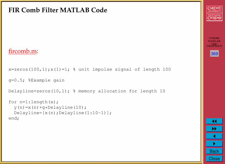
FIR Comb Filter MATLAB Code

fircomb.m:

x=zeros(100,1);x(1)=1; % unit impulse signal of length 100

g=0.5; %Example gain

Delayline=zeros(10,1); % memory allocation for length 10

for n=1:length(x);y(n)=x(n)+g*Delayline(10);Delayline=[x(n);Delayline(1:10-1)];

end;

CM0268MATLAB

DSPGRAPHICS

1

370

JJIIJI

Back

Close

IIR Comb FilterThis simulates a single delay:

• Simulates endless reflections at both ends of cylinder.

• We get an endless series of responses, y(n) to input, x(n).

• The input signal circulates in delay line (delay time τ ) that is fedback to the input..

• Each time it is fed back it is attenuated by g.

• Input sometime scaled by c to compensate for high amplificationof the structure.

• The difference equation is simply:

y(n) = Cx(n) + gy(n−M) with M = τ/fs

• The transfer function is:

H(z) =c

1− gz−M

CM0268MATLAB

DSPGRAPHICS

1

371

JJIIJI

Back

Close

IIR Comb Filter Signal Flow Diagram

! +y(n)

TM

! y(n " M)

g

c

x(n)

1

CM0268MATLAB

DSPGRAPHICS

1

372

JJIIJI

Back

Close

IIR Comb Filter MATLAB Code

iircomb.m:

x=zeros(100,1);x(1)=1; % unit impulse signal of length 100

g=0.5;

Delayline=zeros(10,1); % memory allocation for length 10

for n=1:length(x);y(n)=x(n)+g*Delayline(10);Delayline=[y(n);Delayline(1:10-1)];

end;

CM0268MATLAB

DSPGRAPHICS

1

373

JJIIJI

Back

Close

Universal Comb FilterThe combination of the FIR and IIR comb filters yields the Universal

Comb Filter:

• Basically this is an allpass filter with an M sample delay operatorand an additional multiplier, FF.

TM

x(n ! M)

"

"

BL

FF

+ +y(n)

"FB

x(n)

1

• Parameters: FF = feedforward, FB = feedbackward, BL = blend

CM0268MATLAB

DSPGRAPHICS

1

374

JJIIJI

Back

Close

Universal Comb Filter Parameters

Universal in that we can form any comb filter, an allpass or a delay:

BL FB FFFIR Comb 1 0 gIIR Comb 1 g 0Allpass a −a 1delay 0 0 1

CM0268MATLAB

DSPGRAPHICS

1

375

JJIIJI

Back

Close

Universal Comb Filter MATLAB Code

unicomb.m:

x=zeros(100,1);x(1)=1; % unit impulse signal of length 100

BL=0.5;FB=-0.5;FF=1;M=10;

Delayline=zeros(M,1); % memory allocation for length 10

for n=1:length(x);xh=x(n)+FB*Delayline(M);y(n)=FF*Delayline(M)+BL*xh;Delayline=[xh;Delayline(1:M-1)];

end;

CM0268MATLAB

DSPGRAPHICS

1

376

JJIIJI

Back

Close

Vibrato - A Simple Delay Based Effect• Vibrato — Varying the time delay periodically

• If we vary the distance between and observer and a sound source(cf. Doppler effect) we here a change in pitch.

• Implementation: A Delay line and a low frequency oscillator (LFO)to vary the delay.

• Only listen to the delay — no forward or backward feed.

• Typical delay time = 5–10 Ms and LFO rate 5–14Hz.

CM0268MATLAB

DSPGRAPHICS

1

377

JJIIJI

Back

Close

Vibrato MATLAB Code

vibrato.m function, Use vibrato eg.m to call function:

function y=vibrato(x,SAMPLERATE,Modfreq,Width)

ya_alt=0;Delay=Width; % basic delay of input sample in secDELAY=round(Delay*SAMPLERATE); % basic delay in # samplesWIDTH=round(Width*SAMPLERATE); % modulation width in # samplesif WIDTH>DELAY

error(’delay greater than basic delay !!!’);return;

end;

MODFREQ=Modfreq/SAMPLERATE; % modulation frequency in # samplesLEN=length(x); % # of samples in WAV-fileL=2+DELAY+WIDTH*2; % length of the entire delayDelayline=zeros(L,1); % memory allocation for delayy=zeros(size(x)); % memory allocation for output vector

CM0268MATLAB

DSPGRAPHICS

1

378

JJIIJI

Back

Close

for n=1:(LEN-1)M=MODFREQ;MOD=sin(M*2*pi*n);ZEIGER=1+DELAY+WIDTH*MOD;i=floor(ZEIGER);frac=ZEIGER-i;Delayline=[x(n);Delayline(1:L-1)];%---Linear Interpolation-----------------------------y(n,1)=Delayline(i+1)*frac+Delayline(i)*(1-frac);%---Allpass Interpolation------------------------------%y(n,1)=(Delayline(i+1)+(1-frac)*Delayline(i)-(1-frac)*ya_alt);%ya_alt=ya(n,1);

end

CM0268MATLAB

DSPGRAPHICS

1

379

JJIIJI

Back

Close

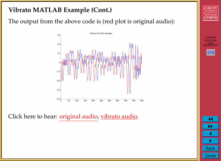
Vibrato MATLAB Example (Cont.)

The output from the above code is (red plot is original audio):

0 50 100 150 200 250 300 350 400 450 500−0.4

−0.3

−0.2

−0.1

0

0.1

0.2

0.3Vibrato First 500 Samples

Click here to hear: original audio, vibrato audio.

CM0268MATLAB

DSPGRAPHICS

1

380

JJIIJI

Back

Close

Vibrato MATLAB Code Explained

Click here to hear: original audio, vibrato audio.The code should be relatively self explanatory, except for one part:

• We work out the delay (modulated by a sinusoid) at each step, n:

M=MODFREQ;MOD=sin(M*2*pi*n);ZEIGER=1+DELAY+WIDTH*MOD;

• We then work out the nearest sample step: i=floor(ZEIGER);

• The problem is that we have a fractional delay line value: ZEIGER

ZEIGER = 11.2779i = 11

ZEIGER = 11.9339i = 11

ZEIGER = 12.2829i = 12

CM0268MATLAB

DSPGRAPHICS

1

381

JJIIJI

Back

Close

Fractional Delay Line - Interpolation

• To improve effect we can use some form of interpolation tocompute the output, y(n).

– Above uses Linear Interpolationy(n,1)=Delayline(i+1)*frac+Delayline(i)*(1-frac);

or:

y(n) = x(n− (M + 1)).frac + x(n−M).(1− frac)– Alternatives (commented in code)

%---Allpass Interpolation------------------------------%y(n,1)=(Delayline(i+1)+(1-frac)*Delayline(i)-...

(1-frac)*ya_alt);%ya_alt=y(n,1);

or:

y(n) = x(n− (M + 1)).frac + x(n−M).(1− frac)−y(n− 1).(1− frac)

– or spline based interpolation — see DAFX book p68-69.

CM0268MATLAB

DSPGRAPHICS

1

382

JJIIJI

Back

Close

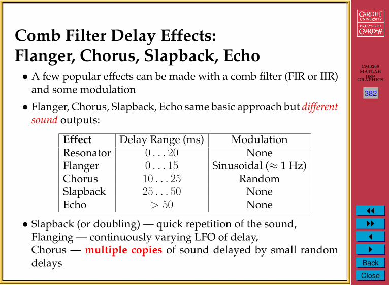
Comb Filter Delay Effects:Flanger, Chorus, Slapback, Echo• A few popular effects can be made with a comb filter (FIR or IIR)

and some modulation

• Flanger, Chorus, Slapback, Echo same basic approach but differentsound outputs:

Effect Delay Range (ms) ModulationResonator 0 . . . 20 NoneFlanger 0 . . . 15 Sinusoidal (≈ 1 Hz)Chorus 10 . . . 25 RandomSlapback 25 . . . 50 NoneEcho > 50 None

• Slapback (or doubling) — quick repetition of the sound,Flanging — continuously varying LFO of delay,Chorus — multiple copies of sound delayed by small randomdelays

CM0268MATLAB

DSPGRAPHICS

1

383

JJIIJI

Back

Close

Flanger MATLAB Code

flanger.m:

% Creates a single FIR delay with the delay time oscillating from% Either 0-3 ms or 0-15 ms at 0.1 - 5 Hz

infile=’acoustic.wav’;outfile=’out_flanger.wav’;

% read the sample waveform[x,Fs,bits] = wavread(infile);

% parameters to vary the effect %max_time_delay=0.003; % 3ms max delay in secondsrate=1; %rate of flange in Hz

index=1:length(x);

% sin reference to create oscillating delaysin_ref = (sin(2*pi*index*(rate/Fs)))’;

%convert delay in ms to max delay in samplesmax_samp_delay=round(max_time_delay*Fs);

% create empty out vectory = zeros(length(x),1);

CM0268MATLAB

DSPGRAPHICS

1

384

JJIIJI

Back

Close

% to avoid referencing of negative samplesy(1:max_samp_delay)=x(1:max_samp_delay);

% set amp suggested coefficient from page 71 DAFXamp=0.7;

% for each samplefor i = (max_samp_delay+1):length(x),cur_sin=abs(sin_ref(i)); %abs of current sin val 0-1% generate delay from 1-max_samp_delay and ensure whole numbercur_delay=ceil(cur_sin*max_samp_delay);% add delayed sampley(i) = (amp*x(i)) + amp*(x(i-cur_delay));

end

% write outputwavwrite(y,Fs,outfile);

CM0268MATLAB

DSPGRAPHICS

1

385

JJIIJI

Back

Close

Flanger MATLAB Example (Cont.)

The output from the above code is (red plot is original audio):

0 5 10 15

x 104

−1.5

−1

−0.5

0

0.5

1

1.5Flanger and original Signal

Click here to hear: original audio, flanged audio.

CM0268MATLAB

DSPGRAPHICS

1

386

JJIIJI

Back

Close

ModulationModulation is the process where parameters of a sinusoidal signal

(amplitude, frequency and phase) are modified or varied by an audiosignal.

We have met some example effects that could be considered as aclass of modulation already:

Amplitude Modulation — Wah-wah, Phaser

Phase Modulation — Vibrato, Chorus, Flanger

We will now introduce some Modulation effects.

CM0268MATLAB

DSPGRAPHICS

1

387

JJIIJI

Back

Close

Ring ModulationRing modulation (RM) is where the audio modulator signal, x(n)

is multiplied by a sine wave, m(n), with a carrier frequency, fc.

• This is very simple to implement digitally:

y(n) = x(n).m(n)

• Although audible result is easy to comprehend for simple signalsthings get more complicated for signals having numerous partials

• If the modulator is also a sine wave with frequency, fx then onehears the sum and difference frequencies: fc+ fx and fc− fx, forexample.

• When the input is periodic with at a fundamental frequency, f0,then a spectrum with amplitude lines at frequencies |kf0 ± fc|• Used to create robotic speech effects on old sci-fi movies and can

create some odd almost non-musical effects if not used with care.(Original speech )

CM0268MATLAB

DSPGRAPHICS

1

388

JJIIJI

Back

Close

MATLAB Ring ModulationTwo examples, a sine wave and an audio sample being modulated

by a sine wave, ring mod.m

filename=’acoustic.wav’;

% read the sample waveform[x,Fs,bits] = wavread(filename);

index = 1:length(x);

% Ring Modulate with a sine wave frequency FcFc = 440;carrier= sin(2*pi*index*(Fc/Fs))’;

% Do Ring Modulationy = x.*carrier;

% write outputwavwrite(y,Fs,bits,’out_ringmod.wav’);

Click here to hear: original audio, ring modulated audio.

CM0268MATLAB

DSPGRAPHICS

1

389

JJIIJI

Back

Close

MATLAB Ring Modulation: Two sine waves% Ring Modulate with a sine wave frequency FcFc = 440;carrier= sin(2*pi*index*(Fc/Fs))’;

%create a modulator sine wave frequency FxFx = 200;modulator = sin(2*pi*index*(Fx/Fs))’;

% Ring Modulate with sine wave, freq. Fcy = modulator.*carrier;

% write outputwavwrite(y,Fs,bits,’twosine_ringmod.wav’);

Output of Two sine wave ring modulation (fc = 440, fx = 380)

0 50 100 150 200 250−1

−0.8

−0.6

−0.4

−0.2

0

0.2

0.4

0.6

0.8

1

Click here to hear: Two RM sine waves (fc = 440, fx = 200)

CM0268MATLAB

DSPGRAPHICS

1

390

JJIIJI

Back

Close

Amplitude ModulationAmplitude Modulation (AM) is defined by:

y(n) = (1 + αm(n)).x(n)

• Normalise the peak amplitude of M(n) to 1.

• α is depth of modulation

α = 1 gives maximum modulationα = 0 tuns off modulation

• x(n) is the audio carrier signal

• m(n) is a low-frequency oscillator modulator.

• When x(n) and m(n) both sine waves with frequencies fc andfx respectively we here three frequencies: carrier, difference andsum: fc, fc − fx, fc + fx.

CM0268MATLAB

DSPGRAPHICS

1

391

JJIIJI

Back

Close

Amplitude Modulation: TremoloA common audio application of AM is to produce a tremolo effect:

• Set modulation frequency of the sine wave to below 20Hz

The MATLAB code to achieve this is tremolo1.m

% read the sample waveformfilename=’acoustic.wav’;[x,Fs,bits] = wavread(filename);

index = 1:length(x);

Fc = 5;alpha = 0.5;

trem=(1+ alpha*sin(2*pi*index*(Fc/Fs)))’;y = trem.*x;

% write outputwavwrite(y,Fs,bits,’out_tremolo1.wav’);

Click here to hear: original audio, AM tremolo audio.

CM0268MATLAB

DSPGRAPHICS

1

392

JJIIJI

Back

Close

Tremolo via Ring Modulation

If you ring modulate with a triangular wave (or try another waveform)you can get tremolo via RM, tremolo2.m% read the sample waveformfilename=’acoustic.wav’;[x,Fs,bits] = wavread(filename);

% create triangular wave LFOdelta=5e-4;minf=-0.5;maxf=0.5;

trem=minf:delta:maxf;while(length(trem) < length(x) )

trem=[trem (maxf:-delta:minf)];trem=[trem (minf:delta:maxf)];

end

%trim tremtrem = trem(1:length(x))’;

%Ring mod with triangular, tremy= x.*trem;

% write outputwavwrite(y,Fs,bits,’out_tremolo2.wav’);

Click here to hear: original audio, RM tremolo audio.

CM0268MATLAB

DSPGRAPHICS

1

393

JJIIJI

Back

Close

Non-linear Processing

Non-linear Processors are characterised by the fact that they create(intentional or unintentional) harmonic and inharmonic frequencycomponents not present in the original signal.

Three major categories of non-linear processing:

Dynamic Processing: control of signal envelop — aim to minimiseharmonic distortion Examples: Compressors, Limiters

Intentional non-linear harmonic processing: Aim to introducestrong harmonic distortion. Examples: Many electric guitar effectssuch as distortion

Exciters/Enhancers: add additional harmonics for subtle soundimprovement.

CM0268MATLAB

DSPGRAPHICS

1

394

JJIIJI

Back

Close

LimiterA Limiter is a device that controls high peaks in a signal but aims

to change the dynamics of the main signal as little as possible:

• A limiter makes use of a peak level measurement and aims toreact very quickly to scale the level if it is above some threshold.

• By lowering peaks the overall signal can be boosted.

• Limiting used not only on single instrument but on final(multichannel) audio for CD mastering, radio broadcast etc.

CM0268MATLAB

DSPGRAPHICS

1

395

JJIIJI

Back

Close

MATLAB Limiter ExampleThe following code creates a modulated sine wave and then limits

the amplitude when it exceeds some threshold,The MATLAB codeto achieve this is limiter.m:

%Create a sine wave with amplitude% reduced for half its duration

anzahl=220;for n=1:anzahl,

x(n)=0.2*sin(n/5);end;for n=anzahl+1:2*anzahl;

x(n)=sin(n/5);end;

CM0268MATLAB

DSPGRAPHICS

1

396

JJIIJI

Back

Close

MATLAB Limiter Example (Cont.)% do Limiter

slope=1;tresh=0.5;rt=0.01;at=0.4;

xd(1)=0; % Records Peaks in xfor n=2:2*anzahl;a=abs(x(n))-xd(n-1);if a<0, a=0; end;

xd(n)=xd(n-1)*(1-rt)+at*a;if xd(n)>tresh,

f(n)=10ˆ(-slope*(log10(xd(n))-log10(tresh)));% linear calculation of f=10ˆ(-LS*(X-LT))

else f(n)=1;end;y(n)=x(n)*f(n);

end;

CM0268MATLAB

DSPGRAPHICS

1

397

JJIIJI

Back

Close

MATLAB Limiter Example (Cont.)

Display of the signals from the above limiter example:

0 50 100 150 200 250 300 350 400 450−1

−0.8

−0.6

−0.4

−0.2

0

0.2

0.4

0.6

0.8

1Input Signal x(n)

0 50 100 150 200 250 300 350 400 450−0.6

−0.4

−0.2

0

0.2

0.4

0.6

0.8Output Signal y(n)

0 50 100 150 200 250 300 350 400 4500

0.1

0.2

0.3

0.4

0.5

0.6

0.7

0.8

0.9

1Input Peak Signal xd(n)

0 50 100 150 200 250 300 350 400 4500

0.1

0.2

0.3

0.4

0.5

0.6

0.7

0.8

0.9

1Gain Signal f(n)

CM0268MATLAB

DSPGRAPHICS

1

398

JJIIJI

Back

Close

Compressors/Expanders

Compressors are used to reduce the dynamics of the input signal:

• Quiet parts are modified

• Loud parts with are reduced according to some static curve.

• A bit like a limiter and uses again to boost overall signals inmastering or other applications.

• Used on vocals and guitar effects.

Expanders operate on low signal levels and boost the dynamics isthese signals.

• Used to create a more lively sound characteristic

CM0268MATLAB

DSPGRAPHICS

1

399

JJIIJI

Back

Close

MATLAB Compressor/ExpanderA MATLAB function for Compression/Expansion, compexp.m:

function y=compexp(x,comp,release,attack,a,Fs)% Compressor/expander% comp - compression: 0>comp>-1, expansion: 0<comp<1% a - filter parameter <1h=filter([(1-a)ˆ2],[1.0000 -2*a aˆ2],abs(x));h=h/max(h);h=h.ˆcomp;y=x.*h;y=y*max(abs(x))/max(abs(y));

CM0268MATLAB

DSPGRAPHICS

1

400

JJIIJI

Back

Close

MATLAB Compressor/Expander (Cont.)

A compressed signal looks like this , compression eg.m:

% read the sample waveformfilename=’acoustic.wav’;[x,Fs,bits] = wavread(filename);

comp = -0.5; %set compressora = 0.5;y = compexp(x,comp,a,Fs);

% write outputwavwrite(y,Fs,bits,...

’out_compression.wav’);

figure(1);hold onplot(y,’r’);plot(x,’b’);title(’Compressed and Boosted Signal’); 0 5 10 15

x 104

−1

−0.8

−0.6

−0.4

−0.2

0

0.2

0.4

0.6

0.8

1Compressed and Boosted Signal

Click here to hear: original audio, compressed audio.

CM0268MATLAB

DSPGRAPHICS

1

401

JJIIJI

Back

Close

MATLAB Compressor/Expander (Cont.)

An expanded signal looks like this , expander eg.m:

% read the sample waveformfilename=’acoustic.wav’;[x,Fs,bits] = wavread(filename);

comp = 0.5; %set expandera = 0.5;y = compexp(x,comp,a,Fs);

% write outputwavwrite(y,Fs,bits,...

’out_compression.wav’);

figure(1);hold onplot(y,’r’);plot(x,’b’);title(’Expander Signal’); 0 5 10 15

x 104

−1

−0.8

−0.6

−0.4

−0.2

0

0.2

0.4

0.6

0.8

1Expander Signal

Click here to hear: original audio, expander audio.

CM0268MATLAB

DSPGRAPHICS

1

402

JJIIJI

Back

Close

Overdrive, Distortion and FuzzDistortion plays an important part in electric guitar music, especially

rock music and its variants.Distortion can be applied as an effect to other instruments includingvocals.

Overdrive — Audio at a low input level is driven by higher inputlevels in a non-linear curve characteristic

Distortion — a wider tonal area than overdrive operating at a highernon-linear region of a curve

Fuzz — complete non-linear behaviour, harder/harsher thandistortion

CM0268MATLAB

DSPGRAPHICS

1

403

JJIIJI

Back

Close

OverdriveFor overdrive, Symmetrical soft clipping of input values has to

be performed. A simple three layer non-linear soft saturation schememay be:

f (x) =

2x for 0 ≤ x < 1/33−(2−3x)2

3for 1/3 ≤ x < 2/3

1 for 2/3 ≤ x ≤ 1

• In the lower third the output is liner — multiplied by 2.

• In the middle third there is a non-linear (quadratic) outputresponse

• Above 2/3 the output is set to 1.

CM0268MATLAB

DSPGRAPHICS

1

404

JJIIJI

Back

Close

MATLAB Overdrive Example

The MATLAB code to perform symmetrical soft clipping is,symclip.m:

function y=symclip(x)% y=symclip(x)% "Overdrive" simulation with symmetrical clipping% x - inputN=length(x);y=zeros(1,N); % Preallocate yth=1/3; % threshold for symmetrical soft clipping

% by Schetzen Formulafor i=1:1:N,

if abs(x(i))< th, y(i)=2*x(i);end;if abs(x(i))>=th,

if x(i)> 0, y(i)=(3-(2-x(i)*3).ˆ2)/3; end;if x(i)< 0, y(i)=-(3-(2-abs(x(i))*3).ˆ2)/3; end;

end;if abs(x(i))>2*th,

if x(i)> 0, y(i)=1;end;if x(i)< 0, y(i)=-1;end;

end;end;

CM0268MATLAB

DSPGRAPHICS

1

405

JJIIJI

Back

Close

MATLAB Overdrive Example (Cont.)

An overdriven signal looks like this , overdrive eg.m:

% read the sample waveformfilename=’acoustic.wav’;[x,Fs,bits] = wavread(filename);

% call symmetrical soft clipping% functiony = symclip(x);

% write outputwavwrite(y,Fs,bits,...

’out_overdrive.wav’);

figure(1);hold onplot(y,’r’);plot(x,’b’);title(’Overdriven Signal’); 0 5 10 15

x 104

−1

−0.8

−0.6

−0.4

−0.2

0

0.2

0.4

0.6

0.8

1Overdriven Signal

Click here to hear: original audio, overdriven audio.

CM0268MATLAB

DSPGRAPHICS

1

406

JJIIJI

Back

Close

Distortion/FuzzA non-linear function commonly used to simulate distortion/fuzz

is given by:

f (x) =x

|x|(1− eαx2/|x|)

• This a non-linear exponential function:

• The gain, α, controls level of distortion/fuzz.

• Common to mix part of the distorted signal with original signalfor output.

CM0268MATLAB

DSPGRAPHICS

1

407

JJIIJI

Back

Close

MATLAB Fuzz Example

The MATLAB code to perform non-linear gain is,fuzzexp.m:

function y=fuzzexp(x, gain, mix)% y=fuzzexp(x, gain, mix)% Distortion based on an exponential function% x - input% gain - amount of distortion, >0->% mix - mix of original and distorted sound, 1=only distortedq=x*gain/max(abs(x));z=sign(-q).*(1-exp(sign(-q).*q));y=mix*z*max(abs(x))/max(abs(z))+(1-mix)*x;y=y*max(abs(x))/max(abs(y));

Note: function allows to mix input and fuzz signals at output

CM0268MATLAB

DSPGRAPHICS

1

408

JJIIJI

Back

Close

MATLAB Fuzz Example (Cont.)

An fuzzed up signal looks like this , fuzz eg.m:

filename=’acoustic.wav’;

% read the sample waveform[x,Fs,bits] = wavread(filename);

% Call fuzzexpgain = 11; % Spinal Tap itmix = 1; % Hear only fuzzy = fuzzexp(x,gain,mix);

% write outputwavwrite(y,Fs,bits,’out_fuzz.wav’);

0 5 10 15

x 104

−1

−0.8

−0.6

−0.4

−0.2

0

0.2

0.4

0.6

0.8

1Fuzz Signal

Click here to hear: original audio, Fuzz audio.

CM0268MATLAB

DSPGRAPHICS

1

409

JJIIJI

Back

Close

Reverb/Spatial EffectsThe final set of effects we look at are effects that change to spatial

localisation of sound. There a many examples of this type of processingwe will study two briefly:

Panning in stereo audio

Reverb — a small selection of reverb algorithms

CM0268MATLAB

DSPGRAPHICS

1

410

JJIIJI

Back

Close

PanningThe simple problem we address here is mapping a monophonic

sound source across a stereo audio image such that the sound startsin one speaker (R) and is moved to the other speaker (L) in n timesteps.• We assume that we listening in a central position so that the angle

between two speakers is the same, i.e. we subtend an angle 2θlbetween 2 speakers. We assume for simplicity, in this case thatθl = 45◦

CM0268MATLAB

DSPGRAPHICS

1

411

JJIIJI

Back

Close

Panning Geometry• We seek to obtain to signals one for each Left (L) and Right (R)

channel, the gains of which, gL and gR, are applied to steer thesound across the stereo audio image.

• This can be achieved by simple 2D rotation, where the angle wesweep is θ:

Aθ =

[cos θ sin θ− sin θ cos θ

]and [

gLgR

]= Aθ.x

where x is a segment of mono audio

CM0268MATLAB

DSPGRAPHICS

1

412

JJIIJI

Back

Close

MATLAB Panning ExampleThe MATLAB code to do panning, matpan.m:

% read the sample waveformfilename=’acoustic.wav’;[monox,Fs,bits] = wavread(filename);

initial_angle = -40; %in degreesfinal_angle = 40; %in degreessegments = 32;angle_increment = (initial_angle - final_angle)/segments * pi / 180;

% in radianslenseg = floor(length(monox)/segments) - 1;pointer = 1;angle = initial_angle * pi / 180; %in radians

y=[[];[]];

for i=1:segmentsA =[cos(angle), sin(angle); -sin(angle), cos(angle)];stereox = [monox(pointer:pointer+lenseg)’; monox(pointer:pointer+lenseg)’];y = [y, A * stereox];angle = angle + angle_increment; pointer = pointer + lenseg;

end;

% write outputwavwrite(y’,Fs,bits,’out_stereopan.wav’);

CM0268MATLAB

DSPGRAPHICS

1

413

JJIIJI

Back

Close

MATLAB Panning Example (Cont.)

0 5 10 15

x 104

−1.5

−1

−0.5

0

0.5

1

1.5Stereo Panned Signal Channel 1 (L)

0 5 10 15

x 104

−1.5

−1

−0.5

0

0.5

1

1.5Stereo Panned Signal Channel 2 (R)

Click here to hear: original audio, stereo panned audio.

CM0268MATLAB

DSPGRAPHICS

1

414

JJIIJI

Back

Close

ReverbReverberation (reverb for short) is probably one of the most heavily

used effects in music.Reverberation is the result of the many reflections of a sound that

occur in a room.

• From any sound source, say a speaker of your stereo, there is adirect path that the sounds covers to reach our ears.

• Sound waves can also take a slightly longer path by reflecting offa wall or the ceiling, before arriving at your ears.

CM0268MATLAB

DSPGRAPHICS

1

415

JJIIJI

Back

Close

The Spaciousness of a Room

• A reflected sound wave like this will arrive a little later than thedirect sound, since it travels a longer distance, and is generallya little weaker, as the walls and other surfaces in the room willabsorb some of the sound energy.

• Reflected waves can again bounce off another wall before arrivingat your ears, and so on.

• This series of delayed and attenuated sound waves is what wecall reverb, and this is what creates the spaciousness sound of aroom.

• Clearly large rooms such as concert halls/cathedrals will have amuch more spaciousness reverb than a living room or bathroom.

CM0268MATLAB

DSPGRAPHICS

1

416

JJIIJI

Back

Close

Reverb v. EchoIs reverb just a series of echoes?

Echo — implies a distinct, delayed version of a sound,

• E.g. as you would hear with a delay more than one ortwo-tenths of a second.

Reverb — each delayed sound wave arrives in such a short periodof time that we do not perceive each reflection as a copy of theoriginal sound.

• Even though we can’t discern every reflection, we still hearthe effect that the entire series of reflections has.

CM0268MATLAB

DSPGRAPHICS

1

417

JJIIJI

Back

Close

Reverb v. Delay

Can a simple delay device with feedback produce reverberation?

Delay can produce a similar effect but there is one very importantfeature that a simple delay unit will not produce:

• The rate of arriving reflections changes over time• Delay can only simulate reflections with a fixed time interval.

Reverb — for a short period after the direct sound, there is generallya set of well defined directional reflections that are directly relatedto the shape and size of the room, and the position of the sourceand listener in the room.

• These are the early reflections• After the early reflections, the rate of the arriving reflections

increases greatly are more random and difficult to relate to thephysical characteristics of the room.This is called the diffuse reverberation, or the late reflections.• Diffuse reverberation is the primary factor establishing a room’s

’spaciousness’ — it decays exponentially in good concert halls.

CM0268MATLAB

DSPGRAPHICS

1

418

JJIIJI

Back

Close

Reverb SimulationsThere are many ways to simulate reverb.

We will only study two classes of approach here (there are others):

• Filter Bank/Delay Line methods

• Convolution/Impulse Response methods

CM0268MATLAB

DSPGRAPHICS

1

419

JJIIJI

Back

Close

Schroeder’s Reverberator• Early digital reverberation algorithms tried to mimic the a rooms

reverberation by primarily using two types of infinite impulseresponse (IIR) filters.

Comb filter — usually in parallel banksAllpass filter — usually sequentially after comb filter banks

• A delay is (set via the feedback loops allpass filter) aims to makethe output would gradually decay.

CM0268MATLAB

DSPGRAPHICS

1

420

JJIIJI

Back

Close

Schroeder’s Reverberator (Cont.)

An example of one of Schroeder’s well-known reverberator designsuses four comb filters and two allpass filters:

Note:This design does not create the increasing arrival rate ofreflections, and is rather primitive when compared to currentalgorithms.

CM0268MATLAB

DSPGRAPHICS

1

421

JJIIJI

Back

Close

MATLAB Schroeder ReverbThe MATLAB function to do Schroeder Reverb, schroeder1.m:

function [y,b,a]=schroeder1(x,n,g,d,k)%This is a reverberator based on Schroeder’s design which consists of n all%pass filters in series.%%The structure is: [y,b,a] = schroeder1(x,n,g,d,k)%%where x = the input signal% n = the number of allpass filters% g = the gain of the allpass filters (should be less than 1 for stability)% d = a vector which contains the delay length of each allpass filter% k = the gain factor of the direct signal% y = the output signal% b = the numerator coefficients of the transfer function% a = the denominator coefficients of the transfer function%% note: Make sure that d is the same length as n.%

% send the input signal through the first allpass filter[y,b,a] = allpass(x,g,d(1));

% send the output of each allpass filter to the input of the next allpass filterfor i = 2:n,

[y,b1,a1] = allpass(y,g,d(i));[b,a] = seriescoefficients(b1,a1,b,a);

end

CM0268MATLAB

DSPGRAPHICS

1

422

JJIIJI

Back

Close

% add the scaled direct signaly = y + k*x;

% normalize the output signaly = y/max(y);

The support files to do the filtering (for following reverb methodsalso) are here:

• delay.m,

• seriescoefficients.m,

• parallelcoefficients.m,

• fbcomb.m,

• ffcomb.m,

• allpass.m

CM0268MATLAB

DSPGRAPHICS

1

423

JJIIJI

Back

Close

MATLAB Schroeder Reverb (Cont.)

An example script to call the function is as follows,reverb schroeder eg.m:

% reverb_Schroeder1_eg.m% Script to call the Schroeder1 Reverb Algoritm

% read the sample waveformfilename=’../acoustic.wav’;[x,Fs,bits] = wavread(filename);

% Call Schroeder1 reverb%set the number of allpass filtersn = 6;%set the gain of the allpass filtersg = 0.9;%set delay of each allpass filter in number of samples%Compute a random set of milliseconds and use sample raterand(’state’,sum(100*clock))d = floor(0.05*rand([1,n])*Fs);%set gain of direct signalk= 0.2;

[y b a] = schroeder1(x,n,g,d,k);

% write outputwavwrite(y,Fs,bits,’out_schroederreverb.wav’);

CM0268MATLAB

DSPGRAPHICS

1

424

JJIIJI

Back

Close

MATLAB Schroeder Reverb (Cont.)

The input signal (blue) and reverberated signal (red) look like this:

0 5 10 15

x 104

−1.5

−1

−0.5

0

0.5

1Schroeder Reverberated Signal

Click here to hear: original audio, Schroeder reverberated audio.

CM0268MATLAB

DSPGRAPHICS

1

425

JJIIJI

Back

Close

MATLAB Schroeder Reverb (Cont.)

The MATLAB function to do the more classic 4 comb and 2 allpassfilter Schroeder Reverb, schroeder2.m:function [y,b,a]=schroeder2(x,cg,cd,ag,ad,k)%This is a reverberator based on Schroeder’s design which consists of 4% parallel feedback comb filters in series with 2 cascaded all pass filters.%%The structure is: [y,b,a] = schroeder2(x,cg,cd,ag,ad,k)%%where x = the input signal% cg = a vector of length 4 which contains the gain of each of the% comb filters (should be less than 1 for stability)% cd = a vector of length 4 which contains the delay of each of the% comb filters% ag = the gain of the allpass filters (should be less than 1 for stability)% ad = a vector of length 2 which contains the delay of each of the% allpass filters% k = the gain factor of the direct signal% y = the output signal% b = the numerator coefficients of the transfer function% a = the denominator coefficients of the transfer function%

% send the input to each of the 4 comb filters separately[outcomb1,b1,a1] = fbcomb(x,cg(1),cd(1));[outcomb2,b2,a2] = fbcomb(x,cg(2),cd(2));[outcomb3,b3,a3] = fbcomb(x,cg(3),cd(3));[outcomb4,b4,a4] = fbcomb(x,cg(4),cd(4));

CM0268MATLAB

DSPGRAPHICS

1

426

JJIIJI

Back

Close

% sum the ouptut of the 4 comb filtersapinput = outcomb1 + outcomb2 + outcomb3 + outcomb4;

%find the combined filter coefficients of the the comb filters[b,a]=parallelcoefficients(b1,a1,b2,a2);[b,a]=parallelcoefficients(b,a,b3,a3);[b,a]=parallelcoefficients(b,a,b4,a4);

% send the output of the comb filters to the allpass filters[y,b5,a5] = allpass(apinput,ag,ad(1));[y,b6,a6] = allpass(y,ag,ad(2));

%find the combined filter coefficients of the the comb filters in% series with the allpass filters[b,a]=seriescoefficients(b,a,b5,a5);[b,a]=seriescoefficients(b,a,b6,a6);

% add the scaled direct signaly = y + k*x;

% normalize the output signaly = y/max(y);

CM0268MATLAB

DSPGRAPHICS

1

427

JJIIJI

Back

Close

Moorer’s ReverberatorMoorer’s reverberator build’s on Schroeder:

• Parallel comb filters with different delay lengths are used tosimulate modes of a room, and sound reflecting between parallelwalls

• Allpass filters to increase the reflection density (diffusion).

• Lowpass filters inserted in the feedback loops to alter thereverberation time as a function of frequency

– Shorter reverberation time at higher frequencies is caused byair absorption and reflectivity characteristics of wall).

– Implement a dc-attenuation, and a frequency dependentattenuation.

– Different in each comb filter because their coefficients dependon the delay line length

CM0268MATLAB

DSPGRAPHICS

1

428

JJIIJI

Back

Close

Moorer’s Reverberator

(a) Tapped delay lines simulate early reflections —- forwarded to (b)

(b) Parallel comb filters which are then allpass filtered and delayedbefore being added back to early reflections — simulates diffusereverberation

CM0268MATLAB

DSPGRAPHICS

1

429

JJIIJI

Back

Close

MATLAB Moorer ReverbThe MATLAB function to do Moorer’ Reverb, moorer.m:

function [y,b,a]=moorer(x,cg,cg1,cd,ag,ad,k)%This is a reverberator based on Moorer’s design which consists of 6% parallel feedback comb filters (each with a low pass filter in the% feedback loop) in series with an all pass filter.%%The structure is: [y,b,a] = moorer(x,cg,cg1,cd,ag,ad,k)%%where x = the input signal% cg = a vector of length 6 which contains g2/(1-g1) (this should be less% than 1 for stability), where g2 is the feedback gain of each of the% comb filters and g1 is from the following parameter% cg1 = a vector of length 6 which contains the gain of the low pass% filters in the feedback loop of each of the comb filters (should be% less than 1 for stability)% cd = a vector of length 6 which contains the delay of each of comb filter% ag = the gain of the allpass filter (should be less than 1 for stability)% ad = the delay of the allpass filter% k = the gain factor of the direct signal% y = the output signal% b = the numerator coefficients of the transfer function% a = the denominator coefficients of the transfer function%

CM0268MATLAB

DSPGRAPHICS

1

430

JJIIJI

Back

Close

MATLAB Moorer Reverb (Cont.)% send the input to each of the 6 comb filters separately[outcomb1,b1,a1] = lpcomb(x,cg(1),cg1(1),cd(1));[outcomb2,b2,a2] = lpcomb(x,cg(2),cg1(2),cd(2));[outcomb3,b3,a3] = lpcomb(x,cg(3),cg1(3),cd(3));[outcomb4,b4,a4] = lpcomb(x,cg(4),cg1(4),cd(4));[outcomb5,b5,a5] = lpcomb(x,cg(5),cg1(5),cd(5));[outcomb6,b6,a6] = lpcomb(x,cg(6),cg1(6),cd(6));

% sum the ouptut of the 6 comb filtersapinput = outcomb1 + outcomb2 + outcomb3 + outcomb4 + outcomb5 + outcomb6;

%find the combined filter coefficients of the the comb filters[b,a]=parallelcoefficients(b1,a1,b2,a2);[b,a]=parallelcoefficients(b,a,b3,a3);[b,a]=parallelcoefficients(b,a,b4,a4);[b,a]=parallelcoefficients(b,a,b5,a5);[b,a]=parallelcoefficients(b,a,b6,a6);

% send the output of the comb filters to the allpass filter[y,b7,a7] = allpass(apinput,ag,ad);

%find the combined filter coefficients of the the comb filters in series% with the allpass filters[b,a]=seriescoefficients(b,a,b7,a7);

% add the scaled direct signaly = y + k*x;

% normalize the output signaly = y/max(y);

CM0268MATLAB

DSPGRAPHICS

1

431

JJIIJI

Back

Close

MATLAB Moorer Reverb (Cont.)

An example script to call the function is as follows,reverb moorer eg.m:

% reverb_moorer_eg.m% Script to call the Moorer Reverb Algoritm

% read the sample waveformfilename=’../acoustic.wav’;[x,Fs,bits] = wavread(filename);

% Call moorer reverb%set delay of each comb filter%set delay of each allpass filter in number of samples%Compute a random set of milliseconds and use sample raterand(’state’,sum(100*clock))cd = floor(0.05*rand([1,6])*Fs);

% set gains of 6 comb pass filtersg1 = 0.5*ones(1,6);%set feedback of each comb filterg2 = 0.5*ones(1,6);% set input cg and cg1 for moorer function see help moorercg = g2./(1-g1);cg1 = g1;

CM0268MATLAB

DSPGRAPHICS

1

432

JJIIJI

Back

Close

MATLAB Moorer Reverb (Cont.)

%set gain of allpass filterag = 0.7;%set delay of allpass filterad = 0.08*Fs;%set direct signal gaink = 0.5;

[y b a] = moorer(x,cg,cg1,cd,ag,ad,k);

% write outputwavwrite(y,Fs,bits,’out_moorerreverb.wav’);

CM0268MATLAB

DSPGRAPHICS

1

433

JJIIJI

Back

Close

MATLAB Moorer Reverb (Cont.)

The input signal (blue) and reverberated signal (red) look like this:

0 5 10 15

x 104

−1

−0.8

−0.6

−0.4

−0.2

0

0.2

0.4

0.6

0.8

1Moorer Reverberated Signal

Click here to hear: original audio, Moorer reverberated audio.

CM0268MATLAB

DSPGRAPHICS

1

434

JJIIJI

Back

Close

Convolution ReverbIf the impulse response of the room is known then the most faithful

reverberation method would be to convolve it with the input signal.

• Due usual length of the target response it is not feasible toimplement this with filters — several hundreds of taps in thefilters would be required.

• However, convolution readily implemented using FFT:

– Recall: The discrete convolution formula:

y(n) =∞∑

k=−∞x(k).h(n− k) = x(n) ∗ h(n)

– Recall: The convolution theorem which states that:If f (x) and g(x) are two functions with Fourier transforms F (u)andG(u), then the Fourier transform of the convolution f (x)∗g(x)is simply the product of the Fourier transforms of the two functions,F (u)G(u).

CM0268MATLAB

DSPGRAPHICS

1

435

JJIIJI

Back

Close

Commercial Convolution ReverbsCommercial examples:

• Altiverb — one of the firstmainstream convolution reverbeffects units

• Most sample based synthesisers(E.g. Kontakt, Intakt) provide someconvolution reverb effect

• Dedicated sample-based softwareinstruments such as Garritan Violinand PianoTeq Piano use convolutionnot only for reverb simulation butalso to simulate key responses of theinstruments body vibration.

CM0268MATLAB

DSPGRAPHICS

1

436

JJIIJI

Back

Close

Room Impulse ResponsesApart from providing a high (professional) quality recording of a

room’s impulse response, the process of using an impulse responseis quite straightforward:• Record a short impulse (hand clap,drum hit) in the room.

• Room impulse responses can be simulated in software also.

• The impulse encodes the rooms reverb characteristics:

CM0268MATLAB

DSPGRAPHICS

1

437

JJIIJI

Back

Close

MATLAB Convolution ReverbLet’s develop a fast convolution routine, fconv.m:

function [y]=fconv(x, h)%FCONV Fast Convolution% [y] = FCONV(x, h) convolves x and h, and normalizes the output% to +-1.% x = input vector% h = input vector%

Ly=length(x)+length(h)-1; %Ly2=pow2(nextpow2(Ly)); % Find smallest power of 2 that is > LyX=fft(x, Ly2); % Fast Fourier transformH=fft(h, Ly2); % Fast Fourier transformY=X.*H; % DO CONVOLUTIONy=real(ifft(Y, Ly2)); % Inverse fast Fourier transformy=y(1:1:Ly); % Take just the first N elementsy=y/max(abs(y)); % Normalize the output

See also: MATLAB built in function conv()

CM0268MATLAB

DSPGRAPHICS

1

438

JJIIJI

Back

Close

MATLAB Convolution Reverb (Cont.)

An example of how we call this function given an input signal andsuitable impulse response, reverb convolution eg.m:

% reverb_convolution_eg.m% Script to call implement Convolution Reverb

% read the sample waveformfilename=’../acoustic.wav’;[x,Fs,bits] = wavread(filename);

% read the impulse response waveformfilename=’impulse_room.wav’;[imp,Fsimp,bitsimp] = wavread(filename);

% Do convolution with FFTy = fconv(x,imp);

% write outputwavwrite(y,Fs,bits,’out_IRreverb.wav’);

CM0268MATLAB

DSPGRAPHICS

1

439

JJIIJI

Back

Close

MATLAB Convolution Reverb (Cont.)

Some example results:

Living Room Impulse Response Convolution Reverb:

0 500 1000 1500 2000 2500−0.3

−0.2

−0.1

0

0.1

0.2

0.3

0.4

0.5Impulse Response

0 2 4 6 8 10 12 14 16

x 104

−1

−0.8

−0.6

−0.4

−0.2

0

0.2

0.4

0.6

0.8

1Impulse Response Reverberated Signal

Click here to hear: original audio,room impulse response audio, room impulse reverberated audio.

CM0268MATLAB

DSPGRAPHICS

1

440

JJIIJI

Back

Close

MATLAB Convolution Reverb (Cont.)

Cathedral Impulse Response Convolution Reverb:

0 0.5 1 1.5 2 2.5 3 3.5 4 4.5

x 104

−0.6

−0.4

−0.2

0

0.2

0.4

0.6

0.8

1Impulse Response

0 0.2 0.4 0.6 0.8 1 1.2 1.4 1.6 1.8 2

x 105

−1

−0.8

−0.6

−0.4

−0.2

0

0.2

0.4

0.6

0.8

1Impulse Response Reverberated Signal

Click here to hear: original audio,cathedral impulse response audio, cathedral reverberated audio.

CM0268MATLAB

DSPGRAPHICS

1

441

JJIIJI

Back

Close

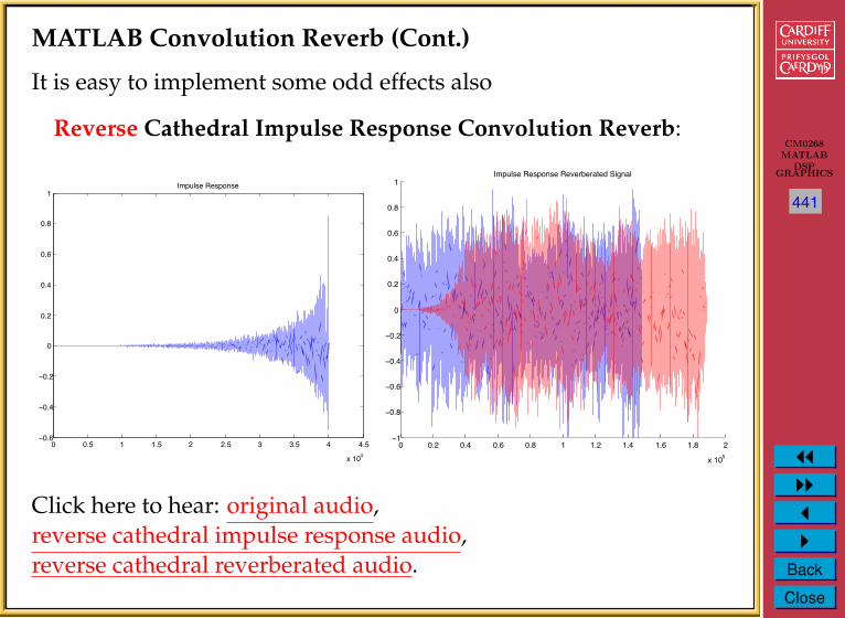
MATLAB Convolution Reverb (Cont.)

It is easy to implement some odd effects also

Reverse Cathedral Impulse Response Convolution Reverb:

0 0.5 1 1.5 2 2.5 3 3.5 4 4.5

x 104

−0.6

−0.4

−0.2

0

0.2

0.4

0.6

0.8

1Impulse Response

0 0.2 0.4 0.6 0.8 1 1.2 1.4 1.6 1.8 2

x 105

−1

−0.8

−0.6

−0.4

−0.2

0

0.2

0.4

0.6

0.8

1Impulse Response Reverberated Signal

Click here to hear: original audio,reverse cathedral impulse response audio,reverse cathedral reverberated audio.

CM0268MATLAB

DSPGRAPHICS

1

442

JJIIJI

Back

Close

MATLAB Convolution Reverb (Cont.)

You can basically convolve with anything:

Speech Impulse Response Convolution Reverb:

0 0.5 1 1.5 2 2.5 3 3.5 4 4.5

x 104

−0.8

−0.6

−0.4

−0.2

0

0.2

0.4

0.6

0.8Impulse Response

0 0.2 0.4 0.6 0.8 1 1.2 1.4 1.6 1.8 2

x 105

−1

−0.8

−0.6

−0.4

−0.2

0

0.2

0.4

0.6

0.8

1Impulse Response Reverberated Signal

Click here to hear: original audio,speech ‘impulse response’ audio, speech impulse reverberated audio.