HAL Id: hal-01242358https://hal.archives-ouvertes.fr/hal-01242358v1Preprint submitted on 15 Dec 2015 (v1), last revised 12 Jul 2017 (v4)

HAL is a multi-disciplinary open accessarchive for the deposit and dissemination of sci-entific research documents, whether they are pub-lished or not. The documents may come fromteaching and research institutions in France orabroad, or from public or private research centers.

L’archive ouverte pluridisciplinaire HAL, estdestinée au dépôt et à la diffusion de documentsscientifiques de niveau recherche, publiés ou non,émanant des établissements d’enseignement et derecherche français ou étrangers, des laboratoirespublics ou privés.

Diffusiophoresis at the macro-scaleC. Mauger, R. Volk, N. Machicoane, M. Bourgoin, C. Cottin-Bizonne, C.

Ybert, F. Raynal

To cite this version:C. Mauger, R. Volk, N. Machicoane, M. Bourgoin, C. Cottin-Bizonne, et al.. Diffusiophoresis at themacro-scale. 2015. �hal-01242358v1�

Diffusiophoresis at the macro-scale

C. Mauger,1 R. Volk,2 N. Machicoane,2 M. Bourgoin,3, 2 C. Cottin-Bizonne,4 C. Ybert,4 and F. Raynal1

1LMFA, CNRS and Universite de Lyon, Ecole Centrale Lyon,INSA de Lyon and Universite Lyon 1, 69134 Ecully CEDEX, France

2Laboratoire de Physique, ENS de Lyon, CNRS and Universite de Lyon, 69364 Lyon CEDEX 07, France3LEGI, CNRS, Universite Joseph Fourier, Grenoble INP, 38041 Grenoble CEDEX 9, France

4Institut Lumiere Matiere, CNRS and Universite de Lyon,Universite Lyon 1, F-69622 Villeurbanne CEDEX, France

Diffusiophoresis, a ubiquitous phenomenon which induces particle transport whenever solute gra-dients are present, was recently put forward in the context of microsystems and shown to stronglyimpact colloidal transport (from patterning to mixing) at such scales. In the present work, we showexperimentally that this nanoscale-rooted mechanism can actually induce changes in the macro-scale mixing of colloids by chaotic advection. Rather than the usual decay of standard deviation ofconcentration, which is a global parameter, we use different multi-scale tools available for chaoticflows or intermittent turbulent mixing, like concentration spectra, or second and fourth momentsof probability density functions of scalar gradients. Not only those tools can be used in open flows(when the mean concentration is not constant), but also they allow for a scale by scale analysis.Strikingly, diffusiophoresis is shown to affect all scales, although more particularly the smallest one,resulting in a change of scalar intermittency and in an unusual scale bridging spanning more than 7orders of magnitude. Quantifying the averaged impact of diffusiophoresis on the macro-scale mix-ing, we finally explain why the effects observed can be made consistent with the introduction of aneffective Peclet number.

I. INTRODUCTION

Diffusiophoresis is responsible for transport of large colloidal particles under the action of solutes [1, 2]. In the caseof electrolyte (salt) gradients, as will be considered in the following, it involves two mechanisms, both connected tothe presence of the nanometric electrical double layer on the surface of the colloid [1]: the first is purely mechanicaland can be explained as a consequence of the existence of gradients of excess of osmotic pressure inside the doublelayer, while the second is related to electrophoresis of the particles under the electric field induced by the differencein mobility of positive and negative ions of the salt. Interestingly, both contributions lead to an additional transportterm for the colloids of the same type, proportional to ∇ logS, where S(x, t) is the concentration in salt [1] at positionx and time t; the total contribution is called the diffusiophoretic velocity, denoted vdp (equation 3). The equationsof motion are thus given by

∂S∂t

+∇ · Sv = Ds ∇2S, (1)

∂C∂t

+∇ · C(v + vdp) = Dc ∇2C, (2)

vdp = Ddp ∇ logS, (3)

where C(x, t) is the concentration in colloids, v(x, t) is the advecting velocity field, and Dc and Ds are the diffusioncoefficients of colloids and salt respectively; Ddp is called the diffusiophoretic diffusivity. This set of equations is onlyvalid if v is negligibly modified by the velocity of the colloids (one way coupling), i.e. if the colloidal concentration isnot too large; this is the case here. From equation 2, it is clear that colloidal concentration is coupled to that of salt viathe diffusiophoretic drift velocity (equation 2), while the salt evolves freely during the process (equation 1). Althoughthe colloids are transported by the total velocity field v+vdp (equation 2), diffusiophoresis in laminar mixing can notbe seen as a consequence of a large scale effect through a large ratio of velocity amplitudes Vdp/V , since it remainslower than 1% during the whole experiment (see equation 12 and discussion in paragraph III C); rather, it is related tocompressible effects through the diffusiophoretic velocity which is not divergence-free, as recently shown numerically[3]. Thus it has similarities with preferential concentration of inertial particles in turbulent flows [4, 5].In a recent article, Deseigne et al.[6] have studied how diffusiophoresis affects chaotic mixing in a micro-mixer (the

so-called staggered herringbone mixer [7], 200µm wide and 115µm high). Using only a global characterization —thenormalized standard deviation of concentration, a classical tool in mixing studies— they evidenced a diffusiophoreticeffect that was interpreted in terms of effective diffusivity (or effective Peclet number). Although constituting a proofof concept, diffusiophoresis was there acting at microns scales which admittedly remains a natural (and small) scalefor phoretic transport. Therefore the question of the robustness of this effect on mixing remained largely opened. Inparticular, one may wonder whether diffusiophoretic effects may extend to chaotic mixing at the macro-scale: will it

2

Continuous laser =488 nm

H

x

y

z

Mirror

(a)

14

3 2

Protocol:

-

-

-

-

1 3

2 4

3 1

4 2

(b)

Figure 1: (a) Scheme of the experimental setup; the square Hele-Shaw cell (L = 50mm) lies horizontally in the xy plane. (b)Time-periodic mixing protocol: i

O → jO indicates that at this step the fluid is pushed at i

O and pumped at jO during a lapse

of time T/4, with T the period of the flow-field. The figure displays the instantaneous patterns of a typical concentration field(colloids without salt). A movie showing the type of concentration patterns observed during the whole mixing process is alsoprovided as supplemental material [16].

be able to spread over all length scales or will it remain ineffectively confined at nano-to-micro small scales? Thisamounts to investigate the possibility of scale-to-scale couplings: while chaotic advection alone affects all scales of ascalar field from the large scale of the macro-container down to the smallest scalar length scale where diffusion is themost effective [8–15], what happens when coupling with diffusiophoresis, whose mechanism applies at the nanoscale?In addition to the very existence of the effect, the quantification of its global impact on mixing also needs to befurther investigated. Indeed, as recently discussed theoretically [3], diffusiophoresis is actually related to compressibleeffects that contain a much richer phenomenology than effective diffusivity concepts: the consistence of such effectiveapproaches thus remains open.In order to answer those questions we study diffusiophoresis in such a chaotic mixer at the macro-scale, that is, with

dimensions of the experiment escaping the ones of microsystems by 2 to 3 orders of magnitudes (up to 5 cm globalscale). In addition, rather than the usual decay of standard deviation of concentration, which is a global parameter, weapply a set of refined characterizing analyses, using different multi-scale tools available from the turbulence community,like concentration spectra (section IIIA), or second and fourth moments of probability density functions (PDF) ofscalar gradients (section III B). These more elaborated tools allow us to perform a scale by scale analysis and thusstudy how all scales of scalar field can be affected by diffusiophoresis. Finally, after evidencing the propagation ofdiffusiophoretic effects up to the macro-scale, we discuss the introduction of an effective Peclet number approach toquantify it.

II. DESCRIPTION OF THE EXPERIMENT

A. Experimental set up

Mixing takes place in a horizontal square Hele-Shaw cell of side L = 50mm and height h = 4mm, supplied by 4inlets/outlets (figure 1). Each inlet/outlet is pressure-driven using a flow controller (Fluigent, MFCS). At t = 0, aquantity of 0.2 ml of a fluorescent solution (either dye or colloidal suspension) is introduced via inlet 1 inside theHele-Shaw cell initially filled with water (or salted water, see later) using a syringe pump. The four inlets/outlets arethen pressurized under 100mbar, and fluid motion is carried out by successive pressurization and depressurizationof the inlets/outlets: a movie showing the mixing process is provided as supplemental material [16]. Successivedeformations of the scalar field are characterized by Planar Laser-Induced Fluorescence (PLIF): a continuous laser(Coherent Genesis MX SLM-Series, λ = 488 ± 3 nm) coupled to a cylindrical lens forms a laser sheet with a typicalthickness of the order of the cell height, so that the whole volume of the cell is illuminated. The choice of using athick laser sheet rather than a thin one localized at the mid-height of the cell will be discussed at the end of sectionIIC.

3

The fluorescence signal is recorded with a 14-bit camera (Nikon D700, 4200 px × 2800 px) whose lens (zoom 105mm)is equipped with a band reject filter (notch 488 ± 12 nm) corresponding to the laser wavelength. ISO sensitivity isset to lowest value in order to avoid noise, aperture to highest (i.e. f/3.5), with a shutter speed of 12.5 ms. Imageresolution in both horizontal directions (x or y) is about 19µm.px−1, while the depth of field is of the order of 1mm.Calibration for different fluorescent species and different concentrations showed a linear behavior between the lightintensity and the concentration of the species throughout the range studied.

B. Flow-rate and mixing

Chaotic advection is enabled via the time-periodic protocol illustrated in Figure 1b, with four stages of same durationT/4 each. When considering chaos efficiency in such a Hele-Shaw cell, the important parameter is the dimensionlesspulse volume α

α =qT

L2 h, (4)

where q is the flow-rate; α represents the volume of fluid displaced during one period compared to the volume of thechamber [17, 18]. For this particular mixing protocol, a global chaos (no visible regular region) is obtained for α ≥ 1.2[17, 19]. Because large values of α would imply rather high flow-rates (hence large Reynolds numbers) or large periodsT (hence very long mixing time [20]), we chose to consider the smallest value of interest α = 1.2.

In a Hele-Shaw cell, the Reynolds number Reh is classically based on the height h of the cell, i.e., with a typicalvelocity q/(hL) and kinematic viscosity ν,

Reh =q

Lν. (5)

Note that the Reynolds number inside the pipes connected to the inlets/outlets,

Repipes =4q

π d ν, (6)

with d = 1mm the diameter of the pipes, is quite higher. Because in the present case Repipes = 64 Reh, we setReh = 1 in order to avoid a large Reynolds number in the pipe and hence non reproducible experiments. Thiscorresponds to a flow-rate q = 50µL s−1, and, providing α = 1.2, we obtain the smallest period T = 120 s; this isthe period we used. Note that with those parameters, the flow is totally laminar and deterministic, as can also beappreciated on the movie [16]. As a consequence, the advecting velocity v in equations 1 and 2 is identical for all thecases considered here (except for the short initial transient stratification, discussed in annexe A for cases with salt).Each of the experiments in this article was carried out twice, so as to avoid any error: because of its repeatability,the results obtained (Taylor scale, effective Peclet numbers, etc.) were identical for both runs.

Since we are interested in mixing, the relevant parameter is the Peclet number, that measures the relative effect ofadvection compared to diffusion; because in a Hele-Shaw flow with chaotic advection, mixing essentially takes placein the horizontal direction [21], we will consider thereafter the Peclet number based on the width L of the cell,

Pe =q

hD, (7)

with D the diffusion coefficient of the species considered.

C. Diffusiophoresis

For this study we used colloids of diameter 200 nm (FluoSpheres, LifeTechnologies F8811), marked with a yellow-green fluorophore (wavelength 505/515 nm); in order to induce diffusiophoresis, we also used a 20mM solution of salt(LiCl). LiCl was shown in microfluidic experiments to have a stronger diffusiophoretic effect compared to other salts[2]. These same microfluidic experiments revealed that diffusiophoretic drift of this class of particles in a gradient ofLiCl induces a motion of the colloids from low to high salt concentration regions. In the following, we discuss theinterplay between mixing and diffusiophoretic drift by considering three different cases:

� reference: the colloids are injected inside pure water;

4

Species Diffusion coefficient [m2. s−1] Peclet number

Colloids 2. 10−12 6. 106

Dextran 3.6 10−11 3. 105

Fluorescein 4. 10−10 3. 104

Salt (LiCl) 1.4 10−9 9. 103

Table I: Species used, diffusion coefficients and corresponding Peclet numbers

� salt-in: the salt is introduced together with the colloids inside pure water; in this configuration diffusiophoresisshowed hypo-diffusion (delayed mixing) in the staggered herringbone micro-mixer [6].

� salt-out : the colloids are injected inside salted water; in this configuration diffusiophoresis showed hyper-diffusion(enhanced mixing) in the staggered herringbone micro-mixer.

For a more systematic exploration of Peclet number effects on the mixing process, other species (molecular) havealso been considered, namely fluorescein isothiocyanate (FITC) and fluorescent dextran 70 000 MW (LifeTechnologiesD1823). For such molecular species diffusiophoresis is not expected to play a role. They will be used to characterize theefficiency of mixing as a function of the Peclet number (at fixed geometry and flow forcing) in order to quantify possibledeviations from the trend potentially induced by diffusiophoresis in the case of colloids. The diffusion coefficients andcorresponding Peclet numbers for all species used in the experiment are available in table I: the variation amplitudeof the Peclet number is more than two orders of magnitude.Note from equation 1 that, whereas the concentration in colloids is coupled to that of salt, the concentration in

salt S freely evolves during the experiment. Thus the salt is fully mixed for t ≥ L2 h/(2q) ln(Pes) [22, 23], withPes = q/(hDs) the Peclet number for salt, that is t ∼ 900 s with our parameters. After that time diffusiophoresis nomore affects colloids (although the global effect is still visible, i.e. mixing enhancement or reduction [3]). In whatfollows we will restrict to times where diffusiophoresis is fully effective.Note finally that, because of buoyancy effects, the salt tends to rapidly stratify inside the cell (see appendix A).

Hence, although they are almost isodense with water, the colloids tend to go from mid-height where they are injectedtowards the bottom of the cell because of a vertical diffusiophoresis, following this salt gradient (appendix A). This“settling” of colloids, only visible when salt is present and which goes against the effective buoyancy (more saltedwater in the bottom being denser than colloids, that are isodense in pure water), already reveals a first macroscopiceffect of diffusiophoresis. Because it became difficult to follow the colloids at long times using a very thin laser sheet(they would eventually disappear below the sheet), and because the flow is quasi 2D, we chose to illuminate the wholecell. This kind of height-averaging can result in a loss of signal at very large wavenumbers, especially in the salt-incase; however the coupling of the parabolic flow with diffusion also leads to some vertical homogenization of the scalarfield in a Hele-Shaw cell, although mixing is much more rapid in the horizontal direction because of chaotic advection[21]. Indeed, we will see that we are still able to quantify a clear effect in terms of effective Peclet number.

III. RESULTS

When measuring mixing efficiency, the quantity commonly used is the rate of decay of standard deviation of theconcentration Cstd(t) =< (C− < C >)2 >1/2, or the non-dimensional standard deviation σ(t) = Cstd(t)/Cstd(t = 0)[24], where < . > stands for the spatial average. Indeed, without diffusiophoresis, the rate of decay of Cstd(t) is relatedto the presence of high scalar gradients through the equation

dC2std

dt= −2D < (∇C)2 > . (8)

Note that diffusion operates at all scales, but is much more efficient at small scale where the gradients are moreintense. In the following, as commonly done by fluid mechanicists, the quantity 1

2(C− < C >)2 = 1

2C2

std(t) is referredto as scalar energy, by analogy with the kinetic energy.Above all, chaotic advection involves a large range of scalar scales from the macro-scale of the experiment down to

the smallest length scale involved, while diffusiophoresis involves a mechanism at the nano-scale. Thus such a global

parameter as σ is not enough to explore this typically multi-scale coupled problem. For instance, does diffusiophoresisstrongly dissipate scalar energy at a very small scale, or else interact with the flow so as to dissipate more smoothly atall length scales involved? In addition, let us note that even for global characterization, σ would not be an appropriateparameter here anyway since the flow is an open flow (marked particles go in and outside the chamber through theinlet/outlets during the periodic mixing protocol, i.e. <C>(t) 6= cst).

5

100

102

100

10−2

10−4

10−6

10−8

1010−1

Eθ(k)

k (mm−1)

100

102

10−6

10−4

10−2

100

10-1

10

k2E

θ(k)

k (mm−1)

(a) (b)

Figure 2: (a) Instantaneous spectra of scalar energy (time t = 160 s); (b) Instantaneous dissipation spectra, same time. Opensymbols stand for cases without salt. ◦: reference case (no salt); �: salt-in; �: salt-out; ▽: fluorescein. The scalar energyspectrum and dissipation spectrum for fluorescein have been divided by 10.

In order to investigate the multi-scale properties of the scalar field, we used different tools more commonly availablefrom fluid mechanics community, and adapted for such a multi-scale process:

� the scalar energy spectrum Eθ(k) is a usual means in chaotic advection studies [11, 25–28]; it quantifies thescalar energy contained at a given wavenumber k = 2π/ℓ, where ℓ can be seen as the physical scale at which thescalar energy is calculated, i.e. the typical width of a scalar structure; it is linked to the global scalar energythrough the relation 1

2C2

std =∫∞

0Eθ(k) dk.

� PDFs of scalar gradients (more widely encountered in turbulent mixing [29, 30], see also [11, 31]); while global

dissipation of scalar energy is linked to scalar gradients through equation 8, such a parameter does allow toinvestigate whether dissipation occurs mainly with gradients quite close to the mean gradient (as can be seenfor instance with a gaussian distribution), or else is related to very intense local gradients, in which case we referto spatial intermittency. In the present study, each image (corresponding to a given time t) allows to obtainO(6. 106) scalar gradient values in each direction, further used to compute one PDF.

A. Scalar energy spectra

Instantaneous scalar energy spectra Eθ(k) are calculated from individual concentration fields at a given time by

using the 2D-Fourier-transform θ(kx, ky, t) of the reduced scalar field θ(x, y, t) = (C(x, y, t)− <C(x, y, t)>)/Cstd(t);in order to reduce aliasing due to non-periodic boundary conditions, a window-Hanning method was used. The 1Disotropic spectrum was then obtained by averaging over each k = (k2x + k2y)

1/2.Figure 2(a) shows typical instantaneous scalar energy spectra for the three configurations, reference case (without

salt), salt-in and salt-out. Clearly, the small amount of salt visibly impacts the whole spectrum, although small scalarscales are more affected than large scales (as for diffusion effects). In the salt-in case (solid squares), the spectrumextends further towards large wavenumbers (small scales) than the reference spectrum. This kind of behavior wouldalso be observed if considering the concentration spectrum of a species that diffuses less than the colloid we used.Indeed, since diffusion is directly related to scalar dissipation through equation 8, a smaller diffusion coefficient D(therefore a larger Peclet number) implies that the final scalar dissipation occurs with larger scalar gradients, i.e. atan even smaller lengthscale: the spectrum would also be shifted towards larger wavenumbers. In the salt-out case, theeffect is reversed, with a shift towards smaller wavenumbers. As a comparison and in order to show the influence of amuch smaller Peclet number, we have also plotted in the figure the spectrum of fluorescein, although it was dividedby 10 for clarity.The effect is even clearer when looking at the term k2 Eθ(k), proportional to the scale by scale dissipation budget

(figure 2(b)): diffusiophoresis obviously affects all lengthscales ranging roughly from the centimeter (k ≥ 0.8mm−1)down to the smallest scales resolved. Quite remarkably, this demonstrates that diffusiophoresis can indeed influence

6

X (mm)

Y (

mm

)

0 10 20 30 40

0

10

20

30

40

−15

−10

−5

0

5

10

15

(a)

gx

timet(s)

−20 0 20

100

200

300

400

−15

−10

−5

0

gi

log(P

DF)

(b)

Figure 3: Reference case with colloids (no salt); (a): instantaneous reduced gradient x-component, gx = (Gx− < Gx >)/Gx|std,where Gx = ∂C/∂x (at time t = 293 s). (b): time evolution of log(PDF) of all reduced gradient components gi, where gi standsfor gx and gy (PDF(gi) = 1/2[PDF(gx) + PDF(gy)]). The dotted line at t = 150 s corresponds to the moment when PDFsbecome reasonably periodic in time, so that time-averaging is conceivable.

mixing processes way beyond its nanometric roots or its micrometric classical influence. Combined with chaoticmixing multi-scale process, it can spread over more than 7 orders of magnitude in length scales and affect the globalsystem.However one should note that the previous diagnosis relies on an instantaneous analysis: while the flow is time

periodic, the large scale patterns –and therefore the large scales of the associated spectra– also vary with time, as canbe appreciated on the movie included as supplemental material [16]. Indeed the effect is not always as pronounced asin figure 2, at some (rare) moments of the periodic cycle the effect is even reversed, as also found in our numericalsimulations [3]. Since most of the scalar energy is contained in larger scales (hence in small wavenumbers k), it istherefore not easy to obtain a time-averaged parameter from the concentration spectra that would accurately measurea global effect of salt. As observed in the spectra, small scalar scales are more affected by diffusiophoresis: we thereforepropose to investigate the concentration gradients, so as to obtain quantitative comparison that considers a globaleffect over time.

B. Concentration gradients

In order to obtain the concentration gradients G = ∇C, a given image of the concentration field (correspondingto a given time t) is first filtered using a Gaussian kernel to get rid of potential noise: filtering over two pixels(≈ 40µm) is fairly enough to obtain the gradients with great accuracy. Then we measure the two components of theconcentration gradients, Gx = ∂C/∂x and Gy = ∂C/∂y at each point of the image. For component x (respectivelyy), we calculate the mean gradient component over the whole image < Gx > (respectively < Gy >), and also the

standard deviation Gx|std =< (Gx− < Gx >)2 >1/2 (respectively Gy|std). In the following, we investigate the reducedgradient component gi:

gi = (Gi− < Gi >)/Gi|std , (9)

where i stands for x and y. In figure 3a we plot the reduced gradient x-component gx at a given time (t = 293 s,which corresponds to 2 1/4 periods of the flow-field) in the reference case (no salt). Note the very large amplituderange from −15 to 15, indicating that scalar gradient spatial fluctuations are not Gaussian (events of large amplitudeare more likely to happen than in a Gaussian case, which is usually referred to as spatial intermittency). This isreminiscent of the intense and intermittent gradient fronts produced by the mixing process, that are well capturedwhen computing this quantity. This results in stretched PDFs of scalar gradient as it will be shown later in figure4b. While gx and gy have equivalent statistics, it is interesting to consider the mean statistics that are even betterconverged: figure 3b shows the PDF of the normalized gradient component gi, PDF(gi) = 1/2[PDF(gx) + PDF(gy)],as a function of time (one PDF every second). In the experiment, after a transient mixing phase where the initialspot of marked dye begins to spread in the whole domain (roughly one period of the flow-field T ), the global patterns

7

104

105

106

107

100

λ(m

m)

Pe

(a)

−30 −20 −10 0 10 20 3010

−8

10−6

10−4

10−2

100

PDF(g

i)

gi

(b)

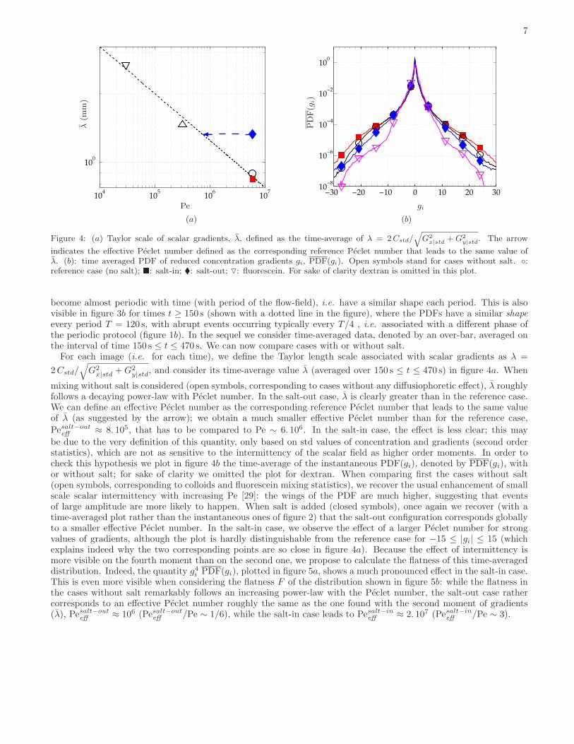
Figure 4: (a) Taylor scale of scalar gradients, λ, defined as the time-average of λ = 2Cstd/√

G2

x|std +G2

y|std. The arrow

indicates the effective Peclet number defined as the corresponding reference Peclet number that leads to the same value ofλ. (b): time averaged PDF of reduced concentration gradients gi, PDF(gi). Open symbols stand for cases without salt. ◦:reference case (no salt); �: salt-in; �: salt-out; ▽: fluorescein. For sake of clarity dextran is omitted in this plot.

become almost periodic with time (with period of the flow-field), i.e. have a similar shape each period. This is alsovisible in figure 3b for times t ≥ 150 s (shown with a dotted line in the figure), where the PDFs have a similar shapeevery period T = 120 s, with abrupt events occurring typically every T/4 , i.e. associated with a different phase ofthe periodic protocol (figure 1b). In the sequel we consider time-averaged data, denoted by an over-bar, averaged onthe interval of time 150 s ≤ t ≤ 470 s. We can now compare cases with or without salt.

For each image (i.e. for each time), we define the Taylor length scale associated with scalar gradients as λ =

2Cstd/√

G2x|std +G2

y|std, and consider its time-average value λ (averaged over 150 s ≤ t ≤ 470 s) in figure 4a. When

mixing without salt is considered (open symbols, corresponding to cases without any diffusiophoretic effect), λ roughlyfollows a decaying power-law with Peclet number. In the salt-out case, λ is clearly greater than in the reference case.We can define an effective Peclet number as the corresponding reference Peclet number that leads to the same valueof λ (as suggested by the arrow); we obtain a much smaller effective Peclet number than for the reference case,

Pesalt−outeff ≈ 8. 105, that has to be compared to Pe ∼ 6. 106. In the salt-in case, the effect is less clear; this may

be due to the very definition of this quantity, only based on std values of concentration and gradients (second orderstatistics), which are not as sensitive to the intermittency of the scalar field as higher order moments. In order tocheck this hypothesis we plot in figure 4b the time-average of the instantaneous PDF(gi), denoted by PDF(gi), withor without salt; for sake of clarity we omitted the plot for dextran. When comparing first the cases without salt(open symbols, corresponding to colloids and fluorescein mixing statistics), we recover the usual enhancement of smallscale scalar intermittency with increasing Pe [29]: the wings of the PDF are much higher, suggesting that eventsof large amplitude are more likely to happen. When salt is added (closed symbols), once again we recover (with atime-averaged plot rather than the instantaneous ones of figure 2) that the salt-out configuration corresponds globallyto a smaller effective Peclet number. In the salt-in case, we observe the effect of a larger Peclet number for strongvalues of gradients, although the plot is hardly distinguishable from the reference case for −15 ≤ |gi| ≤ 15 (whichexplains indeed why the two corresponding points are so close in figure 4a). Because the effect of intermittency ismore visible on the fourth moment than on the second one, we propose to calculate the flatness of this time-averageddistribution. Indeed, the quantity g4i PDF(gi), plotted in figure 5a, shows a much pronounced effect in the salt-in case.This is even more visible when considering the flatness F of the distribution shown in figure 5b: while the flatness inthe cases without salt remarkably follows an increasing power-law with the Peclet number, the salt-out case rathercorresponds to an effective Peclet number roughly the same as the one found with the second moment of gradients(λ), Pesalt−out

eff ≈ 106 (Pesalt−outeff /Pe ∼ 1/6), while the salt-in case leads to Pesalt−in

eff ≈ 2. 107 (Pesalt−ineff /Pe ∼ 3).

8

−30 −20 −10 0 10 20 300

1

2

3

4

g4 iPDF(g

i)

gi

(a)

104

105

106

107

101

Pe

Fla

tness

(b)

Figure 5: (a): g4i PDF(gi), where PDF(gi) is the time-averaged PDF of gi for the cases under study. (b): flatness of the timeaveraged PDF, F = (

∫

g4i PDF(gi) dgi)/(∫

g2i PDF(gi) dgi)2, with ‖gi‖ ≤ 30). The arrows indicate the effective Peclet numbers

defined as the corresponding reference Peclet numbers that lead to the same flatness. Open symbols stand for cases withoutsalt. ◦: reference case (no salt); �: salt-in; �: salt-out; △: dextran; ▽: fluorescein.

C. Discussion

Overall, our experimental results evidence that nano-scale diffusiophoresis is able to affect large particles mixing atthe macro-scale. More precisely, using a multi-scale approach to interpret our experimental results, we have shownthat diffusiophoresis affects all scales of the scalar field, although small scales are even more affected: because thesame could be said for diffusion, the effect of diffusiophoresis on the scalar field has some similarities with diffusiveeffects. This provides a clue as to why it is useful and meaningful to introduce an effective Peclet number whenconsidering the long time effects, and to try to quantify the combined effects of diffusiophoresis and diffusion withthat effective approach.We now compare quantitatively our results on the global influence of diffusiophoresis at the macro-scale with the

one obtained at the micro-scale with the herringbone micro-mixer by Deseigne et al. [6]. Although the flow-field inthe herringbone micro-mixer is stationary and 3-dimensional, it may however be compared favorably with what canbe expected in a two-dimensional time-periodic flow: indeed, Stroock & McGraw [32] proposed an analytical modelin which the cross-section of the channel is treated as a lid-driven cavity flow; they showed that this model was ableto reproduce the advection patterns that were observed experimentally in their flow, whose dimensions are about thesame as in Deseigne et al. (roughly 200µm wide, 100µm high). Here, because of the spatial periodicity in the axialdirection, the corresponding coordinate plays the role of time.When considering the experiment in the staggered herringbone micro-mixer, the effect is rather more important

than in the present case. In their case they obtained Pesalt−outeff /Pe ∼ 1/40 and Pesalt−in

eff /Pe ∼ 20. Note however

that in both experiments the effect is twice more important in the salt-out than in the salt-in case, i.e. Pe2 =2Pesalt−out

eff Pesalt−ineff .

There are different explanations for the shift between both experiments. Above all, remember that the present flowis an open flow (<C>(t) 6= cst), while the other one is not (<C > (t) = cst in all planes perpendicular to the axialdirection): colloids and salt go in and out of the cell, which could make the effect less important because of dilution.Indeed, in a perfect Stokes flow without diffusion, a fluid particle that enters into one of the pipes during one stageof the periodic flow-field would not move in the following stage, and finally come back to its original position in thechamber at the end of the next stage [19]. In the pipes, because of diffusion and small inertial effects, particles mayslightly move and sometimes remain in the pipes when the flow is reversed.

This may also come from the kind of “height-averaging” when illuminating the whole cell, that could make thehigher gradients slightly underestimated.Another reason could be related to the value of the Peclet number in the micro-mixer, that has to be based on

the cross-sectional velocity rather than on the axial velocity for a legitimate comparison. With their model, Stroock& McGraw could also estimate the magnitude of the velocity ucross in the cross-sectional flow relative to the axialvelocity U : taking ucross ∼ 0.1U , with a channel width w = 200µm and U = 8.6mm/s, we obtain a colloidal Peclet

9

number Pe ∼ 9. 104, that is, much smaller than in the present article (6. 106).In order to check if the difference in Peclet number could induce some of the shift observed, we propose to estimate

the order of magnitude of the diffusiophoretic term: from equation 3, we obtain

Vdp ∼ Ddp

ℓs, (10)

with ℓs the typical length-scale of salt gradients, resulting from a competition of contraction by the chaotic flow-fieldand diffusion. Because the salt is not coupled to the colloids, it verifies [22]:

ℓs ∼L√Pes

, (11)

where Pes is the salt Peclet number. Finally, from equations 10 and 11, we obtain:

Vdp

V∼ Ddp√

Dc Ds

Pe−1/2 ; (12)

this order of magnitude is in accordance with what we found numerically [3] (with the parameters used for ournumerical study we obtain from equation 12 that Vdp/V ∼ 4. 10−3 while we found numerically 7. 10−3). Note thatwith the colloids used for the experiment we have Ddp = 2.9 10−10 m2. s−1, so that we obtain from equation 12 aneven smaller ratio Vdp/V ∼ 2.2 10−3. Since the colloids are transported by the total velocity field v+vdp (equation 2),and since the relative effect of diffusiophoresis decreases with the Peclet number (equation 12), this could also explainpart of the shift (the relative effect is 8 times larger in the micro-mixer because of the difference in Peclet number).Note however that equation 12 can not be used to measure directly the difference in effective Peclet numbers: indeed,the effective Peclet number does not result from diffusiophoresis effects only, but also from diffusion effects, whoserelative strength compared to transport by the velocity field also decreases with the Peclet number from its verydefinition.Finally, let us note that although useful and convenient, this effective Peclet approach is only approximate, and is

best grounded for the salt-out configuration where mixing is enhanced. In that respect, it is quite remarkable thatthe effective Peclet for the salt-out case is indeed robust against the experimental observable used, either the Taylorscale of scalar gradients or the flatness of the distribution.As a matter of fact, strictly speaking diffusiophoresis is not a diffusive effect. Indeed we have clearly shown in

a recent numerical work [3] that a more general framework relates to the flow compressibility, and that a globalparameter like the standard deviation of concentration σ could increase at small times in the salt-in case, whereasdiffusion can only cause σ to decrease with time (equation 8). This is especially the case for the salt-in case wherediffusiophoresis acts against diffusion, effectively inducing an “anti-diffusion” that reinforces gradients at early times.This is the reason why salt-in characteristics do not show up as easily in averaged quantities, and require going to thefourth order moment of the distribution of gradients, rather than the Taylor scale associated to the second moment.

IV. SUMMARY

In this article we have studied experimentally the effects of diffusiophoresis on chaotic mixing of colloidal particlesin a Hele-shaw cell at the macro-scale. We have compared three configurations, one without salt (reference), onewith salt with the colloids (salt-in), and a third one where the salt is in the buffer (salt-out). Rather than the usualdecay of standard deviation of concentration, which is a global parameter, we have used different multi-scale toolslike concentration spectra, second and fourth moments of the PDFs of scalar gradients, that allow for a scale by scaleanalysis; those tools are also available in open flows, when marked particles can go in and out the domain under study.

Using scalar spectra, we have shown qualitatively that diffusiophoresis affects all scalar scales. This demonstratesthat this mechanism at the nano-scale has an effect at the centimetric scale, i.e. 7 orders of magnitude larger.Because the smallest scalar scales are more affected, this results in a change of spatial intermittency of the scalar:using second and fourth moments of the PDFs of scalar gradients, we have been able to quantify globally the impact ofdiffusiophoresis on mixing at the macro-scale. Although diffusiophoresis is clearly related to compressibility, we haveexplained how the combined effects of diffusiophoresis and diffusion are consistent when averaging in time with theintroduction of an effective Peclet number: the salt-in configuration corresponds to a larger effective Peclet numberthan the reference case, and the opposite for the salt-out configuration. Because this results from a time-averagedstudy, and not from an instantaneous diagnostic, this demonstrates that diffusiophoresis, whose mechanism appliesat the nanoscale, has a quantitative effect on mixing at the macro-scale.

10

Acknowledgments

This collaborative work was supported by the LABEX iMUST (ANR-10-LABX-0064) of Universite de Lyon, withinthe program “Investissements d’Avenir” (ANR-11-IDEX-0007) operated by the French National Research Agency(ANR).

Appendix A: Stratification of salt and associated migration of colloids

As seen in section IIC, salt induces a rapid stratification of the flow. This can be explained using characteristictime scales: the typical buoyancy time scale τA for a less dense particle at the bottom to reach the top of the cellis given by the Archimedes’ principle, ∆ρ g = ρh/τ2A, where g is gravity, ρ is density, and ∆ρ = ρβ∆C is linked tothe difference of salt concentration ∆C through the expansion coefficient β. With β = 2.4 10−2M−1 for LiCl [33] and∆C = 20mM, we obtain τA ≃ 0.92 s. While the viscous time scale τv that tends to dump the vertical velocity isτv = h2/ν = 16 s, and the diffusion time scale τd that tends to erase concentration gradients in the vertical directionby diffusion is τd = h2/Ds ∼ 3 h, the Rayleigh number of the flow, Ra = τv τd/τ

2A = β∆C g h3/(ν Ds) ∼ 216 000, is

way higher than the critical value. However, unlike Rayleigh-Benard convection, we have no source of buoyancy inthis experiment, so that the vertical movement stops (typically after time τv) when all heavy fluid has fallen at thebottom while the lighter fluid is at the top: the fluid is rapidly stratified inside the cell.

Once this stable stratification is set, a vertical gradient of salt appears, that can settle a colloid movement because ofdiffusiophoresis. Following equation 3, the vertical diffusiophoretic velocity, vdp ∼ Ddp ∇S/S ∼ Ddp/h. The typicaltime scale τvertdp associated to vertical diffusiophoresis is the time taken for a particle to go from half-depth where it

is injected down to the bottom, hence τvertdp ∼ h2/(2Ddp) ∼ 8 h. Although this is rather long, we could observe, when

using a very thin laser sheet (300µm-thick) that colloids tended to disappear below the sheet at large times. This iswhy we chose to illuminate the whole cell.

[1] J. L. Anderson. Colloid transport by interfacial forces. Annu. Rev. Fluid. Mech., 21, 1989.[2] B. Abecassis, C. Cottin-Bizonne, C. Ybert, A. Ajdari, and L. Bocquet. Osmotic manipulation of particles for microfluidic

applications. New Journal of Physics, 11(7):075022, 2009.[3] R. Volk, C. Mauger, M. Bourgoin, C. Cottin-Bizonne, C. Ybert, and F. Raynal. Chaotic mixing in effective compressible

flows. Phys. Rev. E, 90:013027, Jul 2014.[4] M. Maxey. The Gravitational Settling Of Aerosol-Particles In Homogeneous Turbulence And Random Flow-Fields. Journal

of Fluid Mechanics, 174:441–465, 1987.[5] R. A. Shaw. Particle-Turbulence interactions in atmospheric clouds. Annual Review of Fluid Mechanics, 35:183–227, 2003.[6] J. Deseigne, C. Cottin-Bizonne, A. D. Stroock, L. Bocquet, and C. Ybert. How a ”pinch of salt” can tune chaotic mixing

of colloidal suspensions. Soft Matter, 10:4795–4799, 2014.[7] A. D. Stroock, S. K. W. Dertinger, A. Ajdari, I. Mezic, H. A. Stone, and G. M. Whitesides. Chaotic Mixer for Microchannels.

Science, 295:647–651, 2002.[8] H. Aref. Stirring by chaotic advection. J. Fluid Mech., 143:1–21, 1984.[9] J.M. Ottino. The Kinematics of Mixing: Stretching, Chaos and Transport. Cambridge University Press, New-York, 1989.

[10] V. Rom-Kedar, A. Leonard, and S. Wiggins. An analytical study of the transport, mixing and chaos in an unsteadyvortical flow. J. Fluid Mech., 214:347–394, 1990.

[11] R. T. Pierrehumbert. Tracer microstructure in the large-eddy dominated regime. Chaos, Solitons & Fractals, 4(6):1091–1110, 1994.

[12] S. Cerbelli, A. Adrover, and M. Giona. Enhanced diffusion regimes in bounded chaotic flows. PHys. Let. A, 312:355–362,2003.

[13] E. Gouillart, J-L Thiffeault, and M. D. Finn. Topological mixing with ghost rods. Phys. Rev. E, 73:036311, Mar 2006.[14] D. R. Lester, G. Metcalfe, and M. G. Trefry. Is chaotic advection inherent to porous media flow? Phys. Rev. Lett.,

111:174101, Oct 2013.[15] O. Gorodetskyi, M.F.M. Speetjens, and P.D. Anderson. Eigenmode analysis of advective-diffusive transport by the compact

mapping method. European Journal of Mechanics - B/Fluids, 49, Part A:1 – 11, 2015.[16] See supplemental material at [CollRefFin-crop.avi] , movie showing the type of concentration patterns observed in the

time-periodic flow-field (T = 120 s), here in the reference case (colloids without salt).[17] F. Raynal, A. Beuf, F. Plaza, J. Scott, Ph. Carriere, M. Cabrera, J.-P. Cloarec, and E. Souteyrand. Towards better DNA

chip hybridization using chaotic advection. Phys. Fluids, 19:017112, 2007.[18] A. Beuf, J. N. Gence, Ph. Carriere, and F. Raynal. Chaotic mixing efficiency in different geometries of hele-shaw cells.

Int. J. Heat Mass Transfer, 53:684–693, 2010.

11

[19] F. Raynal, F. Plaza, A. Beuf, Ph. Carriere, E. Souteyrand, J.-R. Martin, J.-P. Cloarec, and M. Cabrera. Study of a chaoticmixing system for DNA chip hybridization chambers. Phys. Fluids, 16(9):L63–L66, 2004.

[20] F. Raynal and J.-N. Gence. Efficient stirring in planar, time-periodic laminar flows. Chem. Eng. Science, 50(4):631–640,1995.

[21] F. Raynal, A. Beuf, and Ph. Carriere. Numerical modeling of DNA-chip hybridization with chaotic advection. Biomi-crofluidics, 7(3):034107, 2013.

[22] F. Raynal and J.-N. Gence. Energy saving in chaotic laminar mixing. Int. J. Heat Mass Transfer, 40(14):3267–3273, 1997.[23] E. Villermaux, A. D. Stroock, and H. A. Stone. Bridging kinematics and concentration content in a chaotic micromixer.

Physical Review E, 77(1):015301, 2008.[24] E. L. Paul, V. A. Atiemo-obeng, and S. M. Kresta, editors. Handbook of Industrial Mixing: Science and Practice. Wiley

Interscience, 2003.[25] B. S. Williams, D. Marteau, and J. P. Gollub. Mixing of a passive scalar in magnetically forced two-dimensional turbulence.

Physics of Fluids (1994-present), 9(7):2061–2080, 1997.[26] V. Toussaint, Ph. Carriere, J. Scott, and J.-N. Gence. Spectral decay of a passive scalar in chaotic mixing. Phys Fluids,

12(11):2834–2844, 2000.[27] M.-C. Jullien, P. Castiglione, and P. Tabeling. Experimental observation of batchelor dispersion of passive tracers. Phys.

Rev. Lett., 85:3636–3639, Oct 2000.[28] P. Meunier and E. Villermaux. The diffusive strip method for scalar mixing in two dimensions. Journal of Fluid Mechanics,

662:134–172, 11 2010.[29] M. Holzer and E. D. Siggia. Turbulent mixing of a passive scalar. Physics of Fluids, 6(5):1820–1837, 1994.[30] Z. Warhaft. Passive scalars in turbulent flows. Annual Review of Fluid Mechanics, 32(1):203–240, 2000.[31] R. T. Pierrehumbert. Lattice models of advection-diffusion. Chaos, 10(1):61–74, 2000.[32] A. D. Stroock and G. J. McGraw. Investigation of the staggered herringbone mixer with a simple analytical model. Philo-

sophical Transactions of the Royal Society of London A: Mathematical, Physical and Engineering Sciences, 362(1818):971–986, 2004.

[33] CRC handbook of chemistry and physics, 92nd ed. CRC Press, Boca Raton, FL, 2011.