differential transforms and circuit theorykushnero/temp/pukhov.pdf · the application of these...

CIRCUIT THEORY AND APPLICATIONS, VOL. 10, 265-276 (1982)

DIFFERENTIAL TRANSFORMS AND CIRCUIT THEORY

GEORGII EVG. PUKHOV

The Institute of Simularion Problems in Energetics, Academy of Sciences of the Ukrainian SSR, Kiev, U.S.S.R.

SUMMARY

The function and equation transformations are presented where the transfer to images is made by means of differentiation. The application of these differential transforms for the design of linear and non-linear circuits is also discussed.

INTRODUCTION

Several problems of electrical engineering, automatization and electronics are successfully resolved using integral Laplace and Fourier transforms.' These transforms are mostly used in studying systems with constant parameters. In the integral transforms the images are defined by means of function integration. In the present work the images are found using function differentiation. Therefore they are referred to

-. as differential transform^."^ The mathematical formulae and rules of differential transforms allow the creation of both analytical and numerical methods for solving linear and non-linear systems.

DIRECT AND INVERSE DIFFERENTIAL TRANSFORMS

Consider the function x = x ( t ) of a real continuous variable t. It may be represented by an absolutely convergent Taylor series within the interval It, < It1 < Iti-tpl where t = ti is its centre and p is a convergence radius. The following relations may be written:

where M ( k ) # 0 is a scale function of integer argument k = 0 ,1 ,2 , . . . , a, and T = t - ti is the continuous argument from the point t = ti. The expression on the left side of correspondence symbol is a direct transform. It allows one to find the discrete image function Xi(k) of integer argument k by means of x ( t ) =x( t i +r) . The expression on the right side of the symbol is an inverse transform and it allows

.I one to use the discrete image values X;(O), X i ( l ) , . . . to find x ( t ) as a Taylor power series expanded about the point t = t i .

The discrete functions X,(k) are called T-functions and the differential transforms will be referred to briefly as T-transforms, since the functions are reconstructed in terms of discrete values of the image on the basis of Taylor's formula.

ELEMENTARY T-FUNCTIONS

Equation ( 1 ) shows that the form of the T-function depends on the scale function M ( k ) . Let

where H is a certain positive constant with the dimension of the argument, t, i.e. [HI = [ t ] .

- 0098-9886/82/030265-12$01.20 @ 1982 by John Wiley & Sons, Ltd.

Received 11 June 1980 Revised 1 March 1982

266 GEORGII EVG. PUKHOV

With such M ( k ) it may be seen that the images of a the product of functions (as of the most usable non-linear operation) are the simplest and moreover, all the discrete values of X;(k) have the same ' dimension, i.e. [Xi(0)] = [X,(l)] =. . . = [Xi(m)].

The transforms (1) take the form

with a scale function as given in (2). Substitution of the elementary functions such as 1, t = ti + T, tm, ec', sin o t and others simply defines

the corresponding images. 1. The image of the function which is everywhere unity (x(t) = 1) has the form

The discrete function %(k) is called T-unit or briefly 'teda'. 2. The image of the linear function (x(t) = t) is

where

3. The image of the mth power function (x(t) = tm) is

where m is a positive integer and

Let ti = 0, then r m H m % ( k -m). 4. The image of exponential function (x(t) = eC') is

where c is a constant. 5. The image of the sine (x(t) = sin o t ) is

sin wt I- k!

where w is a constant. 6. The image of the cosine (x(t) = cos wt) is

(oH)k cos (?+-I,) cos wt '- k !

The images of other functions that may be represented as absolutely convergent Taylor power series are found in a similar way.

DIFFERENTIAL TRANSFORMS AND CIRCUIT THEORY 267

THE CHARACTERISTICS O F DIFFERENTIAL TRANSFORMS .& Some properties of differential transforms may be found directly from (3 ) .

1. When the function x ( t ) is multiplied by a constant c the image should be multiplied by the same number, i.e.

cx ( t ) 1 cXi ( k ) (10)

2 . The algebraic sum of the functions x ( t ) = X i ( k ) and y ( t ) = Y , ( k ) is consistent with the same sum of their images

3. The product of the functions x ( t ) and y ( t ) is transformed into the algebraic convolution of their images l = k

x ( t ) y ( t ) l X i ( k ) * Y i ( k ) = C Xi( l )Yi(k - I ) I = O

(12)

where * is a convolution symbol. The expression X i ( k ) * Y i ( k ) is called the T-product of the discrete functions X i ( k ) and Y i ( k ) .

4. The quotient of the functions x ( t ) and y ( t ) is transformed into the T-function Z i ( k ) :

where H is the symbol of T-division defined by the given recurrence formula. 5. The logic-algebraic operation in the region of images

referred to as T-differentiation, is consistent with differentiation of x ( t ) by the variable t = ti + T. 6. The logic-algebraic operation in the region of images

is consistent with the operation of obtaining the indefinite integral of x ( t ) by dt. Here Ci is an integration constant defined by means of additional conditions, 9-' is the symbol of indefinite T-integration.

7 . The operators 9 and 9 - I are mutually inverse in the sense that

8, The value of the function x ( t ) at the point t = ti is equal to the original discrete value of the image at the same point, i.e.

ti) =xi (O) . (17)

9. The value of the function x ( t ) at the point t = ti +H is equal to the image discrete sum at the point t = ti, i.e.

10. The value of the function x ( t ) at the point t = ti -H is equal to the difference of even and odd discrete sums at the point t = ti, i.e.


1 1 . The formulae nxi =

are the generalizations of the two preceding formulae. Here Xi is a vector; its components being the discrete image values

and I7, I 7 - I are triangular matrices

assuming t i+, - ti = H for any i = 0 , 1 , 2 , . . . . e

12. Consider the operation of function superposition. Let y = y ( x ) and x = x( t ) ; the function x( t ) being represented by a Taylor series in powers of t and y ( x ) by a Taylor series in powers of x. Then

Let the image of the mth power of z ( t ) = Z ( k ) be denoted by Z?(k) and the image of y ( x ) by Y i ( k ) = y[Xi(k)] . As (24) is transformed into the region of images we obtain

since x(t i) = Xi(0). Equation (25) shows that in order to obtain the image of a complex function y ( x ) , x ( t ) should be

replaced by Xi(k) and all usual operations by T-operations. 13. The image of x( t ) shifted by a constant h is

where

is the mth T-derivative of the function Xi(k) . 14. Any T-function may be expanded in the following series over tedas

15. The formula

x (ct) = c k~ ( k ) (29) m

allows one to obtain the image of a function x(ct) in terms of the known image of x( t ) , where c is a constant.


GENERAL T-EQUATIONS O F ELECTRIC CIRCUITS &

The characteristics of electric circuits with lumped values are generally defined by the system of non-linear implicit differential equations

where x(t) is the vector of voltages, currents and of other circuit parameters, y is the operator to show what mathematical operations are to be made with x(t), its derivatives over t and with other functions of t, e.g. source voltages and currents, variable resistances, variable inductance etc.

Any functions of time in circuit differential equations are assumed to be represented as absolutely convergent Taylor series in powers of t, and current-voltage, flux-current, charge-voltage and other characteristics of non-linear elements may be described by similar Taylor series of current, voltage, charge, flux-linkage powers. In this case, to transfer (30) to the image region it is reasonable to change formally all functions for their images and the usual mathematical operations for corresponding T- operations (T-multiplication, T-division, T-differentiation etc.). After dividing the integration interval into n-parts and performing all the operations given above, the T-equations of the circuit are obtained

L where i = 0 , 1 , 2 , . . . , n. These equations combined with initial conditions

are used to estimate the transient response of the circuit. These same equations being used together with periodicity conditions x(to+ T) = x(to) taking the form

xi+n(k) =Xi(k) (33)

in the image region for the given case, solve the problem of periodic response calculation; here i may be taken as 0 and n corresponds to the period end.

If the centre of function expansion in power series is chosen not at the origin of co-ordinates, (ti # O), then coupling equations of Xo and Xi similar to (20) and (21) should be added to above equations.

METHOD O F LOCAL EQUATIONS

Power series are known to closely approximate analytical functions in the immediate neighbourhood of @ the expansion centre at It - ti] << p, where p is a convergence radius.

When the interval over which the differential equations are to be solved is large enough, the power series may converge rather slowly. Then the solution may be obtained as follows.

The integration section (0, t,) is divided into some intervals and for each point its own local T-equation is composed. Any of the local equations serve to approximate the solutions in the neighbourhood of its expansion centre. When the coupling equation is added to local equations, a system is obtained which approximates the unknown solution better than in the case of a single equation.

If the interval (0, t,) is divided into n equal parts and the scale constant is H = t,/n, then the total system of T-equations consists of local coupling 'forward' equations (20) and of 'backward' coupling equations (21). The system of T-equations thus obtained is solved further together with initial conditions or with periodicity conditions with respect to initial discrete values Xi(0) of local images Xi(k). These values represent simultaneously the values of xi at the same points because xi = Xi(0).

With discrete function values Xi(k) available it is easy to represent the solution as a system of local power series.

P The method of local T-equations may be extended to circuits with piecewise characteristics (current-

voltage and others) of non-linear elements. Let us show this. The function which is referred to as functional


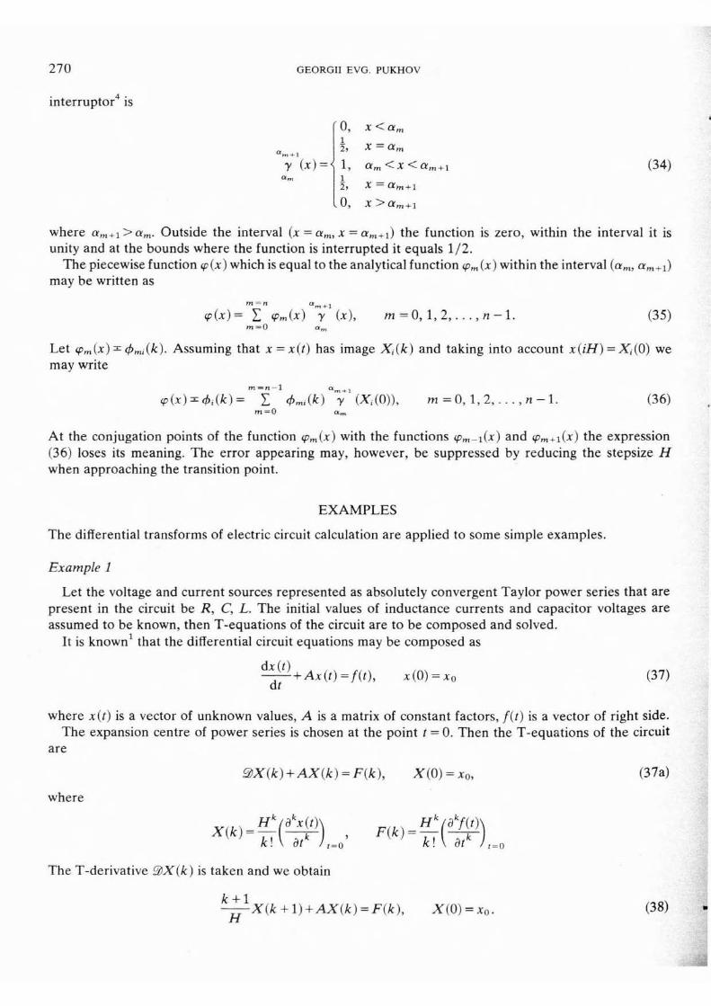
where >am. Outside the interval (x = a m , x = am+l) the function is zero, within the interval it is unity and at the bounds where the function is interrupted it equals 112.

The piecewise function cp(x) which is equal to the analytical function cpm (x) within the interval (a,, am+1) may be written as

m = n '=m+l

c p ( x ) = C cpm(x) y (x), m = O 7 l 7 2 , . . . , n - 1 .

Let cpm(x) #Jmi(k). Assuming that x = x(t) has image Xi(k) and taking into account x(iH) =Xi(0) we may write

At the conjugation points of the function cpm(x) with the functions ~ , - ~ ( x ) and V ~ + ~ ( X ) the expression (36) loses its meaning. The error appearing may, however, be suppressed by reducing the stepsize H when approaching the transition point.

EXAMPLES

The differential transforms of electric circuit calculation are applied to some simple examples.

Example 1

Let the voltage and current sources represented as absolutely convergent Taylor power series that are present in the circuit be R, C, L. The initial values of inductance currents and capacitor voltages are assumed to be known, then T-equations of the circuit are to be composed and solved.

It is known1 that the differential circuit equations may be composed as

where x(t) is a vector of unknown values, A is a matrix of constant factors, f(t) is a vector of right side. The expansion centre of power series is chosen at the point t = 0. Then the T-equations of the circuit

are

where

The T-derivative 9 X ( k ) is taken and we obtain

DIFFERENTIAL TRANSFORMS AND CIRCUIT THEORY 27 1

This expression allows us to calculate successively the discrete values of the function of X ( k ) . Indeed, assuming k = 0 , 1 , 2 , . . . we obtain

etc. The function x ( t ) relevant to these discrete values is obtained by means of the inverse transformation

This is a well known analytical solution of the above system of differential equations.

Example 2

Along with the constant parameters R, C, L, as voltage and current sources, the electrical circuit has also a time-varying resistor with r = r ( t ) , of which the image exists:

1

The T-equations of the circuit are to be composed and solved in the form of truncated power series. Consider the RLC circuit as a one-port network and r ( t ) as a load on this one-port network; then the

differential equations are composed.

where e ( t ) is the idle voltage of two-terminal network and Z ( p ) is a rational fraction of the form

where ai, bi are constants. Substituting p-operators by T-derivatives in (40) and using the notations

we can write

where \

l = k

R ( k ) * I ( k ) = 1 R ( l ) I ( k - 1 ) I = O

The T-equation (41) solves the problem of estimation of the transient and periodic responses in the above circuit with time-varying resistance r ( t ) .


Let, for example, e( t) = E = const, Z ( p ) = pL and

(wH)ksin*), \ A ~ < I . r ( t ) = R o ( l + A sin wt) = R ~ ( % ( ~ ) + A - k ! 2

Here (41) becomes

whence

With io known all the remaining discrete values I ( k ) are evidently successively defined. When a periodic solution is sought I (0) is obtained from

which represents the periodicity condition i (T) = i(0) if H = T. In both cases the solution has the form

Example 3

Let the synchronous generator be connected with buses of infinite power through a transmission line. The motion of the generator rotor is known to be described under some assumptions in terms of the non-linear differential equation

dt2 +a- d 2 ~ ( t ) b sin rp(r) = p , Q(o) = qo, ) = Q;, 0 s t B t,,

dr 1 = ~

where a , b, p are constants and (0, t,,) is the interval within which the solution is sought. By transfering into the image region with centres at the points

the system of T-equations is obtained

where the two first discrete values of the image &(k) 4 ( iH + T) at i = 0 are known and are given by

4o(O) = 40, 4 0 0 ) = H4 b. The image & 4;(k) is obtained from following considerations. Note that

9 & q 5 i ( k ) = ~ o q 4 ~ ( k ) * % $ ~ ( k ) , 9c~c$i(k)=-&4i(k)*94i(k).

It is easy to generate the following recurrence formulae

DIFFERENTIAL TRANSFORMS AND CIRCUIT THEORY

where on the basis of (17) characteristics u

a 4 i ( 0 ) = ~ i n 4 i ( 0 ) , C O S ~ ~ ~ ( O ) = C ~ ~ ~ ~ ( O ) , i = O , l , 2 , . . . , n-1.

Now assume in the above formulae i = 0 and k = 0 , 1 , 2 , 3 , . . . , and the discrete values are successively obtained

In terms of the discrete values &(k) the power series may be found

which represent the solution in the neighbourhood of the point to = 0. L In order to obtain the power series as a solution in the neighbourhood of the point tl = H we do as follows.

Using 'forward' coupling equations

the discrete values 1$~(0) and d l ( l ) are obtained. All remaining discrete values d l ( k ) are found in exactly the same way, as it was with 40(k) in terms of two initial discrete values do(0) and do( l ) .

With the help of the discrete functional values d l (k ) the power series is obtained

which represents the solution in the neighborhood of the point tl = H. Coupling 'backward' equations

do(0) =4i(O)-41(1)+4i(2)-41(3)+. . . 40(1) =41(1)-241(2)+341(3)-.

40(2) = 41(2) - 341(3) +. . . make it possible to see how advantageously the number of discrete function values q50(k) and the step size H were chosen.

The transfer to power series for solutions in the neighbourhood of the points t2 = 2H, t3 = 3H, . . . , t, = nH is analogous.

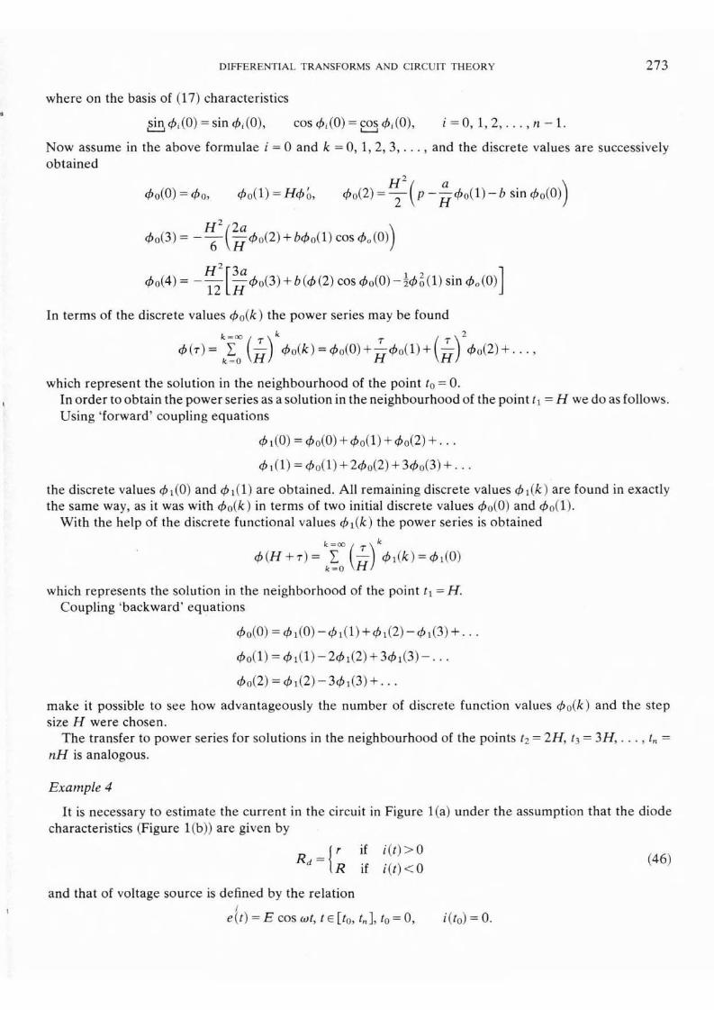
Example 4

It is necessary to estimate the current in the circuit in Figure l (a) under the assumption that the diode characteristics (Figure l(b)) are given by

and that of voltage source is defined by the relation I 1

e (t) = E cos wt, t E [to, t,,], to = 0, i(to) = 0.

GEORGII EVG. PUKHOV

Figure 1.

Using the methods for function interruptors (34), the differential equations of the circuit with piecewise- linear characteristics of the non-linear element (46) can be written in the form of a single formula

While transferring into the T-area we can obtain for the interval of independent variable t E [sH, ( s + 1 ) H ]

where s = 0, 1,2. . . , n - 1 and Io(0) = 0. In terms of above discrete values I , (k) the current values i ( t ) can be estimated at the moment t = ( s + l ) H

using the coupling 'forward' equation (20)

The calculations in terms of coupling 'backward' equations (21)

are checked only at Is(0) > 0 or at Is(0) < 0 since at I,(O) = 0 the diode current-voltage characteristics cannot be represented by Taylor series.

The set of local power series

defines the circuit current at any instant t = sH + r, 7 E [0, HI within the interval (0, t,).

Example 5

Let a periodic saw-tooth voltage be applied to a complex linear two-terminal network with R, L, C elements. The voltage is varied linearly e ( t ) =Et/T with period T (Figure 2). The steady state input current i ( t ) is to be defined.

( 0 ) ( b )

Figure 2.


In a circuit with constant parameters the operator p = dldt is substituted by the T-derivative and I currents and voltages are substituted by their images to obtain T-equations from differential equations.

When the transition function of the two-terminal network is Z ( p ) , the T-equation of the circuit has the form

z ( g ) I S ( k ) = Es(k) ,

where Z ( 9 ) is a rational fraction of the type

Let H = T and an expansion centre be at the beginning of a period (t, = 0 ) . Then

When (at H = T)

is taken into account, the T-equation becomes

To solve this equation it is reasonable to use the method of normal fundamental functions. " Because of the linearity of (48) it is evident that

I ( k ) = J ( k ) +&(k)I(O) + + ~ ( k ) I ( l ) + . . . + 4 , - l ( k ) I ( n - 1)

The functions J ( k ) and 4 , ( k ) are found directly from (48) , so

J ( k ) = I ( k ) if I ( 0 ) = I ( 1 ) = . . . = I (n - 1 ) = 0 ;

&(k) = I ( k ) if I ( 0 ) = 1, I ( 1 ) = I ( 2 ) = . . . = I ( n - 1 ) = 0 ; bo = bl = 0 ;

4 1 ( k ) = I ( k ) if I ( 0 ) = 0 , I ( 1 ) = 1, I ( 2 ) = . . . = I ( n - 1) = 0 ; bo = b1 = 0 .

When J ( k ) and 4 , ( k ) are defined and the periodicity conditions

are used for calculations, the discrete values I(O), I ( l ) , . . . , I ( n - 1 ) are found to provide the periodic response. Note that the above periodicity conditions hold only for two terminal networks where input current i ( t ) and its first (n - 1) derivatives over t are continuous and

dmi ( t ) dmi( t )

where m = 0 , 1, 2 , . . . , n - 1.

CONCLUSION

Even the small set of rules and formulae from the theory of differential transforms that were presented above shows that together with the well known integral transforms the differential transforms widen the


facilities for solving complex physical systems with the help of methods of mathematical simulation using computers.

The author advises use of the differential transforms for analysis and synthesis of electrical circuits and various electronic and automatic sets.

REFERENCES

1. Stephen W. Director and Ronald A. Roher, Introduction to System Theory, McGraw-Hill. 2 . r . E. ~ ~ X O B . npeo6pa3oea~ua Teiinopa u ax npuMeHeuue B sneKTpoTexHuKe u sneKrpouuKe. M3n. 'Hay~osa n y ~ r a ' , Knea,

1978. G. Evg. Puhkov, Taylor Transforms and their Application in Electrotechnics and Electronics, Naukova Dumka, Kiev, 1978.

3. r. E. nyxoe. Au@+epe~ouanb~b~e npeo6pa3oea~un (PYHKUUR u y p a ~ ~ e u u f i . Msn. 'Hay~osa nyura'. Kuea, 1980. G. Evg. Pukhov, Differential Transformations of Functions and Equations, Naukova Dumka, Kiev, 1980.

4. H. M . r e p c e ~ a ~ o e . Co6pa~ue C O ~ U H ~ H U ~ ~ , TOM 11. C T ~ O ~ ~ B O ~ H M O ~ U ~ ~ ~ T . Mocrsa, 1948. N. M. Gersevanov, Transactions, Vol. 11, Stroyvoenmorizdat, Moscow, 1948.

differential transforms and circuit theorykushnero/temp/pukhov.pdf · the application of these...

Documents