dielectric relaxation phenomena in complex systems...
TRANSCRIPT

THE KAZAN FEDERAL UNIVERSITY
INSTITUTE OF PHYSICS
DIELECTRIC RELAXATION PHENOMENA
IN COMPLEX SYSTEMS
Tutorial
Yu. Feldman, Yu.A. Gusev, M.A.Vasilyeva
Kazan 2012
Печатается по решению Редакционно-издательского совета ФГАОУВПО
«Казанский (Приволжский) федеральный университет»
методической комиссии Института физики
Протокол № от « » 2012 г.
заседания кафедры радиоэлектроники
Протокол № от « » 2012 г.
Авторы-составители
Yu. Feldman, Yu.A. Gusev, M.A.Vasilyeva
Научный редактор
д.ф.-м.н., проф. М.Н. Овчинников
Рецензент
д.х.н., проф. Ю.Ф. Зуев
Рецензент
к.ф.-м.н., доц. И.А. Насыров
Title: Dielectric Relaxation Phenomena in Complex Systems: Tutorial / Yu. Feldman,
Yu.A. Gusev, M.A.Vasilyeva. – Kazan: Kazan University, 2012. – p. 134.
In the writing of this tutorial we have not sought to cover every aspect of the dielectric
relaxation of complex materials. The aim of this work to demonstrate the usefulness of
dielectric spectroscopy for such systems, using its application on select examples as
illustrations. This tutorial will be helpful to students, graduate students and others who are
interested in the dielectric spectroscopy of complex systems.
© Kazan University, 2012
2
Contents 1. Introduction ................................................................................................................................................... 5 2. Dielectric Polarization, Basic Principles...................................................................................................... 7
2.1. Dielectric Polarization in Static Electric Fields........................................................................ 7 2.1.1. Types of Polarization ................................................................................................................................8
2.2. Dielectric Polarization in Time - Dependent Electric Fields .................................................. 11 2.2.1. Dielectric response in Frequency and Time Domains.............................................................................12
2.3. Relaxation kinetics ................................................................................................................. 16 3. Basic Principles of Dielectric Spectroscopy and Data Analyses .............................................................. 19
3.1. The Basic Principles of the BDS Methods ............................................................................. 20 3.2. The Basic Principles of the TDS Methods.............................................................................. 23
3.2.1. Experimental Tools.................................................................................................................................26 3.2.2. Data Processing ......................................................................................................................................30
3.3. Data analysis and fitting problems ......................................................................................... 30 3.3.1. The continuous parameter estimation problem .......................................................................................30 3.3.2. dc-Сonductivity problems.......................................................................................................................32 3.3.3. Continuous Parameter Estimation Routine .............................................................................................33 3.3.4. Computation of the dc-conductivity using Hilbert transform .................................................................33 3.3.5. Computing software for data analysis and modeling ..............................................................................35
4. Dielectric response in some disordered materials..................................................................................... 36 4.1. Microemulsions ...................................................................................................................... 37 4.2. Porous materials ..................................................................................................................... 42
4.2.1. Porous glasses.........................................................................................................................................42 4.2.2. Porous Silicon.........................................................................................................................................45
4.3. Ferroelectric crystals .............................................................................................................. 47 4.4. H-Bonding Liquids................................................................................................................. 51
5. Cooperative dynamic and scaling phenomena in disordered systems .................................................... 57 5.1.1. Porous glasses.........................................................................................................................................60 5.1.2. Porous silicon..........................................................................................................................................66
5.2. Dynamic percolation in ionic microemulsions ....................................................................... 68 5.2.1. Dipole correlation function for the percolation process ..........................................................................68 5.2.2. Dynamic hyperscaling relationship.........................................................................................................70 5.2.3. Relationship between the static and dynamic fractal dimensions ...........................................................74
5.3. Percolation as part of "Strange Kinetic" Phenomena ............................................................. 76 5.4. Universal scaling behavior in H-bonding networks ............................................................... 85
5.4.1. Glycerol-rich mixtures............................................................................................................................85 5.4.2. Water-rich mixtures ................................................................................................................................89
5.5. Liquid-like behavior in doped ferroelectric crystals............................................................... 97 5.6. Relaxation Kinetics of Confined Systems ............................................................................ 100
5.6.1. Model of relaxation kinetics for confined systems ...............................................................................100 5.6.2. Dielectric relaxation of confined water.................................................................................................102 5.6.3. Dielectric relaxation in doped ferroelectric crystal ...............................................................................104 5.6.4. Possible modifications of the model .....................................................................................................106 5.6.5. Relationships between the static properties and dynamics....................................................................108
3
5.7. Dielectric Spectrum Broadening in disordered materials ..................................................... 109 5.7.1. Symmetric Relaxation peak broadening in complex systems ...............................................................110 5.7.2. Polymer-water mixtures........................................................................................................................115 5.7.3. Micro-composite material .....................................................................................................................118
6. Summary .................................................................................................................................................... 122 7. Acknowledgements .................................................................................................................................... 122 8. References .................................................................................................................................................. 123
4
1 Introduction Recent years have witnessed extensive research of soft condensed matter physics to
investigate the structure, dynamics, and macroscopic behavior of complex systems (CS). CS
are a very broad and general class of materials that are typically non-crystalline. Polymers,
biopolymers, colloid systems (emulsions and microemulsions), biological cells, porous
materials, and liquid crystals can all be considered as CS. All of these systems exhibit a
common feature: the new "mesoscopic" length scale, intermediate between molecular and
macroscopic. The dynamic processes occurring in CS include different length and time scales.
Both fast and ultra-slow molecular rearrangements take place within the microscopic,
mesoscopic and macroscopic organization of the systems. A common theme in CS is that
while the materials are disordered at the molecular scale and homogeneous at the macroscopic
scale, they usually possess a certain amount of order at an intermediate, so-called mesoscopic,
scale due to a delicate balance of interaction and thermal effects. Simple exponential
relaxation law and the classical model of Brownian diffusion cannot adequately describe the
relaxation phenomena and kinetics in such materials. This kind of non-exponential relaxation
behavior and anomalous diffusion phenomena is today called “strange kinetics” [1,2].
Generally, the complete characterization of these relaxation behaviors requires the use of a
variety of techniques in order to span the relevant ranges in frequency. In this approach,
Dielectric Spectroscopy (DS) has its own advantages. The modern DS technique may overlap
extremely wide frequency (10-6 to 1012 Hz), temperature (- 170 °C to +500 °C) and pressure
ranges [3-5]. DS is especially sensitive to intermolecular interactions and is able to monitor
cooperative processes at the molecular level. Therefore, this method is more appropriate than
any other to monitor such different scales of molecular motions. It provides a link between the
investigation of the properties of the individual constituents of the complex material via
molecular spectroscopy and the characterization of its bulk properties.
This tutorial concentrates on the results of DS study of the structure, dynamics, and
macroscopic behavior of complex materials. First, we present an introduction to the basic
concepts of dielectric polarization in static and time dependent fields, before the Dielectric
Spectroscopy technique itself is reviewed both for frequency and time domains. This part has
three sections, i.e. Broad Band Dielectric Spectroscopy, Time Domain Dielectric
Spectroscopy and a section where different aspects of data treatment and fitting routines are
discussed in detail. Then, some examples of dielectric responses observed in various
disordered materials are presented. Finally, we will consider the experimental evidence of
5
non-Debye dielectric responses in several complex disordered systems such as
microemulsions, porous glasses, porous silicon, H-bonding liquids, aqueous solutions of
polymers and composite materials.
6

2 Dielectric Polarization, Basic Principles
2.1 Dielectric Polarization in Static Electric Fields
When placed in an external electric field E, a dielectric sample acquires a non-zero
macroscopic dipole moment. This means that the dielectric is polarized under the influence of
the field. The polarization P of the sample, or dipole density, can be presented in a very
simple way
VM
P = , (2.1)
where <M> is the macroscopic dipole moment of the whole sample volume V, which is
formed by the permanent micro dipoles (i.e. coupled pairs of opposite charges) as well as by
dipoles that are not coupled pairs of micro charges within the electro neutral dielectric sample.
The brackets < > denote ensemble average. In a linear approximation the macroscopic
polarization of the dielectric sample is proportional to the strength of the applied external
electric field E [6]:
kiki EP χε0= , (2.2)
where χik is the tensor of the dielectric susceptibility of the material and ε0 =8.854⋅10-12
[F⋅m-1] is the dielectric permittivity of the vacuum. If the dielectric is isotropic and uniform,
χ is a scalar and equation (2.2) will be reduced to the more simple form:
EP χε0= . (2.3)
According to the macroscopic Maxwell approach, matter is treated as a continuum, and
the field within the matter in this case is the direct result of electrical displacement (electrical
induction) vector D, which is the electric field corrected by polarization [7]:
D=ε0E+P. (2.4)
For an uniform isotropic dielectric medium, the vectors D, E, P have the same direction,
and the susceptibility is coordinate-independent, therefore
7

EED εεχε 00 )1( =+= , (2.5)
where χε += 1 is the relative dielectric permittivity. Traditionally, it is also called the
dielectric constant, because in a linear regime it is independent of the field strength. However,
it can be a function of many other variables. For example in the case of time variable fields it
is dependent on the frequency of the applied electric field, sample temperature, sample
density (or pressure applied to the sample), sample chemical composition, etc.
2.1.1 Types of Polarization
For uniform isotropic systems and static electric fields, from (2.3)-(2.5) we have
( )EP 10 −= εε . (2.6)
The applied electric field gives rise to a dipole density through the following
mechanisms:
Deformation polarization: It can be divided in the two independent types:
Electron polarization - the displacement of nuclei and electrons in the atom under the
influence of an external electric field. As electrons are very light they have a rapid
response to the field changes; they may even follow the field at optical frequencies.
Atomic polarization - the displacement of atoms or atom groups in the molecule under the
influence of an external electric field.
Orientation polarization: The electric field tends to direct the permanent dipoles. The
rotation is counteracted by the thermal motion of the molecules. Therefore, the orientation
polarization is strongly dependent on the frequency of the applied electric field and on the
temperature.
Ionic Polarization: In an ionic lattice, the positive ions are displaced in the direction of an
applied field while the negative ions are displaced in the opposite direction, giving a resultant
dipole moment to the whole body. The ionic polarization demonstrates only weak temperature
dependence and determines mostly by the nature of the interface where the ions can
accumulate. Many cooperative processes in heterogeneous systems are connected with ionic
polarization.
To investigate the dependence of the polarization on molecular quantities it is
convenient to assume the polarization P to be divided into two parts: the induced polarization
8
Pα, caused by translation effects, and the dipole polarization Pμ, caused by the orientation of
the permanent dipoles. Note that in the case of ionic polarization the transport of charge
carriers and their trapping can also create induced polarization.
( )EPP 10 −=+ εεμα . (2.7)
We can now define two major groups of dielectrics: polar and non-polar. A polar
dielectric is one in which the individual molecules possess a permanent dipole moment even
in the absence of any applied field, i.e. the center of positive charge is displaced from the
center of negative charge. A non-polar dielectric is one where the molecules possess no
dipole moment unless they are subjected to an electric field. The mixture of these two types of
dielectrics is common in the case of complex liquids and the most interesting dielectric
processes occur at their phase borders or liquid-liquid interfaces.
Due to the long range of the dipolar forces an accurate calculation of the interaction of a
particular dipole with all other dipoles of a specimen would be very complicated. However, a
good approximation can be made by considering that the dipoles beyond a certain distance,
say some radius a, can be replaced by a continuous medium having the macroscopic dielectric
properties. Thus, the dipole, whose interaction with the rest of the specimen is being
calculated, may be considered as surrounded by a sphere of radius a containing a discrete
number of dipoles. To make this approximation the dielectric properties of the whole region
within the sphere should be equal to those of a macroscopic specimen, i.e. it should contain a
sufficient number of molecules to make fluctuations very small [7,8]. This approach can be
successfully used also for the calculation of dielectric properties of ionic self-assembled
liquids. In this case the system can be considered as a monodispersed consisting of spherical
polar water droplets dispersed in a non-polar medium [9].
Inside the sphere where the interactions take place, the use of statistical mechanics is
required. To represent a dielectric with dielectric constant ε, consisting of polarizable
molecules with a permanent dipole moment, Fröhlich [6] introduced a continuum with
dielectric constant ε∞ in which point dipoles with a moment μd are embedded. In this model
μd has the same non-electrostatic interactions with the other point dipoles as the molecule
had, while the polarizability of the molecules can be imagined to be smeared out to form a
continuum with dielectric constant ε∞ [7].
In this case, the induced polarization is equal to the polarization of the continuum with
the ε∞, so that one can write:
9
( )EP 10 −= ∞εεα . (2.8)
The orientation polarization is given by the dipole density due to the dipoles μd. If we
consider a sphere with volume V containing dipoles, one can write:
><= dVMP 1
μ (2.9)
where is the average component in the direction of the field of the moment
due to the dipoles in the sphere.
( )∑=
= N
1iidd μM
In order to describe the correlations between the orientations (and also between the
positions) of the i-th molecule and its neighbors, Kirkwood [7] introduced a correlation factor
g, which was accounted as , where θij denotes the angle between the
orientation of the i-th and the j-th dipole. An approximate expression for the Kirkwood
correlation factor can be derived by taking only nearest-neighbor interactions into account. It
reads as follows:
∑=
><=N
jijg
1cosθ
><+= ijzg θcos1 . (2.10)
In this case the sphere is shrunk to contain only the i-th molecule and its z nearest neighbors.
Correlation factor g will be different from 1 when 0cos >≠< ijθ , i.e. when there is a
correlation between the orientations of neighboring molecules. When the molecules tend to
direct themselves with parallel dipole moments, >< ijθcos will be positive and g > 1. When
the molecules prefer to arrange themselves with anti-parallel dipoles, then g < 1. Both cases
are observed experimentally [6-8]. If there is no specific correlation then g = 1. If the
correlations are not negligible, detailed information about the molecular interactions is
required for the calculations of g.
For experimental estimation of the correlation factor g the Kirkwood-Fröhlich
equation [7]
( )( )( )2
02
229+
+−=
∞
∞∞
εεεεεεεμ
NTVkg B
d (2.11)
is used, which gives the relation between the dielectric constant ε , the dielectric constant of
induced polarization ∞ε . Here kB = 1.381⋅10-23 [J⋅K-1] is the Boltzmann constant, T is absolute
10
temperature. The correlation factor is extremely useful in understanding the short-range
molecular mobility and interactions in self assembled systems [10].
2.2 Dielectric Polarization in Time - Dependent Electric Fields
When an external field is applied to a dielectric, polarization of the material reaches its
equilibrium value, not instantaneously, but rather over a period of time. By analogy, when the
field is suddenly removed, the polarization decay caused by thermal motion follows the same
law as the relaxation or decay function of dielectric polarization φ(t):
)0()()(
PP tt =φ
, (2.12)
where P(t) is a time dependent polarization vector. The relationship for the dielectric
displacement vector D(t) in the case of time dependent fields may be written as follows
[6,11]:
( ) ( ) ( ) ⎥⎦
⎤⎢⎣
⎡′′−′Φ+= ∫
∞−
•
∞
t
tdttttt EED )(0 εε.
(2.13)
In (2.13) ( ) ( ) ( )ttt PED += 0ε , and Φ(t) is the dielectric response function
[ ])(1) t()(t s φεε −∞−=Φ , where εs and ε∞ are the low and high frequency limits of the
dielectric permittivity respectively. The complex dielectric permittivity ε*(ω) (where ω is the
angular frequency) is connected with the relaxation function by a very simple relationship
[6,11]:
⎥⎦⎤
⎢⎣⎡−=
−−
∞
∞ )(ˆ)(*t
dtdL
sφ
εεεωε
, (2.14)
where L is the operator of the Laplace transform, which is defined for the arbitrary time-
dependent function f(t) as:
.
(2.15) [ ]
unitimaginary an is and 0 where,
,)()()(ˆ0
ixixp
dttfeFtfL pt
→+=
=≡ ∫∞
−
ω
ω
11
Relation (2.14) shows that the equivalent information on dielectric relaxation
properties of the sample being tested both in frequency and time domain. Therefore the
dielectric response might be measured experimentally as a function of frequency or time,
providing data in the form of a dielectric spectrum ( )ωε * or the macroscopic relaxation
function ( )tφ . For example, when macroscopic relaxation function obeys the simple
exponential law
)/exp()( mtt τφ −= , (2.16)
where τm represents the characteristic relaxation time, the well-known Debye formula for the
frequency dependent dielectric permittivity can be obtained by substitution (2.16) into (2.15)
[6-8,11]:
ms iωτεεεωε
+=
−−
∞
∞1
1)(*
. (2.17)
For many of the systems being studied, the relationship above does not sufficiently describe
the experimental results. The Debye conjecture is simple and elegant. It enables us to
understand the nature of dielectric dispersion. However, for most of the systems being
studied, the relationship above does not sufficiently describe the experimental results. The
experimental data is better described by non-exponential relaxation laws. This necessitates
empirical relationships, which formally take into account the distribution of relaxation times.
2.2.1 Dielectric response in Frequency and Time Domains
In the most general sense non-Debye dielectric behavior can be described in terms of a
continuous distribution of relaxation times, G(τ) [11]. This implies that the complex dielectric
permittivity can be presented as follows:
( ) ( )∫∞
∞
∞
+=
−−
0
*
1τ
ωττ
εεεωε d
iG
S , (2.18)
where the distribution function G(τ) satisfies the normalization condition
12

( ) 10
=∫∞
ττ dG .
(2.19)
The corresponding expression for the decay function is
( ) ( ) ττ
τφ dtGt ⎟⎠⎞
⎜⎝⎛ −= ∫
∞
exp0 .
(2.20)
It must be clearly understood that by virtue of the univalent relationship (2.14) between
frequency and time representation the G(τ) calculation does not provide in itself anything
more than another way of describing the dynamic behavior of dielectrics in time domain [12].
Moreover, such a calculation is a mathematically ill-posed problem [13,14], which leads to
additional mathematical difficulties.
In most cases of non-Debye dielectric spectrum has been described by the so-called
Havriliak-Negami (HN) relationship [8,11,15]:
[ ]βαωτ
εεεωε
)(1)(*
m
s
i+
−+= ∞
∞ , 0 ≤ α, β ≤ 1 . (2.21)
Here α and β are empirical exponents. The specific case α=1, β=1 gives the Debye relaxation
law, β=1, α≠1 corresponds to the so-called Cole-Cole (CC) equation [16], whereas the case
α=1, β≠1, corresponds to the Cole-Davidson (CD) formula [17]. The high and low frequency
asymptotic of relaxation processes are usually assigned to Jonscher's power-law wings
and (0<n, m≤1 are Jonscher stretch parameters) [18,19]. Notice that the real
part ε’(ω) of the complex dielectric permittivity is proportional to the imaginary part σ”(ω) of
the complex ac conductivity ,
( ) )1( −niω ( )miω
)(* ωσ ωωσωε /)(")(' −∝ , and the dielectric losses ε”(ω) are
proportional to the real part )(ωσ ′ of the ac conductivity, ωωσωε /)()( ′∝′′ . The asymptotic
power law for has been termed “universal” due to its appearance in many types of
disordered systems [20, 21]. Progress has been made recently in understanding the physical
significance of the empirical parameters α, β and exponents of Jonscher wings [22-26].
)ω(*σ
An alternative approach to DS study is to examine the dynamic molecular properties of a
substance directly in time domain. In the linear response approximation, the fluctuations of
polarization caused by thermal motion are the same as for the macroscopic rearrangements
13

induced by the electric field [27,28]. Thus, one can equate the relaxation function φ(t) and the
macroscopic dipole correlation function (DCF) Ψ(t) as follows:
( ) ( )( ) ( )000
)()(MMMM t
tt =≅Ψφ,
(2.22)
where M(t) is the macroscopic fluctuating dipole moment of the sample volume unit, which is
equal to the vector sum of all the molecular dipoles. The rate and laws governing the DCF are
directly related to the structural and kinetic properties of the sample and characterized the
macroscopic properties of the system under study. Thus, the experimental function Φ(t) and
hence φ(t) or Ψ(t) can be used to obtain information on the dynamic properties of the
dielectric under investigation.
The dielectric relaxation of many complex systems deviates from the classical exponential
Debye pattern (2.16) and can be described by the Kohlrausch-Williams-Watts (KWW) law or
the "stretched exponential law" [29,30]
⎪⎭
⎪⎬⎫
⎪⎩
⎪⎨⎧
⎟⎟⎠
⎞⎜⎜⎝
⎛−=
ν
τφ
m
tt exp)(
(2.23)
with a characteristic relaxation time τm and empirical exponent 0 < ν ≤ 1. The KWW decay
function can be considered as a generalization of Eq.(2.16) that becomes Debye's law when
ν=1. Another common experimental observation of DCF is the asymptotic power law [18,19]
μ
τφ
−
⎟⎟⎠
⎞⎜⎜⎝
⎛=
1
t A)t( , t ≥ τ1 , (2.24)
with an amplitude A, an exponent μ > 0 and a characteristic time τ1 which is associated with
the effective relaxation time of the microscopic structural unit. This relaxation power law is
sometimes referred by the literature as describing anomalous diffusion when the mean square
displacement does not obey the linear dependency <R2> ~ t. Instead, it is proportional to some
power of time <R2> ~ t
γ (0<γ<2) [31-33]. In this case, the parameter τ1 is an effective
relaxation time required for the charge carrier displacement on the minimal structural unit
size. A number of approaches exists to describe such kinetic processes: Fokker-Planck
14
equation [34], propagator representation [35,36], different models of dc- and ac-conductivity
[20,25], etc.
In frequency domain, Jonscher's power-law wings, when evaluated by ac conductivity
measurements, sometimes reveal a dual transport mechanism with different characteristic
times. In particular, they treat anomalous diffusion as a random walk in fractal geometry [31]
or as a thermally activated hopping transport mechanism [37].
An example of a phenomenological decay function that has different short- and long-time
asymptotic forms (with different characteristic times) can be presented as follows [38,39]
⎪⎭
⎪⎬⎫
⎪⎩
⎪⎨⎧
⎟⎟⎠
⎞⎜⎜⎝
⎛−⎟⎟
⎠
⎞⎜⎜⎝
⎛=
− νμ
ττφ
m
ttAt exp )(1
.
(2.25)
This function is the product of KWW and power-law dependencies. The relaxation law
(2.25) in time domain and the HN law (2.21) in frequency domain are rather generalized
representations that lead to the known dielectric relaxation laws. The fact that these functions
have the power-law asymptotic has inspired numerous attempts to establish a relationship
between their various parameters [40,41]. In this regard, the exact relationship between the
parameters of (2.25) and the HN law (2.21) should be a consequence of the Laplace transform
according to (2.14) [11,12]. However, there is currently no concrete proof that this is indeed
so. Thus, the relationship between the parameters of equations (2.21) and (2.25) seems to be
valid only asymptotically.
In summary, we must say that unfortunately there is as yet no generally acknowledged
opinion about the origin of the non-Debye dielectric response. However, there exist a
significant number of different models which have been elaborated to describe non-Debye
relaxation in some particular cases. In general these models can be separated into three main
classes:
a. The models in the first class are based on the idea of relaxation times distribution and
regarded non-Debye relaxation as a cumulative effect arising from the combination of
a large number of microscopic relaxation events obeying the appropriate distribution
function. These models such as the concentration fluctuations model [42], the
mesoscopic mean-field theory for supercooled liquids [43], or the recent model for ac
conduction in disordered media [20], are derived and closely connected to the
microscopic background of the relaxation process. However, they cannot answer the
question about the origin of very elegant empiric equations of (2.21) or (2.25).
15

b. The second type of models are based on the idea of Debye’s relaxation equation with
the derivatives of non-integer order (for example [22,26,44,45]). This approach is
immediately able to reproduce all known empirical expressions for non-Debye
relaxation. However, they are rather formal models and they are missing the link to the
microscopic relaxations.
c. In a certain sense the third class of models provides the bridge between the two
previous cases. From one side they are based on the microscopic relaxation properties
and, from another side reproduced the known empirical expressions for non-Debye
relaxation. The most famous and definitely most elaborate example of such a
description is the application of the continuous random walk theory to the anomalous
transport problem (see the very detailed review of this problem in [31]).
Later, we will discuss in detail two examples of such models: The model of Relaxation Peak
Broadening which describes a relaxation of the Cole-Cole type [46] and the model of
Coordination Spheres for relaxations of the KWW type [47].
2.3 Relaxation kinetics
It was already mentioned that the properties of a dielectric sample are a function of many
experimentally controlled parameters. In this regard, the main issue is the temperature
dependency of the characteristic relaxation times, i.e. relaxation kinetics. Historically, the
term “kinetics” was introduced in the field of Chemistry for the temperature dependency of
chemical reaction rates. The simplest model, which describes the dependency of reaction rate
k on temperature T, is the so-called Arrhenius law [48]:
⎟⎟⎠
⎞⎜⎜⎝
⎛−=
TkEkkB
aexp0
, (2.26)
where is the activation energy and k0 is the pre- exponential factor corresponding to the
fastest reaction rate at the limit
aE
∞→T . In his original paper [48] Arrhenius deduced this
kinetic law from transition state theory. The basic idea behind (2.26) addressed the single
particle transition process between two states separated by the potential barrier of height . aE
The next development of the chemical reaction rate theory was provided by Eyring [49-51]
who suggested a more advanced model
16

⎟⎟⎠
⎞⎜⎜⎝
⎛ Δ−
Δ=
TkH
kSTkk
BB
B exph ,
(2.27)
where is activation entropy, SΔ HΔ is activation enthalpy, and is
Plank’s constant. As in the case of (2.26) the Eyring law (2.27) is based on the idea of a
transition state. However, in contrast to the Arrhenius model (2.26), the Eyring Eq. (2.27) is
based on more accurate evaluations of the equilibrium reaction rate constant, producing the
extra factor proportional to temperature.
s]J[ 10626.6 34 ⋅⋅= −h
The models (2.26) and (2.27) used to explain the kinetics of chemical reaction rates,
were also found to be very useful for other applications. Taking into account the relationship
k/1~τ , these equations can describe the temperature dependency of relaxation time τ for
dielectric or mechanical relaxations provided by the transition between the initial and final
states separated by an energy barrier.
The relaxation kinetics of the Arrhenius and Eyring types were found for an extremely
wide class of systems in different aggregative states [7,52-54]. Nevertheless, in many cases,
these laws cannot explain the experimentally observed temperature dependences of relaxation
rates in different systems. Thus, to describe the relaxation kinetic, especially for amorphous
and glass-forming substances [55-59], many authors have used the Vogel-Fulcher-Tammann
(VFT) law:
( )VFTB
VFT
TTkE
−=⎟⎟
⎠
⎞⎜⎜⎝
⎛
0
lnττ
, (2.28)
where TVFT is the VFT temperature and EVFT is the VFT energy. This model was first proposed
in 1921 by Vogel [60]. Shortly afterwards it was independently discovered by Fulcher [61]
and then utilized by Tammann and Hesse [62] to describe their viscosimetric experiments. It
is currently widely held that VFT relaxation kinetics has found its explanation in the
framework of the Adam and Gibbs model [63]. This model is based on the Kauzmann concept
[64,65], which states that the configurational entropy is supposed to disappear for an
amorphous substance at temperature . Thus, the coincidence between the experimental data
and VFT law is usually interpreted as a sign of cooperative behavior in a disordered glass-like
state.
kT
An alternative explanation of the VFT model (2.28) is based on the free volume
concept introduced by Fox and Floury [66-68] to describe the relaxation kinetics of
polystyrene. The main idea behind this approach is that the probability of movement of a
17
polymer molecule segment is related to the free volume availability in a system. Later,
Doolittle [69] and Turnbull and Cohen [70] applied the concept of free volume to a wider
class of disordered solids. They suggested similar relationship
fvv0
0
ln =⎟⎟⎠
⎞⎜⎜⎝
⎛ττ
, (2.29)
where is the volume of a molecule (a mobile unit) and is the free volume per molecule
(per mobile unit). Thus, if the free volume grows linearly with temperature
0v fv
kf TT −~ν the
VFT law (2.28) is immediately obtained.
Later, the VFT kinetic model was generalized by Bendler and Shlesinger [71]. Starting
from the assumption that the relaxation of an amorphous solid is caused by some mobile
defects, they deduced the relationship between τ and T in the form
2/30 )(
lnkTT
B−
=⎟⎟⎠
⎞⎜⎜⎝
⎛ττ
, (2.30)
where B is a constant dependent on the defect concentration and the characteristic correlation
length of the defects space distribution [71]. Model (2.30) is not as popular as the VFT law,
however it has been found to be very useful for some substances [72,73].
Another type of kinetics pattern currently under discussion is related to the so-called
Mode-Coupling Theory (MCT) developed by Götze et al. [74]. In the MCT the cooperative
relaxation process in supercooled liquids and amorphous solids is considered to be a critical
phenomenon. The model predicts the dependency of relaxation time versus temperature for
such substances in the form
γτ −− )(~ cTT , (2.31)
where is a critical temperature and cT γ is the critical MCT exponent. Relation (2.31) was
introduced for the first time by Bengtzelius et al. [75] to discuss the temperature dependency
of viscosity for methyl-cyclopean and later was utilized for a number of other systems
[76,77].
Beside monotonous relaxation kinetics, which is usually treated within the framework
of one of the above models, there is experimental evidence of non-monotonous relaxation
kinetics [78]. Some of these experimental examples can be described by the model
18

⎟⎟⎠
⎞⎜⎜⎝
⎛−+=⎟⎟
⎠
⎞⎜⎜⎝
⎛Tk
ECTk
E
B
b
B
a expln0τ
τ
, (2.32)
which can be applied to the situation when dielectric relaxation occurs within a confined
geometry. In this case the parameters of (2.32) are the ‘confinement factor’, C, (a small value
of C denotes weak confinement) and two characteristic activation energies of relaxation
process: , which is the activation energy of the process in the absence of confinement, and
, which characterizes the temperature dependency of free volume in a confined geometry
[78]. In contrast to the VFT equation, which is based on the assumption of linear growth of
sample free volume with temperature, the above Eq. (2.32) implies that due to the
confinement free volume shrinks out with temperature increase.
aE
bE
3 Basic Principles of Dielectric Spectroscopy and Data
Analyses The DS method occupies a special place among the numerous modern methods used
for physical and chemical analysis of material, because it enables investigation of relaxation
processes in an extremely wide range of characteristic times (105 - 10-13 s). Although the
method does not possess the selectivity of NMR or ESR it offers important and sometimes
unique information about the dynamic and structural properties of substances. DS is especially
sensitive to intermolecular interactions, therefore cooperative processes may be monitored. It
provides a link between the properties of the bulk and individual constituents of a complex
material (See Figure 1).
However, despite its long history of development, this method is not widespread for
comprehensive use because the wide frequency range (10-6 - 1012 Hz), overlapped by discrete
frequency domain methods, have required a great deal of complex and expensive equipment.
Also, for various reasons, not all frequency ranges have been equally available for
measurement. Thus, investigations of samples with variable properties over time (for
example, non-stable emulsions or biological systems) have been difficult to conduct. In
addition, low frequency measurements of conductive systems were strongly limited due to
electrode polarization. All these reasons mentioned above led to the fact that reliable
information on dielectric characteristics of a substance could only be obtained over limited
19

frequency ranges. As a result the investigator had only part of the dielectric spectrum at his
disposal to determine the relaxation parameters.
Broadband Dielectric Spectroscopy
Time Domain Dielectric Spectroscopy; Time Domain Reflectometry
Figure 1. The frequency band of Dielectric spectroscopy.
The successful development of the time domain dielectric spectroscopy method
(generally called time domain spectroscopy - TDS) [79-86] and Broadband Dielectric
Spectroscopy (BDS) [3,87-90] have radically changed the attitude towards DS, making it an
effective tool for investigation of solids and liquids on the macroscopic, mesoscopic and, to
some extent, on microscopic levels.
3.1 The Basic Principles of the BDS Methods
As mentioned previously, the complex dielectric permittivity ε*(ω) can be measured by DS in
the extremely broad frequency range 10-6 - 1012 Hz (See Figure 1). However, no single
technique can characterize materials over all frequencies. Each frequency band and loss
regime requires a different method. In addition to the intrinsic properties of dielectrics, their
aggregate state, dielectric permittivity and losses, the extrinsic quantities of the measurement
tools must be taken into account. In this respect, most dielectric measurement methods and
sample cells fall into three broad classes [3,4,91]:
1100--66 1100--22 1100--44 110000 110022 110044 110066 110088 11001100 11001122
ff ((HHzz)) Wavelength much larger than cell size
Wavelength comparable with than cell size
Wavelength much shorter than cell size
20
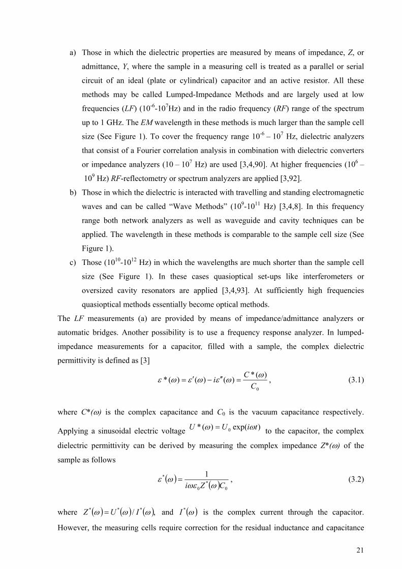
a) Those in which the dielectric properties are measured by means of impedance, Z, or
admittance, Y, where the sample in a measuring cell is treated as a parallel or serial
circuit of an ideal (plate or cylindrical) capacitor and an active resistor. All these
methods may be called Lumped-Impedance Methods and are largely used at low
frequencies (LF) (10-6-107Hz) and in the radio frequency (RF) range of the spectrum
up to 1 GHz. The EM wavelength in these methods is much larger than the sample cell
size (See Figure 1). To cover the frequency range 10-6 – 107 Hz, dielectric analyzers
that consist of a Fourier correlation analysis in combination with dielectric converters
or impedance analyzers (10 – 107 Hz) are used [3,4,90]. At higher frequencies (106 –
109 Hz) RF-reflectometry or spectrum analyzers are applied [3,92].
b) Those in which the dielectric is interacted with travelling and standing electromagnetic
waves and can be called “Wave Methods” (109-1011 Hz) [3,4,8]. In this frequency
range both network analyzers as well as waveguide and cavity techniques can be
applied. The wavelength in these methods is comparable to the sample cell size (See
Figure 1).
c) Those (1010-1012 Hz) in which the wavelengths are much shorter than the sample cell
size (See Figure 1). In these cases quasioptical set-ups like interferometers or
oversized cavity resonators are applied [3,4,93]. At sufficiently high frequencies
quasioptical methods essentially become optical methods.
The LF measurements (a) are provided by means of impedance/admittance analyzers or
automatic bridges. Another possibility is to use a frequency response analyzer. In lumped-
impedance measurements for a capacitor, filled with a sample, the complex dielectric
permittivity is defined as [3]
0
)(*)()()(*C
Ci ωωεωεωε =′′−′= , (3.1)
where C*(ω) is the complex capacitance and C0 is the vacuum capacitance respectively.
Applying a sinusoidal electric voltage )exp()(* 0 tiUU ωω = to the capacitor, the complex
dielectric permittivity can be derived by measuring the complex impedance Z*(ω) of the
sample as follows
( ) ( ) 0*
0
* 1CZi ωωε
ωε = , (3.2)
where ( ) ( ) ( ),/ *** ωωω IUZ = and ( )ω*I is the complex current through the capacitor.
However, the measuring cells require correction for the residual inductance and capacitance
21
arising from the cell itself and the connecting leads [4,94]. If a fringing field at the edges of
parallel plate electrodes causes a serious error, the three-terminal method is effective for its
elimination [95].
In general, the “Wave Methods” (b) may be classified in two ways [4,8,91,96]:
a) They may be travelling-wave or standing wave methods.
b) They may employ a guided-wave or a free–field propagation medium. Coaxial line,
metal and dielectric waveguide, microstrip line, slot line, co-planar waveguide and
optical-fiber transmission lines are examples of guided-wave media while propagation
between antennas in air uses a free-field medium.
In guided-wave propagating methods the properties of the sample cell are measured in terms
of Scattering parameters or “S-parameters” [4,97], which are the reflection and transmission
coefficients of the cell, defined in relation to a specified characteristic impedance, Z0. In
general, Z0 is the characteristic impedance of the transmission line connected to the cell (50 Ω
for most coaxial transmission lines). Note that S-parameters are complex number matrices in
the frequency domain, which describe the phase as well as the amplitude of travelling waves.
The reflection S-parameters are usually given by the symbols S*11(ω) for the multiple
reflection coefficients and S*12 for the forward multiple transmission coefficients. In the case
of single reflection S*11(ω)=ρ*(ω) the simplest formula gives the relationship between the
reflection coefficient ρ*(ω) and impedance of the sample cell terminated by a transmission
line with characteristic impedance Z0:
0
0
)(*)(*
)(*ZZZZ
+−
=ωω
ωρ
(3.3)
In all wave methods the transmission line is ideally matched except the sample holder. If the
value of Z*(ω) is differ from Z0, one can observe the reflection from a mismatch of the finite
magnitude. A similar type of wave analysis also applies in free space and in any other wave
systems, taking into account that in free space Z0≈377 Ω for plane waves.
Several comprehensive reviews on the BDS measurement technique and its application
were published [3,4,95,98] and the details of experimental tools, sample holders for solids,
powders, thin films and liquids were described there. Note that in the frequency range
10-6-3⋅1010 Hz the complex dielectric permittivity ε*(ω) can be also evaluated from the time
domain measurements of dielectric relaxation function φ(t) which is related to ε*(ω) by
(2.14). In the frequency range 10-6-105 Hz the experimental approach is simple and less time-
22
consuming than measurement in the frequency domain [3,99-102]. However, the evaluation
of complex dielectric permittivity in frequency domain requires the Fourier transform. The
details of this technique and different approaches including electrical modulus
( ) ( )ωεω ** 1=M measurements in the low frequency range were presented recently in a very
detailed review [3]. Here we will concentrate more on the time domain measurements in the
high frequency range 105-3⋅1010 Hz, usually called Time Domain Reflectometry (TDR)
methods. These will still be called TDS methods.
3.2 The Basic Principles of the TDS Methods
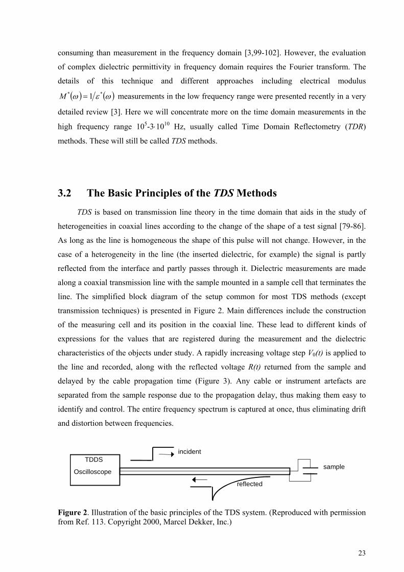
TDS is based on transmission line theory in the time domain that aids in the study of
heterogeneities in coaxial lines according to the change of the shape of a test signal [79-86].
As long as the line is homogeneous the shape of this pulse will not change. However, in the
case of a heterogeneity in the line (the inserted dielectric, for example) the signal is partly
reflected from the interface and partly passes through it. Dielectric measurements are made
along a coaxial transmission line with the sample mounted in a sample cell that terminates the
line. The simplified block diagram of the setup common for most TDS methods (except
transmission techniques) is presented in Figure 2. Main differences include the construction
of the measuring cell and its position in the coaxial line. These lead to different kinds of
expressions for the values that are registered during the measurement and the dielectric
characteristics of the objects under study. A rapidly increasing voltage step V0(t) is applied to
the line and recorded, along with the reflected voltage R(t) returned from the sample and
delayed by the cable propagation time (Figure 3). Any cable or instrument artefacts are
separated from the sample response due to the propagation delay, thus making them easy to
identify and control. The entire frequency spectrum is captured at once, thus eliminating drift
and distortion between frequencies.
incident
reflected
sample TDDS
Oscilloscope
Figure 2. Illustration of the basic principles of the TDS system. (Reproduced with permission from Ref. 113. Copyright 2000, Marcel Dekker, Inc.)
23

Figure 3. Characteristic shape of the signals recorded during a TDS experiment, V0(t), incident pulse; R(t), reflected signal. (Reproduced with permission from Ref. 86. Copyright 1996, American Institute of Physics.)
The complex permittivity is obtained as follows: For non-disperse materials (frequency-
independent permittivity), the reflected signal follows the exponential response of the RC
line-cell arrangement; for disperse materials, the signal follows a convolution of the line-cell
response with the frequency response of the sample. The actual sample response is found by
writing the total voltage across the sample as follows
)()()( 0 tRtVtV += , (3.4)
and the total current through the sample [80,86,103]
( ) ( ) ( )[ ]tRtVtI −= 00Z
1
, (3.5)
where the sign change indicates direction and Z0 is the characteristic line impedance. The total
current through a conducting dielectric is composed of the displacement current , and the
low-frequency current between the capacitor electrodes
( )tI D
( )tI R . Since the active resistance at
zero frequency of the sample-containing cell is [86] (Figure 3):
( )( )
( ) ( )( ) ( )tRtV
tRtVZtItVr
tt −+
==∞→∞→
0
00 limlim
, (3.6)
the low-frequency current can be expressed as:
( ) ( ) ( ) ( ) ( ) ( )( ) ( )tRtV
tRtVZ
tRtVrtVtI
tR +−+
==∞→
0
0
0
0 lim
(3.7)
Thus relation (3.5) can be written as:
24
[ ] [ ]⎭⎬⎫
⎩⎨⎧
+−
+−−=∞→ )()(
)()()()()()(1)(0
000
0 tRtVtRtV
limtRtVtRtVZ
tIt
D
(3.8)
Relations (3.4) and (3.8) present the basic equations that relate I(t) and V(t) to the signals
recorded during the experiment. In addition, (3.8) shows that TDS permits one to determine
the low-frequency conductivity σ of the sample directly in time domain [84-86]:
( ) ( )( ) ( )tRtV
tRtVlimCZ t +
−ε=σ
∞→0
0
00
0
(3.9)
Using I(t),V(t) or their complex Fourier transforms i(ω) and v(ω) one can deduce the relations
that will describe the dielectric characteristics of a sample being tested either in frequency or
time domain. The final form of these relations depends on the geometric configuration of the
sample cell and its equivalent representation [79-86].
The admittance of the sample cell terminated to the coaxial line is then given by
( ) ( )( )ωω
=ωΥvi
, (3.10)
and the sample permittivity can be presented as follows:
( ) ( )0
YCiωω
=ωε .
(3.11)
To minimize line artefacts and establish a common time reference, (3.10) is usually rewritten
in differential form, to compare reflected signals from the sample and a calibrated reference
standard and thus eliminate V0(t) [79-86].
If one takes into account the definite physical length of the sample and multiple
reflections from the air-dielectric or dielectric-air interfaces, relation (3.11) must be written in
the following form [79-84,103]:
( ) ( ) ( ) XXYdi
c cotωγω
=ωε∗
, (3.12)
where )()c/d(X * ωεω= , d is the length of the inner conductor, c is the velocity of light,
and γ is the ratio between the capacitance per unit length of the cell to that of the matched
coaxial cable. Equation (3.12) in contrast to (3.11) is a transcendental one, and its exact
solution can be obtained only numerically [79-84]. The key advantage of TDS methods in
25

comparison with frequency methods is the ability to obtain the relaxation characteristics of a
sample directly in time domain. Solving the integral equation one can evaluate the results in
terms of the dielectric response function Φ(t) [86,103,104]. It is then possible to associate
with the macroscopic dipole correlation function Ψ(t) [2,105,106] in the
framework of linear response theory.
( ) ( ) ∞ε+Φ=ϕ tt
3.2.1
Experimental Tools
3.2.1.1 Hardware
The standard time-domain reflectometers used to measure the inhomogeneities of coaxial
lines [80, 86,107,108] are the basis of the majority of modern TDS-setups. The reflectometer
consists of a high-speed voltage step generator and a wide-band registering system with a
single or double-channel sampling head. In order to meet the high requirements of TDS
measurements such commercial equipment must be considerably improved. The main
problem is due to the fact that the registration of incident V(t) and reflected R(t) signals is
accomplished by several measurements. In order to enhance the signal - noise ratio one must
accumulate all the registered signals. The high level of drift and instabilities during generation
of the signal and its detection in the sampler are usually inherent to the serial reflectometry
equipment.
The new generation of digital sampling oscilloscopes [109-111] and specially designed
time domain measuring set-ups [86] offer comprehensive, high precision, and automatic
measuring systems for TDS hardware support. They usually have a small jitter-factor (< 1.5
ps), important for rise time; small flatness of incident pulse (<0.5 % for all amplitudes) and in
some systems a unique option for parallel time non-uniform sampling of the signal [86].
The typical TDS set-up consists of a signal recorder, a 2-channel sampler and a built-in
pulse generator. The generator produces 200 mV pulses of 10 μs duration and short rise time
(~30 ps). Two sampler channels are characterized by an 18 GHz bandwidth and 1.5 mV noise
(RMS). Both channels are triggered by one common sampling generator that provides their
time correspondence during operation. The form of the voltage pulse thus measured is
digitized and averaged by the digitizing block of Time Domain Measurement System
(TDMS). The time base is responsible for the major metrology TDMS parameters. The block
diagram of the described TDS set-up is presented in Figure (4) [86].
26

A B
Control Unit
USB (Main Frame)
Sample
Sampling head with built in generator
Figure 4. Circuit diagram of a TDS setup. Here A and B are two sampler channels.
3.2.1.2 Non-uniform Sampling
In highly disordered complex materials, the reflected signal R(t) extends over wide ranges of
time and cannot be captured on a single time scale with adequate resolution and sampling
time. In an important modification of regular TDR systems, a non-uniform sampling
technique (parallel or series), has been developed [86,112].
In the series realization consecutive segments of the reflected signal on an increasing
time scale are registered and linked into a combined time scale. The combined response is
then transformed using a running Laplace transform to produce the broad frequency spectra
[112].
In the parallel realization a multi-window sampling time scale is created [86]. The
implemented time scale is the piecewise approximation of the logarithmic scale. It includes
nw⊆16 sites with a uniform discretization step determined by the following formula:
nwnw 21 ×δ=δ , (3.13)
where δ1=5 ps is the discretization step at the first site, and the number of points in each step
except for the first one is equal to npw=32. At the first site, the number of points
npw1=2*npw. The doubling of the number of points at the first site is necessary in order to
have the formal zero time position, which is impossible in the case of the strictly logarithmic
structure of the scale. In addition, a certain number of points located in front of the zero time
position are added. They serve exclusively for the visual estimation of the stability of the time
position of a signal and are not used for the data processing.
27
The described structure of the time scale allows the overlapping of the time range from
5 ps to 10 μs during one measurement, which results in a limited number of registered
readings. The overlapped range can be shortened, resulting in a decreasing number of
registered points and thus reducing the time required for data recording and processing.
The major advantage of the multi-window time scale is the ability to get more
comprehensive information. The signals received by using such a scale contain information
within a very wide time range and the user merely decides which portion of this information
to use for further data processing. Also, this scale provides for the filtration of registered
signals close to the optimal one already at the stage of recording.
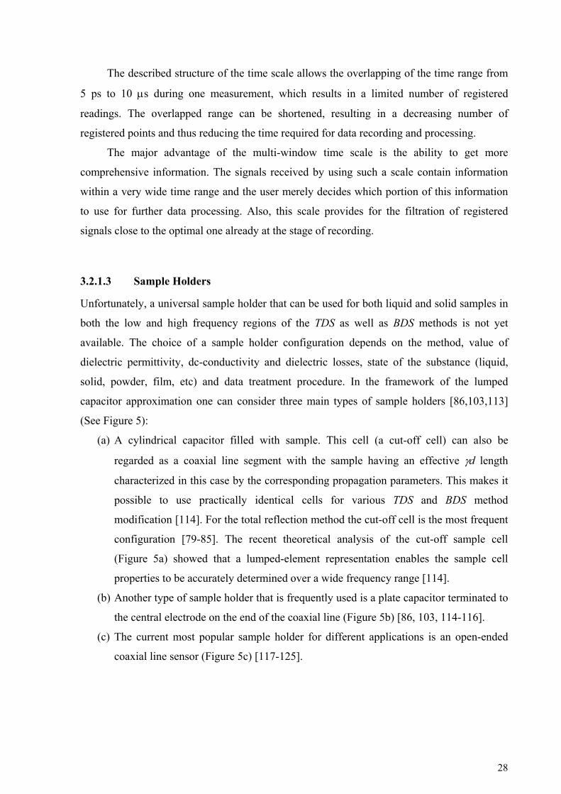
3.2.1.3 Sample Holders
Unfortunately, a universal sample holder that can be used for both liquid and solid samples in
both the low and high frequency regions of the TDS as well as BDS methods is not yet
available. The choice of a sample holder configuration depends on the method, value of
dielectric permittivity, dc-conductivity and dielectric losses, state of the substance (liquid,
solid, powder, film, etc) and data treatment procedure. In the framework of the lumped
capacitor approximation one can consider three main types of sample holders [86,103,113]
(See Figure 5):
(a) A cylindrical capacitor filled with sample. This cell (a cut-off cell) can also be
regarded as a coaxial line segment with the sample having an effective γd length
characterized in this case by the corresponding propagation parameters. This makes it
possible to use practically identical cells for various TDS and BDS method
modification [114]. For the total reflection method the cut-off cell is the most frequent
configuration [79-85]. The recent theoretical analysis of the cut-off sample cell
(Figure 5a) showed that a lumped-element representation enables the sample cell
properties to be accurately determined over a wide frequency range [114].
(b) Another type of sample holder that is frequently used is a plate capacitor terminated to
the central electrode on the end of the coaxial line (Figure 5b) [86, 103, 114-116].
(c) The current most popular sample holder for different applications is an open-ended
coaxial line sensor (Figure 5c) [117-125].
28

Figure 5. Simplified drawings of sample cells. (a) Open coaxial line cell; (b) lumped capacitance cell; (c) open-ended coaxial cell. (Reproduced with permission from Ref. 113. Copyright 2000, Marcel Dekker, Inc.)
(c)(a) (b)
Teflon Sample
In the case of lumped capacitance approximation the configurations in (See Figures 5a-b)
have high frequency limitations and for highly polar systems one must take into account the
finite propagation velocity of the incident pulse [82-86,113]. The choice of sample cell shape
is determined to a high extent by the aggregate condition of the system under study. While
cell (a) is convenient to measure liquids, configuration (b) is more suitable for the study of
solid disks, crystals [115,126] and films. Both cell types can be used to measure powder
samples. While studying anisotropic systems (liquid crystals, for instance) the user may
replace a coaxial line by a strip line or construct the cell with the configuration providing
measurements under various directions of the applied electric field [84,85]. The (c) type cell
is used only when it is impossible to put the sample into the (a) or (b) cell types [86,121-
125,127-129]. The fringing capacity of the coaxial line end is the working capacity for such a
cell. This kind of cell is widely used now for investigating the dielectric properties of
biological materials and tissues [122-125], petroleum products [119], constructive materials
[110], soil [129] and numerous other non-destructive permittivity and permeability
measurements. Theory and calibration procedures for such open-coaxial probes are well
developed [129-131] and the results meet the high standards of other modern measuring
systems.
29
3.2.2
3.3.1
Data Processing
Measurement procedures, registration, storage, time referencing and data analyses are
carried out automatically in the modern TDS systems. The process of operation is performed
in an on-line mode and the results can be presented in both frequency and time domain [86].
There are several features of the modern software that control the process of measurement and
calibration. One can define the time windows of interest that may be overlapped by one
measurement. During the calibration procedure the precise determination of the front edge
position is carried out and the setting of an internal auto centre on these positions applies to
all subsequent measurements. The precise determination and settings of horizontal and
vertical positions of calibration signals are also carried out. All parameters may be saved in a
configuration file, allowing for a complete set of measurements using the same parameters
without additional calibration.
The data processing software includes the options of signal correction, correction of
electrode polarization and dc-conductivity, and different fitting procedures both in time and
frequency domain [86].
3.3 Data analysis and fitting problems
The principle difference between the BDS and TDS methods is that BDS
measurements are fulfilled directly in frequency domain while the TDS operates in time
domain. In order to avoid unnecessary data transformation it is preferable to perform data
analysis directly in the domain, where the results were measured. However, nowadays there
are no principle difficulties to transform data from one domain to another by direct or inverse
Fourier transform. Below we will concentrate on the details of data analysis only in the
frequency domain.
The continuous parameter estimation problem
Dielectric relaxation of complex materials over wide frequency and temperature
ranges in general may be described in terms of several non-Debye relaxation processes. A
quantitative analysis of the dielectric spectra begins with the construction of a fitting function
in selected frequency and temperature intervals, which corresponds to the relaxation processes
in the spectra. This fitting function is a linear superposition of the model functions (such as
HN, Jonscher, dc-conductivity terms, See Paragraph 2.2.1) that describes the frequency
30
dependence of the isothermal data of the complex dielectric permittivity. The temperature
behavior of the fitting parameters reflects the structural and dynamic properties of the
material.
However, there are several problems in selecting the proper fitting function, such as
the limited frequency and temperature ranges of the experiment, distortion influences of the
sample holder and the overlapping of several physical processes with different amplitudes in
the same frequency and temperature ranges. The latter is the most crucial problem, because
some of the relaxation processes are “screened” by the others. For such a “screened” process,
the confidence in parameter estimations can be very small. In this case, the temperature
functional behavior of the parameters may be inconsistent. Despite these discontinuities, there
may still be some trends in the parameter behavior of the “screened” processes which may
reflect some tendencies of the physical processes in the system. Therefore, it is desirable to
obtain a continuous solution of the model parameters via temperature. This solution is hardly
achievable if the estimation of the parameters is performed independently for the different
temperature points on the selected fitted range. Post-fitted parameter smoothing can spoil the
quality of the fit. A new procedure for smooth parameter estimation, named the “global fit”,
was proposed recently [132]. It obtains a continuous solution for the parameter estimation
problem. In this approach, the fitting is performed simultaneously for all the temperature
points. The smoothness of the solution is obtained by the addition of some penalty term to the
cost function in the parameter minimization problem. Coupled with a constraint condition for
the total discrepancy measure between the data and the fit function [132], the desired result is
achieved.
The penalized functional approach for obtaining a continuous solution of the
minimization problem is a well-known regularization technique in image restoration problems
such as image de-noising or image de-blurring [133].
In the field of dielectric spectroscopy such regularization procedures have been used
by Schäfer et al. [14] for extracting the logarithmic distribution function of relaxation times,
G(τ). In contrast to the parametric description of the broadband dielectric spectra considered
in our work, the approach of Schäfer et al is essentially non-parametric. These authors used a
regularization technique for the construction of the response function through the Fredholm
integral equation solution. The approach proposed in [132] deals with the problem of finding
fitting parameters that describe dielectric data in the frequency domain in a wide frequency
band, to obtain a continuous estimation of the fitting parameters via temperature, or any other
external parameters.
31

3.3.2 dc-Сonductivity problems
The dielectric spectroscopy study of conductive samples is very complicated because
of the need to take into account the effect of dc-conductivity. The dc-conductivity 0σ
contributes, in frequency domain, to the imaginary part of the complex dielectric permittivity
as an additional function 0 0/( )σ ε ω . The presence of dc-conductivity makes it difficult to
analyze relaxation processes especially when the contribution of the conductivity is much
greater than the amplitude of the process. The correct calculation of the dc-conductivity is
important in terms of the subsequent analysis of the dielectric data. Its evaluation by fitting of
the experimental data does not always give correct results, especially when relaxation
processes are present in the low frequency range. In particular, the dc-conductivity function
has frequency power-law dependence similar to the Jonscher terms in the imaginary part of
the complex dielectric permittivity and this makes computation of dc-conductivity even more
difficult.
It is known that in some cases the modulus representation M*(ω) of dielectric data is
more efficient for dc-conductivity analysis, since it changes the power law behavior of the
dc-conductivity into a clearly defined peak [134]. However, there is no significant advantage
of the modulus representation when the relaxation process peak overlaps the conductivity
peak. Moreover, the shape and position of the relaxation peak will then depend on the
conductivity. In such a situation, the real component of the modulus, containing the
dc-conductivity as an integral part, does not help to distinguish between different relaxation
processes.
Luckily, the real and imaginary parts of the complex dielectric permittivity are not
independent of each other and are connected by means of the Kramers–Kronig relations [11].
This is one of the most commonly encountered cases of dispersion relations in linear physical
systems. The mathematical technique used by the Kramers–Kronig relations is the Hilbert
transform. Since dc-conductivity enters only the imaginary component of the complex
dielectric permittivity the static conductivity can be calculated directly from the data by
means of the Hilbert transform.
32

3.3.3 Continuous Parameter Estimation Routine
The complex dielectric permittivity data of a sample, obtained from DS measurements in a
frequency and temperature interval can be organized into the matrix data massive ,i jε⎡ ⎤≡ ⎣ ⎦ε of
size M N× , where , ( , )i j i jTε ε ω≡ , M is the number of measured frequency points and is
the number of measured temperature points. Let us denote by
N
( ; )f f ω= x the fitting function
of n parameters 1 2{ , ,..., }nx x x
( ; (
=x . This function is assumed to be a linear superposition of the
model descriptions (such as the Havriliak-Negami function or the Jonscher function,
considered in section 2.2.1). The dependence of f on temperature T can be considered to be
via parameters only: ))f f Tω= x . Let us denote by ( )i jX x T⎡ ⎤≡ ⎣ ⎦
jT
the n matrix of n
model parameters xi , computed at N different temperature points .
N×
The classical approach to the fit parameter estimation problem in dielectric
spectroscopy is generally formulated in terms of a minimization problem: finding values of X
which minimize some discrepancy measure between the measured values, collected in
the matrix ε and the fitted values of the complex dielectric permittivity.
The choice of depends on noise statistics [132].
( , )S ε ε$
, (if ω x[ ( ))]jT=ε$
( , )S ε ε$
3.3.4 Computation of the dc-conductivity using Hilbert transform
The coupling between real and imaginary components of the complex dielectric
permittivity )(* ωε is provided by the Kramers-Kronig relations, one of the most general
cases of dispersion relations in physical systems. The mathematical technique used by the
Kramers-Kronig relations, which allows one component to be defined through another, is the
Hilbert transform since '( )ε ω and ''( )ε ω are Hilbert transform pairs. Performing a Hilbert
transform of '( )ε ω and subtracting the result from ''( )ε ω , the dc-conductivity, 0 0/( )σ ε ω , can
be computed directly from the complex dielectric permittivity data. The simulated and
experimental examples show very good accuracy for calculating dc-conductivity by this
method.
The Kramers-Kronig dispersion relations between imaginary and real parts of
dielectric permittivity can be written as follows [11]:
33

( ) ( ) ωωω
ωεπ
εωε ′−′
′′′+=′ ∫
∞
∞−∞ dP
ˆˆ1
, (3.14)
( ) ( ) ( ) ωωω
ωεπωε
σωεωε ′−′
′′=−′′=′′ ∫
∞
∞−
dP1ˆ0
0
, (3.15)
where the symbol P denotes the Cauchy principal value of the integral. The Hilbert transform
of a real function is defined as: [ ]H g ( )g t
1 ( )[ ] gH g P dξ ξπ ξ ω
∞
−∞
= −−∫
(3.16)
Therefore the conductivity term in the second dispersion relation (3.15) can be presented as
follows:
( ) ( )ωεωεωε
σ ˆ0
0 ′′−′′= .
(3.17)
The result shows that dc-conductivity can be computed by using the Hilbert transform
applied to the real components of the dielectric permittivity function and subtracting the result
from its imaginary components. The main obstacle to the practical application of the Hilbert
transform is that the integration in equation (3.16) is performed over infinite limits; however,
a DS spectroscopy measurement provides values of )(* ωε only over some finite frequency
range. Truncation of the integration in the computation of the Hilbert Transform can yield a
serious computational error in calculating [ ])(ωε ′H in the measured frequency range. This
problem cannot be overcome unless the “missing” dielectric data is supplied. However, the
computational error can be reduced by extending '( )ε ω
4
into a frequency domain outside the
measuring frequency range. Although this is a rather crude data treatment, computer
simulations show that computational error due to the truncation of the measuring frequency
range is greater near the borders of the range. Far from the borders of the frequency range the
relative error is much smaller and is of the order of 10− .
While our method works well with most situations, it is limited when '( )ε ω exhibits a
low frequency tail. Such a situation is characteristic of percolation, electrode polarization or
other low-frequency process, where the reciprocal of the characteristic relaxation time for the
process is just below our frequency window. In this case aliasing effects distort the transform
result.
34

Practically, the Numerical Hilbert Transform can be computed by means of the well-
known Fast Fourier Transform (FFT) routine. It is based on the following property of the
Hilbert Transform [135]. If
[0
1( ) ( )cos ( )sing t a t b t d]ω ω ω ωπ
∞
= +∫ ω
(3.18)
is the Fourier transform of a real function , then the Fourier-transform of the function
is the following:
( )g t
[ ]H g
[0
1[ ] ( )cos ( )sinH g b t a t d]ω ω ω ωπ
∞
= −∫ ω
3.3.5
. (3.19)
Thus, by performing the Fourier transform of the data with an FFT algorithm, the Hilbert
transform is computed by inverse-FFT operation to the phase-shifting version of the Fourier
transform of the original data. Such an approach was realized in the work of Castro and Nabet
[136], where the real component of the dielectric permittivity was calculated from its
imaginary component, using the Hilbert transform. For the Hilbert transform computation, the
authors used a procedure included in the MATLAB package. This methodology was also
based on the FFT technique, requiring uniform sampling over the frequency interval. If the
data are not measured uniformly, it should be interpolated to frequency points, evenly spaced
with an incremental frequency equal to or less than the start frequency. However, this routine
cannot be used for a wide spectral range. For example, in order to cover an interval of 12
decades with an incremental frequency equal to the start frequency 1012 points are required.
This, of course, is not practical. To overcome this limitation, a procedure based on a moving
frequency window has been developed, where the scale inside the window is linear, but the
window jump is logarithmic. This kind of methodology employing moving windows with
FFT has been used in the past [137].
Computing software for data analysis and modeling
Software for dielectric data treatment and modeling in frequency domain has been
developed recently [132]. This program (MATFIT) was built around the software package
MATLAB (Math Works Inc.) and its functionality is available through an intuitive visual
interface. Key features of the program include:
35

• Advanced data visualization and pre-processing tools for displaying complex dielectric
permittivity data and selecting appropriate frequency and temperature intervals for modeling;
• A library of standard relaxation fit functions;
• Simultaneous fit of both real and imaginary components of the complex dielectric
permittivity data;
• Linear and nonlinear fitting methods, from least-squares and logarithmic to fitting
procedures based on the entropy norm;
• Global fit procedure on all selected temperature ranges for continuous parameter estimation;
• Hilbert transform for computing dc-conductivity;
• Parameter visualization tool for displaying fitting parameter functions via temperature and
subsequent analysis of the graphs.
The methodology described above, utilized in the presented program [132], and
reduces the problem of dielectric data analysis to choosing the appropriate model functions
and an estimation of their model parameters. The penalized maximum likelihood approach for
obtaining these parameters as a function of temperature has proven to be a consistent method
for accurately obtaining the global minimum in this estimation. This methodology is a
phenomenological approach to obtaining the underlying temperature dependence of the
parameter space, while not presupposing a particular physical model. The risk is present that
such a regularization routine may perturb the result if used excessively. For this reason a
regularization parameter is used to control the smoothing term. However, this risk is far less
than the risk of a priori conclusion of the result according to the researcher’s personal belief
in a preferred analytical model.
4 Dielectric response in some disordered materials In this contribution we are presenting some concepts of modern dielectric
spectroscopy. We are going to illustrate these ideas by experimental examples related to
different complex systems. In many cases we will refer different features of dielectric
response observed in the same samples. Parallel with the description of morphology for each
system, the phenomenological identification of the relaxation processes and their relation to
dynamic of structural units is established. In spite of the structural and dynamic differences,
the general features of the relaxation processes will be indicated.
36

4.1 Microemulsions
Microemulsions are thermodynamically stable, clear fluids, composed of oil, water,
surfactant and sometimes co-surfactant that have been widely investigated during recent years
because of their numerous practical applications. The chemical structure of surfactants may be
low-molecular weight as well as polymeric, with nonionic or ionic components [138-141]. In
the case of a water/oil-continuous (W/O) microemulsion, at low concentration of the
dispersed phase, the structure is that of spherical water droplets surrounded by a
monomolecular layer of surfactant molecules whose hydrophobic tails are oriented towards
the continuous oil phase (See Figure 6). When the volume fractions of oil and water are high
and comparable, random bicontinuous structures are expected to form.
Figure 6. Schematic presentation of spherical water droplet surrounded by a monomolecular layer of ionic surfactant molecules.
The structure of the microemulsion depends on the interaction between droplets. In the
case of repulsive interaction, the collisions of the droplets are short and no overlapping occurs
between their interfaces. However, if the interactions are attractive, transient random droplet
clusters are formed. The number and sizes of such clusters are increasing with the
temperature, the pressure, or the water to surfactant ratio, leading to a percolation in the
system [113,142-145].
The majority of the different chemical and physical properties, as well as the
morphology of microemulsions, is determined mostly by the micro-Brownian motions of its
components. Such motions cover a very wide spectrum of relaxation times ranging from tens
of seconds to a few picoseconds. Given the complexity of the chemical makeup of
microemulsions, there are many various kinetic units in the system. Depending on their
nature, the dynamic processes in the microemulsions can be classified into three types:
37
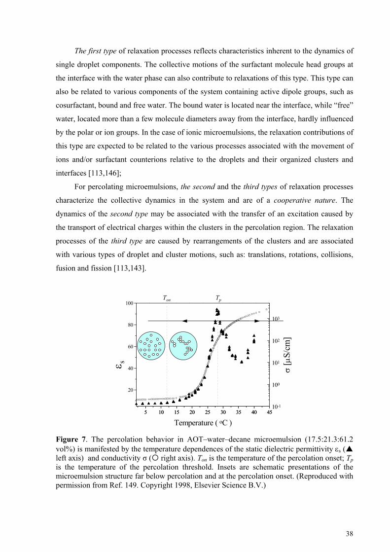
The first type of relaxation processes reflects characteristics inherent to the dynamics of
single droplet components. The collective motions of the surfactant molecule head groups at
the interface with the water phase can also contribute to relaxations of this type. This type can
also be related to various components of the system containing active dipole groups, such as
cosurfactant, bound and free water. The bound water is located near the interface, while “free”
water, located more than a few molecule diameters away from the interface, hardly influenced
by the polar or ion groups. In the case of ionic microemulsions, the relaxation contributions of
this type are expected to be related to the various processes associated with the movement of
ions and/or surfactant counterions relative to the droplets and their organized clusters and
interfaces [113,146];
For percolating microemulsions, the second and the third types of relaxation processes
characterize the collective dynamics in the system and are of a cooperative nature. The
dynamics of the second type may be associated with the transfer of an excitation caused by
the transport of electrical charges within the clusters in the percolation region. The relaxation
processes of the third type are caused by rearrangements of the clusters and are associated
with various types of droplet and cluster motions, such as: translations, rotations, collisions,
fusion and fission [113,143].
5 10 15 20 25 30 35 40 45
ε s
Temperature ( oC )
0 2 4 6 8 10
10-1
100
101
102
103
σ [μ
S/cm
]
5 10 15 20 25 30 35 40 45
20
40
60
80
100TpTon
ε s
Figure 7. The percolation behavior in AOT–water–decane microemulsion (17.5:21.3:61.2 vol%) is manifested by the temperature dependences of the static dielectric permittivity εs ( left axis) and conductivity σ ( right axis). Ton is the temperature of the percolation onset; Tp is the temperature of the percolation threshold. Insets are schematic presentations of the microemulsion structure far below percolation and at the percolation onset. (Reproduced with permission from Ref. 149. Copyright 1998, Elsevier Science B.V.)
38

Dielectric Spectroscopy can be successful in providing unique information about the
dynamics and structure of microemulsions on various spatial and temporal scales. Being
sensitive to percolation, DS is expected to provide unambiguous conclusions concerning the
stochastic type, the long time scale cooperative dynamics and the imposed geometric
restrictions of molecular motions before, during and after the percolation threshold in
microemulsions. It also can give valuable information about fractal dimensions and sizes of
the percolation clusters.
The percolation behavior is manifested by the rapid increase in the dc-electrical
conductivity σ and the static dielectric permittivity εs as the system approaches the
percolation threshold (Figure 7).
The dielectric relaxation properties in a sodium bis(2-ethylhexyl) sulfosuccinate (AOT) -
water - decane microemulsion near the percolation temperature threshold have been
investigated in a broad temperature region [47,143,147]. The dielectric measurements of ionic
microemulsions were carried out using the TDS in a time window with a total time interval of
~ 1μs. It was found that the system exhibits a complex non-exponential relaxation behavior
that is strongly temperature dependent (Figure 8).
An interpretation of the results was done in the framework of the dynamic percolation
model [148]. According to this model, near the percolation threshold, in addition to the fast
relaxation related to the dynamics of droplet components (τ1 ≅ 1 ns) [149], there are at least
Figure 8. Three-dimensional plots of the frequency and temperature dependence of the dielectric permittivity ε′ (a) and dielectric losses ε″ (b) for AOT–water–decane microemulsion. (Reproduced with permission from Ref. 143. Copyright 1995, The American Physical Society.)
39

two much longer characteristic time scales. The longest process has a characteristic relaxation
time greater than a few microseconds and is associated with the rearrangement of the typical
percolation cluster. The temporal window of the intermediate process is a function of
temperature. This intermediate process reflects the cooperative relaxation phenomenon
associated with the transport of charge carriers along the percolation cluster [148,150,151].
Thus, due to the cooperative nature of relaxation, the DCF decay behavior (See Figure 9)
contains information regarding the transient cluster morphology at the mesoscale that reflects
the dynamical character of percolation.
Figure 9. The three-dimensional plot of experimental dipole correlation function versus time and temperature. The percolation threshold temperature Tp=26.5°C. (Reproduced with permission from Ref. 47. Copyright 1996, The American Physical Society.)
The type of the relaxation law seen in time domain is strongly dependent on the
distance from the percolation threshold. Figure 10 shows in log-log coordinates that at the
percolation onset temperature (~14°C) the relaxation follows a fractional power law:
Ψ(t) ~ (t/τ1)−μ. By the same token, in the coordinates logΨ versus log(t/τ1) in the close
vicinity of the percolation threshold Tp=26.5°C, the relaxation law changes from power law to
stretched exponential behavior, i.e., Ψ(t) ~ exp[-(t/τm)ν] (See Figure 11). In the crossover
region the relaxation law is considered to be a product of both the power law and stretched
exponential terms described by (2.25). The results of the fitting of the experimental dipole
correlation functions to Eq.(2.25) are shown in Figure 12 and Figure 13.
One can see (Figure 12) that the magnitude of parameter μ decreases to almost zero as
the temperature approaches that of the percolation threshold. This effect confirms the
statement mentioned above that at the percolation threshold temperature the behavior of the
40

dipole correlation function is of the KWW type. The stretched parameter ν changes its value
from ~0.2 near the percolation onset to ∼0.8 in the vicinity of the percolation threshold.
Figure 10. The dipole correlation function ψ (t/τ1) demonstrates power-law behavior for the temperature region near the percolation onset (Ton = 12°C). (Reproduced with permission from Ref. 2. Copyright 2002, Elsevier Science B.V.)
Figure 11. The dipole correlation function ψ (t/τ1) demonstrates KWW behaviour near the temperature of the percolation threshold (Tp = 26.5°C). (Reproduced with permission from Ref. 2. Copyright 2002, Elsevier Science B.V.)
Figure 12. The temperature dependence of the exponents μ (▼) and ν (■) illustrate the transformation of the dipole correlation function ψ (t/τ1) from the power-law pattern to the KWW behavior at the percolation threshold. (Reproduced with permission from Ref. 2. Copyright 2002, Elsevier Science B.V.)
Figure 13. The temperature dependence of the parameter τm (● left axis) and A (▲ right axis), obtained by the fitting of the relaxation law (25) to the experimental data. (Reproduced with permission from Ref. 2. Copyright 2002, Elsevier Science B.V.)
41
Notwithstanding that the value of ν is not equal to zero at percolation onset, note that the
stretched exponential term with ν = 0.2 changes insignificantly in the considerable time
interval (~1μs) and the decay of the DCF ψ(t) is governed mainly by the power law. Figure
13 plots the relaxation times ratio, τm / τ1 and the amplitude A corresponding to the
macroscopic relaxation time of the decay function determined by (2.25). Near the percolation
threshold, τm / τ1 exhibit a maximum and reflect the well-known critical slowing down effect
[152]. The description of the mechanism of the cooperative relaxation in the percolation
region will be presented in section 5.2.
4.2 Porous materials
Non-Debye dielectric relaxation in porous systems is another example of the dynamic
behavior of complex systems on a mesoscale. The dielectric properties of various complex
multi-phase systems (borosilicate porous glasses [153-156], sol-gel glasses [157,158],
zeolites [159] and porous silicon [160,161]) were studied and analyzed in terms of
cooperative dynamics. The dielectric response in porous systems will be considered here in
detail using two quite different types of the materials namely: porous glasses and porous
silicon.
4.2.1 Porous glasses
The porous silica glasses obtained from sodium borosilicate glasses are defined as
bicontinuous random structures of two interpenetrating percolating phases, the solid and the
pore networks. The pores in the glasses are connected to each other and the pore size
distribution is narrow. The characteristic pore spacing depends on the method of preparation,
and can be between 2 and 500 nm [156,162]. A rigid SiO2 matrix represents the irregular
structure of porous glasses. Water can be easily adsorbed on the surface of this matrix. The
dielectric relaxation properties of two types of silica glasses have been studied intensively
over broad frequency and temperature ranges [153-156]. The typical spectra of the dielectric
permittivity and losses associated with the relaxation of water molecules of the adsorptive
layer for the studied porous glasses versus frequency and temperature are displayed in Figure
14.
42

Figure 14 shows that the complex dielectric behavior can be described in terms of the four
distributed relaxation processes as follows:
The first relaxation process, which is observed in the low temperature region from –100°C
to +10°C is due to the reorientation of the water molecules in ice-like water cluster structures.
It was shown that the hindered dynamics of the water molecules located within the pores
reflects the interaction of the absorptive layer with the inner surfaces of the porous matrix
[153,155];
The second relaxation process has a specific saddle-like shape and is well marked in the
temperature range of –50°C to +150°C. This relaxation process is thought to be a kinetic
transition due to water molecule reorientation in the vicinity of a defect [155];
Figure 14. The typical three-dimensional plot of the complex dielectric permittivity real ε′ (a) and imaginary part ε″ (b) versus frequency and temperature for porous glass (sample E). All the details of different sample preparation and their properties are presented in Ref. 156. (Reproduced with permission from Ref. 2. Copyright 2002, Elsevier Science B.V.)
The third relaxation process is located in the low-frequency region and the temperature
interval 50°C to 100°C. The amplitude of this process essentially decreases when the
frequency increases, and the maximum of the dielectric permittivity versus temperature has
almost no temperature dependence (Figure 15). Finally, the low-frequency ac-conductivity σ
demonstrates an S-shape dependency with increasing temperature (Fig. 16), which is typical
of percolation [2,143,154]. Note in this regard that at the lowest-frequency limit of the
covered frequency band the ac-conductivity can be associated with dc-conductivity σ0 usually
measured at a fixed frequency by traditional conductometry. The dielectric relaxation process
here is due to percolation of the apparent dipole moment excitation within the developed
43
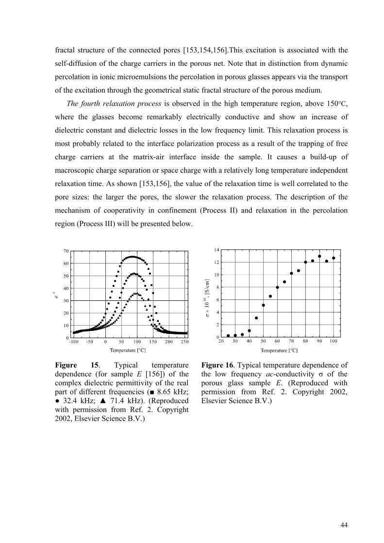
fractal structure of the connected pores [153,154,156].This excitation is associated with the
self-diffusion of the charge carriers in the porous net. Note that in distinction from dynamic
percolation in ionic microemulsions the percolation in porous glasses appears via the transport
of the excitation through the geometrical static fractal structure of the porous medium.
The fourth relaxation process is observed in the high temperature region, above 150°C,
where the glasses become remarkably electrically conductive and show an increase of
dielectric constant and dielectric losses in the low frequency limit. This relaxation process is
most probably related to the interface polarization process as a result of the trapping of free
charge carriers at the matrix-air interface inside the sample. It causes a build-up of
macroscopic charge separation or space charge with a relatively long temperature independent
relaxation time. As shown [153,156], the value of the relaxation time is well correlated to the
pore sizes: the larger the pores, the slower the relaxation process. The description of the
mechanism of cooperativity in confinement (Process II) and relaxation in the percolation
region (Process III) will be presented below.
Figure 15. Typical temperature dependence (for sample E [156]) of the complex dielectric permittivity of the real part of different frequencies (■ 8.65 kHz; ● 32.4 kHz; ▲ 71.4 kHz). (Reproduced with permission from Ref. 2. Copyright 2002, Elsevier Science B.V.)
Figure 16. Typical temperature dependence of the low frequency ac-conductivity σ of the porous glass sample E. (Reproduced with permission from Ref. 2. Copyright 2002, Elsevier Science B.V.)
44

4.2.2 Porous Silicon
Non-Debye dielectric relaxation was also observed in porous silicon (PS) [25,
160,161]. PS has attracted much attention, mainly due to its interesting optical and electro-
optical properties that can be utilized for device applications [164,165]. So far, most of the
activity in this field has focused on the intense visible photoluminescence (PL) from nano-PS
and the underlying physical mechanism that is responsible for the generation of light. In
addition, transport and dielectric relaxation phenomena in PS have also attracted considerable
attention for injection-type PS devices. It was mentioned in the previous section that the
correlation between the morphology of porous media and their dielectric properties has
already been studied [153,154,166]. In many porous media, dielectric response is directly
related to the fractality and the nano- and meso-structural properties of these disordered
systems [153,156-159]. In principle, one would expect to find a similar correlation between
the micro-geometry and the dielectric properties of PS media. For example, dc-conductivity
measurements demonstrate a dual transport mechanism that has been assigned to thermally
activated hopping and exited charged carrier tunneling [167]. As a result, carriers excited to
the band tail would give rise to a thermally activated dc-conduction with activation energy of
about 0.5 eV [163,168]. This activation energy is less than half the optical band-gap of PS
deduced from PL experiments [164]. The ac-conductivity measurements in PS revealed
complex transport properties due to a random walk in fractal geometry and thermally
activated hopping, as in the case of dc-conductivity [163]. Therefore, it is commonly accepted
that both the nano-geometry, the nature of the Si nanocrystallites that form the PS medium
and their surfaces as well as the host matrix all contribute to the electrical and optical
properties of PS.
The dielectric relaxation properties in nano-PS with different thicknesses have been
investigated in broad frequency and temperature regions [160,161]. The dielectric properties
of the PS samples were measured in the 20 Hz to 1MHz frequency range and in the
173 to 493 K temperature interval. For all the dielectric measurements, the amplitude of a
sinusoidal ac voltage source was kept constant at 1V so that the average electric field across
our sample was about hundreds V/cm depending on the sample thickness. It was verified that
the response was linear with respect to the ac voltage amplitude such that a linear response
analysis could be utilized for our sample.
Three-dimensional plots of both the measured real part ε′ and the imaginary part ε′′ of
the complex dielectric permittivity versus frequency and temperature for 20 μm thickness PS
45
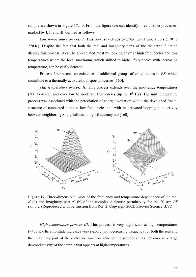
sample are shown in Figure 17a, b. From the figure one can identify three distinct processes,
marked by I, II and III, defined as follows:
Low temperature process I: This process extends over the low temperatures (170 to
270 K). Despite the fact that both the real and imaginary parts of the dielectric function
display this process, it can be appreciated most by looking at ε′′ at high frequencies and low
temperatures where the local maximum, which shifted to higher frequencies with increasing
temperature, can be easily detected.
Process I represents an existence of additional groups of exited states in PS, which
contribute to a thermally activated transport processes [160].
Mid temperature process II: This process extends over the mid-range temperatures
(300 to 400K) and over low to moderate frequencies (up to 105 Hz). The mid temperature
process was associated with the percolation of charge excitation within the developed fractal
structure of connected pores at low frequencies and with an activated hopping conductivity
between neighboring Si crystallites at high-frequency tail [160].
Figure 17. Three-dimensional plots of the frequency and temperature dependence of the real ε' (a) and imaginary part ε'' (b) of the complex dielectric permittivity for the 20 μm PS sample. (Reproduced with permission from Ref. 2. Copyright 2002, Elsevier Science B.V.)
High temperature process III: This process is very significant at high temperatures
(>400 K). Its amplitude increases very rapidly with decreasing frequency for both the real and
the imaginary part of the dielectric function. One of the sources of its behavior is a large
dc-conductivity of the sample that appears at high-temperatures.
46

Similar processes were also observed for the 30 μm thickness samples. The detailed
description of the mechanism of the mid temperature process in the percolation region and
porosity determination in PS will be presented below.
4.3 Ferroelectric crystals
Amongst the perovskite family of ferroelectrics KTN crystals (KTa1-xNbxO3) have
attracted great interest both as model systems and for their optical properties. They were first
systematically studied in 1959 [169] and a complete microscopic description of the
ferroelectric phase transition was given in 2001 [170]. They display both displacive-like and
order disorder-like properties [171-174]. For niobium (Nb) concentrations of x > 0.2 the
ferroelectric phase transition is of the first order and follows the linear rule for ferroelectric
phase transition temperature Tc≈682x [175]. At the ferroelectric phase transition the crystal
structure is transformed from cubic to tetragonal. Further cooling incurs two additional
structural transitions: tetragonal to orthorhombic, and orthorhombic to rhombohedral [175]. It
was recently shown that the interaction of the off-centre Nb ion with the soft mode phonon of
the crystal in fact governs the phase transition [170]. At the phase transition the distortion of
the crystal lattice caused by the off-centre position of the Nb ion leads to the creation of
virtual dipoles in the crystal lattice which are randomly distributed throughout the crystal. The
resultant local fields strongly polarize the lattice leading to long-range cooperativity,
frequently of length scales 1000-10000 Ǻ [176], indicative of the ferroelectric phase. The
addition of transition metal ions to this system leads to further novel properties. Of particular
interest is the addition of small quantities of copper (Cu) ions. Copper, in small
concentrations, approximately 1.5 × 10⁻⁴ molar concentration, is known to greatly enhance the
photorefractive effect in these crystals [177], leading to important electroholographic
applications [178]. Generally Cu ions occupy the potassium site in the lattice and sit off-
centre. This virtual dipole is the source of further relaxations in the crystal.
The dielectric behavior of copper-doped and pure KTN crystals were compared in
wide temperature and frequency ranges in order to study the effect of such small Cu ion
concentrations on the dielectric landscape [179]. The two studied KTN crystals were grown
using the top seeded solution growth method [180]. The Ta/Nb ratio in both crystals was
estimated by Perry’s linear relation [175] linking Tc, to the concentration of Nb,
Tc=682x+33.2, and was found to be approximately 62/38 per mole. The first crystal (crystal
#1) was doped with copper. The doping level was 2% in the flux yielding approximately
47
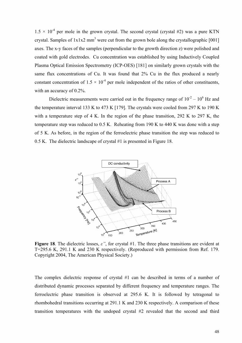
1.5 × 10⁻⁴ per mole in the grown crystal. The second crystal (crystal #2) was a pure KTN
crystal. Samples of 1x1x2 mm3 were cut from the grown bole along the crystallographic [001]
axes. The x-y faces of the samples (perpendicular to the growth direction z) were polished and
coated with gold electrodes. Cu concentration was established by using Inductively Coupled
Plasma Optical Emission Spectrometry (ICP-OES) [181] on similarly grown crystals with the
same flux concentrations of Cu. It was found that 2% Cu in the flux produced a nearly
constant concentration of 1.5 × 10⁻⁴ per mole independent of the ratios of other constituents,
with an accuracy of 0.2%.
Dielectric measurements were carried out in the frequency range of 10-2 – 106 Hz and
the temperature interval 133 K to 473 K [179]. The crystals were cooled from 297 K to 190 K
with a temperature step of 4 K. In the region of the phase transition, 292 K to 297 K, the
temperature step was reduced to 0.5 K. Reheating from 190 K to 440 K was done with a step
of 5 K. As before, in the region of the ferroelectric phase transition the step was reduced to
0.5 K. The dielectric landscape of crystal #1 is presented in Figure 18.
Figure 18. The dielectric losses, ε”, for crystal #1. The three phase transitions are evident at T=295.6 K, 291.1 K and 230 K respectively. (Reproduced with permission from Ref. 179. Copyright 2004, The American Physical Society.)
The complex dielectric response of crystal #1 can be described in terms of a number of
distributed dynamic processes separated by different frequency and temperature ranges. The
ferroelectric phase transition is observed at 295.6 K. It is followed by tetragonal to
rhombohedral transitions occurring at 291.1 K and 230 K respectively. A comparison of these
transition temperatures with the undoped crystal #2 revealed that the second and third
48
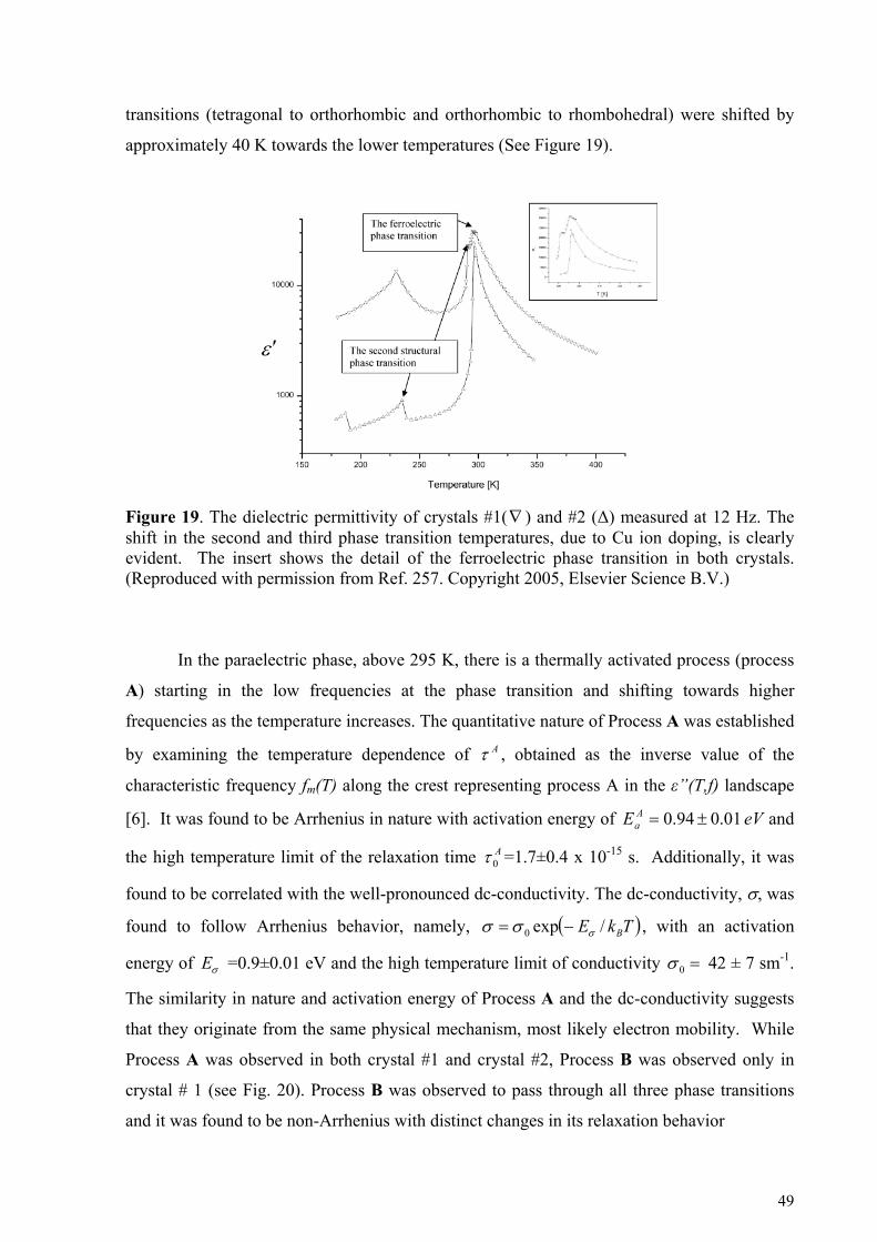
transitions (tetragonal to orthorhombic and orthorhombic to rhombohedral) were shifted by
approximately 40 K towards the lower temperatures (See Figure 19).
Figure 19. The dielectric permittivity of crystals #1(∇ ) and #2 (Δ) measured at 12 Hz. The shift in the second and third phase transition temperatures, due to Cu ion doping, is clearly evident. The insert shows the detail of the ferroelectric phase transition in both crystals. (Reproduced with permission from Ref. 257. Copyright 2005, Elsevier Science B.V.)
In the paraelectric phase, above 295 K, there is a thermally activated process (process
A) starting in the low frequencies at the phase transition and shifting towards higher
frequencies as the temperature increases. The quantitative nature of Process A was established
by examining the temperature dependence of , obtained as the inverse value of the
characteristic frequency fm(T) along the crest representing process A in the ε”(T,f) landscape
[6]. It was found to be Arrhenius in nature with activation energy of and
the high temperature limit of the relaxation time =1.7±0.4 x 10⁻¹⁵ s. Additionally, it was
found to be correlated with the well-pronounced dc-conductivity. The dc-conductivity, σ, was
found to follow Arrhenius behavior, namely,
Aτ
А0τ
eVE Aa 01.094.0 ±=
( )TBkE /exp0 σσσ −= , with an activation
energy of =0.9±0.01 eV and the high temperature limit of conductivity σE =0σ 42 ± 7 sm-1.
The similarity in nature and activation energy of Process A and the dc-conductivity suggests
that they originate from the same physical mechanism, most likely electron mobility. While
Process A was observed in both crystal #1 and crystal #2, Process B was observed only in
crystal # 1 (see Fig. 20). Process B was observed to pass through all three phase transitions
and it was found to be non-Arrhenius with distinct changes in its relaxation behavior
49

Figure 20. A comparison of the dielectric losses measured at T=250 K: ∆ represents crystal #1 (KTN doped with Cu ions) and ○ represents crystal #2 (pure KTN). (Reproduced with permission from Ref. 179. Copyright 2004, The American Physical Society.)
Figure 21. The characteristic relaxation times for Process B. On the figure are marked the three phase transitions and the critical cross-over temperature, T=354 K, between Ahrrenius and VFT behaviours. The circles are the experimental data and the lines are the fitting functions; Ahrrenius, VFT and “Saddle-like” [78,179]. (Reproduced with permission from Ref. 257. Copyright 2005, Elsevier Science B.V.)
delineated by the phase transitions. In the same manner as for Process A relaxation time τB
was extracted from the peak maximum of the dielectric losses, ε”(ω,T), (Figure 21).
In the high temperature range, above 354K, Process B exhibits Arrhenius behavior
with an activation energy =0.37 ± 0.01 eV and = 2.8 ± 0.9 x 10⁻¹² s. Below Tx=354K
Process B obeys a Vogel-Fulcher-Tammann (VFT) relaxation in which τB is given by (2.28)
BaE В
0τ
)VFTT()ln()ln( 0
B
VFTBB
TkE
−+= ττ with TVFT=228K, and EVFT = 0.02 eV. Following the onset of
the ferroelectric phase transition at Tc=295.6 K, τB decreases until it reaches a minimum at
264K, exhibiting a small cusp at the second (tetragonal to orthorhombic) phase transition.
Upon further cooling τB increases until it reaches a maximum at the third (orthorhombic to
rhombohedral) transition at 230K, exhibiting a “saddle” [78] that will be discussed in detail
below.
50
4.4 H-bonding Liquids
The study of slow dynamics in glass forming liquids is currently a significant
challenge in the research field of soft condensed matter science [182-186]. Hydrogen bonding
liquids and their mixtures occupy a special place among complex systems due to existence of
directed H-bonds (in contrast to van der Waals and ionic systems) that can be rearranged
relatively easily (in contrast to covalent bonds). Although an enormous amount of literature
exists which relates to the investigation of hydrogen-bonding systems (See for example
[3,183,185]) there is still a lack of clear understanding of their dynamics, structure and glass
transitions. Among them, glycerol (C3H8O3) [17,74,187-189] and its mixtures with water
[190] is widely used as excellent model to study their cooperative dynamics.
Usually, glycerol exists only in liquid, supercooled, or glassy states. However, after
special treatment pure dehydrated glycerol can be crystallized [191,192]. Uncrystallized
glycerol is a common system used for studying glass-forming dynamics [3,184,187-189,193-
195] while crystallized glycerol, until now, has not been investigated.
Under normal conditions glycerol does not undergo crystallization but rather during
cooling it becomes a supercooled liquid which can be vitrified [184,187,196,197] at Tg=190
K. In contrast, anhydrous glycerol, cooled down below the glass transition point Tg and then
slowly heated up, can be crystallized. However, crystallization of glycerol is a very unusual
and unstable process, which depends on the temperature history and impurities of the sample.
The main features of glycerol crystallization were studied [186] by comparing the glass-
forming dynamics of anhydrous glycerol (Sample A) with those of glycerol that was not
specially treated to prevent water absorption (Sample B). To reach crystallization, sample A
was cooled from room temperature to 133 K. Then measurements of the complex dielectric
permittivity ε*(ω) were performed by a Novocontrol Alpha Analyzer in the frequency interval
0.01 Hz - 3 MHz and the temperature range 133 K - 325 K (See Figure 22). Thus, overall
experimental time was 30 h and average heating rate was about 0.1K min-1. Considerable
changes in ε*(ω) behavior in the measured frequency range are observed in the temperature
interval from 263 K to 293 K. The transition at 293 K is known as the glycerol melting point
[198]. Thus, the transition near 263 K is thought to be attributed to the glycerol
crystallization.
Note that the relaxation process (I) of the supercooled glycerol in this temperature
interval disappears and the relaxation process (II), with a reduced strength, appears in the low
frequency region.
51

Figure 22. A three-dimensional plot representing the real part of ε′(ω) for sample A. The arrows mark the crystallization temperature (Tx =263 K), the melting point (Tm=293 K), and the principal relaxation process, before (I) and after (II) the crystallization. (Reproduced with permission from Ref. 186. Copyright 2003, The American Physical Society.)
Figure 23. Sample A before (unfilled boxes) and after (filled boxes) the crystallization compared with sample B (triangles), and literature data [195] (circles). In the supercooled phase all samples obey a VFT law (full lines), while the relaxation process in sample A above 263 K obeys an Arrhenius law (dash-dotted line). (Reproduced with permission from Ref. 186. Copyright 2003, The American Physical Society.)
The data presented in Fig.23 were analyzed as a set of isothermal spectra in the
framework of (2.21)
βατωεεεε
))(1()(*
if s
+−
+= ∞∞
It is remarkable that in the liquid and supercooled phase glycerol exhibits unsymmetrical
relaxation peak broadening (α ≈ 1, β ≈ 0.6) whereas in the case of process (II) the broadening
is a rather symmetric one (0.6 ≤ α ≤ 0.7, β =1). The Arrhenius plot in Figure 23 shows that
relaxation dynamics in the supercooled glycerol phase before crystallization (I) obey the VFT
relationship while after crystallization (II) follow Arrhenius law. Note, that in the considered
frequency and temperature landscape, another low frequency process related to the
crystallization is observed. Unfortunately, it was not resolved properly in the mentioned study
[186].
The VFT behavior of supercooled glycerol is well known from studies of liquid and
supercooled glycerol [3,186-190] while the Arrhenius dependence of dielectric relaxation
52

time is more relevant for crystals. For example, the temperature dependence of dielectric
relaxation time of ice I also obeyes Arrhenius law with the activation energy about
60 kJ⋅mol-1[198,199].
Therefore, the observed process (I) could be related to cooperative dynamics of
glycerol in the supercooled phase while process (II) is most likely related to the crystalline
phase of glycerol and is the result, similar to water, of the mobility of defects in the crystalline
lattice [200]. The temperature dependence of the relaxation time for the dehydrated glycerol is
compared in Figure 23 with those for the usual behavior of glycerol, which has absorbed
some water from the atmosphere.
In Figure 23, we compared temperature dependencies of fitted relaxation time for
samples A and B and data recently published by Lunkenheimer and Loidl [195]. The fitting
yields that the process (I) in the supercooled phase for sample A, the relaxation in sample B,
and literature data [195], all obey the VFT law ( ){ }vvv TTDT −= /expmax ττ where Tv is the
Vogel-Fulcher temperature, τv is the pre-exponential factor, and D is the fragility parameter.
From the data presented in Figure 23 one can see that values of the VFT temperature Tv and
fragility D are very close for all the samples where D = 22±2 and Tv = 122±2 K, while the
preexponential factors τv are remarkably different. For the anhydrous sample A,
τv = 3.93×10⁻¹⁶ s, for sample B, τv = 2.3×10⁻¹⁶ s, while for the literature data [195]
τv = 1.73×10⁻¹⁶ s. Taking into account the fact that sample A was specially protected from
water absorption, it is strongly suspected that this significant difference in τv is caused by the
water absorbed from the atmosphere. This observation signifies that even very small water
content can result in significantly different dynamics in the supercooled phase for the
anhydrous glycerol and for the glycerol samples usually studied [186].
As mentioned above, the frequency dependence of complex dielectric permittivity
( ) of the main relaxation process of glycerol [17,186] can be described by the Cole-
Davidson (CD) empirical function (See (2.21) with α =1,
*ε
10 ≤< CDβ ). In that case τCD is the
relaxation time which has non-Arrhenius type temperature dependence for glycerol (See
Figure 23). Another well known possibility is to fit the BDS spectra of glycerol in time
domain using the KWW relaxation function (2.23) φ(t) (See Figure 24).
53

Figure 24. The imaginary parts of the dielectric spectrum for anhydrous glycerol in the supercooled state at 196 K [186]. The dotted and dashed line show descriptions of the main relaxation process by CD [Eq. (21)] with CDτ = 2.61 s, Δε = 63.9 and CDβ = 0.51) and KWW [Eq. (23)] with Kτ = 1.23 s, Δε = 62.0 and Kβ = 0.69) functions, respectively. (The half-width of the loss curve were fixed for both CD and KWW functions.) (Reproduced with permission from Ref. 208. Copyright 2005, American Chemical Society.)
The CD function predicts the dielectric loss (ε”) of glycerol to follow the power law
ε”~ towards the high frequencies ( ), where fmax is the frequency corresponding
to the dielectric loss peak. However, the high frequency experimental data in Figure 24
demonstrate a significant deviation from the expected asymptotic behavior both for CD and
KWW functions. The finding of ε” values larger than predicted by the spectral function of the
main relaxation are known as the excess wing (EW). Although there is no unique
interpretation of the EW, it is known that this phenomenon is a property of many glass-
forming systems [195,201-203]. Note that deviations from a power law slope for ε” were also
observed for pure water [204-206]. These features were treated as an additional Debye type
relaxation process without any relation to glass-forming properties. However, with given
glass forming properties of water, they can be discussed as the EW feature as well. There is
some discussion [201] that the EW is most probably a Johari-Goldstein (JG) [207] mode.
However, there are still open questions because analysis of pressure and temperature effects
leads to the conclusion that EW and JG modes “cannot be treated on the same footing” [202].
The non-Arrhenius temperature dependence of the EW found recently [203] is in
contradiction to the original idea of Johari and Goldstein who argued, “the Arrhenius plots in
the secondary relaxation region are linear” [207]. Thus the relaxation mechanism of the EW
is still unclear, and it would be helpful to study how the water concentration in glycerol
CDf βmaxff >>
54

influences the relaxation dynamics of the mixture, since the EW could be related to the feature
of H-bond networks of glycerol that are being affected by the presence of water.
The typical results of recent BDS studies of glycerol-water mixtures of 75 mol% of
glycerol at different temperatures are presented in Figure 25 [208]. Figure 26 shows that the
temperature dependencies of the main relaxation process in the terms of ( )maxmax 2/1 fπτ = for
concentrations from 100 to 40 mol% of glycerol were well described by the VFT law.
Figure 25. The imaginary parts of the dielectric spectra for a glycerol–water mixture (75 mol%) at various temperatures from 197 to 290 K with an interval of 3 K. (Reproduced with permission from Ref. 208. Copyright 2005, American Chemical Society.)
Figure 26. Temperature dependence of ( )maxmax 2/1 fπτ = for a glycerol sample and its
mixtures with water. The solid curves show the description by the VFT model, where values of the Vogel–Fulcher temperature (Tv) are shown with the legend. The preexponential factor (τv) is almost independent with concentration:ln (τv) = –35.9 for 100 mol% of glycerol, –36.1 for 95 to 65%, –36.2 for 60%, –36.3 for 60 to 45% and –36.4 for 40 mol% of glycerol–water mixtures. D = 22.7 for all concentrations presented here. (Reproduced with permission from Ref. 208. Copyright 2005, American Chemical Society.)
It is worth noting that value of D was the same for all concentrations presented in Figure 26
and values of τv were also almost the same in this concentration range.
Let us start the examination of the dynamics of glycerol-water mixtures with an
inspection of the main dielectric loss peak ε”max = ε”(fmax) with fmax as the characteristic
frequency that was observed in the considered experimental ranges for glycerol and its
mixtures with water. Figure 27 presents a so-called “master plot” that presents the normalized
plots of ε”(f) / ε”max versus the dimensionless variable f / fmax. Namely, each data point in the
dielectric spectrum was normalized by only one point such as the loss peak. It is remarkable
55
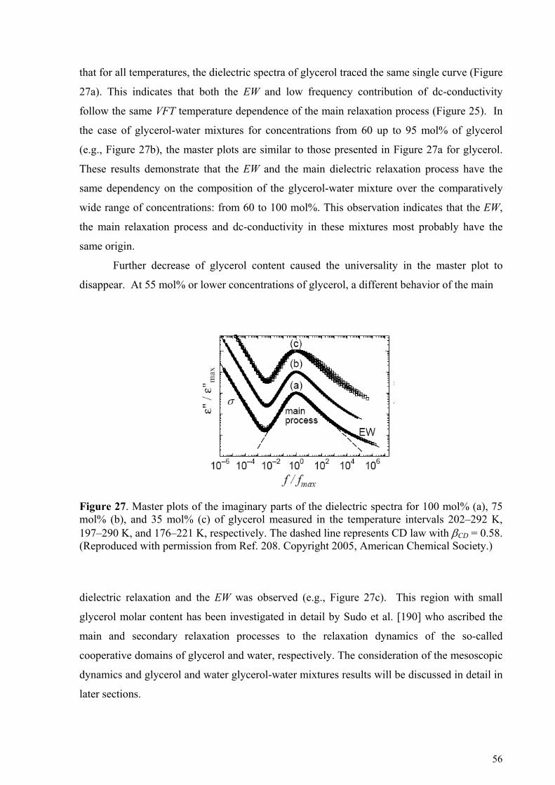
that for all temperatures, the dielectric spectra of glycerol traced the same single curve (Figure
27a). This indicates that both the EW and low frequency contribution of dc-conductivity
follow the same VFT temperature dependence of the main relaxation process (Figure 25). In
the case of glycerol-water mixtures for concentrations from 60 up to 95 mol% of glycerol
(e.g., Figure 27b), the master plots are similar to those presented in Figure 27a for glycerol.
These results demonstrate that the EW and the main dielectric relaxation process have the
same dependency on the composition of the glycerol-water mixture over the comparatively
wide range of concentrations: from 60 to 100 mol%. This observation indicates that the EW,
the main relaxation process and dc-conductivity in these mixtures most probably have the
same origin.
Further decrease of glycerol content caused the universality in the master plot to
disappear. At 55 mol% or lower concentrations of glycerol, a different behavior of the main
Figure 27. Master plots of the imaginary parts of the dielectric spectra for 100 mol% (a), 75 mol% (b), and 35 mol% (c) of glycerol measured in the temperature intervals 202–292 K, 197–290 K, and 176–221 K, respectively. The dashed line represents CD law with βCD = 0.58. (Reproduced with permission from Ref. 208. Copyright 2005, American Chemical Society.)
dielectric relaxation and the EW was observed (e.g., Figure 27c). This region with small
glycerol molar content has been investigated in detail by Sudo et al. [190] who ascribed the
main and secondary relaxation processes to the relaxation dynamics of the so-called
cooperative domains of glycerol and water, respectively. The consideration of the mesoscopic
dynamics and glycerol and water glycerol-water mixtures results will be discussed in detail in
later sections.
56

5 Cooperative dynamic and scaling phenomena in
disordered systems Following the general plan of our tutorial, we will discuss here a universal view of
scaling which is widely employed in modern dielectric spectroscopy. We will show how this
concept can be applied to the description of disordered materials and how these ideas can be
useful in the determination of the topological parameters of these systems.
5.1 Static percolation in porous materials, Fractal concept and
porosity determination In this section, we will consider in more detail the non-Debye dielectric response
associated with percolation in porous disordered materials: silica glasses and porous silicon
where the pores form topologically connected pore channels. The movement of charge
carriers along the inner pore surface results in a transfer of the electric excitation within the
channels along random paths [154]. Note that in the general case such transfers through the
porous medium can occur even in the case of closed pores, which are topologically not
connected one to another. However, the distance between the neighboring pores filled with
the dielectric or conductive material should be small enough in order to provide “physical”
pore coupling via the electric interaction.
It was shown that disordered porous media can been adequately described by the
fractal concept, where the self–similar fractal geometry of the porous matrix and the
corresponding paths of electric excitation govern the scaling properties of the DCF Ψ(t) (See
Relationship (2.22)) [154,209]. In this regard we will use the theory of electronic energy
transfer dynamics developed by Klafter, Blumen and Shlesinger [210,211], where a transfer
of the excitation of a donor molecule to an acceptor molecule in various condensed media
through many parallel channels was considered.
A detailed description of the relaxation mechanism associated with an excitation
transfer based on a recursive (regular) fractal model was introduced earlier [47], where it was
applied for the cooperative relaxation of ionic microemulsions at percolation.
According to this model, an elementary act of the excitation transfer along the length
Lj is described by the microscopic relaxation function g(z/zj), where Lj is the "effective"
length of a channel of the relaxation in the j-th stage of self-similarity. In this function, zj is a
dimensional variable characterizing the j-th stage of the self-similarity of the fractal system
57

considered, z is the dimensionless time, z = t/τ, where the parameter τ is the minimal
relaxation time needed for an excitation to hop from one excitation center to its nearest
neighbor.
The following assumption is invoked: zj = aLj, where a is a coefficient of
proportionality. For each stage of the self-similarity j, the time of relaxation τj = τ zj is
proportional to the length Lj. From fractal geometry [212,213] Lj can be expressed as
j
j lkL = , (5.1)
where l is the minimal scale and k is a scaling factor (k > 1). We assume that the total number
of activation centers located along the segment Lj also obeys the scaling law
j
0j p n n = , (5.2)
where p is the scaling factor (p > 1), and n0 is the number of the nearest neighbors near the
selected center (i.e., j = 0).
The macroscopic correlation function can be expressed as a product of the relaxation
functions g(z/zj) for all stages of self-similarity of the fractal system considered [47,154]
( ) ( )[ ] ( )[ ]Ψ z g z z g Zjj
N nj
j
N n pjj
= == =
∏ ∏/0 0
0
ξ,
(5.3)
where Z = t/alτ; ξ = 1/k and Nk
L lN=1
lnln( / ) . Here LN is the finite geometrical size of the
fractal cluster and N refers to the last stage of self-similarity.
The estimations of the product (5.3) for various values of ξ < 1 and p > 1 are given in
Ref.47. The results of the calculations may be written in the form of a modified Kohlrausch-
Williams-Wats (KWW) stretched-exponential relaxation law:
( ) ( ) [ ]ZBZZ )()(exp0/ νν ν +Γ−=ΨΨ , (5.4)
where the parameters Γ(ν) and B(ν) are given by
58

( ) ( )( )Γ ν
ξν= −
∞
∫n
yg yg y
dy0
01ln( / )
'
,
(5.5)
n aln
0 1
( / )( )ν . .(5.6)
1 11
ξε ν
−−B(ν) =
Here
( )ξν /1ln/ln p= (5.7)
with 0 < ν < 1, and for ε = ξN << 1. We note that the parameter Γ depends on the relaxation
function g and affects the macroscopic relaxation time τM = τ alΓ -1/ν, and the term B(ν)Z in
the exponent corrects the KWW function at large times.
The temporal boundaries of the applicability of (5.4) are determined by the expression:
A ng ln
tal
lnn a a
1 0
0 2 12 2
1 212 1 1
2 1 22
(1
( / )( )( / )( )
( )
/
−+
<< <<−
−⎛⎝⎜
⎞⎠⎟−ξ ν τ
ξ νε ν
. (5.8)
The parameters g , A1, a1, and a2 in (5.4)-(5.8) are related to the asymptotic properties of the
elementary relaxation function g(y):
g y a y a y( ) ...= − + +1 1 22 , for y<<1 , (5.9)
g y g A y A y( ) / / ...= + + +1 22 , for y >> 1 . (5.10)
The relationship between the exponentν, (
ν =ln pln k
) , and the fractal dimension Dp of the
paths of excitation transfer may be derived from the proportionality and scaling relations by
using an assumption that the fractal is isotropic and has spherical symmetry. The number of
pores that are located along a segment of length Lj on the j-th step of the self-similarity
is nj ~ pj. The total number of pores in the cluster is S ~ njd ~ (pj)d, where d is the Euclidean
dimension, (d = 3). The similarity index, η, which determines by how much the linear size of
the fractal is enlarged at step j, is η ~ Lj ~ k j. In this case, we obtain the simple relationship
between ν and the fractal dimension Dp as
59

νη 3ln/ln3ln/ln === kjpjSDp . (5.11)
Further we will focus our attention only on the time dependant behavior of the dipole
correlation function Ψ(t) defined by (5.4), that is given by
Ψ ( ) ( ) exp[ ( / ) ]t C t t≈ − τ ν, (5.12)
where C(t) is the slow growing function of time. By taking into account (5.11) and ignoring
the slow variation with time of C(t), we obtain the asymptotic stretched-exponential term
Ψ ( ) ~ exp[ ( / ) ]/t t Dp− τ 3 (5.13)
that can be further fitted to the experimental correlation functions in order to determine the
value of the fractal dimension of the paths of excitation transfer within the porous medium. If
the fractal dimension of these paths coincides with the fractal dimension of the pore space,
then it can be used in the asymptotic equations derived below for the porosity determination.
5.1.1 Porous glasses
The dielectric relaxation at percolation was analyzed in time domain since the theoretical
relaxation model described above is formulated for the dipole correlation function Ψ(t). For
this purpose the complex dielectric permittivity data were expressed in terms of the DCF
using (2.14) and (2.25). Figure 28 shows typical examples of the DCF, obtained from the
frequency dependence of the complex permittivity at the percolation temperature,
corresponding to several porous glasses studied recently [153-156].
As mentioned earlier the typical three-dimensional plots of ε′ and ε″ versus frequency and
temperature (see Figure 14) indicates the superposition of two processes (percolation and
saddle-like) in the vicinity of the percolation. Therefore, in order to separate the long-time
percolation process, the DCF was fitted as a sum of two functions.
The KWW function (5.13) was used for fitting the percolation process and the product
(2.25) of the power law and the stretched exponential function (as a more common
representation of relaxation in time domain) was applied for the fitting of the additional short-
time process.
60

10-6 10-5 10-4 10-3 10-2 10-1
0.0
0.2
0.4
0.6
0.8
1.0
Ψ (t
)
t , [s]
Figure 28. Semilog plot of the dipole correlation ψ (t) of all the samples studied at the temperature corresponding to percolation (□ sample A; ○ sample B; ∆ sample C; ∇ sample D; ◊ sample E; × sample F; sample G). The solid lines are the fitting curves of the sum of the KWW and the product of KWW and the power-law relaxation function. (Reproduced with permission from Ref. 2. Copyright 2002, Elsevier Science B.V.)
∗
The values obtained for Dp of different porous glasses are presented in the Table 1. The
glasses studied differed in their preparation method, which affects the size of the pores,
porosity and availability of second silica and ultra-porosity [153-156].
One can see that the fractal dimension of the excitation paths in sample A is close to unity.
Topologically, this value of Dp corresponds to the propagation of the excitation along a linear
path that may correspond to the presence of second silica within the pores of the sample A.
Indeed, the silica gel creates a subsidiary tiny scale matrix with an enlarged number of
hydration centers within the pores. Since these centers are distributed in the pore volume, the
excitation transmits through the volume and is not related to the hydration centers located on
the pore surface of the connective pores. Due to the large number of hydration centers, and
the short distance between the neighboring centers, the path can be approximated by a line
with a fractal dimension close to unity (See Figure 29a).
61
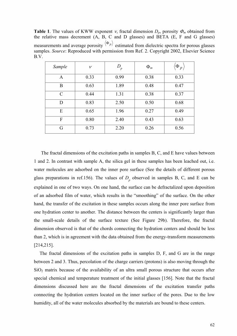
Table 1. The values of KWW exponent ν, fractal dimension Dp, porosity Φm obtained from the relative mass decrement (A, B, C and D glasses) and BETA (E, F and G glasses)
measurements and average porosity pΦ estimated from dielectric spectra for porous glasses samples. Source: Reproduced with permission from Ref. 2. Copyright 2002, Elsevier Science B.V.
Sample ν Dp Φm pΦ
A 0.33 0.99 0.38 0.33
B 0.63 1.89 0.48 0.47
C 0.44 1.31 0.38 0.37
D 0.83 2.50 0.50 0.68
E 0.65 1.96 0.27 0.49
F 0.80 2.40 0.43 0.63
G 0.73 2.20 0.26 0.56
The fractal dimensions of the excitation paths in samples B, C, and E have values between
1 and 2. In contrast with sample A, the silica gel in these samples has been leached out, i.e.
water molecules are adsorbed on the inner pore surface (See the details of different porous
glass preparations in ref.156). The values of Dp observed in samples B, C, and E can be
explained in one of two ways. On one hand, the surface can be defractalized upon deposition
of an adsorbed film of water, which results in the “smoothing” of the surface. On the other
hand, the transfer of the excitation in these samples occurs along the inner pore surface from
one hydration center to another. The distance between the centers is significantly larger than
the small-scale details of the surface texture (See Figure 29b). Therefore, the fractal
dimension observed is that of the chords connecting the hydration centers and should be less
than 2, which is in agreement with the data obtained from the energy-transform measurements
[214,215].
The fractal dimensions of the excitation paths in samples D, F, and G are in the range
between 2 and 3. Thus, percolation of the charge carriers (protons) is also moving through the
SiO2 matrix because of the availability of an ultra small porous structure that occurs after
special chemical and temperature treatment of the initial glasses [156]. Note that the fractal
dimensions discussed here are the fractal dimensions of the excitation transfer paths
connecting the hydration centers located on the inner surface of the pores. Due to the low
humidity, all of the water molecules absorbed by the materials are bound to these centers.
62

(a)
(b)
Figure 29. The schematic presentation of the percolation pass in porous glasses; (a) The glass whose porous are filled with second silica; (b) The porous glasses where the silica gel is leached out.
The paths of the excitation transfer span along the fractal pore surface and “depict” the
backbone of clusters formed by the pores on a scale that is larger than the characteristic
distance between the hydration centers on the pore surface. Thus, a fractal dimension of the
paths Dp approximates the real surface fractal dimension in the considered scale interval. For
random porous structures, Dp can be also associated with the fractal dimension Dr of the
porous space: Dp ≅ Dr. Therefore, the fractal dimension Dp can be used for porosity
calculations in the framework of the fractal models of the porosity.
The porosity Φp of a two-phase solid-pore system can be defined as the ratio of the volume
of the empty space, Vp, to the whole volume, V, of a sample [166]:
VVp
p =Φ.
(5.14)
Disordered porous media have been adequately described by the fractal concept
[154,216]. It was shown that if the pore space is determined by its fractal structure, the
regular fractal model could be applied [154]. This implies that for the volume element of
linear size Λ, the volume of the pore space is given in units of the characteristic pore size λ by
, where Dr is the regular fractal dimension of the porous space, Λ coincides
with the upper limit and λ with the lower limit of the self-similarity. The constant Gg is a
( ) rDgp GV λ/Λ=
63

geometric factor. Similarly, the volume of the whole sample is scaled as V = Gg (Λ/λ)d, where
d is the Euclidean dimension (d=3). Hence, the formula for the macroscopic porosity in terms
of the regular fractal model can be derived from (5.14), and is given by:
rDd
p
−⎟⎠⎞
⎜⎝⎛
Λ=Φ
λ .
(5.15)
In general, in order to include more types of porous media the random fractal model can be
considered [2,154,216]. Randomness can be introduced in the fractal model of a porous
medium by the assumption that the ratio of the scaling parameters ξ=λ/Λ is random in the
interval [ξ0, 1], but the fractal dimension D in this interval is a determined constant. Hence,
after statistical averaging (5.15) reads as
( ) ( ) ξξξξ
dwDrpp ∫ Φ=Φ1
0
, , (5.16)
where ξ0 is the minimal value of the scaling parameter ξ and w(ξ)dξ measures the probability
to find some scaling parameter in the range from ξ to ξ+dξ.
For a percolating medium the generalized exponential pore-size distribution function of the
scale for porous medium can be written as
)exp(~)( ww bwaw ξξξ α − . (5.17)
This function accounts for the mesoscale region and comprises most of the listed distribution
functions [154]. It includes three empirical parameters, αw, βw, and aw. After ascertaining the
relationships between these parameters and the properties of anomalous self-diffusion, fractal
morphology, and polydispersity of the finite pore-size, physical significance can be assigned
to these parameters in the framework of the percolation models [152].
On the length scale, which is larger than the pore sizes, the morphology of the glass porous
space can be modeled as a random-packed assembly of clusters formed by pores connected to
each other [203,217]. In order to find the macroscopic porosity in such systems we must
assume that the pore structure has a fractal character in a rather narrow scale range. Hence, in
the interval [ξ0, 1] the uniform distribution function, w(ξ) = w0, can be chosen as an
approximation of the function derived by (5.16). The value of w0 is determined from the
64

normalization condition , and reads as 1)(10
=∫ξ ξξ dw0
0 11ξ−
=w . In this approximation, by
substituting this uniform distribution function into integral (5.16) and integrating it, we obtain
the relationship for the average porosity as
0
101
11
1ξ
ξ−
−⋅
−+=Φ
−+ rDd
rp Dd .
(5.18)
Taking into account that ξ0 << 1, and 1+d-Dγ >0 (since topologically Dγ < 3, and d = 3),
we obtain a simple approximate relationship between the average porosity of a glass and the
fractal dimension of the pore space, which reads
rp D4
1 −
≈Φ .
(5.19)
Note that in our approximation, due to the randomized character of the fractal medium the
average porosity of the disordered porous glasses determined by (5.19) depends only on the
fractal dimension Dr and does not exhibit any scaling behavior. In general, the magnitude of
the fractal dimension may also depend on the length scale of a measurement extending from λ
to over Λ, where the minimal scale λ and the maximal scale Λ are determined by the
measurement technique.
The results of the porosity calculation for different porous glasses using (5.19) together
with the fractal dimension determined from dielectric measurements are shown in the last
column of Table 1. These values can be compared with the porosity Φm determined from the
relative mass decrement (A, B, C and D glasses) and BETA (E, F and G glasses)
measurements shown in the same Table 1. Note that the values obtained from dielectric
spectroscopy coincide with the porosity data obtained from the relative mass decrement
method only for samples A, B and C. The porosity values for the other samples obtained
through the dielectric measurements are significantly larger. This correlates with the
availability of ultra small porous structures with penetrability for the smallest charge carriers
(such as protons) [156]. Thus, in the case of a net of super small open pores, the dielectric
response is more sensitive and accurate in the determination of real porosity than any other
conventional method.
65

5.1.2 Porous silicon
The detailed analysis of mid-temperature relaxation processes observed in porous silicon
was provided recently by using a superposition of two Jonscher terms of the form,
[160]. The results of our fitting were in good agreement with those
of Ben-Chorin et al. [163] that were discussed in terms of the transport of charged carriers at
the different scales. The high frequency Jonscher exponent was associated with the typical
size of the Si nano-crystallites, while the low-frequency (LF) exponent was assigned to the
transport of charged carriers across a disordered fractal structure of porous silicon
[160,161,218,219]. At the same time the mid temperature process II demonstrates several
specific features that are similar to those observed in other porous systems discussed in the
previous section [153-156]. The amplitude of this process essentially decreases when the
frequency increases (Figure 17a). Furthermore, the maximum of the dielectric permittivity
versus temperature has almost no temperature dependence. Finally, the low-frequency ac-
conductivity increases with the increase in temperature and has an S-shaped dependency
(Figure 30), which is typical for percolation processes [143,154,161]. Thus, we will analyze
12
11 21 )()( −− + uu iBiB ωω
300 320 340 360 380 40010-11
10-10
10-9
10-8
C
ondu
ctiv
ity [
(Ω×c
m)-1
]
Tem perature [ K ]
-6 -5 -4 -3 -2 -1 00,0
0,2
0,4
0,6
0,8
1,0
Ψ (t
)
Log t [s]
Figure 30. Temperature dependence of the low-frequency conductivity of the 20-μm sample (●), and the 30-μm sample (▲). (Reproduced with permission from Ref. 2. Copyright 2002, Elsevier Science B.V.)
Figure 31. Semilog plot of the macroscopic correlation function of the 20-μm sample (●) and the 30-μm sample (▲) at the temperature corresponding to percolation. The solid lines correspond to the fitting of the experimental data by the KWW relaxation function. (Reproduced with permission from Ref. 2. Copyright 2002, Elsevier Science B.V.)
66
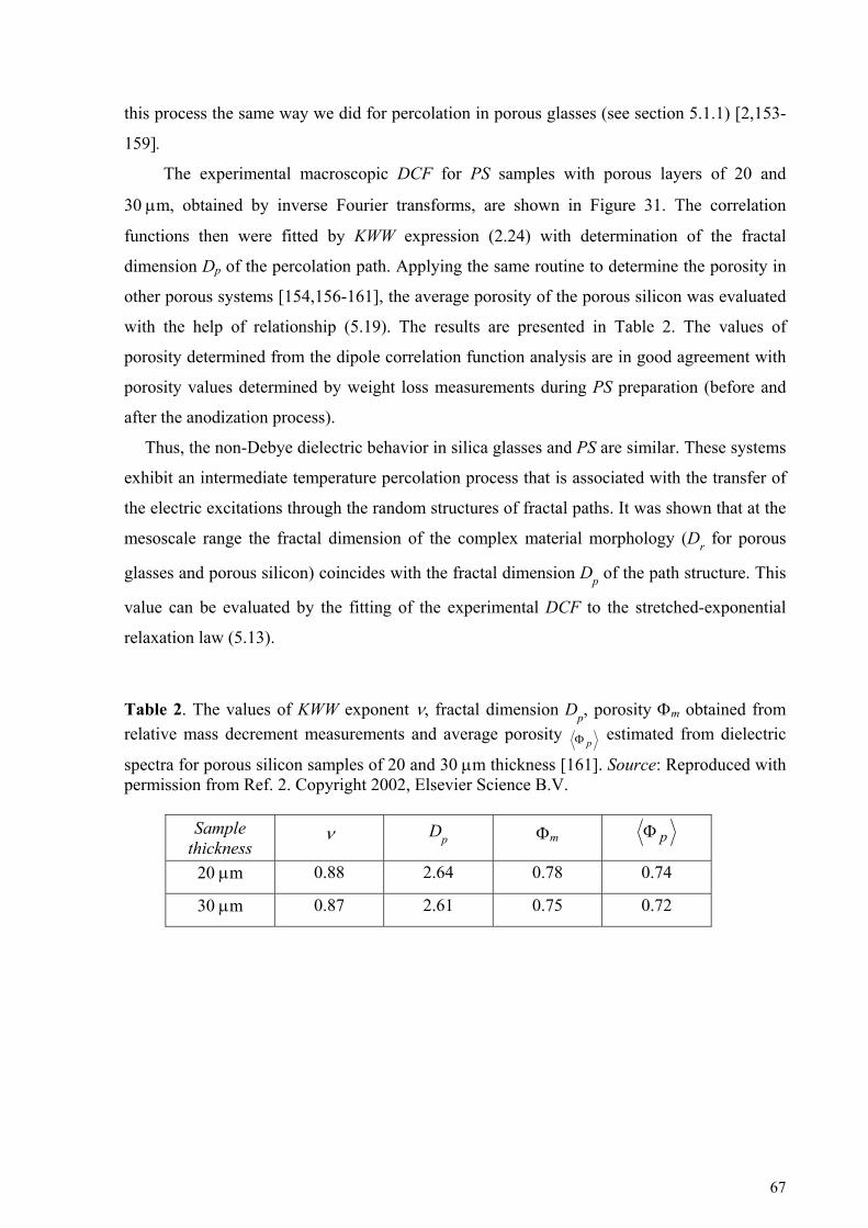
this process the same way we did for percolation in porous glasses (see section 5.1.1) [2,153-
159].
The experimental macroscopic DCF for PS samples with porous layers of 20 and
30 μm, obtained by inverse Fourier transforms, are shown in Figure 31. The correlation
functions then were fitted by KWW expression (2.24) with determination of the fractal
dimension Dp of the percolation path. Applying the same routine to determine the porosity in
other porous systems [154,156-161], the average porosity of the porous silicon was evaluated
with the help of relationship (5.19). The results are presented in Table 2. The values of
porosity determined from the dipole correlation function analysis are in good agreement with
porosity values determined by weight loss measurements during PS preparation (before and
after the anodization process).
Thus, the non-Debye dielectric behavior in silica glasses and PS are similar. These systems
exhibit an intermediate temperature percolation process that is associated with the transfer of
the electric excitations through the random structures of fractal paths. It was shown that at the
mesoscale range the fractal dimension of the complex material morphology (Dr for porous
glasses and porous silicon) coincides with the fractal dimension Dp of the path structure. This
value can be evaluated by the fitting of the experimental DCF to the stretched-exponential
relaxation law (5.13).
Table 2. The values of KWW exponent ν, fractal dimension Dp, porosity Φm obtained from relative mass decrement measurements and average porosity
pΦ estimated from dielectric
spectra for porous silicon samples of 20 and 30 μm thickness [161]. Source: Reproduced with permission from Ref. 2. Copyright 2002, Elsevier Science B.V.
Sample thickness
ν Dp Φm pΦ
20 μm 0.88 2.64 0.78 0.74
30 μm 0.87 2.61 0.75 0.72
67

5.2 Dynamic percolation in ionic microemulsions
5.2.1 Dipole correlation function for the percolation process
A description of the percolation phenomenon in ionic microemulsions in terms of the
macroscopic DCF will be carried out based on the static lattice site percolation (SLSP) model
[152]. In this model the statistical ensemble of various size clusters is described by the
distribution function
( ) ⎟⎟⎠
⎞⎜⎜⎝
⎛−⋅= Ω−
mwm s
ssCssw exp,.
(5.20)
Here Cw is the normalization constant, Ω is a scaling exponent of the probability density "per
lattice site" that the site, chosen randomly, belongs to the s-cluster (a cluster that consist of s
lattice sites). The value of sm is the cut-off cluster size that corresponds to the maximal cluster
size. We note that the exponent Ω is related to the exponent τ of the commonly used cluster
size distribution by the relationship Ω τ−= 1 [152,213,220]. Note that clusters having sizes
in the interval of 1< s < sm are referred to as mesoscopic clusters. The scaling properties of the
mesoscopic dipole correlation functions related to the s-cluster of the geometrical substrate
can be utilized for establishing a link between the static lattice geometrical percolation model
and the relaxation functions.
We assumed that the mesoscopic relaxation function has a simple exponential form:
[ ] [ ])(exp)(, szzszzg ss −= . (5.21)
Here the dimensionless time 1ttz = is normalized by the characteristic relaxation time t1, the
time required for a charge carrier to move the distance equal to the size of one droplet, which
is associated with the size of the one cell in the lattice of the static site–percolation model.
Similarly, we introduce the dimensionless time 1ttz ss = where ts is the effective correlation
time of the s-cluster, and the dimensionless time 1ttz mm = . The maximal correlation time tm
is the effective correlation time corresponding to the maximal cluster sm. In terms of the
random walker problem, it is the time required for a charge carrier to visit all the droplets of a
maximal cluster sm. Thus, the macroscopic DCF may be obtained by the averaging procedure
68

( )[ ] ( )[ ] ( )dssswszzgszz msmm , ,,1∫∞
=Ψ.
(5.22)
In the framework of the SLSP model the relationship between the fractal dimension Ds of the
maximal percolating cluster, the value of its size sm and the linear lattice size L is determined
by the asymptotic scaling law [152,213,220].
Dmsc
lL 1
1= , (sm →∞ , D>0), (5.23)
where l is the linear size of the lattice cell and c1 is a coefficient of proportionality.
Let us assume that on the temporal scale at percolation there is a scaling relationship
between the characteristic relaxation time 1/ ttz mm = and the value of its size sm (similar to
space scaling relationship (5.23), i.e.
( )0 , ,2 >α∞→= αmmm sscz , (5.24)
where c2 is a constant. Additionally, we assume that the self-similarity on the temporal scales
is maintained also for clusters of size s<sm , i.e.
( ) αscszs 2= , (s<sm) (5.25)
Taking into account relationships (5.24) and (5.25), over the long time interval 1>>z the
integration of (5.22) may be performed asymptotically by the saddle-point method [135]. The
main term of the asymptotic expansion can be obtained as the product of the power and
stretched exponential universal relaxation laws [38]:
( ) ( )
⎥⎥⎦
⎤
⎢⎢⎣
⎡⎟⎟⎠
⎞⎜⎜⎝
⎛−=
⎥⎥⎥
⎦
⎤
⎢⎢⎢
⎣
⎡
⎟⎟⎠
⎞⎜⎜⎝
⎛⋅−≅Ψ
ν
μ−α+
α+Ω−
mzzzA
czQzCz expexp
11
2
1221
, (5.26)
where , KCC w= ( ) )1(2)1(2
)1(2
α+Ω−+α
αα+α
π= msK , and
( ) ( )α+−Ω=μ 1212 , ( )α+=ν 11 , ( ) ( )αα αα
+⋅= +− 11msQ . (5.27)
69
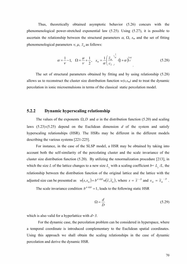
Thus, theoretically obtained asymptotic behavior (5.26) concurs with the
phenomenological power-stretched exponential law (5.25). Using (5.27), it is possible to
ascertain the relationship between the structural parameters α, Ω, sm and the set of fitting
phenomenological parameters ν, μ, mz as follows:
( ) ααα
ααν
μν
α+
+⋅⎟⎟⎠
⎞⎜⎜⎝
⎛=+=Ω−=
11
2
11,21,11
czs m
m
. (5.28)
The set of structural parameters obtained by fitting and by using relationship (5.28)
allows us to reconstruct the cluster size distribution function w(s,sm) and to treat the dynamic
percolation in ionic microemulsions in terms of the classical static percolation model.
5.2.2 Dynamic hyperscaling relationship
The values of the exponents D,Ω and α in the distribution function (5.20) and scaling
laws (5.23)-(5.25) depend on the Euclidean dimension d of the system and satisfy
hyperscaling relationships (HSR). The HSRs may be different in the different models
describing the various systems [221-225].
For instance, in the case of the SLSP model, a HSR may be obtained by taking into
account both the self-similarity of the percolating cluster and the scale invariance of the
cluster size distribution function (5.20). By utilizing the renormalization procedure [213], in
which the size L of the lattice changes to a new size Lc with a scaling coefficient b= Lc /L, the
relationship between the distribution function of the original lattice and the lattice with the
adjusted size can be presented as ( ) ( )mDd
m sswbssw ~,~, Ω−= , where Dss −= ~ and Dmm ss −= ~ .
The scale invariance condition , leads to the following static HSR 1=Ω− Ddb
Dd
=Ω
(5.29)
which is also valid for a hyperlattice with d>3.
For the dynamic case, the percolation problem can be considered in hyperspace, where
a temporal coordinate is introduced complementary to the Euclidean spatial coordinates.
Using this approach we shall obtain the scaling relationships in the case of dynamic
percolation and derive the dynamic HSR.
70
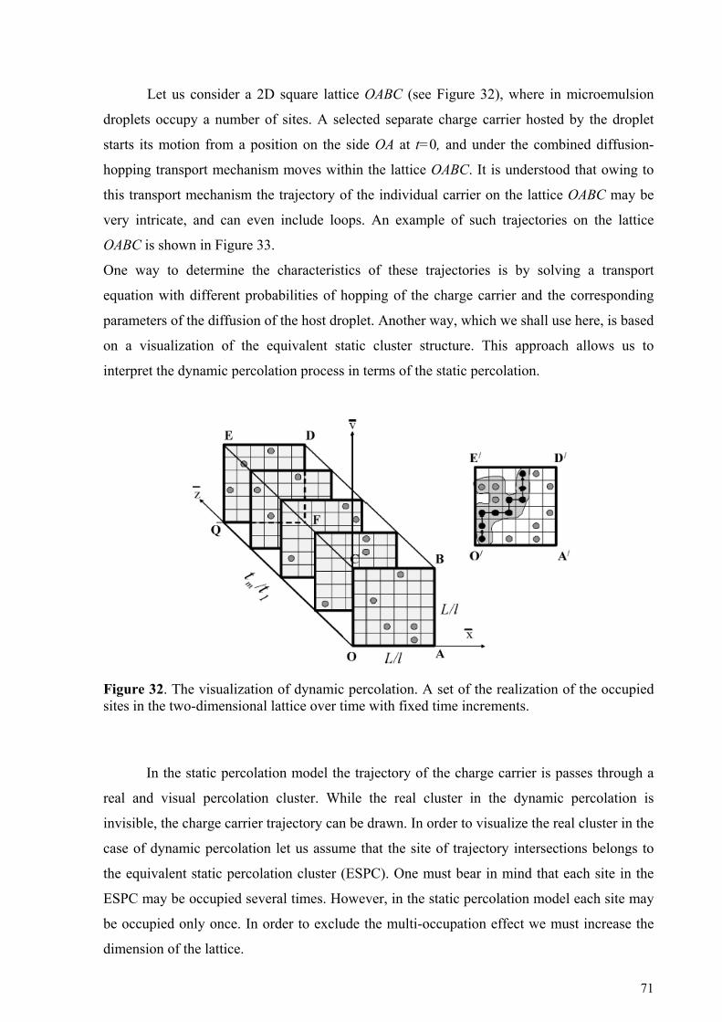
Let us consider a 2D square lattice OABC (see Figure 32), where in microemulsion
droplets occupy a number of sites. A selected separate charge carrier hosted by the droplet
starts its motion from a position on the side OA at t=0, and under the combined diffusion-
hopping transport mechanism moves within the lattice OABC. It is understood that owing to
this transport mechanism the trajectory of the individual carrier on the lattice OABC may be
very intricate, and can even include loops. An example of such trajectories on the lattice
OABC is shown in Figure 33.
One way to determine the characteristics of these trajectories is by solving a transport
equation with different probabilities of hopping of the charge carrier and the corresponding
parameters of the diffusion of the host droplet. Another way, which we shall use here, is based
on a visualization of the equivalent static cluster structure. This approach allows us to
interpret the dynamic percolation process in terms of the static percolation.
Figure 32. The visualization of dynamic percolation. A set of the realization of the occupied sites in the two-dimensional lattice over time with fixed time increments.
In the static percolation model the trajectory of the charge carrier is passes through a
real and visual percolation cluster. While the real cluster in the dynamic percolation is
invisible, the charge carrier trajectory can be drawn. In order to visualize the real cluster in the
case of dynamic percolation let us assume that the site of trajectory intersections belongs to
the equivalent static percolation cluster (ESPC). One must bear in mind that each site in the
ESPC may be occupied several times. However, in the static percolation model each site may
be occupied only once. In order to exclude the multi-occupation effect we must increase the
dimension of the lattice.
71

Figure 33. The charge carrier trajectories in the hyperlattice and the new scale LH/l of the equivalent lattice formation.
A three-dimensional hyperlattice in the hyperspace formed by the spatial and temporal
coordinates corresponds to the two-dimensional square lattice of size L, complemented by the
time axis (see Figure 33). We use non-dimensional spatial coordinates ( lxx =_
and ),
which are normalized by the droplet size l. In turn, the non-dimensional temporal coordinate
(
lyy /_
=
1/ ttz = ) is normalized by the characteristic time t1, which is the time needed for a charge
carrier to move the distance equal to the size of one droplet. Thus the linear non-dimensional
size of the hyperlattice along the two spatial axes is L/l, and the non-dimensional size of the
hyperlattice along the temporal axis is 1ttz mm = . The characteristic time tm corresponds to
the time needed for a charge carrier to visit all the droplets in the maximal cluster sm [150].
Note that the classic SLSP model for a square lattice ABCO would provide a
percolation trajectory connecting opposite sites OA and CB (see Figure 32). On the other
hand, for visualization of dynamic percolation we shall consider an effective three-
dimensional static representation of a percolation trajectory connecting ribs OA and ED
spaced distance LH (see Figure 33). Such a consideration allows us to return to the lattice
OEDA, with the initial dimension d=2, which is non-square and characterized by the two
dimensionless sizes LH/l and L/l. The new lattice size of the system can be determined from
the rectangular triangle OEQ by
72

( ) ( )21
2 ttlLlL mH += , (5.30)
where LH >L. A projection of the three dimensional trajectory on the non-square plane lattice
OADE is shown in Figure 33 by the dotted line. According to the conventional static site
percolation model which always deals with square, cubic, and multidimensional one-scale
lattices, the maximal scale LH/l needs to be chosen in our case as the new scale of a square
lattice (see Figure 33). A transformation from the initial lattice with scale size L/l to the lattice
with the new scale size LH/l may be performed by a renormalization procedure. By the
substitution of scaling relationships (5.23) and (5.24) into (5.30) the expansion coefficient bH
for dynamic percolation can be presented as
⎟⎟⎠
⎞⎜⎜⎝
⎛−
⋅⎟⎟⎠
⎞⎜⎜⎝
⎛+== D
mH
H scc
LLb α
α 1122
1
21.
(5.31)
In the case of dynamic percolation the renormalization condition may be fulfilled
under the conventional condition
1=Ω− DdHb
0=Ω− Dd and under an additional requirement bH=const,
because sm→∞. This is equivalent to the condition const=s Dm
⎟⎠⎞
⎜⎝⎛
α−α
112 and leads to the
relationship 01 =α− D .
Thus, the dynamic HSR is expressed in the form of a system of two equations:
0=⋅Ω− Dd , (5.32)
01 =⋅− Dα . (5.33)
A peculiarity of the dynamic case is the additional equation (5.33) which must be combined
with the static HSR (5.32). After simple transformation, the solution of the system can be
presented in the following way:
α⋅=Ω d . (5.34)
One must bear in mind that the parameter α describes the scaling law (5.24) for the temporal
variable and is equal to the inverse dynamic fractal dimension dD/1=α . Thus, the dynamic
HSR (5.34) can be rewritten as
73

dDd
=Ω
(5.35)
and formally coincides with the HSR (5.29) for the static site percolation model.
Note that the dynamic fractal dimension obtained on the basis of the temporal scaling
law should not necessarily have a value equal to that of the static percolation. We shall show
here that in order to establish a relationship between the static and dynamic fractal dimensions
we must go beyond relationships (5.32) and (5.33) for the scaling exponents.
5.2.3 Relationship between the static and dynamic fractal dimensions
Let us consider the hyperlattice anisotropy coefficient ΘH as the ratio of the
hyperlattice temporal to the spatial scale
( )( )lL
ttmH /
/ 1=Θ.
(5.36)
Taking into account (5.30) and the scaling laws (5.23), (5.24), it is easy to show that when
sm→∞ the validity of the renormalization procedure is similar to the condition that the
extension coefficient bH must be a constant,
consts DmH =⋅Θ=Θ
⎟⎠⎞
⎜⎝⎛
⋅−
αα 11
, (5.37)
where 12 cc=Θ . In the case of dynamic percolation an additional equation (5.33) leads to the
relationship constH =Θ=Θ . In general, Θ≠1 and the hyperlattice is non-cubic as far as the
value of the coefficient Θ depends on the type of dynamics in the complex system.
The validity of (5.37) can be easily proven by an assumption of the existence of the
parameter Θ dependency on the fractal dimension D. The derivation of both parts of (5.37)
with respect to a variable D leads to the differential equation
2m DdDsd ln−=
ΘΘ
. (5.38)
In order to establish the relationship between the static and dynamic fractal dimensions, the
initial conditions of the classical static percolation model must be considered for the solution
74
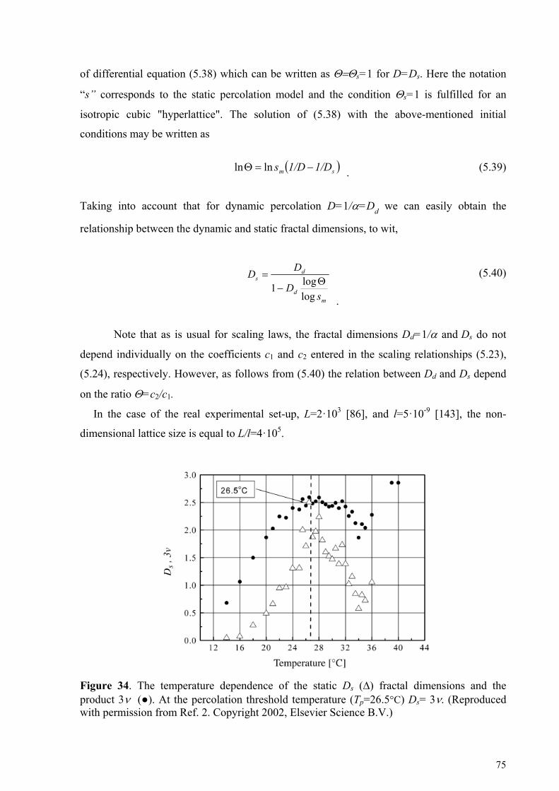
of differential equation (5.38) which can be written as Θ=Θs=1 for D=Ds. Here the notation
“s” corresponds to the static percolation model and the condition Θs=1 is fulfilled for an
isotropic cubic "hyperlattice". The solution of (5.38) with the above-mentioned initial
conditions may be written as
( )sm 1/D1/Ds −=Θ lnln . (5.39)
Taking into account that for dynamic percolation D=1/α=Dd we can easily obtain the
relationship between the dynamic and static fractal dimensions, to wit,
md
ds
sD
DD
loglog1 Θ
−=
.
(5.40)
Note that as is usual for scaling laws, the fractal dimensions Dd=1/α and Ds do not
depend individually on the coefficients c1 and c2 entered in the scaling relationships (5.23),
(5.24), respectively. However, as follows from (5.40) the relation between Dd and Ds depend
on the ratio Θ=c2/c1.
In the case of the real experimental set-up, L=2·103 [86], and l=5·10-9 [143], the non-
dimensional lattice size is equal to L/l=4·105.
Figure 34. The temperature dependence of the static Ds (∆) fractal dimensions and the product 3ν (●). At the percolation threshold temperature (Tp=26.5°C) Ds= 3ν. (Reproduced with permission from Ref. 2. Copyright 2002, Elsevier Science B.V.)
75

Figure 34 shows the temperature dependencies of the static fractal dimensions of the
maximal cluster. Note that at percolation temperature the value of the static fractal dimension
Ds is extremely close to the classical value 2.53 for a three-dimensional lattice in the static site
percolation model [152]. Moreover, the temperature dependence of the stretch parameter ν
(see Figure 34) confirms the validity of our previous result (See (5.11)) ν 3=sD obtained for
the regular fractal model of the percolation cluster [47].
Thus, the non-Debye dielectric behavior in silica glasses, PS and AOT microemulsions, has
similar properties. These systems exhibit an intermediate temperature percolation process that
is associated with the transfer of the electric excitations through the random structures of
fractal paths. It was shown that at the mesoscale range the fractal dimension of the complex
material morphology (Dr for porous glasses and Ds for microemulsions) coincides with the
fractal dimension Dp of the path structure. This value can be evaluated by the fitting of the
experimental DCF to the stretched-exponential relaxation law (2.23).
5.3 Percolation as part of "Strange Kinetic" Phenomena
As shown above, the dielectric percolation phenomena in different systems such as ionic
microemulsions, porous silicon, and porous glasses can actually be analyzed in the framework
of one universal approach based on the idea of electric excitation transport through the fractal
network clusters due to charge carriers’ motion. This model describes the growth of the fractal
pre-percolation clusters. Nevertheless, the model is applicable only to one particular
phenomenon and does not address any basic theories of "strange kinetic" behavior [2].
Obviously, "strange kinetics" is a very wide class of phenomena, which cannot be covered by
the limited number of existing models, and has several distinctive features. Most famous
among these characteristics is the power-law (or stretched exponent) asymptotic with a
fractional exponent for the dipole correlation function in time domain (see (2.23)-(2.25)).
Another property of the percolation as part of a "strange kinetic" is that this class of
phenomena is inherent to many-particle cooperative systems. Such complex matter cannot be
considered as a simple sum of elementary units but rather should be regarded as a whole
system due to the interactions between the elementary components. In a wide sense the word
"interaction" represents not only the interaction with some kind of physical far-ranging field
(say an electromagnetic field) but can also mean a geometrical (or even a quantum) constraint,
or other type of coupling.
76

Since percolation is a property of macroscopic many-particle systems it can be analyzed in
terms of statistical mechanics. The basic idea of statistical mechanics is the relaxation of the
perturbed system to the equilibrium state. In general the distribution function ρ(p,q; t) of a
statistical ensemble depends on the generalized coordinates q, momentum p and time t.
However, in the equilibrium state it does not depend explicitly on time [226-230] and obeys
the equation
0) ;,(
=∂∂ tt
qpρ . (5.41)
The evolution of the distribution function to the equilibrium state is governed by the so-called
Liouville equation (evolution equation)
( ) ( )ti ,,qpρ −=∂
∂ Lt
tq,p,ρ,
(5.42)
where L is the Liouville operator. Thus, by virtue of (5.42) the evolution operator L
determines the dynamical properties of the statistical system. The specific form of this
operator is dependent on the Hamiltonian function H [226-230] as
{ }gHig ,−=L , (5.43)
where {H, g} are the Poisson brackets. In the classical statistical mechanics
∑ ⎟⎟⎠
⎞⎜⎜⎝
⎛∂∂
∂∂
−∂∂
∂∂
=k kkkk q
gpH
pg
qHgH
},{
. (5.44)
In quantum mechanics the functions H, g become operators H and , and obtains the
commutator form
g }ˆ,ˆ{ gH
( HggHih
gH ˆ ˆˆ ˆ2}ˆ,ˆ{ −= )π , where h is the Plank constant.
Therefore, the consistent study of many-particle system dynamics should start by
establishing the H and then solving the evolution equation (5.42). Unfortunately, examples of
such calculations are very rare and are only valid for limited classes of model systems (such
as the Ising model) since these are quite extended calculations. In particular, to the best of our
knowledge, the relaxation patterns (2.23)-(2.25) are as yet not being derived this way. In this
section, we consider the problem from a different side. We will assume that (2.23)-(2.25) are
77
given and try to guess what statistical properties leads to the "strange kinetic" behavior. Let us
first examine the equilibrium state (5.41), whose formal solution gives
constt =) ;,( qpρ . (5.45)
Recently the new concept of fractional time evolution was introduced [45]. In addition to
the usual equilibrium state (5.45), this concept leads to the possibility of the existence of an
equilibrium state with power-law long time behavior. In this case the infinitesimal generator
of time evolution is proportional to the Riemann-Liouville fractional differential
operator . By definition of the Riemann-Liouville fractional differentiation operator
[231,232]
νtD0
( )[ ] ( )[ ] 10,100 ≤<= − ννν thD
dtdthD tt
,
(5.46)
where
( )[ ] ( ) ( ) ( )∫ ≤<′′′−= −−t
t tdtgtttgD0
10 10,1 ν
ννν
Γ (5.47)
is the Riemann-Liouville fractional integration operator and is the
Gamma-function. Obviously, the derivation of order υ should be dependent on the properties
of the cooperative system; although there is no clear understanding for the time being how υ
depends on these properties.
dyyy∫∞
− −=Γ0
1 )exp()( νν
Nevertheless, let us call the "fractional equilibrium state" the state of the statistical system
that under the condition of time independence obeys the following:
0) ;,(0 =tDt qpρυ . (5.48)
We will discuss this state in relation to the recent approaches of the anomalous diffusion
theory [31]. It is well known [226-230] that by virtue of the divergent form of Poisson
brackets (5.44) the evolution of the distribution function ρ(p,q;t) can be regarded as the flow
of a fluid in the phase space. In this interpretation the Liouville equation (5.42) becomes
analogous to the continuity equation for a fluid
78
0) (div
=+
∂∂ vρρ
t , (5.49)
where distribution function ρ is interpreted as the density of a fluid and v is its local velocity.
Let us extend this analogy. The continuity equation accompanied by the relationship between
the gradient of the fluid density and its flux (Darcy's law for the liquid flow or Fourier's law
for heat flow for instance) [233,234]
v )(grad ϑρρ −= (5.50)
gives
ρϑρΔ=
∂∂
t ,
(5.51)
where ϑ is the appropriate constant that characterizes permeability of the space and Δ is the
Laplace differential operator. From a mathematical point of view (5.51) is analogous to the
diffusion equation where ρ is regarded as the density of diffusing particles and ϑ is
proportional to the appropriate diffusion coefficient.
It is well known that the diffusion equation can be obtained in two ways. The first is based
on the equation of continuity and the relationship between the fluid density gradient of its flux
(5.49-5.51). The second way is the probabilistic approach developed from the theory of
Brownian motion [31,226,227,235]. This approach does not appeal to the local differential
equations like (5.49) and (5.50), but considers the probability of jumps between the sites of
some lattice. There is an extension of this approach for the case when the lengths of the jumps
as well as the waiting times between jumps are random. This is the so-called continuous time
random walk (CTRW) scheme [31,236-238]. By applying different probability distribution
functions for waiting time and jump length one can obtain different types of diffusion patterns
[31]. In particular, if the characteristic waiting time diverges because of a long-tailed waiting
time probability distribution function (proportional to t -(1+υ)), but the jump length variance is
still kept finite, then diffusion (5.51) obtains a fractional derivation [31] instead of the first
derivation in time on its left hand side.
ρϑρ υυ Δ= 0 tD . (5.52)
Here the parameter ϑυ has a physical meaning similar to ϑ in (5.51), but with different a
physical dimension. In the general case a term proportional to ρ(t=0) should be added to the
79
right hand side of (5.52) but by choosing the appropriate initial conditions it can be
subtracted. Thus, we will not discuss this term.
Let us reiterate that diffusion defined by (5.51) can be derived using the Brownian motion
approach and a continuity equation. Moreover, one can imply that (5.52), a generalization of
(5.51), can be derived not only in the framework of the CTRW scheme but also by using some
analogy of the continuity equation as well. The difference between (5.51) and (5.52) is only in
time derivation. Thus, the analogy of continuity (5.49) that corresponds to the anomalous
diffusion (5.52) is
0) (div0 =+ υυ ρρ vtD . (5.53)
Let us call it the "anomalous continuity equation". There are two main features that
distinguish this equation from (5.49). The first is that (5.53) becomes non-local in time by
virtue of the convolution form of the fractional derivation operator υtD0 . Second, in spite of
the different physical dimension [m⋅s-υ], the quantity vυ has a physical meaning similar to the
local velocity v.
Let us return back to the Liouville equation that can be regarded as a continuity equation.
There is a possibility to establish an evolution equation not only in the usual form (5.42) but
also based on the anomalous continuity (5.53)
);,() ;,(0 tρLitDt qpqp −=ρυ. (5.54)
This equation implies an equilibrium state in the form (5.48).
Thus, the fractional equilibrium state (5.48) can be considered a consequence of the
anomalous transport of phase points in the phase space that results in the anomalous
continuity (5.53). Note that the usual form of evolution (5.42) is a direct consequence of the
canonical Hamiltonian form of microscopic motion equations. Thus, the evolution of (5.54)
implies that the microscopic equations of motion are not canonical. The actual form of these
equations has not yet been investigated. However, there is great suspicion that in this case
dissipative effects on the microscopic level become important.
If we assume factorization of time dependency in the distribution function then the formal
solution of (5.48) is
80

1
) ;,() ;,(−
⎟⎟⎠
⎞⎜⎜⎝
⎛=
υ
ττρρ
ffff
tt qpqp,
(5.55)
where t ≥ τf, ρf(p,q;τf) and τf depend on the initial conditions. Obviously, the assumption
about factorization of time dependency for the distribution function is not universal. However,
this type of factorization is justified when the equilibrium and non-equilibrium (in the
ordinary sense) parts of distribution function ρ(p,q;t) are orthogonal to each other in the phase
space [230].
The interpretation of any distribution function as a probability density function in the phase
space leads to the requirement
1!
),( 3 =∫∫ NhNddt; qpqpρ
, (5.56)
where 3N is the number of degrees of freedom. This normalization is based on the uncertainty
relation that establishes the minimal phase cell as dpk dqk ≥ h. Substitution of the solution
(5.55) in (5.56) gives
1!
),(1
3 =⎟⎟⎠
⎞⎜⎜⎝
⎛Ξ=
−
∫∫υ
τρ
fNft
hNddt; qpqp
, (5.57)
where is a constant. Thus from (5.57) one can get qpqp ddff∫∫=Ξ );,( τρ
13!−
⎟⎟⎠
⎞⎜⎜⎝
⎛=
Ξ
υ
τ f
N thN
(5.58)
which for υ < 1 indicates a decrease in the number of degrees of freedom.
From one point of view, (5.58) can be interpreted as a manifestation of the non-canonical
nature of the microscopic motion equation and supports the idea of an impact of dissipative
effects on the microscopic level (for time scale t < τf). From another point of view (5.58) can
be related to the "coarse graining" of the phase volume minimal cells. The concept of
fractional evolution is the result of consequent acting of the averaging operator [45]. Each
application of the averaging operator is equal to the loss of information regarding the short
time mobility and is closely associated with the renormalization approach ideas [239].
A simple example of this "coarse graining" is that of two masses in the viscous media
connected by a spring. The spring here represents an interaction between the microscopic
81

particles while viscosity reflects the dissipative effects. Now let us discuss the situation when
one mass is exposed by some mechanical perturbation with a wide spectrum (say the δ-
impulse of force). In the beginning the motions of the masses are almost independent of each
other. The viscosity effect then leads to a decay of the high frequency modes of mobility and
the motions of masses become more and more correlated. At the initial times, one should
observe the motion of two centers of gravity while at the longer time interval it is enough to
know the position of the joint center of gravity. Thus, the "coarse graining" effect leads to a
reduction in the number of degrees of freedom [240].
The reduction of degrees of freedom can also be regarded as the transition from the non-
correlated state to the state with long-range space correlations, and can be accompanied by
phase transition. This is the reason the renormalization approach was used initially to describe
phase transition phenomena [226,228,239]. The theory of the phase transitions investigates
the dependency of macroscopic physical quantities (like sample magnetization or polarization
vectors) on the external parameter (like external fields or temperature) values. The changes of
the degrees of freedom are the result of competition between external perturbations (say
temperature) and internal interactions.
In contrast to phase transitions in the fractional equilibrium state (5.46) the statistical
system loses degrees of freedom during evolution in time. The degrees of freedom,
independent at the short time limit, become dependent later due to the interactions (in the
wide sense coupling, constraint etc.) and dissipative effects. The distribution function for the
fractional equilibrium state (5.55) can be utilized to calculate the macroscopic dipole
correlation function (2.22). The statistical averaging designated <....> in (2.22) is performed
over the equilibrium ensemble (in the usual sense) with a distribution function that does not
depend explicitly on time. If we regard the evolution of the DCF as a fractional equilibrium
state (5.46), then by using properties of statistical averaging and the Liouville operator
[229,230] we can transfer time dependence of the dynamic variable M(t) to time dependence
of the distribution function ρf(p,q;t). Thus, instead of >< )()0( tMM in (2.22) we use
, where subscript f means that statistical averaging was performed with
distribution function (5.55). In this case one will get
f>< )0()0( MM
82

. ,~ )0 ;,()0 ;,()0 ;,( ) ;,()0 ;,()0 ;,(
)0()0()0()0(
)0()0()()0()(
1
ff
f
f
ttddddt
tt
ττρ
ρ
φ
υ
≥⎟⎟⎠
⎞⎜⎜⎝
⎛=
=><
><=
><><
≅
−
∫∫∫∫
qpqpqpMqpMqpqpqpMqpM
MMMM
MMMM
(5.59)
Thus, one can regard the power law dependence of relaxation function (2.24) as a result of the
fractional equilibrium state (5.48).
In order to understand the stretched exponential behavior of DCF (2.23) let us discuss
Gibb's phase exponent )t;,(lnG qpρη −= . This quantity plays a special role in statistical
mechanics and relates to the entropy of the system. If Gibb's exponent obeys fractional
evolution equation
00 =GtD ην, (5.60)
then the distribution function is
⎟⎟⎟
⎠
⎞
⎜⎜⎜
⎝
⎛
⎟⎟⎠
⎞⎜⎜⎝
⎛−=
−1
exp0 ;,() ;,(ν
ηηη τ
ρρ t)t qpqp
,
(5.61)
where ρη(p,q;0) and τη depend on the initial conditions. A calculation analogous to (5.59)
shows that this distribution function leads to the KWW dependency of the DCF. Thus, in the
framework of the fractional time evolution concept the power-law time dependence of the
relaxation function behavior (2.24) and the stretched exponential relaxation (2.23) can be
regarded as two different realizations: the fractal equilibrium state of the distribution function
and the fractal evolution of Gibb's phase exponent.
A similar ideology can also be the basis of the relaxation pattern (2.24) when these two
different types of fractal evolution simultaneously coexist for two subspaces ( p f , q f ) and
( p η , q η ) of the total statistical system phase space ( p, q ). In this case the total distribution
function ρ fη (p,q;t) is the product of two statistically independent distribution functions
ρf( p f , q f ;t) and ρη( p η , q η ;t)
⎟⎟⎟
⎠
⎞
⎜⎜⎜
⎝
⎛
⎟⎟⎠
⎞⎜⎜⎝
⎛−⎟
⎟⎠
⎞⎜⎜⎝
⎛=
−− 11
exp);,()0 ;,(),(ν
η
υ
ηηηη τττρρρ ttt;
ffff ff qpqpqp
,
(5.62)
that can be related to the relaxation pattern (2.24).
83

The relaxation law (5.62) has been observed in the case of dynamic percolation in ionic
micro-emulsions (see section 5.2). Below the percolation threshold, the relaxation process is
provided by two types of mobility: mobility of the pre-percolation clusters and mobility of the
charge carriers inside these clusters. The first type of mobility is governed by the power-law
(2.23) while the second type exhibits stretched exponential behavior (2.22) [152]. Thus, there
are two subspaces of degrees of freedom: the first is related to the mobility of pre-percolation
clusters as a whole and the second reflects the mobility inside the clusters. Approaching the
percolation threshold pre-percolation clusters grow and become an infinite (or very large for a
real finite size system) percolation cluster at the threshold. At this point mobility of the cluster
is impossible, as first subspaces of degrees of freedom disappear and the relaxation function
obtains the stretched exponential pattern (2.22). Far from the percolation, one finds the
opposite situation. The pre-percolation clusters are small, second subspace degrees of freedom
are not yet developed and the relaxation function obeys the power-law (2.23).
In this section we made an attempt to interpret our main results in static and dynamic
percolation in terms of statistical mechanics and to find the link to several other approaches
and models that have describe different aspects of "strange kinetic" phenomena. Obviously,
the arguments represented in this section are not rigorous. They are hints rather than the
proofs. Nevertheless, our attempts to find a unified ideology can result in a deeper
understanding of the statistical background of “strange kinetics” and to draw the following
general picture.
As we have discussed above, the non-canonical nature of the motion on the microscopic
level can be considered as the initial basis of “strange kinetics“. In general, this non-canonical
motion of one elementary microscopic unit reflects the cooperativity due to the different kinds
of interaction in the statistical many particles ensembles. Such interactions, which are specific
for each complex system, lead to energy dissipation and can be reduced to the integral term
associated with the memory effect in the different kinds of evolution equations. For any
processes, which display scaling properties (such as percolation, or phase transition), the non-
canonical motion can be described in terms of the fractional Liouville equation (5.54).
According to the integral representation of the fractional derivation by (5.46) and (5.47) the
scaling properties are contained in the kernel of the convolution integral. As was shown the
fractional Liouville equation can be considered as the base equation for different approaches
and models (percolation, anomalous diffusion, damping oscillations, renormalization
approach, etc).
84

5.4 Universal scaling behavior in H-bonding networks
The properties of H-bonded liquids were already reviewed earlier in section 4.4. Here
we would like to continue the consideration of these samples this time with regard to their
universal scaling behavior. We have separated this discussion into two parts, which consider
two different kinds of glycerol-water mixtures.
5.4.1 Glycerol-rich mixtures
The analyses of the master plots presented in Figure 27 in the glycerol rich region showed that
the use of known phenomenological relations and their superposition for the simultaneous
fitting of the EW, the main process and dc-conductivity provide satisfactory results only with
a significant number of fitting parameters. Therefore, we propose a new phenomenological
function with a lesser number of fitting parameters as follows:
( ) ( )[ ]( ) ωτε
εωτ
ωτεεωε β0
*
11
iB
iA q Δ
+++⋅Δ
=− ∞
, (5.63)
where τεσ /Δ= B is the dc-conductivity, B is a constant, β is a parameter describing
asymmetrical relaxation peak broadening (similar to βCD), and A and q are parameters to
describe the EW, respectively [208]. For glycerol-water mixtures in the present temperature-
and concentration-range:
γβ +−= 1q , (5.64)
where γ is equal to 0.08 for the entire range of the observed concentrations. The nature of this
parameter is not clear yet. Figure 35 shows a good fitting of both real and imaginary parts of
the raw dielectric spectra using relationship (5.63).
Moreover this fitting shows that in the considered temperature-frequency landscape
only the temperature dependence of ( )Tεε Δ=Δ and ( )Tττ = are observed, while the other
parameters B, β, A, and q are not temperature dependent. Thus, the proposed
phenomenological model (5.63) as a modification of the CD function (2.21) with a
conductivity term could be successfully applied for simultaneous fitting of dc-conductivity,
the main process and the EW presented in the master plots (see Figure 27). At the same time,
parameters β, A and q have a concentration dependence where A and β decrease with a
decrease of glycerol content (Figure 36), while parameter q increases according to (5.64).
85
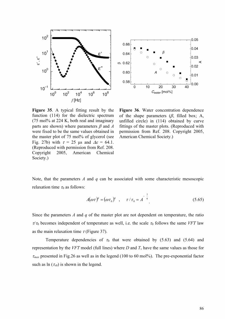
Figure 35. A typical fitting result by the function (114) for the dielectric spectrum (75 mol% at 224 K, both real and imaginary parts are shown) where parameters β and A were fixed to be the same values obtained in the master plot of 75 mol% of glycerol (see Fig. 27b) with τ = 25 μs and Δε = 64.1. (Reproduced with permission from Ref. 208. Copyright 2005, American Chemical Society.)
Figure 36. Water concentration dependence of the shape parameters (β, filled box; A, unfilled circle) in (114) obtained by curve fittings of the master plots. (Reproduced with permission from Ref. 208. Copyright 2005, American Chemical Society.)
Note, that the parameters A and q can be associated with some characteristic mesoscopic
relaxation time τ0 as follows:
( ) ( )qqA 0ωτωτ = , qA1
0/−
=ττ . (5.65)
Since the parameters A and q of the master plot are not dependent on temperature, the ratio
τ/τ0 becomes independent of temperature as well, i.e. the scale τ0 follows the same VFT law
as the main relaxation time τ (Figure 37).
Temperature dependencies of τ0 that were obtained by (5.63) and (5.64) and
representation by the VFT model (full lines) where D and Tv have the same values as those for
τmax presented in Fig.26 as well as in the legend (100 to 60 mol%). The pre-exponential factor
such as ln (τv0) is shown in the legend.
86
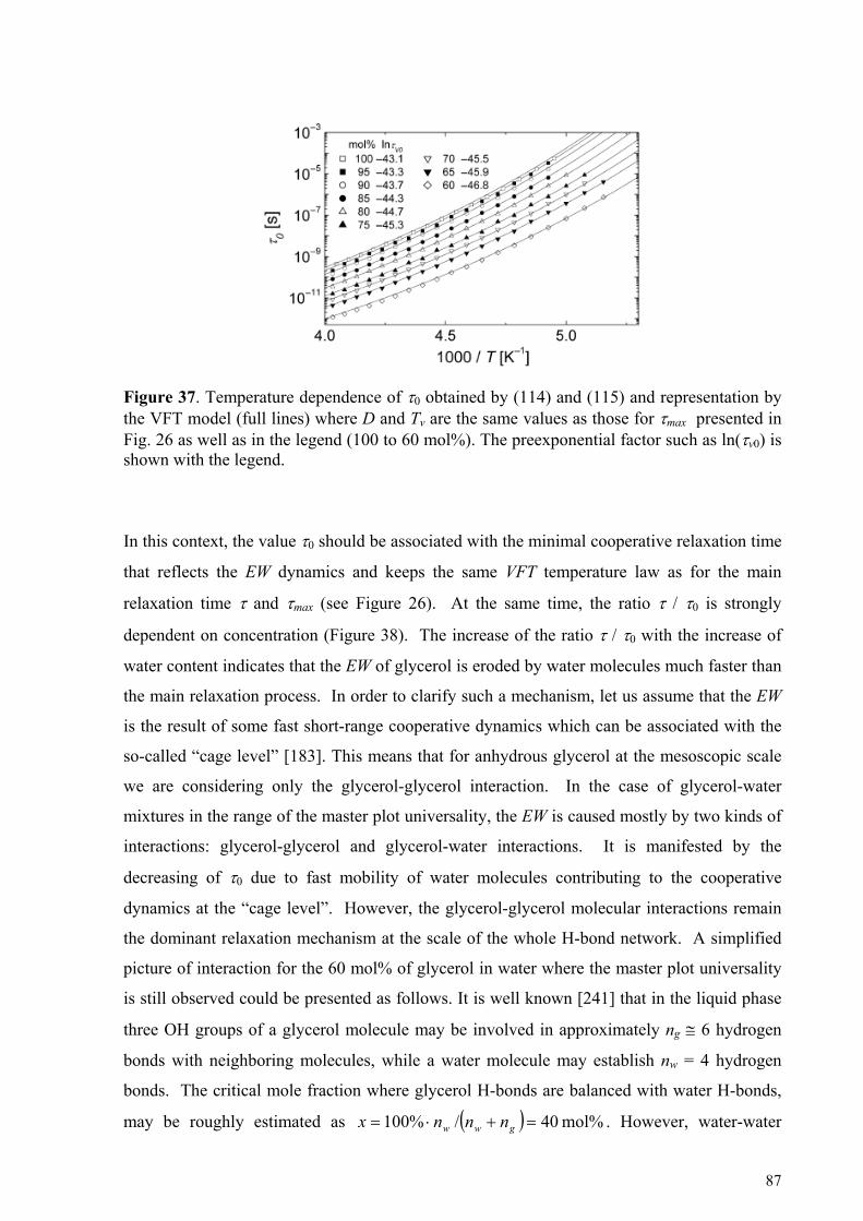
Figure 37. Temperature dependence of τ0 obtained by (114) and (115) and representation by the VFT model (full lines) where D and Tv are the same values as those for τmax presented in Fig. 26 as well as in the legend (100 to 60 mol%). The preexponential factor such as ln(τv0) is shown with the legend.
In this context, the value τ0 should be associated with the minimal cooperative relaxation time
that reflects the EW dynamics and keeps the same VFT temperature law as for the main
relaxation time τ and τmax (see Figure 26). At the same time, the ratio τ / τ0 is strongly
dependent on concentration (Figure 38). The increase of the ratio τ / τ0 with the increase of
water content indicates that the EW of glycerol is eroded by water molecules much faster than
the main relaxation process. In order to clarify such a mechanism, let us assume that the EW
is the result of some fast short-range cooperative dynamics which can be associated with the
so-called “cage level” [183]. This means that for anhydrous glycerol at the mesoscopic scale
we are considering only the glycerol-glycerol interaction. In the case of glycerol-water
mixtures in the range of the master plot universality, the EW is caused mostly by two kinds of
interactions: glycerol-glycerol and glycerol-water interactions. It is manifested by the
decreasing of τ0 due to fast mobility of water molecules contributing to the cooperative
dynamics at the “cage level”. However, the glycerol-glycerol molecular interactions remain
the dominant relaxation mechanism at the scale of the whole H-bond network. A simplified
picture of interaction for the 60 mol% of glycerol in water where the master plot universality
is still observed could be presented as follows. It is well known [241] that in the liquid phase
three OH groups of a glycerol molecule may be involved in approximately ng ≅ 6 hydrogen
bonds with neighboring molecules, while a water molecule may establish nw = 4 hydrogen
bonds. The critical mole fraction where glycerol H-bonds are balanced with water H-bonds,
may be roughly estimated as ( ) mol% 40/%100 =+⋅= gww nnnx . However, water-water
87
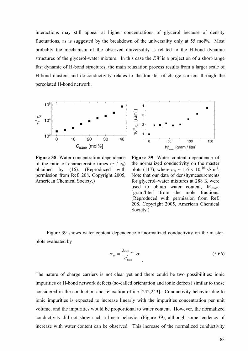
interactions may still appear at higher concentrations of glycerol because of density
fluctuations, as is suggested by the breakdown of the universality only at 55 mol%. Most
probably the mechanism of the observed universality is related to the H-bond dynamic
structures of the glycerol-water mixture. In this case the EW is a projection of a short-range
fast dynamic of H-bond structures, the main relaxation process results from a larger scale of
H-bond clusters and dc-conductivity relates to the transfer of charge carriers through the
percolated H-bond network.
Figure 38. Water concentration dependence of the ratio of characteristic times (τ / τ0) obtained by (16). (Reproduced with permission from Ref. 208. Copyright 2005, American Chemical Society.)
Figure 39. Water content dependence of the normalized conductivity on the master plots (117), where σm ~ 1.6 × 10⁻¹⁶ sSm-1. Note that our data of densitymeasurements for glycerol–water mixtures at 288 K were used to obtain water content, Wwater, [gram/liter] from the mole fractions. (Reproduced with permission from Ref. 208. Copyright 2005, American Chemical Society.)
Figure 39 shows water content dependence of normalized conductivity on the master-
plots evaluated by
σεπτ
σ "max
max2=m
. (5.66)
The nature of charge carriers is not clear yet and there could be two possibilities: ionic
impurities or H-bond network defects (so-called orientation and ionic defects) similar to those
considered in the conduction and relaxation of ice [242,243]. Conductivity behavior due to
ionic impurities is expected to increase linearly with the impurities concentration per unit
volume, and the impurities would be proportional to water content. However, the normalized
conductivity did not show such a linear behavior (Figure 39), although some tendency of
increase with water content can be observed. This increase of the normalized conductivity
88
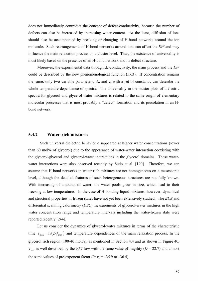
does not immediately contradict the concept of defect-conductivity, because the number of
defects can also be increased by increasing water content. At the least, diffusion of ions
should also be accompanied by breaking or changing of H-bond networks around the ion
molecule. Such rearrangements of H-bond networks around ions can affect the EW and may
influence the main relaxation process on a cluster level. Thus, the existence of universality is
most likely based on the presence of an H-bond network and its defect structure.
Moreover, the experimental data through dc-conductivity, the main process and the EW
could be described by the new phenomenological function (5.63). If concentration remains
the same, only two variable parameters, Δε and τ, with a set of constants, can describe the
whole temperature dependence of spectra. The universality in the master plots of dielectric
spectra for glycerol and glycerol-water mixtures is related to the same origin of elementary
molecular processes that is most probably a “defect” formation and its percolation in an H-
bond network.
5.4.2
)
Water-rich mixtures
Such universal dielectric behavior disappeared at higher water concentrations (lower
than 60 mol% of glycerol) due to the appearance of water-water interaction coexisting with
the glycerol-glycerol and glycerol-water interactions in the glycerol domains. These water-
water interactions were also observed recently by Sudo et al. [190]. Therefore, we can
assume that H-bond networks in water rich mixtures are not homogeneous on a mesoscopic
level, although the detailed features of such heterogeneous structures are not fully known.
With increasing of amounts of water, the water pools grow in size, which lead to their
freezing at low temperatures. In the case of H-bonding liquid mixtures, however, dynamical
and structural properties in frozen states have not yet been extensively studied. The BDS and
differential scanning calorimetry (DSC) measurements of glycerol-water mixtures in the high
water concentration range and temperature intervals including the water-frozen state were
reported recently [244].
Let us consider the dynamics of glycerol-water mixtures in terms of the characteristic
time ( maxmax 2/1 fπτ = and temperature dependences of the main relaxation process. In the
glycerol rich region (100-40 mol%), as mentioned in Section 4.4 and as shown in Figure 40,
maxτ is well described by the VFT law with the same value of fragility (D = 22.7) and almost
the same values of pre-exponent factor ( vτln = –35.9 to –36.4).
89
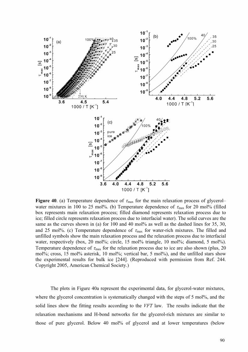
Figure 40. (a) Temperature dependence of τmax for the main relaxation process of glycerol–water mixtures in 100 to 25 mol%. (b) Temperature dependence of τmax for 20 mol% (filled box represents main relaxation process; filled diamond represents relaxation process due to ice; filled circle represents relaxation process due to interfacial water). The solid curves are the same as the curves shown in (a) for 100 and 40 mol% as well as the dashed lines for 35, 30, and 25 mol%. (c) Temperature dependence of τmax for water-rich mixtures. The filled and unfilled symbols show the main relaxation process and the relaxation process due to interfacial water, respectively (box, 20 mol%; circle, 15 mol% triangle, 10 mol%; diamond, 5 mol%). Temperature dependence of τmax for the relaxation process due to ice are also shown (plus, 20 mol%; cross, 15 mol% asterisk, 10 mol%; vertical bar, 5 mol%), and the unfilled stars show the experimental results for bulk ice [244]. (Reproduced with permission from Ref. 244. Copyright 2005, American Chemical Society.)
The plots in Figure 40a represent the experimental data, for glycerol-water mixtures,
where the glycerol concentration is systematically changed with the steps of 5 mol%, and the
solid lines show the fitting results according to the VFT law. The results indicate that the
relaxation mechanisms and H-bond networks for the glycerol-rich mixtures are similar to
those of pure glycerol. Below 40 mol% of glycerol and at lower temperatures (below
90

~230 K), the temperature dependence of the maxτ was continuously changed from VFT to
Arrhenius shape, as shown in Figure 40a (dashed lines). Our analyses and comparison with
the literature [190] shows that maxτ temperature behavior in the water-rich region can depend
on the temperature history, although no differences were found in glycerol-rich regions above
Tg (here Tg is the glass transition temperature). These results may indicate that mesoscopic
structures of H-bond networks in glycerol-rich regions are quite homogeneous. In contrast, in
water-rich regions, such mixtures have a more complicated dynamic behavior. Glycerol
molecules cannot provide all water molecules with H-bond networks, and correspondingly the
system forms so-called glycerol and water cooperative domains, respectively. Dynamic
structures of such domains can depend on the temperature hysteresis. The critical molar
fraction (xg) would then relate to the number of H-bonds of glycerol and would be
approximately 40 mol% as it was shown above (See Section 5.4.1).
The existence of this critical concentration of 40 mol% of glycerol is well supported
by the results obtained from further study of the water-rich region. Figure 40b shows the
temperature dependence of maxτ for 20 mol% of glycerol. At lower temperatures, maxτ
demonstrates a behavior similar to that of higher glycerol concentrations. However, when the
temperature was increased and approached T = 206 K, a crystallization of the extra water
occurred and maxτ increased up to nearly the same vales as that of 35 mol% of glycerol. After
the crystallization, two additional Arrhenius type relaxation processes were observed (Figure
41 shows the typical dielectric spectra of before- and after- the crystallization). One of these
relaxation processes is due to the presence of ice cores, since the relaxation time and its
activation energy (~ 77 kJ / mol) is similar to the well known values for bulk ice which were
reported by Auty and Cole [245] (Figure 40c). Another relaxation process may relate to the
presence of some interfacial water between the ice core and the mesoscopic glycerol- water
domain. The glycerol concentration of this domain was enriched up to the critical
concentration ~40 mol% by the freezing of the extra water that was free from the glycerol H-
bond networks.
In the cases of 15-, 10-, and 5- mol% of glycerol-water mixtures, the ice cores have
already been formed during the quenching down to the starting temperature of the BDS
measurements and maxτ of the main relaxation process for all these mixtures shows values that
are similar to those of 35 or 40 mol% glycerol-water mixtures (see Figure 40c). Furthermore,
the two additional relaxation processes (due to ice and interfacial water) also traced the same
91
Figure 41. Typical dielectric spectra of 20 mol% of glycerol—water mixtures at (a) 185 K (supercooled state) and (b) 218 K (frozen state), where solid and dashed curves show the real and imaginary parts of complex dielectric permittivity. Each relaxation process in the frozen state was fitted by (114) and by Cole–Cole and Debye relaxation functions, respectively, in order to separate the main process, the process due to interfacial water, and the process due to ice. (Reproduced with permission from Ref. 244. Copyright 2005, American Chemical Society.)
lines, respectively. It is worth noting that the activation energy of ~33 kJ/mol of the
relaxation process resulting from interfacial water is similar to the reported values ~28 kJ/mol
for bound water on protein-surfaces in aqueous solutions [246] and ~30-40 kJ/mol for surface
water on porous glasses, depending on the porous glass preparation [256]. The relaxation time
for this interfacial water is ~100 times larger than that for the bound water reported in protein
solutions [246]. In the case of bound water in protein solutions, this interfacial water is
surrounded by fast-mobile water molecules from the solvent. In the case of the water-rich
glycerol-water mixtures the interfacial water molecules would be confined between two slow
regions such as the ice and glycerol-water domains, therefore, mobility of the interfacial water
in water-glycerol mixtures would be highly restricted.
The glass transition temperature (Tg), which is defined as the temperature where the
relaxation time is 100 sec [247,248], was evaluated for glycerol-water mixtures using
92

Figure 42. (a) Glycerol concentration dependence of the glass-transition temperature obtained by DSC measurements (filled box represnts supercooled state, unfilled box represents frozen state) and by BDS data (filled circle) (b) Typical raw data of DSC measurements (10 mol% of glycerol), where the glass transition and a broad melting behavior were observed. (Reproduced with permission from Ref. 244. Copyright 2005, American Chemical Society.)
Figure 43. Glycerol concentration dependence of dc-conductivity (filled box represents supercooled state at 209 K, filled circle represents frozen state at 209 K, open box represents supercooled state at 212 K, open circle represents frozen state at 212 K, filled diamond represents supercooled state at 215 K, and filled triangle represents frozen state at 215 K). (Reproduced with permission from Ref. 244. Copyright 2005, American Chemical Society.)
temperature dependencies of maxτ for the main dielectric relaxation process (See Figure 40a).
As shown in Figure 42a, the glass transition temperatures (Tg) obtained by DSC
measurements were in good agreement with BDS data. It is worth pointing out that Tg for 2.5-,
10-, and 15- mol% of glycerol-water mixtures in the frozen state all have the same values as
the Tg for 40 mol% of the glycerol-water mixture. This result indicates that the glass transition
observed in frozen state results from the mesoscopic glycerol-water domains of 40 mol%
glycerol. Moreover, even simple dc-conductivity data obtained by BDS at particular
temperatures show concentration independent behaviors in the frozen state, and the values are
close to that of 40- or 35- mol% of glycerol (Figure 43). Note that these results support the
hypothesis that the mechanism of dc-conductivity in a supercooled state is most likely that of
defect translocation as discussed recently [208], possible because the increase of ionic
impurities did not affect the frozen state as shown in Figure 43.
In order to estimate the ratio between the amounts of water in the mesoscopic
glycerol-water domains, interfacial water and ice in glycerol-water mixtures, one can use the
melting-enthalpy ΔH obtained from DSC data. Note that in this specific case, the total
93
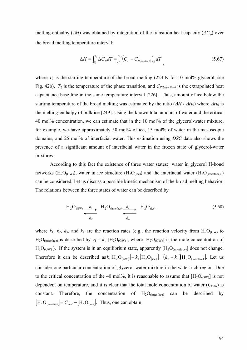
melting-enthalpy (ΔH) was obtained by integration of the transition heat capacity (ΔCP) over
the broad melting temperature interval:
( )( )∫∫ −=Δ=Δ2
1
2
1)
T
T pbaselinePP
T
T P dTCCdTCH,
(5.67)
where T1 is the starting temperature of the broad melting (223 K for 10 mol% glycerol, see
Fig. 42b), T2 is the temperature of the phase transition, and CP(base line) is the extrapolated heat
capacitance base line in the same temperature interval [226]. Thus, amount of ice below the
starting temperature of the broad melting was estimated by the ratio (ΔH / ΔH0) where ΔH0 is
the melting-enthalpy of bulk ice [249]. Using the known total amount of water and the critical
40 mol% concentration, we can estimate that in the 10 mol% of the glycerol-water mixture,
for example, we have approximately 50 mol% of ice, 15 mol% of water in the mesoscopic
domains, and 25 mol% of interfacial water. This estimation using DSC data also shows the
presence of a significant amount of interfacial water in the frozen state of glycerol-water
mixtures.
According to this fact the existence of three water states: water in glycerol H-bond
networks (H2O(GW)), water in ice structure (H2O(ice)) and the interfacial water (H2O(interface) )
can be considered. Let us discuss a possible kinetic mechanism of the broad melting behavior.
The relations between the three states of water can be described by
(ice)2)(interface2(GW)2 OH OH OH , (5.68) k1 3
k2 4
k
k
where k1, k2, k3, and k4 are the reaction rates (e.g., the reaction velocity from H2O(GW) to
H2O(interface) is described by v1 = k1 [H2O(GW)], where [H2O(GW)] is the mole concentration of
H2O(GW) ). If the system is in an equilibrium state, apparently [H2O(interface)] does not change.
Therefore it can be described as ( )[ ] ( )[ ] ( ) ( )[ ]interface232ice24GW21 OHOHOH kkkk +=+ . Let us
consider one particular concentration of glycerol-water mixture in the water-rich region. Due
to the critical concentration of the 40 mol%, it is reasonable to assume that [H2O(GW)] is not
dependent on temperature, and it is clear that the total mole concentration of water (Ctotal) is
constant. Therefore, the concentration of H2O(interface) can be described by
( )[ ] ( )[ ]ice2interface2 OHOH −= totalC . Thus, one can obtain:
94
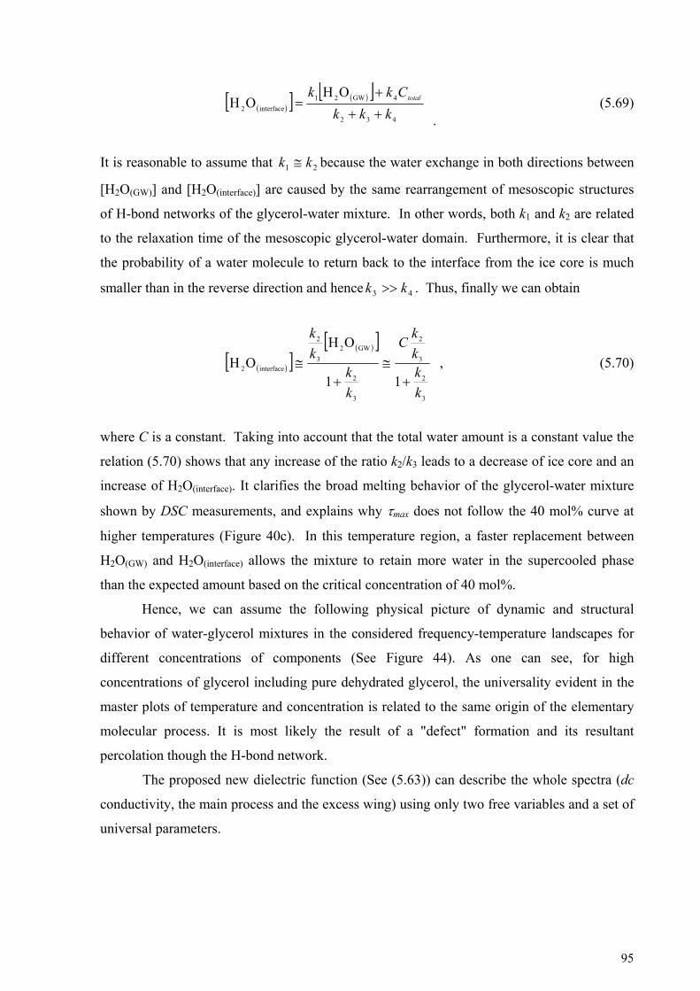
( )[ ] ( )[ ]432
4GW21interface2
OHOH
kkkCkk total
++
+=
. (5.69)
It is reasonable to assume that 21 kk ≅ because the water exchange in both directions between
[H2O(GW)] and [H2O(interface)] are caused by the same rearrangement of mesoscopic structures
of H-bond networks of the glycerol-water mixture. In other words, both k1 and k2 are related
to the relaxation time of the mesoscopic glycerol-water domain. Furthermore, it is clear that
the probability of a water molecule to return back to the interface from the ice core is much
smaller than in the reverse direction and hence . Thus, finally we can obtain 43 kk >>
( )[ ]( )[ ]
3
2
3
2
3
2
GW23
2
interface2
11
OHOH
kkkk
C
kk
kk
+≅
+≅ , (5.70)
where C is a constant. Taking into account that the total water amount is a constant value the
relation (5.70) shows that any increase of the ratio k2/k3 leads to a decrease of ice core and an
increase of H2O(interface). It clarifies the broad melting behavior of the glycerol-water mixture
shown by DSC measurements, and explains why τmax does not follow the 40 mol% curve at
higher temperatures (Figure 40c). In this temperature region, a faster replacement between
H2O(GW) and H2O(interface) allows the mixture to retain more water in the supercooled phase
than the expected amount based on the critical concentration of 40 mol%.
Hence, we can assume the following physical picture of dynamic and structural
behavior of water-glycerol mixtures in the considered frequency-temperature landscapes for
different concentrations of components (See Figure 44). As one can see, for high
concentrations of glycerol including pure dehydrated glycerol, the universality evident in the
master plots of temperature and concentration is related to the same origin of the elementary
molecular process. It is most likely the result of a "defect" formation and its resultant
percolation though the H-bond network.
The proposed new dielectric function (See (5.63)) can describe the whole spectra (dc
conductivity, the main process and the excess wing) using only two free variables and a set of
universal parameters.
95
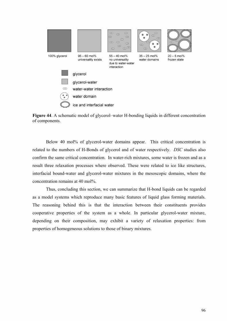
Figure 44. A schematic model of glycerol–water H-bonding liquids in different concentration of components.
Below 40 mol% of glycerol-water domains appear. This critical concentration is
related to the numbers of H-Bonds of glycerol and of water respectively. DSC studies also
confirm the same critical concentration. In water-rich mixtures, some water is frozen and as a
result three relaxation processes where observed. These were related to ice like structures,
interfacial bound-water and glycerol-water mixtures in the mesoscopic domains, where the
concentration remains at 40 mol%.
Thus, concluding this section, we can summarize that H-bond liquids can be regarded
as a model systems which reproduce many basic features of liquid glass forming materials.
The reasoning behind this is that the interaction between their constituents provides
cooperative properties of the system as a whole. In particular glycerol-water mixture,
depending on their composition, may exhibit a variety of relaxation properties: from
properties of homogeneous solutions to those of binary mixtures.
96

5.5 Liquid-like behavior in doped ferroelectric crystals
In the previous section we considered in detail the behavior of liquid glass forming
substances. However, such liquid-like behavior can be also inherent to the dielectric
properties of crystalline samples.
Now let us discuss such behavior as was recently observed in doped ferroelectric
crystals in the paraelectric phase (See Section 4.3). As Process B was observed only in crystal
#1 (see Figure 18) it must be attributed to the presence of the Cu impurities embedded at
random in the KTN crystal. The Arrhenius nature of the process at elevated temperatures
above 354 K indicates normal relaxation of the independent Cu+ ions [179]. These ions are
significantly smaller than the K+ sites in which they reside (The radii of the Cu+ and the K+
ions are 0.77 Ǻ and 1.52 Ǻ respectively [250]), leading to off-center displacements. The Cu+
ions can therefore hop between the eight symmetrical minima of their potential wells. Indeed,
the energy of activation of corresponds to the activation energies for the
hopping of transition metal ion impurities in KTaO3 [251].
eVE Ba 37.0=
VFT behavior has been noted in crystal systems with a dipole glass phase [176].
However the VFT behavior in crystal #1 is related to the relaxation of the Cu+ ions in the
paraelectric phase and is more akin to relaxations in glass forming liquids [179]. The
formulism of Adam and Gibbs [63] (A&G) has been successfully applied to such systems.
According to the A & G theory, this behavior originates from the cooperative rearrangement
of some clusters. It is well established that in KTN crystals in the paraelectric phase the Nb+5
ions are displaced from the center of inversion of the unit cells [172]. These displacements
form dipolar clusters with a correlation length that increases as the system is cooled towards
the ferroelectric phase transition. We propose that the cooperative relaxation observed at
T<354 K is produced by the interaction between such dipolar clusters that form around the
relaxing Cu+ ions, and that act as the rearranging clusters in the A & G model. Adopting the
formalism of A & G [63] the minimum cluster size z, is related to the rate of relaxation P(T,z)
by
⎟⎟⎠
⎞⎜⎜⎝
⎛ Δ−∝
TkzzTP
B
μexp),( . (5.71)
VFT behavior is obtained by equating VFTTT
Tz−
= and noting that VFTE=Δμ [65]. Fitting
the VFT model to the experimental results of τB in the paraelectric phase gives TVFT=228 and
97
Δμ=0.02 eV. Identifying the temperature at which τB deviates from the Arrhenius model with
the onset of cooperativity yields a minimum cluster size given by
8.2=−
=kx
x
TTTz . (5.72)
This coincides well with an estimation of the minimum size of the dipolar cluster formed
around nearest neighbors Nb+5 ion given by [ ] [ ] 63.238.0 115 ≈= −−+Nb . At elevated
temperatures (T>354 K), the Nb+5 ions hop at random between equivalent minima of their
potential wells within their site in the unit cell. As the phase transition is approached these
ions form a dipolar cluster around the Cu+ ions that are randomly distributed far apart from
each other. These clusters are at first of a minimum size containing only the Nb+5 ions that
are closest to the Cu+ ion. As the phase transition is approached further the cluster size
around the Cu+ ion grows accordingly. These represent the rearranging clusters of the A & G
theory.
An independent assessment of the validity of the A & G interpretation to the Cu+
induced relaxation (Process B) was provided by direct estimation of the configurational
entropy at the ferroelectric phase transition. The phase transition is dominated by a shift in the
position of the Nb5+ ion in relation to the lattice. The coupling between the Cu+ ions and the
Nb5+ polar clusters, evident in the paraelectric phase, will further contribute to the
configuational entropy of the phase transition.
It is well known that the configurational entropy can be evaluated from the heat
capacitance of the crystal, derived from DSC measurements, by the integral
( ) ( )[ ] )(ln)(ln2
1
ln
ln
TdbaselineCTCTST
TppC ∫ −=Δ , (5.73)
where T1 is the onset and T2 is the completion of the phase transition, and CP(baseline) is the
extrapolated baseline heat capacitance in the temperature interval [226]. The results for the
pure KTN crystal (#2) and the Cu-doped KTN crystal (#1) are presented in Figure 45. The
resulting difference was found to be ΔS= 0.79×10⁻³Jg-1. Normalized to the Cu+ -ion content
we have per Cu+ -ion ΔSCu = 2.068×10⁻²¹J ≈ 0.013 eV. This result is in a good agreement
with Δμ = 0.02 eV derived from fitting the VFT model to τB(T), given the spatial variation of
the Cu concentration in the crystal.
98

Figure 45. The configurational entropies of the ferroelectric phase transition for crystals #1 (Δ) and #2 (+). The difference in entropy between the two crystals, ΔS, is 0.79 ×10⁻³ Jg-1 and this is assigned to the Cu+ dopants. The DSC measurements were made with the cooling and heating rates 5 K/min in an interval ranging from 373 K to 220 K using a DSC 2920 calorimeter (TA Instruments) [179]. (Reproduced with permission from Ref. 179. Copyright 2004, The American Physical Society.)
At the onset of the ferroelectric phase transition the Cu+ ions are frozen and no longer
constitute the seed of the relaxation process. In this respect the ferroelectric phase transition
“quenches” the glass-forming liquid. Below the phase transition temperature, the dipolar
clusters surrounding the Nb5+ ions merge to yield the spontaneous polarization of the (now
ferroelectric) crystal, and due to the strong crystal field, the off-center potential minima of the
Cu+ ions are no longer symmetrical.
Thus, one may summarize the physical picture of the relaxation dynamics in KTN
crystal doped with Cu+-ions in the following way: In the paraelectric phase, as the
ferroelectric phase transition is approached, the Nb5+ ions form dipolar clusters around the
randomly distributed Cu+ impurity ions. The interaction between these clusters gives rise to a
cooperative behavior according to the AG theory of glass-forming liquids. At the ferroelectric
phase transition the cooperative relaxation of the Cu+ -ions is effectively “frozen.”
99

5.6 Relaxation Kinetics of Confined Systems
It was already mentioned in Section 2.3 of this paper that kinetics associated with
relaxation parameters measured by dielectric spectroscopy can provide significant information
about the substance under study. Even without the quantitative data, having only qualitative
information, one can, for example, identify a glassy material by non liner VFT relaxation time
dependence. In this section we will discuss another type of relaxation kinetics which is
associated with confined systems and we will illustrate this type using some experimental
examples.
5.6.1 Model of relaxation kinetics for confined systems
The model we utilize here, was first introduced to describe the relaxation properties of water
adsorbed on the inner surfaces of porous glasses [155] and which was then reviewed in [78].
The main idea of this model is that the relaxation kinetics in this case is provided in this case
by a process that must satisfy two statistically independent conditions. Thus, if one assigns the
probability to satisfy the first condition and to satisfy the second condition, then the
probability
1p 2p
p for a relaxation act to occur in such a system is
21 ppp = . (5.74)
Let us discuss a system, which consists of a number of particles where their relaxation is
provided by the reorientations (a jump or another type of transition) of particles between two
local equilibrium states. In the spirit of the Arrhenius model (2.26), the first requirement for
the relaxation is that the particles have enough energy to overcome the potential barrier
between the states of local equilibrium for the elementary constituents of the system under
consideration. Thus,
aE
⎟⎟⎠
⎞⎜⎜⎝
⎛−=
TkEpB
aexp1
. (5.75)
The essential idea of the new model is that is the probability that there will be enough free
volume, , in the vicinity of a relaxing particle with its own volume, , to allow
reorientation [69,70,78,155]. In other words we imply that in order to participate in a
relaxation a particle must have a ‘defect’ in its vicinity. Then,
2p
fv 0v
100

⎟⎟⎠
⎞⎜⎜⎝
⎛−=
fvvp 0
2 exp . (5.76)
In itself this probability represents a kind of constraint for the entire relaxation process and
slows down the relaxation. Combining (5.73)-(5.76) and taking into account the relationship
p/1~τ the following expression can be obtained:
fB
a
vv
TkE 0
0
ln +=⎟⎟⎠
⎞⎜⎜⎝
⎛ττ
. (5.77)
As mentioned earlier in Section 2.3 it is usually assumed that free volume grows with
increasing temperature. This idea reflects thermal expansion, i.e. if the number of relaxing
particles in the system is kept constant, then the thermal expansion leads to an increase of free
volume with temperature growth. However, this assumption may be wrong for the case of the
confined system where the total volume is kept constant, but the number of relaxing particles
varies. In our case we implied earlier that the microscopic act of relaxation is conditional to
the presence of a defect in the vicinity of the relaxing particle. As a first approximation one
may assume that the number of defects, n, obeys the Boltzmann law .
Then, the free volume per relaxing particle,
)/exp(0 TkEnn Bb−=
nVf /=ν , where V is the total volume of the
system. Thus, instead of (5.77) one immediately obtains [78,155]
⎥⎦
⎤⎢⎣
⎡⎟⎟⎠
⎞⎜⎜⎝
⎛−+=
TkEC
TkE
B
b
B
a expexp0τ
τ , (5.78)
where is the energy to enable an inert particle to participate in relaxation (or alternatively
the energy required to form a so-called “defect”),
bE
VnvC /00= is a confinement factor, and
is the maximal possible number of defects in the considered system. In contrast to all other
kinetics models (5.78) exhibits a non-monotonic temperature dependency since it is related to
two processes of a different natures: the Arrhenius term reflecting the activated character of
the relaxation process, and the exponential term reflecting a decrease of free volume per
relaxing particle with temperature growth. This second term is a consequence of constant
volume constraint and the implication that the number of relaxing particles obeys Boltzmann
law. If the total volume of the system V is sufficiently large and the maximum possible
concentration of relaxing particles is sufficiently small
0n
0/1 v0 /Vn << , then the free volume
101

arguments become irrelevant and relaxation kinetics maintain Arrhenius form. However, in
the case of a constraint, when the volume of a system is small and , an increase of
temperature leads to a significant decrease of free volume and slows down the relaxation. As
we will show, this situation usually occurs for “small” systems where relaxing particles
become able to participate in relaxation due to the formation of some “defects” in the ordered
structure of the system. In this case could be regarded as the maximum possible defect
concentration. Therefore, confinement provides a comparatively large concentration of
defects since for such a system the confining geometry affects comparatively larger
amount of system constituents.
00 /1/ vVn ≈
m C 30
0n
bE
Vn /0
5.6.2 Dielectric relaxation of confined water
It is known [52] that the dielectric relaxation of water is due to the reorientation of
water molecules that have a permanent dipole moment ( or 1.8 D). It is also
known that in bulk water and ice water molecules are embedded in the network structure of
hydrogen bonds. Thus, the reorientation of a water molecule leading to the dielectric
relaxation may occur only in the vicinity of a defect in the hydrogen bonds network structure.
This mechanism fits perfectly to the relaxation model described in the section above. Thus,
one may expect that a confined water sample could exhibit the non-monotonous relaxation
kinetics predicted by (5.78). In this case, could be regarded as the activation energy of
reorientation of a water molecule, and as the defect formation energy. Here we discuss the
dielectric relaxation of water confined in porous glasses [153,155]. The main features of this
relaxation were already described in Section 4.2.1 of this tutorial. In Figure 14 one can clearly
see the non-monotonous saddle-like process (Process II) which will be discussed here. Similar
non-monotonous relaxation behavior was also observed for water confined in zeolites
[252,253].
106 −⋅
aE
Figure 46 shows three curves corresponding to the three different porous glasses
samples A, B and C that differ in their structure (average pore diameter) and chemical
treatment [153]. The fitting curves presented in these figures show that the model (5.78) is in
good agreement with the experimental data.
102

Figure 46. Temperature dependency of the dielectric relaxation time of water confined in porous glasses [153,155]. Symbols represent experimental data. Full lines correspond to the best fit according to Eq. (129). Sample A (cycles) 5.027ln 0 ±−=τ , ,
, . Sample B (boxes) kJ/mol 146 ±=aE
5.033ln 0kJ/mol 133±=bE 44 1091027 ×±×=C ±−=τ , , , . Sample C (triangles) kJ/mol 153±=aE
3.026ln 0 ±−=kJ/mol 129 ±=bE 4102×±4107×=C
τ , , kJ/mol 138 ±=aE kJ/m 132 ol±=bE , . (Reproduced with permission from Ref. 78. Copyright 2004, The American Physical Society.)
410×41012 ±×=C 3
The fitted values of and for all the samples are in fair agreement with the energies
attributed to the water molecules reorientation and defect formation for the bulk ice I, that are
evaluated as 55.5 kJ/mol and 32.9 kJ/mol, respectively [78]. This fact leads to the conclusion
that most probably the water confined in small pores is quite immobile and represents a kind
of ice-like structure. For the further discussion more detailed information about the samples
should be recalled. For example, let us discuss the relationship between the pore network
structure and fitted activation energies and . The pore diameters of samples A and B are
nearly the same (~50 nm), while the chemical treatment of these samples is different. Glass B
was obtained from Glass A via an additional immersion in KOH solution. Sample C has pores
with an average diameter of 300 nm and, as in the case of sample A, was not especially
purified with KOH [153,155].
aE bE
aE bE
It follows from the fit presented in Figure 46 that energies for all porous glass
samples are about the same value of 33 kJ/mol. However, for sample B the value of is
about 10% less than those for samples A and C. This fact can most likely be explained by the
additional chemical treatment of sample B with KOH, which removes the silica gel from the
inner surfaces of the pore networks. It is reasonable to assume that the defects generally form
bE
bE
103
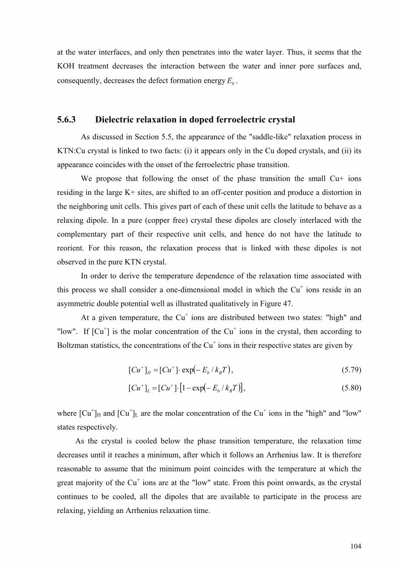
at the water interfaces, and only then penetrates into the water layer. Thus, it seems that the
KOH treatment decreases the interaction between the water and inner pore surfaces and,
consequently, decreases the defect formation energy . bE
5.6.3 Dielectric relaxation in doped ferroelectric crystal
As discussed in Section 5.5, the appearance of the "saddle-like" relaxation process in
KTN:Cu crystal is linked to two facts: (i) it appears only in the Cu doped crystals, and (ii) its
appearance coincides with the onset of the ferroelectric phase transition.
We propose that following the onset of the phase transition the small Cu+ ions
residing in the large K+ sites, are shifted to an off-center position and produce a distortion in
the neighboring unit cells. This gives part of each of these unit cells the latitude to behave as a
relaxing dipole. In a pure (copper free) crystal these dipoles are closely interlaced with the
complementary part of their respective unit cells, and hence do not have the latitude to
reorient. For this reason, the relaxation process that is linked with these dipoles is not
observed in the pure KTN crystal.
In order to derive the temperature dependence of the relaxation time associated with
this process we shall consider a one-dimensional model in which the Cu+ ions reside in an
asymmetric double potential well as illustrated qualitatively in Figure 47.
At a given temperature, the Cu+ ions are distributed between two states: "high" and
"low". If [Cu+] is the molar concentration of the Cu+ ions in the crystal, then according to
Boltzman statistics, the concentrations of the Cu+ ions in their respective states are given by
( )TkECuCu BbH /exp][][ −⋅= ++ , (5.79)
( )[ ]ECuCu bL /exp1][][ −−⋅= ++ TkB , (5.80)
where [Cu+]H and [Cu+]L are the molar concentration of the Cu+ ions in the "high" and "low"
states respectively.
As the crystal is cooled below the phase transition temperature, the relaxation time
decreases until it reaches a minimum, after which it follows an Arrhenius law. It is therefore
reasonable to assume that the minimum point coincides with the temperature at which the
great majority of the Cu+ ions are at the "low" state. From this point onwards, as the crystal
continues to be cooled, all the dipoles that are available to participate in the process are
relaxing, yielding an Arrhenius relaxation time.
104
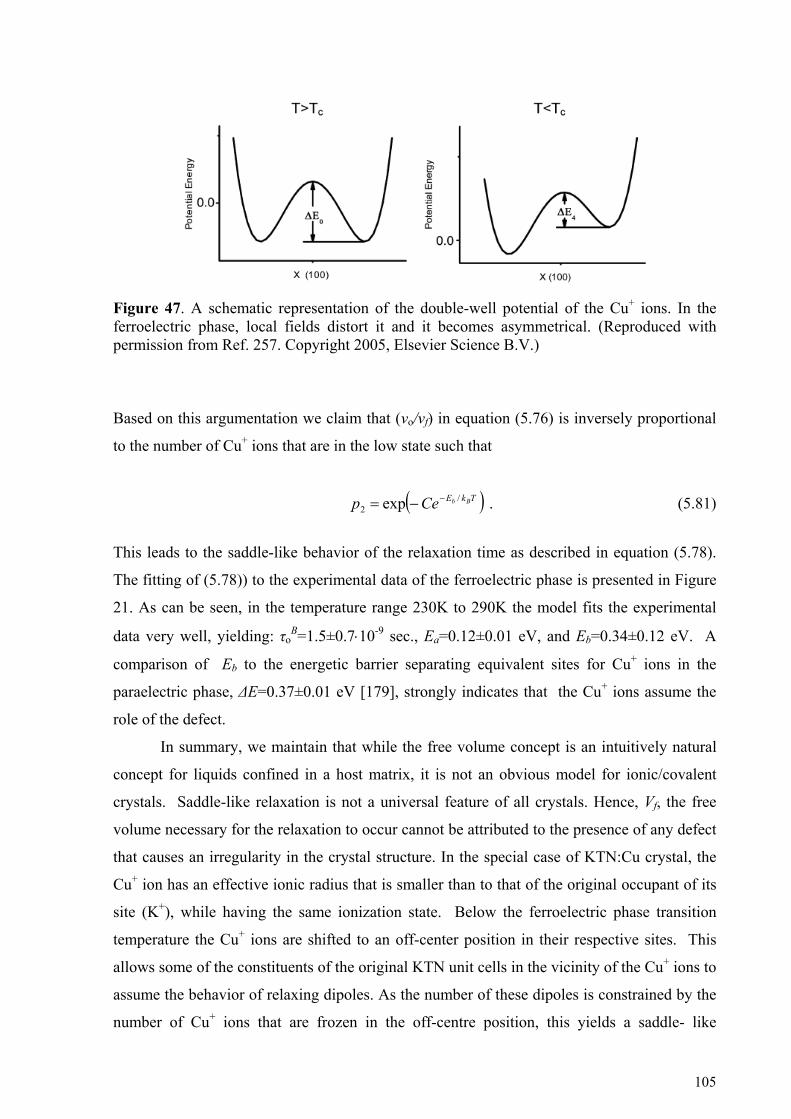
Figure 47. A schematic representation of the double-well potential of the Cu+ ions. In the ferroelectric phase, local fields distort it and it becomes asymmetrical. (Reproduced with permission from Ref. 257. Copyright 2005, Elsevier Science B.V.)
Based on this argumentation we claim that (vo/vf) in equation (5.76) is inversely proportional
to the number of Cu+ ions that are in the low state such that
( )TkE BbCep /2 exp −−= . (5.81)
This leads to the saddle-like behavior of the relaxation time as described in equation (5.78).
The fitting of (5.78)) to the experimental data of the ferroelectric phase is presented in Figure
21. As can be seen, in the temperature range 230K to 290K the model fits the experimental
data very well, yielding: τoB=1.5±0.7⋅10-9 sec., Ea=0.12±0.01 eV, and Eb=0.34±0.12 eV. A
comparison of Eb to the energetic barrier separating equivalent sites for Cu+ ions in the
paraelectric phase, ΔE=0.37±0.01 eV [179], strongly indicates that the Cu+ ions assume the
role of the defect.
In summary, we maintain that while the free volume concept is an intuitively natural
concept for liquids confined in a host matrix, it is not an obvious model for ionic/covalent
crystals. Saddle-like relaxation is not a universal feature of all crystals. Hence, Vf, the free
volume necessary for the relaxation to occur cannot be attributed to the presence of any defect
that causes an irregularity in the crystal structure. In the special case of KTN:Cu crystal, the
Cu+ ion has an effective ionic radius that is smaller than to that of the original occupant of its
site (K+), while having the same ionization state. Below the ferroelectric phase transition
temperature the Cu+ ions are shifted to an off-center position in their respective sites. This
allows some of the constituents of the original KTN unit cells in the vicinity of the Cu+ ions to
assume the behavior of relaxing dipoles. As the number of these dipoles is constrained by the
number of Cu+ ions that are frozen in the off-centre position, this yields a saddle- like
105
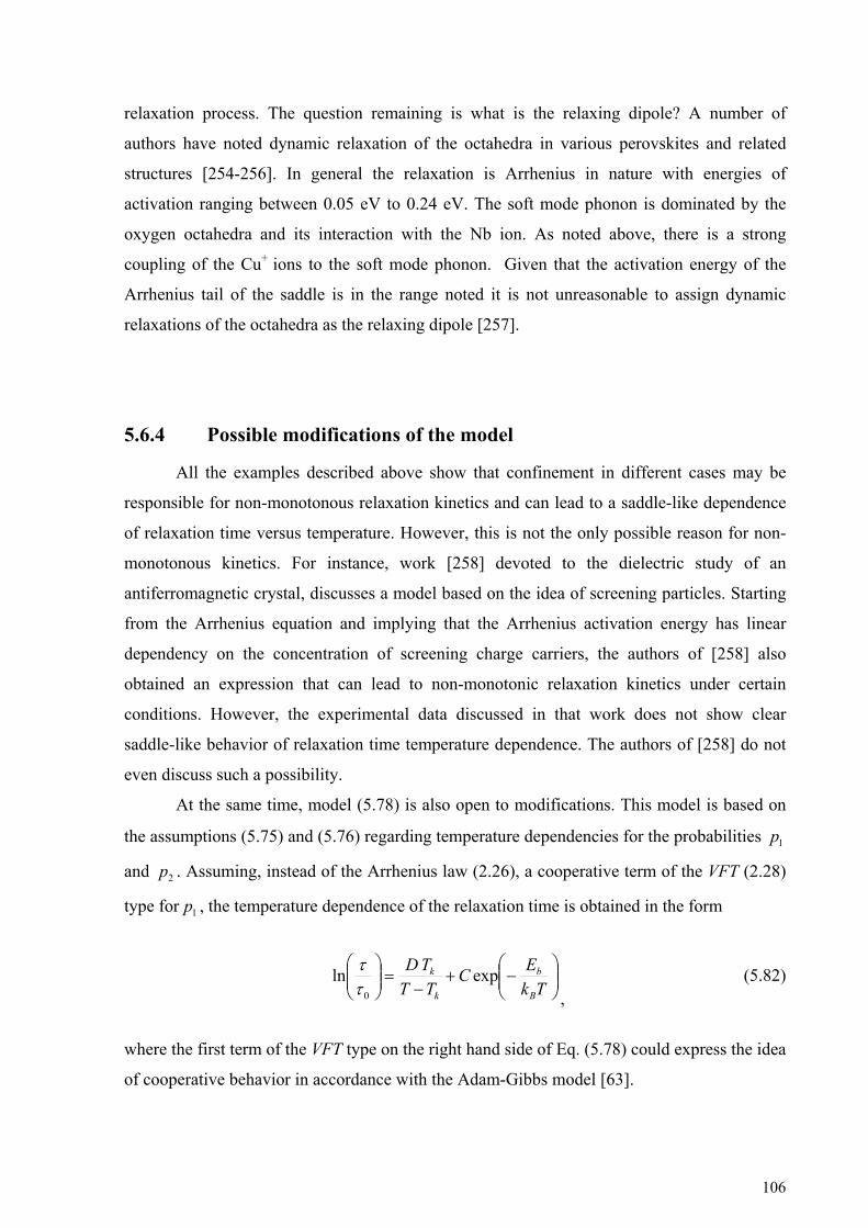
relaxation process. The question remaining is what is the relaxing dipole? A number of
authors have noted dynamic relaxation of the octahedra in various perovskites and related
structures [254-256]. In general the relaxation is Arrhenius in nature with energies of
activation ranging between 0.05 eV to 0.24 eV. The soft mode phonon is dominated by the
oxygen octahedra and its interaction with the Nb ion. As noted above, there is a strong
coupling of the Cu+ ions to the soft mode phonon. Given that the activation energy of the
Arrhenius tail of the saddle is in the range noted it is not unreasonable to assign dynamic
relaxations of the octahedra as the relaxing dipole [257].
5.6.4 Possible modifications of the model
All the examples described above show that confinement in different cases may be
responsible for non-monotonous relaxation kinetics and can lead to a saddle-like dependence
of relaxation time versus temperature. However, this is not the only possible reason for non-
monotonous kinetics. For instance, work [258] devoted to the dielectric study of an
antiferromagnetic crystal, discusses a model based on the idea of screening particles. Starting
from the Arrhenius equation and implying that the Arrhenius activation energy has linear
dependency on the concentration of screening charge carriers, the authors of [258] also
obtained an expression that can lead to non-monotonic relaxation kinetics under certain
conditions. However, the experimental data discussed in that work does not show clear
saddle-like behavior of relaxation time temperature dependence. The authors of [258] do not
even discuss such a possibility.
At the same time, model (5.78) is also open to modifications. This model is based on
the assumptions (5.75) and (5.76) regarding temperature dependencies for the probabilities
and . Assuming, instead of the Arrhenius law (2.26), a cooperative term of the VFT (2.28)
type for , the temperature dependence of the relaxation time is obtained in the form
1p
2p
1p
⎟⎟⎠
⎞⎜⎜⎝
⎛−+
−=⎟⎟
⎠
⎞⎜⎜⎝
⎛Tk
ECTT
TDB
b
k
k exp ln0τ
τ
, (5.82)
where the first term of the VFT type on the right hand side of Eq. (5.78) could express the idea
of cooperative behavior in accordance with the Adam-Gibbs model [63].
106

5.6.4.1 Confined glassy water
The experimental data for water confined in the porous glass sample C that was
discussed previously (see Figure 46) is well fitted with (5.82) as presented in Figure 48.
Figure 48. Temperature dependence of dielectric relaxation time for water confined in sample C. The data were measured under different conditions and contain a different amount of water: Unfilled circles correspond to the data presented early in Fig. 46; filled circles represent the experiment with reduced water content [78]. Full line is the best fit according to (133): 5.08.17ln 0 ±−=τ , kJ/mol 139 ±=bE , K 7124 ±=kT , 210 ±=D
0
, . The dashed line was simulated from (133) for the same
55 103109 ×±×=Clnτ , , and , but with C
divided by a factor 1.8 (explanation in the text). (Reproduced with permission from Ref. 78. Copyright 2004, The American Physical Society.)
bE kT D
Compared to the other samples, this porous glass has the largest pore diameter and humidity
[153,156]. Therefore, it is reasonable to assume that the cooperative relaxation properties,
described by the VFT term, should be more pronounced for this sample. It is worth noting that
the fitted value of the Kauzmann temperature K 7124 ±=kT
kT
(see caption for Figure 48).
From , using the empirical rule TkT g 2.11.1~ ÷ [14], the estimation of the
water glass transition temperature could be obtained. This value is in fair agreement with
usual estimations of for water that are expressed by interval
K 145~gT
K 6gT 130 ±≈gT [259,260]. The
fitted value of fragility is close to the estimations of this parameter 210 ±=D 8≈D that
have been derived from the diffusivity data for the amorphous solid water in work [260].
These findings may also support the idea that the porous glass samples treated in the
preceding discussion dealt with a kind of non-crystalline state of water. The most probable
reason for this is that the pore walls provide the necessary confinement. Note that in the
107

porous glasses, the glassy properties of water can be observed at comparatively high
temperatures such as room temperature, whereas the usually quite low temperatures and
special treatment [259,260] are required to obtain glassy water. However, further
investigations are required to support these experimental findings.
5.6.5 Relationships between the static properties and dynamics
Let us now consider the relationship between the data obtained from the kinetics to the
amplitude of this process. The data for water confined in porous Glass C can be discussed in
terms of equilibrium properties of the considered relaxation processes obtained in the two
different experiments [78]. The two experimental runs presented in Figure 49 are quite similar
at low temperatures. However, in the high temperature range, they exhibit a remarkable
difference from each other.
In Figure 49, the temperature dependencies of the so-called dielectric strength εΔ for
these experiments are presented. The dielectric strength is the difference between the high and
low frequency limits of the real part of the complex dielectric permittivity of the process
under consideration. This quantity reflects the concentration of dipole moments in a
sample and, in its simplest approximation, is in linear proportion to the concentration
dn
Figure 49. Temperature dependence of the dielectric strength εΔ for sample C. Symbols represent experimental data corresponding to the relaxation times presented in Fig. 48: unfilled circles correspond to the data presented early in Fig. 46; filled circles represent the experiment with reduced water content [78]. The lines mark values of the averaged dielectric strength avεΔ for these experiments. (Reproduced with permission from Ref. 78. Copyright 2004, The American Physical Society.)
108

dn~εΔ [6,7], i.e. the dielectric strength is proportional to the water content. Thus, the two
experimental runs presented in Figure 49, as well as the data in Figure 48, correspond to the
two different amounts of water in sample C.
Recall that the pre-exponential factor VnvC /00= , where is the maximum possible
number of defects. This number is proportional to the water content and
0n
εΔ~~~ 0 dnnC .
The dielectric strength εΔ for these runs is almost constant (the variations of εΔ are about
5% of the averaged value for both runs). By comparing the averaged values of εΔ for these
runs the difference in water content between these experiments has been estimated to be 1.8
times (see Figure 49). The pre-exponential factors C for these two runs should also be
different by the same factor. The comparison in Figure 48 shows that this is indeed so.
Finally we can conclude that confinement could be responsible for the non-monotonic
relaxation kinetics and could provide a specific saddle-like temperature dependency of
relaxation time. The experimental examples discussed show that this type of kinetics may be
inherent to systems of completely different natures: confined liquids, ferroelectric crystals,
and it was even demonstrated recently macromolecular folding kinetics [78]. In each case, the
specific interpretation of the parameters of model (5.78) depends on the discussed
experimental situation. We are far from the opinion that confinement is the only reason for
non-monotonic relaxation kinetics. However, for all the examples discussed in this paper, the
non-monotonic dependence of the relaxation time on temperature has the same origin, that is,
confinement either in real or configurational space.
5.7 Dielectric Spectrum Broadening in disordered materials
In the previous sections, we presented several examples of the non-exponential dielectric
response in time domain. We also discussed the dielectric response in H-bonding networks
and liquid like behavior in doped ferroelectric crystals. The models we presented in time
domain enable us to determine some of the topological properties of the investigated complex
systems. We also observed that frequency representation has its own advantages. In particular,
the non-dissipative part of the system response to an external perturbation and the dissipative
part are clearly separated in frequency domain as the real and imaginary part of the complex
permittivity, while in time domain these effects are "mixed" together in the relaxation
function. The separation of the response itself and the dissipative effects in time domain is not
obvious, although it is possible to do in principle by using the appropriate integral transform.
109

In spite of the existence of a single mapping between the time and frequency domain by the
Laplace transform, the separation in frequency representation may at times be more
convenient for analysis of the dynamic processes in complex systems.
In Section 2.2 we classified several types of non-Debye relaxation and mentioned a few
particular approaches which were developed in order to explain the origins of these relaxation
patterns. Below we will discuss a model that considers one particular case of such non-
exponential relaxation.
5.7.1 Symmetric Relaxation peak broadening in complex systems
As mentioned in Section 2.2, the dielectric response in frequency domain for most
complex systems cannot be described by a simple Debye expression (2.17) with a single
dielectric relaxation time. In a most general way this dielectric behavior can be described by
the phenomenological Havriliak-Negami (HN) formula (2.21).
Usually, the exponents α and β are referred to as measures of symmetrical and
unsymmetrical relaxation peak broadening. These names are a consequence of the fact that
the imaginary part of the complex susceptibility for the HN dielectric permittivity shows
power-law asymptotic forms Im{ε*(ω)} ~ ωα and in the low- and high-
frequency limits, respectively.
αβωωε −~)}(*{Im
The experimental data shows that α and β are strictly dependent on temperature, structure,
composition, pressure and other controlled physical parameters [87,261-265].
In this section we will consider the specific case of the HN formula β = 1, 0 < α < 1,
corresponding to symmetric relaxation peak broadening or to the so-called Cole-Cole (CC)
law [16]. The complex dielectric permittivity ε*(ω) for the CC process is represented in the
frequency domain as
αωτεε
εωε)(1
)(*i
i s+
−+= ∞
∞ . (5.83)
In order to explain the non-Debye response (5.83) it is possible to use the memory function
approach [22, 23, 31, 266-268]. Thus, the normalized dipole correlation function Ψ(t) (2.22)
corresponding to a non-exponential dielectric relaxation process obeys the equation
∫ ′′Ψ′−−=Ψ t
tdtttmdt
td
0 )()()( , (5.84)
110

where m(t) is the memory function, and t is the time variable. The specific form of the
memory function is dependent on the features of relaxation.
After Laplace transform (2.15), in virtue of the convolution form, Eq. (5.84) reads as
)()( 1)( pFpMppF −=− , (5.85)
where F(p) and M(p) are Laplace images of Ψ(t) and m(t). Combining (5.85) with (5.83) and
taking into account the relationship between the complex susceptibility and the correlation
function, (2.14), one can obtain the Laplace image of the memory function for the CC process
in the form αατ −−= 1)( ppM . (5.86)
Since 0 < α < 1 the exponent in Eq.(5.86) 1-α > 0. The mathematical implication is that M(p)
(5.86) is a multi-sheet function of complex variable p. In order to represent this function in the
time domain one should to select the Schlicht domain using supplementary physical
explanations [135]. These computational constraints can be avoided by using the Riemann-
Liouville fractional differential operator α−10 tD
)]([ tΨ
(see definitions (5.46) (5.47)). Thus, one can
easily see that the Laplace image of 10 Dt
−α is
.)]([
where
)()]]([[ˆ
00
110
+=−
−−
Ψ=
−=Ψ
t
t
tDC
CpFptDL
α
αα
(5.87)
Taking (5.87) into account we can rewrite Eq. (5.84) with the memory function (5.86) as
follows
)]([)( 10 tD
dttd
t Ψ−=Ψ −− αατ . (5.88)
Note that the relationship between the complex susceptibility and correlation function
(2.14), together with Eq. (5.83) leads directly to the requirement that C=0.
Equation (5.88) was already discussed elsewhere [22, 23, 31] as a phenomenological
representation of the dynamic equation for the CC law. Thus, Eq. (5.88) shows that since the
fractional differentiation and integration operators have a convolution form it can be regarded
111
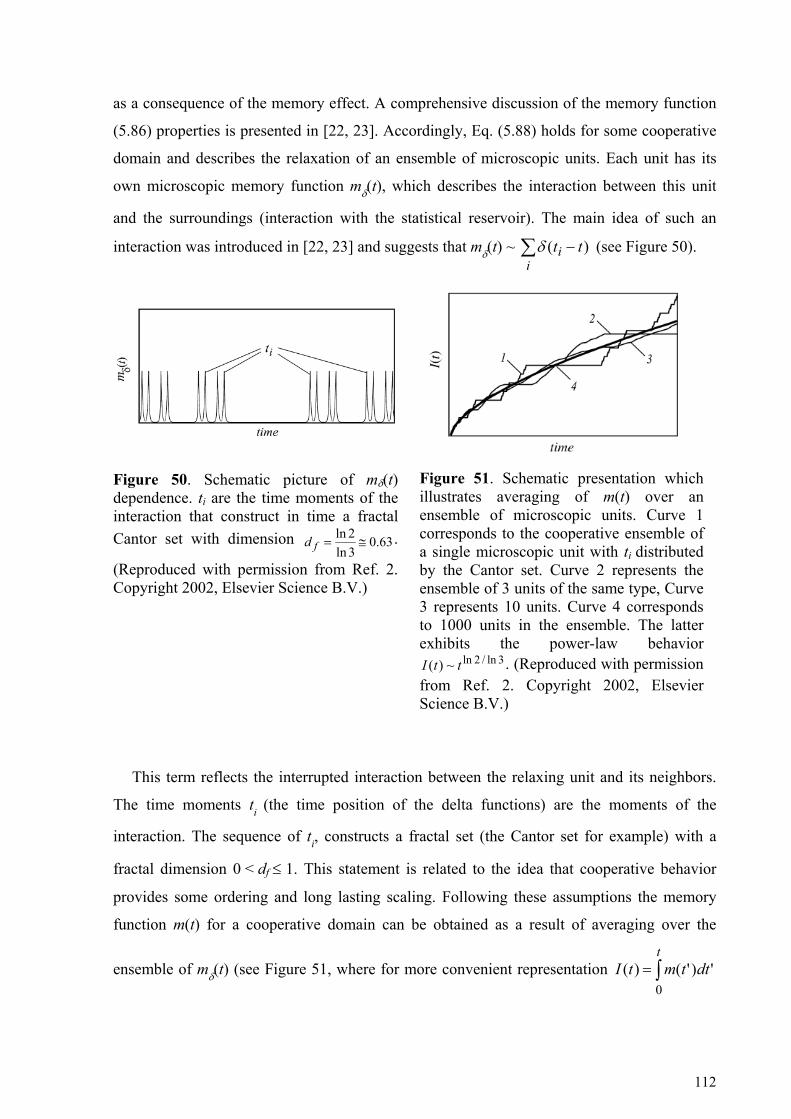
as a consequence of the memory effect. A comprehensive discussion of the memory function
(5.86) properties is presented in [22, 23]. Accordingly, Eq. (5.88) holds for some cooperative
domain and describes the relaxation of an ensemble of microscopic units. Each unit has its
own microscopic memory function mδ(t), which describes the interaction between this unit
and the surroundings (interaction with the statistical reservoir). The main idea of such an
interaction was introduced in [22, 23] and suggests that mδ(t) ~ ∑ −i
i tt )(δ (see Figure 50).
Figure 50. Schematic picture of mδ(t) dependence. ti are the time moments of the interaction that construct in time a fractal Cantor set with dimension 63.0
3ln2ln
≅=fd .
(Reproduced with permission from Ref. 2. Copyright 2002, Elsevier Science B.V.)
Figure 51. Schematic presentation which illustrates averaging of m(t) over an ensemble of microscopic units. Curve 1 corresponds to the cooperative ensemble of a single microscopic unit with ti distributed by the Cantor set. Curve 2 represents the ensemble of 3 units of the same type, Curve 3 represents 10 units. Curve 4 corresponds to 1000 units in the ensemble. The latter exhibits the power-law behavior
. (Reproduced with permission from Ref. 2. Copyright 2002, Elsevier Science B.V.)
3ln/2ln~)( ttI
This term reflects the interrupted interaction between the relaxing unit and its neighbors.
The time moments ti (the time position of the delta functions) are the moments of the
interaction. The sequence of ti, constructs a fractal set (the Cantor set for example) with a
fractal dimension 0 < df ≤ 1. This statement is related to the idea that cooperative behavior
provides some ordering and long lasting scaling. Following these assumptions the memory
function m(t) for a cooperative domain can be obtained as a result of averaging over the
ensemble of mδ(t) (see Figure 51, where for more convenient representation ∫=t
dttmtI0
')'()(
112

is plotted instead of m(t)). The requirements of measure conservation in the interval [0, 1/ζ]
and conservation of the fractal dimension df for all mδ(t) give this averaging as
. ~)(
and
)()(
1
2/1
2/1
)1(
f
f
d
-duu
ppM
dutmtm
−
−
−−∫= ζζδ
(5.89)
Thus, the memory function (5.86) is a cooperative one and the CC behavior appears on the
macroscopic level after averaging over the ensemble of microscopic dipole active units.
Comparing (5.86) and (5.89) one can establish that fd=α . This result once again highlights
the fact that in this model the fractal properties on a microscopic level induce the power-law
behavior of memory functions (5.86), (5.89) and CC permittivity (5.83) on a macroscopic
level.
By definition [213, 220], the fractional dimension is given by
)ln()ln(
ζα Nd f == . (5.90)
Here the scaling parameter ζ is the dimensionless time interval size and N is the number of
delta functions (relaxation acts) in that interval. However, a characteristic time constant of the
CC process is the relaxation timeτ. Thus, the scaling parameter ζ and the relaxation time
should be proportional to each other
0ττζ = . (5.91)
The constant minimal τ0 is the cutoff time of the scaling in time.
In the general case, different physical conditions can determine the fractal properties of the
microscopic memory function mδ(t) and, consequently, the power-law time dependence of the
macroscopic memory function (5.89). However, there is a computer simulation proof [269]
that an anomalous relaxation on a fractal structure exhibits CC behavior. Therefore, one may
assume that the memory function (5.89) has its origin in the geometrical self-similarity of the
investigated system. Thus, the scaling parameter N is actually the number of points where the
relaxing units are interacting with the statistical reservoir (i.e. by the ergodic assumption - the
113

number of relaxation acts on a microscopic level for a cooperative domain). The assumption
of geometrical self-similarity of the considered system suggests that this number is
Gd
RRGN ⎟⎟
⎠
⎞⎜⎜⎝
⎛=
0 . (5.92)
Here, dG is a spatial fractal dimension of the point set where relaxing units are interacting with
the surroundings. R is the size of a sample volume section where movement of one relaxing
unit occurs. R0 is the cutoff size of the scaling in the space or the size of the cooperative
domain. G is a geometrical coefficient about unity, which depends on the shape of the system
heterogeneity. For example, the well-known two-dimensional recurrent fractal Sierpinski
carpet has 1.89, ≈= )3ln(/)8ln(Gd ≈= 4/3G 0.43 [213].
The relaxation process may be accompanied by a diffusion act. Consequently, the mean
relaxation time for such kinds of disordered systems is the time during which the relaxing
microscopic structural unit would move a distance R. The Einstein-Smoluchowski theory
[226,235] gives the relationship between τ and R as
τDdR E22 = , (5.93)
where D is the diffusion coefficient and dE is the Euclidean dimension. Thus, combining the
relationships (5.90)-(5.93) one can obtain the relationship between the Cole-Cole parameter α
and the mean relaxation time τ in the form
)/ln()ln(
2 0τττω
α sGd= , (5.94)
where 20
22RDGd Gd/
Es =ω is the characteristic frequency of the diffusion process. This
equation establishes the relationship between the CC exponent α, the relaxation time τ, the
geometrical properties (fractal dimension dG), and the diffusion coefficient (through ωs).
114

5.7.2 Polymer-water mixtures
The first mention of the α(τ) dependencies was in the experimental work [265]. The
dielectric relaxation data of water in the mixtures of seven water-soluble polymers was
presented there. It was found that in all these solutions relaxation of water obeys the CC law,
while the bulk water exhibits the well-known Debye-like pattern [270,271]. Another
observation was that α is dependent not only on the concentration of solute but also on the
hydrophilic (or hydrophobic) properties of the polymer. The seven polymers were:
poly(vinylpyrrolidone) (PVP; weight average molecular weight (Mw) = 10,000),
poly(ethylene glycol) (PEG; Mw = 8,000), poly(ethylene imine) (PEI; Mw = 500,000),
poly(acrylic acid) (PAA; Mw = 5,000), poly(vinyl methyl ether) (PVME; Mw = 90,000),
poly(allylamine) (PAlA; Mw = 10,000), and poly(vinyl alcohol) (PVA; Mw = 77,000). These
polymers were mixed with different ratios (up to 50% of polymer in solution) to water and
measured at a constant room temperature (25°C ) [265].
We would like to sketch a recent application [46] of model (5.94) to these systems. In
Figure 52 the experimental dependencies of CC exponent α versus τ together with the fitting
curve are presented. The values of the fitting parameters are listed in Table 3.
Table 3. The space fractional dimension dG, the cutoff time of the scaling in the time domain τ0, the characteristic frequency sω and estimated self-diffusion coefficient for the polymer water mixturesb.
Sample dG τ0 [ps] ω s × 10-11 [Hz] D× 109 [m2s-1]
PVA 1.56±0.09 7.18±0.74 1.47±0.21 3.31
PAlAb 1.43 6.46 1.74 3.92
PAA 1.12±0.17 6.34±0.83 2.08±0.68 4.68
PEI 1.33±0.02 4.89±0.45 2.67±0.40 6.01
PEG 1.54±0.04 4.45±0.74 2.78±0.63 6.26
PVME 1.38±0.10 3.58±1.23 4.24±2.47 9.54
PVP 1.00±0.01 0.79±0.11 127±34 286
bFor the sample PAlA there are only three experimental points. For this reason it is impossible to determine the mean square deviation value and consequently the confidence intervals for the fitting parameters. Source: (Reproduced with permission from Ref. 46. Copyright 2002, American Institute of Physics.
115

It is well known [54,270] that the macroscopic dielectric relaxation time of bulk water (8.27ps
at 25°C) is about ten times greater than the microscopic relaxation time of a single water
molecule, which is about one hydrogen bond lifetime [206,272-274] (about 0.7 ps). This fact
follows from the associative structure of bulk water where the macroscopic relaxation time
reflects the cooperative relaxation process in some cluster of water molecules.
In the framework of the model presented above the microscopic relaxation time of
water molecule is equal to the cut off time of the scaling in time domain τ0.
Figure 52. Cole–Cole exponent α versus relaxation time τ for PVA (●), PAlA (▲), PAA (■), PEI (♦), PEG (○), PVME ( Δ ), and PVP (□) samples. The curves correspond to the model described in this section. The filled symbols correspond to the hydrophilic polymers and the open symbols correspond to the hydrophobic samples. (Reproduced with permission from Ref. 2. Copyright 2002, Elsevier Science B.V.)
For the most hydrophilic polymer, PVA, the strong interaction between the polymer and the
water molecule results in the greatest value of microscopic relaxation time τ0 , only 10% less
than the macroscopic relaxation time of the bulk water. The most hydrophobic polymer, PVP,
has the smallest value of a single water molecule microscopic relaxation time, which is almost
equal to the microscopic relaxation time of bulk water (see Table 3). Therefore, weakening
the hydrophilic properties (or intensifying the hydrophobic properties) results in a decreasing
of interaction between the water and the polymer and consequently in the decrease of τ0.
The interaction between the water and the polymer occurs in the vicinity of the polymer
chains and only the water molecules situated in this interface are affected by the interaction.
The space fractal dimension dG in this case is the dimension of the macromolecule chain. If a
polymer chain is stretched as a line, then its dimension is 1. In any other conformation, the
116

wrinkled polymer chain has a larger space fractal dimension, which falls into the interval
1 < dG < 2. Thus, it is possible to argue that the value of the fractal dimension is a measure of
polymer chain meandering. Straighter (probably more rigid) polymer chains have dG values
close to 1. More wrinkled polymer (probably more flexible) chains have dG values close to 2
(see Table 3).
The presence of a polymer in the water affects not only the relaxation but the diffusion of
the solvent as well. For an estimation of the diffusion coefficient, we can use the following
expression
E
sdR
D2
20ω
≅ , (5.95)
which is directly derived from the definition of the characteristic frequency ωs. It was
assumed in this last expression that the geometrical factor G=1. In our case the scaling cut-off
size in space is equal to the diameter of a water molecule ≈0R 3 Å [52]. The Euclidean
dimension of the space where diffusion occurs is the nearest integer number greater than the
fractal dimension. Thus, dE = 2. The results of this estimation are in Table 3. The diffusion
coefficient for bulk water [52] at 25°C is 2.57⋅10-9 m2s-1. The presence of a polymer in the
water prevents clusterization of water and relieves the diffusion. However, the strong
interaction between polymer and water for hydrophilic samples slows down the diffusion. The
competition between these two effects leads to the clear tendency of the diffusion coefficient
to increase with an increase of hydrophility (see Table 3).
Note that the polymer affects only water molecules situated in the vicinity of the polymer
chains. Thus, the estimated diffusion coefficient corresponds only to these water molecules
and is not dependent on the polymer concentration. The averaged self-diffusion coefficient
estimated for the entire polymer-water mixture should be different depending on the polymer
concentration.
117
5.7.3 Micro-composite material
Another example of an application of Eq. (5.94) is on micro-composite polymer materials.
We have performed dielectric measurements of the glass transition relaxation process in a
Nylon 6,6 sample quenched in amorphous (QN), a crystalline nylon 6,6 sample (CN) and a
micro-composite sample (MCN), which is the same crystalline nylon 6,6 but with
incorporated kevlar fibers [275,276].
The quantitative analysis of the dielectric spectra of the glass-transition process was carried
out by fitting the isothermal dielectric loss data according to the HN law (2.21). It was found
from the fitting that β=1 for the glass-transition process in all of the samples measured. The
glass-transition relaxation process in these systems is due to the motion of a polymer chain
that is accompanied by a diffusion act. In general, the diffusion of a polymer chain is more
complex than the Brownian model for diffusion [277,278]. However, in all the models the
dependence of <R2> on time t is linear in the time scales associated with a monomeric link
and in the time scale associated with the mobility of the entire chain. For this particular
example, Eq. (5.93) describes the mobility of the polymer groups at the microscopic levels,
i.e. at the scale of a monomeric link.
The experimental α versus τ dependencies for these samples, together with the fitting
curves, are shown in Figure 53. Note that in contrast with the previous example these data are
obtained at a constant sample composition. In this case, variations of parameters α and τ are
induced by temperature variation. As mentioned above, the exponents α as well as the
relaxation time τ are the functions of the different experimentally controlled parameters. The
same parameters can affect the structure or the diffusion simultaneously. In particular, both α
and τ are functions of temperature.
Thus, the temperature dependence of the diffusion coefficient in (5.93) should be
considered. Let us consider the temperature dependence of the diffusion coefficient D
)T(KDD 0= , (5.96)
where K(T) is a dimensionless function that represents the temperature dependence of the
diffusion coefficient. D0 is the appropriate constant with dimensions [m2s-1]. An increase of
the diffusion
118

Figure 53. The dependence of α versus relaxation time τ for QN (●), CN (▲), and MCN (♦) samples. The curves correspond to the model described in this section. (Reproduced with permission from Ref. 2. Copyright 2002, Elsevier Science B.V.)
coefficient with increasing temperature also signifies an increase of the characteristic spatial
scale R0 (cut-off size of the scaling in the space). Let us assume that is proportional to the
diffusion coefficient D and obeys the Einstein Smoluchowski theory
20R
maxE τDdR 220 = , (5.97)
where τmax is the long-time limit of the scaling. Thus, combining together (5.96) and (5.97)
with (5.91)-(5.93) we can obtain the relationship between the CC exponent α and relaxation
time τ in a form similar to (5.94)
)/ln()ln(
2 0
0ττ
τωα Gd
= , (5.98)
with substitution of ωs by max
d/ GGτ
ω2
0 = . The latter relationship shows that under assumption
(5.97) the temperature dependence of the diffusion coefficient does not change the form of the
α versus τ relationship.
The average length of a nylon 6,6 polymer chain is about 50-100 μm (each polymer chain
contains about 105 groups while the length of a polymer group rg is about 10 Å). This length
is comparable to the thickness of a sample 120-140 μm [275]. Thus, the movement of the
chains is most likely occurring in the plane of the sample. This fact correlates with the values
119

of the space fractional dimension dG. For all of the samples dG ∈ (1, 2) (see Table 4). Thereby,
the Euclidean dimension of the space in which chain movement occurs is dE = 2.
Table 4. The space fractional dimension dG, the cutoff time of the scaling in the time domain τ0 and the characteristic frequency 0ω for quenched polymer (QN), crystalline (CN) and micro-composite samples (MCN). Source: Reproduced with permission from Ref. 2. Copyright 2002, Sage Publications.
Sample dG τ0 [ms] ω 0 [kHz]
QN 1.12±0.01 1.1±0.1 5.9±0.3
CN 1.20±0.05 5.8±4.4 9.7±1.9
MCN 1.04±0.02 1.5±0.4 8.1±0.7
Although there is no unambiguous data for the mesoscale structure of the samples under
investigation at this time, nevertheless it is possible to estimate the order of magnitude of
some physically significant quantities from the cutoff time τ0 and characteristic frequency ω0
values. Despite the fact that ω0 and ωs have different physical significance, for the estimation
one can neglect the temperature dependence of the diffusion coefficient and assume that
10-16 m2 ( is the cube root of the volume occupied by one polymer chain), ≈20R 0R ≈G 1.
Then, the self-diffusion coefficient evaluated by expression (5.15) falls into the interval 10-14
to 10-13 m2s-1, which is typical for such polymer materials [279-281].
The cutoff time τ0 is related to the size of the cooperative domain lc by . Thus,
in the two-dimensional case one can estimate the number of polymer groups, ng in the
cooperative region as 102, which is in fair agreement with the results obtained
in the paper [282].
02 4 τ Dlc =
≈= 22 / gcg rln
One can also see from Table 4 that the presence of either the crystalline phase or the kevlar
fibers in a sample leads to an increase of the cutoff time τ0, indicating a slowdown of the
relaxation process. Their presence also leads to an increase of the ω0 value as well. This is a
manifestation of a decreasing mobile polymer chain length.
Concluding this section we can summarize as follows: the model of symmetric relaxation
peak broadening presented here is not universal. However, it was illustrated through two
examples that this model can describe some common features of relaxations of this type.
Thought, not a universal model, it, nevertheless, provides the relationship between
120
microscopic parameters of experimental samples and properties of experimentally measured
macroscopic correlation functions. Thus, we hope that it may be useful in other cases where a
dielectric relaxation of the Cole-Cole type is present.
121
6 Summary In conclusion, we would like to recapitulate the main goals of this tutorial. We
demonstrated the effectiveness of dielectric spectroscopy as a tool for investigating complex
materials. The unique capabilities of DS allowed us to investigate materials in a broad time
scale range, to identify general relaxation phenomena and to discover new ones for the studied
complex systems, independent of the particularity of the material. DS makes it possible to
cover extremely wide continuous ranges of experimentally controlled parameters, a feature
that no other existing spectroscopic method today can offer. Moreover, this method, once
again as compared to the conventional radio spectroscopic techniques such as electron
paramagnetic or nuclear magnetic resonance, is much simpler in terms of hardware
realization. We also presented current state-of-the-art applications of DS including the
resolution of some of the critical issues related to hardware and modern data treatment
procedures, which make possible the recent achievements of this method. Last, but not least,
in this tutorial we discussed some contemporary ideas that are currently employed by the
dielectric community. In this regard the DS studies of different complex materials presented
in this tutorial demonstrate the capability to generate new knowledge about the cooperative
dynamics in quite different complex structures [283-286]. It was shown that despite the
morphological differences of the systems studied, the most general feature of the relaxation
processes observed by DS is the Non-Debye Dielectric Response, which is a consequence of
the cooperative dynamics and confinement that also lead to Non-Arrhenius kinetics.
7 Acknowledgements We would like to thank Alexander Puzenko, Anna Greenbaum and Paul Ben Ishai from
Department of Applied Physics, The Hebrew University of Jerusalem, Israel for numerous
discussions and stimulating advice.
122

8 References 1. M.F. Shlesinger, G.M. Zaslavsky, and J. Klafter, Nature 363, 31 (1993).
2. Yu. Feldman, A. Puzenko and Ya. Ryabov, Chem. Phys. 284, 139 (2002).
3. F. Kremer and A. Schönhals, eds., Broadband Dielectric Spectroscopy, Springer-
Verlag, Berlin, 2003.
4. R.N. Clarke, ed., A Guide to the characterization of dielectric materials of RF and
microwave frequencies, NPL, London, 2004.
5. Yu. Feldman, I. Ermolina, and Y. Hayashi, IEEE Trans. Dielectr. Electr.Insul. 10, 728
(2003).
6. H. Fröhlich, Theory of dielectrics. Dielectric constant and Dielectric Loss second
edition, Clarendon Press, Oxford, 1958.
7. C.J.F. Böttcher, Theory of Electric Polarization, vol. 1, second edition, Elsevier Science
B.V., Amsterdam, 1993.
8. N.E. Hill, W.E. Yaughan, A. H. Price and M. Davis, Dielectric Properties and
Molecular Behavior, Van Nostrand, London, 1969.
9. N. Kozlovich, A. Pusenko, Yu. Alexanadrov, and Yu. Feldman, Colloids and Surfaces
A. 140, 229 (1998).
10. A. Volmari and H. Weingärtner, J. Mol. Liq. 98–99, 293 (2002).
11. J.F. Böttcher and P. Bordewijk, Theory of Electric Polarisation, vol. 2, second edition,
Elsevier Science B.V., Amsterdam, 1992.
12. B.K.P. Scaife, Principles of Dielectrics, Oxford University press, Oxford, 1989.
13. A.N. Tikhonov and V.Y. Arsenin, Solutions of Ill-Posed Problems, J. Wiley, New
York, 1977.
14. H. Schäfer, E. Sternin, R. Stannarius, M. Arndt and F. Kremer, Phys. Rev. Let. 76,
2177 (1996).
15. S. Havriliak and S. Negami, J. Pol. Sci.: Part C 14, 99 (1966).
16. K.S. Cole and R.H. Cole, J. Chem. Phys. 9, 341 (1941).
17. D.W. Davidson and R.H. Cole, J. Chem. Phys. 19, 1484 (1951).
18. A.K. Jonscher, Dielectric Relaxation in Solids, Chelsea Dielectric press, London,
1983.
19. A.K. Jonscher, Universal Relaxation Law, Chelsea Dielectric Press, London, 1996.
20. J.C. Dyre and T.B. Schrøder, Rev. Mod. Phys. 72, 873 (2000).
21. N.F. Mott and E.A. Davis, Electronic Processes in Non-Crystalline Materials,
Clarendon Press, Oxford, 1978.
123

22. R.R. Nigmatullin and Ya.E. Ryabov, Phys. Solid State 39, 87 (1997).
23. L. Nivanen, R. Nigmatullin and A. LeMehaute, Le Temps Irreversible a Geometry
Fractale, Hermez, Paris, 1998.
24. S. Alexander, J. Bernasconi, W.R. Schneider and R. Orbach, Rev. Mod. Phys. 53, 175
(1981).
25. M. Ben-Chorin, F. Möller, F. Koch, W. Schirmacher and M. Eberhard, Phys. Rev. B
51, 2199 (1995).
26. W.T. Coffey, J. Mol. Liq. 114, 5 (2004).
27. G. Williams, Chem. Rev. 72, 55 (1972).
28. R.H. Cole, in: Molecular Liquids NATO ASI Ser. C 135, 59 (1984).
29. R. Kohlrausch, Ann. Phys. 12, 393 (1847).
30. G. Williams and D.C. Watts, Trans. Farad. Soc. 66, 80 (1970).
31. R. Metzler and J. Klafter, Phys. Rep. 339, 1(2000).
32. A. Blumen, J. Klafter and G. Zumofen, in: I. Zschokke (Ed.) Optical Spectroscopy of
Glasses, Reidel, Dordrecht, Netherlands, p. 199, 1986.
33. G.H. Weiss, Aspects and Applications of the Random Walk, North-Holland,
Amsterdam, 1994.
34. E. Barkai, R. Metzler and J. Klafter, Phys. Rev. E 61, 132 (2000).
35. T. Zavada, N. Südland, R. Kimmich and T.F. Nonnenmacher, Phys. Rev. E 60, 1292
(1999).
36. R. Kimmich, Chem. Phys. 284, 253(2002).
37. T. Wadayama, S. Yamamoto and A. Hatta, Appl. Phys. Lett. 65, 1653 (1994).
38. V. Degiorgio, R. Piazza, F. Mantegazza and T. Bellini, J. Phys.: Condens. Matter 2,
SA69 (1990).
39. J.E. Martin, D. Adolf and J.P. Wilcoxon, Phys. Rev. A 39, 1325 (1989).
40. A. Bello, E. Laredo and M. Grimau, Phys. Rev. B 60, 12764 (1999).
41. F. Alvarez, A. Alegría, J. Colmenero, Phys. Rev. B 44, 7306 (1991).
42. G. Katana, E.W. Fischer, Th. Hack, V. Abetz and F. Kremer, Macromolecules 28,
2714 (1995).
43. R.V. Chamberlin, Phys. Rev. Lett. 82, 2520 (1998).
44. K. Weron and A. Klauzer, Ferroelectrics 236, 59 (2000).
45. Application of Fractional Calculus in Physics, edited by R. Hilfer, World Scientific,
Singapore, 2000.
124

46. Y.E. Ryabov, Y. Feldman, N. Shinyashiki and S. Yagihara J. Chem. Phys. 116, 8610
(2002).
47. Yu. Feldman, N. Kozlovich, Y. Alexandrov, R. Nigmatullin and Y. Ryabov,
Phys. Rev. E. 54 5420 (1996).
48. S. Arrhenius, Z. Physik. Chem. 4, 226 (1889).
49. H. Eyring, Chem. Rev. 17, 65 (1935).
50. H. Eyring, J. Chem. Phys. 3, 107 (1935).
51. H. Eyring, Trans. Faraday. Soc. 34, 41 (1938).
52. D. Eisenberg and W. Kauzmann, The structure and Properties of Water, Clarendon,
Oxford, 1969.
53. J. Barthel, R. Buchner and B. Wurm, J. Mol. Liq. 98-99, 51 (2002).
54. R. Buchner, J. Barthel and J. Stauber, Chem. Phys. Lett. 306, 57 (1999).
55. C.A. Angell, J. Non-Cryst. Solids 73, 1 (1985).
56. C.A. Angell, J. Non-Cryst. Solids 131-133, 13 (1991).
57. R. Böhmer, K.L. Ngai, C. A. Angell and D. J. Plazek, J. Chem. Phys. 99, 4201 (1993).
58. R. Richert and C.A. Angell, J. Chem. Phys. 108, 9016 (1998).
59. R. Brand, P. Lunkenheimer and A. Loidl, J. Chem. Phys. 116, 10386 (2002).
60. H. Vogel, Physik. Z. 22, 645 (1921).
61. G.S Fulcher, J. Am. Ceram. Soc. 8, 339 (1925).
62. G.Tammann and W. Hesse, Z. Anorg. Allg. Chem. 156, 245 (1926).
63. G. Adam and J. H. Gibbs, J. Chem. Phys. 43, 139 (1965).
64. W. Kauzmann, Chem. Rev. 43, 219 (1948).
65. C.A. Angell, Chem. Rev. 102, 2627 (2002).
66. T.G. Fox and P. J. Flory, J. App. Phys. 21, 581 (1950).
67. T.G. Fox and P. J. Flory, J. Phys. Chem. 55, 221 (1951).
68. T.G. Fox and P. J. Flory, J. Pol. Sci. 14, 315 (1954).
69. A.K. Doolittle, J. App. Phys. 22, 1471 (1951).
70. D. Turnbull and M.H. Cohen, J. Chem. Phys. 34, 120 (1961).
71. J.T. Bendler and M.F. Shlesinger, J. Mol. Liquids 36, 37 (1987).
72. J.T. Bendler, M.F. Shlesinger, J. Stat. Phys. 53, 531 (1988).
73. J.T. Bendler, J.J. Fontanella and M.F. Shlesinger, Phys. Rev. Lett. 87, 195503 (2001).
74. W. Götze and L. Sjögren, Rep. Prog. Phys. 55, 241 (1992).
75. U. Bengtzelius, W. Götze and A. Sjölander, J. Phys. C: Solid State Phys. 17, 5915
(1984).
76. P. Taborek and R.N. Kleiman, D.J. Bishop, Phys. Rev. B 34, 1835 (1986).
125

77. R. Richert and H. Bässler, J. Phys.: Condens. Matter 2, 2273 (1990).
78. Y.E. Ryabov, A. Puzenko and Yu. Feldman, Phys. Rev B. 69, 0142041 (2004).
79. R.H. Cole, J.G. Berberian, S. Mashimo, G. Chryssikos, A. Burns and E. Tombari,
J. Appl. Phys. 66, 793 (1989).
80. V.L. Odivanov, Yu.A. Gusev, The journal Pribory i tekhnika eksperimenta, 6, 114
(1986).
81. J.G. Berberian and E. King, J. Non.-Crys. Solids, 305, 10 (2002).
82. S. Mashimo, T. Umehara, T. Ota, S. Kuwabara, N. Shinyashiki and S. Yagihara,
J. Molec. Liq. 36, 135 (1987).
83. D. Bertolini, M. Cassettari, G. Salvetti, E. Tombari and S. Veronesi, Rev. Sci. Instrum.
62, 450 (1991).
84. R. Nozaki and T. K. Bose, IEEE Trans. Instrum. Meas. 39, 945 (1990).
85. B. Gestblom, E. Noreland and J. Sjöblom, J. Phys Chem. 91, 6329 (1987).
86. Yu. Feldman, A. Andrianov, E. Polygalov, I. Ermolina, G. Romanychev, Yu. Zuev
and B. Milgotin, Rev. Sci. Instrum. 67, 3208 (1996).
87. A. Schönhals, F. Kremer and E. Schlosser, Phys. Rev. Lett. 67, 999 (1991).
88. U. Kaatze, V. Lonneckegabel and R. Pottel, Zeitschrift Fur Physikalische Chemie-
International Journal of Research in Phys. 175, 165 (1992).
89. V.L. Odivanov, L.M. Ismagilov, R.M. Shagiev, Yu.A. Gusev, The journal
Phizicheskoi khimii, Vol. LXIII, 2, 568 (1989).
90. F. Kremer, D. Boese, G. Meier, E.W. Fischer, Prog Colloid Polym Sci 80,129 (1989).
91. U. Kaatze and K. Giese J.Phys.E: Sci Instrum 13,133 (1980).
92. R. Böhmer, M. Maglione, P. Lunkenheimer and A. Loidl, J. Appl. Phys. 65, 901
(1989).
93. J.R. Birch, and T.J. Parker, Dispersive Fourier Transform Spectroscopy Chapter 3 in
K.J. Batton (Ed) Infrared and Millimeter Waves Vol. 2: Instrumentation” Academic
Press, NY, pp.137-271, 1979.
94. H.P. Schwan, Determination of biological impedances. In: W.L. Nastuk, editor.
Physical techniques in biological research, vol. VI. New York: Academic Press; p.
323–407. Part B. 1963.
95. K. Asami, Prog. Polym. Sci. 27, 1617 (2002).
96. E.H. Grant, R.J Sheppard and G.P. South Dielectric Behavior of Biological Molecules
in Solution, Oxford: Oxford University Press, chapter 3, 1978.
97. R.E. Collin Foundations for microwave engineering, 2nd dn. McGraw-Hill, NY 1966.
98. F. Kremer J.Non.-Crys.Solids 305, 1 (2002).
126

99. F.I. Mopsic, Rev. Sci. Instrum. 55, 79 (1984).
100. R. Richert, Rev. Sci. Instrum. 67, 3217 (1996)
101. R. Richert, Physica A 287, 26 (2000).
102. R. Richert, J.Non.-Crys.Solids, 305, 29 (2002).
103. Yu.D. Feldman, Yu.F. Zuev, E.A. Polygalov and V.D. Fedotov, Colloid & Polymer
Science 270, 768 (1992).
104. B. Gestblom and P. Gestblom, Macromolecules, 24, 5823 (1991)
105. R.H. Cole, Dielectric Polarization and Relaxation, in: NATO ASI Ser., Ser. C
Vol. 135, “Molecular Liquids”, 1984, p. 59-110.
106. Yu.D. Feldman and V.V. Levin, Chem. Phys. Lett, 85, 528 (1982).
107. A.M. Bottreau and A. Merzouki, IEEE Trans Instrum. Meas. 42, 899 (1993).
108. Time Domain Measurements in Electromagnatics, (E.K. Miller, ed.) Van Nostrand
Reinhold Co, New York, 1986.
109. R. Nozaki and T.K. Bose, IEEE Trans. Instrum. Meas. 39, 945 (1990).
110. N. Miura, N. Shinyashiki, S. Yagihara and M. Shiotsubo, J. Amer. Ceramic. Soc. 81,
213 (1998).
111. R. Buchner and J. Barthel Ber. Bun. Phys. Chem. Chem. Phys. 101, 1509 (1997).
112. N.E. Hager III, Rev. Sci. Instrum. 65, 887 (1994).
113. Yu. Feldman, T. Skodvin and J. Sjöblom, Dielectric Spectroscopy on Emulsion and
Related Colloidal Systems-A Review in Encyclopedic Handbook of Emulsion
Technology, Marcel Dekker, Inc., New York, Basel, (2001), pp.109-168.
114. O. Göttmann, U. Kaatze and P. Petong, Meas. Sci. Tech. 7, 525 (1996).
115. A. Oka, R. Nozaki and Y. Shiozaki, Ferroelectrics 230, 459 (1999).
116. J.G. Berberian and R.H. Cole, Rev. Sci. Instr. 63, 99 (1992).
117. J.P. Grant, R.N. Clarke, G.T. Symm and N.M Spyrou, Phys. Med. Biol. 33, 607
(1988).
118. J.P. Grant, R.N. Clarke, G.T. Symm and N.M Spyrou, J. Phys. E: Sci. Istrum.
22,757 (1989).
119. B. Gestblom, H. Førdedal and J. Sjöblom, J. Disp. Sci. Tech. 15, 449 (1994).
120. T. Skodvin, T. Jakobsen and J. Sjöblom, J. Disp. Sci. Tech. 15, 423 (1994).
121. G.Q. Jiang, W.H. Wong, E.Y. Raskovich, W.G. Clark, W.A. Hines and J. Sanny,
Rev. Sci. Instrum. 64, 1614 (1993).
122. T. Jakobsen and K. Folgerø, Meas. Sci. Tech. 8, 1006 (1997).
123. Y.J. Lu, H.M. Cui, J. Yu and S. Mashimo, Bioelectromagnetics, 17, 425 (1996).
124. S. Naito, M. Hoshi and S. Mashimo, Rev. Sci. Instr. 67, 3633 (1996).
127
125. J.Z. Bao, S.T. Lu and W.D. Hurt, IEEE Trans. Microw. Theory Tech. 45, 1730
(1997).
126. G. Bitton, Yu. Feldman, and A.J. Agranat, J. Non.-Crys. Solids 305, 362 (2002).
127. T. Skodvin and J. Sjöblom, Colloid Polym. Sci., 274, 754 (1996).
128. M.S. Seyfried and M.D. Murdock, Soil Science, 161, 87 (1996).
129. J.M. Anderson, C.L. Sibbald and S.S. Stuchly, IEEE Trans. Microw. Theory Tech.
42, 199 (1994).
130. D.V. Blackham and R.D. Pollard, IEEE Trans. Instrum. Meas. 46, 1093 (1997).
131. S. Jenkins, A.G.P. Warham, R.N. Clarke, IEE Proc.-H Microw. Anten. & Prop. 139,
179 (1992).
132. N. Axelrod, E. Axelrod, A. Gutina, A. Puzenko, P. Ben Ishai, and Yu. Feldman,
Meas. Sci. Tech. 15, 755 (2004).
133. P.J. Verveer, M.J. Gemkow and T.M. Jovin, J. Microsc. 193, 50 (1999).
134. M. Wübbenhorst, and J. van Turnhout, J. Non. Crys. Solids, 305, 40 (2002).
135. G.A. Korn and T.M. Korn Mathematical Handbook, McGraw-Hill, New York,
1968.
136. F. Castro and B. Nabet, J. Franklin Inst. B 336, 53 (1999).
137. B.G. Sherlock, Signal Process. 74, 169(1999).
138. S.E. Friberg, Microemulsions: Structure and Dynamics, CRC Press, Boca Raton,
Florida, 1987.
139. Surfactants, Adsorption, Surface Spectroscopy and Disperse Systems. (B. Lindman,
ed.) Steinkopff, Darmstadt, 1985.
140. D. Langevin, Annu. Rev. Phys. Chem., 43, 341 (1992).
141. J. Sjöblom, R. Lindberg and S.E. Friberg, Adv. Colloid Interface Sci. 65, 125 (1996).
142. M.A. van Dijk, G. Casteleijn, J.G.H. Joosten and Y.K. Levine, J. Chem. Phys. 85,
626 (1986).
143. Yu. Feldman, N. Kozlovich, I. Nir and N. Garti, Phys. Rev. E. 51, 478 (1995).
144. C. Cametti, P. Codastefano, P. Tartaglia, S.-H. Chen and J. Rouch, Phys. Rev. A, 45,
R5358 (1992).
145. F. Bordi, C. Cametti, J. Rouch, F. Sciortino and P. Tartaglia, J. Phys. Condens. Matter
8, A19 (1996).
146. Yu. Feldman, N. Kozlovich, I. Nir and N. Garti, Colloids Surfaces A 128, 47 (1997).
147. Yu. Feldman, N. Kozlovich, I. Nir, N. Garti, V. Archipov, Z. Idiyatullin, Y. Zuev
and V. Fedotov, J. Phys. Chem. 100, 3745 (1996).
128

148. A.L.R. Bug, S.A. Safran, G.S. Grest and I. Webman, Phys. Rev. Lett. 55 1896
(1985).
149. N. Kozlovich, A. Puzenko, Yu. Alexandrov and Yu. Feldman, Colloids and Surfaces
A 140, 299 (1998).
150. G.S. Grest, I. Webman, S.A. Safran and A.L.R. Bug, Phys. Rev. A 33 2842 (1986).
151. C. Cametti, P. Codastefano, A. Di Biasio, P. Tartaglia and S.-H. Chen, Phys. Rev. A
40, 1962 (1989).
152. D. Stauffer and A. Aharony, Introduction to Percolation Theory, revised second
edition, Taylor & Francis, London, 1994.
153. A. Gutina, E. Axelrod, A. Puzenko, E. Rysiakiewicz-Pasek, N. Kozlovich and
Yu. Feldman, J. Non-Cryst. Solids 235-237, 302 (1998).
154. A. Puzenko, N. Kozlovich, A. Gutina and Yu. Feldman, Phys. Rev. B 60, 14348
(1999).
155. Ya. Ryabov, A. Gutina, V. Arkhipov and Yu. Feldman, J. Phys. Chem. B 105, 1845
(2001).
156. A.Gutina, T. Antropova, E. Rysiakiewicz-Pasek, K. Virnik, and Yu. Feldman,
Microporous Mesoporous Matt. 58, 237 (2003).
157. A. Gutina, Ya. Haruvy, I. Gilath, E. Axelrod, N. Kozlovich and Yu. Feldman, J.
Phys. Chem. B, 103, 5454 (1999).
158. T.Saraidarov, E. Axelrod, Yu. Feldman and R. Reisfeld, Chem. Phys. Lett. 324, 7
(2000).
159. M. Kraus, F. Kopinke and U. Roland, Phys. Chem. Chem. Phys., 13, 4119 (2011).
160. E. Axelrod, A. Givant, J. Shappir, Yu. Feldman and A. Sa’ar, Phys. Rev. B 65,
165429 (2002).
161. E. Axelrod, A. Givant, J. Shappir, Yu. Feldman and A. Sa’ar, J. Non-Cryst. Solids,
305, 235 (2002).
162. E. Rysiakiewicz-Pasek and K. Marczuk, J. Porous Materials 3, 17 (1996).
163. M. Ben-Chorin, F. Moller and F. Koch, Phys. Rev. B 49, 2981 (1994).
164. L.T. Canham, Appl. Phys. Lett. 57, 1046 (1990).
165. A.G. Cullis, L.T. Canham and P.D.J. Calcott, J. Appl. Phys. 82, 909 (1997).
166. R. Hilfer, in: I. Prigogine and A. Rice (Eds.) Advances in Chemical Physics. Volume
XCII, John Wiley, New York, 1996, p. 299.
167. Y. Lubianiker and I. Balberg, Phys. Rev. Lett. 78, 2433 (1997).
168. J. Kočka, J. Oswald, A. Fejfar, R. Sedlačik, V. Železný, Ho The-Ha, K. Luterová
and I. Pelant, Thin solid Films 276, 187 (1996).
129

169. S. Triebwasser, Phys. Rev. 114, 63 (1959).
170. Y. Girshberg and Y. Yacoby, J. Phys. Condens. Matter 13, 8817 (2001).
171. R. Comes, R. Currat, F. Denoyer, M. Lambert and A.M. Quittet, Ferroelectrics 12,
3 (1976).
172. Y. Yacoby, Z. Phys. B 31, 275 (1978).
173. M.D. Fontana, G. Metrat, J.L. Servoin and F. Gervais, J.Phys. C: Solid State Phys.
17, 483 (1984).
174. M.D. Fontana, H. Idrissi and K. Wojcik, Europhys. Lett. 11, 419 (1990).
175. C.H. Perry, R.R. Hayes and N.E. Tornberg, in Proceeding of the international
conference on light scattering in solids, 1975, edited by M. Balkansky, Wiley, New
York, 1975, p. 812.
176. B.E.Vugmeister and M.D. Glinchuk, Rev. Mod. Phys. 62, 993 (1990).
177. A.J. Agranat, V. Leyva and A. Yariv, Opt. Lett. 14, 1017 (1989).
178. A.J. Agranat, in Infrared Holography for Optical Communications, Topics in Appl.
Phys. 86, edited by P. Boffi, P. Piccinin and M.C. Ubaldi (Springer-Verlag, Berlin
Heidelberg, 2003), p. 129.
179. P. Ben Ishai, C.E.M. de Oliveira, Y. Ryabov, Yu. Feldman and A.J. Agranat Phys.
Rev. B 70, 132104 (2004).
180. R. Hofineister, S. Yagi, A. Yariv and A.J. Agranat, J. Cryst.Growth 131, 486 (1993)
181. I. Segal, E. Dorfman and O. Yoffe, Atomic Spect. 21, 46 (2000).
182. O. Mishima and H.E. Stanley, Nature 396, 329 (1998).
183. E. Donth, The Glass Transition: Relaxation Dynamics in Liquids and Disordered
Materials; Springer-Verlag: Berlin, 2000.
184. K. Watanabe, T. Kawasaki, H. Tanaka, Nature Materials, 10, 512 (2011).
185. N. Ito, W. Huang, R. Richert, J. Phys. Chem. B, 110 (9), 4371 (2006).
186. Ya.E. Ryabov, Y. Hayashi, A. Gutina and Yu. Feldman, Phys. Rev. B, 67, 132202
(2003).
187. V.B. Koksheneva, P.D. Borges, N.S. Sullivan, J. Chem. Phys. 122, 114510 (2005).
188. P. Lunkenheimer, A. Pimenov, M. Dressel, Yu. G. Goncharov, R. Böhmer and A.
Loidl, Phys. Rev. Lett. 77, 318 (1996).
189. P.G. Wolynes, V. Lubchenko, Structural Glasses and Supercooled Liquids: Theory,
Experiment, and Applications, First Edition, John Wiley & Sons, Inc., 2012.
190. S. Sudo, M. Shimomura, N. Shinyashiki and S. Yagihara, J. Non-Cryst. Solids 307-
310, 356 (2002).
191. A. Van Hook, Crystallization Theory and Practice, Reinhold, New York, 1961.
130

192. Van Koningsveld, Recl. Trav. Chim. Pays-Bas. 87, 243 (1968).
193. A. Schönhals, F.Kremer, A. Hofmann, E.W. Fischer, and E. Schlosser, Phys. Rev.
Lett. 70, 3459 (1993).
194. A.P. Sokolov, W. Steffen, and E. Rössler, Phys. Rev. E 52, 5105 (1995).
195. P. Lunkenheimer and A. Loidl, Chem. Phys. 284, 205 (2002).
196. H. Sillescu, J. Non-Cryst. Solids 243, 81 (1999).
197. R. Richert, J. Phys.-Cond. Matt. 14, R703 (2002).
198. Handbook of Chemistry and Physics, edited by R.C. Weast, CRC press, Cleveland,
1974.
199. F. Petrenko and R.W. Whitworth, Physics of Ice, Oxford University Press, Oxford,
1999.
200. P.V. Hobbs, Ice Physics, Clarendon Press, Oxford, 1974.
201. U. Schneider, R. Brand, P. Lunkenheimer and A. Loidl, Phys. Rev. Lett. 84, 5560
(2000).
202. S. Hensel-Bielowka and M. Paluch, Phys. Rev. Lett. 89, 025704 (2002).
203. S. Adichtchev, T. Blochowicz, C. Tschirwitz, V.N. Novikov and E.A. Rössler, Phys.
Rev. E, 68, 011504 (2003).
204. U. Kaatze, R. Behrends and R. Pottel, J. Non-Cryst. Solids, 305, 19 (2002).
205. C. Rønne, L. Thrane, P.O. Astrand, A. Wallqvist, K.V. Mikkelsen and S.R. Keiding,
J. Chem. Phys. 107, 5319 (1997).
206. V. Arkhipov and N.Agmon, Israel J. Chem. Phys. 43, 363 (2003).
207. G. P. Johari and M. Goldstein, J. Chem. Phys. 53, 2372 (1970).
208. A. Puzenko, Y. Hayashi, Ya.E. Ryabov, I. Balin, Yu. Feldman, U. Kaatze and R.
Behrends, J. Phys. Chem. B. 109(12), 6031 (2005).
209. R.R. Nigmatullin, Phys. Stat. Sol. 153, 49 (1989).
210. J. Klafter and A. Blumen, Chem. Phys. Lett. 119, 377 (1985).
211. J. Klafter and M.F. Shlesinger, Proc. Natl. Acad. Sci. USA 83, 848 (1986).
212. B.B. Mandelbrot, The Fractal Geometry of Nature, Freeman, New York, 1982.
213. E. Feder, Fractals, Plenum Press, New York, 1988.
214. U. Even, K. Rademann, J. Jortner, N. Manor and R. Reisfeld, Phys. Rev. Lett. 52,
2164 (1984).
131
215. U. Even, K. Rademann, J. Jortner, N. Manor and R. Reisfeld, Phys. Rev. Lett. 58,
285 (1987).
216. R.R. Nigmatullin, L.A. Dissado and N.N. Soutougin, J. Phys. D 25, 32 (1992).
217. W.D. Dozier, J.M. Drake and J. Klafter, Phys. Rev. Lett. 56, 197 (1986).
218. I. Webman, Phys. Rev. Lett. 47, 1496 (1981).
219. T. Odagaki and M. Lax, Phys. Rev. B, 24, 5284 (1981).
220. S. Havlin and A. Bunde, Percolation II, in Fractals in disordered systems, edited by
A. Bunde and S. Havlin, Sprinder-Verlag Berlin Heidelberg, New York, 1996.
221. F. David, B. Duplantier and E. Guitter, Phys. Rev. Lett. 72, 311 (1994).
222. G.A.Baker and N.Kawashima, Phys. Rev. Lett. 75, 994 (1995).
223. F.F. Assaad and M. Imada, Phys. Rev. Lett. 76, 3176 (1996).
224. K.B. Lauritsen, P. Fröjdh and M. Howard, Phys. Rev. Lett. 81, 2104 (1998).
225. Yu. Alexandrov, N. Kozlovich, Yu.Feldman, and J. Texter, J. Chem. Phys. 111,
7023 (1999).
226. P.K. Pathria, Statistical Mechanics, Pergamon Press, Oxford, 1972.
227. L.D. Landau and E.M. Lifshitz, Statistical Mechanics, Pergamon Press, Oxford,
1980.
228. Sh.K. Ma, Statistical Mechanics, World Scientific, Singapore, 1985.
229. D.N. Zubarev, Nonequilibrium Statistical Thermodynamics, Consultant Bureau,
New York, 1974.
230. R.W. Zwanzig, in: W. E. Brittin, B. W. Downs and J. Downs (Eds.) Lectures in
Theoretical Physics, Vol. III, Interscience Publishers, Inc., New York, 1996.
231. K. Oldham and J. Spanier, The Fractional Calculus, Academic press, New York,
1974.
232. K. Miller and B. Ross, An Introduction to the Fractional Calculus and Fractional
Differential Equations, Wiley, New York, 1993.
233. H. Darcy, Fontanies Publiques de la Ville de Dijon, Libraire des Corps Imperiaux
des Ponts et Chausses et des Mines, Paris, 1856.
234. J.B.J. Fourier, Théorie analytique de la chaleur, Firmin Didot, Père et Fils, Paris,
1822.
235. A. Einstein, Ann. Phys. 322, 549 (1905).
236. E.W. Montroll and G.H. Weiss, J. Math. Phys. 6, 167 (1965).
237. H. Scher and M. Lax, Phys. Rev. B 7, 4491 (1973).
238. H. Scher and M. Lax, Phys. Rev. B 7, 4502 (1973).
239. K.G. Wilson and J. Kogut, Phys. Rep. 2, 75(1974).
132

240. Ya.E. Ryabov and A. Puzenko, Phys. Rev. B, 66, 184201 (2002).
241. J. A. Padró, L. Saiz and E. Guàrdia, J. Mol. Struct. 416, 243 (1997).
242. R. Podeszwa and V. Buch, Phys. Rev. Lett. 83, 4570 (1999).
243. R. Mittal and I. A. Howard, Phys. Rev. B 53, 14171 (1996).
244. Y. Hayashi, A. Puzenko, I. Balin, Y. E. Ryabov and Yu. Feldman, J. Phys. Chem. B
109(18), 9174 (2005).
245. R.P. Auty and R.H. Cole, J. Chem. Phys. 20, 1309 (1952).
246. N. Miura, Y. Hayashi, N. Shinyashiki and S. Mashimo, Biopolymers, 36, 9 (1995).
247. C.T. Moynihan, P.B. Macedo, C.J. Montrose, P.K. Gupta, M.A. DeBolt, J.F. Dill,
B.E. Dom, P.W. Drake, A.J. Easteal, P.B. Elterman, R.P. Moeller, H. Sasabe, J.A.
Wilder, Ann. N.Y. Acad. Sci. 279, 15 (1976).
248. Y. Hayashi, N. Miura, N. Shinyashiki, S. Yagihara and S. Mashimo, Biopolymers,
54, 388 (2000).
249. S. Naoi, T. Hatakeyama and H. Hatakeyama, J. Therm. Anal. Calorim. 70, 841
(2002).
250. R.D. Shannon, Acta Cryst. A 32, 751 (1976).
251. K. Leung, Phys. Rev. B 65, 012102 (2001).
252. L. Frunza, H. Kosslick, S. Frunza, R. Fricke and A. Schönhals, J. Non-Cryst. Solids
307-310, 503 (2002).
253. L. Frunza, A. Schönhals, S. Frunza, V.I. Parvulescu, B. Cojocaru, D. Carriazo, C.
Martín, and V. Rives, J. Phys. Chem. A, 111(24), 5166 (2007).
254. A. Hushur, J.H. Ko, S. Kojima, S.S. Lee and M.S. Jang, J. Appl. Phys. 92, 1536
(2002).
255. J.H. Ko and S. Kojima, J. Korean Phys. Soc. 41, 241 (2002).
256. F. Cordero, A. Campana, M. Corti, A. Rigamonti, R. Cantelli and M. Ferretti, Intl.
J. Mod. Phys. B 13, 1079 (1999).
257. P. Ben Ishai, C.E.M. de Oliveira, Y. Ryabov, A.J. Agranat and Yu. Feldman, J. Non-
Cryst. Solids 351, 2786 (2005).
258. A. A. Bokov, M. Mahesh Kumar, Z. Xu and Z.-G. Ye, Phys. Rev. B 64, 224101
(2001).
259. G.P. Johari, A. Hallbruker and E. Mayer, Nature 330, 552 (1987).
260. R.S. Smith and B.D. Kay, Nature 398, 788 (1999).
261. J. Kakalios, R. A. Street, W. B. Jackson, Phys. Rev. Lett. 59, 1037 (1987).
262. E.W. Fischer, E. Donth and W. Steffen, Phys. Rev. Lett. 68, 2344 (1992).
133
134
263. J. Colmenero, A. Alegía, A. Arbe and B. Frick, Phys. Rev. Let. 69, 478 (1992).
264. M. Salomon, M. Z. Xu, E.M. Eyring and S. Petrucci, J. Phys. Chem. 98, 8234
(1994).
265. N. Shinyashiki, S. Yagihara, I. Arita and S. Mashimo, J. Phys. Chem. B 102, 3249
(1998).
266. H. Mori, Prog. Theor. Phys. 33, 423 (1965).
267. H. Mori, Prog. Theor. Phys. 34, 399 (1965).
268. I.M. Sokolov, Phys. Rev. E 63, 011104 (2001).
269. S. Fujiwara and F. Yonezawara, Phys. Rev. E 51, 2277 (1995).
270. J.B. Hasted, in: F. Franks (Ed.) Water, A Comprehensive Treaties, Plenum Press
New York, 1972, p. 255.
271. U. Kaatze, J. Chem. Eng. Data 34, 371 (1989).
272. M.D. Fayer, Acc. Chem. Res. 45(1), 3 (2012).
273. U. Kaatze, J. Mol. Liq. 56, 95 (1993).
274. C. Rønne, P.-O Ǻstrad and S.R. Keiding, Phys. Rev. Lett. 82, 2888 (1999).
275. H. Nuriel, N. Kozlovich, Yu. Feldman and G. Marom, Composites: Part A 31, 69
(2000).
276. Y.E. Ryabov, G. Marom and Yu. Feldman, J. Therm. Comp. Mat. 17, 463 (2004).
277. P.G. DeGennes, J. Chem. Phys. 55, 572 (1971).
278. W.W. Graessley, J. Polym. Sci.: Polym. Phys. 18, 27 (1980).
279. F. Joabsson, M. Nyden and K. Thuresson, Macromolecules 33, 6772 (2000).
280. J.E.M. Snaar, P. Robyr and R. Bowtell, Mag. Res. Im. 16, 587 (1998).
281. P. Gribbon, B.C. Heng and T.E. Hardingham, Biophys. J. 77, 2210 (1999).
282. E. Donth, J. Non-Cryst. Solids 131-133, 204 (1991).
283. Y. Feldman, A. Puzenko, and Ya. Ryabov, in Advances in Chemical Physics, edited
by Y. P. Kalmykov,W. T. Coffey, and S. A. Rice (Wiley, New York, 2006), Vol. 133,
Part A, p. 1.
284. A. Puzenko, P. Ben Ishai and Yu. Feldman, Phys. Rev. Lett., 105, 037601 (2010).
285. E. Levy, A. Puzenko, U. Kaatze, P. Ben Ishai, and Yu. Feldman, J. Chem. Phys.
136, 114502 (2012).
286. E. Levy, A. Puzenko, U. Kaatze, P. Ben Ishai, and Yu. Feldman, J. Chem. Phys.
136, 114503 (2012).