dielectric relaxation and polaron dynamics in ktn...
TRANSCRIPT

Dielectric Relaxation andPolaron Dynamics in KTN
Ferroelectric Crystals
Thesis submitted for the degree of“Doctor of Philosophy”By Shimon E. Lerner
Submitted to the Senate of the Hebrew University of
Jerusalem
April 2015


Dielectric Relaxation andPolaron Dynamics in KTN
Ferroelectric Crystals
Thesis submitted for the degree of“Doctor of Philosophy”By Shimon E. Lerner
Submitted to the Senate of the Hebrew University of
Jerusalem
April 2015
This work was carried out under the supervision of
Prof. Yuri Feldman

Acknowledgements
The following quote from “The Fault in our Stars” by John Green succinctlycaptures much of what I find so compelling about Science and its hold onour imagination;
I remember in college I was taking this math class, this reallygreat math class taught by this tiny old woman. She was talkingabout fast Fourier transforms and she stopped midsentence andsaid, “Sometimes it seems the universe wants to be noticed.”
That’s what I believe. I believe the universe wants to be no-ticed. I think the universe is improbably biased toward conscious-ness, that it rewards intelligence in part because the universe en-joys its elegance being observed.
First and foremost I would like to thank my adviser Prof. Yuri Feldmanfor teaching me how to notice the universe. It is to his credit that that I havebecome a better scientist, capable of “catching God by the beard”. Despitethe many trials and tribulations in finally bringing this thesis about, his un-wavering faith in me and unrelenting demand for me to meet my potentialhas been truly invaluable.
To Dr. Paul Ben Ishai, for his infinite patience and unmatched enthusi-asm for science. I truly envy the passion and excitement he can bring to anyscientific discussion and hope to have many opportunities to collaborate inthe future.
To all the other members of the Dielectric spectroscopy Laboratory whowere always supportive and much fun to work with. Most notably, Dr. AnnaGreenbaum and Dr. Alex Puzenko. Other extremely helpful collaboratorsoutside the lab include Dr. Marian Paluch and Prof. Ronni Agranat. I amindebted to Prof. Agranat not only for his insightful comments and sugges-tions but also for introducing me to the power and value of good storytelling.

To the teachers and Professors in the Applied Physics Department (in-cluding Professors Feldman and Agranat) for successfully piquing my curios-ity, and inspiring me to continue in their path of spreading science. Especiallyof note, Prof. Nissim Ben Yossef who was the first to welcome me to the de-partment and whose teaching methods I have been attempting to emulate tothe best of my ability.
To the staff at the Harman Science Library. Despite having spent count-less hours within the library’s walls doing research and tracking down refer-ences, they were always willing to help whenever I needed, and always with asmile. Also, to Dr. Sarah Kavassalis for providing some papers, unavailableto me directly through the library.
To my parents, who always encouraged my curiosity and provided mewith the tools to develop my skills to the best of my ability. They have beenwaiting for this day to finally arrive, almost as much as I have.
To my children. While technically they might be considered more of ahindrance than an asset to the completion of this project, they neverthe-less constantly provide me with numerous reasons to continue noticing theuniverse. Additionally, they have taught me how to do so every day, withrenewed curiosity and wonder.
Last but not least, to my wife Bina, my inseparable partner in observingthe universe. Without someone to share with the emotional ups and downsof day to day life, this work would not have gotten off the ground.
It goes without saying, that thanks, acknowledgement, and praise also bebestowed on the hidden Creator and Master of the universe, for making it sointeresting and worth noticing at all.

Abstract
Dielectric measurements of KTa1−xNbxO3 ferroelectric crystals were per-formed in order to investigate the complex dynamics contained within thesesystems. Two experimental techniques were applied, namely; Time Domain(105 − 109Hz), and Frequency Domain (10−4 − 106Hz) measurements, bothover a temperature range of 300-375K, focusing on the regime just above thephase transition and extending into the paraelectric phase. In the frequencydomain, a number of different crystals, with slight compositional variationswere examined. In addition one crystal was subjected to measurement underhydrostatic pressure to further probe the underlying dynamics.
Time domain measurements revealed a process linked to the phase tran-sition itself, exposing its percolative nature from a dynamic standpoint. In-formation was extracted regarding the fractal dimension of the underlyinglattice and its evolution during the transition. Evidence of polar nano-regionwas also observed and their volume fraction as well as their distributionfunctions were monitored as they appear coalesce and their dipole momentspercolate throughout the paraelectric phase.
Frequency domain measurements focused on a specific polaron processrelated to electron hopping. Standard frequency domain analysis was ap-plied in order to characterize the process in terms of relaxation times, τ ,Cole-Cole loss broadening, α, and dielectric strength, ∆ǫ. The Meyer-Neldelcompensation law and the Adam-Gibbs cooperative relaxation region anal-ysis, were applied to determine the multi excitation and cooperative natureof the process, deemed to exhibit polaron properties. Hydrostatic pressure(up to 7.5kbar) was applied to gently perturb the state of the system, andinvestigate the changes in behavior of all of these parameters.
In order to further understand the meaning behind these changes, mod-els pertaining to the intricate relationship between the different parameterswere necessary. Utilizing a fractal model from the work of Ryabov et. Al.[Fractals 11, 173 (2003)], the ensuing α(lnτ) relationship was explored. Thisilluminated the fractal nature of the underlying landscape upon which thehopping is taking place. The changes in this landscape as the phase transi-tion is approached were seen to influence the hopping behavior. Additionallya clear characterization of the Intermediate temperature (T ∗) in between theBurns and the Phase transition temperature was possible, marking the pointwhere the nanoregions begin to interact with one another.
From the other side, a completely new model was developed combiningboth Dielectric and Polaron theory in order to connect the dielectric strength
with the dynamic relaxation times. This enabled the quantification of thedipolar interactions and their correlation, providing a new definition for aKirkwood correlation factor relating to Virtual Dipoles from any transportprocess. This model was also shown to be successfully integrated into theinterpretation of other hopping system thus exhibiting a measure of univer-sality and enhanced applicability.
Together, these models provided many new insights, bringing the systemcharacterization to a whole new level and possibly providing the groundworkfor future attempts at nano-scale manipulation of such systems.
ii
Contents
Page
1 Introduction 11.1 General Introduction . . . . . . . . . . . . . . . . . . . . . . . 1
1.1.1 Why Ferroelectric Crystals . . . . . . . . . . . . . . . . 11.1.2 Why Dielectric Spectroscopy . . . . . . . . . . . . . . . 11.1.3 General Outline . . . . . . . . . . . . . . . . . . . . . . 2
1.2 Ferroelectric Crystals . . . . . . . . . . . . . . . . . . . . . . . 31.2.1 Phenomenological Model of the Phase Transition . . . 61.2.2 Landau Theory . . . . . . . . . . . . . . . . . . . . . . 81.2.3 Polar Nanoregions and Relaxor Ferroelectrics . . . . . 111.2.4 The Ferroelectric Material - KTN . . . . . . . . . . . . 11
1.3 Physics of Dielectrics . . . . . . . . . . . . . . . . . . . . . . . 131.3.1 Dielectric Mechanisms . . . . . . . . . . . . . . . . . . 131.3.2 Dielectric Response in the Frequency Domain . . . . . 151.3.3 Dielectric Response in the Time Domain . . . . . . . . 19
1.4 Interpreting the Dielectric Response . . . . . . . . . . . . . . . 211.4.1 Origin of Non-Debye Relaxation . . . . . . . . . . . . . 211.4.2 Fractional Derivatives . . . . . . . . . . . . . . . . . . 231.4.3 The Cole-Cole Equation . . . . . . . . . . . . . . . . . 231.4.4 Ergodicity Breaking . . . . . . . . . . . . . . . . . . . 251.4.5 The Kohlrausch-Williams-Watts Relaxation Law . . . . 271.4.6 Percolation . . . . . . . . . . . . . . . . . . . . . . . . 29
1.5 DS in Solid Systems and Crystals . . . . . . . . . . . . . . . . 321.5.1 Curie Weiss . . . . . . . . . . . . . . . . . . . . . . . . 321.5.2 Dielectric Strength and Correlation Lengths . . . . . . 331.5.3 Kirkwood Frohlich Theory . . . . . . . . . . . . . . . . 331.5.4 Constraints of the Kirkwood Frohlich Theory . . . . . 35
1.6 Applicability of Dielectric theory . . . . . . . . . . . . . . . . 361.7 Aims of the project . . . . . . . . . . . . . . . . . . . . . . . . 37
1.7.1 Previous Work . . . . . . . . . . . . . . . . . . . . . . 37
iii

1.7.2 General Goals . . . . . . . . . . . . . . . . . . . . . . . 381.7.3 Experimental Goals . . . . . . . . . . . . . . . . . . . . 401.7.4 Impact . . . . . . . . . . . . . . . . . . . . . . . . . . . 41
2 Materials & Methods 432.1 Crystal Preparation . . . . . . . . . . . . . . . . . . . . . . . . 43
2.1.1 Crystal Growth . . . . . . . . . . . . . . . . . . . . . . 432.1.2 Crystal Composition . . . . . . . . . . . . . . . . . . . 45
2.2 Frequency Domain Measurements . . . . . . . . . . . . . . . . 462.2.1 Spectrum Analyzer . . . . . . . . . . . . . . . . . . . . 462.2.2 Data Treatment . . . . . . . . . . . . . . . . . . . . . . 51
2.3 Time Domain Measurements . . . . . . . . . . . . . . . . . . . 532.3.1 Measurement Apparatus . . . . . . . . . . . . . . . . . 562.3.2 Data Treatment . . . . . . . . . . . . . . . . . . . . . . 59
2.4 Pressure Measurements . . . . . . . . . . . . . . . . . . . . . . 602.4.1 Measurement Apparatus . . . . . . . . . . . . . . . . . 602.4.2 Sample Cell, Temperature Protocol and Data Treatment 60
3 Results and Discussion 633.1 Time Domain Results -
Phase Transition Dynamics . . . . . . . . . . . . . . . . . 643.1.1 Time Domain Results . . . . . . . . . . . . . . . . . . 643.1.2 Time Domain Interpretation . . . . . . . . . . . . . . . 703.1.3 Polar Nanoregions . . . . . . . . . . . . . . . . . . . . 713.1.4 Cluster Distribution . . . . . . . . . . . . . . . . . . . 78
3.2 Frequency Domain Results (I) -Identifying the Electron Hopping Process . . . . . . . . . . 80
3.2.1 Frequency Domain Results . . . . . . . . . . . . . . . . 803.2.2 Low Frequencies . . . . . . . . . . . . . . . . . . . . . 823.2.3 Changing Concentration . . . . . . . . . . . . . . . . . 843.2.4 Frequency Domain Interpretation . . . . . . . . . . . . 85
3.3 Frequency Domain Results (II) -Dipole-Lattice Interaction . . . . . . . . . . . . . . . . . . . 87
3.3.1 Alpha Tau Relation . . . . . . . . . . . . . . . . . . . . 903.3.2 Fractal Dimension and the Curvature of α(τ) . . . . . 91
3.4 Frequency Domain Results (III) -Dipole-Dipole Interaction . . . . . . . . . . . . . . . . . . . 93
3.4.1 Dielectric Strength and Dipole Correlation . . . . . . . 933.4.2 Adapted Kirkwood Frohlich Model . . . . . . . . . . . 943.4.3 Effective Correlation Factor . . . . . . . . . . . . . . . 1013.4.4 Side Note: Correlation in other hopping systems . . . . 102
iv
3.5 Pressure Results -Using Pressure to Perturb the Landscape . . . . . . . . . . 106
3.5.1 Dielectric Landscape . . . . . . . . . . . . . . . . . . . 1063.5.2 Effect on Cole-Cole Broadening . . . . . . . . . . . . . 1093.5.3 Dielectric Strength Under Pressure . . . . . . . . . . . 1103.5.4 Effective Correlation under Pressure . . . . . . . . . . 110
Conclusions 115DS as a tool for studying Ferroelectric Crystals . . . . . . . . . . . 115Specific Scientific Findings . . . . . . . . . . . . . . . . . . . . . . . 115
Bibliography 120
v

vi

List of Figures
1.1 Regimes of dielectric relaxation. Each frequency relates todifferent characteristic length and time scales used to probevery different materials, some shown above. . . . . . . . . . . 2
1.2 The unit cell of KTN. Central Niobiun ion surrounded by oxy-gen octahedra at face centers and Potassiun at the corners. . . 4
1.3 Hysteresis loop showing the spontaneous polarization and itsreversal under applied electric field. . . . . . . . . . . . . . . . 5
1.4 Curie-Weiss behavior of the dielectric “constant”. . . . . . . . 6
1.5 Second order Phase Transition. . . . . . . . . . . . . . . . . . 9
1.6 First order Phase Transition. . . . . . . . . . . . . . . . . . . . 10
1.7 Soft mode of Nb ion vibrations inside the KTN lattice. . . . . 10
1.8 Eight site model of the central Niobium position inside KTN.Off center positions are shown for all four phases, with thearrow indicating the direction of the dipole moment. . . . . . . 12
1.9 Regimes of dielectric relaxation with emphasis on the differentmechanisms and noting their typical frequency bands. . . . . . 14
1.10 Bond percolation. . . . . . . . . . . . . . . . . . . . . . . . . . 29
1.11 Bond percolation above the percolation threshold. An infinitecluster can be discerned spanning the network from end toend. Self similarity is also evident. . . . . . . . . . . . . . . . . 30
2.1 Picture of crystal as it appears right after being grown. . . . . 43
2.2 Dependance of Phase transition temperature on Ta/Nb con-centration. Taken from [78]. . . . . . . . . . . . . . . . . . . . 44
2.3 Equivalent electronic circuit of simple lumped capacitance. . . 46
2.4 The schematic for the inclusion of an electrometer and refer-ence capacitors in the active head of the dielectric analyzer.A low current operational amplifier is included for frequenciesless than 100 kHz, allowing current measurements as sensitiveas 1 fA. . . . . . . . . . . . . . . . . . . . . . . . . . . . . . . 47
2.5 Novocontrol Measurement System. . . . . . . . . . . . . . . . 49
vii
2.6 Sample cell used for dielectric measurements of pressure sen-sitive crystals. . . . . . . . . . . . . . . . . . . . . . . . . . . . 50
2.7 Pulse propagation in the TDS measurement system. . . . . . . 54
2.8 Input and Reflected TDS signals. . . . . . . . . . . . . . . . . 55
2.9 TDS measurement system. . . . . . . . . . . . . . . . . . . . . 57
2.10 Sample cell used for TDS measurements of KTN crystals, bulkcapacitance configuration. . . . . . . . . . . . . . . . . . . . . 58
2.11 Snapshot of the TDS sample cell. . . . . . . . . . . . . . . . . 59
2.12 Measurement system for combined Dielectric measurementsalong with hydrostatic pressure application. . . . . . . . . . . 61
3.1 Response functions measured in the time domain at differenttemperatures. As the phase transition is approached the am-plitude of the response is seen to increase. . . . . . . . . . . . 65
3.2 Three dimensional plot of the response functions with bothtime and temperature dependance. The phase transition isclearly evident as is the fact that the shape of the responsefunction changes as well as the transition is approached. . . . 66
3.3 Dielectric response in the frequency domain. Results obtainvia simple Fourier Transform of the data in the previous graphs.The real component of the complex dielectric constant ε∗. . . . 67
3.4 Dielectric response in the frequency domain. Results obtainvia simple Fourier Transform of the data in the previous graphs.The imaginary component of the complex dielectric constant ε∗. 68
3.5 Fit parameters for the analysis of the time domain dielectricresponse. Based on the Power and Stretch fitting equationfrom Chapter 2. The four parameters are ∆ǫ, τ , µ and ν. . . . 69
3.6 Arrhenius plot of the Relaxation times. High temperatureregion exhibit linear behavior which changes to VFT as thePhase transition approaches. . . . . . . . . . . . . . . . . . . . 71
3.7 Specific Heat of KTN crystal 120. result taken from Ben Ishai[76] . . . . . . . . . . . . . . . . . . . . . . . . . . . . . . . . . 73
3.8 Temperature dependence of the anomalous Heat capacity inKTN. Very similar in form to the temperature dependence ofthe anomalous Heat capacity in PMN found in [86] . . . . . . 74
3.9 Relation between PNR volume ration and temperature as in-ferred from the specific heat measurements. Taken from [86]and [88] with permission. . . . . . . . . . . . . . . . . . . . . . 74
3.10 Fractal dimension of the underlying lattice calculated basedon the ν parameter. . . . . . . . . . . . . . . . . . . . . . . . . 76
viii

3.11 Distribution of the nanoregions by size for different temper-atures. Calculated based on the cluster distribution functionusing the response function fit parameters. . . . . . . . . . . . 78
3.12 Distribution of nanoregions in PMN-PT. Similar exponentialdependance as appears in the percolative model. Taken from[92] with permission. . . . . . . . . . . . . . . . . . . . . . . . 79
3.13 Dielectric landscape in the typical case (here crystal 120). Thecrystal exhibits a number of relaxation processes in differentfrequency regions. Taken from the thesis of Dr. Paul BenIshai, with permission [88]. . . . . . . . . . . . . . . . . . . . . 81
3.14 Fit parameters for crystal 9038 measured down to low frequen-cies. . . . . . . . . . . . . . . . . . . . . . . . . . . . . . . . . 83
3.15 Dielectric relaxation time Fit Parameter τ for a number ofdifferent crystals with different crystal constituents. Symbolsrepresent different crystals : (×) 100, () 120, () 077, (+)083, () 9038. . . . . . . . . . . . . . . . . . . . . . . . . . . . 84
3.16 Dielectric relaxation Fit Parameter α for a number of differentcrystals with different crystal constituents. Symbols representdifferent crystals : (×) 100, () 120, () 077, (+) 083, () 9038. 85
3.17 Fit parameters for crystal 120. Based on the Cole-Cole equation. 88
3.18 Fit Parameters for crystal 100. . . . . . . . . . . . . . . . . . . 89
3.19 Similar behavior of the loss broadening parameter for differentcrystals. . . . . . . . . . . . . . . . . . . . . . . . . . . . . . . 91
3.20 Charecterization of the α parameter’s behavior fron [88] withpermission. . . . . . . . . . . . . . . . . . . . . . . . . . . . . 92
3.21 (a) Standard case of fixed dipoles used in Frohlich’s originalderivation. (b) Non-fixed virtual dipoles. (c) Representationof virtual dipoles as products of a time averaged random walk.(d) Unpacking the virtual dipoles by integrating out the timedimension, analogous to the original situation having only re-placed the units of measure. . . . . . . . . . . . . . . . . . . . 95
3.22 (a) Hall mobility measurements taken from Ortmann et al[101] (b) Variation electron concentration with temperatureand pressure, measured by Wemple et al [98]. . . . . . . . . . 100
3.23 Variation electron concentration with temperature and pres-sure, calculated using Eq.(3.26).temperature dependance at various pressures (X) 0.2 kbar,(+) 2.0 kbar, (♦) 4.0 kbar, (*) 5.0 kbar, (∇) 7.5 kbar. Solidline is experimental result based on Wemple et al [98]. . . . . . 100
ix

3.24 Effective correlation function gfactor = 1 + z 〈cos θ〉 for Oxi-dized Porous Silicon for different oxidation times.() 10sec, (×) 20sec, (⋄) 30sec, () 60sec,()90sec, (+) 150sec.103
3.25 Amplitude (squares) and Broadening (circles)of the cosine de-pendance as a function of Oxidation time. . . . . . . . . . . . 104
3.26 Effective correlation function gfactor = 1+ z 〈cos θ〉 for PorousGlass; both undoped (circles) and doped (triangles) with Pdmetallic particles. . . . . . . . . . . . . . . . . . . . . . . . . . 105
3.27 Dielectric Landscape at different pressure values from (a) Am-bient Pressure (b) 2kbar (c) 5kbar (d) 7.5kbar. . . . . . . . . . 107
3.28 Dielectric Permittivity (real) at 1 Hz. Symbols represent : (×)1bar, () 0.2 kbar, () 2.0 kbar, (+) 4.0 kbar, () 7.5 kbar. . 108
3.29 Phase Transition temperature as a function of pressure. . . . . 1093.30 Dielectric relaxation time Fit Parameter τ under pressure.
Symbols represent : (×) 1bar, () 0.2 kbar, () 2.0 kbar,(+) 4.0 kbar, () 7.5 kbar. . . . . . . . . . . . . . . . . . . . . 110
3.31 Scaled version of broadening parameter as a function of relax-ation time. Scaled to relaxation time at Intermediate temper-ature. . . . . . . . . . . . . . . . . . . . . . . . . . . . . . . . 111
3.32 Dielectric strength for a KTN crystal under pressure. Dot-ted lines serve as guidelines for the eyes only. Circles 2kbar,Rectangles 4kbar, Diamonds 5kbar and Triangles 7.5kbar. . . 111
3.33 Effective correlation function g = 1+z 〈cos θ〉 for KTN crystal,different temperature slices as a function of (scaled) pressure.(+) 328K, (×) 333K,(∗) 343K,(-) 353K,(p) 363K,() 373K. . . 112
3.34 Pressure value at the minimum of the cos(aP-φ) function.Solid line is a fit to the soft mode temperature dependenceas in Eq.(3.33). . . . . . . . . . . . . . . . . . . . . . . . . . . 113
x

List of Tables
2.1 KTN/KLTN crystals specifically focused on in this study, withvarying copper content. . . . . . . . . . . . . . . . . . . . . . 45
2.2 KTN/KLTN crystals from previous studies (mentioned hereas well) prepared with varying Lithium and/or copper content. 46
3.1 Comparison between Activation Energy obtained from Pro-cess A, ∆Eτ , and the Activation Energy related to the DCconductivity, ∆Eσ for a number of different crystals with var-ious dopant compositions. . . . . . . . . . . . . . . . . . . . . 82
xi

xii

Chapter 1
Introduction
1.1 General Introduction
1.1.1 Why Ferroelectric Crystals
Interest in Ferroelectric crystals has skyrocketed in the last decade, spear-headed by the classification of a new category of materials labeled as RelaxorFerroelectrics [1, 2]. This is evidenced in the growing scientific literature onthese topics which have exponentially increased in this short time, as well asthe numerous scientific conferences which have formed on this subject. Thesematerials have some unusual properties which are as yet not fully understood[3, 4] and the subject of much scientific debate [5, 6].
Many tools can be used in order to probe the properties of such crys-tals. Amongst them, Dielectric Spectroscopy (DS) remains a very naturalchoice as it directly relates to the dipole moment and polar domains whichare present inside these crystals. This research shall therefore focus on thistechnique of Dielectric Spectroscopy. The results have been summarized infour papers [7, 8, 9, 10]. The intrinsic advantages of Dielectric Spectroscopyin the conduction of such a study shall now be outlined. Afterwards we shallintroduce the detailed plan of exactly what will be measured and what weshall attempt to uncover in the process.
1.1.2 Why Dielectric Spectroscopy
Dielectric Spectroscopy is an extremely powerful tool especially for charac-terization of complex systems [11, 12]. Measuring the dielectric propertiesof a medium as a function of frequency, DS is based on the interaction of anexternal field with the electric dipole moment of the sample. This techniquemeasures the impedance of a system over a range of frequencies, and there-
1

Figure 1.1: Regimes of dielectric relaxation. Each frequency relates to dif-ferent characteristic length and time scales used to probe very different ma-terials, some shown above.
fore the frequency response of the system, including the energy storage anddissipation properties, is revealed. Spanning almost 20 decades of frequencyscales it is thus sensitive to processes on molecular scales as well as cooper-ative bulk processes [11]. This technique has grown tremendously in statureover the past few decades and is now being widely employed in a wide varietyof scientific fields from glass forming liquids [13], to biomolecular interactions[14], and microstructural characterization [15] to name just a few.
Taking advantage of the full frequency spectrum is however no easy taskrequiring multiple experimental setups each with its own set of equipmentrequirements and data acquisition methods. In this study we shall utilize anumber of these methods in order to obtain results spanning 13 decades offrequency.
1.1.3 General Outline
We shall therefore start by explaining in detail the system which we shall beinvestigating, namely the Ferroelectric crystal Potassium Tantalate Niobate
2

(KTN). We shall lay out what is currently known about the system andwhere there is still room for improving our current understanding.
Armed with a full understanding of our system we shall then endeavorto more fully describe the inspection tool. This will require an introductioninto the method of Dielectric Spectroscopy and how it is used to characterizesystems. This will also include a full description of the basic methods ofdata analysis in both the Time and Frequency domains. Afterwards we shallprovide some of the commonly accepted interpretations as to the meaningof the different types of responses. Namely, what they represent as far asthe microscopic picture and what they indicate is really going on inside thematerial. This will then close the circle and bring us back to the new insightswe may be able to obtain regarding our original system.
1.2 Ferroelectric Crystals
Ferroelectricity is a property of certain materials. They are useful both ascapacitors (for example in camera flashes), or as non-volatile memory stor-age [16]. F-RAM memory products have become a very popular choice inhigh quality industries. Properties of the F-RAM are high speed writing,low power consumption and long rewriting endurance [17]. Recently F-RAMdevices have been developed and implemented for commercial use. Fujitsuwas one of the earliest adopters, embedding 32-kbit FeRAMs in the SonyPlaystation 2. Many automobile Manufacturers, are now using FRAM intheir automobiles as well [18]. Silicon chips and CMOS devices are also start-ing to implement FRAM technology. Another relatively new topic receivingmuch attention is that of multiferroicity [19]
These materials show a spontaneous electric polarization that can be re-versed by the application of an external electric field. Ferroelectric behavior isthus characterized by the appearance of a macroscopic polarization through-out the crystal [20]. This implies that the correlation radius of neighboringdipoles tends to infinity at the onset of the transition. The term ferroelec-tric is used in analogy to ferromagnetism, in which a material exhibits apermanent magnetic moment. The prefix “ferro”, is usually meaningless asferroelectric materials do not necessarily contain any iron.
When most materials are polarized, the polarization induced, P , is al-most exactly proportional to the applied external electric field E; so thepolarization is a linear function. This is called dielectric polarization. Somematerials, known as paraelectric materials,show a more enhanced nonlinearpolarization. The electric permittivity, corresponding to the slope of thepolarization curve, is not constant as in dielectrics but is a function of the
3

Figure 1.2: The unit cell of KTN. Central Niobiun ion surrounded by oxygenoctahedra at face centers and Potassiun at the corners.
external electric field.
In a ferroelectric material, there is a net permanent dipole moment, whichcomes from the vector sum of dipole moments in each unit cell,
∑µ. This
means that it cannot exist in a structure that has a center of symmetry, asany dipole moment generated in one direction would be forced by symmetryto be zero. Therefore, ferroelectrics must be non-centrosymmetric. This isnot the only requirement however. There must also be a spontaneous localdipole moment (which typically leads to a macroscopic polarization, but notnecessarily if there are domains that cancel completely). This means thatthe central atom must be in a non-equilibrium position.
An important characteristic of ferroelectrics is the hysteresis loop (Figure1.3). Ferroelectric materials demonstrate a spontaneous nonzero polarizationwhen the applied field E is zero. The distinguishing feature of ferroelectricsis that the spontaneous polarization can be reversed by an applied electricfield; the polarization is dependent not only on the current electric field butalso on its history, yielding a hysteresis effect. This spontaneous polarizationcan be used as a memory function, and ferroelectric capacitors are indeedused to make ferroelectric RAM for computers and RFID cards. In theseapplications thin films of ferroelectric materials are typically used, as thisallows the field required to switch the polarization to be achieved with a
4

Figure 1.3: Hysteresis loop showing the spontaneous polarization and itsreversal under applied electric field.
moderate voltage [21].
For low fields this effect is linear. As the field increases internal forcesbalance the effect of the external field and saturation is reached. If the fieldstrength is then reduced the polarization does not drop to zero with thefield strength because of residual internal field. At zero field there is stillpolarization. This point on the hysteresis curve is known as the “RemnantPolarization” (Pr in Figure 1.3). Reversing the field causes a rapid decreasein the polarization. The field necessary to reduce the remnant polarization tozero is known of the Coercive Field (Ec in Figure 1.3). Finally the polarizationis brought to the opposite saturation at the Switching Field (Es in Figure1.3).
The nonlinear nature of ferroelectric materials can be used to make ca-pacitors with tunable capacitance. Typically, a ferroelectric capacitor simplyconsists of a pair of electrodes sandwiching a layer of ferroelectric material.The permittivity of ferroelectrics is not only tunable but commonly also veryhigh in absolute value, especially when close to the phase transition tem-perature. Because of this, ferroelectric capacitors are small in physical sizecompared to dielectric (non-tunable) capacitors of similar capacitance.
5

Figure 1.4: Curie-Weiss behavior of the dielectric “constant”.
Generally, materials demonstrate ferroelectricity only below a certainphase transition temperature, called the Curie temperature, Tc, and areparaelectric above this temperature. The central regime which we will beinvestigating in this study is in the immediate vicinity of this phase tran-sition. The transition from a symmetric cubic phase in which there is nopreferred direction.
1.2.1 Phenomenological Model of the Phase Transition
Phase transitions are a widespread phenomena in nature and understandingthe role of dynamic fluctuations upon them has potential implications formany areas of scientific research. Within Condensed Matter Physics there ismuch interest in the diffusionless structural phase transitions in which thesymmetry of a crystalline solid undergoes changes as a result of externalchanges in temperature or pressure.
The internal electric dipoles of a ferroelectric material are coupled to thematerial lattice so anything that changes the lattice will change the strengthof the dipoles (in other words, a change in the spontaneous polarization).The change in the spontaneous polarization results in a change in the sur-face charge. This can cause current flow in the case of a ferroelectric capacitoreven without the presence of an external voltage across the capacitor. Twostimuli that will change the lattice dimensions of a material are force and
6
temperature. The generation of a surface charge in response to the applica-tion of an external stress to a material is called piezoelectricity. A changein the spontaneous polarization of a material in response to a change intemperature is called pyroelectricity.
Inside the unit cell of the ferroelectric crystal the positive and negativeelectric charge distributions do not exactly coincide. Phenomenologically theappearance of the polarization happens as the temperature of the crystal isdropped towards a critical temperature, Tc, at which there is a divergencein some of thermodynamic quantities of the crystal such as dielectric per-mittivity and specific heat. This is accompanied by a symmetry change inthe crystalline structure signifying a new phase. The symmetry change cancome as a result of a displacive transition, in which an ion (or ions) movesout of its lattice site, or in terms of an Order-Disorder type transition, inwhich there is a redistribution of ions over equiprobable positions [22].
Ferroelectric phase transitions are often characterized as either displacive(such as BaTiO3) or order-disorder (such as NaNO2), though often phasetransitions will demonstrate elements of both behaviors. In barium titanate,a typical ferroelectric of the displacive type, the transition can be understoodin terms of a polarization catastrophe, in which, if an ion is displaced fromequilibrium slightly, the force from the local electric fields due to the ions inthe crystal increases faster than the elastic-restoring forces. This leads to anasymmetrical shift in the equilibrium ion positions and hence to a permanentdipole moment. The ionic displacement in barium titanate concerns therelative position of the titanium ion within the oxygen octahedral cage. Inlead titanate, another key ferroelectric material, although the structure israther similar to barium titanate, the driving force for ferroelectricity is morecomplex with interactions between the lead and oxygen ions also playing animportant role. In an order-disorder ferroelectric, there is a dipole momentin each unit cell, but at high temperatures they are pointing in randomdirections. Upon lowering the temperature and going through the phasetransition, the dipoles order, all pointing in the same direction within adomain.
An important ferroelectric material for applications is lead zirconate ti-tanate (PZT), which is part of the solid solution formed between ferroelec-tric lead titanate and anti-ferroelectric lead zirconate. Different compositionsare used for different applications; for memory applications, PZT closer incomposition to lead titanate is preferred, whereas piezoelectric applicationsmake use of the diverging piezoelectric coefficients associated with the mor-photropic phase boundary that is found close to the 50/50 composition. Fer-roelectric crystals often show several transition temperatures and domainstructure hysteresis, much as do ferromagnetic crystals. The nature of the
7

phase transition in some ferroelectric crystals is still not well understood.
1.2.2 Landau Theory
Many of the physical properties of ferroelectrics, especially those in the tran-sition region, can be successfully correlated and interpreted in terms of phe-nomenological Landau Theory [23]. Although this theory gives a purelymacroscopic picture, and consequently dose not describe the physical mech-anism responsible for ferroelectric properties, it has the distinct advantageof being independent of any particular microscopic model and, thus, leads togeneral conclusions. The phenomenological theory postulates that the freeenergy of the crystal, the Helmholtz free energy; A = U − TS, can be ex-panded in powers and products of the components of strain and polarization,and it is assumed that the power series converges after a finite number ofterms. The theory also assumes that the same free energy can be used todescribe both the PE and FE phases. This is justified on the basis thatthe structure of the polar media can usually be derived from that of the PEphase by a slight distortion of the lattice. Considering the case where the PEphase is non-piezoelectric, the crystal is unstressed and taking into accountthat the free energy is an even function, the free energy expressed in termsof polarization is given by:
A(0, P, T ) =1
2γP 2 +
1
4ξP 4 +
1
6ςP 6 + . . . (1.1)
The coefficients γ, ξ and especially ς are functions of temperature. The signsand magnitudes of the coefficients determine the nature of the transitionand the behavior of the dielectric properties in the immediate vicinity ofTc. In the PE phase the coefficients γ and ς are found to be positive for allknown ferroelectrics, whereas ξ can be either positive or negative. Thus, itis instructive to consider two cases: (i) all coefficients are positive; (ii) onlyξ is negative and the other two are positive.
Case (i) - in this case the only stable state corresponding to a free energyminimum is achieved when P = 0. If we assume that ξ and ς are independentof temperature and that γ changes from positive to negative with decreasingtemperature (as is observed experimentally), then it is seen that as soon asγ becomes negative, the free energy function will develop a maximum forP = 0 and a pair of minima at ±P for any non-vanishing value of P . In thiscase the change in γ, and there for in P , with temperature is continuous.
Using the appropriate approximations P 2s is found to be a linear function
of T near Tc, and the slope of the (1/χ) vs. T curve in the FE phase is-2 times that in the PE phase (Fig. 1.5). These conclusions are fairly well
8
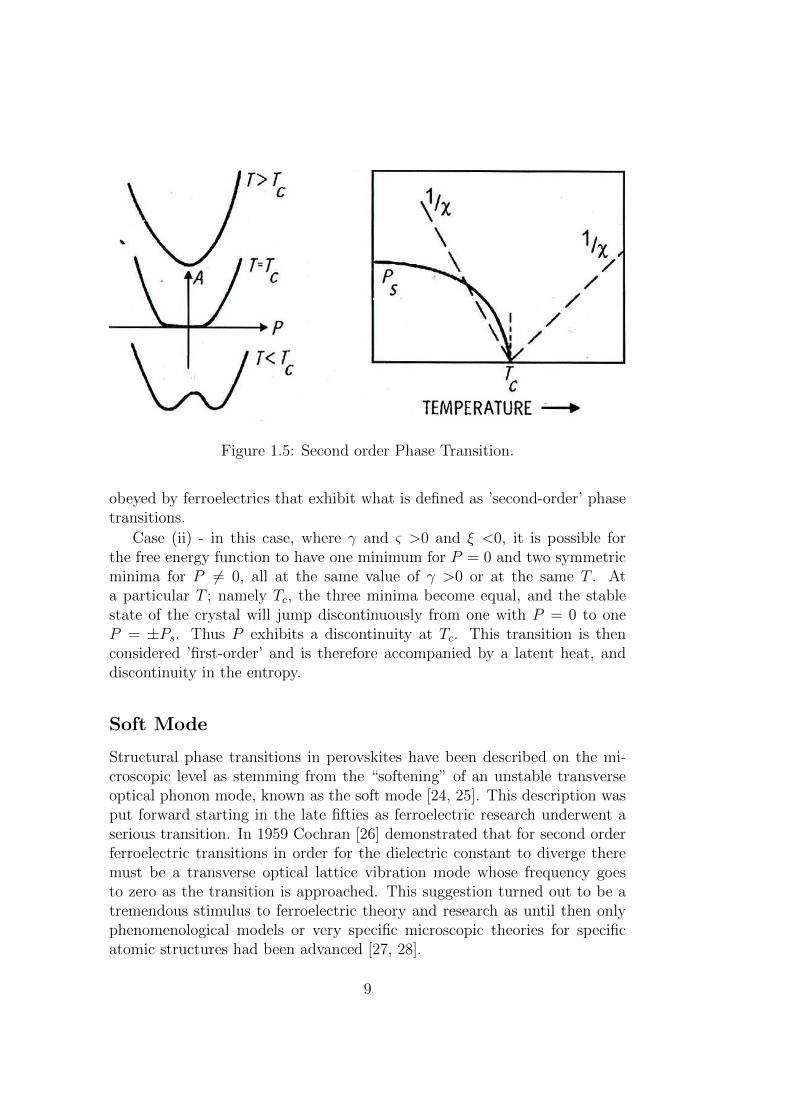
Figure 1.5: Second order Phase Transition.
obeyed by ferroelectrics that exhibit what is defined as ’second-order’ phasetransitions.
Case (ii) - in this case, where γ and ς >0 and ξ <0, it is possible forthe free energy function to have one minimum for P = 0 and two symmetricminima for P 6= 0, all at the same value of γ >0 or at the same T . Ata particular T ; namely Tc, the three minima become equal, and the stablestate of the crystal will jump discontinuously from one with P = 0 to oneP = ±Ps. Thus P exhibits a discontinuity at Tc. This transition is thenconsidered ’first-order’ and is therefore accompanied by a latent heat, anddiscontinuity in the entropy.
Soft Mode
Structural phase transitions in perovskites have been described on the mi-croscopic level as stemming from the “softening” of an unstable transverseoptical phonon mode, known as the soft mode [24, 25]. This description wasput forward starting in the late fifties as ferroelectric research underwent aserious transition. In 1959 Cochran [26] demonstrated that for second orderferroelectric transitions in order for the dielectric constant to diverge theremust be a transverse optical lattice vibration mode whose frequency goesto zero as the transition is approached. This suggestion turned out to be atremendous stimulus to ferroelectric theory and research as until then onlyphenomenological models or very specific microscopic theories for specificatomic structures had been advanced [27, 28].
9

Figure 1.6: First order Phase Transition.
Figure 1.7: Soft mode of Nb ion vibrations inside the KTN lattice.
10
1.2.3 Polar Nanoregions and Relaxor Ferroelectrics
As mentioned within the ferroelectric crystal the unit cell is slightly distortedand contains a microscopic electrical dipole moment. Neighboring unit celldistortions may form domains of correlated displacement creating a macro-scopic dipole moment along a particular preferred crystallographic directionresulting from some anisotropic distortions of the symmetric cubic lattice.These moments will persist even in the absence of an electric field. Above acertain temperature the macroscopic polarization properties will vanish al-though there may still be various nanoregions in which on a microscopic levelthere is still a dipole moment. The temperature at which these nanoregionsbegin to form is known as the Burns temperature [29] and is often designatedTd. An additional temperature of note has been recently called the interme-diate temperature [30] and denoted T ∗. It is at this temperature that thedifferent polar nanodomains begin to interact with one another and displaysigns of correlative behavior.
1.2.4 The Ferroelectric Material - KTN
Ferroelectric Potassium Tantalate Niobate (KTN) was one of the first crystalsrecognized as possessing photorefractive properties [31]. Consequently it andits derivatives, such as Potassium Lithium Tantalate Niobate (KLTN), havebeen the subject of much study because of their applicability in Electro opticapplications [32]. Of particular interest was the possibility to exploit them asoptical switches based on electrically controlled volume holograms [33, 34].However, their full potential has never been realized because of the dynamicsof volume holograms [31]. In KLTN a possible mechanism was traced to theformation of metastable ferroelectric clusters in the paraelectric phase [35,36]. Volume holography depends on the birefringence, ∆n, of the crystal.
∆n (r) =1
2geffP
2 (r) =1
2geff [(ε− 1)E (r)]2 , (1.2)
where r is the position vector in crystal, geff is the effective electro-opticalcoefficient of the crystal, ǫ is the low frequency dielectric permittivity andE is the low frequency internal electric field. As clusterization will naturallyaffect the dielectric permittivity the original purpose of this thesis was toinvestigate the dynamics of clusterization of various dopants inside KTN andKLTN. While the effect of impurities on the gross dielectric behavior of KTNhad been noted [37, 36] the dielectric response of the impurities had not beenaddressed. The point is important because while the optical properties of acrystal may be improved by adding an impurity, the impurity itself becomes
11

Figure 1.8: Eight site model of the central Niobium position inside KTN. Offcenter positions are shown for all four phases, with the arrow indicating thedirection of the dipole moment.
a dispersive center within the ordered crystal lattice. Consequently it willhave its own dynamic behavior in the dielectric response. As all practicalapplications of these crystals will be limited by the time window of operation,the dielectric response in that window will be a dominating factor whenevaluating application efficacy. Additionally, by exploiting specific frequencybased features of the dielectric relaxation, it may be possible to develop noveloptical uses for the doped crystals.
KTN crystals belong to the class of Perovskite crystals. The basic unitcell is simple and is illustrated in Figure . The general formula for the unitcell is ABO3, where A signifies the corner monovalent or divalent ions andB the ion occupying the center of inversion of the cell, usually tetravalentor pentavalent. The oxygen ions positioned at the face centers comprise arigid octahedra. However, this structure is sometimes given to tilting, leadingto structural transitions that are not ferroelectric. One example of such asystem which undergoes a number of non-ferroelectric transitions, related tothis tilt of the octahedra, is NaNbO3 [20].
12
More central to the dynamics in KTN, is the Niobium B ion, whichcan be found in off-center positions around the center of inversion. It isthis off centering which leads to the presence of dipoles and therefore toferroelectric phenomena. The presence of off centering of the B ion usuallyimplies that the perovskites are in fact highly polarizable dielectric media.This is significant when considering the ordering of impurity dipoles at low,or even trace concentrations in such media.
1.3 Physics of Dielectrics
1.3.1 Dielectric Mechanisms
There are a number of different dielectric mechanisms, connected to the way astudied medium reacts to an applied electric field. Each dielectric mechanismis centered around its characteristic frequency, which is the reciprocal of thecharacteristic time of the process. In general, dielectric mechanisms can bedivided into relaxation and resonance processes. The most common, startingfrom high frequencies, are:
1. Electronic polarization
This resonant process occurs when the electric field displaces the nega-tively charged electron density relative to the positively charged nucleuswhich it surrounds. This displacement hinges upon the delicate equi-librium between restoration and electric forces. Electronic polarizationmay be understood by assuming an atom as a point nucleus surroundedby a spherical electron cloud of uniform charge density.
2. Atomic polarization
Atomic polarization is observed when the nucleus of the atom reorientsand changes its dipole direction in response to an applied electric field.This too is a resonant process intrinsic to the nature of the atom anda direct consequence of an applied electric field. Atomic polarization isusually small compared to electronic polarization.
3. Dipole relaxation
This process originates from both permanent and induced dipoles align-ing with an electric field. Their orientational polarization is disturbedby thermal noise introducing misalignment between the dipole vectorsand the direction of the electric field. The time needed for dipoles torelax is determined by the local viscosity. Dipole relaxation is therefore
13

Figure 1.9: Regimes of dielectric relaxation with emphasis on the differentmechanisms and noting their typical frequency bands.
heavily dependent on the temperature, pressure and chemical surround-ings.
4. Ionic relaxation
Ionic relaxation is comprised of ionic conductivity as well as interfacialand space charge relaxation. Ionic conductivity predominates at lowfrequencies introducing only losses to the system visible in the imagi-nary part of the dielectric response. Interfacial relaxation occurs whencharge carriers are trapped at interfaces of heterogeneous systems. Arelated effect is Maxwell-Wagner-Sillars polarization [38], where chargecarriers blocked at inner dielectric boundary layers (on the mesoscopicscale) or external electrodes (on a macroscopic scale) lead to a sep-aration of charges. The charges may be separated by a considerabledistance and therefore make contributions to the dielectric loss that areorders of magnitude larger than the response due to molecular fluctu-ations.
Having determined that there are indeed a number of different mecha-nisms which can be responsible for the dielectric response of a material thenext task is to differentiate between some of their different features in order toallow identification of a specific mechanism under particular circumstances.
14

In general the procedure will be to measure the dielectric response, and thenseparate the different processes using fitting functions which will be describedshortly. Finally, based on the fitting parameters and their dynamic behaviorin response to pressure/temperature/compositional changes, determine whatis the underlying mechanism governing the behavior.
In order to distinguish between the different mechanisms and properlyidentify the factors responsible for a given dielectric process we must firstextract the relaxation parameters by fitting the dielectric response with anappropriate fitting function. The measurements themselves and the accom-panying fitting procedure can be undertaken in one of two domains. Theycan be Frequency domain measurements, measuring the response to oscillat-ing input at various frequencies, or Time domain measurements measuringthe direct time varying response to a fast rising impulse.
1.3.2 Dielectric Response in the Frequency Domain
Measurement Theory
When placed in an external electric field E , a dielectric sample acquiresa non-zero macroscopic dipole moment. This means that the dielectric ispolarized under the influence of the electric field. The polarization P of thesample, or dipole density, can be presented in a very simple way
P =〈M〉V
, (1.3)
where <M> is the macroscopic dipole moment of the whole sample volumeV, which is formed by the permanent micro dipoles (i.e. coupled pairs ofopposite charges) as well as by dipoles that are not coupled pairs of microcharges within the electro neutral dielectric sample. The brackets < > denoteensemble average. In a linear approximation the macroscopic polarization ofthe dielectric sample is proportional to the strength of the applied externalelectric field E :
Pi = ε0χikEk (1.4)
where χik is the tensor of the dielectric susceptibility of the material andǫ0 =8.854·10−12[F·m−1] is the dielectric permittivity of the vacuum. If thedielectric is isotropic and uniform, χ reduces to a scalar and equation (1.4)will be reduced to the more simple form:
P = ε0χE (1.5)
For simplicity the following discussion will be considered for isotropicmediums only. When the electric field is turned on at t=0 then the polariza-tion P will begin to grow until it reaches its equilibrium value as governed by
15

equation 1.4. This process is not instantaneous. Likewise when the electricfield E is removed in a step wise fashion the induced Polarization will beginto decay [39]. This relaxation can be described by a relaxation function:
α(t) =P (t)
P (0)where α(0) = 1 and α(∞) = 0. (1.6)
More generally the relationship between a time dependent Electric field andthe Polarization it induces is given by:
P(t) = χ
∫E(t′)φp(t− t′)dt′. (1.7)
where the relation between the step response relaxation function, α(t) andφp(t) is given by−α(t) = φp(t). φp(t) is known as the pulse response function,accordingly.
The displacement field D(t) induced in the medium as a result of E(t)and P(t) is given by the familiar equation:
D(t) = ε0E(t) +P(t). (1.8)
For a uniform isotropic dielectric medium, the vectors D, E, P have thesame direction, and the susceptibility is coordinate-independent, therefore
D(t) = ε0(1 + χ)E(t) = ε0εE(t). (1.9)
where ε = 1+χ is the relative dielectric permittivity. Traditionally, it is alsocalled the dielectric constant, because in a linear regime it is independent ofthe field strength. However, in practice it is almost always a function of manyother variables. For example in the case of time variable fields it is dependenton the frequency of the applied electric field, sample temperature, sampledensity (or pressure applied to the sample), sample chemical composition,etc.
Incorporating the time dependence into equation 1.8 above will producethe relation between the displaement vector D(t) and the electric field E(t)giving us
D (t) = ε0
[ε∞E (t) +
∫ t
−∞
•Φ(t
′)E (t− t′) dt′]. (1.10)
now Φ(t) is the dielectric response function
Φ(t) = (εs − ε∞)[1− φ(t)]. (1.11)
using εs = ε∗ (0) and ε∞ = ε∗ (∞) as the static and high frequency limits ofthe dielectric permittivity.
16
Under these conditions the normalized dielectric susceptibility is
χN(ω) =χ(ω)
χ(0)=ε∗(ω)− ε∞
∆ε. (1.12)
The real part, ε’(ω), is referred to as the frequency dependent dielectricpermittivity and in the low frequencies is a monotonically decreasing functionof frequency. As can be inferred from equation 1.10 it is equal to the realcomponent of the Laplace transform of the pulse response function.
ε′ (ω) = ε∞ +∆ε
∫ ∞
0
cos (ωt)φorp [t] dt. (1.13)
The imaginary part of the complex dielectric permittivity often referred toas the loss factor and is related to the work done [39], by the Electric fieldin the dielectric media:
ε′′ (ω) = ∆ε
∫ ∞
0
sin (ωt)φorp [t] dt (1.14)
If W is the average energy dissipation per unit time then
W (ω) =ωE2
0
8πε” (ω) , (1.15)
where E0 is the amplitude of the sinusoidal impinging electric field. Atfrequencies below f ≤ 1013Hz the source of polarization is due to the re-orientation of dipoles with the impinging electric field. The correspondingamplitude of the real component of the dielectric permittivity is proportionalto the number of orientated dipoles at that frequency, while the gradient re-flects the rate of change in their number. Consequently the gradient is relatedto the energy dissipation in order to reorient a dipole and therefore to theimaginary component, often referred to as the dielectric losses. In the firstorder approximation this is expressed by the relationship
ε′′ (ω) ≈ ∂ε′ (ω)
∂ logω. (1.16)
More formally this is simply the first approximation of the Kramers- Kronigrelationships [40]:
ε′(ω0) = ε∞ +1
π
∫ ∞
0
ωε′′(ω)
ω2 − ω20
dω (1.17)
and
ε′′(ω0) =2ω0
π
∫ ∞
0
ε′(ω)
ω2 − ω20
dω. (1.18)
17

Debye Relaxation
Debye relaxation is in effect, the dielectric relaxation response of an ideal,noninteracting population of dipoles to an alternating external electric field.It is usually expressed as the complex permittivity of a medium, as a functionof the field’s frequency:
ε∗(ω) = ε∞ +εs − ε∞
[1 + (iωτm)], (1.19)
where ε∞ is the permittivity at the high frequency limit, εs is the staticlow frequency permittivity, and τm is the characteristic relaxation time ofthe medium. This relaxation model was introduced by and named afterthe chemist Peter Debye (1913) and adequately describes the simplest formof relaxations [41]. Some of the methods of measuring this parameter alongwith the underlying theory behind them will be presented later on in Chapterthree.
For many of the systems being studied, the relationship above howeverdoes not sufficiently describe the experimental results. The Debye conjectureis much too simple and elegant. While enabling us to understand the natureof dielectric dispersion it cannot provide a full picture encompassing all ofthe system’s complexities. In many instances the experimental data is betterdescribed by non-exponential relaxation laws. This necessitates empiricalrelationships, which formally take into account the distribution of relaxationtimes.
Phenomenological Models of Non-Debye Relaxation
More commonly observed in practice however are the more complicated,widespread, non-Debye relaxation behaviors. These are observed in a widevariety of complex materials, some examples of which are polymers, mi-croemulsions, associated liquids, sol-gel glasses, different porous systems, andalso ferroelectric crystals.
In these cases, the experimentally measured dielectric spectrums are bestdescribed by the so-called Havriliak-Negami (HN ) empirical relationship [42]
ε∗(ω) = ε∞ +εs − ε∞
[1 + (iωτm)α]β
α, β < 1, (1.20)
Here α and β are empirical exponents. The specific case α=1, β=1 givesthe Debye formula, β=1, α 6=1 corresponds to the so-called Cole-Cole (CC)equation [43], whereas the case α=1, β 6=1, corresponds to the Cole-Davidson(CD) equation [44].
18
Sometimes in the case of superposition of relaxation processes with dc andac conductivity the high and low frequency asymptotic forms may be assignedto Jonscher’s power-law wings (iωτi)
(ni−1) (where ni is a Jonscher exponent,and τi is the corresponding characteristic relaxation time) [11]. Notice thatthe real part ǫ′(ω) of the complex dielectric permittivity is proportional tothe imaginary part σ”(ω) of the complex ac conductivity σ ∗ (ω), ε′(ω) ∝−σ′′(ω)/ω, and the dielectric losses ǫ′′(ω) is proportional to the real part σ′(ω)of the ac conductivity, ε′′(ω) ∝ σ′(ω)/ω. The latter arises from the Johnscherterm and has the form, σ′(ω) ∝ ωuj , which has been termed “universal” dueto its appearance in many types of disordered systems [45].
1.3.3 Dielectric Response in the Time Domain
An alternative approach is to obtain information on the dynamic molecularproperties of the substance directly in the time domain.
When an external field is applied to a dielectric, polarization of the ma-terial reaches its equilibrium value, not instantaneously, but rather over aperiod of time. By analogy, when the field is suddenly removed, the polar-ization decay caused by thermal motion follows the same law as the relaxationor decay function of dielectric polarization φ(t):
φ (t) =P(t)
P(0). (1.21)
where P is a polarization vector of a sample unit. The relationship forthe dielectric displacement vector D(t) in the case of time dependent fieldsmay be written as follows:
D (t) = ε0
[ε∞E (t) +
∫ t
−∞
•Φ(t
′)E (t− t′) dt′]. (1.22)
In the above equation D (t) = ε0E (t) + P (t), and Φ(t) is the dielectricresponse function, where ǫs and ǫ∞ are the low and high frequency limitsof the dielectric permittivity, respectively. The complex dielectric permittiv-ity ǫ* (ω) (with ω denoting the angular frequency) is connected with therelaxation function by a very simple relationship:
ε∗(ω)− ε∞εs − ε∞
= L
[− d
dtφ (t)
]. (1.23)
L is the operator of the Laplace transform, which is defined for an arbitrarytime-dependent function f (t) as:
L [f(t)] ≡ F (ω) =
∫ ∞
0
e−ptf(t)dt. (1.24)
19

with p = x+ iω, as x→ 0.Relation (1.23) shows that equivalent information will be obtained when
measuring dielectric relaxation properties, whether it is being tested eitherin the frequency or time domain. Therefore the dielectric response may bemeasured experimentally as a function of frequency or time, in both casesproviding data in the form of a dielectric spectrum ε∗ (ω) either directly ofvia transform of the macroscopic relaxation function φ (t).
For example, when macroscopic relaxation function obeys the simple ex-ponential law
φ(t) = exp(−t/τm), (1.25)
with τm representing the characteristic relaxation time, the well-known De-bye formula for the frequency dependent dielectric permittivity can be ob-tained by substitution of (1.25) into (1.23).
Dipole Correlation Function
Polarization fluctuations caused by thermal motion in the linear responsecase are the same as for macroscopic reconstruction induced by the electricfield [46]. This means that one can equate the macroscopic dipole correlationfunction:
ϕ (t) ∼= Ψ(t) =〈M (0)M (t)〉〈M (0)M (0)〉 , (1.26)
where M (t) is the macroscopic fluctuation dipole moment of the samplevolume unit which is equal to the vectorial sum of all the molecular dipoles;and the symbol < > denotes averaging of the ensemble. Both the velocityand the laws governing the macroscopic dipole correlation function (DCF )are directly related to the structural and kinetic properties of the sample andcharacterize the macroscopic properties of the studied system.
In the linear response approximation, the fluctuations of polarizationcaused by thermal motion are the same as for the macroscopic rearrange-ments induced by the electric field. Thus, one can equate the relaxationfunction φ(t) and the macroscopic dipole correlation function (DCF ) Ψ(t)as follows:
φ(t) ∼= Ψ(t) =〈M (0)M (t)〉〈M (0)M (0)〉 , (1.27)
where M (t) is the macroscopic fluctuating dipole moment of the sample vol-ume unit, which is equal to the vector sum of all the molecular dipoles. Therate and laws governing the DCF are directly related to the structural andkinetic properties of the sample and characterized the macroscopic properties
20

of the system under study. Thus, the experimental function Φ(t) and henceφ(t) or Ψ(t) can be used to obtain information on the dynamic properties ofthe dielectric under investigation.
An alternative approach is to obtain information on the dynamic molec-ular properties of the substance directly in the time domain. Polarizationfluctuations caused by thermal motion in the linear response case are thesame as for macroscopic reconstruction induced by the electric field [47].Therefore one can equate the macroscopic relaxation function Ψ(t) and themacroscopic dipole correlation function Γ(t):
Ψ(t) = Γ (t) =〈M (0) ·M (t)〉〈M (0) ·M (0)〉 . (1.28)
The rate and laws governing the decay function, Γ(t), are directly relatedto the structural and kinetic properties of the sample and characterize themacroscopic properties of the system studied.
1.4 Interpreting the Dielectric Response
1.4.1 Origin of Non-Debye Relaxation
Of the three models presented (CC, CD, HN) only the Debye model currentlyhas an accepted physical meaning, relating to the relaxation of a dipole in aMaxwellian field generated by the remaining dipoles of the medium. With nointeraction even between nearest neighbor dipoles, and the resulting polar-ization interpreted in terms of a mean field, the relaxation will be exponentialin nature, leading to the Debye formula [11].
This can be derived in the following way. Considering a set of dipoles,with dipole moment µ in a crystalline field with a discrete number of possibleorientations, each separated by a potential barrier. In the simplest case thereare only two, opposing directions. If n1 is the number of dipoles in directionone and n2 is the number of remaining dipoles then a rate equation can bewritten [48]
d
dt(n1 − n2) = − (ν21 + ν12) (n1 − n2) , (1.29)
where νij is the probability of a dipole orientating from direction i to j perunit time. Recognizing νij as a time constant the time evolution of n1 andn2 will be governed by
(n1 − n2) = f0 exp (−t/τ) , (1.30)
21

where n = n1+n2 is constant , f0 is the initial population difference andτ = (ν21 + ν12)
−1. If an external constant field E is applied and then closedat the moment t=0 the resultant polarization in the direction of the field willbe given by
P(t) = 〈µ (n1 − n2)〉 = µ (n1 − n2)
[cosh
(µE0
kBT
)− 1
]≈ µ2E0
kBTexp (−t/τ) .
(1.31)E0 is the amplitude of the electric field and the ensemble of dipoles is averagedaccording to the Boltzmann energy distribution. In this distribution theenergy, V = E0µcos (θ) , of the system is defined as the scalar product of thedipole moment,µ, and the impinging field, E0, with θ the angle between them.The last term is derived using equation (1.30), while assuming µE0/kBT <<1. The susceptibility is then given by the Debye expression
χ (ω) =µ2
kBT
1
1 + iωτ. (1.32)
The Debye equation describes the reorientation over a potential barrier ofnon interacting dipoles. The driving force is simply thermal interactionswith a heat bath. Implicit in the expression is a single relaxation time forall dipoles in the ensemble. Assuming all potential barriers to be equivalentthen the behavior of the relaxation times as a function of temperature willbe Arrhenius
τ = τ0 exp
(∆V
kBT
), (1.33)
where ∆V is the barrier height and τ 0 is the defining period of the relaxationtime.
As mentioned above a significant number of systems demonstrate devia-tions from Debye behavior leading to CC [43] or CD [44] expressions for thedielectric permittivity. Phenomenologically these expressions can be achievedif the assumption of a single uniform relaxation time is relaxed and replacedby a distribution function, f(τ) for a set of Debye functions. The correctbehavior is obtained by
χ (ω) = χ′ (0)
∫ ∞
0
dτf (τ)
1 + iωτ. (1.34)
The distribution functions for the CC and CD functions can be found inRef. [11]. Implicit in this description is a continuous distribution of bar-rier heights. Such an approach is unable to explain temperature behaviorof the parameters such as α and β, or illuminate the microscopic causes of
22

anomalous dielectric relaxation. An alternative more complicated yet morecomprehensive approach employs fractional derivatives and memory func-tions.
1.4.2 Fractional Derivatives
The Debye treatment of dielectric relaxation assumes one time scale for a sin-gle reorientation. This idea is analogous to Einstein’s treatment of Brownianmotion using a Random Walker approach. A more realistic model allows thedipole an arbitrary long waiting period between reorientations. Assumingthat the waiting times are described by a probability distribution function,W (φ, t) where the orientation, φ, of the dipole and the waiting times areindependent of each other one can obtain the following fractional derivativeequation
∂W (φ, t)
∂t= −τ−α
0 0D1−αt
∂2
∂φ2W (φ, t) , (1.35)
where
0D1−αt g (t) =
1
Γ (α)
∂
∂t
∫ t
0
g (t′)
(t− t′)1−α . (1.36)
Here g(t) is an arbitrary function, Γ(α) is the gamma function τ0 is a constantand 0<α<1. Expression 1.36 is known as the Riemann-Liouville fractionalderivative operator.
1.4.3 The Cole-Cole Equation
Ryabov and Feldman [49] have exploited the Mori-Zwanzig projection method-ology, coupled with the fractional derivative formalism to explain the micro-scopic origin of CC behavior in some glass formers specifically nylon-6,6. Us-ing f(t) as the normalized correlation function corresponding to an anomalousdielectric relaxation, its time dependence can be expressed using a memoryfunction m(t) such that
df (t)
dt= −
∫ t
0
m(t− t′)f(t′)dt′. (1.37)
Taking into account relationship and equating the Laplace transform of f(t)to equation (1.20) with β=1 and 0<α<1 , the Laplace transform of thememory function for the CC expression is
M (z) = L(m(t)) = z1−ατ−α. (1.38)
23

Using the above equation (1.38) with the Riemann-Liouville fractional deriva-tive operator,0D
1−αt , as defined in equation (1.36) they were able to express
the memory function (equation (1.37)) in terms of a fractional derivativeequation
df (t)
dt= −τ−α
0D1−αt [f (t)] . (1.39)
The consequence of this equality is that a fractional memory effect underpinsthe Riemann-Liouville operator. Furthermore they related the microscopicrelaxation of a unit in the relaxing ensemble to an individual memory functionfrom a summation of delta functions mδ(t) ∼ ∑
i δ (ti − t), describing inessence the interrupted interaction of the unit with its surroundings. If thesequence of ti is a fractal set, such that for some scale transformation itremains invariant, then the ensemble average in the interval [λt, t ] is givenby
m (t) =
∫ 1/2
−1/2
mδ
(λ−ut
)λ−u(1−df )du, (1.40)
where df is the fractal dimension of the set and the Laplace transform ofm(t) takes the form
M(z) ∼ z1−df . (1.41)
The similarity between equations (1.41) and (1.38) leads to the conclusionthat df=α and that the broadening of the peak from Debye behavior is aresult of the interaction between the microscopic elements of the ensemblewith their surroundings. The parameter α in the CC equation is the fractaldimension of the time set defined by
α =ln(N)
ln(ξ), (1.42)
where N is the number of interactions in the time set defined by the dimen-sionless time parameter ξ. For transport processes involving self diffusionthey derived a simplified relationship between the structural parameters ofthe system and the parameters of the CC equation
α =DG
2
ln (τωc)
ln (τ/τ0), (1.43)
where DG is the spatial fractal dimension, τ the relaxation time for theprocess, ωc is the characteristic frequency for the self diffusive transport andτ 0 is a microscopic cut off time for the diffusive process.
The specific type of diffusion required to reproduce the exact form de-scribed in the Cole-Cole equation is not the normal diffusion with a squared
24
dependence on diffusion length but rather a slightly more anomalous version.One of the possible origins for this anomalous behavior is the appearance ofergodicity breaking [50, 51].
1.4.4 Ergodicity Breaking
The ergodic hypothesis is one of the cornerstones of statistical mechanics.It states that ensemble averages and time averages are equal in the limitof infinite measurement time. In other words, over long periods of time,the time spent by a particle in some regions of the phase space with equalenergy is proportional to the volume of these regions. This ensures that allaccessible microstates are ultimately equally probable when measuring overa long period of time. The term ergodic is then used to describe a dynamicalsystem which, broadly speaking, has the same behavior averaged over timeas averaged over the space of all the system’s states (phase space) [52].
In macroscopic systems, the timescales over which a system can truly ex-plore the entirety of its own phase space can be sufficiently large that the ther-modynamic equilibrium state exhibits some form of ergodicity breaking. Acommon example is that of spontaneous magnetization in ferromagnetic sys-tems, whereby below the Curie temperature the system preferentially adoptsa non-zero magnetization even though the ergodic hypothesis would implythat no net magnetization should exist by virtue of the system exploringall states whose time-averaged magnetization should be zero. The fact thatmacroscopic systems often violate the literal form of the ergodic hypothesisis an example of spontaneous symmetry breaking.
However, complex disordered systems such as a spin glass show an evenmore complicated form of ergodicity breaking where the properties of thethermodynamic equilibrium state seen in practice are much more difficultto predict purely by symmetry arguments. In practice, this means that onsufficiently short time scales (e.g. those of parts of seconds, minutes, or a fewhours) the systems may behave as solids, i.e. with a positive shear modulus,but on extremely long scales, e.g. in millennia or eons, as liquids, or withtwo or more time scales and plateaux in between.
Starting with the work of Bouchaud [53], there has been growing interestin weak ergodicity breaking, with applications in a wide range of physicalsystems: phenomenological models of glasses, laser cooling, blinking quan-tum dots, and models of atomic transport in optical lattices. Weak ergodicitybreaking is found for systems whose dynamics is characterized by power lawsojourn times, with infinite average waiting times. In such systems the mi-croscopical time scale diverges, for example, the average trapping time of anatom in the theory of laser cooling. The relation between ergodicity breaking
25

and diverging sojourn times can be briefly explained by noting that one con-dition to obtain ergodicity is that the measurement time is long, comparedwith the characteristic time scale of the problem. However this conditionis never satisfied if the microscopical time scale, i.e., the average trappingtime, is infinite. It was introduced into physics by Scher and Montroll inthe context of continuous-time random walk (CTRW) [54]. This well knownmodel exhibits anomalous subdiffusion and aging behaviors which are relatedto ergodicity breaking.
There is therefore a direct link between ergodicity breaking and Cole-Colerelaxation. This does not necessarily mean however, that any appearance ofCole-Cole relaxation immediately implies non-ergodicity [55]. For Cole-Colebehavior the Anomalous diffusion produced by a fractal underlying latticecould suffice, without having to incur a model with real ergodicity breaking.As pointed out already by Bouchaud [53] in order to clearly demonstrateergodicity breaking it is necessary to measure the system’s ageing properties.
Ageing in Non-Ergodic Systems
The term ageing was originally coined in relation to the non-stationary, out-of-equilibrium behaviour observed in glassy systems. It is used to describethe fact that probing such systems at some (ageing) time ta after the sys-tem’s initial preparation (at time t = 0) changes the measured results (i.e.relaxation times). This will happen in systems where the rate of changingstates typically increases with t (for sufficiently long observation periods).Power-law distributed waiting times, for example, can lead to this kind ofageing in a wide variety of systems. The evolution of the subdiffusive behav-ior in these cases, will start to include longer and longer waiting time eventsso that as we start to observe the particle at later and later ageing times,we will be more likely to find it within one of these extremely long waitingperiods.
Ageing is thus a symptom on weak ergodicity breaking and is thereforea well defined method of investigating and characterizing such systems. Itintroduces a new control variable in the form of ta which can help providemore information on the system. If the system does indeed undergo ageingthan the correlation functions themselves will not be static but time evolving.
Ageing in Disordered Dielectrics
Ageing in disordered dielectrics has been studied in a number of systems [3,56, 57, 58, 59]. The ergodicity breaing in these instances is attributed tothe low-temperature states with frozen-in polarization devoid of long range
26

ferroelectric order [3]. Different mechanisms are active in various lead basedrelaxors including effects due to domain structure stabilization. More specif-ically, ageing in ferroelectric KTN has been observed in the low Nb crystals[60, 61] where KTN still exhibits relaxor behavior.
The model proposed in the thesis to describe the electron hopping be-havior is not dependent on the presence of true ergodicity breaking. Evena system such as KTN composed of these fractal nanodomains would sufficeto produce the hopping behavior as observed. We therefore don’t think itis necessary to expand too much on the topic of ageing. As noted, it seemsunlikely that these crystals will exhibit appreciable ageing effects.
The question of whether or not there is true ergodicity breaking is ex-tremely important [62] but also much too broad to be covered within theframework of this thesis.
1.4.5 The Kohlrausch-Williams-Watts Relaxation Law
The deviation from the classical exponential Debye function which producesthe Cole-Cole frequency domain relaxation as described above, can be alter-natively described by various functions in the time domain directly. The mostcommonly used empirical relaxation function in these cases is the stretched-expoential, known as the Kohlrausch-Williams-Watts (KWW) relaxation law[63, 64].
ψ(t) = Ae−(t/τM
)ν
. (1.44)
where τM is the macroscopic relaxation time, and 0 < ν ≤ 1 is the stretch-ing exponent. The fact that KWW relaxations are frequently observed hasmotivated an in-depth search for generating mechanisms.
The KWW decay function can be considered as a generalization of thatbecomes Debye’s law when ν = 1. The fact that KWW relaxations are fre-quently observed has motivated search for generating mechanisms. In crys-talline solids the KWW has frequently been linked to transport mechanismssuch as electron hopping [65].
Power and Stretch
Although the KWW law is quite common, it is actually only one of a seriesof theoretically predicted relaxation forms. Further examples of time domainrelaxation functions used to model the relaxation behavior, include
27

1. The Algebraic Form (Power Law) [66]
ψ(t) = A(t/τ1
)−µ
. (1.45)
with an amplitude A, an exponent µ > 0 and a characteristic time τ1which is associated with the effective relaxation time of the microscopicstructural unit; This relaxation power law is sometimes referred bythe literature as describing anomalous diffusion when the mean squaredisplacement does not obey the linear dependency < R2 >∼ t. Instead,it is proportional to some power of time < R2 >∼ tγ (0 < γ < 2). Inthis case, the parameter τ1 is an effective relaxation time required forthe charge carrier displacement on the minimal structural unit size. Anumber of approaches exists to describe such kinetic processes.
2. Exponential-Logarithmic Expression [67]
ψ(t) ∼ explnγ(t/τM
). (1.46)
3. The Inverse Logarithm
ψ(t) ∼ ln−γ(t/τM
). (1.47)
4. The product of both the KWW and power-law
ψ(t) = A(t/τ1
)−µ
exp−(t/τM
)ν. (1.48)
this type of relaxation law is an important example of a phenomenolog-ical decay function that has different short- and long-time asymptoticforms [50].
In the time domain an expression analogous to the HN function doesnot exist. The relationship between the parameters of HN equation in thefrequency domain and stretch-on-power law in the time domain seems tobe useful only asymptotically. The meaning of these functions in the timedomain must therefore be explained differently than in the frequency domain.A connection can be made between these functions and the description ofpercolation in complex materials.
28

Figure 1.10: Bond percolation.
1.4.6 Percolation
Percolation refers to the formation of long-range connectedness or conduc-tivity in random systems. Simple models for percolation were independentlydevised in the areas of polymer science and mathematics in the 1940s and’50s, and have been both a persistent theoretical challenge and an enduringpractical paradigm ever since. In the past two decades, percolation has be-come a central problem in probability theory, and has figured in the work oftwo recent Fields medalists [68, 69].
At its heart, percolation is a simple probabilistic model which also ex-hibits a phase transition making it a natural choice when trying to finda comprehensive model of the ferroelectric PT. The simplest version takesplace with cells on a square lattice, each square, independently of its neigh-bors, chosen to be occupied with probability p and empty with probability1−p. The basic question in this model is: What is the probability that thereexists an infinite cluster, i.e., a path all of whose cells are occupied, from theone end to the other? Figure 1.10 shows the parallel case where the sitesare occupied but the connection or “bond” between the two is some type ofprobability distribution. The occupation probability p at which this infinitepath becomes manifest (the probability increases dramatically) is defined asthe the critical concentration pc.
In standard percolation, the probability P∞ that a given point is part of apercolating cluster is a continuous function of the site occupation probabilityp, the probability that a site is occupied or empty. P∞ is zero for cases where
29
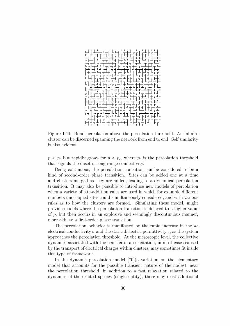
Figure 1.11: Bond percolation above the percolation threshold. An infinitecluster can be discerned spanning the network from end to end. Self similarityis also evident.
p < pc but rapidly grows for p < pc, where pc is the percolation thresholdthat signals the onset of long-range connectivity.
Being continuous, the percolation transition can be considered to be akind of second-order phase transition. Sites can be added one at a timeand clusters merged as they are added, leading to a dynamical percolationtransition. It may also be possible to introduce new models of percolationwhen a variety of site-addition rules are used in which for example differentnumbers unoccupied sites could simultaneously considered, and with variousrules as to how the clusters are formed. Simulating these model, mightprovide models where the percolation transition is delayed to a higher valueof p, but then occurs in an explosive and seemingly discontinuous manner,more akin to a first-order phase transition.
The percolation behavior is manifested by the rapid increase in the dcelectrical conductivity σ and the static dielectric permittivity ǫs as the systemapproaches the percolation threshold. At the mesoscopic level, the collectivedynamics associated with the transfer of an excitation, in most cases causedby the transport of electrical charges within clusters, may sometimes fit insidethis type of framework.
In the dynamic percolation model [70](a variation on the elementarymodel that accounts for the possible transient nature of the nodes), nearthe percolation threshold, in addition to a fast relaxation related to thedynamics of the excited species (single entity), there may exist additional
30
relaxations with much longer characteristic time scales associated with therearrangement of the typical percolation cluster as well as the cooperative re-laxation phenomenon associated with the transport of charge carriers alongthe percolation cluster .
Due to the cooperative nature of relaxation, the DCF decay behavior con-tains information regarding the transient cluster morphology at the mesoscalethat reflects the dynamical character of percolation. The type of the relax-ation law seen in such cases in the time domain is strongly dependent on thedistance from the percolation threshold. In general far from the thresholdthe relaxation is dominated by a fractional power law:
Ψ(t) ∝ (t/τ 1)−µ. (1.49)
In the vicinity of the percolation threshold, the relaxation law changes frompower law to behavior including a stretched exponential in the form of,
Ψ(t) ∝ exp[-(t/τm)ν ] (1.50)
The actual behavior that develops starting in this crossover region is arelaxation law is best approximated as a product of both the power law andstretched exponential, as described by:
Ψ(t) ∝ (t/τ 1)−µ exp[-(t/τm)
ν ]. (1.51)
The magnitude of parameter µ will decrease to almost zero as the temper-ature approaches that of the percolation threshold. Confirming the statementmentioned above that at the percolation threshold temperature the behaviorof the dipole correlation function is of the KWW type. The decay of theDCF ψ(t) is governed mainly by the power law.
The relaxation time, τm/τ1 and the amplitude A correspond to the macro-scopic relaxation time of the decay function determined above [12]. Near thepercolation threshold, τm/τ1 exhibits a maximum and reflects the well-knowncritical slowing down effect. The description of the mechanism of the coop-erative relaxation in the percolation region.
A description of the dielectric response in the vicinity of the percolationthreshold has been developed within the framework of the regular fractalmodel. The model originally developed for percolation processes in ion mi-croemulsions and porous borosilicate glasses [71] is nonetheless, completelygeneral and allowing us to apply the main results to any disordered media.From the analysis of dielectric relaxation parameters of the percolation pro-cess we can obtain the geometrical characteristics of the underlying matrix.
31

A detailed description of the relaxation mechanism associated with anexcitation transfer based on a recursive (regular) fractal model can be appliedto the cooperative relaxation taking place at percolation.
The results of the calculations may be written in the form of a modifiedKohlrausch-Williams-Wats (KWW) stretched-exponential relaxation law:
ψ(Z)/ψ(0) = exp[−Γ(ν)Zν + B(ν)Z]. (1.52)
where the parameters Γ(ν) and B(ν) are related to an elementary relaxationfunction and explained in detail in reference [12]. Inside the time windowof measurement each macroscopic hop can be assembled by a number ofdifferent, but parallel, independent path ways. The macroscopic correlationfunction, ψ(t), would then be given by
ψ (t) =∏
j
1− c+ c exp (−W (Rj) t) (1.53)
where c is the concentration of dopants, W(R) is the local microscopic rateof transfer, t is the current time and the multiplication extends over all thespace except the origin.
This model first proposed by Klafter, Blumen and Shlesinger [72] eval-uates equation (1.53) by assuming a stochastic distribution of excitationsdescribed by a density function ρ (r) =
∑i δ (r − ri). Using a continuous
media approach this evaluates to ρ(r)= const. They assumed further thatW(Rj)˜Rj
−s where s > 6. Both assumptions are valid when consideringpotentials, approximated by Leonard Jones or Buckingham (see below) po-tentials, prevalent inside crystals from randomly distributed dopants. Underthese assumptions they demonstrated that the normalized macroscopic cor-relation function could be given by the KWW function
ψ (t) = exp
[−(t
τ
)ν], (1.54)
This then gives us a way to link percolative behavior and analyze it usingthe KWW or power-&-stretch functions.
1.5 DS in Solid Systems and Crystals
1.5.1 Curie Weiss
Dielectric behavior in Ferroelectric crystals is usually described from a staticpoint of view as a function of temperature within the framework of Landau
32

theory. As the transition is approached from the high temperature phase,known as the Paraelectric phase the divergence of the static dielectric per-mittivity obeys the well known Curie-Wiess law.
εs =C
T − Tc, (1.55)
where εs is the static dielectric permittivity, Tc is known as the Curie temper-ature and C is a constant. This dependence can be derived directly from thetheory and produces an effective initial characterization of the phase transi-tion. It has also been shown to relate to the correlation length of the dipolarinteractions in these materials.
1.5.2 Dielectric Strength and Correlation Lengths
In the general case of systems which are not necessarily made up of an orderedcrystal lattice, traditional dielectric behavior is viewed in terms of Langevin-Debye theory. In this framework the dipole interacts with a self consistenteffective mean field [73]. In such a case an impurity dipole, depending uponimpurity concentration, is not sensitive the ordering of other dipoles. Thisleads to macroscopic behavior devoid of any cooperativity. However in thecase of a highly polarizable media the crystal matrix itself can generate themechanism leading to longer range dipole-dipole interactions. These are sub-sequently described using Kirkwood-Frohlich theory.
1.5.3 Kirkwood Frohlich Theory
Understanding the dependence of the polarization on molecular quantities isnot a trivial problem. In this context it is convenient to assume the polar-ization P can be divided into the two parts mentioned above, namely: theinduced polarization Pα, caused by the translation effects, and the dipolepolarization Pµ, caused by the orientation of the permanent dipoles.
Pα + Pν = ε0 (ε− 1)E (1.56)
We can now characterize two major groups of dielectrics: polar and non-polar. The polar dielectrics are those materials in which individual moleculespossess permanent dipole moments even in the absence of an applied electricfield. In other words, the center of positive charge is displaced from thecenter of negative charge. A non-polar dielectric on the other hand, is one inwhich the molecules possess no dipole moment unless they are subject to anelectric field. The mixture of these two types of dielectrics is common in the
33

case of complex liquids and the most interesting dielectric processes occur atthe phase borders or liquid-liquid interfaces.
Due to the long range of the dipolar forces an accurate calculation ofthe interaction of a particular dipole with all other dipoles of a specimenwould be very complicated. However, a good approximation can be madeby considering all dipoles beyond a certain distance, say a, as being replacedby a continuous medium having macroscopic dielectric properties. Thus, thedipole, whose interaction with the rest of the specimen is being calculated,may be considered as surrounded by a sphere of radius a containing a discretenumber of dipoles. To make this approximation the dielectric properties ofthe whole region within the sphere should be equal to those of a macroscopicspecimen, i.e. it should contain a sufficient number of molecules to makefluctuations very small. This approach can be used successfully for the cal-culation of dielectric properties of ionic self-assembled liquids. In this casethe system can be considered as a mono-dispersed consisting of sphericalwater droplets dispersed in a non-polar medium.
Inside the sphere where the interactions take place, the use of statisticalmechanics is required. To represent a dielectric with dielectric constant ǫ,consisting of polarizable molecules with a permanent dipole moment, Frohlichintroduced a continuum with dielectric constant ǫ∞ in which point dipoleswith a moment µd are embedded [73]. In this model µd has the same non-electrostatic interactions with the other point dipoles as the molecule had,while the polarizability of the molecules can be imagined to be smeared outto form a continuum with dielectric constant ǫ∞.
In this case, the induced polarization is equal to the polarization of thecontinuum with the ǫ∞, so that one can write:
Pα = ε0 (ε∞ − 1)E (1.57)
The orientation polarization is given by the dipole density due to the dipolesµd. If we consider a sphere with volume V containing dipoles, one can write:
Pµ =1
V< Md > (1.58)
where Md =∑N
i=1 (µd)i, is the average component in the direction of thefield of the moment due to the dipoles in the sphere.
In order to describe the correlations between the orientations (and alsobetween the positions) of the i -th molecule and its neighbors, Kirkwood in-troduced a correlation factor g [74], which was accounted as g =
∑Nj=1 <
cos θij >, where θij denotes the angle between the orientation of the i -th
34

and the j -th dipole. An approximate expression for the Kirkwood correla-tion factor can be derived by taking only nearest-neighbor interactions intoaccount. It reads as follows:
g = 1 + z < cos θij > (1.59)
In this case the sphere is shrunk to contain only the i -th molecule and itsz nearest neighbors. g will be different from 1 when < cos θij > 6= 0, i.e.when there is a correlation between the orientations of neighboring molecules.When the molecules tend to direct themselves with parallel dipole moments,< cos θij > will be positive and g > 1. When the molecules prefer an orderingwith anti-parallel dipoles, g < 1. Both cases are observed experimentally.If there is no specific correlation then g = 1. If the correlations are notnegligible, detailed information about the molecular interactions is requiredfor the calculations of g.
For experimental estimation of the correlation factor g the Kirkwood-Frohlich equation
gµ2d =
ε09kBTV
N
(ε− ε∞) (2ε+ ε∞)
ε (ε∞ + 2)2(1.60)
is used, which gives the relation between the dielectric constant ε, the dielec-tric constant of induced polarization ε∞. Here kB = 1.381·10−23 [J·K−1] is ofcourse the Boltzmann constant, and T is absolute temperature. The corre-lation factor is extremely useful in understanding the short-range molecularmobility and interactions in self assembled systems.
1.5.4 Constraints of the Kirkwood Frohlich Theory
In systems where the dielectric response stems from the behavior of transientdipole moments, referred to here as Virtual Dipoles Kirkwood theory reachesits limits. In these instances the concepts leading to equation 1.60 fail, for anumber of reasons:
1. Transient dipole moments
First and foremost, there is no rigid dipole to consider. The volumecannot be simply divided into equivalent compartments containing aspecific amount of dipoles of fixed strength. Any formulation of theproblem must take this into account.
2. Weakly non-ergodic behavior
In these systems the average dipole moment calculated by Frohlich’smethod may not be the one measured in a limited time window of the
35
measurement. While effects of ergodicity breaking are most stronglyfelt on the level of the single molecule or hopping entity they can nev-ertheless still be discerned at the system level. Even if the system doesnot quite exhibit ergodicity breaking, the limited time window may stillexhibit some truncation errors which would influence the value of themeasured dipole moment.
The model proposed in the thesis to describe the electron hopping be-havior is not dependent on the presence of true ergodicity breaking.Even a system such as KTN composed of these fractal nanodomainswould suffice to produce the hopping behavior as observed. We there-fore don’t think it is necessary to expand too much on the topic ofageing. As noted, it seems unlikely that these crystals will exhibitappreciable ageing effects.
The question of whether or not there is true ergodicity breaking is ex-tremely important but also much too broad to be covered within theframework of this thesis. There is certainly room for further experi-mentation in this direction. Additionally the question of the behaviorin non-zero fields must be addressed as pointed out in reference [10].These are questions which certainly need answering in future studiesfor the purpose of this thesis they may still be left ambiguous.
3. Dilute dipole system
In many cases the number density of hopping electrons is so low thatit is not feasible to consider an averaged angle between or a numberof nearest neighbors. The dilute nature of these systems forces us toreexamine what exactly is referred to when discussing correlation.
Nevertheless these systems do exhibit temperature dependence of thedielectric strength parameter. Consequently the correlation function may becalculated, but its meaning is obscure at the very best.
1.6 Applicability of Dielectric theory
Foundations of the dielectric measurements which have been explained aboveserve to demonstrate the wide scope and diverse applicability of these meth-ods. Characterization of the relaxations measured in various systems willindeed serve to elucidate the inner working of these very complex materials.At the bottom line however, there is as yet, no first-principles model of non-Debye dielectric relaxation. This naturally leads to a situation in which thereis no generally acknowledged opinion about the origin of non-Debye dielectric
36

response. Instead, there exist a significant number of different models whichhave been elaborated to describe non-Debye relaxation in some particularcases. In general these models can be separated into three main classes:
1. The models in the first class are based on the idea of relaxation timesdistribution and regarded non-Debye relaxation as a cumulative ef-fect arising from the combination of a large number of microscopicrelaxation events obeying the appropriate distribution function. Thesemodels such as the concentration fluctuations model, the mesoscopicmean-field theory for supercooled liquids, or the recent model for acconduction in disordered media, are derived and closely connected tothe microscopic background of the relaxation process. However, theycannot answer the question about the origin of the empiric relaxationequation (1.20).
2. The second type of models are based on the idea of Debye’s relaxationequation with the derivatives of non-integer order (for example). Thisapproach is immediately able to reproduce all known empirical expres-sions for non-Debye relaxation. However, they are rather formal modelsand they are missing the link to the microscopic relaxations.
3. The third class of models in a certain sense provides the bridge betweenthe two previous classes of models. From one side they are based on themicroscopic relaxation properties and, from another side reproducedthe known empirical expressions for non-Debye relaxation. The mostfamous and definitely most elaborate example of such a description isthe application of the continuous random walk theory to the anomaloustransport problem (see the very detailed review of this problem in [75]).
1.7 Aims of the project
1.7.1 Previous Work
The frequency based behavior of a number of KTN crystals was previouslystudied in both the paraelectric and a portion of the Ferroelctric phase.Utilizing the powerful tools of dielectric spectroscopy, these studies were ableto uncover some of the inner workings of this specific material and improveour understanding of the physical processes going on at different length scales.By expanding the frequency range and exploring additional parameters suchas pressure, this work adds additional insight into these processes and theunderlying mechanisms at work.
37
1.7.2 General Goals
First we shall enumerate the general goals which we hope to achieve. Theseshall relate to the system in general, as well as what we shall attempt to dowith dielectric theory. These goals will then be expanded in slightly moredetail. We shall also outline a number of experimental goals for the study.
1. To provide a comprehensive analysis of the dielectric behavior of theseKTN crystals over 13 decades of frequency, using a number of experi-mental methods and analysis models.
2. To detect and identify all dielectric processes occurring in the vicinityof the phase transition and extending into the paraelectric phase.
3. Once detected the goal then becomes to monitor their dynamic be-haviour under changing thermodynamic conditions. Chief among theseis temperature. The temperature range at which the process is ana-lyzed should begin at least 50 degrees above the phase transition andend below it in the ferroelectric phase. If the process crosses the phasetransition than this crossover shall be of particular interest. We shallalso be interested in any other temperatures at which a marked changein behavior may be noticed.
4. Changes of behavior under pressure shall also be monitored over a rangeof temperatures to provide a more complete picture of the phase space.
Based on our previous knowledge this analysis will include two main pro-cesses upon which the work will focus:
1. A process in the Mhz-GHz frequency range relating to the Nb ions andclosely related to the phase transition itself. This process has not beenpreviously studied at all, and has only been noted indirectly via otherexperimental methods.
2. An electron hopping processes in the kHz-MHz frequency range. Thisprocess was studied previously under ambient pressure and only mon-itored in the paraelectric phase. The transition through the phasetransition and the analysis of its dynamics as the crystal approachesthe phase transition was not studied due to the very low frequencies ofthe process in this temperature range.
In the following subsections we shall expand upon each aspect and breakit down into its smaller components stating very specific goals for each one.
38
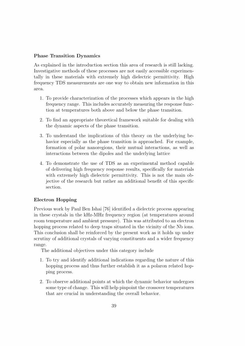
Phase Transition Dynamics
As explained in the introduction section this area of research is still lacking.Investigative methods of these processes are not easily accessible experimen-tally in these materials with extremely high dielectric permittivity. Highfrequency TDS measurements are one way to obtain new information in thisarea.
1. To provide characterization of the processes which appears in the highfrequency range. This includes accurately measuring the response func-tion at temperatures both above and below the phase transition.
2. To find an appropriate theoretical framework suitable for dealing withthe dynamic aspects of the phase transition.
3. To understand the implications of this theory on the underlying be-havior especially as the phase transition is approached. For example,formation of polar nanoregions, their mutual interactions, as well asinteractions between the dipoles and the underlying lattice
4. To demonstrate the use of TDS as an experimental method capableof delivering high frequency response results, specifically for materialswith extremely high dielectric permittivity. This is not the main ob-jective of the research but rather an additional benefit of this specificsection.
Electron Hopping
Previous work by Paul Ben Ishai [76] identified a dielectric process appearingin these crystals in the kHz-MHz frequency region (at temperatures aroundroom temperature and ambient pressure). This was attributed to an electronhopping process related to deep traps situated in the vicinity of the Nb ions.This conclusion shall be reinforced by the present work as it holds up underscrutiny of additional crystals of varying constituents and a wider frequencyrange.
The additional objectives under this category include
1. To try and identify additional indications regarding the nature of thishopping process and thus further establish it as a polaron related hop-ping process.
2. To observe additional points at which the dynamic behavior undergoessome type of change. This will help pinpoint the crossover temperaturesthat are crucial in understanding the overall behavior.
39

3. To investigate this process as it crosses over from the paraelectric phaseto the ferroelectric. This requires measurements at very low frequen-cies.
4. To investigate the effects of pressure on this process. The point isto see if it affects the relaxation times and/or the dielectric strengthand shape of the process. This will provide important clues as to theinteractions and correlations between the relaxing entities.
Dipole-Lattice Interactions and Dipole Correlation Length
The theoretical framework establishing the connection between the dielectricmeasurements and the dipole-lattice interactions has been introduced andshown to stem from the works of Ryabov and later adaptations of Ben Ishai[76] In this work we further explore the connection to the Burns temperature,the low temperature (low frequency) behavior as the dielectric process crossesthe phase transition, and finally the effects of pressure on these interactions
The additional objectives under this category include
1. To develop a theoretical framework suitable for dealing with transientdipoles, allowing us to gain insight into system containing hoppingprocesses.
2. To integrate this theory with our experimental findings and apply itto derive useful information regarding the structure or dynamics of theunderlying lattice.
1.7.3 Experimental Goals
Achieving the above goals requires a comprehensive study of the dielectricproperties of a specific KTN crystal, beyond what was perviously done. Thismeans covering a very wide frequency range and will therefore include varyingthe following parameters:
1. Frequency variation in the high frequency range 106 Hz to 109 Hz per-formed via TDS.
2. Frequency variation in the mid frequency range 10−2 Hz to 107 Hzperformed via BDS.
3. Variation of temperature at all frequencies.
4. Variation of Pressure 0-7.5kbar at mid frequency range.
40

1.7.4 Impact
There are two reasons why studies of this nature are very important.
1. The first is on the level of basic science. There is much insight to begleamed from a thorough investigation of these crystals and their prop-erties. Although much has already been uncovered and many bookseven devoted to the subject [2, 20, 22] advances in technology alwaysinevitably lead to better precision measurements opening up the doorfor discovering ever more fascinating details. The scope and accuracy ofdielectric measurements performed nowadays is obviously much morecomprehensive illuminating areas which were previously inaccessible.
2. The second is on the level of applied science. If we want to fully ex-ploit the technological potential of these materials we must first fullyunderstand all of their advantages and limitations in order to properlydecide where and when they can be used best. Of particular interestare the impurity behaviors themselves. Being the focus of a disturbancein the crystal lattice they are expected to exhibit relaxation behaviorwhen subject to an external impetus, such as an electric field. Howtheir local environment, particularly when passing through the phasetransition, will modify this behavior is of importance when consider-ing practical applications based on them. All real time application arenecessarily dependent on a time window, thereby emphasizing a needfor a thorough knowledge of all processes occurring at the relevant timescales.
Achieving these goals requires a focused and methodological approach tothe investigations. We must clearly define what exactly we intend to measure,what parameters will we be playing with and monitoring their effect andfinally what is the meaning of each parameter and what underlying realitydoes it mirror in on microscopic level.
41

42

Chapter 2
Materials & Methods
2.1 Crystal Preparation
2.1.1 Crystal Growth
A series of KTN crystals was prepared with varying levels of Niobium,Lithium and Copper in the melt. For the present study the most importantparameter was the Niobium level as we mainly focused specifically on the Nbrelated processes as will be discussed. In any case all the KTN crystals underinvestigation The crystals were grown by the Crystal Growth Laboratory ofProf. A.J. Agranat, using the top seeded solution growth method [34]. Moreinformation on this method along with detailed explanations can be foundin Reference [77]. An enlarged image is shown in figure 2.1.
The Ta/Nb ratio was estimated by electron microprobe analysis or by thephase transition temperature. In all crystals an attempt was made to keep
Figure 2.1: Picture of crystal as it appears right after being grown.
43

Figure 2.2: Dependance of Phase transition temperature on Ta/Nb concen-tration. Taken from [78].
the Ta/Nb ratio at similar levels in order to guarantee a phase transition atroom temperatures. Estimation of this Ta/Nb was done by interpolation,taking the ferroelectric phase transition temperature and finding where itfalls on the plot vs. Nb concentration. As in our previous work [76] thelinear equation T c ∼ 682∗Nbconc(%)+33.2, was used to approximate the Nbconcentration as shown in the plot in figure 2.2. Generally the Ta/Nb wasfound to be in the vicinity of 62/38 per mole giving a transition temperatureright in the desired area of 300 Kelvin. One KTN crystal containing only21% Niobium per mole was measured in previous studies [76] in order togauge the effect of Nb concentration on the observed behaviors. This crystalof course had a much lower Phase Transition temperature.
Many of the crystals contained a small amount of additional disorderin the form of Cu or Li impurities. A pure KTN crystal was prepared asreference. For crystals doped with Copper the doping level was 2% in theflux yielding approximately 1.5×10⁻⁴ per mole in the grown crystal. Thelatter estimate was verified in similar crystals by measurements of the Cuconcentration in the grown crystal using Inductively Coupled Plasma MassSpectrometry [76]. The full set of crystal compositions and parameters, re-lating to any of the crystals mentioned in this study, are listed in the nextsection.
Samples of approx. 1x1x2 mm3 were cut from the grown bole along the
44

Table 2.1: KTN/KLTN crystals specifically focused on in this study, withvarying copper content.
Crystalno.
Constituents CuCon-tent%
LiCon-tent%
Pure KTa0.62Nb0.38O3 0 0100 KTa0.65Nb0.35O3 : Cu 1.2 0120 KTa0.62Nb0.38O3 : Cu 2.0 09038 K0.972L0.028Ta0.63Nb0.37O3 :
Cu3.5 3.5
crystallographic [001] axes. The x-y faces of the sample (perpendicular to thegrowth direction z) were polished and coated with gold electrodes. Figure2.1 shows a picture of a samples as it appears just prior to the measurements.
2.1.2 Crystal Composition
The full set of crystals used both in this investigation and in the previousinvestigations leading up to it are listed in the two tables. From within thisbroader set the investigation actually focused on two specific crystals, onepure KTN (labeled ’Pure’) with no Cu added, and one with a small amountof Cu (crystal 120). The former was used to investigate the dynamics of thephase transition itself, specifically the role of Nb polar nanoregions within it.The latter was used for a wider scope of interactions sometimes taking intoaccount the additional disorder induced by the Cu defects. The content ofCu was about 2% in the melt, leading as noted above to about 0.00015 moleconcentration in the crystal. In crystal 100 the Cu content in the melt wasonly 1.2% by weight leaving an even lower impact on the fully grown crystal.
The crystals used in this study have a high Niobium concentration ( 38%)so they should behave as a classic ferroelectrics with 2nd order displacive tran-sitions. However, some features of relaxor behavior do remain. In a classicalferroelectric there is no macroscopic polarization above the transition tem-perature. The Burns temperature signifies the onset of clusterization of thepolarizable ions in the lattice leading to polar nanoregions. It is correlationsbetween these dipolar entities that lead to the relaxor behavior, including afrequency dependent ferroelectric phase transition temperature and a devia-tion from Curie Weiss.
45

Table 2.2: KTN/KLTN crystals from previous studies (mentioned here aswell) prepared with varying Lithium and/or copper content.
Crystalno.
Constituents CuCon-tent%
LiCon-tent%
083 K0.972Li0.028Ta0.62Nb0.38O3 :Cu
2.0 8
077 K0.976Li0.024Ta0.62Nb0.38O3 0 4R128 KTa0.79Nb0.21O3 0 0
Figure 2.3: Equivalent electronic circuit of simple lumped capacitance.
2.2 Frequency Domain Measurements
2.2.1 Spectrum Analyzer
For the frequency range used in this study a sample sandwiched betweentwo parallel plates and subjected to a constant field can be considered as alumped element. Its impedance can be modeled by a simple equivalent cir-cuit, whereby C models the capacitive behavior of the sample and R modelsconductive losses in the sample.
The impedance of the circuit is given by
1
Z(ω)=
1
ZC (ω)+
1
ZR (ω), (2.1)
Inverting the equation we derive the expression for the complex permittiv-ity, ǫ∗(ω), in the lumped capacitance approximation where σdc is the conduc-tivity of the sample. Separating the permittivity into its real and imaginary
46

Figure 2.4: The schematic for the inclusion of an electrometer and referencecapacitors in the active head of the dielectric analyzer. A low current opera-tional amplifier is included for frequencies less than 100 kHz, allowing currentmeasurements as sensitive as 1 fA.
components we have
ε′ =−Z ′′
ωC0 |Z|2. (2.2)
ε′′ =Z ′
ωC0 |Z|2+σdcωε0
(2.3)
For non conductive samples the dielectric losses are characterized by theloss angle δ:
tan (δ) =ε′′
ε′=
Z ′
−Z ′′ (2.4)
There are a number of methodologies to measure the complex impedance[11]. The method involved in this study is explained in the next section.
The system used for the dielectric measurements was an Alpha HighResolution Dielectric Analyzer with a Cryogenic temperature control systembased on liquid Nitrogen. The entire turnkey system is supplied by Novo-control GmbH, Hundsangen Germany.
The analyzer consists of two parts: A frequency response analyzer witha sine wave and dc generator and two ac input channels. Each channelmeasures the ac voltage amplitude of the applied sine wave. The phase shiftbetween the two is also detected. The second part is an impedance convertera wide dynamic current to voltage converter and a set of precision referencecapacitors. These are incorporated into the cell holder directly, allowingprecise calibration of artifact resulting from the cell itself. This leads to avery accurate measurement of the sample impedance with errors in tan(δ) ofless than 10−4.
47

The principles of the dielectric measurement are simple and illustrated inFigure 2.4. A voltage U0 with a fixed frequency is applied to the cell, causinga current I0 to flow with the same frequency but with a phase difference ofϕ, which depends on the nature of the sample.
U(t) = Re(U0eiωt), I(t) = Re(I∗eiωt), (2.5)
where
I∗ = I ′ + iI ′′ ; I0 =√I ′2 + I ′′2 ; tan(ϕ) =
I ′′
I ′. (2.6)
The complex impedance of the sample is
Z∗(ω) = Z ′ + iZ ′′ =U0
I∗=
U0
I0(cosϕ − i sinϕ)
∣∣∣∣ω
. (2.7)
When the response of the sample is linear the relationship to the complexpermittivity is given by
ε∗(ω) = ε′(ω)− iε”(ω) =1
iωC0ε0
1
Z∗(ω). (2.8)
where C0 is the geometric capacitance of the sample. The resulting expressionis:
ε∗(ω) = ε′(ω)− iε′′(ω) =I0
iωC0U0
(cosϕ+ i sinϕ)
∣∣∣∣ω
(2.9)
The accuracy of the dielectric measurement is improved by the inclusion ofan active head between the sample and the analyzer. This head containsa broadband electrometer, an amplifier with a variable gain and variablecapacitors. The schematic is shown in Figure 2.5. If the variable impedance,changed in resistance and capacitance, is denoted by Z∗
X(ω), then the sampleimpedance, Zs(ω) of a direct measurement is given by:
Z∗s (ω) =
U∗1S (ω)
I∗S (ω)= −U
∗1S (ω)
U∗2S (ω)
Z∗X (ω) (2.10)
If the reference capacitors are accurately known then inconsistencies in theelectrometer can be eliminated giving
Z∗s (ω) =
U∗1S (ω)
U∗2S (ω)
· U∗2R (ω)
U∗1R (ω)
Z∗R (ω) (2.11)
where Z∗R(ω) is the impedance of the accurately known reference capacitors.
Using this methodology it is possible to obtain accuracies of 10−4 intan(δ). However, for such accuracies the sample capacitance cannot stray
48
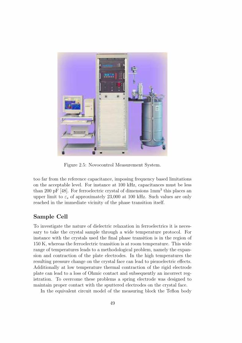
Figure 2.5: Novocontrol Measurement System.
too far from the reference capacitance, imposing frequency based limitationson the acceptable level. For instance at 100 kHz, capacitances must be lessthan 200 pF [48]. For ferroelectric crystal of dimensions 1mm3 this places anupper limit to εs of approximately 23,000 at 100 kHz. Such values are onlyreached in the immediate vicinity of the phase transition itself.
Sample Cell
To investigate the nature of dielectric relaxation in ferroelectrics it is neces-sary to take the crystal sample through a wide temperature protocol. Forinstance with the crystals used the final phase transition is in the region of150 K, whereas the ferroelectric transition is at room temperature. This widerange of temperatures leads to a methodological problem, namely the expan-sion and contraction of the plate electrodes. In the high temperatures theresulting pressure change on the crystal face can lead to piezoelectric effects.Additionally at low temperature thermal contraction of the rigid electrodeplate can lead to a loss of Ohmic contact and subsequently an incorrect reg-istration. To overcome these problems a spring electrode was designed tomaintain proper contact with the sputtered electrodes on the crystal face.
In the equivalent circuit model of the measuring block the Teflon body
49

Figure 2.6: Sample cell used for dielectric measurements of pressure sensitivecrystals.
will appear as a parallel parasitic capacitance. As the high frequency, hightemperature limit of the crystal permittivity is at least 2 orders of magnitudegreater than the dielectric constant of Teflon this parasitic capacitance isnegligible. The inductance introduced by the spring to the total impedancewas estimated using the expression of a circular loop as a first approximation.
L = rµ0µr
(ln
(8r
a
)− 2
), (2.12)
where r is the radius of the loop, a is the radius of the conductor, µ0 is thepermeability of free space and µr is the relative permeability of the medium.If the conducting strip is considered as a series of identical inductances inparallel then
L =
(N∑
i=1
1
Li
)−1
=rµ0µr
w/a
(ln
(8r
a
)− 2
), (2.13)
where w is the width of the strip, a is the thickness and µr= 1. For theconstructed sample holder r = 5 ± 0.1mm. Coupled to the capacitance ofthe crystal this leads to a parasitic resonance in the signal with frequency
ωr = 1
/√LC = c
/√rεrA
dw/a
(ln
(8r
a
)− 2
), (2.14)
where A is the area of the crystal face, d is the crystal thickness and c =1/√
µ0ε0 is the speed of light. The crystal dimensions where A= 1mm2 andd=1mm. The calculated resonance for the range of crystal permittivitiesexperienced was 108Hz < ω < 1010Hz, far outside the measurement windowused.
50

Temperature Protocol
Measurements were generally performed primarily in the Paraelectric phase.The crystals were first heated to at least 50 degrees above the phase transitionand then measured upon cooling. The typical temperature step was about 5degrees, except in the immediate vicinity of the PT where the sensitivity wasincreased to steps of 1 degree. Temperature stabilization was kept within0.2K and the samples were held at the temperature point for 60 seconds forthermal stabilization before measurement initiation.
Low Frequency Measurements
One crystal (labeled 9038 above) was also measured at the very low frequencyend of the machine capabilities going down all the way to 10−4Hz for a fewselect temperatures in the vicinity of the phase transition where some of thedynamics are very slow.
The measurement technique was basically the same. Only the main differ-ence now, was that due to the extended duration of the measurement accuratetemperature stabilization becomes of paramount importance. The tempera-ture was therefore kept stable to within 0.1K for these measurements. Alsothe 60 second stabilization prior to measurement initiation was increased to600 seconds to ensure the stabilization throughout the entire measurementduration.
2.2.2 Data Treatment
Dielectric relaxation of complex materials over wide frequency/time and tem-perature ranges may be described in terms of several distributed relaxationprocesses. A quantitative analysis of the dielectric spectra begins with theconstruction of a fitting function in selected frequency/time and temperatureintervals, which corresponds to the relaxation processes in the spectra. Thisfitting function is a linear superposition of the model functions (such as CC,CD, and HN mentioned above) that describe the frequency or time depen-dence of the isothermal data of the complex dielectric relaxation. However,there are several problems in selecting the proper fitting function, such as thelimited frequency/time and temperature ranges of the experiment, distortioninfluences of the sample holder and the overlapping of several physical pro-cesses with different amplitudes in the same frequency/time and temperatureranges. The latter is the most crucial problem, because some of the relaxationprocesses can simply be screened by the others. For such a screened process,the confidence in parameter estimations may be very small. In this case,
51
the functional temperature behavior of the parameters may be inconsistent.Despite these discontinuities, there may still be some trends in the parame-ter behavior of the screened processes, which may reflect some tendencies ofthe physical processes in the system. Therefore, it is desirable to obtain acontinuous solution of the model parameters via temperature. This solutionis hardly achievable if the estimation of the parameters is performed inde-pendently for the different temperature points on the selected fitted range.Post-fitted parameter smoothing can spoil the quality of the fit.
Often the presence of dc conductivity can make it difficult to analyzerelaxation processes, especially when the contribution of the conductivity ismuch greater than the amplitude of the process. In such cases the correctcalculation of the dc conductivity is vital in terms of the subsequent analysisof the dielectric data. Its evaluation by fitting of the experimental data doesnot always give correct results, especially when strong relaxation processesare present in the low frequency range. Fortunately for our purposes inthe case of Ferroelectric crystals this in not the case and we may proceedusing the normal analysis techniques. As the temperature is increased muchabove the PT these effect become much more dominant requiring specialmethods of analysis and deconvolution. In particular, the dc conductivityfunction has frequency power-law dependence similar to the Jonscher termsin the imaginary part of the complex dielectric permittivity and this makescomputation of dc-conductivity even more difficult.
The main take away point is therefore that the dielectric spectroscopydata analysis is thus be reduced to the problem of choosing the appropriatemodel functions and an estimation of their model parameters. Software fordielectric data treatment and modeling in frequency domain has been de-veloped recently [79]. This program (DATAMA) was built around the soft-ware package MATLAB (Math Works Inc.) and its functionality is availablethrough an intuitive visual interface. Key features of the program include:
1. Advanced data visualization and pre-processing tools for displayingcomplex dielectric permittivity data and selecting appropriate frequencyand temperature intervals for modeling;
2. A library of standard relaxation fit functions;
3. Simultaneous fit of both real and imaginary components of the complexdielectric permittivity data;
4. Linear and nonlinear fitting methods, from least-squares and logarith-mic to fitting procedures based on the entropy norm;
52
5. Global fit procedure on all selected temperature ranges for continuousparameter estimation;
6. Hilbert transform for computing dc conductivity;
7. Parameter visualization tool for displaying fitting parameter functionsvia temperature and subsequent analysis of the graphs.
The methodology described above, utilized in the presented program [79],and reduces the problem of dielectric data analysis to choosing the appro-priate model functions and an estimation of their model parameters. Thepenalized maximum likelihood approach for obtaining these parameters as afunction of temperature has proven to be a consistent method for accuratelyobtaining the global minimum in this estimation. This methodology is aphenomenological approach to obtaining the underlying temperature depen-dence of the parameter space, while not presupposing a particular physicalmodel. The risk is present that such a regularization routine may perturbthe result if used excessively. For this reason a regularization parameter isused to control the smoothing term. However, this risk is far less than therisk of a priori conclusion of the result according to the researcher’s personalbelief in a preferred analytical model.
2.3 Time Domain Measurements
The standard Frequency domain method employed for performing dielectricmeasurements at high frequencies (10MHz-10GHz) uses RF impedance ana-lyzers based on coaxial line reflectometry. This method is not suitable whendealing with materials exhibiting extremely large values of dielectric permit-tivity. In ferroelectric crystals for example the value of ε′ is often tens ofthousands. As such they cannot be measured accurately using standard fre-quency based methods. For materials where ε′ is only a few thousand somemeasurements can be made up to 1GHz using specially designed sample cells.The Time domain spectroscopy(TDS) method was specifically chosen in or-der to avoid the experimental errors occurring in the frequency domain. Theaccuracy of the time domain measurements is determined primarily by thesignal-to-noise ratio. Typical systems my have error values of up to 5%. Thephase shift in frequency domain actually works to our advantage when mea-suring in the time domain. It corresponds to a time shift thus increasing thesignal accuracy by reducing the errors coming from the time shift betweenthe signal reflected from the sample and the calibrated reference standard.
53
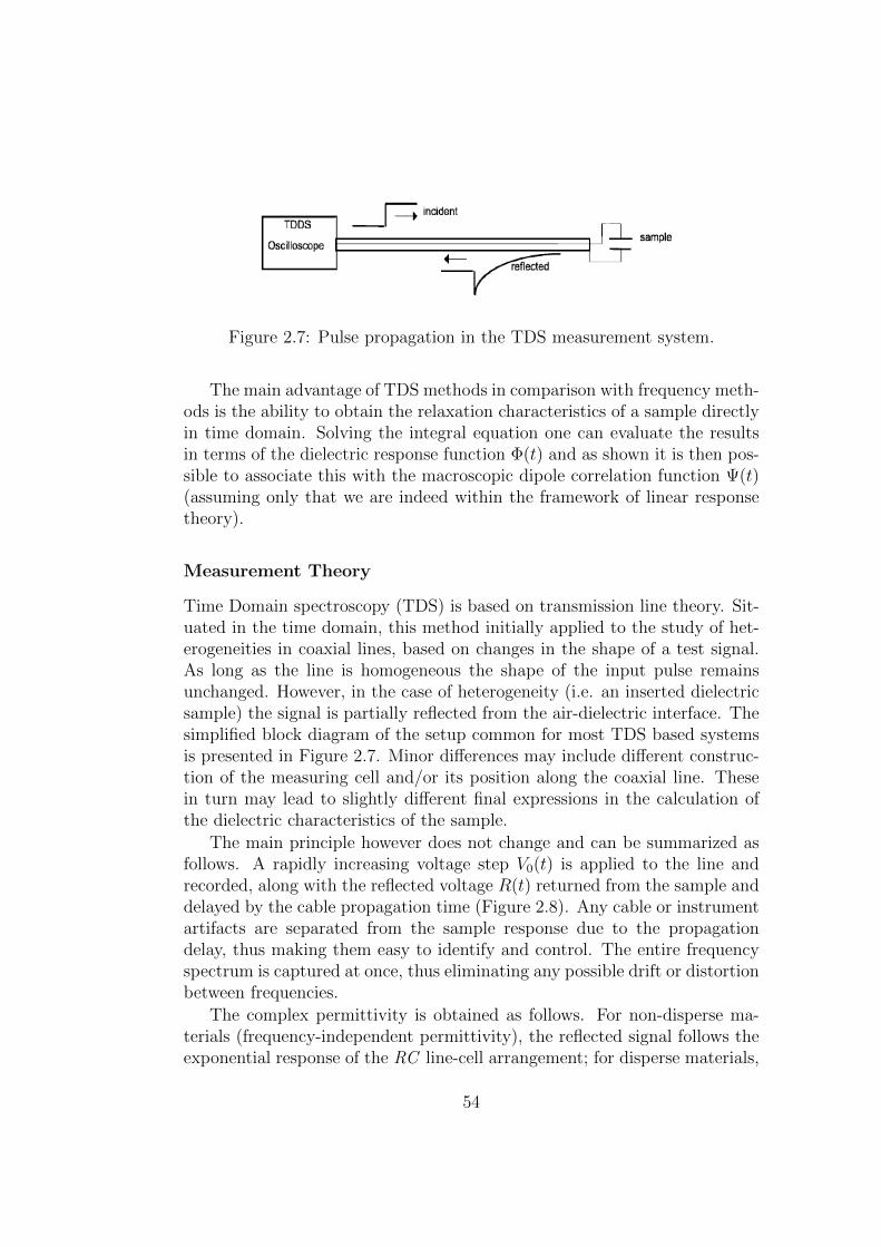
Figure 2.7: Pulse propagation in the TDS measurement system.
The main advantage of TDS methods in comparison with frequency meth-ods is the ability to obtain the relaxation characteristics of a sample directlyin time domain. Solving the integral equation one can evaluate the resultsin terms of the dielectric response function Φ(t) and as shown it is then pos-sible to associate this with the macroscopic dipole correlation function Ψ(t)(assuming only that we are indeed within the framework of linear responsetheory).
Measurement Theory
Time Domain spectroscopy (TDS) is based on transmission line theory. Sit-uated in the time domain, this method initially applied to the study of het-erogeneities in coaxial lines, based on changes in the shape of a test signal.As long as the line is homogeneous the shape of the input pulse remainsunchanged. However, in the case of heterogeneity (i.e. an inserted dielectricsample) the signal is partially reflected from the air-dielectric interface. Thesimplified block diagram of the setup common for most TDS based systemsis presented in Figure 2.7. Minor differences may include different construc-tion of the measuring cell and/or its position along the coaxial line. Thesein turn may lead to slightly different final expressions in the calculation ofthe dielectric characteristics of the sample.
The main principle however does not change and can be summarized asfollows. A rapidly increasing voltage step V0(t) is applied to the line andrecorded, along with the reflected voltage R(t) returned from the sample anddelayed by the cable propagation time (Figure 2.8). Any cable or instrumentartifacts are separated from the sample response due to the propagationdelay, thus making them easy to identify and control. The entire frequencyspectrum is captured at once, thus eliminating any possible drift or distortionbetween frequencies.
The complex permittivity is obtained as follows. For non-disperse ma-terials (frequency-independent permittivity), the reflected signal follows theexponential response of the RC line-cell arrangement; for disperse materials,
54

Figure 2.8: Input and Reflected TDS signals.
the signal follows a convolution of the line-cell response with the frequencyresponse of the sample. The actual sample response is found by writing thetotal voltage across the sample as follows
V (t) = V0(t) +R(t). (2.15)
and the total current through the sample
I(t) =1
Z0
[V0(t)−R(t)]. (2.16)
where the sign change indicates direction and Z0 is the characteristic lineimpedance. The total current through a conducting dielectric is composed ofthe displacement current ID(t), and the low-frequency current between thecapacitor electrodes IR(t). Taking the active resistance at zero frequency ofthe sample-containing cell to be:
r = limV (t)
I(t)= Z0 lim
V0(t) +R(t)
V0(t)−R(t). (2.17)
this low-frequency current can be expressed as:
IR(t) =V (t)
r=V0(t) +R(t)
Z0
limV0(t)−R(t)
V0(t) +R(t). (2.18)
Relation (2.16) can now be written as:
ID(t) =1
Z0
[V0(t)−R(t)]− [V0(t) +R(t)] limV0(t)−R(t)
V0(t) +R(t). (2.19)
Relations (2.15) and (2.19) present the basic equations which relate I(t)and V (t) with the signals recorded during the experiment. In addition, (2.19)shows that TDS permits one to determine the low-frequency conductivity σof the sample directly in time domain:
σ =ε0
Z0C0
limV0(t)−R(t)
V0(t) +R(t). (2.20)
55

Using I(t), V (t) or their complex Fourier transforms i(ω) and v(ω) wecan once again accurately map the relations describing the dielectric charac-teristics, moving back and forth between frequency and time domain. Theexact form of these relations depends of course on the precise geometric con-figuration of the sample cell and its equivalent electrical representation.
The admittance of the sample cell terminated to the coaxial line is thengiven by
Y (ω) =i(ω)
v(ω)(2.21)
and the sample permittivity may be presented as follows:
ε(ω) =Y (ω)
iωC0)(2.22)
In order to minimize the effect of line artifacts and also establish a clearcommon time reference, (2.21) is usually rewritten in differential form, tocompare reflected signals from the sample and a calibrated reference standardand thus eliminate V 0(t).
If one takes into account the definite physical length of the sample andmultiple reflections from the air-dielectric or dielectric-air interfaces, relation(2.22) must be written in the following form:
ε∗(ω) =c
iω(γd)Y (ω)X cotX (2.23)
where d is the length of the inner conductor, c is the velocity of light, andγ is the ratio between the capacitance per unit length of the cell to thatof the matched coaxial cable. Equation (2.23) in contrast to (2.22) is atranscendental one, and its exact solution can be obtained only numerically.
2.3.1 Measurement Apparatus
Dielectric measurements were performed in the time domain using the TDSmethod. This method was chosen in order to avoid the experimental errorsoccurring in the frequency domain when dealing with extremely large valuesof the static dielectric constant. The system used was a TDS-2 (Dipole) set-up consisting of a signal recorder, a sampler and a built in pulse generator.The shape of the reference voltage pulse and the response of the samplewere digitized and averaged by the digitizing block of the Time DomainMeasurement System. A detailed description of the system and the theorybehind it can be found in reviews in the scientific literature [80].
The typical TDS set-up consists of a signal recorder, a 2-channel samplerand a built-in pulse generator. The generator produces 200mV pulses of 10µs
56

Figure 2.9: TDS measurement system.
duration and short rise time (∼ 30 ps). Two sampler channels are character-ized by an 18GHz bandwidth and 1.5 mV noise (RMS). Both channels aretriggered by one common sampling generator that provides their time cor-respondence during operation. These were indeed the very parameters usedin our system. The time base is responsible for the major metrology TDMSparameters. The block diagram of the described TDS set-up is presented inFigure 2.9.
In highly disordered complex materials, the reflected signal R(t) mayextend over wide ranges of time thus preventing the possibility of capturingall the data on a single time scale with adequate resolution and samplingrate. In an important modification of regular TDR systems, a nonuniformsampling technique, has been employed.
The structure of the time scale allows the overlapping of the time rangefrom 5ps to 10µs during one measurement, which results in a limited numberof registered readings. The overlapped range can be shortened, decreasingthe number of registered points thus reducing the time required for datarecording and processing.
The major advantage of the multi-window time scale is the ability to getmore comprehensive information. The signals received by using such a scalecontain information within a very wide time range and the user merely de-
57

Figure 2.10: Sample cell used for TDS measurements of KTN crystals, bulkcapacitance configuration.
cides which portion of this information to use for further data processing.Also, this scale provides filtration of the registered signals at close to the op-timal level approaching the level already employed at the stage of recording.
Sample Cell
The sample cell was an ordinary plate capacitor terminated to the centralelectrode on the end of the coaxial line. The sample was inserted and sat onthis central electrode. Due to the extremely large values of the permittivityfringing field effect could be easily neglected. care was taken not to applyexcessive pressure on the sample when terminating the circuit so as not toinclude unwanted effects.
Temperature Protocol
Temperature of the sample cell was controlled by a Julabo F10 circulatoryheat bath. Temperature range of the TDS measurements was from 270-360K. Temperature jumps were in steps of 5-10K except in the vicinity ofthe phase transition where smaller steps were taken. The estimated accuracyin the temperature stabilization was better than 0.2K.
58

Figure 2.11: Snapshot of the TDS sample cell.
2.3.2 Data Treatment
The software used for the time domain analysis was also a home developedwindows based program. It was heavily reliant on graphical interface dueto the fact that accurate assessment of the signal shape including the longtime behavior is critical for obtaining the correct treatment. Each sample’streatment is quite individual, requiring its own devoted attention, somethingwhich renders simple automatic batch processing difficult and somewhat un-reliable. Recently improvement have been made to the program which doallow a great deal of automation but this was unfortunately not the case atthe time when our measurements were performed.
The software is capable of producing both the Dielectric Spectra and theResponse function independently of one another. The charge buildup overthe sample and the sample conductivity can be calculated and saved for lateranalysis. While the main scheme is the Lumped Capacitance Approximationan iteration procedure may be included to take the user up to the maximumtheoretical frequency limit.
For our purposes we were more interested in the dipole correlation func-tions which as explained relate directly to the time response functions. Forthis reason we were mainly interested in the analysis directly in the timedomain. The percolation based theoretical model was developed for the timedomain and the subsequent interpretations that it provides relate to these
59
time dependant parameters. Therefore it was only natural that the dataanalysis of the percolation process for the studied systems should be doneusing the time domain data provided in terms of the DCF.
2.4 Pressure Measurements
Applying pressure can be done in a number of different ways with vastlydifferent outcomes. The main parameters that must be controlled are thelevel of the pressure applied and the direction (hydrostatic vs. directional).Pressure measurements were performed only in the frequency domain. Ingeneral, the pressure measurements did not differ in principle from the pre-vious measurements and are based on the same theoretical principles. Themain difference is of course the special apparatus needed in order to carryout the above measurement while applying the hydrostatic pressure. In ourlaboratory we did not have access to the necessary equipment and insteadthese measurements were performed in the laboratory of Dr. Marian Paluchin Poland and in collaboration with his research group.
2.4.1 Measurement Apparatus
Measurement of the dielectric properties in the frequency domain were per-formed with an almost identical Novocontrol system. The pressure measure-ments used either oil (0-5kbar) or gaseous helium (7.5kbar) as the hydro-static pressure transmitting media. Two apparatus were used: a pressurecell charged from a compressor/intensifier system and a large-volume pis-ton/cylinder apparatus. Calibrated gauges were used to measure the pres-sure. Dielectric measurements were carried out in a frequency range from10−1 to 107 Hz using the same model Novocontrol Alpha Impedance Ana-lyzer. The sample was placed in a Teflon bellows filled with the silicon oiland mounted in the high-pressure chamber. Displacing the piston by meansof a hydraulic press generated the hydrostatic pressure.
2.4.2 Sample Cell, Temperature Protocol and DataTreatment
For the pressure measurements we were unable to use the spring designsample holder, consequently temperature regime was reduced. At the iso-baric conditions, the measurement was carried out and the temperature waschanged within the 270-360K range, with a step of 5K [81].
60

Figure 2.12: Measurement system for combined Dielectric measurementsalong with hydrostatic pressure application.
Data treatment was identical to the standard broadband dielectric anal-ysis described above. The addition of pressure does not interfere with thispart of the analysis in any way.
61

62

Chapter 3
Results and Discussion
Taking into account that the results were obtained using a number of com-plimentary experimental setups and cover a broad range of topics, their pre-sentation and analysis follows on the same scheme in which the investigationwas performed. As each new set of results is introduced it is immediatelyfollowed by the relevant discussion and analysis pertaining to that particularset.
For reasons of clarity the previous sections began with the description ofthe frequency domain methods. Nevertheless we shall start here with thehigher frequency results obtained in the time-domain measurements. Theserelate more directly to the faster processes concerning the phase transitionand Niobium ions themselves. This is important to establish first as it relatesto the global macroscopic properties of the material. Once the underlyinglattice behavior has been successfully determined, we can then turn to thelower end of the spectrum, utilizing the frequency domain results. Theseshall be shown to relate to an electron hopping process independent of thephase transition.
Despite its independence, results will show that some of the parametersrelating to this hopping process are nevertheless indirectly affected by thephase transition. This comes about due to the changes manifest in the un-derlying landscape upon which the hopping takes place, as it is radicallytransformed. Finally, the pressure investigations will give us yet anotherwindow into exploring this relation between the hopping process and under-lying lattice. Changing the pressure allows us a certain measure of controlover the landscape thereby providing a way to change this interaction andtest it under different conditions.
Analysis of each set of results was done independently, focused on differentfrequency bands and thus inevitably relate to different processes going onsimultaneously at different scales. This is outlined in three parts as follows:
63

1. First the results obtained in the time domain measurements. Theseresults relate, as will be shown, to the Phase transition dynamics. Theycorrespond specifically to the Nb ions inside the crystal lattice andshould be intrinsic to any KTN crystal regardless of its constitution. Ofcourse, the constitution will effect the values of the parameters but notthe qualitative behavior, unless the lattice is drastically altered to thepoint where the phase transition is somehow suppressed or inhibited.
2. Next the frequency domain results are presented. These results willbe shown to correspond to an electron hopping, polaron related pro-cess. Parameters of this relaxation process will provide insight intothese hopping dynamics in the crystal and how it is affected by thephase transition. This process will be shown to be universal for all Nbconcentrations and independent of any Li or Cu defects.
3. Finally the results of the frequency domain measurements under pres-sure. This comes after having identified the electron hopping processin the previous section. Using the knowledge obtained as an initialunderstanding of the relaxation parameters we reapply them here inorder to see what they can tell us about the system. This section thenserves to deepen our understanding of these parameters and gain addi-tional insights into the electron hopping process and how the pressurechanges and affects the landscape.
3.1 Time Domain Results -
Phase Transition Dynamics
3.1.1 Time Domain Results
Response Functions
In the time domain the results presented here all pertain to Crystal 100(Table 2.1 above) upon which the extensive analysis in the time domain wasperformed. This crystal contained only trace amounts of Cu and thereforeall of the dynamics should relate in some way to the Nb ions. As will beshown later, even in the frequency domain measurements where the Cu hasbeen shown to manifest as a relaxation process no such process was noted inthis crystal.
Additional crystals were measured with varying levels of Cu, howevertheir landscape in the corresponding frequency range was much more com-plex. There are a number of additional processes going on at these frequencies
64

Figure 3.1: Response functions measured in the time domain at differenttemperatures. As the phase transition is approached the amplitude of theresponse is seen to increase.
related to the additional defects inside the lattice. These processes screen outthe Nb process making it much more difficult to analyze and characterize.There is much room for additional analysis in this direction but it proved toocomplicated for the current study. This behavior has yet to be independentlyconfirmed in another crystal with different constituents and this point shouldbe addressed in further studies.
Results of the time domain measurements are presented in terms of theresponse functions and can be seen in figure 3.1. Combining the slices into athree dimensional plot produces figure 3.2.
Dielectric Landscape
Converting the response function via Fourier Transform into the frequencydomain dielectric function is relatively straight forward. Its purpose here isonly secondary, to get a picture of how it will look, as our analysis will beapplied directly in the time domain. Nevertheless if we wanted to we couldapply the frequency based analysis to the results in the same fashion as willbe done to the results obtained directly in the frequency domain.
In this case however, we felt there was more information to be obtained inthe time domain analysis. The signal is also a bit less noisy as it has not gone
65

Figure 3.2: Three dimensional plot of the response functions with both timeand temperature dependance. The phase transition is clearly evident as is thefact that the shape of the response function changes as well as the transitionis approached.
through the fourier transform. Furthermore we don’t have to worry aboutcutoff issues and other artifacts which can appear during the transformationprocess. Nevertheless, in order to get a feeling of what the process looks likeand where it stands in relation to the frequency domain measurements ofthe following section. Figures 3.3 and 3.4 present the actual picture obtainedfrom the Fourier Transform and showing the process in the frequency domain.
Relaxation Strength
Of the five relaxation parameters which appear in equation (1.48), four wereused to fit the results (τ1 was found to be nearly constant and thus set ata fixed value, for this reason we shall also refer to τM simply as τ). Theyare presented in Figure 3.5(a-d) each one in its own quadrant. Two verticaldotted lines are inserted into each figure marking the phase transition pointas well as the intermediate temperature both of which will be important lateron in the analysis.
The prefactor A is actually directly related to the relaxation strength∆ε [46] and is for the most part predictable obeying the well established
66

Figure 3.3: Dielectric response in the frequency domain. Results obtainvia simple Fourier Transform of the data in the previous graphs. The realcomponent of the complex dielectric constant ε∗.
Curie-Weiss dependance (Figure 3.5(a)). There is a region close to the phasetransition where the values begin to deviate from this dependence. Thisbehavior is also well known and well established, but it does give us anindication as to where the Burns temperature may be found [82].
Relaxation Times
The relaxation times are shown in figure 3.5(b). In the high temperaturesthe behavior is Arrhenius as expected with a clearly definable Activationenergy (∆E ∼ 1.0meV ). Slightly above the phase transition (about 20 de-grees) the relaxation starts to change as it starts to disproportionately slowdown, showing interesting behavior in deviating from the standard Arrheniusdependence. This will be further explored in the discussion.
Behavior below the Phase transition in the Ferroelectric phase is alsointeresting. The relaxation actually speeds up before slowing down onceagain. Based on the shape of the curve it indicates a type of confinementprocess as discussed at length in reference [76]. We shall not go into in depthanalysis of this behavior here.
67

Figure 3.4: Dielectric response in the frequency domain. Results obtain viasimple Fourier Transform of the data in the previous graphs. The imaginarycomponent of the complex dielectric constant ε∗.
Power and Stretch Parameters
The power and stretch parameters µ and ν (which relate to the percolation,and the statistical cluster distribution) are shown in figure 3.5(c) and 3.5(d).Their behavior contains information on the growth and distribution functionsof the polar clusters as shall be discussed.
The behavior of all of these parameters indicates that we are indeed see-ing a process related on the one hand to the Nb ions ions on the other handindicative of some type of cluster growth. Clear indications of an change inthe dynamics are evident in all four of the relaxation parameters at tempera-tures approximately 20 degrees above the transition itself. This signifies thisshift between behavior of individual entities and the co-operative behaviordue to clusterization.
Any attempt to understand the dynamics of the crystal must be able toaddress this shift in behavior and describe the mechanism behind it. Withinthis study these two directions shall both be taken into account within theframework of the percolation model. This model shall be used to provide acoherent description of the phase transition dynamics, in the next section.
68

Figure 3.5: Fit parameters for the analysis of the time domain dielectricresponse. Based on the Power and Stretch fitting equation from Chapter 2.The four parameters are ∆ǫ, τ , µ and ν.
69

3.1.2 Time Domain Interpretation
Single Dipole Behavior
Our point of departure is the change in the behavior of the relaxation times.This behavior progresses from the usual isolated dipole, Arrhenius relaxationbehavior, into something resembling the more cooperative “glassy” systems.This seems to indicate the appearance of some type of clusterization. Thisability to note the beginning of clusterization is extremely helpful in charac-terizing the intrinsic properties of the material. We can now isolate the hightemperature regime where the effect of interactions is not yet directly feltand thus obtain the relaxation parameters of the isolated dipolar entity.
At the one end resides the high temperature paraelectric region (T > T ∗)where the dielectric strength obeys the Curie-Weiss relationship. In thisregime the relaxation time τ shows Arrhenius behavior with activation energy∆E = 0.12 eV, and an attempt time τ0 = 6.4 · 10−12s. In this region νasymptotically approaches unity and at the same time the value of µ ismonotonically decreasing.
As the temperature is lowered and the clusterization and interactionsbegin to be felt, we will need to take the cluster behavior into account aswell. What this all eventually means is that there will be two very differ-ent timescales which will be of interest when coming to characterize thesecrystals. The first being, short range fast timescale describing the behaviorof the single noninteracting dipoles. The other timescale of interest will bethat of the cooperating cluster and its correlated relaxation which will occuron longer timescales. The degree of separation between these timescales willdetermine whether we witness two distinct processes or one combined processcontaining of a more complex nature.
Cluster Behavior
The onset of the cooperative behavior and the formation of nanoregions oc-curs as the correlation length reaches a critical value and forms a minimalsize cluster. This allows for the application of the Adam-Gibbs formalism[83] in determining this minimum size.
Looking at the relaxation times in this precursor region (T ∗ > T > Tc) asthe phase transition approaches the relaxational behavior of ln(τ) deviatesfrom the linear Arrhenius dependence and instead follows the VFT relation:
ln(τ) = ln(τ0) +∆EV FT
k(T − T0)(3.1)
indicating cooperativity between relaxing dipoles. The energy EV FT 1.0 meV
70
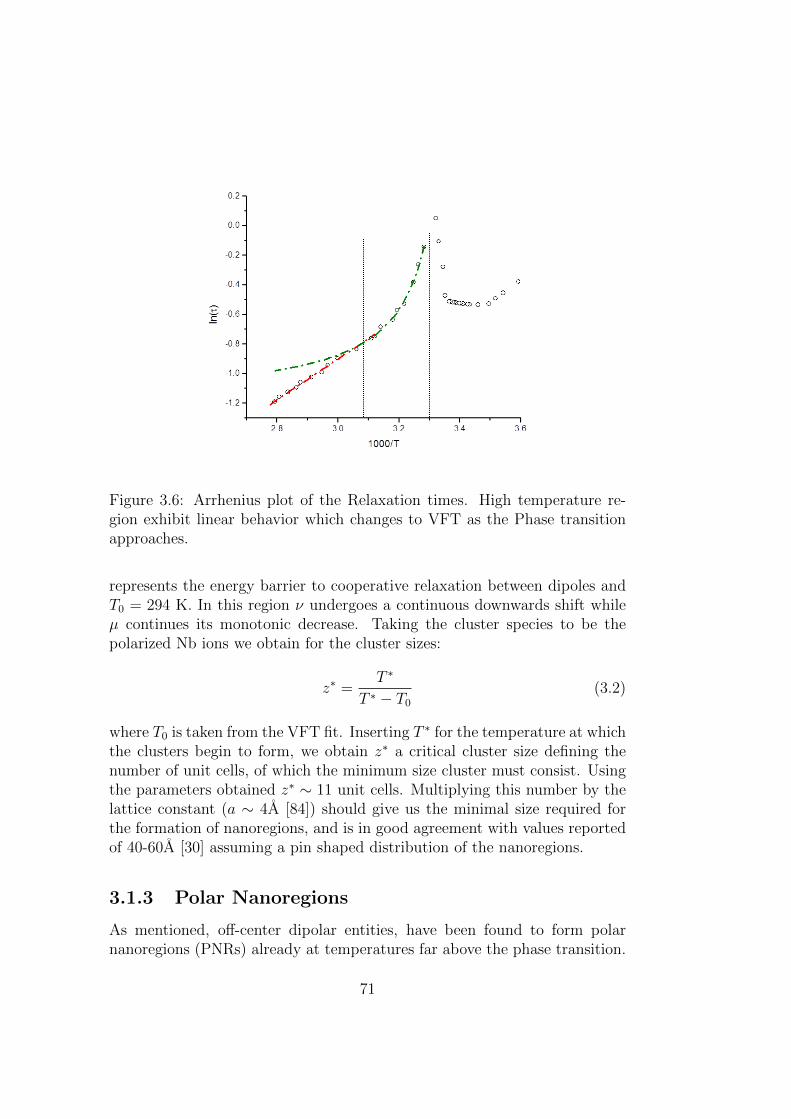
Figure 3.6: Arrhenius plot of the Relaxation times. High temperature re-gion exhibit linear behavior which changes to VFT as the Phase transitionapproaches.
represents the energy barrier to cooperative relaxation between dipoles andT0 = 294 K. In this region ν undergoes a continuous downwards shift whileµ continues its monotonic decrease. Taking the cluster species to be thepolarized Nb ions we obtain for the cluster sizes:
z∗ =T ∗
T ∗ − T0(3.2)
where T0 is taken from the VFT fit. Inserting T ∗ for the temperature at whichthe clusters begin to form, we obtain z∗ a critical cluster size defining thenumber of unit cells, of which the minimum size cluster must consist. Usingthe parameters obtained z∗ ∼ 11 unit cells. Multiplying this number by thelattice constant (a ∼ 4A [84]) should give us the minimal size required forthe formation of nanoregions, and is in good agreement with values reportedof 40-60A [30] assuming a pin shaped distribution of the nanoregions.
3.1.3 Polar Nanoregions
As mentioned, off-center dipolar entities, have been found to form polarnanoregions (PNRs) already at temperatures far above the phase transition.
71

The nanoregions are comprised of off-center ions whose relaxational behav-iors are correlated over mesoscopic length scales. The formation of thesenanoregions and their subsequent evolution has recently started to emergeas one of the key proponents governing phase transition dynamics.
The temperature where the polar nanoregions first become detectablewithin the lattice is known as the Burns or dipolar temperature, Td. Theirexistence was first detected by means of changes in the birefringence [29].Another signature is the appearance of elastic diffuse scattering [27]. Finallythis temperature can also be detected via accousto-optical methods [85].Recently an additional Intermediate Temperature T ∗ has been introduced.This is where the nanoregions start to interact with one another. At thistemperature, short-range correlations between these dipolar regions lead toa deviation from Curie-Weiss behavior in dielectric measurements.
Some confusion exists within the scientific literature, and these two tem-peratures are at different times both referred to as the Burns Temperature.This is due to historic developments, as the Burns temperature was discov-ered first and only recently as it become clear that this additional interme-diate temperature does indeed exist on its own. For purposes of clarity weshall try to clearly differentiate the two. In our case we are mainly interestedin T ∗ situated approximately 20 degrees above the Phase Transition. Theactual Burns Temperature in these crystals is actually much higher [85].
Evidence of this Intermediate temperature is evident from a number ofthe dielectric measurements presented. It is clearly seen in the deviationfrom Curie-Weiss in the dielectric strength, the deviation from Arrheniusbehavior in the relaxation time and the changes that begin to appear in thepower and stretch parameters (Figure 3.5). All of these instances are a clearindication that the dielectric measurements are indeed reflecting a processthat is revolving around clusterization.
The Burns temperature and the Intermediate temperature have been bothaccurately determined in these crystals [85]. The intermediate temperatureis evident in DSC measurements as well [76, 7]. The DSC result is presentedin figure 3.7. The picture alone immediately provides a qualitative indicationof the Burns Temperature at 323K, appearing as an exothermic peak in theheat capacity data. Such a peak is indicative of a crystal melt or phase tran-sition and can be quantified in terms of latent heat. This accurate value forthe Burns Temperature is in good agreement with the deviations mentionedabove in the dielectric measurements.
Anomalies in specific heat data around Td have been noted for a numberof relaxor ferroelectrics and have been attributed to the formation of thePNRs. The shape is qualitatively similar to that seen in PMN only theexcess is here much smaller. The excess here is compared to PMN in figure
72
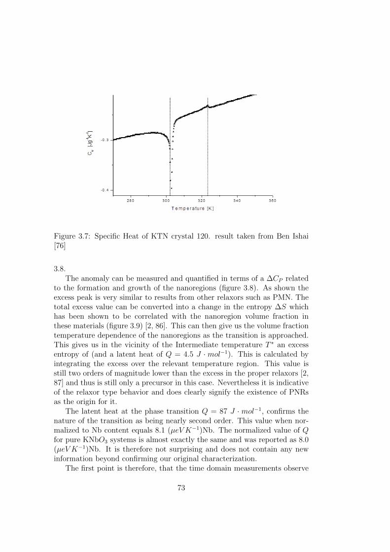
Figure 3.7: Specific Heat of KTN crystal 120. result taken from Ben Ishai[76]
3.8.The anomaly can be measured and quantified in terms of a ∆CP related
to the formation and growth of the nanoregions (figure 3.8). As shown theexcess peak is very similar to results from other relaxors such as PMN. Thetotal excess value can be converted into a change in the entropy ∆S whichhas been shown to be correlated with the nanoregion volume fraction inthese materials (figure 3.9) [2, 86]. This can then give us the volume fractiontemperature dependence of the nanoregions as the transition is approached.This gives us in the vicinity of the Intermediate temperature T ∗ an excessentropy of (and a latent heat of Q = 4.5 J · mol−1). This is calculated byintegrating the excess over the relevant temperature region. This value isstill two orders of magnitude lower than the excess in the proper relaxors [2,87] and thus is still only a precursor in this case. Nevertheless it is indicativeof the relaxor type behavior and does clearly signify the existence of PNRsas the origin for it.
The latent heat at the phase transition Q = 87 J ·mol−1, confirms thenature of the transition as being nearly second order. This value when nor-malized to Nb content equals 8.1 (µeV K−1)Nb. The normalized value of Qfor pure KNbO3 systems is almost exactly the same and was reported as 8.0(µeV K−1)Nb. It is therefore not surprising and does not contain any newinformation beyond confirming our original characterization.
The first point is therefore, that the time domain measurements observe
73

Figure 3.8: Temperature dependence of the anomalous Heat capacity inKTN. Very similar in form to the temperature dependence of the anoma-lous Heat capacity in PMN found in [86]
Figure 3.9: Relation between PNR volume ration and temperature as in-ferred from the specific heat measurements. Taken from [86] and [88] withpermission.
74
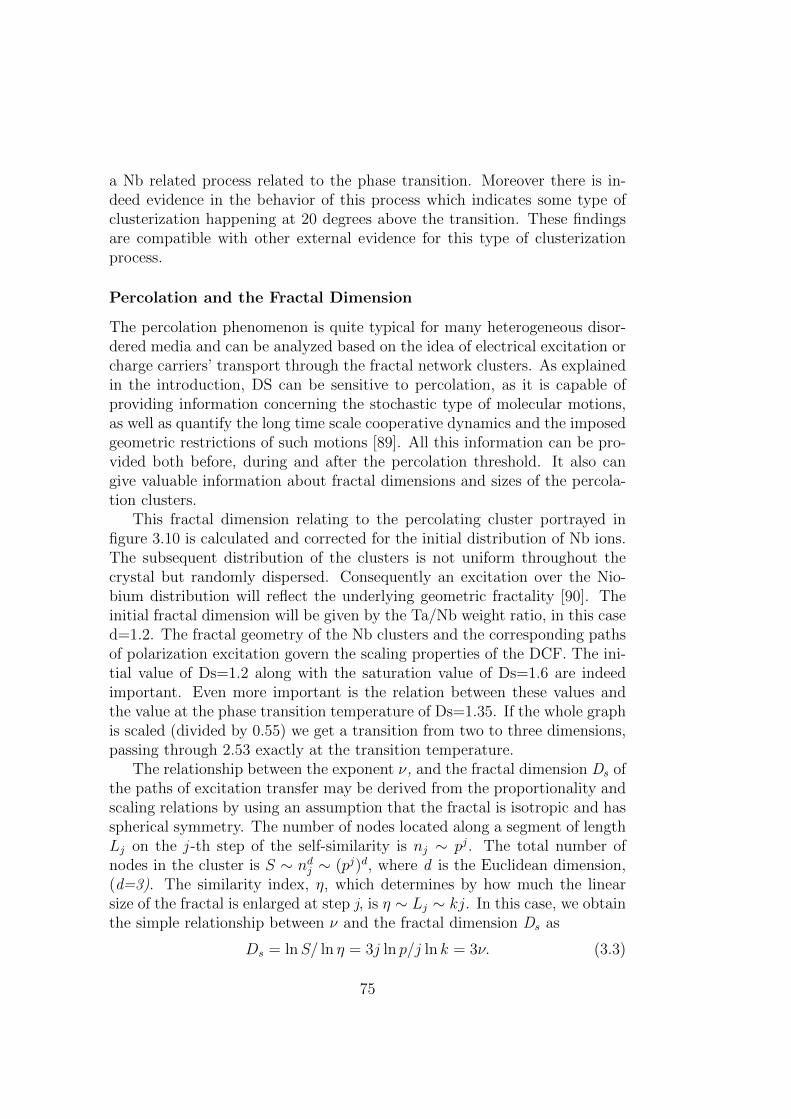
a Nb related process related to the phase transition. Moreover there is in-deed evidence in the behavior of this process which indicates some type ofclusterization happening at 20 degrees above the transition. These findingsare compatible with other external evidence for this type of clusterizationprocess.
Percolation and the Fractal Dimension
The percolation phenomenon is quite typical for many heterogeneous disor-dered media and can be analyzed based on the idea of electrical excitation orcharge carriers’ transport through the fractal network clusters. As explainedin the introduction, DS can be sensitive to percolation, as it is capable ofproviding information concerning the stochastic type of molecular motions,as well as quantify the long time scale cooperative dynamics and the imposedgeometric restrictions of such motions [89]. All this information can be pro-vided both before, during and after the percolation threshold. It also cangive valuable information about fractal dimensions and sizes of the percola-tion clusters.
This fractal dimension relating to the percolating cluster portrayed infigure 3.10 is calculated and corrected for the initial distribution of Nb ions.The subsequent distribution of the clusters is not uniform throughout thecrystal but randomly dispersed. Consequently an excitation over the Nio-bium distribution will reflect the underlying geometric fractality [90]. Theinitial fractal dimension will be given by the Ta/Nb weight ratio, in this cased=1.2. The fractal geometry of the Nb clusters and the corresponding pathsof polarization excitation govern the scaling properties of the DCF. The ini-tial value of Ds=1.2 along with the saturation value of Ds=1.6 are indeedimportant. Even more important is the relation between these values andthe value at the phase transition temperature of Ds=1.35. If the whole graphis scaled (divided by 0.55) we get a transition from two to three dimensions,passing through 2.53 exactly at the transition temperature.
The relationship between the exponent ν, and the fractal dimension Ds ofthe paths of excitation transfer may be derived from the proportionality andscaling relations by using an assumption that the fractal is isotropic and hasspherical symmetry. The number of nodes located along a segment of lengthLj on the j -th step of the self-similarity is nj ∼ pj. The total number ofnodes in the cluster is S ∼ nd
j ∼ (pj)d, where d is the Euclidean dimension,(d=3). The similarity index, η, which determines by how much the linearsize of the fractal is enlarged at step j, is η ∼ Lj ∼ kj. In this case, we obtainthe simple relationship between ν and the fractal dimension Ds as
Ds = lnS/ ln η = 3j ln p/j ln k = 3ν. (3.3)
75

Figure 3.10: Fractal dimension of the underlying lattice calculated based onthe ν parameter.
Focusing our attention primarily on the time dependent behavior of theDCF Ψ(t), in the simplified form
ψ(t) = C(t) exp[−(t/τ)Dp/3]. (3.4)
where C(t) is the slow growing function of time which accounts for a numberof the parameters in the power and stretch term together. By taking intoaccount (3.3) and ignoring the slow variation with time of C(t), and usingonly the asymptotic limit we obtain an even more simplified form leavingonly a stretched-exponential term with two parameters
ψ(t) ∼ exp[−(t/τ)Dp/3]. (3.5)
that can be fitted to the experimental correlation functions in order to de-termine the value of the fractal dimension of the paths of excitation transferwithin the system.
Feldman et al. [70], showed that for systems demonstrating self similarityon certain length scales (expected for polar nanoregions of Niobium clusteri-zation), the exponent ν could be further modified to reflect the spatial fractaldimension of the clusters
ν =Dg
3. (3.6)
76
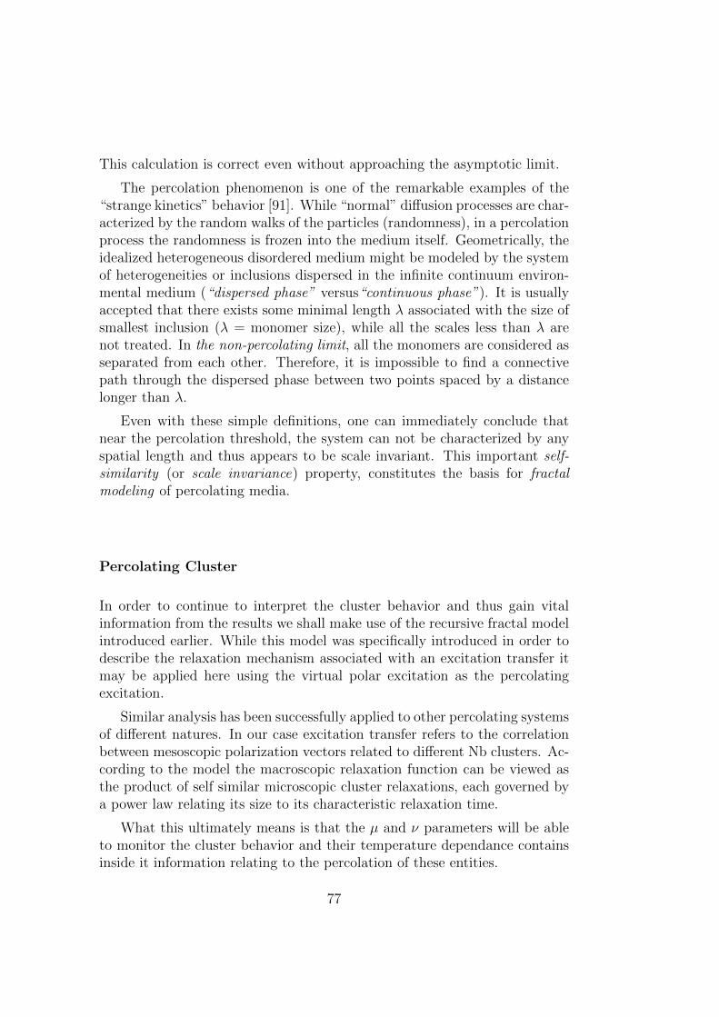
This calculation is correct even without approaching the asymptotic limit.
The percolation phenomenon is one of the remarkable examples of the“strange kinetics” behavior [91]. While “normal” diffusion processes are char-acterized by the random walks of the particles (randomness), in a percolationprocess the randomness is frozen into the medium itself. Geometrically, theidealized heterogeneous disordered medium might be modeled by the systemof heterogeneities or inclusions dispersed in the infinite continuum environ-mental medium (“dispersed phase” versus“continuous phase”). It is usuallyaccepted that there exists some minimal length λ associated with the size ofsmallest inclusion (λ = monomer size), while all the scales less than λ arenot treated. In the non-percolating limit, all the monomers are considered asseparated from each other. Therefore, it is impossible to find a connectivepath through the dispersed phase between two points spaced by a distancelonger than λ.
Even with these simple definitions, one can immediately conclude thatnear the percolation threshold, the system can not be characterized by anyspatial length and thus appears to be scale invariant. This important self-similarity (or scale invariance) property, constitutes the basis for fractalmodeling of percolating media.
Percolating Cluster
In order to continue to interpret the cluster behavior and thus gain vitalinformation from the results we shall make use of the recursive fractal modelintroduced earlier. While this model was specifically introduced in order todescribe the relaxation mechanism associated with an excitation transfer itmay be applied here using the virtual polar excitation as the percolatingexcitation.
Similar analysis has been successfully applied to other percolating systemsof different natures. In our case excitation transfer refers to the correlationbetween mesoscopic polarization vectors related to different Nb clusters. Ac-cording to the model the macroscopic relaxation function can be viewed asthe product of self similar microscopic cluster relaxations, each governed bya power law relating its size to its characteristic relaxation time.
What this ultimately means is that the µ and ν parameters will be ableto monitor the cluster behavior and their temperature dependance containsinside it information relating to the percolation of these entities.
77

uuu
uu u
2
2
2
2
2
2
Figure 3.11: Distribution of the nanoregions by size for different tempera-tures. Calculated based on the cluster distribution function using the re-sponse function fit parameters.
3.1.4 Cluster Distribution
The next vital piece of new information which we can learn from the measure-ments is the cluster distribution. This can be calculated from the percolationmodel introduced and is in fact directly related to it. The percolation modelassumed a specific type of cluster distribution function in order to obtainat last the DCF in the form of the power and stretch exponential (Equa-tion (1.54)). Using the µ and ν parameters from the fitting and doing thebackwards engineering we can reproduce the cluster distribution functionwhich would produce these values and uncover how it changes along withthe temperature.
The initial assumption of a cluster distribution function in the shape of
w(s) ∝ s−Ω exp(s
sm) (3.7)
is now plotted in Figure 3.11. This method is thus an effective way of mon-
78
Figure 3.12: Distribution of nanoregions in PMN-PT. Similar exponentialdependance as appears in the percolative model. Taken from [92] with per-mission.
itoring the distribution and sizes of the nanoregions as the phase transitionis approached. The basic form of the distribution has been independentlyconfirmed in both PMN-PT [92] as well as SBN [93] (Figure 3.12), usingpiezoelectric force microscopy [94]. While this method does indeed give a di-rect picture of the momentary distribution showing exactly where each andevery region lies along with its shape and size it is very time and resourceconsuming just to obtain one detailed snapshot at one particular tempera-ture. The method provided here only provides the statistical parameters butis a much more efficient way of actually probing and monitoring the materialover a wide temperature regime in order to study the dynamics.
To conclude this section of the discussion, we have shown so far the moni-toring of the PNRs and their dynamics as the phase transition is approached.These dynamics strongly influence the phase transition itself and may evenbe the main driving force behind it. The next section deals with the con-ductive hopping process in the lower frequency range. The study will probewhether or not it is affected by the changes in the underlying lattice and howthese changes can be enhanced through external parameters such as pressure.
79

3.2 Frequency Domain Results (I) -
Identifying the Electron Hopping Pro-
cess
3.2.1 Frequency Domain Results
Dielectric Landscape
In this section we present the results relating to a process which shall belater identified as an electron hopping process. We are mainly interestedhere in the behavior in the temperature regime above the phase transition(i.e. the Paraelectric phase) not due to any intrinsic reasons but rather dueto practical experimental limitations. As we shall see, the process is muchmore difficult to measure in the Ferroelectric phase as it lies on the borderof our low frequency measuring capabilities.
Previous work presented in the thesis of Dr. Paul Ben Ishai [88] demon-strated the typical ambient pressure measurements of a KTN crystal (num-bered crystal 120) and its dielectric analysis. Some of the analysis was takenand extended here further within the context of some of the new modelsdeveloped within the course of this study. These measurements served asbackground for the work following and also establish a reference with whichto compare the additional new measurements (i.e. low frequency and pres-sure measurements) performed within the framework of this study on thesame crystal.
Results for the dielectric landscape (of Crystal 120) are shown in figure3.13. The low frequency process (Process A) seen in the figure is universallyfound in all crystals with varying levels of Nb, and independent of Cu andLi concentrations. also noted is Process B - the higher frequency processrelated to Cu, which shall not be dealt with in depth in this study.
Of the crystal used exclusively for this study, first presented are the resultsfor Crystal 100 which was measured in order to combine these results withthe TDS measurements presented in the previous section. This allows us topresent a comprehensive picture consisting of a very wide range of frequencyscales covered by the measurements. The results of the BDS measurementsof this crystal are indeed qualitatively quite similar to the measurements ofCrystal 120 except for the fact that there was no trace of a higher frequencyCu related process (labeled in previous research as Process B). Both themeasurements of Crystal 120 as well as those of Crystal 100, also serve as areference point for the low frequency measurements performed on crystal .
In the measurements made in these type crystals it has been shown that
80

Figure 3.13: Dielectric landscape in the typical case (here crystal 120). Thecrystal exhibits a number of relaxation processes in different frequency re-gions. Taken from the thesis of Dr. Paul Ben Ishai, with permission [88].
81

Table 3.1: Comparison between Activation Energy obtained from Process A,∆Eτ , and the Activation Energy related to the DC conductivity, ∆Eσ for anumber of different crystals with various dopant compositions.Crystal Nb conc. Cu conc. Li conc. ∆Eτ [eV] ∆Eσ[eV]077 Nb 21% no Cu no Li 0.69±0.01 0.65±0.04100 Nb 35% no Cu no Li 0.86±0.01 0.99±0.01110 Nb 38% no Cu 2.4% Li 0.86±0.01 0.85±0.01120 Nb 38% 2% Cu no Li 0.94±0.01 0.95±0.01083 Nb 38% 2% Cu 2.8% Li 0.90±0.01 0.99±0.019038 Nb 38% 2% Cu 2.4% Li 0.94±0.01 0.95±0.01
the relaxation process bears a strong connection to the DC conductivity [76]as shown in Table 3.1. This will be taken from the Activation energy values,taken from the plots of the relaxation times, compared with the Conduc-tivity activation energies. These measurements come from both the crystalsmeasured directly in this study (100, 120, 9038) as well as the previouslymeasured crystals.
The correlation between these different Activation Energies is the firsthint of a possible link to electron hopping as it strongly suggests that boththe conductivity and the dielectric process share a common origin. The focuswithin the limited context of this research will be on this process, and as inprevious studies [76] it shall usually be referred to as Process A.
3.2.2 Low Frequencies
As mentioned one crystal was measured at very low frequencies. In thiscase, as in all of the previous instances, the electron hopping related ProcessA showed the typical Arrhenius relaxation (Figure 3.14)(a), with activationenergy equal to that of the DC conductivity (Figure 3.14)(b). Also presentwas the Cole-Cole broadening (Figure 3.14)(c) along with the Curie-Weissdependence in the dielectric strength (Figure 3.14)(d). Once again the shapeof the graph in the Paraelectric phase is qualitatively similar to both crystals100 and 120.
The new information provided in this case is from the area in the vicinityof the phase transition. In this regime the relaxation has move to the lowend of the measurement capabilities residing in the 10−2− 10−4Hz frequencyrange. It is in this area where the underlying lattice is in the midst ofundergoing major transformations where it should prove most interesting toanalyze the obtained relaxation parameters. They should be able to provideadditional insight as to what is taking place at the mesoscopic level as the
82
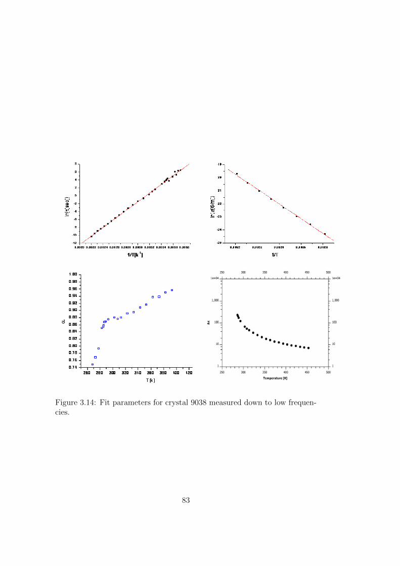
Figure 3.14: Fit parameters for crystal 9038 measured down to low frequen-cies.
83

2.2 2.4 2.6 2.8 3.0 3.2 3.4 3.6-5
-4
-3
-2
-1
0
1
2
ln(
[sec
])
1000/T
Figure 3.15: Dielectric relaxation time Fit Parameter τ for a number of dif-ferent crystals with different crystal constituents. Symbols represent differentcrystals : (×) 100, () 120, () 077, (+) 083, () 9038.
transformation is underway.
3.2.3 Changing Concentration
Two more points need to be mentioned regarding the relaxation process andas initially in the thesis of Dr Ben Ishai [88]. These relate to the measure-ments of the additional crystals beyond crystals 100, 120, and 9038. The firstrelates to the relaxation times for Process A. In all of the additional crystalsmeasured with various Cu and Li concentrations (and one with a very differ-ent Nb concentration), the process continued to exhibit the same Arrheniusbehavior. As mentioned before all crystals showed a correlation between therelaxation activation energy and that of the conductivity. The value of thisActivation energy was found to be weakly concentration dependant. This isshown in figures 3.15 and 3.16. The variance in the activation energy will beused later on, in order to extract vital information regarding the system.
The second point relates to the loss broadening. As shown the loss broad-ening of the three crystals focused on in this study shared very similar fea-tures in the paraelectric regime. This does not hold true for many of theother crystals measured. There the behavior of the loss parameter can bequite varied. The reasons were explained in depth in the work of Dr. BenIshai and will be touched upon in the discussion section.
84

Figure 3.16: Dielectric relaxation Fit Parameter α for a number of differ-ent crystals with different crystal constituents. Symbols represent differentcrystals : (×) 100, () 120, () 077, (+) 083, () 9038.
3.2.4 Frequency Domain Interpretation
Fitting of the dielectric process observed in all of the Ferroelectric crystalsused in this study proceeded as described above according to equation(1.20)using a single symmetric loss peak (Cole-Cole). The features and their cor-responding parameters in the CC equation are:
1. The amplitude of the process ∆ǫ, related to the number of relaxingentities and the main focus of this thesis,
2. The symmetric broadening of the loss peak, expressed through the CC,α parameter.
Two more features are related to the relaxation time, τ , namely:
1. The activation energy ∆E, reflecting the energetic landscape,
2. The relaxation prefactor τ0.
As will be demonstrated, the behavior of these parameters may be wellexplained under the electron hopping assumption [76, 95].
The full frequency spectrum containing both the dielectric permittivityand losses as functions of frequency and temperature were measured as de-scribed in the preceding chapter. The results of the fitting parameters at eachtemperature point will be presented here for each individual crystal. Also
85

shown is the fitting parameter for the DC conductivity showing its correlationwith the relaxation times.
We now proceed to look at the fitting results of the frequency domainmeasurements, specifically investigating the process labeled as Process A.All of the symptoms do indeed imply that electron hopping is indeed at theheart of Process A. In relation to this, all four of the relaxation parametersenumerated previously are of distinct importance. Some of these parametersare simply consistent with the electron hopping model, while others actuallyprovide strong evidence promoting this interpretation.
1. The activation energy ∆E, reflecting the energetic landscape. The Ar-rhenius behavior of all compositions and at all pressures is not indeedunique to electron hopping. However, the strong correlation betweenthese activation energies and the corresponding activation energies ofthe DC conductivity strongly suggest a common origin.
2. The minimum relaxation time τ0. In conjunction with the Meyer-Neldelcompensation law which shall be introduced this parameter can indicatewhether we are dealing with a process governed by a single excitation orone which necessitates a simultaneous congregation of multi excitations.The latter does indeed indicate a process relying on entities, such aselectrons, sitting in deep traps and other entities, such as phonons,that can come together statistically in large numbers and serve as adriving force. This is indeed the case for polaron like electron hoppingprocesses [96].
3. The symmetric broadening of the loss peak, expressed through the CC,α parameter. In line with the aforementioned ideas of Ryabov [97], ifthe time set of interactions demonstrates self similarity at some scale,then it would be expected that the process would indeed exhibit Cole-Cole behavior.
This symmetric broadening would be consistent with a hopping process.Such a process is expected to be strongly influenced by the self-similarlandscape while relatively immune to the non-symmetric direct dipole-dipole interactions (which usually result in Cole-Davidson behavior).
In fact Process A does indeed demonstrate Cole-Cole behavior at allmeasured pressures. Thus the α parameter should contain significantinformation on the dynamics of the hopping.
4. The amplitude or dielectric strength of the process ∆ǫ. This parameteris related to the number of relaxing entities. Within the framework of
86

the electron hopping model we shall develop a model to calculate thedegree of correlation between such hopping entities.
We shall now describe each of the above points at greater length, detailinghow each part fits into the larger picture of the hopping process and whatcan be derived from applying this model.
Relaxation Times
First presented are the results for τ the relaxation times of this identifiedprocess. These results do not merit a new devoted section as they are mostlystraightforward and do not provide many new insights. Figure 3.17(a) showsthe typical case for a crystal at nominal ambient pressure. It show the dataobtained from crystal 120, which as shall be seen is quite typical in thisregard.
The relaxation time has as noted the normal Arrhenius dependence. Theactivation energy is noted in Table 3.1. Figure 3.17(b) shows the DC con-ductivity with its corresponding Activation energy also noted in Table 3.1.As mentioned these two are very close in value.
Next presented are the results for τ the relaxation times for the dataobtained from crystal 100 (Figure 3.18(a)). The data is qualitatively similarto crystal 120. The relaxation time has once again the normal Arrheniusdependence. The activation energy is noted in Table 3.1. Figure 3.18(b)shows the DC conductivity with its corresponding Activation energy alsonoted in Table 3.1. Here too the values are once again very close to eachother.
3.3 Frequency Domain Results (II) -
Dipole-Lattice Interaction
Cole Cole Broadening
The second quadrant of the graph (Figure 3.17, Figure 3.18) presents theresults for α the loss broadening of this identified process. Figure 3.17 forcrystal 120 and Figure 3.18 for crystal 100. Here too the qualitative behavioris very similar and the shapes of these two graphs bear many features incommon.
In previous studies it was conclusively shown that the behavior of α isrelated to the interactions with the underlying lattice. This is due to the factthat relaxation events are in the general case, never completely isolated andtherefore never totally independent of one another. They can to a certain
87
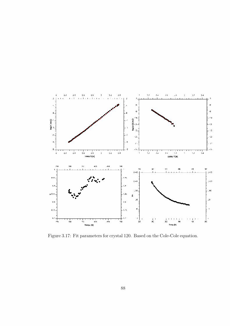
Figure 3.17: Fit parameters for crystal 120. Based on the Cole-Cole equation.
88
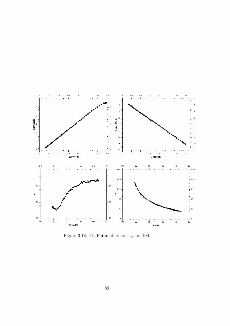
Figure 3.18: Fit Parameters for crystal 100.
89

extent be influenced through dipolar interactions. This happens both withneighboring dipoles as well as with the underlying matrix itself.
3.3.1 Alpha Tau Relation
This relationship between the dipoles and the underlying lattice is expressedthrough the symmetric loss broadening. The broadening is indicative of adipole-matrix interaction mediating the process, and is thus completely con-sistent with the electron hopping model. The fractional derivative formalismapplied in order to analyze this was put forward by by Ryabov [97].
This analysis leads to the conclusion that symmetric CC broadening ofthe loss peak is a result of the interaction between the microscopic elements ofthe ensemble with their surroundings. The parameter α in the CC equationis the fractal dimension of the time set defined by
α =ln(N)
ln(ξ)(3.8)
where N is the number of interactions in the time set defined by the dimen-sionless time parameter ξ. For transport processes involving self diffusionthey derived a simplified relationship between the structural parameters ofthe system and the parameters of the CC equation
α =DG
2
(ln (ωsτ)
ln (τ)− ln (τ0)
)(3.9)
where DG is related to the spatial fractal dimension, τ the relaxation time forthe process, ωc is the characteristic frequency for the self diffusive transportand τ0 is a microscopic cut off time for the diffusive process.
If the time set of interactions demonstrates self similarity at some scale,then it would be expected that the process would exhibit Cole-Cole behavior,in line with these ideas of Ryabov and Feldman [97]. If this is indeed the casethan the α parameter would contain significant information on the dynamicsof the hopping. In fact in all of the KTN crystals presented here, ProcessA does indeed demonstrate Cole-Cole behavior. Figure 3.19 goes one stepfurther and shows the α − τ relationship for the two crystals (100 and 120)measured. They can both be well fit to the model at least in the paraelectricphase down to T ∗.
An additional feature that emerges from the above formalism is the ap-pearance of the intermediate T ∗ temperature [30] (the temperature in be-tween the Burns TD [29], and the Critical phase transition temperature TC).There is a clearly evident shift of behavior change in the results appearing
90
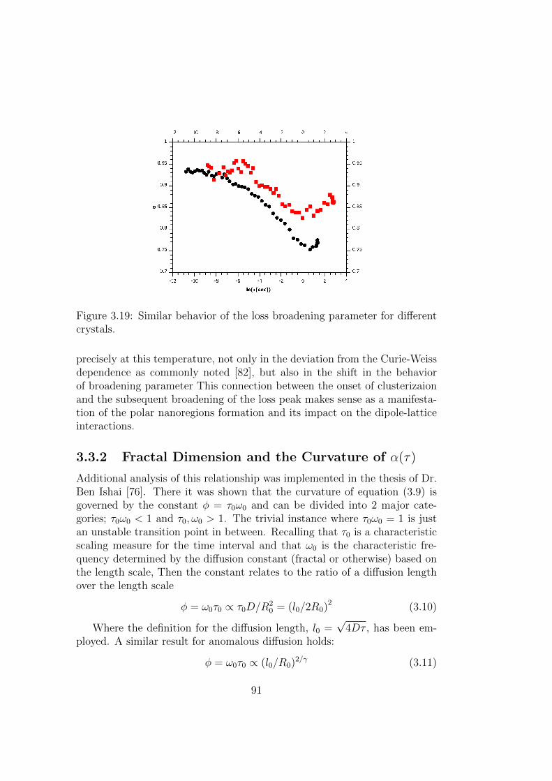
Figure 3.19: Similar behavior of the loss broadening parameter for differentcrystals.
precisely at this temperature, not only in the deviation from the Curie-Weissdependence as commonly noted [82], but also in the shift in the behaviorof broadening parameter This connection between the onset of clusterizaionand the subsequent broadening of the loss peak makes sense as a manifesta-tion of the polar nanoregions formation and its impact on the dipole-latticeinteractions.
3.3.2 Fractal Dimension and the Curvature of α(τ)
Additional analysis of this relationship was implemented in the thesis of Dr.Ben Ishai [76]. There it was shown that the curvature of equation (3.9) isgoverned by the constant φ = τ0ω0 and can be divided into 2 major cate-gories; τ0ω0 < 1 and τ0, ω0 > 1. The trivial instance where τ0ω0 = 1 is justan unstable transition point in between. Recalling that τ0 is a characteristicscaling measure for the time interval and that ω0 is the characteristic fre-quency determined by the diffusion constant (fractal or otherwise) based onthe length scale, Then the constant relates to the ratio of a diffusion lengthover the length scale
φ = ω0τ0 ∝ τ0D/R20 = (l0/2R0)
2 (3.10)
Where the definition for the diffusion length, l0 =√4Dτ , has been em-
ployed. A similar result for anomalous diffusion holds:
φ = ω0τ0 ∝ (l0/R0)2/γ (3.11)
91
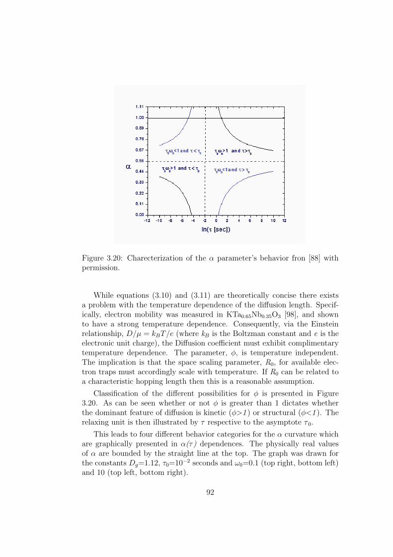
Figure 3.20: Charecterization of the α parameter’s behavior fron [88] withpermission.
While equations (3.10) and (3.11) are theoretically concise there existsa problem with the temperature dependence of the diffusion length. Specif-ically, electron mobility was measured in KTa0.65Nb0.35O3 [98], and shownto have a strong temperature dependence. Consequently, via the Einsteinrelationship, D/µ = kBT/e (where kB is the Boltzman constant and e is theelectronic unit charge), the Diffusion coefficient must exhibit complimentarytemperature dependence. The parameter, φ, is temperature independent.The implication is that the space scaling parameter, R0, for available elec-tron traps must accordingly scale with temperature. If R0 can be related toa characteristic hopping length then this is a reasonable assumption.
Classification of the different possibilities for φ is presented in Figure3.20. As can be seen whether or not φ is greater than 1 dictates whetherthe dominant feature of diffusion is kinetic (φ>1 ) or structural (φ<1 ). Therelaxing unit is then illustrated by τ respective to the asymptote τ 0.
This leads to four different behavior categories for the α curvature whichare graphically presented in α(τ) dependences. The physically real valuesof α are bounded by the straight line at the top. The graph was drawn forthe constants Dg=1.12, τ0=10−2 seconds and ω0=0.1 (top right, bottom left)and 10 (top left, bottom right).
92

3.4 Frequency Domain Results (III) -
Dipole-Dipole Interaction
3.4.1 Dielectric Strength and Dipole Correlation
Dielectric Strength
After the relaxation time and broadening, the next parameter extracted fromthe dynamic analysis is the dielectric strength of the process.
Presented in Figures 3.17(d) and 3.18(d) are the results for this ∆ε re-laxation strength of the identified process.
Typically this should be related to the number of dipolar entities takingpart in the relaxation event, as shown in the original works of Frohlich [73].However, in order to properly factor in the contribution of each of the dipolarentities the degree of correlation must also be taken into account. Alterna-tively, it may be this very correlation factor and its behavior, which we wantto investigate.
Dipole Correlation
The typical approach taken in order to relate ∆ε to the number and cor-relation of dipolar interactions, is demonstrated through the Frohlich B(T )function:
B (T ) =4π
3
N0
k〈mm∗〉 =
(ǫs − n2
) 2ǫs + n2
3ǫsǫ0T (3.12)
For typical materials the slope of the B function usually indicates whether ornot there is a tendency for parallel of anti-parallel dipolar alignment withina certain region. Construction of the Frohlich B(T ) function, can provideadditional information regarding the number of relaxing entities and thenature of the interactions between them. The behavior of these crystals isstrangely similar to that found in dipolar liquids [73]. This appearance ofliquid like behavior inside the lattice of a well organized solid is at first glancepuzzling. It is vaguely reminiscent of some other strange liquid like behaviorin some of these crystals [36]. It would seem to indicate that the observedprocess contains some feature whose relaxation is not directly bound to thelattice itself but rather a distinct entity operating within the lattice confines.This fits in well with the assumption that the process we are investigating isrelated to free electrons and not to the ions constituting the lattice itself.
The appearance of the liquid like behavior in the behavior of the FrohlichB(T ) function was taken as an indication as to the independent nature ofthe observed process from the crystal lattice. The problem however with
93
the direct application of the Frohlich B(T ) function is that is technicallynot suited for the type of case at hand. The derivation assumes a fixeddipolar length for the various dipoles which are then averaged in a certainregion. This is not the case when the dipole under consideration is a changingvirtual dipole, which is constantly varying in size and direction due to theperturbations of the lattice. In order to obtain meaningful values and aproper estimation of the number of interacting entities the methodology mustbe adapted. Using methods based on the original approach of Kirkword [74]and Frohlich [73] a new definition can be introduced for the dipole-dipolecorrelation factor based on the dielectric strength, ∆ǫ, by comparing thefree energy associated with a polaron hop to the free energy associated witha dipole moment [91]. This first allows us to calculate the free electrondensity from which we can afterwards extract the pressure dependence andthe effective correlation.
The main limitation of this model is that it is strictly applicable onlyfor systems which can be represented as a sphere, neatly divided up into Nmicroscopic cells, Fig.3.21(a). No such theory is available as yet for the case ofvirtual dipoles as they offer no direct approach to estimate the contribution ofa single entity to the overall dielectric strength. Even if we are able to assumea specific distribution of dipole moments with varying lengths, Fig.3.21(b),the decoupling still remains a complex problem.
In order to circumvent the limitations inherent in the above model, wetake into account the temporal evolution of the virtual dipole and introducean alternate representation based on the average mean square displacementvalues, Fig.3.21(c). This enables extending the model to include any type ofapparent dipole moment occurring in a system linked to electron hopping orother types of transport.
The size of spherical region under consideration must now be large inrelation to the mean path length transversed within the duration of therelaxation. Figure 3.21(d) concludes the schematic representation of theentire derivation.
3.4.2 Adapted Kirkwood Frohlich Model
We now introduce here the full derivation of the equation by which a neweffective correlation function is calculated. The starting point is still inspiredby Froehlich’s original ideas but adapted to a wider range of materials. Start-ing with the formula for the free energy of an electric moment in a cavity
94

Figure 3.21: (a) Standard case of fixed dipoles used in Frohlich’s originalderivation. (b) Non-fixed virtual dipoles. (c) Representation of virtualdipoles as products of a time averaged random walk. (d) Unpacking thevirtual dipoles by integrating out the time dimension, analogous to the orig-inal situation having only replaced the units of measure.
95
sphere surrounded by a dielectric
F =2π 〈M2〉
V
3εsε0 (2εs + ε∞) (εs − ε∞)
(3.13)
Where V is the volume of the sample, M is the electric moment and ǫs isthe static dielectric constant and ǫ∞ the high frequency limit.
The initial problem concerns correctly calculating the electric moment ofthe cavity, when the macroscopic dipole in question, 〈M2〉, is the result of anon rigid virtual dipole. In this case we start from the basic definition of theelectrical macroscopic dipole moment at time t.
⟨M2(t)
⟩=
⟨∑
i,j
q2 · ~ri (t) · ~rj (t)⟩
(3.14)
Equation 3.14 is an instantaneous snapshot of the ensemble average. Con-sidering we are viewing in our measurement window the time averaged valueof this ensemble. Furthermore, inside our time window we must appreciatethat the hop act depends upon the act before it and that it will influence theact occurring after it. Consequently one must not consider a simple averageon r2(t), but rather consider a memory function approach to the averaging
⟨M2⟩= lim
T→∞
1
T 2
∫∫ ⟨∑
i,j
q2 · ~ri (t) · ~rj (t− t′)
⟩dtdt′ (3.15)
If the system approaches the ergodic limit we are allowed to swap the timeand ensemble averages, obtaining:
⟨M2⟩=
⟨limT→∞
1
T 2
∫ ∫ ∑
i,j
q2 · ~ri (t) · ~rj (t− t′) dtdt′⟩
(3.16)
This is desirable because for a transport that is diffusive in nature we dohave an estimation of these quantities, namely mean square displacement,R2=Dτα , and as Cole-Cole can be derived using the anomalous diffusionequation we can assume that the transport properties of the electron hoppingare diffusive.
Ergodicity Breaking and Fractal Landscapes
Although it is most likely that we are dealing with an ergodic system sincecannot readily assume that the situation must be Ergodic, the next step is tooutline under what exact conditions we can justify swapping the time integral
96
and the summation of the space. If we can justify this even in the weaky non-ergodic case it will certainly be applicable in the cases of anomalous diffusionarising from the fractal nature of the landscape even when ergodicity breakingis not necessarily invoked.
There are a number of conditions that justify this act:
1. The hopping electron density is such that we can be considered as inthe dilute limit, meaning that each hopping entity is independent of theothers and does not interact with them. In this case each can be con-sidered as a sub-ensemble in the phase space describing the statisticalmechanics of the hopping system.
2. The ensemble average of equation becomes an averaging over the sub-ensembles. Consequently the time averaging act is now reduced to thetime average of the single entity.
In this case, for the single entity we can swap the time averaging with theensemble average. Mathematically stated we start by denoting the ensembleas the average of its statistically independent sub ensembles, denoted by thesubscript p. Each sub-ensemble corresponds to a particular subregion of thephase space accessible to be fully explored by the sample within a given timeframe [99, 100]. Being in the dilute limit the sub-ensembles can actuallybe taken to correspond to a single dipolar entity provided that the timewindow and sample size are large enough. This assumption is what allows usto simply treat each dipole independently and obtain the total average viasummation. The full ensemble average can then be expressed as
〈M2〉E = limp→∞
1
p
p∑
i=1
M2i (t) (3.17)
Using the relation which then equates the ensemble average of a timeaveraged quantity with the effective ensemble average [100]
〈〈M2p 〉T 〉E = lim
p→∞1
p
p∑
i=1
〈M2i 〉T = 〈M2
p 〉E (3.18)
allows us to compare the ensemble average obtained in this method with theensemble average obtained under ergodic assumptions.
⟨M2⟩=⟨⟨M2
p
⟩p
⟩T= lim
T→∞
1
T 2
∫∫dtdt′ lim
p→∞1
p
∑
p
M2p (3.19)
Because of the dilute limit there is no restriction in swapping the integral withthe summation (the sub ensembles do not interact and can be considered as
97

independent), taking the limits we achieve equation (3.19). Before carryingout the integral we can look further into the summation
⟨M2⟩= lim
T→∞
1
T 2
∫ ∫ ⟨∑
i,j
q2 · ~ri (t) · ~rj (t− t′)
⟩dtdt′ (3.20)
⟨M2⟩= lim
T→∞
q2
T 2
∫ ∫ (∑
i=j
〈ri (t) · ri (t− t′)〉+∑
i 6=j
〈~ri (t) · ~rj (t− t′)〉)dtdt′
(3.21)The summed values in equation 3.21 can now be recognized as an auto cor-relation and self correlation of the hopping electron as it moves through suc-cessive hops inside the time averaging window. Swapping the integrals withthe summations as defined above the first term is simply the mean squaredisplacement of the hop multiplied by the number of such acts, expressed asthe Volume, V, multiplied by the density, n0,
⟨M2⟩= V n0e
2⟨R2
rms
⟩+ V n0e
2 (z cos θ)⟨R2
rms
⟩(3.22)
If we approximate the second summation as a short term memory functionof how each hop will define it successor then we can approximate it by anaveraged angle, θ, from the start of the averaging window and a factor, z,indicating how many individual hops are relevant
Estimating the electric moment M from the root mean square length ofthe hop 〈R2
rms〉 = Dτα using the anomalous diffusion constant D, and therelaxation time; ⟨
M2⟩≈ V n0q
2Dτgeff (3.23)
Using the equivalent correlation factor: geff = 1 + z 〈cos (θ)〉Due to the fact that we are in the dilute limit, correlations will be limited
to the self correlations in the hopping direction of a single dipole. Underthis approximation this can be expressed through the off diagonal term ineq. 3.21 usually related to nearest neighbor correlations. Instead it nowaccounts for the number of hops related to one particular dipole z and theself correlation measure between two successive hops 〈cos (θi,j)〉 differing indirection by the angle θi,j . The right hand side relates to what will be calledan equivalent correlation factor geff = 1 + z 〈cos (θ)〉. Only now, instead ofrepresenting a sphere with a fixed dipole interacting with z neighbors at aneffective internal angle θ, it now represents a self correlation in the directionof successive electron hops. Within the measurement time window, a num-ber, z, of different hop interactions produce an effective hopping angle, θ.
98

This stipulation does places one restriction on the theory, not present in theoriginal Kirkwood Frolich model. The size of spherical region under consid-eration must now be large in relation to the mean path length transversedwithin the duration of the relaxation.
Polaron Free Energy
The final part of the derivation just requires substituting various parametersand formulas in order to actually calculate the free energy based on the aboveassumptions. Using the evaluation of the average dipole moment equation(3.13) now becomes
∆F =2πV n0q
2Dτ · geffV
3εsε0 (2εs + ε∞) (εs − ε∞)
(3.24)
Assuming an Arrhenius dependence of the relaxation time, we now substitute: τ = τ0 exp
(∆EkT
)obtaining
∆F = 2πn0e2Dτ0 exp (∆E/kT )
3εsε0 (2εs + ε∞) (εs − ε∞)
geff (3.25)
It is possible to express the diffusion coefficient in terms of the mobility, asthis quantity has been measured in our initial model system (Figure 3.22)[101].Where Epol is the polaron binding energy, the short range component of thefree energy, and T is the temperature. Based on this formulation we mayextract an expression for the number density of hopping electrons. This isimportant because this is an independently measured quantity and can befound in the literature.
n0 =(2πekµ0τ0)T
−1/2
∆F · geff
(3εs
ε0 (2εs + ε∞) (εs − ε∞)
)exp
(−Epol +∆E
kT
)
(3.26)The final piece of the puzzle is to decipher what is the free energy of the
cavity. We make the assumption, based on the conservation of energy thatthe Free energy of the cavity , as defined by equation is equated to the freeenergy permitting hopping.
Viewing the hop as a simple two level energy problem, where by theenergy required to elevate the electron from the trap in the band gap to theconduction band is given by ∆E. As the single electron in the dilute limitconsidered above , is a canonical ensemble the probability to find the electronin the elevated energy state (the conduction band) is given by the Boltzman
99
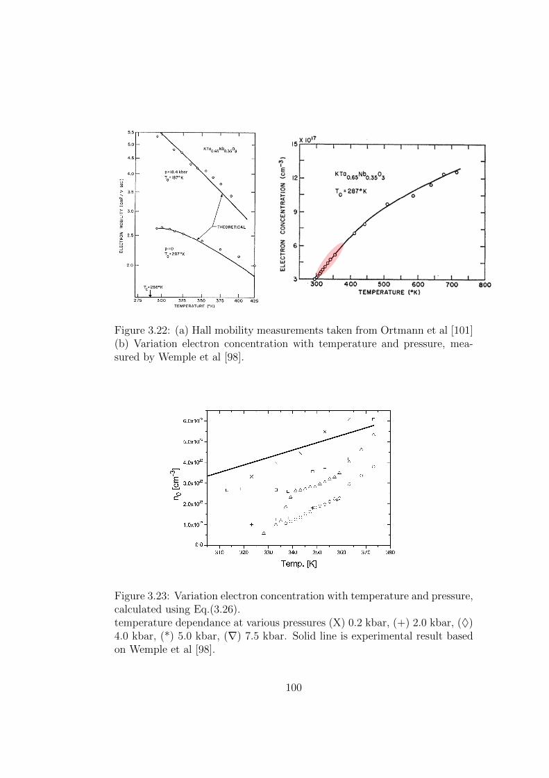
Figure 3.22: (a) Hall mobility measurements taken from Ortmann et al [101](b) Variation electron concentration with temperature and pressure, mea-sured by Wemple et al [98].
Figure 3.23: Variation electron concentration with temperature and pressure,calculated using Eq.(3.26).temperature dependance at various pressures (X) 0.2 kbar, (+) 2.0 kbar, (♦)4.0 kbar, (*) 5.0 kbar, (∇) 7.5 kbar. Solid line is experimental result basedon Wemple et al [98].
100

distribution function
P ∝ exp
(−∆F
kT
)(3.27)
Where k is Bolztman’s constant and ∆F is the free energy defined by
∆F = T∆S −∆E (3.28)
Noting that the characteristic relaxation time, τ , depends on the reciprocalof the probability, we can write the following
τ ∝ P−1 ∝ exp
(∆E − T∆S
kT
)= exp
(−∆S
k
)exp
(∆E
kT
)(3.29)
The last term of equation (3.29) can be recognized as the activation energy ofthe Arrhenius fit of the experimental relaxation times. Using the estimationbased on the observed MN dependance whereby ∆S/k=b∆E, we can writethe free energy as
∆F = T∆S −∆E = (Tkb− 1)∆E = (T/TMN − 1)∆E (3.30)
3.4.3 Effective Correlation Factor
The final equation for the effective correlation factor now takes the form of:
geff =1
KT 1/2
(ε0 (2εs + ε∞) (εs − ε∞)
3εs
)−1 exp(
−Epol+∆E
kT
)
(T/TMN − 1)∆E(3.31)
with K = (2πτ0kµ0e)−1
While the above equation does contain many different parameters, themajority of them can be taken directly from the scientific literature. Therest are determined from the dielectric relaxation function leaving a verydirect method of ascertaining the correlated behavior of the dipole ensemble.The more pronounced the loss peak for a particular transport process theless room there will be to modify the fit function providing a more preciseevaluation of the effective correlation.
Analysis of the correlation factor, g, now proceeds according to equation3.31 above. Depending on the system and what we can gather relating to itsvarious components, will determine how best to proceed with the calculationcorrelated behavior of the dipoles.
Much information can now be derived regarding the polaron propertiesof the transient process. Utilizing the measured Arrhenius dependence ofthe relaxation and inserting all of the parameters into equation 3.31, yields
101
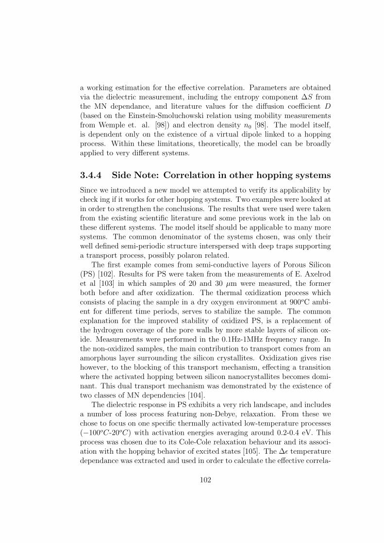
a working estimation for the effective correlation. Parameters are obtainedvia the dielectric measurement, including the entropy component ∆S fromthe MN dependance, and literature values for the diffusion coefficient D(based on the Einstein-Smoluchowski relation using mobility measurementsfrom Wemple et. al. [98]) and electron density n0 [98]. The model itself,is dependent only on the existence of a virtual dipole linked to a hoppingprocess. Within these limitations, theoretically, the model can be broadlyapplied to very different systems.
3.4.4 Side Note: Correlation in other hopping systems
Since we introduced a new model we attempted to verify its applicability bycheck ing if it works for other hopping systems. Two examples were looked atin order to strengthen the conclusions. The results that were used were takenfrom the existing scientific literature and some previous work in the lab onthese different systems. The model itself should be applicable to many moresystems. The common denominator of the systems chosen, was only theirwell defined semi-periodic structure interspersed with deep traps supportinga transport process, possibly polaron related.
The first example comes from semi-conductive layers of Porous Silicon(PS) [102]. Results for PS were taken from the measurements of E. Axelrodet al [103] in which samples of 20 and 30 µm were measured, the formerboth before and after oxidization. The thermal oxidization process whichconsists of placing the sample in a dry oxygen environment at 900oC ambi-ent for different time periods, serves to stabilize the sample. The commonexplanation for the improved stability of oxidized PS, is a replacement ofthe hydrogen coverage of the pore walls by more stable layers of silicon ox-ide. Measurements were performed in the 0.1Hz-1MHz frequency range. Inthe non-oxidized samples, the main contribution to transport comes from anamorphous layer surrounding the silicon crystallites. Oxidization gives risehowever, to the blocking of this transport mechanism, effecting a transitionwhere the activated hopping between silicon nanocrystallites becomes domi-nant. This dual transport mechanism was demonstrated by the existence oftwo classes of MN dependencies [104].
The dielectric response in PS exhibits a very rich landscape, and includesa number of loss process featuring non-Debye, relaxation. From these wechose to focus on one specific thermally activated low-temperature processes(−100oC-20oC) with activation energies averaging around 0.2-0.4 eV. Thisprocess was chosen due to its Cole-Cole relaxation behaviour and its associ-ation with the hopping behavior of excited states [105]. The ∆ǫ temperaturedependance was extracted and used in order to calculate the effective correla-
102

Figure 3.24: Effective correlation function gfactor = 1+ z 〈cos θ〉 for OxidizedPorous Silicon for different oxidation times.() 10sec, (×) 20sec, (⋄) 30sec, () 60sec,()90sec, (+) 150sec.
tion factors under a number of different oxidation times and they are plottedin Fig. 3.24.
As done for the KTN sample we can now extract information related tothe sample based on the cos(θ) dependence of these correlation factors. Eachof the curves in Figure 3.24 were fitted to a simple cos(θ) function thus givingus the various amplitudes and cycles of each sample’s response. Fig. 3.25shows both these parameters.
As can be seen from the figure the amplitude decreases exponentiallywith increasing oxidation time. This is consistent with the shrinking sizeof the nanocrystals reported from photoluminescence measurements of thesesamples [103]. On the other hand the cycle period also decreases, indicating astrengthening of the existing correlation between dipole jumps. Consideringthat the trap distribution remains fixed while the effective distance betweenthem grows, this result is consistent as well.
In both cases the last point (oxidation of 150 seconds) diverges from thetrend and is instead closer to the result obtained at 20 seconds. This seems toindicate an eventual reversal of the above trends and a return back towardsthe initial state. Additional evidence for this reversal can be found in theconductivity activation energies which at first increase with oxidation time
103

Figure 3.25: Amplitude (squares) and Broadening (circles)of the cosine de-pendance as a function of Oxidation time.
and then decrease again at oxidation time of 150 sec [103].
The second example is taken from samples of Porous Glass (PG)[106].Samples consist of commercial alkali borosilicate glass DV1 plates implantedwith less than 0.5 mol% of P2O5 and NaF. Thermal heat treatment of theinitial glass, along with etching in hydrochloric acid, followed by rinsing indeionized water and then drying resulting in the production of nanoporousglasses. Sample properties were modified by doping the matrix with Pdmetallic particles producing composite materials. The metal nanoparticlesimmobilized inside the dielectric matrix directly affects the hopping param-eters. Results for PG were taken from the measurements of Trakhtenberg[106]. Temperature and frequency response was reported spanning wide fre-quency (0.1− 105 Hz) and temperature (-120 to 300 degC) ranges. Presenceof electron hopping through the porous structure was confirmed via the tem-perature behavior of the dc-conductivity. Dielectric response was describedbased on a model of hopping of electrons between glass traps around themetal nanoparticles [106].
The final result for the effective correlation as can be seen from figure3.4.4 agree with the model. In this case the lack of a significant number ofdata points prevents us from identifying a trend. However it is still clearthat a cos(θ) dependence is present and its features are consistent with thechanges in the sample properties. Here the increase in both amplitude andfrequency, signify a marked increase in the correlated behavior of the hoppingentities in the doped sample.
Both these additional systems provide an otherwise isolated environment
104

Figure 3.26: Effective correlation function gfactor = 1 + z 〈cos θ〉 for PorousGlass; both undoped (circles) and doped (triangles) with Pd metallic parti-cles.
necessary to utilize the dielectric measurements as a test case for calculatingthe dipole correlation. They have been independently shown to emanatefrom various types of hopping processes and are subject to the Meyer Neldeldynamics described [102, 105, 106]. Experimental verification of the modelnecessitates only the following common denominators, a transport processoccurring within an underlying well defined semi-periodic structure, enabledby an interspersing of deep traps. Together these conditions may supporttransport processes, possibly polaron related.
Despite the fact that in each system different strategies were applied inorder to affect the correlation length, the final result is nevertheless the same.In all cases the cosθ dependence is clearly noted and reveals useful informa-tion about the system. The successful application to these different systemsindicates that it is not only a local model but rather a more widespread issuecapturing distinctive features of the virtual dipole entity.
105

3.5 Pressure Results -
Using Pressure to Perturb the Land-
scape
Based on the previous sections it is now clear that
1. The underlying landscape is composed of Polar nanoregions which un-dergo a percolative coalescence as the phase transition is approached.
2. There is an electron hopping process taking place at lower frequenciesand longer time scales which is indirectly affected by this transition.
In order to further probe this connection between the underlying landscapeand the hopping process it is now necessary to probe this process as weperturb the underlying landscape using methods as controlled as possible.As mentioned pressure is ideally suited for this and we can now observe theeffects that this variable had on the hopping properties derived above.
3.5.1 Dielectric Landscape
Figure 3.27 shows some examples of the measurement results for the dielectriclandscape including frequency and temperature dependant measurements atfour particular pressure values. Process A is clearly evident in both instancesand it is its behavior which shall be analyzed and interpreted.
Shift in Phase Transition
The general behavior of Ferroelectric (FE) crystals, both at ambient and el-evated pressures, has been well studied and is quite well understood, [23].The decrease of the soft mode phonon frequency causes the polarizabilityof the lattice and thereby the correlation length, to increase rapidly as Tapproaches Tc. The coupling between the polarization and the lattice straincontrols the soft mode phonon and through it the phase transition dynamics[7]. This will effectively change the spring constant related to this soft modephonon. While much effort has been devoted to investigating how it affectsthe phase transition by perturbing the delicate balance between the compet-ing short and long-range forces, very little attention has been given to theeffects it can have on electron hopping.
The application of pressure had the expected results on the phase tran-sition itself. Results for the real component of the dielectric permittivity(ε′) at low frequencies and the phase transition temperature are shown in
106

Figure 3.27: Dielectric Landscape at different pressure values from (a) Am-bient Pressure (b) 2kbar (c) 5kbar (d) 7.5kbar.
107

Figure 3.28: Dielectric Permittivity (real) at 1 Hz. Symbols represent : (×)1bar, () 0.2 kbar, () 2.0 kbar, (+) 4.0 kbar, () 7.5 kbar.
Fig.3.29. The phase transition remains well defined and the shift in Tc at arate of ∆Tc/∆P ∼= −4 [deg /kbar] is as expected and well understood [107].
Relaxation Times
The effects on of the pressure on Process A, do provide new information asthey have not been documented elsewhere in the literature. As in the caseof ambient pressure the general features including relaxation times, relax-ation strengths and loss broadening, will be presented. The process clearlyretains many of its original features, however close inspection of the pointsof departure is where the new and exciting details are expected to emerge.
Figure 3.30 shows the effect of applying hydrostatic pressure and how itinfluences the fit results for relaxation times. This parameter clearly remainsconstant within the measurements uncertainty limits. It may be possiblethat there are some small variations but they are not evident at this level ofaccuracy.
Activation energies of Process A remain almost constant, Fig. 3.30 ataround 0.93±0.02eV at all pressures (compared to 0.94eV at ambient pres-sure). The same was found true for the measured conductivity values al-though these are much harder to determine with the same level of accuracy.
108

Figure 3.29: Phase Transition temperature as a function of pressure.
3.5.2 Effect on Cole-Cole Broadening
In line with the aforementioned ideas of Ryabov [97], if the time set of in-teractions continues to demonstrate self similarity at some scale, then onceagain it would be expected that the process would still exhibit Cole-Colebehavior. In fact Process A does indeed continue to demonstrate Cole-Colebehavior at all measured pressures (Fig. 3.31).
Identifying the Intermediate Temperature
The analysis holds true for all of the pressure measurements as well. Themodel provides a tool to measure the changes which the crystal is undergoingby noting the small changes in the fitting. A scaled version of the alpha-taurelationships is plotted in Fig. 3.31. The relaxation times are scaled withτ ∗, the relaxation time 20 degrees above the phase transition correspondingto the Intermediate temperature T∗. The graph clearly shows that the be-havior undergoes a significant change at this temperature point. This is notsurprising considering that the parameters reflect the transport properties asinfluenced by the fractal landscape. This very region from T∗ to Tc is wherethe degrees of freedom of the polarization begin to undergo major changesand these drastically change the dipolar interactions. Above this point thedynamics are clearly pressure dependant and the parameters, can be fittedfor each pressure point.
The behavior noted is in line with the Spherical Random Bond RandomField (SRBRF) model proposed by Pirc and Blinc [108] to explain the emer-gence of relaxor behavior. Here too the change in φ and its approaching avalue of unity as pressure is increases indicate the nearing onset of some typeof relaxor behavior.
109
2.2 2.4 2.6 2.8 3.0 3.2 3.4 3.6-12
-10
-8
-6
-4
-2
0
2
4
6
ln(
)
1000/T
Figure 3.30: Dielectric relaxation time Fit Parameter τ under pressure. Sym-bols represent : (×) 1bar, () 0.2 kbar, () 2.0 kbar, (+) 4.0 kbar, () 7.5kbar.
At the same time however, as the ferroelectric phase transition is ap-proached and the temperature lowered below T∗, the landscape is severelyaltered as the underlying matrix undergoes a collective change of the entirenetwork’s effective fractal dimension [97]. This change dominates the result-ing behavior and leads to universal dynamics causing an abrupt change inthe α(τ) dependences without any observed dependence on pressure.
3.5.3 Dielectric Strength Under Pressure
Finally we present the dielectric strength at the different applied pressures(Figure 3.32). Elaboration on these effects and their possible origins shallbe the main focus of the Discussion section. In any case it is clear that thepressure does have an effect and this must be accounted for and understood.Understanding the effects within some of the existing frameworks used tointerpret the parameters at ambient pressure will help point in the directionto proceed for the pressure results as well.
3.5.4 Effective Correlation under Pressure
As we have noted the features of the hopping process in these crystals can bewell explained as manifestations of the polaron nature of the process. Oneof the main features of the Holstein model for small polarons [109] is the
110

Figure 3.31: Scaled version of broadening parameter as a function of relax-ation time. Scaled to relaxation time at Intermediate temperature.
38
388
3(888
38(888
1at
48 688 648 68 68 68
Figure 3.32: Dielectric strength for a KTN crystal under pressure. Dottedlines serve as guidelines for the eyes only. Circles 2kbar, Rectangles 4kbar,Diamonds 5kbar and Triangles 7.5kbar.
111

Figure 3.33: Effective correlation function g = 1+ z 〈cos θ〉 for KTN crystal,different temperature slices as a function of (scaled) pressure. (+) 328K, (×)333K,(∗) 343K,(-) 353K,(p) 363K,() 373K.
increased coupling with the lattice phonons. This results in the constrictionof the polaron radius down to sizes on the order of the lattice constant.
Analysis of the correlation factor’s pressure dependence provides evenmore penetrating insight. It offers a glimpse into the underlying factorswhich control the hopping and its correlations. While not directly related tothe ferroelectric phase transition, the hopping radius is still strongly influ-enced by the soft mode phonon. At the same time, we may assume that themoderate pressures applied in the experiment will have only produce smallvariations in the integral hopping parameters. The main contribution of thepressure will emerge instead via its modification of the underlying landscapethus affecting the correlation between dipolar clusters. A second assumptionmaintains that the average angle between the various polarization vectors isa direct linear function of this applied pressure.
As noted, through the utilization of the effective correlation measure, thisformalism essentially defines a new effective Kirkwood Correlation Factor forelectron hopping in solids. The effects of pressure is most clearly illustratedby scaling the results with the pressure at maximum correlation. This resultsin the scaled graph depicted in Fig. 3.33 which demonstrated an almostuniform cos(θ) dependence for all temperature slices.
It is interesting to analyze the scaling factor of this maximum pressurevalue, essentially representing the state of maximum correlation. It repre-sents the point at which the electrons are most constrained in their hopping
112

Figure 3.34: Pressure value at the minimum of the cos(aP-φ) function. Solidline is a fit to the soft mode temperature dependence as in Eq.(3.33).
degrees of freedom. This phenomenon is clearly linked to the behavior of thesoft mode phonon whose dynamics are described by the relation:
ω2k =
1
m
[E0ψ + αk2
](3.32)
where the pressure effect comes into play via the spring constant k giving itthe same type of dependence as the soft mode frequency. This dependenceis known and follows a 1/T dependence as shown by Yakobi [110]. Themaximum correlation should correspond to this frequency by having simi-lar temperature dependence as shown in Fig. 3.34. Here the temperaturedependence takes the form of:
∆Pmin ∝ 1
T − Tx(3.33)
As it turns out Tx very closely coincides with the Intermediate temperatureT ∗ [7].
113

114

Conclusions
DS as a tool for studying Ferroelectric Crystals
The first general conclusion which emerges from the research is the applicabil-ity of Dielectric spectroscopy as a tool for investigating microscopic molecularprocesses inside Ferroelectric crystals. The many insights which we were ableto extract are indeed a strong testament to the effectiveness of this method.
Specifically relevant to the high frequencies, are the recent advances ofthe TDS method both in enhanced equipment and improved methodology.These advances are opening this field up for many new potential applicationsas well as a great wealth of data available for existing systems. As shown inthis research, it is clear that much insight into the behavior of many materialscan be gained from such investigations.
The results presented, clearly show that it is possible to utilize the methodof Time Domain Dielectric spectroscopy to obtain meaningful results on sys-tems even with very high dielectric permittivity. This is an area which hasbeen previously neglected in the scientific literature. The method is capableof supplementing the frequency based methods in the study materials thathave proven most difficult to study otherwise.
Specific Scientific Findings
The Nature of the KTN crystals
The ferroelectric behavior analysis showed that the crystal is not a purelyclassic ferroelectric crystal. The crystal deviates from the Curie-Weiss lawand exhibits behavior which can be considered soft-relaxor in nature. Thisresult is well know and well documented in the scientific literature prior tothis study.
115

Nature of the Phase Transition
A dielectric study, in the frequency range 106 Hz to 109 Hz, of a crystalcontaining dopants has been made in a wide temperature range. The mainexperimental results from this study are:
1. A general relaxation process, was observed and was identified as beingrelated to a polar excitation connected to the Nb ions and the phasetransition.
2. It was further inferred that this process originates in the polar nan-odomains which begin to form and coalesce about 20 degrees above thephase transition. The appearance of cooperativity, manifest as a criti-cal slowing down of the measured relaxation times was related to thisformation of clusters or nanodomains. Analysis of this slowing down interms of a Vogel-Fulcher dependence extending from the Adam-Gibbstheory [83] was able to provide insights into the nature and sizes of thecooperative regions formed, suggesting as a critical size a linear chainof at least 11 unit cells.
3. This process exhibited features commonly found in processes governedby percolation dynamics. These include an exponential distribution ofcluster sizes, and a fractal dimension of 2.5 at the phase transition.This provides a glimpse into the very nature of the ferroelectric phasetransition itself suggesting a percolative mechanism at work.
4. The percolative nature of ferroelectric phase transition in the KTNcrystal was monitored and analyzed within the recursive fractal frame-work. A linear relation was observed between the structural parametersµ and ν.
5. At the same time, a number of distinct features were not consistentwith the ordinary static percolation model and instead require a morecomprehensive dynamic approach to the percolation.
The high frequency results presented clearly provide an initial indicationas to the nature of the phase transition. More work must be done to verifythis as a general rule including changing the relaxational behavior of the Nbions responsible for the ferroelectric phase transition was monitored, startingwith the non-interacting dipolar entities and leading up to the temperatureregion where the correlations begin to play a part in the relaxation dynamics.
The percolative nature of the phase transition in KTN should be furtherdeveloped in order to gain additional insight into the mechanism behind the
116

phase transition. The lack of such a mechanism is currently one of the mainshortcomings pertaining to the existent theories of phase transitions. Themodel presented once fully developed would answer the need for a consis-tent theory of the dynamic nature of the ferroelectric phase transition, notonly accounting for the different features typical of the transition, but alsoproducing a general description of the kinetic processes occurring near thecritical point.
The foundation of a link connecting liquid and defect behavior has theo-retical applications extending back to the realm of cooperative phenomena,specifically the area of supercooled liquids. Characterizing the percolativebehavior of the defects in connection with the concepts borrowed from theliquid models helps us to understand new behavior patterns on the mesoscale,which can now be reapplied to interpret phenomena concerning the behav-ior of glasses. Establishing the experimental link between the Adam-Gibbsmodel and percolation theory contains ramifications relating back to theoriginal liquid models.
Polaron Process
A dielectric study, in the frequency range 10−2 Hz to 106 Hz, of a crystal wasmade in a wide temperature range at a number of different pressure values.The main experimental results from this study are:
1. A general relaxation process, was observed. It is the same one observedin many other previous KTN crystal measurements and has been iden-tified as polaron hopping along Niobium ion sites in the crystal lattice.
2. The similarity of the thermodynamic behavior and the proximity of theactivation energy values, of the relaxation time and the conductivity,prove that process A consists of hopping of electrons occurring viaNiobium traps.
3. Process A demonstrated Cole-Cole behavior along the entire measure-ment scale. The behavior of the Cole-Cole parameter α describing thebroadening of the spectrum provides information regarding the under-lying fractal landscape.
4. Low Temperature Results
(a) The electron hopping process continues to manifest itself below thePT and continues well into the ferroelectric phase of the crystal.
117

(b) The spontaneous polarization in the ferroelectric phase stronglylimits the hopping dynamics. This explains the sharp decreasein the value of the fractal dimension as the crystal undergoes thePT. This change in behavior is also clearly seen through the αparameter.
5. Pressure Results
(a) The electron hopping process continues to manifest itself as thepressure is increased. The general shape of the relaxation staysthe same. The relaxation time continue to follow the same linearArrhenius dependence. Nevertheless the subtle changes in theCole-Cole parameter especially as a function of the relaxation timereveal a change of behavior at the Burns temperature.
(b) Analysis of the dipole-dipole interactions within a modified Kirk-wood model for the dielectric strength provides additional insightinto the pressure effects. This provides a method of finding themaximum correlation state and the corresponding pressure neces-sary to induce it.
Insights into Dielectric Analysis
The results of this study also offer a number of insights into dielectric spec-troscopy in general providing new methods for applying this tool in newways.
1. It has provided support to the previous model of Puzenko [] linking thepower and stretch parameters from the time domain relaxation modelto percolative phenomena.
2. It has provided additional support to the previous model of Ryabov[] linking the Cole-Cole alpha parameter with the fractal dimension ofthe underlying lattice.
3. A new framework for analyzing dipole correlations in dynamic systemswhere the initial assumptions of Kirkwood do not hold.
Summary
In summation this work provides a comprehensive analysis of a KTN crystalover a wide frequency range and expanding into new portions of the parame-ter space. In doing so it provides new tools both experimental and analytical
118
with which to approach such analysis. These tools can and should be ex-ported to additional systems. The wealth of information uncovered providesmany insights into the inner workings of the system.
119

120

Bibliography
[1] V. L. Ginzburg. “Some remarks on ferroelectricity, soft modes andrelated problems”. In: Ferroelectrics 76.1 (1987), pp. 3–22.
[2] R. Blinc. Advanced Ferroelectricity. Oxford University Press, Aug.2011.
[3] A. A. Bokov and Z. .-.-G. Ye. “Recent progress in relaxor ferroelectricswith perovskite structure”. In: Frontiers of Ferroelectricity. Boston,MA: Springer US, 2007, pp. 31–52.
[4] R. A. Cowley et al. “Relaxing with relaxors: a review of relaxor fer-roelectrics”. In: Advances in Physics 60.2 (Apr. 2011), pp. 229–327.
[5] D. Phelan et al. “Role of random electric fields in relaxors”. en. In:PNAS (Jan. 2014). PMID: 24449912, p. 201314780.
[6] J. Hlinka. “Do we need the ether of Polar Nanoregions?” en. In: Jour-nal of Advanced Dielectrics 02.02 (Apr. 2012), p. 1241006.
[7] S. Lerner et al. “Percolation of polar nanoregions: A dynamic ap-proach to the ferroelectric phase transition”. In: Journal of Non-Crystalline Solids 353.47-51 (Dec. 2007), pp. 4422–4427.
[8] S. E. Lerner et al. “Dielectric relaxation in weakly ergodic dilute dipolesystems”. In: The Journal of Chemical Physics 138.20 (May 2013),p. 204501.
[9] S. E. Lerner et al. “Multivariate pressure effects on an electron hop-ping process in ferroelectric KTa1- xNbxO3”. In: The European Phys-ical Journal B 87.7 (2014), pp. 1–9.
[10] P. B. Ishai et al. “Anomalous Diffusion, Cole-Cole Relaxation andthe Space in Which They Occur: Puzzles and Problems”. en. In: Re-cent Advances in Broadband Dielectric Spectroscopy. Ed. by Y. P.Kalmykov. NATO Science for Peace and Security Series B: Physicsand Biophysics. Springer Netherlands, Jan. 2013, pp. 37–48.
121

[11] F. Kremer and A. Schonhals. Broadband Dielectric Spectroscopy. en.Springer, 2003.
[12] Y. Feldman, A. Puzenko, and Y. Ryabov. “Dielectric Relaxation Phe-nomena in Complex Materials”. en. In: Fractals, Diffusion, and Re-laxation in Disordered Complex Systems. Ed. by W. T. Coffey andY. P. Kalmykov. John Wiley & Sons, Inc., 2005, pp. 1–125.
[13] M. Paluch and A. Grzybowski. Molecular Dynamics of Glass-FormingSystems: Effects of Pressure. en. Springer, Nov. 2010.
[14] I. O. K’Owino and O. A. Sadik. “Impedance Spectroscopy: A PowerfulTool for Rapid Biomolecular Screening and Cell Culture Monitoring”.en. In: Electroanalysis 17.23 (2005), pp. 2101–2113.
[15] E. David et al. “Dielectric properties of high performance fibers”. In:2010 Annual Report Conference on Electrical Insulation and DielectricPhenomena (CEIDP). 2010, pp. 1–4.
[16] J. F. Scott. “Applications of Modern Ferroelectrics”. en. In: Science315.5814 (Feb. 2007). PMID: 17303745, pp. 954–959.
[17] J. F. Scott. Ferroelectric Memories. en. Springer, May 2000.
[18] G. Fox, F. Chu, and T. Davenport. “Current and future ferroelectricnonvolatile memory technology”. In: Journal of Vacuum Science Tech-nology B: Microelectronics and Nanometer Structures 19.5 (2001),pp. 1967–1971.
[19] K. Wang, J.-M. Liu, and Z. Ren. “Multiferroicity: the coupling be-tween magnetic and polarization orders”. In: Advances in Physics 58.4(2009), pp. 321–448.
[20] M. E. Lines and A. M. Glass. Principles and applications of ferro-electrics and related materials. English. Oxford; New York: ClarendonPress ; Oxford University Press, 2001.
[21] J. Junquera and P. Ghosez. “Critical thickness for ferroelectricity inperovskite ultrathin films”. en. In: Nature 422.6931 (2003), pp. 506–509.
[22] B. A. Strukov and A. P. Levanyuk. Ferroelectric Phenomena in Crys-tals: Physical Foundations. en. Springer London, Limited, Sept. 2011.
[23] G. Samara. “The relaxational properties of compositionally disorderedABO3 perovskites”. In: Journal of Physics: Condensed Matter 15(2003), R367–R411.
[24] R. Blinc. “The soft mode concept and the history of ferroelectricity”.In: Ferroelectrics 74.1 (1987), pp. 301–303.
122
[25] R. A. Cowley. “Soft Modes and Structural Phase Transitions”. In:Integrated Ferroelectrics 133.1 (2012), pp. 109–117.
[26] W. Cochran. “Crystal stability and the theory of ferroelectricity”. In:Advances in Physics 9.36 (1960), pp. 387–423.
[27] G. Shirane et al. “Soft Optic Modes in Barium Titanate”. In: Phys.Rev. Lett. 19.5 (1967), pp. 234–235.
[28] R. Blinc and B. Zeks. Soft modes in ferroelectrics and antiferroelectrics.English. Amsterdam; New York: North-Holland Pub. Co. ; AmericanElsevier Pub. Co., 1974.
[29] G. Burns and F. Dacol. “Polarization in the cubic phase of BaTIO3”.In: Solid State Communications 42.1 (1982), pp. 9–12.
[30] J. Toulouse, B. E. Vugmeister, and R. Pattnaik. “Collective Dynamicsof Off-Center Ions in K1-xLixTaO3: A Model of Relaxor Behavior”.In: Physical Review Letters 73.25 (Dec. 1994), pp. 3467–3470.
[31] C. Yang et al. “Photorefractive diffraction dynamic during writing inparaelectric KTN crystals”. In: Optics Letters 17.2 (1992), pp. 106–108.
[32] V. Leyva, A. Agranat, and A. Yariv. “Increased photorefractive sensi-tivity in double-doped KTa1?xNbxO3:Fe,Ti”. In: Optics Letters 18.12(1993), pp. 959–961.
[33] B. Pesach et al. “Free-Space Optical Cross-Connect Switch by Use ofElectroholography”. In: Applied Optics 39.5 (2000), pp. 746–758.
[34] A. J. Agranat. “Optical Lambda-Switching at Telecom WavelengthsBased on Electroholography”. en. In: Infrared Holography for OpticalCommunications. Ed. by D. P. Boffi, D. D. Piccinin, and D. M. C.Ubaldi. Topics in Applied Physics 86. Springer Berlin Heidelberg, Jan.2003, pp. 133–161.
[35] M. Razvag, M. Balberg, and A. Agranat. “Fixing of photorefractivegratings in KLTN by a 4 K cooldown to the phase transition”. In:, Summaries of papers presented at the Conference on Lasers andElectro-Optics, 1996. CLEO ’96. 1996, pp. 71–75.
[36] G. Bitton, Y. Feldman, and A. J. Agranat. “Relaxation processes ofoff-center impurities in KTN:Li crystals”. In: Journal of Non-CrystallineSolids 305.1-3 (July 2002), pp. 362–367.
123

[37] Y. M. Abdulraheem, A. L. Gentile, and O. M. Stafsudd. “The effects ofiron as a dopant on the dielectric properties of ferroelectric potassiumtantalate niobate (KTaNbO)”. In: Journal of Applied Physics 100(2006), p. 104111.
[38] H. Wagner and R. Richert. “Dielectric relaxation of the electric fieldin poly(vinyl acetate): a time domain study in the range 10-3-106 s”.In: Polymer 38.2 (Jan. 1997), pp. 255–261.
[39] C. J. F. Bottcher. Theory of electric polarization 2, 2, English. Ams-terdam: Elsevier, 1978.
[40] M. Wubbenhorst and J. van Turnhout. “Analysis of complex dielectricspectra. I. One-dimensional derivative techniques and three-dimensionalmodelling”. In: Journal of Non-Crystalline Solids 305.1–3 (July 2002),pp. 40–49.
[41] P. Debye. Polar Molecules. Dover, 1929.
[42] S. Havriliak and S. Negami. “A complex plane representation of di-electric and mechanical relaxation processes in some polymers”. In:Polymer 8 (1967), pp. 161–210.
[43] K. S. Cole and R. H. Cole. “Dispersion and Absorption in DielectricsII. Direct Current Characteristics”. In: The Journal of Chemical Physics10.2 (Dec. 2004), pp. 98–105.
[44] R. H. Cole and D. W. Davidson. “High Frequency Dispersion innPropanol”. In: The Journal of Chemical Physics 20.9 (Dec. 2004),pp. 1389–1391.
[45] J. C. Dyre and T. B. Schrder. “Universality of ac conduction in disor-dered solids”. In: Reviews of Modern Physics 72.3 (July 2000), p. 873.
[46] Y. Feldman, A. Puzenko, and Y. Ryabov. “Non-Debye dielectric re-laxation in complex materials”. In: Chemical Physics 284.1-2 (Nov.2002), pp. 139–168.
[47] Y. D. Feldman and V. V. Levin. “Obtaining the dipole correlationfunction from tds data directly in the time domain”. In: ChemicalPhysics Letters 85.5-6 (Jan. 1982), pp. 528–530.
[48] Y. P. Kalmykov, W. T. Coffey, and S. V. Titov. “Dependence of themagnetization relaxation time of single-domain ferromagnetic parti-cles on damping in the Brown model”. In: Physics of the Solid State47.2 (2005), pp. 272–280.
124
[49] Y. E. Ryabov et al. “Relaxation peak broadening and polymer chaindynamics in aramid-fiber-reinforced nylon-66 microcomposites”. en.In: Journal of Polymer Science Part B: Polymer Physics 41.3 (2003),pp. 217–223.
[50] C. P. Lindsey and G. D. Patterson. “Detailed comparison of theWilliams Watts and Cole Davidson functions”. In: The Journal ofChemical Physics 73.7 (July 2008), pp. 3348–3357.
[51] S. Burov, R. Metzler, and E. Barkai. “Aging and nonergodicity beyondthe Khinchin theorem”. In: Proceedings of the National Academy ofSciences of the United States of America 107.30 (July 2010). PMID:20624984 PMCID: PMC2922158, pp. 13228–13233.
[52] T. Komatsuzaki et al. “Ergodic Problems for Real Complex Systemsin Chemical Physics”. en. In: Advancing Theory for Kinetics and Dy-namics of Complex, Many-Dimensional Systems: Clusters and Pro-teins. Ed. by T. Komatsuzaki, R. S. Berry, and D. M. Leitner. JohnWiley & Sons, Inc., 2011, pp. 171–220.
[53] J.-P. Bouchaud and G. Biroli. “On the Adam-Gibbs-Kirkpatrick-Thirumalai-Wolynes scenario for the viscosity increase in glasses”. In: The Journalof Chemical Physics 121.15 (Oct. 2004), pp. 7347–7354.
[54] H. Scher and M. Lax. “Stochastic Transport in a Disordered Solid. I.Theory”. In: Physical Review B 7.10 (May 1973), p. 4491.
[55] R. Metzler, E. Barkai, and J. Klafter. “Anomalous Diffusion and Re-laxation Close to Thermal Equilibrium: A Fractional Fokker-PlanckEquation Approach”. In: Physical Review Letters 82.18 (May 1999).Copyright (C) 2009 The American Physical Society; Please report anyproblems to [email protected], p. 3563.
[56] P. Lambeck and G. Jonker. “The nature of domain stabilization inferroelectric perovskites”. In: Journal of Physics and Chemistry ofSolids 47.5 (1986), pp. 453–461.
[57] F. Alberici-Kious et al. “Aging in K1−xLixTaO3: A Domain GrowthInterpretation”. In: Phys. Rev. Lett. 81 (22 Nov. 1998), pp. 4987–4990.
[58] E. V. Colla et al. “Aging in a Relaxor Ferroelectric: Scaling and Mem-ory Effects”. In: Phys. Rev. Lett. 85 (14 Oct. 2000), pp. 3033–3036.
[59] Kircher, O. and Bohmer, R. “Aging, rejuvenation, and memory phe-nomena in a lead-based relaxor ferroelectric”. In: Eur. Phys. J. B 26.3(2002), pp. 329–338.
125
[60] P. Doussineau and A. Levelut. “Memory against temperature or elec-tric field sweeps in potassium niobo-tantalate crystals”. In: The Eu-ropean Physical Journal B 26.1 (2002), p. 13.
[61] B. Bonello, P. Doussineau, and A. Levelut. “Maxwell relation in an ag-ing disordered dielectric”. In: Phys. Rev. B 67 (9 Mar. 2003), p. 094209.
[62] E. DelRe et al. “Scale-free optics and diffractionless waves in nan-odisordered ferroelectrics”. In: Nature Photonics 5.1 (2011), pp. 39–42.
[63] G. Williams and D. C. Watts. “Non-symmetrical dielectric relaxationbehaviour arising from a simple empirical decay function”. en. In:Transactions of the Faraday Society 66 (Jan. 1970), pp. 80–85.
[64] D. Ben-Avraham and S. Havlin. “Diffusion on percolation clusters atcriticality”. en. In: Journal of Physics A: Mathematical and General15.12 (Dec. 1982), p. L691.
[65] A. S. Alexandrov, ed. Polarons in Advanced Materials. Vol. 103. Dor-drecht: Springer Netherlands, 2007.
[66] A. K. Jonscher. “Dielectric relaxation in solids”. en. In: Journal ofPhysics D: Applied Physics 32.14 (July 1999), R57.
[67] R. Richert and H. Wagner. “Dielectric relaxation under constant-charge conditions”. In: vol. 3181. 1997, pp. 49–58.
[68] D. Stauffer and A. Aharony. Introduction To Percolation Theory.1st ed. CRC, July 1994.
[69] E. Lopez et al. “Possible connection between the optimal path andflow in percolation clusters”. In: Physical Review E 72.5 (2005), p. 56131.
[70] Y. Feldman et al. “Mechanism of the cooperative relaxation in mi-croemulsions near the percolation threshold”. In: Physical Review E54.5 (Nov. 1996), p. 5420.
[71] Y. Ryabov et al. “Dielectric Relaxation of Water Absorbed in PorousGlass”. In: The Journal of Physical Chemistry B 105.9 (Mar. 2001),pp. 1845–1850.
[72] J. Klafter, A. Blumen, and M. F. Shlesinger. “Stochastic pathway toanomalous diffusion”. In: Physical Review A 35.7 (1987), pp. 3081–3085.
[73] H. Frohlich. Theory of Dielectrics: Dielectric Constant and DielectricLoss. 2nd ed. Oxford University Press, USA, Mar. 1987.
126
[74] J. G. Kirkwood. “The Dielectric Polarization of Polar Liquids”. In:The Journal of Chemical Physics 7.10 (1939), p. 911.
[75] R. Metzler and J. Klafter. “The random walk’s guide to anomalousdiffusion: a fractional dynamics approach”. In: Physics Reports 339.1(Dec. 2000), pp. 1–77.
[76] P. B. Ishai et al. “Glass-forming liquid kinetics manifested in a KTN:Cucrystal”. In: Physical Review B 70.13 (Oct. 2004), p. 132104.
[77] R. Hofmeister, A. Yariv, and A. Agranat. “Growth and characteriza-tion of the perovskite K1-yLiyTa1-xNbxO3:Cu”. In: Journal of Crys-tal Growth 131.3-4 (Aug. 1993), pp. 486–494.
[78] S. Triebwasser. “Study of Ferroelectric Transitions of Solid-SolutionSingle Crystals of KNbO3-KTaO3”. In: Physical Review 114.1 (Apr.1959), p. 63.
[79] N. Axelrod et al. “Dielectric spectroscopy data treatment: I. Fre-quency domain”. In:Measurement Science and Technology 15.4 (2004),p. 755.
[80] Y. Feldman et al. “Time domain dielectric spectroscopy: An advancedmeasuring system”. In: Review of Scientific Instruments 67.9 (1996),pp. 3208–3216.
[81] K. Kaminski et al. “Dielectric Studies on Mobility of the GlycosidicLinkage in Seven Disaccharides”. In: The Journal of Physical Chem-istry B 112.40 (Oct. 2008), pp. 12816–12823.
[82] D. Viehland et al. “Deviation from Curie-Weiss behavior in relaxorferroelectrics”. In: Physical Review B 46.13 (Oct. 1992), p. 8003.
[83] G. Adam and J. H. Gibbs. “On the Temperature Dependence of Co-operative Relaxation Properties in Glass-Forming Liquids”. In: TheJournal of Chemical Physics 43.1 (July 1965), pp. 139–146.
[84] M. Adachi et al. “KNbO3-KTaO3 (including KTN), 1C-a16”. In: Ox-ides. 2002, pp. 1–34.
[85] E. Dul’kin, S. Kojima, and M. Roth. “Characteristic temperatures andfield effect in KTa1x NbxO3 relaxor crystals seen via acoustic emis-sion”. en. In: EPL (Europhysics Letters) 97.5 (Mar. 2012), p. 57004.
[86] M. Tachibana and E. Takayama-Muromachi. “Thermal conductivityand heat capacity of the relaxor ferroelectric [PbMg1/3Nb2/3O3]1x[PbTiO3]x”.In: Phys. Rev. B 79.10 (2009), p. 100104.
127
[87] Y. Moriya et al. “Specific-Heat Anomaly Caused by FerroelectricNanoregions in Pb(Mg1/3Nb2/3)O3 and Pb(Mg1/3Ta2/3)O3 Relax-ors”. In: Phys. Rev. Lett. 90.20 (2003), p. 205901.
[88] P. B. Ishai. “PhD Thesis”. In: ().
[89] S. Prosandeev et al. “Field-Induced Percolation of Polar Nanoregionsin Relaxor Ferroelectrics”. In: Phys. Rev. Lett. 110.20 (2013), p. 207601.
[90] A. Koreeda et al. “Fractal dynamics in a single crystal of a relaxorferroelectric”. eng. In: Phys. Rev. Lett. 109.19 (Nov. 2012). PMID:23215426, p. 197601.
[91] A. Puzenko, P. B. Ishai, and Y. Feldman. “Cole-Cole Broadening inDielectric Relaxation and Strange Kinetics”. In: Physical Review Let-ters 105.3 (July 2010), p. 037601.
[92] V. V. Shvartsman and A. L. Kholkin. “Domain structure of 0.8PbMgNbO3-0.2PbTiO3 studied by piezoresponse force microscopy”. In: Phys. Rev.B 69.1 (Jan. 2004), p. 014102.
[93] W. Kleemann et al. “Two-Dimensional Ising Model Criticality in aThree-Dimensional Uniaxial Relaxor Ferroelectric with Frozen PolarNanoregions”. In: Physical Review Letters 97.6 (2006), p. 65702.
[94] V. Shvartsman, B. Dkhil, and A. Kholkin. “Mesoscale Domains andNature of the Relaxor State by Piezoresponse Force Microscopy”. In:Annual Review of Materials Research 43.1 (2013), pp. 423–449.
[95] S. D. Baranovskii. “Theoretical description of charge transport in dis-ordered organic semiconductors”. en. In: Phys. Status Solidi B 251.3(2014), pp. 487–525.
[96] T. Kohmoto et al. “Direct observation of the spatial and temporaldynamics of polaron diffusion in SrTiO3”. In: Phys. Rev. B 87.21(2013), p. 214301.
[97] Y. E. Ryabov et al. “The symmetric broadening of the water relax-ation peak in polymer–water mixtures and its relationship to the hy-drophilic and hydrophobic properties of polymers”. In: The Journalof Chemical Physics 116.19 (Apr. 2002), pp. 8610–8615.
[98] S. H. Wemple, M. DiDomenico, and A. Jayaraman. “Electron Scat-tering in Perovskite-Oxide Ferroelectric Semiconductors”. In: PhysicalReview 180.2 (Apr. 1969), p. 547.
[99] R. Palmer. “Broken ergodicity”. In: Advances in Physics 31.6 (1982),pp. 669–735.
128

[100] P. N. Pusey. “Dynamic light scattering by non-ergodic media”. en. In:Macromolecular Symposia 79.1 (1994), pp. 17–30.
[101] F. Ortmann, F. Bechstedt, and K. Hannewald. “Theory of chargetransport in organic crystals: Beyond Holstein’s small-polaron model”.In: Physical Review B 79.23 (June 2009), p. 235206.
[102] A. G. Cullis, L. T. Canham, and P. D. J. Calcott. “The structuraland luminescence properties of porous silicon”. In: Journal of AppliedPhysics 82.3 (1997), p. 909.
[103] E. Axelrod et al. “Broadband dielectric spectroscopy of oxidized poroussilicon”. In: Journal of Physics D: Applied Physics 39.7 (Apr. 2006),pp. 1326–1331.
[104] I. Balberg, B. Berkowitz, and G. E. Drachsler. “Application of a per-colation model to flow in fractured hard rocks”. en. In: Journal ofGeophysical Research: Solid Earth 96.B6 (1991), pp. 10015–10021.
[105] B. Urbach, E. Axelrod, and A. Sa’ar. “Correlation between transport,dielectric, and optical properties of oxidized and nonoxidized poroussilicon”. In: Physical Review B 75.20 (2007), p. 205330.
[106] L. Trakhtenberg et al. “Non-phenomenological description of complexdielectric permittivity of metal-containing porous glasses”. In: Journalof Non-Crystalline Solids 356.11-17 (Apr. 2010), pp. 642–646.
[107] Grigas. Microwave Dielectric Spectroscopy of Ferroelectrics and Re-lated Materials. en. CRC Press, Feb. 1996.
[108] R. Pirc and R. Blinc. “Spherical random-bond–random-field modelof relaxor ferroelectrics”. In: Physical Review B 60.19 (Nov. 1999),pp. 13470–13478.
[109] T. Holstein. “Studies of polaron motion : Part II. The small polaron”.In: Annals of Physics 8.3 (Nov. 1959), pp. 343–389.
[110] Y. Girshberg and Y. Yacoby. “Ferroelectric phase transitions in per-ovskites with off-center ion displacements”. In: Solid State Communi-cations 103.7 (Aug. 1997), pp. 425–430.
129
(במקום אפקטיבי קורלציה לפקטור חדשה הגדרה השאר, בין כולל המודל ביניהם.ומאפשר ורטואליים לדיפולים גם המתייחס (Kirkwood קירקווד של הקורלציה פקטורבהם גם אשר אחרות מערכות על גם הודגם החדש המודל עבורם. גם חישוב לבצעאוניברסליות של מידה הציג המודל בכך, אלקטרונים. דילוגי מוליכות של תהליך קיימת
המצומצמת. למסגרת מעבר ליישום רחבות ואפשרויותהמתרחשים התהליכים לגבי ומקיפה כוללת תמונה מספק יחד המודלים כל שילובואולי להבין יכולתינו את ומשדרגות הגביש אפיון את משפרות שהושגו התובנות בגביש.להנדס העתידיים לנסיונות התשתית את מניחה העבודה מהתהליכים. חלק על לשלוט
הנחקר. הגבישי מהחומר רכיבים עם מערכות
ii

תקציר
מנת על בוצעו KTa1−xNbxO3 מסוג פרו־אלקטריים גבישים של דיאלקטריות מדידותשימוש כללה העבודה אלו. במערכות המתרחשים מורכבים דינמיים תהליכים לחקור105 − הגבוהים (לתדרים הזמן מרחב בכינויים: הידועות עיקריות, מדידה שיטות בשתיבטווח שתיהם .(10−4 − 106Hz יותר הנמוכים (לתדרים התדר ומרחב ,(109Hzונמשך הפאזה במעבר שמתחיל בתחום התמקדות כדי תוך ,300-375K טמפרטורותנעשו התדר במרחב הפארה־אלקטרית. הפאזה תוך אל יותר הגבוהות לטמפרטורותבתרכובת קלים שינויים עם משפחה מאותה גבישים של קבוצה על חוזרות מדידותאת לחשוף מנת על הידרוסטטי לחץ הפעלה תחת נחקר אחד גביש בנוסף, הכימית.
בתוכו. המסתתרים הדינמיים התהליכיםמטבעו ונובע עצמו, הפאזה למעבר שמקושר תהליך חשפו הזמן במרחב המדידותלגבי אינפרמציה לדלות ניתן זה אפיון באמצעות דינאמית. מבט מנקודת הפרקולטיביהפאזה. מעבר כדי תוך עליו שעוברים והשינויים הגבישי הסריג של הפראקטלי המימדהיה וניתן נמצאו, ננו־מטריים פולריים מרחבים של הימצאותם על המעידים סימניםבזמן גם נמשך זה מעקב בחומר. שלהם ההתפלגות ופונקצית היחסי נפחם אחרי לעקובהננו־מטריים והמרחבים הסריג דרך מחלחל הכללי הדיפול מומנט כאשר הפאזה מעבר
בשני. אחד להתמזג מתחיליםבמקורו שקשור פולרון, הנקרא ספציפי בתהליך התמקדו התדר, במרחב המדידותבתחום המקובלים האפיון בכלי שימוש נעשה החופשיים. האלקטרונים של לדילוגים(התרחבות α הרלקסציה), (זמן τ הפרמטרים: באמצאות התהליך את לאפיין מנת עלMeyer-) מייר־נלדל של המאזנים חוק הדיאלקטרי). (החוזק ∆εו־ ההפסדים), עקומתAdam Gibbs Cooperative Re-) אדאם־גיבס ואנליזת (Neldel Compensation Lawגדול אקסיטציות במספר התהליך תלות את לקבוע מנת על יושמו (laxation Region(עד הידרוסטטי לחץ הפעלת תחת המדידות ביניהם. הדרושה הקורדינציה מידת ואתואז המשקל, משיווי אותה ולהוציא המערכת מצב את להפריע בכדי נעשו קילובר) 7.5
הנמדדים. הפרמטרים על זו הפרעה של התוצאה את לראותמתקדמים תיאורטיים במודלים שימוש נעשה השינויים משמעות את לעומק להבין בכדימודל בעזרת בזה. זה הפרמטרים של הגומלין והשפעות האינטראציות את המתארים.α(lnτ) של מהמודל הנגזרת התלות נחקר ,[Fractals 11, 173 (2003)] פראקטלימתבצעת בו הגבישי לסריג מתחת המסתתר הפראקטלי המבנה על אור שופך זו. תלותפורש שהוא נוף ובתמונת זה בתת־מרחב השינויים האלקטרונים. ודילוגי המוליכותהחשמלית המוליכות ועל אלו דילוגים על משפיעים הפאזה למעבר מתקרבים כאשרמעבר טמפרטורת בין T אמצעית∗ טמפרטורה לאפיין היה ניתן בנוסף, מייצר. שהואאת מציינת זו טמפרטורה הננו־מטריים. המרחבים הופעת טמפרטורת ובין הפאזה
חבירו. על אחד להשפיע מתחילים אלו מרחבים בה הנקודהתהליך של הפיזיקה עם דיאלקטרית תיאוריה (המשלב לגמרי חדש מודל השני, מהצדהדינמיים. הרלקסציה זמני לבין הדיאלקטרי החוזק בין לקשר מנת על פותח הפולרון)הקורלציה ומידת הדיפולים בין האינטראציות את מדויק באופן לכמת איפשר זה מודל

דינמיים ותהליכים דיאלקטרית רלקסציהKTN מסוג פרו־אלקטריים בגבישים
לפילוסופיה דוקטור תואר קבלת לשם חיבור
לרנר שמעון מאת
בירושלים העברית האוניברסיטה לסנט הוגש
2015 אפריל
של בהדרכתו נעשתה זו עבודה
פלדמן יורי פרופ'


דינמיים ותהליכים דיאלקטרית רלקסציהKTN מסוג פרו־אלקטריים בגבישים
לפילוסופיה דוקטור תואר קבלת לשם חיבור
לרנר שמעון מאת
בירושלים העברית האוניברסיטה לסנט הוגש
2015 אפריל