diagram #1, lot 4b, lots 2c, 4c & 5c with 230 kv

115 Juliad Court, Suite 105

Fredericksburg VA, 22406

Phone 540 286 1984

Fax 540 268 1865

www.Vitatech.net

August 31, 2014

Chris Martin, AIA, LEED AP Tel: 617.338.5990

Principal

Wilson Architects Inc.

374 Congress Street, Suite 400

Boston, MA 02210

Subject: EMI/RFI Site Survey Report – Florida State University Interdisciplinary

Science Research Building Recommendations and Mitigation Strategies

Dear Mr. Martin:

Vitatech Electromagnetics, LLC was commissioned by Wilson Architects to perform

a comprehensive full-spectrum EMI/RFI site survey at two (2) Southwest Campus

locations for the Interdisciplinary Science Research Building project at Florida

State University (FSU) in Tallahassee, Florida: Lots 3C, 4C and 5C & Lot 4B as

shown below in Diagram #1:

Diagram #1, Lot 4B, Lots 2C, 4C & 5C With 230 kV Transmission Lines & Substation

EMI/RFI Study – FSU Interdisciplinary Science Research Vitatech Electromagnetics

of 22

These are two (2) complicated EMI building sites under consideration. Lot 4B has

three (3) overhead 230 kV transmission lines running north-south connecting to a

common substation and two (2) interconnecting overhead 230 kV transmission lines

running east-west as shown on Diagram #1. Lots 3C, 4C and 5C have underground

distribution lines traveling along Paul Dirac Drive several feet inside the curb and

along the perimeter of Lot 3C to a nearby smaller substation and the main 230 kV

substation. There are also three (3) 230 kV transmission lines traveling north from

the main substation as shown in Diagram #1. Finally, there is the National High

Magnetic Field Laboratory on Paul Dirac Drive directly across the street from Lots

3C, 4C and 5C. I am almost certain (unless there is evidence to the contrary) that

elevated and high magnetic field emissions (i.e., transients, EMPs and other

emission types) will emanate from the research facility due to experiments and / or

high power demands from the National High Magnetic Field Laboratory and the

nearby underground electrical distribution feeders adjacent to Lot 3C during high

current experiments.

Vitatech recorded lateral and perimeter mapped AC 60 Hz magnetic flux density

levels around both potential sites, recorded quasi-static DC magnetic data near Lot

3C, predicted quasi-static DC emissions due to traffic on nearby roads and recorded

75 MHz to 3 GHz RF electric field strength levels at both sites. Vitatech shall

evaluate the impact of the recorded and predicted EMI/RFI data, recommend

acceptable EMI/RFI levels for research tools, presents EMI emission thresholds and

discuss critical EMI issues required to achieve full compliance and performance in

this report with recommended EMI mitigation strategies.

Electromagnetic Interference (EMI) & Recommended EMI Levels

Electromagnetic induction occurs when time-varying AC ELF (extremely low

frequency (3 Hz to 3000 Hz) magnetic fields couple with any conductive object

including wires, electronic equipment and people, thereby inducing circulating

currents and voltages. In unshielded (susceptible) electronic equipment (computer

monitors, video projectors, computers, televisions, LANs, diagnostic instruments,

magnetic media, etc.) and signal cables (audio, video, telephone, data),

electromagnetic induction generates electromagnetic interference (EMI), which is

manifested as visible screen jitter in displays (shifting for quasi-static DC and

pulses), hum in analog telephone/audio equipment, lost sync in video equipment

and data errors in magnetic media or digital signal cables.

Large and small ferromagnetic masses in motion such as elevators, cars, trucks,

and metal doors produce geomagnetic field perturbations in the sub-extremely low

frequency (SELF) 0 – 3 Hz band that radiate (similar to throwing a pebble in a

pond) from the source generating DC electromagnetic interference (EMI) in

sensitive scientific tools and instruments. The magnitude of the geomagnetic field

perturbation and radiated distance from the source depends on the size, mass and

speed of the moving ferromagnetic object. Theoretically, DC magnetic emissions

sources (i.e., ferromagnetic objects, magnets, etc.) decay according to the inverse

cube law, in practice the decay rates are not ideal. Other problematic DC EMI


of 22

sources include electromagnetic pulse (EMP) devices (i.e., National High Magnetic

Field Laboratory), subways, trolleys, NMRs, and MRIs. Electron microscopes

(SEMs, TEMs, STEMs), Focus Ion Beams (FIB) writers and E-Beam writers are

also very susceptible to DC EMI emissions and require clean and low DC

environments less than 1 mG p-p. Furthermore, to ensure a safe working

environment around MRIs and NMRs, adequate signage must be posted at 5 and 10

Gauss lines to warn staff and visitors with implantable devices and to minimize

inadvertent data corruption (coercivity) of credit cards and other valuable magnetic

media. A list of DC EMI Thresholds in Gauss that will impact CRT displays,

electronic instruments and magnetic media:

DC EMI Thresholds - CRT screen shift, noise & coercivity (data errors) 0.001 Gauss & Less SEMs, TEMs E-Beam/FIB Writers 0.75 Gauss CRT Monitors & Electronic Instruments 5 Gauss Cardiac Pacemakers & Implantable Devices Warning Sign 10 Gauss Credit Cards & Magnetic Media Warning Sign300 Gauss Low Coercivity Mag-Stripe Cards700 Gauss High Coercivity Mag-Sripe Cards & Video Tapes

1000 milligauss (mG) = 1 Gauss (G) & 1 mG = 0.001 G = 0.1 uT (microtesla)

Placement of each scientific tool and instrument depends on the actual EMI

susceptibility under defined thresholds, which are often not easy to ascertain from

the manufacturer’s performance criteria. Magnetic flux density susceptibility can

be specified in one of three terms: Brms, Bpeak-to-peak (p-p) and Bpeak (p)

according to Equation 1 below:

Using the recorded data and resultant emission profiles within this report and the

correct conversion formula, it is possible to identify the appropriate levels

acceptable for each tool if the correct EMI susceptibility figure can be ascertained

from the manufacturer’s specifications. Therein, lies the real EMI challenge.

Recommended EMI Thresholds Research & Scientific Instruments & Labs

Vitatech presents our recommended list of EMI sensitive Tool Thresholds for time-

varying ELF (extremely low frequency) magnetic fields ranging from 3 Hz to 3000

Hz including 60 Hz electrical sources and harmonic components. The SELF band

ranges from 0 Hz to 3 Hz and includes DC Static and DC quasi-static emissions

from moving vehicles, elevators, and potential DC EMI emissions emanating from

the National High Magnetic Field Laboratory could be a serious problem for EMI

sensitive research tools in the future Interdisciplinary Science Research building.

0.3 mG p-p (0.1 mG rms) improved performance electron imaging tools (i.e., SEMs, E-Beams, FIBs, etc.)0.1 mG p-p (0.04 mG rms) high performance electron imaging tools (i.e., TEMs, STEMs, research EEGs, etc.)

0.8 mG p-p (0.3 mG rms) typical electron imaging tools (i.e., SEMs, E-Beams, FIBs, etc.)3.0 mG p-p (1.0 mG rms) magnetic imaging & electrophysology tools (i.e., MRIs, NMRs, EEGs, EKGs, etc.)

14.0 mG p-p (5.0 mG rms) high resolution CRT monitors and audio/video analogue cables

AC ELF EMI Peak-to-Peak (RMS) Typical Research Tool Thresholds


of 22

For occupied Interdisciplinary Science Research Building (i.e., offices, hallways,

work areas, cafes, conference rooms, etc.) not considered research EMI sensitive

areas, I recommend a maximum Br resultant long-term human exposure threshold

of 10 mG RMS (28.3 mG p-p) and 5 mG RMS (14 mG p-p) for CRT high resolution

monitors (assuming anyone has a CRT anymore), computer equipment (i.e., laptops,

servers, hubs, IT equipment, etc.) and industrial audio/video analogue signals. This

is generally achievable without applying AC ELF (extremely low frequency)

magnetic shielding unless the occupied areas are adjacent to the main switchgear

room, electrical closet, transformer and primary (12 kV) building feeder. Adequate

separation distances between the various high current electrical sources and

occupants should ensure a Br resultant of 10 mG RMS (28.3 mG p-p). It should be

noted that unshielded single-end (non- balanced) microphone / guitar pickup / high

performance audio cables including mixers, preamplifiers and other EMI sensitive

audio equipment has an EMI threshold of less than 1 mG RMS (3 mG p-p).

EMI/RFI Site Survey & Assessment

Vitatech recorded the ambient magnetic and electric field conditions including 60

Hz magnetic fields, quasi-static DC magnetic fields, and radiofrequency (RF) levels,

which was performed in preparation for the various laboratory and other EMI-

sensitive areas proposed for the Interdisciplinary Science Research building. The

EMI/RFI site survey was conducted over three very hot summer days between July

8th and July 10th in 2014 by Lou Vitale.

Mapped 60 Hz Magnetic Field Levels

Vitatech recorded mapped AC ELF magnetic flux density levels at the two (2) future

Interdisciplinary Science Research proposed sites at 1-meter above the grade with a

Dexsil Fieldstar 1000 three-axis 60 Hz gaussmeter and survey wheel. It should be

noted that all mapped AC magnetic flux density levels were recorded in units of

milligauss RMS (root-means-square) at 1-foot intervals. An assessment of the

recorded magnetic flux density data is presented as Hatch and Profile Plots as

follows: Lot 4B in Figure #1 and Lots 3C, 4C and 5C in Figures #2 and #2A.

Figure #1, Lot 4B AC 60 Hz Magnetic Field Assessment

Figure #1 shows three (3) Hatch plots (left section) overlaid on a scaled Google site

map with the associated three (3) Profile plots (right section) recorded on Friday, 8

August 2014, during hot summer morning representing peak summer loads on the

230 kV transmission lines. Hatch and Profile plots identified as Rec 35 show the

lateral plots from Engineer Drive across the field through the transmission line

ROW (Right-Of-Way) past the last transmission line. A peak spot of 13 mG RMS

was recorded under the transmission line most west of the three (3) with a low of

0.04 mG RMS (noted as No Hatch Marks) along a ~180 ft. path starting ~50 ft. from

Engineers Road to the first blue Hatch mark.

Hatch and Profile plots identified as Rec #36 run north from the Bush/Tree Area to

Point A averaging 0.16 mG RMS, along Levy Avenue averaging 0.24 mG RMS to

Point B and south along Engineer Drive with levels ranging from 0.12 to 0.32 mG


of 22

RMS until the peak spot of 20.4 mG RMS under the East-West 230 kV transmission

lines. The Grassy Area Hatch and Profile plots from the Start to Point A in Rec #36

had low levels of 0.16 mG RMS.

Finally, Rec 38 Hatch and Profile plots show levels recorded showed a 21.7 mG

RMS spike on Engineer Drive from an underground distribution line rapidly

decaying to 0.04 mG RMS and less 50 feet away slowly increasing to 0.88 mG RMS

due to 230 kV transmission lines at Point A decaying slightly to 0.64 mG RMS at

Point B and decaying to 0.04 mG and less for another ~200 feet until increasing to

0.12 mG RMS at Engineer Drive.

Conclusions & Recommendations Figure #1, Lot 4B

Based upon the Lot 4B recorded peak summer load 230 kV transmission line

magnetic flux density data, the levels are reasonable low from 0.04 mG RMS (0.11

mG p-p) 50 feet east of Engineer Drive, 50 feet south of Levy Avenue and 0.50 mG

RMS (1.4 mGp-p) 250 feet east of Engineer Drive. Within this region the AC 60 Hz

and higher harmonic magnetic fields emanating from the 230 kV transmission lines

and underground distribution lines are of reasonable magnitude and can be

mitigated with electromagnetic shielding and supplemental Active Compensation

System (ACS) technology within the EMI sensitive TEM/SEM areas with ion beam

imaging equipment and magnetic imaging (NMR and /or MRI) systems.

Figures #2 & 2A, Lots 3C, 4C & 5C AC 60 Hz Magnetic Field Assessment

The Hatch Plots are shown in Figure #2 and the Profile Plots in Figure #2A. Rec #3

shows the perimeter Paul Dirac Drive data that ranges from an average of 2.5 mG

RMS to a peak of 22.7 mG RMS directly above the underground distribution lines

supplying the National High Magnetic Field Laboratory. Rec #40 is a lateral from

the driveway/parking area to the transformer across the Paul Dirac Drive with a

peak of 5.96 mG near the transformer / underground feeder. A ground current was

noted (Bz direction) in Rec #40 between the underground distribution line traveling

along the street and the National High Magnetic Field Laboratory (this is usually

due to a N.E.S.C. violation.

Rec #8 shows only the Hatch plot of the magnetic field emissions along the

underground distribution line adjacent to Lot 3C ranging from an average of 10.8

mG RMS to a peak of 25.8 mG RMS. Rec 5 starts in the parking lots intersecting

the underground distribution line shown in Rec 8 and continues into Lot 3C for 250

feet ranging from 0.12 mG RMS down to 0.04 mG RMS the last 200 feet. Rec #6

starts on the trail with low levels of 0.04 mG RMS for 150 feet intersecting Rec #5,

increasing to 0.12 mG RMS for another 100 feet before elevated levels greater than

10 mG indicates the underground distribution feeder at 13 mG RMS and remains

elevated all another 400 feet until the 230 kV transmission lines appear with at 16

mG RMS peak. Finally, Rec #9 starts in the parking lot and travels above the

underground distribution line adjacent to Lot 3C with an average of 2.8 mG RMS

and a peak of 20.4 mG RMS directly over the underground distribution line.


of 22

Conclusions & Recommendations Figure #2 & #2A, Lots 3C, 4C & 5C

Based upon the Lots 3C, 4C and 5C recorded peak summer load 230 kV

transmission line and underground distribution line magnetic flux density data, the

levels are reasonable low from 0.04 mG RMS (0.11 mG p-p) 100 feet east of Paul

Dirac Drive due to the underground distribution line along the road, 0.04 mG RMS

125 feet north of underground distribution line and less than 0.12 mG RMS 100 feet

west of the 13 mG RMS peak emanating from underground distribution line shown

in Rec #6. Within this region the AC 60 Hz and higher harmonic magnetic fields

emanating from the underground distribution lines, small substation, main

substation and 230 kV transmission lines are of reasonable magnitude and can be

mitigated with electromagnetic shielding and supplemental Active Compensation

System (ACS) technology within the EMI sensitive TEM/SEM areas with ion beam

imaging equipment and magnetic imaging (NMR and /or MRI) systems. However,

due to the close proximity to the National High Magnetic Field Laboratory and

underground distribution feeders that supply the facility issues regarding magnetic

field transients, EMPs and other magnetic field emissions including Static DC and

Quasi-Static DC magnetic field sources may compromise the future

Interdisciplinary Science Research tools regardless of the mitigation strategies

applied to control potential EMI threats.

Net/Ground Current Issues

Ground and net currents are due to electrical code violations (i.e., grounded

neutrals, wiring errors, etc.) in the electrical service, distribution and grounding

systems of a building and utility code violations (i.e., grounding problems, etc.) on

distribution and transmission lines. Unbalanced phases on medium voltage

distribution lines and 480/277V low-voltage feeders generate zero-sequence

currents, which return on the neutrals and grounding conductors. Most utilities

maintain 5% and less unbalanced phases on high voltage transmission lines and 10-

15% unbalanced phases on distribution lines (power quality issues) except in local

neighborhoods where unbalanced phases may exceed 20%. A percentage of the

zero-sequence neutral currents on distribution lines travel along other electrically

conductive paths (i.e., underground water pipes, earth channels, grounded guy

wires, building neutrals/grounding systems, etc.) back to the substation. If all the

zero-sequence currents were to return via the multi-ground neutral system (MGN)

wire mounted on the pole under the three phase conductors (sum of all phase and

neutral currents are zero), then the magnetic fields would decay at the normal

inverse square rate (1/r2 in meters) from the single-circuit distribution line (same

for transmission lines and low-voltage feeders). However, if only a fraction of the

zero-sequence current returns on the MGN system or low-voltage neutral conductor,

then there is a net current missing (amount of current returning via other paths) –

this net current emanates a magnetic field similar to a ground current (electrical

current of low voltage returning on a ground wire, water pipe or other conductive

path) that decays at a linear 1/r (in meters) rate based upon the following formula:

BmG = 2(I)/r where I is amps and r meters


of 22

Magnetic fields from ground and net (zero-sequence) currents decay at a slow,

linear rate illustrated below, using a 5 amp ground/net current source: 10 mG is 1m

away, 1 mG is 10 m away, 0.5 mG is 20 m away and 0.1 m is 100 m away:

Since there is a proportional relationship between current load and magnetic flux

density levels, the above chart can be used to predict the emission levels based upon

ground/net current loads. Using 2.5 amps of ground/net current, the levels above

the selected decay distance are calculated by dividing by 2, which is 50% of 5 amps.

The ground/net current decay chart is indispensable in ascertaining the acceptable

operating distance from ground and net (zero sequence) currents based upon a

specified instrument performance criteria (i.e., 1 mG, 0.1 mG or 0.01 mG). Ground

and net current magnetic field emissions are difficult to shield using flat or L-

shaped ferromagnetic and conductive shields -- the most effective shielding method

for AC ELF ground/net current emissions requires a six-sided, seam welded

aluminum plate shielding system with a waveguide entrance. Finally, low ambient

magnetic field levels can be achieved inside a research laboratory or imaging suite by

adhering to the electrical code and good wiring practices. However, these low levels

can only be achieved under the most pristine conditions and without any circulating

ground/net currents present on the primary electrical distribution system outside of

the building, low-voltage distribution feeders and branch circuits inside the building

systems and the grounding system otherwise AC ELF magnetic shielding is required

to obtain the performance objectives.

Quasi-Static DC Magnetic Field Issues –Vehicles & Elevators

Timed quasi-static DC (0 Hz to 10 Hz) data was recorded at 0.2 second intervals 1-

meter above grade at the driveway adjacent to the National High Magnetic Field

Laboratory as shown in Figures #2 & #3 and Diagram #2 below:

FVM-400 Fluxgate3-axis Probe

Bz (Vertical)

Bx (Horizontal)

By (Horizontal)

Paul Dirac Drive

Diagram #2, MEDA FVM-400 & Fluxgate Probe


of 22

It should be noted that all DC EMI magnetic flux density levels were recorded in

units of milligauss RMS (root-means-square). The fluxgate probe was 80 ft (24

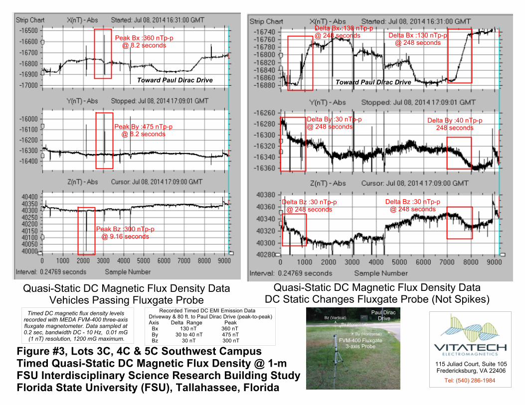
meters) from Paul Dirac Drive. Figure #3 is presented below for EMI assessment:

Quasi-Static DC Magnetic Flux Density DataVehicles Passing Fluxgate Probe

Quasi-Static DC Magnetic Flux Density DataDC Static Changes Fluxgate Probe (Not Spikes)

Figure #3, Lots 3C, 4C & 5C Southwest CampusTimed Quasi-Static DC Magnetic Flux Density @ 1-mFSU Interdisciplinary Science Research Building StudyFlorida State University (FSU), Tallahassee, Florida

Timed DC magnetic flux density levels recorded with MEDA FVM-400 three-axis fluxgate magnetometer. Data sampled at 0.2 sec, bandwidth DC - 10 Hz, 0.01 mG

(1 nT) resolution, 1200 mG maximum.

Peak Bx :360 nTp-p@ 8.2 seconds

Peak By :475 nTp-p@ 8.2 seconds

Peak Bz :300 nTp-p@ 9.16 seconds

Delta Bz :30 nTp-p@ 248 seconds


Delta By :40 nTp-p248 seconds

Delta By :30 nTp-p@ 248 seconds

Delta Bx :130 nTp-p@ 248 seconds Delta Bx :130 nTp-p

@ 248 seconds

115 Juliad Court, Suite 105Fredericksburg, VA 22406

Tel: (540) 286-1984


Bz (Vertical)

Bx (Horizontal)

By (Horizontal)

Paul Dirac Drive

Toward Paul Dirac DriveToward Paul Dirac Drive

Recorded Timed DC EMI Emission Data Driveway & 80 ft. to Paul Dirac Drive (peak-to-peak)Axis Delta Range Peak Bx 130 nT 360 nT By 30 to 40 nT 475 nT Bz 30 nT 300 nT

On the left side panel the spikes represent cars passing on driveway which are

indicated by higher peaks in the By axis facing the driveway towards the

ferromagnetic vehicles (this is due to the geomagnetic field). The moving vehicles

required 4 to 4.5 seconds to reach the peak as noted in the Bx, By and Bz axis and

about 4 to 4.5 seconds to pass to Paul Dirac Drive. The right side panels show a

scaled up version of the right panel data where the delta indicates changes in the

geomagnetic magnetic field from passing vehicles which is lower than the peak

spikes. The objective was to record the DC static and Quasi-Static DC magnetic

fields near the driveway and the National High Magnetic Field Laboratory for 36

minutes to document the environment and potential DC EMI issues.

Conclusion Static & Quasi-Static DC Magnetic Field Issues

I am very concerned with the National High Magnetic Field Laboratory on Paul

Dirac Drive directly across the street from Lots 3C, 4C and 5C. I am almost certain

(unless there is evidence to the contrary) that elevated and high magnetic field

emissions (i.e., transients, EMPs and other emission types) will emanate from the


of 22

research facility due to experiments and / or high power demands from the National

High Magnetic Field Laboratory and the nearby underground electrical distribution

feeders adjacent to Lot 3C during high current experiments. If this site is selected,

then I must meet with the Director of the National High Magnetic Field Laboratory

to discuss “containment and control” of spurious electric and magnetic field

emissions due to experiments. Furthermore, I must also record 24 to 48 hour timed

AC ELF and static/quasi-static EMI data at the proposed EMI sensitive research

laboratory locations in the future Interdisciplinary Science Research Building to

ensure optimal low levels depending on the recommended mitigation solutions such

as magnetic or electric field shielding and / or Active Compensation System (ACS)

technology. We must be absolutely certain that the future in close proximity to the

National high Magnetic Field Laboratory will not compromise the research proposed

for this new facility under any circumstances.

Moving Vehicle Quasi-Static DC Magnetic Fields

Vitatech recorded timed DC EMI data from moving vehicles at the University of

Florida future Nanotechnology Research Center in Gainesville, Florida, nearly a

decade ago. Calculated U.S. car and bus vehicle profiles were generated by

applying the decay data to Curve Fitting software. The average mass of a U.S. car

is 3,000 lbs and of a large U.S. bus is 30,000 lbs (DOT information). Comparing the

car and bus EMI emission data, the below chart presents the EMI decay rates based

upon the predicted U.S. vehicle mass formulas shown below in Table #1:

Distance Car Bus 1 m 3.50 mG 30.0 mG 6 m 0.48 mG 2.6 mG 12 m 0.22 mG 1.0 mG 18 m 0.15 mG 0.59 mG 24 m 0.11 mG 0.40 mG 30 m 0.08 mG 0.30 mG 36 m 0.07 mG 0.23 mG 40 m 0.06 mG 0.20 mG

Calculated Vehicle Profiles

Special Note: magnetic fields decay more rapidly after 30 meters than the

calculated levels indicate. Table #1, U.S. Vehicle Predicted DC EMI Emission Profile

Since the University of Florida (UF) and Florida State University (FSU) are in

reasonable close proximity, the UF vehicle data will apply to the Interdisciplinary

Science Research sites. Typically, DC magnetic interference is caused by

perturbations in the geomagnetic field of the earth from moving ferromagnetic

objects (i.e., vehicles, subways, elevators, metal carts, etc.) – something like a pebble

in the pond. These perturbations are captured by the fluxgate magnetometer and

presented as differential peak-to-peak changes in the recorded timed geomagnetic

field data. While recording the quasi-static DC data several large campus busses

and delivery trucks passed site. Therefore, I recommend at least 50 meters (164 ft.)

separation distance from all adjacent road curbs to any EMI sensitive ion beam

imaging laboratories (i.e., TEMs, SEMs, STEMs, FIBs, E-Beams, etc.) and magnetic

imaging tools (NMRs, SQUIDS, MRIs, etc.).


of 22

Predicted Elevator Recorded Quasi-Static DC Magnetic Fields

Vitatech and the University of Alberta in Edmonton, Canada, collaborated on

measuring (and quantifying by curve fitting software) the quasi-static DC magnetic

flux density level changes in magnetic flux over time (nanotesla - nTpeak-to-peak)

from a moving ThyssenKrupp passenger elevator in the Engineering Building. The

ThyssenKrupp passenger elevator specifications are as follows: Type: Overhead

Traction; Capacity: 4500 lbs.; Car Weight: 5290 lbs.; and, Counter Weight: 7540 lbs.

Vitatech shows the elevator DC EMI emission formula solved in units of milligauss

(mG) peak-to-peak as a function of distance (d) in meters from the center:

mG (passenger) = 647(d)-2.65

Table #2 shows the predicted Br resultant peak-to-peak magnetic emission profile of

the overhead traction passenger elevator recorded at the University of Alberta.

Radial distances in meters/feet from the center of the passenger elevator were

solved for six thresholds: 10 mG, 5 mG, 1 mG, 0.5 mG, 0.2 mG and 0.1 mG.

Predicted Passenger Elevator DC Emission Profile Level Distance From Center10.0 mG 4.82 m (15.8 ft.) 5.0 mG 6.27 m (20.6 ft.) 1.0 mG 11.50 m (37.7 ft.) 0.5 mG 14.94 m (49.0 ft.) 0.2 mG 21.11 m (69.3 ft.) 0.1 mG 27.42 m (89.9 ft.)

Table #2, University of Alberta Passenger Elevator DC EMI Profile

Vitatech recommends locating EMI sensitive instruments and tools at the

appropriate separation distance from the passenger elevator (add 6 meters or 20

feet for service/freight elevators) to avoid the need for DC mitigation (i.e., shielding /

active cancellation elevator or active cancellation of EMI impacted laboratory).

Radiofrequency Interference (RFI)

In the United States, the Federal Communications Commission (FCC), not the local

municipal zoning authorities or law enforcement, has legal jurisdiction over

radiofrequency interference (RFI). Simply stated, RF devices (intentional and

unintentional emitters) are not permitted to cause interference within other radio

or television services, electronic equipment and systems. At present, there are no

mandated radiofrequency interference (RFI) susceptibility government standards in

the United States. The only equipment susceptibility standards that exist are

unique to equipment (quality control) internal standards written by equipment

manufacturers based on radiated emission standards for intentional radiators set

forth by FCC. In other words, equipment manufactured within the United State

must be designed to function properly within a radiated emission field level from

intentional radiators.


of 22

In Europe, there are susceptibility (radiated immunity) standards, such as the EN

61000-6-1 states 3 V/m level for residential electronic equipment, while 10 V/m is

standard for industrial electronic equipment in the EN 61000-6-2. Engineers in the

United States utilize the European susceptibility standards as a guideline.

Vitatech recommends 3 V/m as the industrial RFI threshold and 1 V/m for the

medical/scientific instrument RFI threshold for maximum performance.

RFI Electric Field Strength Site Assessments & Conclusions

RF spectral electric field strength data in volts-per-meter (V/m) was recorded with

the SRM-3000 spectrum analyzer at the center of Lot 4B and the woods in the

center of Lots 3C and 4C along the cut path. The RFI data was collected as

sweeping samples within the spectral range of 75 MHz to 3 GHz. The RF electric

field strength data collected is presented in Diagrams #3 and #4 below:


of 22

Final RFI Conclusion: Lot 4B of Diagrams #3 and Lots 3C/4C from Diagram #4 fully

comply with the recommended 1 V/m electric field strength threshold for scientific

and medical equipment between 75 MHz to 3 GHz RF bandwidth. Vitatech also

measured from 100 kHz to 300 MHz these RFI levels also fully complied with the 1

V/m electric field strength threshold at both sites. Given that the peak electric field

strength levels were below 1 V/m from 100 kHz to 3 GHz throughout the two (2)

tested sites, Vitatech would conclude that the footprint reserved for the future

Interdisciplinary Science Research Building RF levels are acceptable for scientific

and medical instruments.

It should be noted that the typical attenuation for building construction materials

such as the below grade research EMI / RFI sensitive rooms range from -30 to -40

dB depending on the concrete thickness, types of materials, paints and other

parameters that impact the properties of reflection, absorption and transmission

besides radiated power. For example an external 1 V/m RF source would be

attenuated from 0.032 V/m to 0.01 V/m assuming -30 dB to -40 dB of attenuation

from the building due to absorption and reflection. The recorded levels at both

sites were less than 0.1 V/m, and the future Interdisciplinary Science Research

building levels would be attenuated down to 0.003 V/m to 0.001 V/m.

Construction Recommendations

It is absolutely critical that a well-qualified, highly skilled electrical contractor with

licensed electricians be selected to perform the electrical installation work. The

electrical contractor must test every neutral (feeders, branch and lighting

circuits) in the building during construction to guarantee electrical

isolation from the grounding system. The neutral-grounding system isolation

test must be documented and submitted to the EMI Consultant for review. If the

electrical distribution system is fully compliant with the N.E.C., then there will be

minimal circulating ground currents except due to leakage currents (i.e.,

transformers, refrigerator compressors, etc.) returning along the various conductive

paths and a steel frame and/or concrete reinforced building with uncoated steel

rebar back to the switchgear room ground bonding point and/or to the primary

building transformer grounds. Nevertheless, Vitatech recommends fiberglass rebar

in the concrete slabs of all EMI sensitive research tools to guarantee that any

returning ground currents do not travel beneath the tools. Vitatech highly

recommends that all electrical contractors follow the Required Practices for

Mitigating AC ELF Magnetic Fields:

Required Practices for Mitigating AC ELF Magnetic Fields

1) Each single phase circuit, including all lighting circuits, must have a

dedicated neutral with each phase to ensure maximum magnetic field

cancellation along the conduit paths.

2) All neutral conductors must be tested for unintentional grounding – final

testing report must be submitted to the EMI Consultant for review.

3) In EMI sensitive areas, including the hallways, all circuit conductors

(phases, neutral and any grounding) must be twisted for maximum


of 22

magnetic field cancellation. It is recommended to use nylon wire ties in

switchboards, pull boxes, wire-ways, surface metal raceways and

equipment to minimize conductor separation in the EMI sensitive research

areas.

4) Do not route any circuits (power, signal or telecommunications) above or

below EMI sensitive laboratories, except those circuits required for the

specific use of the laboratory. All conduits (power, signal or

telecommunications) must travel in the center hallway ceiling (none should

be below the laboratory floor providing the maximum separation distance

from future EM tool column and power conduits. All branch and lighting

circuits must have dedicated neutrals that follow each phase conductor.

5) All primary feeders within 50 feet and inside of the building must be in

RGS conduits. All 480//277V and similar high current feeders within 50

feet and inside of the building must be shielded. Twisting the phase and

neutral conductors will also decrease the magnetic field emission profiles.

6) Electrical equipment should not be located within 16.4 feet (5 meters) of

the EMI sensitive tool columns or instruments. Electrical feeders 100 amps

and higher must be shielded and routed to ensure maximum separation

distance from the EMI sensitive tools.

7) Vitatech does not recommend the use of busways of any size in scientific

and research building unless the busway EMI emissions are simulated and

the appropriate distance to EMI sensitive tools defined. If busways are

specified, it will be necessary to install magnetic shielding systems around

the electrical room walls to attenuate the magnetic field emissions in

adjacent EMI sensitive laboratories and offices.

Electrical Room 60 Hz EMI Emissions

Typically, Vitatech recommends at least 5 meters of separation distance between

unshielded electrical rooms and 20 meters from unshielded Main Switchgear Rooms

to EMI sensitive research areas and laboratories.

Doors & Hardware Options For EM & TEM Rooms Extremely Important

Vitatech recommends non-ferrous and/or wooden doors where possible to minimize

the DC EMI impact. Doors will have a minimal EMI impact on EM tools if they are

composed of nonferrous materials such as aluminum or wood. A glass door with a

steel frame is acceptable in clean rooms. Aluminum and/or wooden doors are

acceptable for imaging laboratories with steel hinges and locking hardware. Special

non-ferrous doors should not be fabricated unless within 6 meters of any EMI

sensitive tools. Therefore, using steel hardware (only hinges and locks) is

acceptable in non-ferrous doors for security and safety, and therefore should not

present a serious EMI impact. The University of Alberta study examined the

impact of steel doors on DC EMI magnetic field emissions and concluded as follows

The effect of moving metallic objects in the Earth’s geomagnetic field were

observed to significantly perturb magnetic field levels. Specifically, (steel)

doors were found to perturb magnetic field levels above the acceptable range of


of 22

5 nT over distances as great as 6m. It is recommended to keep (steel) doors

away from sensitive areas by at least 6m, and if possible, 12m to be safe. It

was found that a measurable difference in the functional behavior of the fall-

off of the magnetic field perturbations existed between rebar reinforced

concrete structures and steel frame structures. Specifically, it was observed

that perturbations in steel frame structures, both due to doors and elevators,

fell off more rapidly than in reinforced concrete structures. This was

attributed to a higher concentration of steel in steel frame structures which

essentially tended to shield the perturbations.

Concrete Verses Steel Building Structural Frame Discussion

In all building types, the circulating ground currents due to electrical code

violations (i.e., grounded neutrals, wiring errors, etc.) in the electrical distribution

system traveling on the conductive steel structures such as rebar, steel beams, and

metallic pipe/duct systems generate the most serious EMI problems for high

resolution imaging tools (i.e., STEMs, SEMs, TEMs, FIBs, E-Beams, NMRs, MRIs,

etc.). These conductive paths are part of an unintentional electrical circuit for

ground currents seeking a return path to the secondary grounded-wye of the source

transformer.

A ground current of 1 amp on a conductive path (steel rebar and/or steel beam) will

generate a magnetic field of 2 mG at one-meter separation distance that diminishes

at a linear decay rate (1/r in meters) from the conductive path according to the

following formula:

B rms = 2(I in amps)/r in meters

But why should a new code-compliant high-tech building with a well inspected

electrical distribution system have circulating ground currents? Not easy to answer

-- but simply stated -- if there are electrical code violations (i.e., grounded neutrals,

wiring errors, etc.) in the low-voltage electrical distribution system, then circulating

ground currents will return via the steel rebar and building steel presenting a

possible AC ELF EMI problem in the EMI sensitive Imaging Areas and Cleanroom

tool areas.

In concrete buildings, steel rebar is used to reinforce the vertical columns and

horizontal floor slabs of the structure. Since the steel rebar in the columns and floor

slabs are tied together with metal wire before the concrete is poured, the building

frame is essentially a continuous metallic structure similar to a steel building, but

with significantly higher resistive impedance (steel buildings are lower impedance

structures by nature of the interlocking, bolted and welded steel frame). There are

several types of rebar that can be used as reinforcement: uncoated steel, epoxy

coated, non-magnetic stainless steel and fiberglass. Uncoated steel rebar is used in

most building construction except where salt intrusion can corrode and compromise

structural integrity, then epoxy coated rebar is more effective. In recent years,


of 22

several research facilities have been constructed using epoxy coated rebar to

minimize circulating ground currents inside the reinforced columns and slab.

First, let's discuss the use of epoxy coated reinforcing steel in the slab on grade --

although the epoxy coating will theoretically minimize ground current circulation

on the steel rebar, there are still issues regarding electromagnetic induction and

magnetic flux reticulating along the steel rebar path beneath the tool from time-

varying DC and AC magnetic fields. A simple solution is to replace the steel rebar

in the on grade concrete floor slabs with fiberglass reinforcement (does not apply to

columns and floors not on grade): now potential DC and AC EMF EMI emissions

problems are eliminated inside the imaging rooms beneath the tool, but this only

works for on-grade slabs.

Achieving less than 1 mG down to 0.01 mG peak-to-peak in the Imaging Areas is

the real objective and depends on the magnitude of the magnetic emission source

(time-varying AC or DC magnetic flux), polarization of the field (direction) and the

permeability of the steel rebar plus the influence (mutual inductance, etc.) of other

nearby ferromagnetic objects. A local time-varying AC ELF magnetic field source

(i.e., primary/secondary feeders, transformers, electric panels, distribution

transformers, conduits, etc.) will induce magnetic fields (electromagnetic induction)

in any nearby ferromagnetic materials (steel rebar, I-beams, etc.) generating an

opposing AC ELF magnetic field (Lenz's Law) in the steel rebar from the localized

external electromagnetically induced time-varying source, which is usually small in

size compared to the magnetically coupled steel rebar frame. The AC ELF EMI

induced fields are localized and rapidly diminish from the inducing source.

Therefore, circulating ground currents due to electrical code violations in the

electrical distribution system traveling on conductive return paths such as uncoated

rebar and building steel present the greatest EMI threat to sensitive imaging tools,

not the magnetically induced time-varying currents within the ferromagnetic

materials from nearby electrical sources (the difference is very important).

An EMI Study performed by the University of Alberta and Vitatech Engineering

examined the response of steel rebar to DC induced magnetic fields and circulating

ground currents – the following Conclusion was presented:

Rebar was investigated to determine if it coupled magnetic fields. It was

found to be ferromagnetic. That it becomes permanently magnetized is not a

serious problem… The rebar does, however, couple strongly with the magnetic

field along its length. Again, this does not pose a significant problem, as it

was also found that field levels fall off exponentially from the end of the rebar.

So long as a reasonable distance (minimum of 1m, preferably 2m) is

maintained between rebar and sensitive areas, the coupling is likely not to be

a concern. It was also found that rebar is highly conductive, which may pose

a significant problem in the future, if net currents are to develop in them. In

this case, a ground current flowing along the rebar would only fall off as 1/r,

and hence may cause serious problems. Based on these measurements, it can


of 22

be concluded that rebar may not cause problems with magnetic field levels as

demonstrated in the shielding effect of rebar reinforced concrete structures and

steel frame structures, and the exponential decay of the coupling of a magnetic

field along its length, however, care should be exercised in using rebar due to

its high conductivity that may cause problems in the future.

However, the University of Alberta study discovered DC EMI differences caused by

moving elevators and doors in concrete reinforced and steel frame buildings, which

are presented in the same Conclusion:

The effects of moving metallic objects in the Earth’s geomagnetic magnetic

field were observed to significantly perturb magnetic field levels. Specifically,

doors were found to perturb magnetic field levels above the acceptable range of

5nT over distances as great as 6m. It is recommended to keep doors away

from sensitive areas by at least 6m, and if possible, 12m to be safe. Elevators

were also found to significantly perturb magnetic field levels. It was found

that to reach 5nT, distances as great as 38m had to be achieved. It is

recommended that elevators be kept as far away as possible, at least 38m, and

if possible, further to be safe. It was found that a measurable difference in the

functional behavior of the fall-off of the magnetic field perturbations existed

between rebar reinforced concrete structures and steel frame structures.

Specifically, it was observed that perturbations in steel frame structure, both

due to doors and elevators, fell off more rapidly than in reinforced concrete

structures. This was attributed to a higher concentration of steel in steel

frame structures which essentially tended to shield the perturbations.

According to the University of Alberta study, the DC EMI emissions inside steel

frame buildings caused by moving ferromagnetic objects (i.e., elevators, doors and

vehicles) were lower because the thick steel beams appear to provide shielding (or

rather absorb more magnetic flux) compared to the reinforced concrete steel.

However, there is an EMI AC ELF emission higher risk from circulating ground

currents in a steel frame building and uncoated steel rebar building than in an

epoxy coated steel rebar reinforced concrete building. Therefore, the basement

level TEM suites should use fiberglass reinforced rebar, not steel or epoxy coated

rebar, to eliminate circulating ground currents under the tools over the life of the

building. Steel rebar and/or steel beams can be used in the columns; however, using

epoxy coated rebar for the columns would minimize circulating ground currents in a

reinforced concrete structure. Unfortunately, during construction the epoxy

insulation on the coated rebar can be compromised as installed and formed, so each

section must be tested for electrical isolation to minimize conductive paths ensuring

compliance (Quality Control Issue), which is very time consuming.

In conclusion, the DC magnetic emissions from moving ferromagnetic objects (i.e.,

elevators, vehicles and other objects) appear to emanate further in concrete

reinforced building with steel rebar (epoxy coated or uncoated) rather than in steel

frame building according to the University of Alberta study. However, circulating


of 22

ground current AC ELF magnetic emissions due to electrical code violations in the

electrical system would travel along the low impedance path of the steel frame

structure, and to a lesser effect, on the higher impedance uncoated steel rebar

structure, back to the source transformer wye grounded neutral point (usually the

415/240 V source). An epoxy coated rebar structure field tested for electrical

isolation would not permit return ground currents to return inside the structure;

however, the ground return currents would return on the metal conduits, pipes,

HVAC ducts, unistrut supports and any other conductive paths back to the main

building grounds.

Therefore, it is critical that a well-qualified, highly skilled electrical contractor with

licensed electricians be selected to perform the electrical installation work. The

contractor should test every neutral (feeders and branch circuits) in the building

during construction to guarantee electrical isolation from the grounding system. If

the electrical distribution system is fully compliant with the electrical code, then

there will be very low circulating ground currents typically caused by leakage

currents returning along the various conductive paths and a steel frame and/or

concrete reinforced building with uncoated steel rebar would have very similar AC

EMI effects on the nearby high resolution imaging tools.

Additional Comments Using Metal Rebar Beneath TEM Imaging Labs

Vitatech typically recommends the use of carbon fiber rebar or fiberglass fill under

EM Imaging Areas rather than non-magnetic stainless steel (very expensive) and/or

epoxy coated rebar to avoid circulating ground currents on stainless steel or rebar

directly below EMI sensitive research tools.

However, epoxy coated rebar can be used in the EM inertia slabs and concrete

under slabs as long as the epoxy coating is not compromised during installation and

all the epoxy coated rebar is electrically isolated (verified by on-site continuity

testing) from the other epoxy coated rebar and electrically isolated from any steel

rebar and grounding system in the building so ground/net currents cannot travel on

the epoxy coated rebar beneath the EM tools compromising the image quality from

ground current magnetic field emissions. The EM shielded floor shield should be

located beneath the EM inertia slabs to avoid transferring vibrations into the

inertia slabs and EM tool. However, Vitatech prefers the use of fiberglass fill and/or

carbon fiber rebar in the concrete spaces directly beneath EM tools to completely

eliminate any potential EMI problems with circulating currents on electrically

compromised epoxy coated rebar due to nicks in the epoxy coating or unknown

problems that compromised electrical isolation occurred during construction. It

should be noted that epoxy coated non-magnetic stainless steel (Grades 310 and 316

only) rebar has the same electrical isolation challenges as epoxy coated rebar, not

magnetic and significantly more costly than epoxy coated steel rebar (Vitatech does

not recommend this as a solution unless cost is not an issue). Finally, DC magnetic

field magnetization due to moving steel rebar and epoxy coated steel rebar with

electromagnets in the mill and transport will not seriously impact the EM tools and

can shimmed into calibration during tool calibration.


of 22

Non-magnetic stainless steel, also known as austenitic, has very low magnetic

permeability and almost no response to a magnet when in the annealed condition.

However, when these steels have been cold worked by wire drawing, rolling or even

center less grinding, shot blasting or heavy polishing the non-magnetic properties

change. After substantial cold working, Grade 304 may exhibit a strong response to

a magnet, whereas Grades 310 and 316 will in most instances still be almost totally

non-responsive. In general, the higher the nickel-to-chromium ratio the more stable

is the austenitic structure and the less magnetic response that will be induced by

cold work. Therefore, Vitatech does not normally recommend using non-magnetic

stainless steel unless it can be guaranteed to be the non-magnetic grade, which also

requires field testing all pieces with a fluxgate magnetometer to ensure using the

non-magnetic grade before installation.

Metal Stud Framing & PVC Conduit Discussion

Metal stud framing and metal conduits can present an AC ELF EMI problem when

circulating ground currents due to electrical code violations (i.e., grounded neutrals,

wiring errors, shorts, etc.) are present in the electrical distribution system and

travel on the steel stud walls and metal conduits adjacent to sensitive imaging

suites. Several research facilities such as Oak Ridge National Labs, Duffield Hall

(Cornell University) and Argonne National Labs (SAMM Building) have used

wooden studs and PVC conduits with twisted conductors in the high resolution

imaging labs to minimize potential DC and AC ELF EMI problems. It should be

noted that the Argonne SAMM Building is located more than 100 meters from the

nearest road and any elevators to minimize quasi static DC EMI problems. The

University of Sydney AIN Building is located in the center of a busy campus

surrounded by multiple access roads and a freight elevator within an affective

proximity of the Imaging Area and sensitive instrument locations. Furthermore, the

predicted DC EMI data near selected imaging labs will directly vary with the

elevator and adjacent traffic emissions so it is not possible to have a pristine DC EMI

environment like the SAMM site. Therefore, wooden stud framing will not benefit

the EM labs. Also, Vitatech does not recommend PVC conduits in EM tool rooms

because the electrical code in the United States requires metal conduits to be code

compliant and there is a potential liability issue if someone is accidently

electrocuted. The EMI advantage using PVC conduits is minimal and not worth the

risk. Vitatech recommends metal conduit with twisted conductors for low current

circuits under 100 amps in the Imaging Labs. The client must issue a “hold

harmless” if PVC conduits and twisted conductors are recommended for the Imaging

Areas.

Time-Varying AC ELF & Quasi-Static DC Mitigation Strategies

Eliminating AC ELF (power frequency) and quasi-static DC magnetic field

emissions is challenging due to the plethora of primary / secondary sources,

underground feeders, adjacent buildings, and even the support equipment for tools

themselves. However, reducing the magnetic field levels to acceptable (optimal

performance) levels for specific instruments can be accomplished through a variety

of tactics.


of 22

First and foremost, it is critical that separation distance be viewed as the primary

method to providing the best EMI environment for a sensitive tool. Placing

instruments and labs away from AC ELF power frequency and quasi-static DC (i.e.,

roads with moving vehicles, loading docks, elevators, etc.) sources is not only

suggested but encouraged, provided it is an available option for a specific site. This

includes providing the greatest distance between the instrument and the following:

transmission lines, underground feeders, transformers, electrical rooms, electrical

panels, electrical equipment and roads, train tracks, subways (both above and below

grade), elevators, roads, loading docks, parking garages, etc. How much separation

distance is required is dependent upon two factors: the nature of the surrounding

sources, and the EMI sensitivity of the instrument.

After all reasonable solutions regarding applicable separation distance have been

exhausted and/or considered, there are two methods for reducing magnetic field

levels within an area.

The second and most effective method to attenuate time-varying 60/50 Hz and

higher harmonic magnetic fields within a microscopy lab is to design and install a

six-sided AC ELF (3 Hz to 3000 Hz) magnetic shielding system composed of highly

conductive, seam welded thick aluminum plates. This is the preferred solution

when elevated AC ELF magnetic fields up to 6 mG p-p must be attenuated down to

very low 0.1 mG p-p (10 nT p-p) and less levels in the Bx, By and Bz axis measured

at the tool column as required for TEMs and STEMs from circulating ground/net

currents due to N.E.C. violations (i.e., grounded neutrals, wiring errors, etc.) in the

electrical distribution system and traveling on conductive metallic paths (i.e.,

water/gas pipes, HVAC ducts, metal studs, etc.).

Attenuating the impact from quasi-static magnetic field sources (i.e., elevators,

traffic, trains, subways, etc.), DC magnetic shielding is applied on six-sides to lower

the ambient geomagnetic fields at the column which enhances the overall

performance of DC ACS systems (see next paragraph for details). Magnetic

shielding can be implemented in one of two ways: by shielding the source itself (i.e.,

shielding an electrical room), or by shielding the instrument or room housing the

instrument (i.e. shielding an entire lab). The method recommended for a location

depends on the sources surrounding the area and sizes of the labs, but multiple

factors determine the proper shielding recommended for any instruments.

Shielding of the utilities (i.e., primary feeders, substation vaults, etc.) is indeed

possible, but will require an advanced knowledge of the physical locations of the

conduits (and preferably, the current on each circuit) to ensure proper mitigation is

enabled.

The third method to mitigate AC ELF and quasi-static DC magnetic field emissions

is the application of active compensation system (ACS) technology. As the name

suggests, ACS technology actively senses the incident magnetic field at the tool

column where the fluxgate magnetometer probe is located, sending the Bx, By and

Bz magnetic field signal to the ACS processor that generates an equal and opposite


of 22

(180 degree) magnetic field signal. The Bx, By and Bz magnetic signals are

amplified and supplied to six (6) orthogonal Helmholtz coils installed around the

tool or room with one loop pair per axis canceling the incident magnetic field

emission, thus attenuating the magnitude of the magnetic field at the tool column.

This is especially pertinent to areas with traffic surrounding the site on all sides (for

example, Engineering Building #4 upon UCLA’s campus). This method has its

limitations due to the ACS response times, number of external EMI sources and other

challenges that impact the overall attenuation characteristics and performance, so

selecting the proper model, manufacturer and installation solution (i.e., coils around

the room vs. the tool) is absolutely essential for optimal ACS performance.

Vitatech has successfully designed and installed AC ELF, DC and quasi-static DC

magnetic shielding and RF shielding systems for research, medical and engineering

facilities in the United States and around the world. We will design and

recommend the most cost-effective mitigation solutions for EMI/RFI sensitive

research tools for this project based upon more than 20 year of professional

experience.

AC ELF, DC & RF Test Instruments

FieldStar 1000 Gaussmeter - AC ELF Magnetic Flux Density

Vitatech recorded the AC ELF magnetic flux density data using a FieldStar 1000

gaussmeter with a NIST traceable calibration certificate manufactured by Dexsil

Corporation. The FieldStar 1000 has a resolution of 0.04 mG in the 0 - 10 mG

range, 1% full-scale accuracy to 1000 mG and a frequency response of 60 Hz (55 - 65

Hz @ 3dB). Three orthogonal powdered-iron core coils are oriented to reduce

interference to less than 0.25% over the full dynamic range. The three coils are

arranged inside the unit holding horizontal with the display forward: Bx horizontal

coil points forward, By horizontal coil points to the right side, and Bz vertical coil

points upward. The microprocessor instantly converts the magnetic field to true

RMS magnetic flux density (milligauss) readings of each axis (Bx, By, Bz) and

simultaneously calculates the resultant Rrms (root-means-square) vector according

to the following formula:

When collecting contour path data, a nonmetallic survey wheel is attached to the

FieldStar 1000 gaussmeter and the unit is programmed to record mapped magnetic

flux density data at selected (1-ft., 5-ft., 10-ft. etc.) intervals. The FieldStar 1000 is

exactly 39.37 inches (1 meter) above the ground with the survey wheel attached.

Along each path the distance is logged by the survey wheel and the relative

direction (turns) entered on the keyboard. Up to 22,000 spot, mapped and timed

data points can be stored, each containing three components (Bx, By & Bz), event

markers and turn information. After completing the path surveys, magnetic flux

density data is uploaded and processed. All plots display a title, time/date stamp,

ID path number, and the following statistical data (in milligauss) defined below:

R Bx By Bzrms = + +2 2 2


of 22

Peak - maximum magnetic field (flux) value measured in group.

Mean - arithmetic average of all magnetic field (flux) values collected.

The following is a quick description of the Hatch, Profile and 3-D Contour plots

presented in the figures of this report:

Hatch Plot - data is represented by four difference hatch marks (0.1 mG,

0.25 mG, 0.5 mG and 1.0 mG thresholds) based on width and color as a

function of distance along the survey path that shows 90 and 45 degree turns.

Note: the site drawing and all Hatch Plots were scaled in feet to verify actual

recorded distances and correct survey locations.

Profile Plot - data shows each recorded component (Bx, By, Bz) axis and the

resultant (Br) levels as a function of distance: Bx (red) is the horizontal

component parallel to the survey path, By (green) is the horizontal

component normal (perpendicular) to the survey path, and Bz (blue) is the

vertical component with the computed Br resultant RMS (root-means-square)

summation of the three components.

3-D Contour Plot - displays the magnitude of the computed resultant Br in

the vertical direction (peaks and valleys) using eight threshold color ranges

from 0.1 to 2-mG. Letter markers are included on the 3-D Plots to reference

turns on the Hatch Plots.

MEDA FVM-400 DC Three-Axis Magnetometer

timed three-axis DC magnetic flux density levels were recorded from the elevators

and moving vehicles with a three-axis fluxgate magnetometer at 1 second intervals

over a 10-minute periods. The MEDA FVM-400 three-axis fluxgate magnetometer

has 1 nT (0.01 mG) resolution and 1.2 Gauss (1,200 mG) maximum range with 1%

full scale accuracy from 0-10 Hz. Data is downloaded directly to a computer during

data collection and processed for graphical presentations.

SRM-3000 RF Spectrum Analyzer - Electric Field Strength Data 100 kHz - 3 GHz

The state-of-the-art SRM-3000 Spectrum Analyzer is a radio-frequency (RF) electric

field strength meter for broadband measuring and monitoring from 100 kHz to 300

MHz with a single axis active antenna and 75 MHz to 3 GHz with an isotropic

active antenna. Each antenna attached to the top of the device records spectral

data in Volts-per-meter (V/m) and simultaneously visually arranges it for

immediate use. It records average, maximum and peak data while recording each

of its timed “samples” at an average rate of 1 sample per second. In addition, safety

analyses can be performed, which record the RF electric field strength levels in

comparison to the recommended exposure limits expressed in percentile ratio.

This completes the EMI/RFI Site Survey Report – Florida State University

Interdisciplinary Science Research Building Recommendations and Mitigation

Strategies. The contents of this report are intended for the exclusive use of the

Florida State University and Wilson Architects.


of 22

Best regards,

Louis S. Vitale, Jr.

Chief Engineer & Founder

Attachments: Figures #1 - #3 (total of four figures)

Br Bx

By Bz

Distance in feet

0 100 200 300 400 500 600

0

2

4

6

8

10

12

14 2 2 2 2 2Rec 35 File FSU1 Taken 7/8/14 ID-3B L1PEAK = 13 mG, MEAN = 2.97 mG

Profile Plot

Eng

inee

r Driv

e

13 mG PeakCenter ConductorThree (3) 230 kV

Transmission Lines

Br Bx

By Bz

Distance in feet

0 200 400 600 800 1000 1200

0

2.5

5

7.5

10

12.5

15

17.5

20

22.5 2 2 2 2 2 2 2 2 2 2 2

Rec 36 File FSU1 Taken 7/8/14 ID-3B L2PEAK = 20.4 mG, MEAN = 1.85 mG

Profile Plot

Engineer Drive

Br Bx

By Bz

Distance in feet

0 100 200 300 400 500 600 700 800

0

2.5

5

7.5

10

12.5

15

17.5

20

22.5 2 2 2 2Rec 38 File FSU1 Taken 7/8/14 ID-3B L4

PEAK = 21.7 mG, MEAN = .496 mG

Center ConductorTwo (2) 230 kV

Transmission Lines

0.04 mG RMS

Red Markers

A BLevy Ave

Bush/T

ree

Are

a

Grassy Area

Eng

inee

r D

rive

A

1 mG RMS (3 mGp-p)

1 mG RMS (3 mGp-p)

1 mG RMS (3 mGp-p)1.0

B

Start

Start

Start

End

End

End

.1 < < .5 < < 1 < < 5 < (Br in mG)

Hatch Plot

Rec 36 File FSU1 Taken 7/8/14 ID-4B L2PEAK = 20.4 mG, MEAN = 1.85 mG

Rec 35 File FSU1 Taken 7/8/14 ID-4B L1

PEAK = 13 mG, MEAN = 2.96 mG

.1 < < .5 < < 1 < < 5 < (Br in mG)

Hatch Plot

0100 200 300Distance In Feet

Start

End

EndEnd

Start

Start

.1 < < .5 < < 1 < < 5 < (Br in mG)

Rec 38 File FSU1 Taken 7/8/14 ID-4B L4

PEAK = 21.7 mG, MEAN = .497 mG

Hatch Plot

SUBSTATION

AB

A

B

1

1.0

0.16 mG RMS

0.24 mGRMS

Bush/Tree Area

0.32 mGRMS

0.2 mGRMS

0.12 mGRMS

21.7 mG RMSUnderground

Feeder

Red Markers

0.88 mGRMS

0.64 mGRMS

0.04 mGRMS

0.04 mGRMS

Figure #1, Lot 4B, Southwest CampusHatch & Profile Laterals - Magnetic Flux Density @ 1-mFSU Interdisciplinary Science Research Building StudyFlorida State University (FSU), Tallahassee, Florida

All magnetic flux density datarecorded with a FieldStar 1000gaussmeter and survey wheel

Magnetic flux density B in units of Tesla or Gauss can be specified in one of three magnetic flux density terms: B rms, B peak-to-peak(B p-p) and B peak (Bp) according to the following conversion formula:

BBp p Bp

rms= − =2 2 2

Magnetic field strength (A/m) in SI units can be convertedto units of milligauss (mG) according to the following conversion formula:

mG = 4 (X A/m)

SI & CGS Unit Conversion ChartMagnetic Flux Density

Tesla (T): 1 T = 10,000 Gauss (G)milliTesla (mT): 1 mT = 10 Gauss (G)microTesla (uT): 1 uT = 10 milliGauss (mG)nanoTesla (nT): 1 nT = 0.01 milliGauss (mG)






Tel: (540) 286-1984

Bx

By

Bz (vertical)

Gau

ssm

ete

r

Survey WheelPath Direction - Bx

Bx

By

Bz (vertical)

Gauss

mete

r


Bx

By

Bz (vertical)

Gaussm

ete

r


<0.04 mG RMSNo Hatch Marks

Levy AvenueE

ngin

eer

Drive

Rec 5 File FSU3 Taken 7/11/14 ID-S2 L2APEAK = 20.7 mG, MEAN = 1.26 mG

.1 < < .5 < < 1 < < 5 < (Br in mG)

Hatch Plot

Hatch Plot

.1 < < .5 < < 1 < < 5 < (Br in mG)

Rec 6 File FSU3 Taken 7/11/14 ID-S2 L2BPEAK = 32.6 mG, MEAN = 6.93 mG

Start

End

Start End

Hatch Plot

Rec 8 File FSU3 Taken 7/11/14 ID-S2 P1APEAK = 25.6 mG, MEAN = 10.8 mG

.1 < < .5 < < 1 < < 5 < (Br in mG)

Start

End

.1 < < .5 < < 1 < < 5 < (Br in mG)

Rec 3 File FSU2 Taken 7/10/14 ID-S2 P3PEAK = 22.7 mG, MEAN = 2.5 mG

Hatch Plot

Start

End

Start

End

.1 < < .5 < < 1 < < 5 < (Br in mG)

Rec 9 File FSU3 Taken 7/11/14 ID-S2 S1APEAK = 20.4 mG, MEAN = 2.81 mG

Hatch Plot

.1 < < .5 < < 1 < < 5 < (Br in mG)

Rec 40 File FSU1 Taken 7/8/14 ID-3C L5

PEAK = 5.96 mG, MEAN = 1.55 mG

Hatch Plot

End

Start

Figure #2, Lots 3C, 4C & 5C Southwest CampusHatch Laterals - Magnetic Flux Density @ 1-mFSU Interdisciplinary Science Research Building StudyFlorida State University (FSU), Tallahassee, Florida


BBp p Bp

rms = − =2 2 2


mG = 4 (X A/m)






Tel: (540) 286-1984

Tra

nsm

issio

n L

ine R

OW

Tra

ns

mis

sio

nL

ine

RO

W

ElectricalSubstation


Underground DistribuitionLine Along Street / Curb

Paul D

irac

Drive

Underground Distribuition


Und

erg

rou

nd

D

istr

ibu

itio

n

Profile Plots Refer To Figure #2A.

MEDA FVM-400Fluxgate GaussmeterQuasi-Static DC Data

Br Bx

By Bz

Distance in feet

0 100 200 300 400 500

0

2.5

5

7.5

10

12.5

15

17.5

20

22.52 2 2

Rec 5 File FSU3 Taken 7/11/14 ID-S2 L2A


Br Bx

By Bz

Distance in feet

0 100 200 300 400 500 600 700 800

0

5

10

15

20

25

30

35 2 2 2 2 2

Rec 6 File FSU3 Taken 7/11/14 ID-S2 L2B


Figure #2A, Lots 3C, 4C & 5C Southwest CampusProfile Laterals - Magnetic Flux Density @ 1-mFSU Interdisciplinary Science Research Building StudyFlorida State University (FSU), Tallahassee, Florida


BBp p Bp

rms = − =2 2 2


mG = 4 (X A/m)




Tel: (540) 286-1984

Br Bx

By Bz

Distance in feet

0 20 40 60 80 100 120 140

0

1

2

3

4

5

6 2 2Rec 40 File FSU1 Taken 7/8/14 ID-3C L5PEAK = 5.96 mG, MEAN = 1.58 mG

Rec 5 File FSU3 Taken 7/11/14 ID-S2 L2APEAK = 20.7 mG, MEAN = 1.26 mG

.1 < < .5 < < 1 < < 5 < (Br in mG)

Hatch Plot

Hatch Plot

.1 < < .5 < < 1 < < 5 < (Br in mG)

Rec 6 File FSU3 Taken 7/11/14 ID-S2 L2BPEAK = 32.6 mG, MEAN = 6.93 mG

Start

End

Start End

Hatch Plot

Rec 8 File FSU3 Taken 7/11/14 ID-S2 P1A


.1 < < .5 < < 1 < < 5 < (Br in mG)

Start

End

.1 < < .5 < < 1 < < 5 < (Br in mG)

Rec 3 File FSU2 Taken 7/10/14 ID-S2 P3PEAK = 22.7 mG, MEAN = 2.5 mG

Hatch Plot

Start

End

Start

End

.1 < < .5 < < 1 < < 5 < (Br in mG)

Rec 9 File FSU3 Taken 7/11/14 ID-S2 S1APEAK = 20.4 mG, MEAN = 2.81 mG

Hatch Plot

.1 < < .5 < < 1 < < 5 < (Br in mG)

Rec 40 File FSU1 Taken 7/8/14 ID-3C L5


Hatch Plot

End

Start



Tra

ns

mis

sio

n L

ine

RO

WT

ran

sm

iss

ion

Lin

e R

OW

ElectricalSubstation


Underground DistribuitionLine Along Street / Curb

Pau

l Dira

c

Drive



Un

de

rgro

und

D

istr

ibu

itio

n

Hatch Plots Refer To Figure #2.

Br Bx

By Bz

Distance in feet

0 100 200 300 400 500 600 700 800

0

2.5

5

7.5

10

12.5

15

17.5

20

22.5

25 2Rec 3 File FSU2 Taken 7/10/14 ID-S2 P3


Bz Vertical FieldGround/Net CurrentDistribution System

Paul DiracDrive

UndergroundDistribution Line

13 mG PeakSpot

Center ConductorThree (3) 230 kV

Transmission Lines

0.04 mG RMS

1 mG RMS (3 mGp-p)Start





Bx

By

Bz (vertical)

Gaussm

ete

r


Start

Start

Start

End

End

End



20.7 mG RMSPeak Spot


End

Paul Dirac Drive



Dri

ve

wa

y

Bx

By

Bz (vertical)

Ga

ussm

ete

r


Bx

By

Bz (vertical)

Gaussm

ete

r


ParkingLot

0.04 mG RMS

Intersecftion Records 5 & 6

Intersecftion Records 5 & 6


0.12 mG RMS

0.12 mG RMS



Quasi-Static DC Magnetic Flux Density DataVehicles Passing Fluxgate Probe

Quasi-Static DC Magnetic Flux Density DataDC Static Changes Fluxgate Probe (Not Spikes)

Figure #3, Lots 3C, 4C & 5C Southwest CampusTimed Quasi-Static DC Magnetic Flux Density @ 1-mFSU Interdisciplinary Science Research Building StudyFlorida State University (FSU), Tallahassee, Florida

Timed DC magnetic flux density levels recorded with MEDA FVM-400 three-axis fluxgate magnetometer. Data sampled at 0.2 sec, bandwidth DC - 10 Hz, 0.01 mG

(1 nT) resolution, 1200 mG maximum.

Peak Bx :360 nTp-p@ 8.2 seconds

Peak By :475 nTp-p@ 8.2 seconds

Peak Bz :300 nTp-p@ 9.16 seconds



Delta By :40 nTp-p248 seconds

Delta By :30 nTp-p@ 248 seconds

Delta Bx :130 nTp-p@ 248 seconds Delta Bx :130 nTp-p

@ 248 seconds


Tel: (540) 286-1984


Bz (Vertical)

Bx (Horizontal)

By (Horizontal)

Paul Dirac Drive

Toward Paul Dirac DriveToward Paul Dirac Drive

Recorded Timed DC EMI Emission Data Driveway & 80 ft. to Paul Dirac Drive (peak-to-peak)Axis Delta Range Peak Bx 130 nT 360 nT By 30 to 40 nT 475 nT Bz 30 nT 300 nT

diagram #1, lot 4b, lots 2c, 4c & 5c with 230 kv

Documents