1

Diagnostic Evaluation of Ozone Production and Horizontal Transport in a Regional Photochemical Air Quality Modeling System

James M. Godowitcha*, Robert C. Gilliama, S.Trivikrama Raoa

aAtmospheric Modeling and Analysis Division, National Exposure Research Laboratory

Office of Research and Development, U.S. Environmental Protection Agency Research Triangle Park, NC 27711 USA

* Corresponding author address. James Godowitch, U.S. Environmental Protection Agency (E243-04), 4930 Page Rd., Durham, NC, 27703, USA Tel: +1 919 541 4802, Fax: +1 919 541 1379, E-mail: godowitch.james@epa.gov

2

Abstract

A diagnostic model evaluation effort has been performed to focus on photochemical

ozone formation and the horizontal transport process since they strongly impact the

temporal evolution and spatial distribution of ozone (O3) within the lower troposphere.

Results from the Community Multiscale Air Quality (CMAQ) modeling system are

evaluated against surface and upper-air measurements from field studies during

summer 2002 when several high O3 episodes occurred in the eastern United States.

Modeled O3 and winds are compared to research aircraft measurements and wind

profiler data, respectively, to investigate whether model underestimates of daily

maximum 8-h ozone concentrations during high O3 episodes might be attributable to

discrepancies in either or both of these modeled processes. Comparisons of 10 AM

surface O3 concentrations, which are representative of O3 levels in the residual layer

aloft, revealed that model underestimation was greater at higher observed ozone levels.

Mid-morning vertical ozone profiles corroborated this surface-level finding, as modeled

concentrations tended to be lower than observed O3 aloft. Net ozone production

efficiency (OPE) results suggested photochemical ozone formation was comparable

between the model and observations with composite OPE values of 6.7 and 7.6,

respectively, within the afternoon planetary boundary layer. Evaluation of wind profiles

revealed modeled wind speeds with the base four-dimensional data assimilation (FDDA)

approach underestimated observed speeds by more than 2 m/s and direction was

biased by about 20° in the nocturnal residual layer aloft as coarse resolution analysis

fields involved in FDDA were found to inhibit modeled winds. These differences could

produce large spatial displacements in modeled and observed ozone patterns within the

region. Although sensitivity simulation results with the WRF meteorological model with

FDDA using all available upper air profile observations displayed improvements in

3

capturing wind fields aloft, CMAQ maximum 8-h O3 results using the improved wind

fields also underestimated observations.

Key Words: diagnostic model evaluation, photochemical modeling, residual layer ozone, nocturnal low-level jet, four-dimensional data assimilation

4

1. Introduction Three-dimensional (3-D) Eulerian photochemical models contain complex algorithms

to simulate the relevant physical, chemical, and removal processes that govern the

temporal evolution and spatial variability of ozone (O3), other gaseous species, and

aerosols. Further development and improvements of these modeling systems, however,

is partly contingent upon feedback gained from model evaluation efforts, which gauge

model performance based on comparisons of simulated results with observations.

Diagnostic model evaluation, one of four complimentary approaches encompassing

a comprehensive model evaluation framework (Dennis et al., 2010), is designed to probe

a particular modeled process in order to gain an understanding of the reasons for poor

or good agreement between model results and observations. It is recognized that it is

difficult to obtain absolute clarity when interpreting diagnostic evaluation results of an

individual process due to the simultaneous interaction and non-linearity among the many

processes governing the concentrations in a regional modeling system. Nevertheless,

the motivation for this evaluation study was to gain insight into the potential cause(s) of

the notable underestimation of modeled maximum O3 values reported in operational

evaluation studies (e.g. Mao et al., 2010; Appel et al., 2007, Godowitch et al., 2008a),

which also contributed to the reduced modeled O3 response relative to the observed

change induced by emission changes and meteorological variability in recent dynamic

model evaluation studies (Gilliland et al, 2008; Godowitch et al., 2010, Pierce et al.,

2010).

Photochemical ozone production and horizontal transport, two key atmospheric

processes that must be accurately simulated in order to reproduce O3 formation and its

spatial variability, respectively, are subjected to diagnostic evaluation. Modeled results

of concentrations and winds are evaluated herein against available measurements with

particular emphasis on conditions aloft. It is acknowledged that modeled O3

5

concentrations are sensitive to the photochemical mechanism employed. Nevertheless,

in this effort the Community Multi-scale Air Quality (CMAQ) model was applied with a

single chemical mechanism (Carbon Bond-CB05). A detailed inter-comparison of 3

widely-used chemical mechanisms (CB4, CB05 and SAPRC99) already reported by

Luecken et al. (2008) revealed SAPRC99 generated somewhat higher O3 concentrations

than CB05, and both simulated higher values than CB4.

Diagnostic chemical indicators analyzed herein require O3 and certain precursor

measurements that are not routinely available. Consequently, a 3-month period from

summer 2002 was specifically selected to take advantage of both routine surface

observations and also intensive field study measurements aloft via two instrumented

research aircraft. In particular, nitrogen oxides (NOX) and total nitrogen species (NOY)

concentrations were sampled along flight paths within the afternoon planetary boundary

layer (PBL), enabling comparisons of ozone production efficiency and chemical age. As

a prelude, evidence has indicated that a substantial portion of the O3 existing aloft in the

residual layer was actually formed much farther upwind during the previous day (Lin,

2008; Vukovich and Scarborough, 2005; Ryan et al., 1998). Consequently, modeled

and observed O3 concentrations from surface site measurements at 10 AM,

representative of ozone entrained downward from the residual layer (Zhang and Rao,

1999), as well as from morning vertical profiles are investigated to determine if a model

bias existed prior to the mid-day active photochemical ozone formation period.

It is essential that the diurnal evolution of the 3-D wind flow (speed and direction)

field be accurately characterized by a dynamic meteorological model, which provides the

winds and other parameter fields for photochemical model simulations. Wind field errors

can lead to increasingly greater spatial displacements between modeled and observed

spatial pollutant patterns contributing to modeled ozone errors. Although modeled and

observed hourly wind profiles at radar profiler location were analyzed to investigate how

6

well the model reproduces the wind speed and direction over the entire day, more

attention is focused on simulating the characteristics of the nocturnal low level jet (LLJ)

during a representative multi-day high ozone episode, since the LLJ is an important

horizontal transport mechanism of O3 aloft and it generally develops near sunset and

persists throughout the night in the mid-Atlantic region (Zhang et al., 2006).

A four-dimensional data assimilation (FDDA) approach using temporally varying 3-D

objective analysis fields (Stauffer et al., 1991) was utilized in the base simulations of the

MM5 meteorological model for our retrospective modeling application. Since more data

aloft are now available to ingest into meteorological models equipped with FDDA than

the temporally and spatially sparse routine upper air measurements used in earlier

studies (Zhang et al., 2001, Rao et al., 2003), an evaluation of modeled wind fields

subjected to FDDA against wind profiler observations that were not assimilated can

provide valuable information about how well horizontal flow fields are simulated. Finally,

sensitivity runs with options to the FDDA procedure and incorporating additional

available observed upper air winds were undertaken with the Weather Research and

Forecast (WRF) meteorological model to examine whether improvements in the strength

and structure of the LLJ in the mid-Atlantic region could be achieved. The impact on O3

using improved wind fields in a CMAQ simulation is also highlighted.

2. Model Description and Simulation Details 2.1 Chemical transport model

The CMAQ chemical transport model (v4.7) was applied in this study. The key

components of the CMAQ model employed in this application were the Carbon Bond 05

(CB05; Luecken et al, 2008) chemical mechanism, asymmetric convective mixing

scheme (ACM2) for vertical dispersion, and the piece-wise parabolic method (PPM) for

the horizontal advection process (Byun and Schere, 2006).

7

The modeling domain encompassed the eastern two-thirds of the US and

southeastern Canada with a 12-km grid cell size. There were 24 vertical model layers

extending to a height of ≈15 km with 10 layers of varying thickness below 1 km, although

the thicknesses of the first 3 layers were ≈40 m. Lateral boundary concentrations were

prescribed by CMAQ results from a continental domain simulation with a 36-km grid cell

size. Since the summer 2002 period was part of an annual simulation, initial conditions

at the starting time (00 UTC) on June 1 were specified by the 3-D concentration field

from the end of the previous day.

2.2 Meteorological modeling and data assimilation method

The meteorological fields provided for the CMAQ simulations were generated by the

Penn State/NCAR fifth-generation mesoscale model (MM5 v3.7.4). The MM5 model

was applied in a non-hydrostatic mode and the key physics modules used in this study

included the Pleim-Xiu land surface scheme, Dudhia short-wave radiation and RRTM

long-wave radiation models, Kain-Fritsch 2 cumulus and Reisner 2 microphysics

parameterizations, and the same Asymmetric Convective Model (ACM2) for vertical

mixing applied by CMAQ. In addition, a four-dimensional data assimilation (FDDA)

approach, a widely-used technique applied in meteorological modeling of retrospective

periods for air quality modeling efforts, involved nudging with 3-D objective analysis (OA)

fields (Stauffer at al., 1991). The FDDA approach ensures that synoptic-scale forcing is

accurately maintained during the course of the 5 consecutive simulation days during

individual model runs. Otte (2008) reported more accurate meteorological parameters

and better CMAQ performance results were obtained when the FDDA approach was

applied in MM5 simulations than without it.

The FDDA procedure applied in MM5 for this study employed 3-hourly, 3-D OA fields

of the horizontal wind components, temperature, and water vapor mixing ratio to nudge

8

the dynamically-generated model fields through an additional term containing weighting

coefficients. The OA fields consisted of the gridded initialization analyses of National

Weather Service Eta model, which was run 4 times daily as well as forecasted model

output at 3 hours after initialization blended with available rawinsonde wind,

temperature, and moisture measurements. The OA fields available for 2002 exhibited a

40 km horizontal grid resolution and only 5 vertical layers below 1 km. In the base case

MM5 simulations, these OA fields were used to nudge the modeled parameter fields in

layers above the PBL at all hours. In addition, 3-hourly 2-D OA surface wind fields were

use to nudge model winds in the lowest layers of the PBL. Further details about the

FDDA procedures and the reanalysis tools for regridding the OA fields are described in

Gilliam and Pleim (2010). The input meteorological data sets for the CMAQ model runs

were prepared by the Meteorology-Chemistry Interface Processor (MCIPv3.4) program,

which extracts the 2-D and 3-D parameter fields needed by CMAQ and condenses the

results from MM5’s 34 vertical layer configuration, primarily in the upper layers, onto the

24 layer structure used by CMAQ.

The same FDDA approach has also been implemented in the Weather Research and

Forecasting (WRF v3) meteorological model (Gilliam and Pleim, 2010), an updated

successor of the MM5 model. Subsequent to the CMAQ runs for this study, the WRF

model replaced MM5 as the meteorological driver for CMAQ. Consequently, results are

reported from WRF sensitivity simulations using different FDDA options and additional

observational wind data sets in an attempt to generate the most accurate modeled wind

fields, especially to better characterize features of the nocturnal LLJ. Configured with

the same physics modules, the WRF and MM5 models generate very similar wind fields

(Figure A1, Supplemental Material).

2.3 Emissions modeling

9

Hourly gridded emissions were generated by the Sparse Matrix Operator Kernel

Emissions

(SMOKEv2.2) processing system. The anthropogenic emissions were obtained from the

U.S.

EPA’s 2002 National Emissions Inventory, while major point source emissions were

available

from Continuous Emissions Monitoring System (CEMS) hourly measurements. The

hourly

gridded on-road vehicle emissions were generated by the MOBILE6.2 model for the entire

modeling period. County-specific control program information from each state was also

taken

into account in the MOBILE6 modeling to provide better local estimates of mobile source

emissions. Biogenic emissions of NOX, isoprene, and other naturally-emitted VOC

species were

computed by the Biogenic Emissions Inventory System (BEISv3.14) model.

3. Measurement Systems and Data Analysis 3.1 Surface observations

Hourly O3 observations were retrieved from the Air Quality System (AQS;

http://www.epa.gov/air/data/aqsdb.html) and Clean Air Status and Trends Network

(CASTNET; http://www.epa.gov/castnet) data bases. These measurements were

spatially and temporally paired with CMAQ hourly average concentrations from the grid

cells in which the sites were located. Although 63 rural-based CASTNET sites exist in

the eastern US, concentrations from 34 monitoring sites located in the interior of the

modeling domain and away from the domain boundaries were paired with modeled

results in the same manner. Modeled and observed daily maximum 8-h average O3

10

concentrations were determined from the hourly concentrations by computing running 8-

h averages and then selecting the maximum value.

3.2 Aircraft measurements

The Department of Energy’s Gulfstream (BNL-G1) research aircraft conducted

sampling flights on selected afternoon periods (1600-2000 UTC) during July 2002. The

long horizontal traverses at altitudes near the middle of the PBL extended over broad

areas of southern New England and the northern part of the mid-Atlantic states

(Kleinman et al., 2007). A spatial resolution of about 1 km was achieved with

measurements processed at 10 s intervals. Numerous on-board instruments collected

various gaseous species and aerosol parameters with detailed instrument descriptions

given in Kleinman et al. (2007) and Springston et al. (2005). The relevant gas

measurements included NO, NO2, NOY, and O3. The secondary nitrogen species group

(NOZ) was determined by subtracting NOX (i.e. NO+NO2) from the total nitrogen (NOY)

concentration. These data were paired with modeled values from the appropriate grid

cell aloft and temporally-interpolated to the time of the measurements. Owing to the

much finer resolution of the measurements, all observations within the same CMAQ grid

cell were averaged and matched up with the modeled grid concentrations.

The University of Maryland (UM) research aircraft obtained measurements in the mid-

Atlantic states during June and July 2002 and in northern New England states on

selected days through mid-August. The sampling flights consisted primarily of

ascent/descent spirals near small airport locations (Hains et al., 2008) to obtain vertical

profiles of O3, SO2, CO, air temperature, and relative humidity from near the surface to

nearly 3 km above ground level (AGL). A complete description of the UM aircraft

instrument package and the data processing was discussed by Taubman et al. (2004).

The latitude/longitude position of each airport was used to determine the particular

11

model vertical column to match up with the observed profile. Observations within each

CMAQ layer were averaged and paired with the model’s layer-average concentrations,

which were also temporally interpolated to the time of the spiral.

During aircraft flights in the summer 2002, mid-morning pollutant profiles were

obtained at upwind locations from the mid-Atlantic urban areas (e.g., Washington, DC ,

Richmond, VA). A morning flight was often followed by an afternoon flight consisting of

spirals at selected small airport locations near to or downwind of these major urban

areas. The flights in northern New England during August differed in the sense that they

were made at locations a considerable distance downwind from any major urban area or

source region so the concentrations were more likely subjected to long-range transport.

3.3 Upper air wind measurements

Wind profilers from the Cooperative Agency Profiler (CAP) network consist of small

UHF Doppler radar systems operated continuously at a 915 MHz frequency by various

environmental agencies in certain eastern states. During summer 2002, wind profiler

sites existed in the mid-Atlantic region and in New England states (http://madis-

data.noaa.gov/cap). Wind speed and direction were sampled for 55 minutes of each

hour and the time stamp is set at the start hour of the data. Wind speed and direction

accuracies are prescribed to be ±1 m/s and ±10o, respectively. The minimum height of a

valid wind measurement differed somewhat among these sites with the first level at near

124 m AGL, which was still sufficiently low to capture the LLJ wind maxima during

nocturnal hours. The vertical resolution of the measurements is 55 m at the shorter

range gate and winds were generally obtained to about 2 km AGL where the signal

began to deteriorate. The observed winds were interpolated to the mid-layer height of

each model layer to expedite comparisons with the modeled wind speeds and directions.

12

Additionally, the modeled wind directions were also adjusted from the Lambert conformal

projection onto the latitude/longitude coordinates of each profiler site.

4. Results

4.1 Analyses of concentrations and diagnostic chemical indicators

The day-to-day variability in the modeled and observed daily maximum 8-h O3

concentrations over the 3-month period is displayed in Figure 1 by the mean and 95th

percentile values. These results were determined from modeled values and CASTNET

site observations in the eastern US. Several prominent multi-day high O3 episodes are

exemplified by those days when the observed daily maximum 8-h O3 at the 95th

percentile level exceeded 90 ppb. The gradual rise of maximum O3 concentrations and

eventual decrease in ozone levels is associated with the large-scale synoptic forcing

associated with the movement of air masses and frontal passages across the region.

This ozone variation on the synoptic scale cycle is replicated very well by the model

based on the close matching of the day-to-day variability between these modeled and

observations. These results are also supportive of the findings from the scale analysis

of observed and modeled O3 time series spanning extended periods, which revealed the

model closely captured the ozone variability on the synoptic time scale (Hogrefe et al.,

2004). However, the modeled results clearly underestimated maximum O3 levels on

several high ozone days in Figure 1, especially at the 95th percentile. In particular, the

observed and modeled mean daily maximum 8-h O3 values at the 95th percentile from

the 24 high ozone days were 96 ppb and 84 ppb, respectively, which compares to

corresponding values from non-episode days of 75 and 70 ppb, respectively. Since the

modeled results exhibited a much greater negative bias on the highest O3 cases,

additional analyses were pursued with the observed and modeled O3 data from selected

episode days; namely, June 10-11, June 20-25, July 1-2, July 8-9, July 15-18, August 1-

13

2, and August 11-15. Evaluation of winds within the lower troposphere below ≈2 km

focused on the August 11-15 period. The synoptic conditions on all these cases

displayed a broad high pressure area in the mid-Atlantic and southeastern states with a

southwesterly flow extending from the Ohio River Valley region into the northeastern US,

which Hegarty et al. (2007) noted as the primary pattern associated with high O3 over

the model domain during the summer 2002.

It is worthwhile to briefly examine the chemical and transport processes involved in

the build-up of concentrations during a high ozone episode event. Based on model

results, Figure 2 illustrates the gradual rise of simulated O3 over a multi-day period along

a trajectory path backward in space and time from a downwind starting location where

high ozone existed (Figure 2a). The paths of back-trajectories released at 500 and 1000

m from the location of ozone profiles near Albany, NY were generated by the HYSPLIT

trajectory model (http://www.arl.noaa.gov/HYSPLIT_info.php) using modeled base case

wind fields. The trajectories were initiated at the time of the observed profile (17 UTC on

August 12) and spans an 80 hour period backward in time (Figure 2b). Figure 2c depicts

the modeled O3 concentrations along the back-trajectory path at 500 m AGL and in layer

1 below this elevated trajectory position. Concentrations aloft in Figure 2c steadily

evolved from < 40 ppb at 1100 km upwind and 80 hours earlier up to 85 ppb at the time

and place of the ozone profiles in Figure 2a. In contrast to the dramatic swings

displayed in layer 1 O3 concentrations from each night to day, O3 aloft was maintained at

about the same concentrations along the trajectory path within the nocturnal residual

layer. These results also reveal that as the morning vertical mixing process proceeds,

surface ozone levels rise toward values existing aloft and then photochemical production

provides an additional contribution to higher O3 levels within the PBL during successive

daytime periods. This example case, showing lower modeled O3 than observed

concentrations over the entire PBL by about 15 ppb (Figure 3a), provides an incentive to

14

ascertain whether the chemical and/or transport processes might be attributable to the

model’s underestimation of O3 during episodic conditions.

Analyses were undertaken to determine how modeled O3 concentrations compared to

surface observations at 10 AM during the ozone episode cases and aloft. As noted

earlier, surface O3 concentrations at this time are a strong indicator of concentrations

existing in the residual layer since downward mixing occurring during the erosion of the

nocturnal inversion layer entrains O3 from aloft (Zhang and Rao, 1999). The results in

Figure 3a indicate modeled O3 at 10 AM exhibited an increasingly larger underestimation

at the higher observed concentration levels, which reveals modeled values are already

low relative to observed values prior to the active photochemical formation period.

Results of hourly rates of change of surface O3 (Figure A2, Supplemental Material) also

provide evidence that less overall O3 in the model is entrained downward as the PBL

grows during the morning period. Interestingly, the surface results in Figure 3a are

somewhat similar to the results obtained aloft (Figure 3b). Results in Figure 3b

represent modeled and observed O3 concentrations determined over the residual layer,

specified to be between 500 and 1500 m AGL, from all mid-morning profiles. These

results also indicate modeled O3 aloft to be generally lower than observed O3

concentrations, especially above 60 ppb. Another interesting feature is evident in Figure

3b at lower O3 concentration levels where modeled values sometimes exceeded the

observations aloft, which may be evidence of possible spatial displacements in the

modeled ozone pattern to be explored later.

Figure 4 depicts the mean modeled and observed O3 derived from all morning

profiles, which also reinforces the results at the surface. These O3 profiles were

computed from aircraft spiral measurements and corresponding model results between

0800 and 1000 AM. Figure 4a indicates modeled O3 values were indeed lower across a

large portion of the residual layer from about 400 m to 1500 m AGL at mid-Atlantic sites.

15

The reason that modeled values were greater than observed ozone concentrations

closer to the surface is believed to be due to higher modeled PBL heights (Zi) (i.e. mean

modeled and observed Zi were 534 m and 264 m, respectively, from all profiles), which

suggests vertical mixing had already entrained the O3 from aloft sooner in the model

than in the observations. Figure 4b displays a significant model ozone underprediction

at northern New England sites during a high ozone episode day (i.e., August 13, 2002)

with observed O3 in the residual layer exceeding 90 ppb compared to modeled values

under 70 ppb. These extremely high observed values at the New Hampshire / Vermont

sites are likely due to long-range transport rather than to local chemical production since

this area is a considerable distance from major ozone precursor emission source regions

(Griffin and Talbot, 2004).

Figure 5 presents the modeled and observed mean ozone profiles based on all mid-

afternoon profiles. To better assess the vertical structure of O3 within the PBL, height

has been normalized by the simulated and observed PBL heights due to spatial and

daily PBL differences. These mean modeled and observed profiles reveal the

characteristic decrease in O3 above the PBL with mean values in both modeled and

observed results approaching 65 ppb. The mean observed profile indicates that O3

gradually increases within the PBL with observed values greater than model values by

about 5-8 ppb, however, at +1σ (σ = standard deviation SD) above the means the

observed values exceeded modeled results by nearly 10 ppb. In contrast, the modeled

O3 profile is generally more uniform with a gradual decrease in the upper portion of the

PBL. The lower part of the observed profiles may be impacted by an O3 titration effect

from surface emissions in the vicinity of the airport sites, which are near urban areas

since observed CO concentrations in profiles (not shown) were found to be nearly

double the modeled values. Due to the model’s horizontal grid cell size, this feature

could not be resolved.

16

Diagnostic evaluation of the photochemical ozone formation process was performed

with concentrations aloft. Modeled and observed concentrations of NOZ (NOZ = NOY-

NOX) and NOY aloft were analyzed from the horizontal traverses within the mid-afternoon

PBL during July 2002. The analysis approach of Olszyna et al. (1998) involved sorting

NOY concentrations into bins with each bin containing 5% of the values within the

concentration distribution. Results of a linear regression fit to the modeled and observed

average binned concentrations revealed slopes of 0.86 and 0.89, respectively, indicating

the modeled chemical age as represented by the NOZ / NOY ratio is of comparable

maturity with the observed air mass in the region.

A valuable diagnostic chemical probe (Arnold et al., 2003) involves analysis of the O3

to NOZ relationship for both sets of modeled and observed concentrations aloft. The

slope fitted to these species is considered an indicator of net ozone production efficiency

(OPE) since it represents an estimate of the net ozone production from each emitted

NOX molecule that is oxidized to NOZ. However, the net OPE estimate must be

considered an upper limit since the difference in the deposition loss over time between

O3 and various species included in NOZ is unaccounted for in deriving this OPE value.

Nevertheless, after applying the same approach noted above, Figure 6 displays the

best-fit linear regression slope to the modeled and observed O3 and NOZ values derived

from all cases. The composite slopes derived from all modeled and observed data are

quite comparable with net OPE values of 6.7 and 7.6, respectively. However, net OPE

differed on individual cases with observed (modeled) values of 7.1 (6.5), 6.2 (6.0), 3.5

(4.3), 8.1 (6.4), 7.4 (7.2), 6.6 (4.9), and 6.4 (5.4) on July 12, 13, 14, 16, 17, 21 and 22,

respectively. Variations in these OPE values is to be expected due to differences in

various factors influencing photochemical production (e.g., incoming solar radiation,

temperatures) among these cases. The modeled net OPE values also correlated with

observed values although they are generally slightly lower. These net OPE values aloft

17

are quite comparable to results derived from various surface monitoring sites in the

region (Godowitch et al., 2008b). In particular, a net OPE of 7.0 for summer 2002 was

found at the Pinnacle State Park surface monitoring site in western New York state, a

location passed over during several aircraft flights. Griffin et al. (2004) determined a net

OPE of 9.1 from summer 2002 data at a surface monitoring site in New Hampshire,

however, an adjusted net OPE of 7.7 was determined after accounting for dry

deposition.

4.2 Horizontal transport analyses A diagnostic evaluation of modeled wind profiles was possible with an independent

data set of wind profiler measurements that were not incorporated in the OA fields used

in FDDA for the MM5 model’s base simulations. In an initial comparison of winds aloft,

differences in wind speeds (modeled - observed) were determined from hourly modeled

and observed profiles over the 3-month period from all profiler sites. Results displayed

in the vertical time section in Figure 7 reveal a noticeable model speed bias of close to -

1.6 m/s during the nocturnal hours at low altitudes where the LLJ is generally found.

During daytime hours, relatively small differences exist and are within the accuracy of

the profiler measurements. A similar feature was also apparent in model comparisons

against nocturnal wind speeds from profiler sites in the central US where the Great

Plains nocturnal LLJ occurs (Gilliam and Pleim, 2010).

Figure 8 displays modeled and observed wind speed and direction profiles averaged

over the nocturnal hours (2000 to 0600 local time) from the August episode period

(August 11-14). This period was selected for more detailed analyses to provide a better

description of the transport differences between the model and observations under

typical elevated ozone conditions. Modeled wind speeds in Figure 8a are indeed slower

by more than 2 m/s over a substantial portion of the residual layer. Furthermore,

18

modeled mean wind directions aloft in Figure 8b displayed a more southerly bias of at

least 20o. These base case results were not unique to this profiler site, since

comparable results were also found at the other mid-Atlantic sites. At sites along the

entire eastern seaboard, modeled wind speeds aloft were found to be less than to

observed values, as demonstrated in Figure A3 of Supplemental Material.

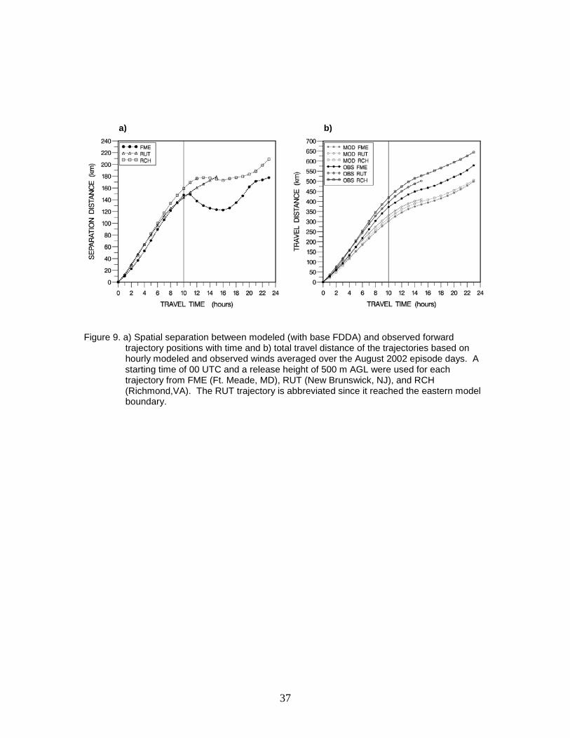
The impact of the modeled and observed wind differences on horizontal transport of

pollutants was further explored using HYSPLIT trajectory analysis. Hourly mean wind

profiles were computed with the model results and observations at selected sites from

the multi-day August episode. The hourly mean modeled and observed wind profiles

were used in the same manner applied by Gilliam et al. (2006) as the time-varying, 3-D

wind fields. In our analysis, a trajectory release height of 500 m AGL was prescribed

with a release time of 00 UTC (2000 local time). The separation distance between the

modeled and observed trajectory positions was computed as well as the total downwind

distance traveled by the modeled and observed trajectories. Figure 9a reveals a steadily

growing spatial separation between the modeled and observed trajectory positions that

reached about 150 km after 10 hours of nighttime travel from each site in the mid-

Atlantic region. Most of the displacement is attributed to the wind speed differences,

however, the modeled wind direction bias also contributed to the growing separation

distance during the night. Thus, the variation in the modeled and observed trajectory

paths indicates that large spatial displacements developed overnight between modeled

and observed pollutant fields aloft. During the daytime hours (i.e., after 12 hours), the

separation distance does not change appreciably indicating better agreement between

the daytime modeled and observed winds. The notable results in Figure 9b show that

observed travel distances are indeed greater than modeled results by about 100 km or

more after 10 hours due primarily to the slower modeled nocturnal wind speeds and

these differences in travel distance prevailed during the duration of the 24-h period.

19

These results reveal that modeled horizontal transport was indeed underestimated along

the mid-Atlantic region during nocturnal periods with strong nocturnal jets. Evidence of

spatial ozone displacements by the model are exhibited in Supplemental Material

(Figures A4, A5).

Sensitivity runs with the WRF model were undertaken using different FDDA options

as well as additional upper air data sets to assess the effects on wind fields and the

nocturnal LLJ during the key August 11-14 episode. Table A1 in Supplemental Material

documents the peak speeds and related characteristics of the nocturnal LLJ indicating

the underestimation by the modeled base case results. From a particular sensitivity run,

Figure 10a,b illustrate the modeled wind flow patterns at ≈ 400 m AGL (layer 7) on

August 11 at 0800 UTC for the base case with FDDA and no FDDA below 2 km

simulations, respectively. A nocturnal jet with higher wind speeds is apparent in the mid-

Atlantic region with a south-southwesterly flow, however, the results in Figure 10b with

no FDDA below 2 km (i.e. below layer 17) exhibit stronger wind speeds in the mid-

Atlantic jet as well as in other areas of the model domain. These dramatic wind field

differences between the base and no FDDA below 2 km cases demonstrates the

negative effect of applying FDDA in the lowest layers (i.e. when PBL heights at night are

<100 m) using the rather coarse vertical resolution of the 3-D OA fields, which could not

adequately resolve the nocturnal LLJ. Clearly, the dynamically-generated fields of the

numerical model were inhibited from fully developing a nocturnal jet in the mid-Atlantic

region since the base FDDA procedure applied weighting to all layers above the shallow

nocturnal PBL height.

The modeled wind speed profiles in Figure 11, averaged over the nocturnal period

from selected sensitivity runs, reveal that increasingly better agreement with the

observed profile occurred as the FDDA weighting coefficient was reduced. The

sensitivity run denoted by profile-assim (SENS9), which involved modification of the

20

original OA fields by the inclusion of all wind profiler data and VAD (Velocity Azimuth

Display) Doppler radar wind measurements (Michelson and Seaman, 2000) along with

no surface FDDA, generated modeled results that were closest to observed winds aloft.

However, the observed average LLJ speed was slightly overestimated and the modeled

LLJ height was slightly lower than the observed jet height. Additional results in Figures

A6, A7 of Supplemental Material show how well the winds aloft are captured over the

diurnal period from various sensitivity runs.

CMAQ was applied with the meteorological fields from the SENS9 run to examine the

impact on maximum ozone fields and maximum 8-h O3 levels relative to the base case

for the August episode. Results for maximum 8-h O3 revealed a mean bias of -10.1 and

-14.5 ppb, and mean error of 12.7 and 16.3 ppb from the base case and SENS9 runs,

respectively, from 397 AQS rural sites. While the SENS9 results contained improved

wind flow fields, horizontal transport was greater which also caused maximum 8-h O3

levels to be slightly lower than in the base case as evident in the mean bias values.

Maximum 8-h O3 levels from the SENS9 results also exhibited underestimates just as in

the base case (Figure 12a). However, Figure 12b reveals that notable differences in

maximum O3 also existed between these simulation results in various areas due to the

horizontal transport differences. In particular, an interesting outcome is demonstrated in

Figure 13 by the O3 concentrations along trajectories originating from the same urban

source locations and for the same release time (11 UTC). Although similar O3

concentrations were generated by both simulations, the trajectories based on these two

different wind fields followed different paths, as anticipated, that impact different

locations downwind after 2 travel days. The stronger and more westerly component in

the SENS9 wind flows caused trajectory paths that were longer and generally to the right

of those in the base case. On the other hand, a trajectory emanating from a Maryland

location in Figure 13b with the stronger nocturnal SENS9 winds reached southern CT,

21

while the base case counterpart in Figure 13a only crossed southern Long Island.

Unfortunately, evaluation results with surface observational site values in CT were

inconclusive regarding which model run provided better performance.

5. Summary

A diagnostic evaluation effort has examined OPE, an indicator of O3 production and

the horizontal transport process in the CMAQ modeling system to take advantage of field

study measurements aloft under primarily high O3 conditions during summer 2002.

Although modeled surface 10 AM O3 and morning residual layer O3 concentrations were

generally found to be biased low at the higher observed concentration levels, modeled

net OPE values were quite comparable to observed results in the mid-afternoon PBL.

Evaluation of modeled base case wind profiles against an independent set of wind

profiler measurements revealed that nocturnal wind speeds were underestimated in the

low level jet and residual layer, and modeled wind directions exhibited a slight southerly

bias in the mid-Atlantic region. Variations in trajectory paths due to observed and

modeled wind flow differences help explain the reason that large spatial displacements

of pollutant patterns can grow over the course of the nocturnal period. Sensitivity

simulations with the WRF meteorological model showed improvements in capturing

nocturnal transport aloft when additional available wind profile data were incorporated

into the FDDA approach and surface nudging was omitted. These results demonstrate

the importance of accurately simulating flow fields aloft, particularly at night, since

overnight transport of O3 and its precursors trapped aloft in the nighttime residual layer

are subsequently entrained to the surface in downwind areas far from emission sources.

While a CMAQ simulation utilizing improved wind fields underestimated maximum O3

levels just as in the base case, a better FDDA approach utilizing more available upper

air data sets was identified to more accurately replicate pollutant transport, which allows

22

a forthcoming diagnostic evaluation to focus on other key input factors and model

processes.

Acknowledgements

Thanks are extended to Stephen Springston (Brookhaven National Laboratory) and

to Russell Dickerson (University of Maryland) for making available their aircraft data

sets. NOAA / ESRL / GSD is recognized for maintenance and access to the MADIS

archive of CAP wind profiler measurements. The VAD data are from the Research Data

Archive (RDA) is maintained by the Computational and Information Systems Laboratory

(CISL) at the National Center for Atmospheric Research (NCAR). NCAR is sponsored

by the National Science Foundation (NSF). The original data are available from the RDA

(http://dss.ucar.edu) in dataset number ds337.0. The U.S. Environmental Protection

Agency through its Office of Research and Development funded and a managed the

research described herein. Although it has been subjected to Agency review and

approved for publication.

References Appel, K.W., Gilliland, A.B., Sarwar, G., Gilliam, R.C., 2007. Evaluation of the

Community Multiscale Air Quality (CMAQ) model version 4.5: Sensitivities impacting

model performance; part I – ozone. Atmospheric Environment, 41, 9603-9615.

Appel, K.W., Roselle, S.J., Gilliam, R.C., Pleim, J.E., 2010. Sensitivity of the Community

Multiscale Air Quality (CMAQ) Model v4.7 results for the eastern United States to

MM5 and WRF meteorological drivers. Geoscientific Model Development, 3, 169-188.

Arnold, J.R., Dennis, R.L., Tonnesen, G.S., 2003. Diagnostic evaluation of numerical air

quality models with specialized ambient observations: testing the Community

Multiscale Air Quality modeling system (CMAQ) at selected SOS 95 ground sites.

23

Atmospheric Environment, 37, 1185-1198, doi:10.1016/S1352-2310(02)01008-7

Byun, D., Schere, K.L., 2006. Review of the governing equations, computational

algorithms, and other components of the Models-3 Community Multiscale Air Quality

(CMAQ) modeling system. Applied Mechanics Reviews, 59, 51-77.

Dennis, R.L., Fox, T., Fuentes, Gilliland, A., Hanna, S., Hogrefe, C., Irwin, J., Rao,

S.T., Scheffe, R., Schere, K., Steyn, D., Venkatram, A., 2010. A framework for

evaluating regional-scale numerical photochemical modeling systems.

Environmental Fluid Mechanics, doi10.1007/s10652-009-9163-2

Gilliam, R.C., Pleim, J.E., 2010. Performance assessment of new land surface and

planetary boundary layer physics in the WRF ARW. Journal of Applied Meteorology

and Climatology,49, 760-774.

Gilliam, R.C., Hogrefe, C., Rao, S.T., 2006. New methods for evaluating meteorological

Models used in air quality applications. Atmospheric Environment, 40, 5073-5086,

doi:10.1016/j.atmosenv.2006.01.023.

Gilliland, A.B., Hogrefe, C., Pinder, R.W., Godowitch, J.M., Foley K.L., Rao, S.T., 2008.

Dynamic evaluations of regional air quality models: Assessing changes in O3

stemming from changes in emissions and meteorology. Atmospheric Environment,

42, 5110-5123.

Godowitch, J.M., Gilliland, A.B., Draxler, R.R., Rao, S.T., 2008a. Modeling assessment

of point source NOX emission reductions on ozone air quality in the eastern United

States. Atmospheric Environment, 42, 87-100.

Godowitch, J.M., Hogrefe,C., Rao, S.T., 2008b. Diagnostic analyses of a regional air

quality model: Changes in modeled processes affecting ozone and chemical-

transport indicators from NOX point source emission reductions. Journal of

Geophysical Research, doi:10.1029/2007JD009537.

Godowitch, J.M., Pouliot, G.A., Rao, S.T., 2010. Assessing multi-year changes in

24

modeled and observed urban NOX concentrations from a dynamic model evaluation

perspective. Atmospheric Environment, 44, 2894-2901, doi:10.1016/

j.atmosenv.2010.04.040

Griffin, R.J., Johnson, C.A., Talbot, R.W., Mao, H., Russo, R.S., Zhou, Y., Sive, B.C.,

2004. Quantification of ozone formation metrics at Thompson Farm during the New

England Air Quality Study (NEAQS) 2002. Journal of Geophysical Research,109,

D24302, doi:10.1029/2004JD005344

Hains, J.C., Taubman, B.F, Thompson, A.M., Stehr, J.W., Marufu, L/.T., Doddridge,

B.G., Dickerson, R.R., 2008. Origins of chemical pollution derived from mid-Atlantic

aircraft profiles using a clustering technique. Atmospheric Environment, 42, 1727-

1741, doi:10.1016/j.atmosenv.2007.11.052

Hegarty, J., Mao, H., Talbot., 2007. Synoptic controls on summertime surface ozone in

the northeastern United States. Journal of Geophysical Research, 112, D14306,

doi:10.1029/2006JD008170

Hogrefe, C., Biswas, J., Lynn, B., Civerolo, K., Ku, J,Y., Rosenthal, J., Rosenweig, C.,

Goldberg, R., Kinney, P.L., 2004. Simulating regional-scale ozone climatology over

the eastern United States: model evaluation results. Atmospheric Environment, 38,

2627-2638, doi:10.1016/j.atmosenv.2004.02.033

Kleinman, L.I., Daum, P.H., Lee, Y.N., Senum, G.I., Springston, S.R., Wany, J.,

Berkowitz, C., Hubbe, J., Zaveri, R.A., Brechtel, F.J., Jayne, J., Onasch, T.B.,

Worsnop, D., 2007. Aircraft observations of aerosol composition and ageing in New

England and mid-Atlantic states during the summer 2002 New England Air Quality

Study field campaign. Journal of Geophysical Research, 112, D09310,

doi:10.1029/2006JD007786

Lin, C. ,2008. Impact of downward mixing ozone on surface ozone accumulation in

southern Taiwan. Journal of Air and Waste Management Association, 58:562-579,

25

doi:10.3155/1047-3289.58.4.562

Luecken, D.J., Phillips, S., Sarwar, G., Jang, C., 2008. Effects of using the CB05 vs

SAPRC99 vs CB4 chemical mechanism on model predictions: Ozone and gas-phase

photochemical precursor concentrations. Atmospheric Environment, 42, 5805-5820,

doi:10.1016/j.atmosenv.2007.08.056

Mao, H., Chen, M., Hegarty, J.D., Talbot, R.W., Koermer, J.P., Thompson, A.M., Avery,

M.A., 2010. A comprehensive evaluation of seasonal simulations of ozone in the

northeastern US during summers 2001-2005. Atmospheric Chemistry and Physics,

10, 9-27.

Michelson, S.A., and Seaman, N. L., 2000. Assimilation of NEXRAD-VAD winds in

summertime meteorological simulations over the northeastern United States. J. Appl.

Meteor., 39, 367-383.

Olszyna, K.F., Bailey, E.M., Simonaitis, R., Meagher, J.F., 1998. O3 and NOY

relationships at a rural site. Journal of Geophysical Research, 77, D7, 14557-14563,

doi:10.1029/94JD00739

Otte, T., 2008: The impact of nudging in the meteorological model for retrospective air

quality simulations. Part I: Evaluation against National Observation Networks. Journal

of Applied Meteorology and Climatology, 47, 1853-1867, doi:10.1175/2007

JAMC1790.1

Pierce, T., Hogrefe, C., Rao, S.T., Porter, P.S., Ku, J., 2010. Dynamic evaluation of a

regional air quality model: Assessing the emissions-induced weekly ozone cycle,

Atmospheric Environment, 44, 3583-3596, doi: 10.1016/j.atmosenv.2010.05.046

Ryan, W.F, Doddridge, Dickerson, R.R., Morales, R.M., Hallock, K.A., Roberts, P.T.,

Blumenthal, D.L., Anderson, J.A., Civerolo, K.L., 1998. Pollutant transport during a

regional O3 episode in the mid-Atlantic states. Journal of Air and Waste Management

Association, 48:786-797.

26

Springston, SR., Kleinman, L.I., Brechtel, F., Lee, Y.-N., Nunnermacker, L.J., Wang, J.,

2005. Chemical evolution of an isolated power plant plume during the TexAQS 2000

study, Atmospheric Environment, 39, 3431-3443.

Stauffer, D.R., Seaman, N.L., Binkowski, F.S., 1991: Use of four-dimensional data

assimilation in a limited area mesoscale model. Part II: Effects of data assimilation

within the planetary boundary layer. Monthly Weather Review, 119, 734-754.

Taubman, B.F., Hains, J.C., Thompson, A.M., Marufu, L.T., Doddridge, B.G., Stehr,

J.W., Piety, C.A., Dickerson, R.R., 2006. Aircarft vertical profiles of trace gas and

aerosol pollution over the mid-Atlantic United States: Statistics and meteorological

cluster analysis. Journal of Geophysical Research, 111, D10S07,

doi:10.1029/2005JD006196

Taubman, B.F., Marufu, L.T., Piety, C.A., Doddridge, B.G., Stehr, J.W., Dickerson, R.R.,

2004. Airborne characterization of the chemical, optical and meteorological properties

and origins of a combined ozone-haze episode in the eastern United States. Journal

of Atmospheric Sciences, 61, 1781-1793.

Vukovich, F.M., Scarborough, J., 2005. Aspects of ozone transport, mixing, and

chemistry in the greater Maryland area. Atmospheric Environment, 39, 7008-7019,

doi:10.1016/j/atmosenv.2005.07.054

Yu, S., Mathur, R., Kang, D., Schere, K., Eder B., Pleim, J., 2006. Performance and

diagnostic evaluation of ozone predictions by the Eta-Community Multiscale Air

Quality forecast system during the 2002 New England Air Quality Study. Journal of

Air and Waste Management Association, 56:1459-1471.

Zhang, D., Zhang, S., Weaver, S.J., 2006. Low-level jets over the mid-Atlantic states:

Warm season climatology and a case study. Journal of Applied Meteorology and

Climatology, 45, 194-209.

Zhang, J., Rao, S.T., 1999. The role of vertical mixing in the temporal evolution of

27

ground-level ozone concentrations. Journal of Applied Meteorology, 38, 1674-1691.

Zhang, K., Mao, H., Civerolo, K., Berman, S., Ku, J.Y., Rao, S.T., Doddridge, B.,

Philbrick, C.R., Clark, R., 2001. Numerical investigation of boundary layer evolution

and nocturnal low-level jets: local versus non-local PBL schemes. Environmental

Fluid

Mechanics, 1, 171-208.

List of Figures Figure 1. Modeled and observed mean and 95th percentile values of daily maximum 8-hour ozone concentrations determined from results at rural CASTNET site locations in the eastern US during the 92 day period from June 1 through August 31, 2002. Figure 2. a) Modeled and observed UM aircraft ozone profiles at S. Albany, NY near 17 UTC on August 12, 2002, b) paths of backtrajectories released at 500 m and 1000 m AGL at the same time as the profiles in a) and traveling 80 hours backward in time, c) modeled hourly ozone concentrations at backtrajectory positions at 500 m and below in layer 1. Vertical dashed lines in c) designate the time of sunrise on each day of this travel period. Figure 3. a) Modeled ozone concentrations at 10 AM (local time) versus observed 10 AM ozone levels from rural eastern surface AQS sites during summer 2002 ozone episode days and b) modeled residual layer ozone versus observed residual layer ozone levels from UM aircraft profiles obtained during summer 2002 experimental days. The box/whisker results depict values at the median (line inside the boxes), box edges denote the 25th

and 75th percentiles and whiskers extend to the 10th and 90th percentiles. Figure 4. Mid-morning average modeled and observed UM aircraft ozone profiles a) from all sites in the mid-Atlantic region during June/July 2002 experimental cases and b) from 3 sites in VT/NH during August 13, 2002. The dashed lines represent ± 1 standard deviation (SD) from the average values. Figure 5. Modeled and UM aircraft average ozone profiles from mid-Atlantic and New England locations from mid-afternoon periods during summer 2002 episode cases. Height (z) is

28

normalized by the PBL height (Zi). Dashed lines represent concentrations at ± 1 standard deviation (SD) from average values. Figure 6. Relationship between ozone and NOZ from model results and BNL aircraft measurements along horizontal traverses near the middle of the PBL in the mid- afternoon during summer 2002 field study days. Lines depict the slopes from linear regression fits to the modeled and observed results. Each symbol represents a value derived over 5% increments of the observed and modeled concentration distributions. Figure 7. Vertical time section of the average wind speed difference (modeled – observed) over the diurnal cycle based on modeled and observed profiles from all eastern radar wind profiler sites during the summer 2002 period. Isopleths are given in units of m/s. Figure 8. Modeled (gray) and observed (rose) a) wind speed and b) direction profiles averaged over the nocturnal periods of August 11-15, 2002 at Ft. Meade, MD. Boxes span the 25th to 75th percentiles, and whiskers in a) extend from 10th to 90th percentiles. Figure 9. a) Spatial separation between modeled (with base FDDA) and observed forward trajectory positions with time and b) total travel distance of the trajectories based on hourly modeled and observed winds averaged over the August 2002 episode days. A starting time of 00 UTC and a release height of 500 m AGL were used for each trajectory from FME (Ft. Meade, MD), RUT (New Brunswick, NJ), and RCH (Richmond, VA). The RUT trajectory is abbreviated because it reached the eastern model boundary. Figure 10. Wind flows depicting speeds (color tiles) and directions (arrows) near 500 m AGL at 0800 UTC on August 11, 2002 from WRF simulations. a) base FDDA and b) no FDDA below 2 km AGL. . Figure 11. Modeled results averaged over the nocturnal period from different WRF simulations using different FDDA options versus an observed nocturnal average wind speed profile at Ft. Meade, MD from August 11, 2002. The observed profile has been truncated near 1000 m since profile data above this level were not available during all hours. Figure 12. a) Modeled maximum 8-h O3 field using improved wind fields (SENS9) on August 12, 2002 and AQS site values (circles, and b) differences in maximum 8-h O3 (SENS9 – base) results. Figure 13. Ozone from CMAQ runs is depicted along the paths of forward trajectories released at 500 m AGL on August 11, 2002 starting at 1100 UTC and traveling 50 hours downwind of selected locations using a) base case and b) SENS9 sensitivity run wind fields.

29

Figure 1. Modeled and observed mean and 95th percentile values of daily maximum 8-hour ozone concentrations determined from results at rural CASTNET site locations in the eastern US over the 92 day period from June 1 through August 31, 2002.

30

Figure 2. a) Modeled and observed UM aircraft ozone profiles near S. Albany, NY at 17 UTC on August 12, 2002, b) paths of backward trajectories released at 500 m and 1000 m AGL at the same time as the profiles in a) and traveling 80 hours backward in time, c) modeled hourly ozone concentrations at backward trajectory positions at 500 m and below in layer 1. Vertical dashed lines in c) designate the time of sunrise on each day of this travel period.

a) b) c)

31

Figure 3. a) Modeled ozone concentrations at 10 AM versus observed 10 AM ozone levels from rural eastern surface AQS sites during summer 2002 ozone episode days and b) modeled residual layer ozone versus observed residual layer ozone levels from UM aircraft profiles obtained during summer 2002 experimental days. The box/whisker results depict values at the median (line inside the boxes), box edges denote the 25th and 75th percentiles and whiskers extend to the 10th and 90th percentiles.

32

a) b)

Figure 4. Mid-morning average modeled and observed UM aircraft ozone profiles a) from all sites in the mid-Atlantic region during June/July 2002 experimental cases and b) from 3 sites in VT/NH during August 13, 2002. The dashed lines represent ± 1 standard deviation (SD) from the average values.

33

Figure 5. Modeled and UM aircraft average ozone profiles from mid-Atlantic and New England locations from mid-afternoon periods during summer 2002 episode cases. Height (z) is normalized by the PBL height (zi). The dashed lines represent concentrations at ± 1 standard deviation (SD) from the average values.

34

Figure 6. Relationship between ozone and NOZ from model results and BNL aircraft measurements along horizontal traverses near the middle of the PBL in the mid- afternoon during summer 2002 field study days. Lines depict linear regression fit to the modeled and observed results for NOZ values ≤ 8 ppb. Each symbol is derived from groups of values over 5% intervals of the observed and modeled concentration distributions.

35

Figure 7. Vertical time section of the average wind speed difference (modeled – observed) over the diurnal cycle based on modeled and observed profiles from all eastern radar wind profiler sites during the summer 2002 period. Isopleths are given in units of m/s.

36

Figure 8. Modeled (gray) and observed (rose) a) wind speed and b) direction profiles averaged over the nocturnal periods of August 11-15, 2002 at Ft. Meade, MD. Boxes span the 25th to 75th percentiles, and whiskers in a) extend from 10th to 90th percentiles.

a) b)

37

Figure 9. a) Spatial separation between modeled (with base FDDA) and observed forward trajectory positions with time and b) total travel distance of the trajectories based on hourly modeled and observed winds averaged over the August 2002 episode days. A starting time of 00 UTC and a release height of 500 m AGL were used for each trajectory from FME (Ft. Meade, MD), RUT (New Brunswick, NJ), and RCH (Richmond,VA). The RUT trajectory is abbreviated since it reached the eastern model boundary.

a) b)

38

a)

b)

Figure 10. Wind flows depicting speeds (color tiles) and directions (arrows) near 500 m AGL at 0800 UTC on August 11, 2002 from WRF simulations with a) base FDDA and b) no FDDA below 2 km AGL.

39

Figure 11. Modeled results averaged over the nocturnal period from different WRF simulations using different FDDA options versus an observed nocturnal average wind speed profile at Ft. Meade, MD from August 11, 2002. The observed profile has been truncated near 1000 m since profile data above this level were not available during all hours.

40

a)

b)

Figure 12. a) Modeled maximum 8-h O3 field using improved wind fields (SENS9) on August 12, 2002 and AQS site values (circles), and b) differences in maximum 8-h O3 (SENS9 - base) results.

41

a)

b)

Figure 13. Ozone from CMAQ runs is depicted along the paths of forward trajectories released at 500 m AGL on August 11, 2002 starting at 1100 UTC and traveling for 50 hours downwind of select locations using a) base case and b) SENS9 sensitivity run wind fields.

42

a) b)

Figure A1. Wind speed fields on August 11, 2002 at 0700 UTC in layer 5 ( ≈300 m AG L) from FDDA base case simulations with the a) MM5 and b) WRF meteorological models.

43

Figure A2. Hourly rate of change in ozone concentration at rural and urban AQS sites (black) and paired modeled results (gray) from episode days during summer 2002. The vertical line denotes 10 AM local time when the nocturnal inversion layer is often completely eroded and chemical production of ozone begins to be a greater contributor to increasing the ozone concentration.

44

Table A1. Observed Nocturnal Jet Peak Speed and Associated Characteristics versus Model Results at Ft. Meade, MD from the August 2002 episode days Profiler Observations Model* Results ___________________ ___________________ Peak Day JD Hr Z WS WD Z WS WD (UTC) (m AGL) (m/s) (deg) (m AGL) (m/s) (deg) 11 223 08 454. 15.3 225. 386. 11.7 211. 12 224 06 454. 14.9 232. 268. 10.2 205. 13 225 05 344. 9.7 224. 193. 7.6 197. 14 226 06 729. 16.9 234. 386. 9.6 198. 15 227 05 783. 18.3 228. 386. 13.9 201. ______________________________________________________ * Results from MM5 base simulation with FDDA used in the CMAQ simulations

45

Figure A3. Model (base case) wind speed on August 11, 2002 at 300 m (layer 5) at 08 UTC and observed wind speeds at the same height from profiler sites.

46

Figure A4. CMAQ ozone field and observed ozone along the BNL aircraft horizontal traverse in The northeastern US at 1900 UTC on July 21, 2002. Underestimated model winds caused the high ozone pattern in western PA to be several hours slow in arriving in the area of the flight path in elevated ozone along the NY/PA border, while the modeled high ozone area in the NY Hudson Valley/ western CT should be situated in central CT indicating modeled speeds were biased low.

47

Figure A5. Another example of spatial displacement of the modeled ozone pattern versus observed ozone from vertical profiles of the UM aircraft in the Richmond, VA area in the mid-morning of June 11, 2002. Comparisons of modeled and observed wind profiles from the nocturnal period indicated the modeled wind speeds at this level (layer 7 ~ 400 m AGL) underestimated observed winds causing the high ozone area along the VA/NC border to be slow in arriving in the Richmond, VA area where the profiles were made.

48

Selected FDDA sensitivity runs with the WRF model are defined below with the results shown in the following supplemental figures. Sensitivity Case Definition List Base: surface nudging and 3-D OA nudging of winds above PBL SENS3: no surface nudging or 3-D nudging below 2000 m SENS5: no surface nudging and no u,v nudging in PBL SENS6: no surface nudging and no u,v nudge in PBL + 500 m SENS7: no surface nudging, spectral nudging with 250 km filter applied SENS8: profiler data assimilated, with no surface nudging and no 3-D PBL nudging SENS9: all wind profiles included (profiler sites, VAD radar profiles, and rawinsondes) SENS10: SENS5, except with 47 layers SENS11: lowest nudging level set at 1000 m, except when PBL height is greater, then lowest nudging level is set to PBL + 1 level.

49

Figure A6. Modeled wind speed results from WRF simulations using different FDDA optional procedures compared to observed wind speeds from 4 mid-Atlantic profiler sites at 450 m AGL (bottom) and 1000 m AGL (top).

1000 m Diurnal Wind Speed (m/s)

0

1

2

3

4

5

6

7

8

0 3 6 9 12 15 18 21

Hour (UTC)

Win

d Sp

eed

(m/s

)

PROFILERSBASESENS3SENS5SENS6SENS7SENS8SENS9SENS10

450 m Diurnal Wind Speed (m/s)

0

2

4

6

8

10

12

14

0 3 6 9 12 15 18 21

Hour (UTC)

Win

d Sp

eed

(m/s

)

PROFILERSBASESENS3SENS5SENS6SENS7SENS8SENS9SENS10SENS11

50

Figure A7. Modeled wind direction results from WRF simulations using different FDDA optional procedures compared to observed directions from 4 mid-Atlantic wind profiler sites at 450 m AGL (bottom) and 1000 m AGL (top).

1000 m Diurnal Wind Direction

150

180

210

240

270

0 3 6 9 12 15 18 21

Hour (UTC)

Win

d D

irect

ion

(deg

)

PROFILERSBASESENS3SENS5SENS6SENS7SENS8SENS9SENS10

450 m Diurnal Wind Direction

150

180

210

240

270

0 3 6 9 12 15 18 21

Hour (UTC)

Win

d D

irect

ion

(deg

)

PROFILERSBASESENS3SENS5SENS6SENS7SENS8SENS9SENS10

51