Diffusion coefficients and radial distribution functions of NaCl and

HMT-PMBI(Cl−) determined using molecular dynamics

simulations with periodic boundary conditions

Colton Lohn

Department of Physics, Simon Fraser University, Burnaby BC Canada

Abstract

The relationship between system size and diffusivity in a periodic cubic simulation cell was studied.

The diffusion coefficients of Na+ and Cl− in TIP4P/2005 water show significant system-size dependence.

No such system-size effects were found for either the diffusion coefficient of Cl− or the radial distribu-

tion functions for chloride–oxygen, chloride–chloride, chloride–nitrogen, and chloride–carbon in 87.5%

methylated HMT-PMBI at hydration level λ = 16 using TIP4P/2005 water.

Introduction

Molecular dynamics simulations have emerged as an indispensable tool for studying the nanoscopic, meso-

scopic, and macroscopic properties of matter. These simulations frequently make use of a periodic boundary

simulation cell. In a periodic cell, particles can pass through the cell boundary and re-emerge on the opposite

side. This allows a finite system to act as if it is infinite, and therefore bulk properties can be investigated

without the use of large computationally demanding systems. However, in a periodic system, it is possible

for a particle to interact with itself through the periodic boundary. This becomes particularly problematic

with long-range interactions, such as the Coulombic r−1 interaction, as well as hydrodynamic interactions

which also exhibit r−1 decay.1 This self-interaction introduces a system-size dependence which can result in

the underestimation of diffusivity.2

We first perform molecular dynamics simulations of NaCl aqueous solution using various water models.

Diffusion coefficients and radial distribution functions are subsequently calculated. We then compare our

results to those from Cheatham3 and from experiment. Next, we investigate the relationship between system

size and diffusivity. Finally, we look at whether this relationship exist in systems of poly-(hexamethyl-p-

terphenylbenzimidazolium), referred to as HMT-PMBI.

1

Methods

Molecular dynamics simulations were performed in LAMMPS,4 an open source classical molecular dynamics

code. The OPLS force field was used to model interatomic interactions. The functional form of this force

field consists of harmonic bond stretching and angle bending terms, a Fourier series for dihedral energetics,

and Coulomb and Lennard-Jones terms for nonbonded interactions.

Ebonds = kr,i(ri − r0,i)2, (1)

Eangles = kθ,i(θi − θ0,i)2, (2)

Edihedrals =V1,i2

(1 + cos(φi)) +V2,i2

(1− cos(2φi))+

V3,i2

(1 + cos(3φi)) +V4,i2

(1− cos(4φi)),

(3)

Enonbonded =qiqje

2

4πε0rij+ 4εij

[(σijrij

)12

−(σijrij

)6]. (4)

Here, kr,i and kθ,i are force constants, V1,i, V2,i, V3,i, and V4,i are Fourier coefficients, qi and qj are the partial

atomic charges, εij is the well depth for the Lennard-Jones potential, and σij is the finite distance where

the Lennard-Jones potential is zero. The parameters εij and σij were obtained using geometric combination

rules εij = (εiεj)1/2 and σij = (σiσj)

1/2.

NaCl

The diffusion coefficients and radial distribution functions of Na+ and Cl− were investigated using the three-

site water model, SPC/E,5 and the four-site water models, TIP4P-Ew6 and TIP4P/2005.7 Three-site water

models describe three points of interaction, each assigned a charge and Lennard-Jones parameters. It is,

however, common to treat hydrogen as a point particle with no Lennard-Jones potential. Four-site water

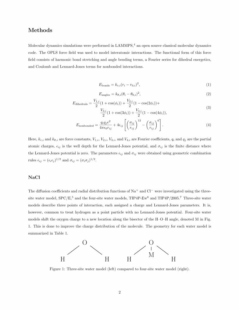
models shift the oxygen charge to a new location along the bisector of the H–O–H angle, denoted M in Fig.

1. This is done to improve the charge distribution of the molecule. The geometry for each water model is

summarized in Table 1.

���

ZZZ

O

H H

���

ZZZ

O

MH H

Figure 1: Three-site water model (left) compared to four-site water model (right).

2

SPC/E5 TIP4P-Ew6 TIP4P/20057

O–H distance (A) 1.0 0.9572 0.9572

H–O–H angle 109.47◦ 104.52◦ 104.52◦

O–M distance (A) 0.1250 0.1546

Table 1: Water molecule geometries.

All of these water models are rigid, meaning the O–H distance and H–O–H angle are fixed. Therefore,

all interactions are described by the nonbonded term of the OPLS force field (Eq. 4). The water model

parameters were previously determined to imitate the various properties of water,5–7 while the ion parameters

were optimized to reproduce their experimental hydration free energies and other quantities.8,9 Both water

and ion parameters are summarized in Table 2.

SPC/E5,8 TIP4P-Ew6,8 TIP4P/20057,9

qi

(e)

εi

(kcal/mol)

σi

(A)

qi

(e)

εi

(kcal/mol)

σi

(A)

qi

(e)

εi

(kcal/mol)

σi

(A)

O −0.8476 0.1553 3.166 −1.0484 0.1628 3.1644 −1.1128 0.1852 3.1589

H 0.4238 0 0 0.5242 0 0 0.5564 0 0

Na+ 1 0.3526 2.160 1 0.1684 2.185 1 0.0005 4.07

Cl− −1 0.0128 4.831 −1 0.0117 4.918 −1 0.71 4.02

Table 2: Charges and Lennard-Jones parameters for water and ions.

The simulation cells were initialized using the PACKMOL software package.10 This package returns

the coordinates for the desired atoms and molecules which have been randomly distributed within the cell,

separated by at least the specified distance tolerance. Each of the simulation cells consisted of a cubic periodic

box of side length 40 A containing 1500 water molecules and 27 ion pairs. This gives a concentration of

approximately 1 mol/kg.

In LAMMPS, the direct nonbonded interaction cutoff was set to 9 A. This means that the nonbonded

energy between water molecules and ions was only evaluated when they were separated by distances less than

the cutoff. At distances greater than the cutoff, electrostatic interactions were calculated using the particle-

particle particle-mesh solver with accuracy 5 × 10−4. The SHAKE algorithm11 was used to constrain the

water molecule geometries with a tolerance of 10−5 A. A simulation timestep of 2 fs was used. The target

temperature was set to 298 K, while the target pressure was set to 0.9869 atm. Temperature and pressure

time constants were 200 fs and 2000 fs, respectively. The system energies were minimized using the conjugate

gradient method for 1000 iterations. The systems were subsequently equilibrated at constant volume (NVT)

for 40 ps and then at constant pressure (NPT) for another 40 ps. Finally, simulations were performed at

3

constant volume (NVT) for 10 ns. A snapshot of the simulation cell is shown in Fig. 2a. A performance of

approximately 39 ns/day was acheived with 16 CPU cores on the Cedar cluster at Simon Fraser University.

For a 3 dimensional system, the diffusion coefficient is related to the mean squared displacement by,

D = limt→∞

∂

∂t

〈|r(t)− r0|2〉6

. (5)

Therefore, the diffusion coefficient can be determined using least squares fitting to estimate the slope of

the mean squared displacement over time. For a single particle, very long simulation times are required to

obtain accurate results; however, averaging over an ensemble of identical particles significantly improves the

statistics allowing for shorter run times.12

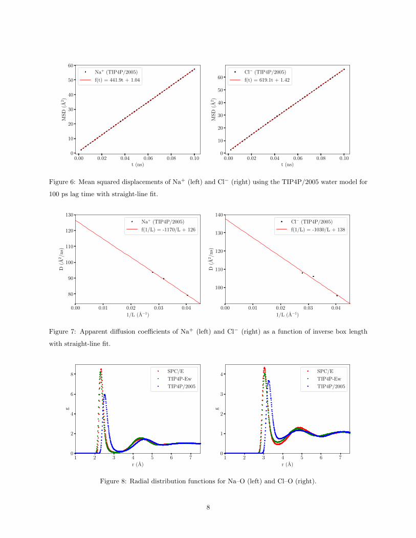
The systems were analyzed using VMD,13 a visualization program for large molecular systems. The

diffusion coefficient tool14 was used to calculate the mean squared displacements of Na+ and Cl− for a 100

ps lag time with a 1 ps timestep, shown in Fig. 3. The associated instantaneous diffusion coefficients are

displayed in Fig. 4. To reproduce the methods used by Cheatham,3 a straight-line fixed at the origin was

fit by least squares to the plots of mean squared displacement for a 10 ps lag time. The fits for TIP4P/2005

are shown in Fig. 5. The diffusion coefficients were subsequently calculated and the results are summarized

in Table 3.

This Research Cheatham3

SPC/E TIP4P-Ew TIP4P/2005 SPC/E TIP4P-Ew Exp.15

Volume (103 A3) 45.32 44.97 46.34 45.61 45.65

Na+ (A2/ns) 123 ± 4 97 ± 3 121 ± 4 108 ± 18 93 ± 18 133.4

Cl− (A2/ns) 151 ± 4 130 ± 4 142 ± 5 144 ± 20 138 ± 22 203.2

Table 3: Calculated diffusion coefficients for sodium chloride aqueous solution using 10 ps lag time and fixed

origin straight-line fit compared with Cheatham and experimental values for infinite dilution.

We see good agreement with the results from Cheatham; however, using a lag time as short as 10 ps

results in fitting mostly the ballistic regime. This can be seen by a lack of convergence for the instantaneous

diffusion at short times in Fig. 4. To avoid this, a straight-line was fit by least squares to the plots of mean

squared displacement for the entire 100 ps lag time. The fits for TIP4P/2005 are shown in Fig. 6. The

results are summarized in Table 4. As expected, we see lower values for the diffusion coefficients, giving

worse agreement with the experimental results. This discrepancy is partly due to concentration effects.

The experimental diffusion coefficients were determined at infinite dilution, and therefore we expect them

to be higher. This is because the diffusion coefficient is inversely proportional to ion concentration.16 A

dependence on the simulation cell size may also have contributed to this disagreement with experiment. One

way to check for this is to extrapolate to an infinite system size. This can be done by performing a linear fit

4

to the plot of apparent diffusion coefficients with respect to the reciprocal of the cubic simulation cell length.

The corrected value is then given by the vertical intercept.

SPC/E TIP4P-Ew TIP4P/2005 Exp.15

Volume (103 A3) 45.32 44.97 46.34

Na+ (A2/ns) 85.64 ± 0.02 73.65 ± 0.03 93.71 ± 0.05 133.4

Cl− (A2/ns) 109.86 ± 0.09 103.2 ± 0.11 108.0 ± 0.11 203.2

Table 4: Calculated diffusion coefficients for sodium chloride aqueous solution using 100 ps lag time and

straight-line fit compared with experimental values at infinite dilution.

The system-size dependence was investigated using the TIP4P/2005 water model. Two additional sim-

ulations were performed using smaller system sizes. All system configurations are summarized in Table 5.

These systems were simulated using the same methods as previously mentioned. The apparent diffusion

coefficients were measured for Na+ and Cl− for each system size. They were then plotted as a function of

inverse simulation cell length and fit by least squares with a straight-line, shown in Fig. 7. The corrected

diffusion coefficients were extracted and are summarized in Table 6. We see an increase of approximately

35% for Na+ and 28% for Cl− over the previous highest values, indicating a significant dependence on system

size.

System 1 System 2 System 3

Water Molecules 500 1000 1500

Ion Pairs 9 18 27

Volume (103 A3) 15.19 30.97 46.34

Table 5: System configurations used for size correction.

System 1 System 2 System 3 Corrected Exp.15

Na+ (A2/ns) 79.20 ± 0.07 89.61 ± 0.04 93.71 ± 0.05 126 ± 1.6 133.4

Cl− (A2/ns) 95.5 ± 0.11 106.08 ± 0.08 108.0 ± 0.11 138 ± 6 203.2

Table 6: Corrected diffusion coefficients using TIP4P/2005 compared with experimental values at infinite

dilution.

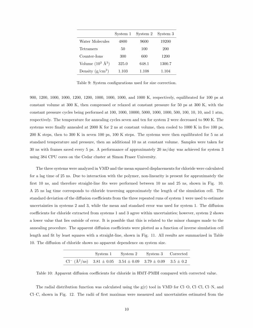
The radial distribution function describes the probability of finding a particle at a distance r from a

reference particle relative to the average particle density of the system. The ion–oxygen radial distribution

functions for Na+ and Cl− with each water model were computed using the g(r) tool in VMD with a

resolution of 0.01 A, as seen in Fig. 8. The first hydration shells are given by the first maximum of the

ion–oxygen radial distribution functions and are summarized in Table 7. The first maxima from the two

5

smaller TIP4P/2005 systems were also calculated and the standard deviation of the three systems was used

as an estimate for uncertainty. We see good agreement with experimental values for Na+ used with SPC/E

and TIP4P-Ew; however, Cl− values are underestimated. Using TIP4P/2005 gives an overestimate for both

Na+ and Cl−. The coordination number is the total number of nearest neighbours to a central atom and was

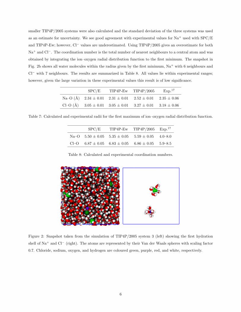
obtained by integrating the ion–oxygen radial distribution function to the first minimum. The snapshot in

Fig. 2b shows all water molecules within the radius given by the first minimum, Na+ with 6 neighbours and

Cl− with 7 neighbours. The results are summarized in Table 8. All values lie within experimental ranges;

however, given the large variation in these experimental values this result is of low significance.

SPC/E TIP4P-Ew TIP4P/2005 Exp.17

Na–O (A) 2.34 ± 0.01 2.31 ± 0.01 2.52 ± 0.01 2.35 ± 0.06

Cl–O (A) 3.05 ± 0.01 3.05 ± 0.01 3.27 ± 0.01 3.18 ± 0.06

Table 7: Calculated and experimental radii for the first maximum of ion–oxygen radial distribution function.

SPC/E TIP4P-Ew TIP4P/2005 Exp.17

Na–O 5.50 ± 0.05 5.35 ± 0.05 5.59 ± 0.05 4.0–8.0

Cl–O 6.87 ± 0.05 6.83 ± 0.05 6.86 ± 0.05 5.9–8.5

Table 8: Calculated and experimental coordination numbers.

Figure 2: Snapshot taken from the simulation of TIP4P/2005 system 3 (left) showing the first hydration

shell of Na+ and Cl− (right). The atoms are represented by their Van der Waals spheres with scaling factor

0.7. Chloride, sodium, oxygen, and hydrogen are coloured green, purple, red, and white, respectively.

6

0.00 0.02 0.04 0.06 0.08 0.10t (ns)

0

10

20

30

40

50

60

MS

D(A

2)

SPC/E

TIP4P-Ew

TIP4P/2005

0.00 0.02 0.04 0.06 0.08 0.10t (ns)

0

10

20

30

40

50

60

70

MS

D(A

2)

SPC/E

TIP4P-Ew

TIP4P/2005

Figure 3: Mean squared displacements of Na+ (left) and Cl− (right) for 100 ps lag time.

0.00 0.02 0.04 0.06 0.08 0.10t (ns)

80

100

120

140

160

180

200

220

D(A

2/n

s)

SPC/E

TIP4P-Ew

TIP4P/2005

0.00 0.02 0.04 0.06 0.08 0.10t (ns)

100

120

140

160

180

200

220

240D

(A2/n

s)SPC/E

TIP4P-Ew

TIP4P/2005

Figure 4: Instantaneous diffusion coefficients of Na+ (left) and Cl− (right) for 100 ps lag time.

0.002 0.004 0.006 0.008 0.010t (ns)

1

2

3

4

5

6

7

MS

D(A

2)

Na+ (TIP4P/2005)

f(t) = 580t

0.002 0.004 0.006 0.008 0.010t (ns)

2

4

6

8

MS

D(A

2)

Cl− (TIP4P/2005)

f(t) = 780t

Figure 5: Mean squared displacements of Na+ (left) and Cl− (right) using the TIP4P/2005 water model for

10 ps lag time with fixed origin straight-line fit.

7

0.00 0.02 0.04 0.06 0.08 0.10t (ns)

0

10

20

30

40

50

60M

SD

(A2)

Na+ (TIP4P/2005)

f(t) = 441.9t + 1.04

0.00 0.02 0.04 0.06 0.08 0.10t (ns)

0

10

20

30

40

50

60

MS

D(A

2)

Cl− (TIP4P/2005)

f(t) = 619.1t + 1.42

Figure 6: Mean squared displacements of Na+ (left) and Cl− (right) using the TIP4P/2005 water model for

100 ps lag time with straight-line fit.

0.00 0.01 0.02 0.03 0.04

1/L (A−1)

80

90

100

110

120

130

D(A

2/n

s)

Na+ (TIP4P/2005)

f(1/L) = -1170/L + 126

0.00 0.01 0.02 0.03 0.04

1/L (A−1)

100

110

120

130

140D

(A2/n

s)

Cl− (TIP4P/2005)

f(1/L) = -1030/L + 138

Figure 7: Apparent diffusion coefficients of Na+ (left) and Cl− (right) as a function of inverse box length

with straight-line fit.

1 2 3 4 5 6 7

r (A)

0

2

4

6

8

g

SPC/E

TIP4P-Ew

TIP4P/2005

1 2 3 4 5 6 7

r (A)

0

1

2

3

4

g

SPC/E

TIP4P-Ew

TIP4P/2005

Figure 8: Radial distribution functions for Na–O (left) and Cl–O (right).

8

HMT-PMBI

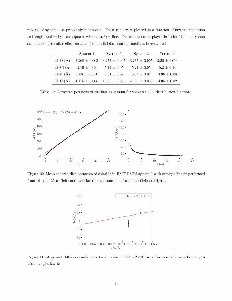
The system-size dependence of diffusion and radial distribution functions of chloride in poly-(hexamethyl-p-

terphenylbenzimidazolium), referred to as HMT-PMBI, were investigated. The systems consisted of HMT-

PMBI tetramers that have 87.5% of their nitrogens functionalized with a methyl group and were at a

hydration level λ = 16. The hydration level gives the number of water molecules per counter-ion. The

hydrated HMT-PMBI chloride system is shown in Fig 9. The TIP4P/2005 water model and associated

chloride parameters were used.7,9 All HMT-PMBI paramters and topologies are consistent with the methods

of Schibli.18 The all-atom parameterization of the OPLS force field (OPLS-AA) was used to describe the

polymer backbones.19 Improper dihedral angles were described using Eimproper = kφ(1 + d cos(nφ)).

Figure 9: Snapshot taken from the simulation of HMT-PMBI system 1 (left) showing Cl− in the pores of the

polymer with water molecules removed (center) and an isolated tetramer (right). The atoms are represented

by their Van der Waals spheres with scaling factor 0.7. Chloride, oxygen, nitrogen, carbon, and hydrogen

are coloured green, red, blue, grey, and white, respectively.

The systems 1–3 described in Table 9 were initialized using PACKMOL in periodic boxes with lengths

120 A, 150 A, and 200 A, respectively. To estimate uncertainties, two additional copies of system 1 were

initialized in PACKMOL using different random seeds. In LAMMPS, the nonbonded interaction cutoff was

set to 8.5 A. The long-range electrostatic interactions were calculated using the particle-particle particle-mesh

solver with accuracy 5× 10−4. The SHAKE algorithm was used to constrain the water molecule geometries

with a tolerance of 10−5 A. Temperature and pressure damping constants were set to 100 fs and 1000 fs,

respectively.

The system energies were minimized using the conjugate gradient method for 106 iterations or until the

stopping tolerance of 10−5 was reached. The systems were then annealed at constant volume at 1200 K for

600 ps to randomize the backbone configurations. They were then subjected to eleven annealing-relaxation-

compression cycles, in which the systems were annealed for 50 ps at constant volume at temperatures 1200,

9

System 1 System 2 System 3

Water Molecules 4800 9600 19200

Tetramers 50 100 200

Counter-Ions 300 600 1200

Volume (103 A3) 325.0 648.1 1300.7

Density (g/cm3) 1.103 1.108 1.104

Table 9: System configurations used for size correction.

900, 1200, 1000, 1000, 1200, 1200, 1000, 1000, 1000, and 1000 K, respectively, equilibrated for 100 ps at

constant volume at 300 K, then compressed or relaxed at constant pressure for 50 ps at 300 K, with the

constant pressure cycles being performed at 100, 1000, 10000, 5000, 1000, 1000, 500, 100, 10, 10, and 1 atm,

respectively. The temperature for annealing cycles seven and ten for system 2 were decreased to 900 K. The

systems were finally annealed at 2000 K for 2 ns at constant volume, then cooled to 1000 K in five 100 ps,

200 K steps, then to 300 K in seven 100 ps, 100 K steps. The systems were then equilibrated for 5 ns at

standard temperature and pressure, then an additional 10 ns at constant volume. Samples were taken for

30 ns with frames saved every 5 ps. A performance of approximately 20 ns/day was achieved for system 3

using 384 CPU cores on the Cedar cluster at Simon Fraser University.

The three systems were analyzed in VMD and the mean squared displacements for chloride were calculated

for a lag time of 25 ns. Due to interaction with the polymer, non-linearity is present for approximately the

first 10 ns, and therefore straight-line fits were performed between 10 ns and 25 ns, shown in Fig. 10.

A 25 ns lag time corresponds to chloride traversing approximately the length of the simulation cell. The

standard deviation of the diffusion coefficients from the three repeated runs of system 1 were used to estimate

uncertainties in systems 2 and 3, while the mean and standard error was used for system 1. The diffusion

coefficients for chloride extracted from systems 1 and 3 agree within uncertainties; however, system 2 shows

a lower value that lies outside of error. It is possible that this is related to the minor changes made to the

annealing procedure. The apparent diffusion coefficients were plotted as a function of inverse simulation cell

length and fit by least squares with a straight-line, shown in Fig. 11. All results are summarized in Table

10. The diffusion of chloride shows no apparent dependence on system size.

System 1 System 2 System 3 Corrected

Cl− (A2/ns) 3.81 ± 0.05 3.54 ± 0.09 3.79 ± 0.09 3.5 ± 0.2

Table 10: Apparent diffusion coefficients for chloride in HMT-PMBI compared with corrected value.

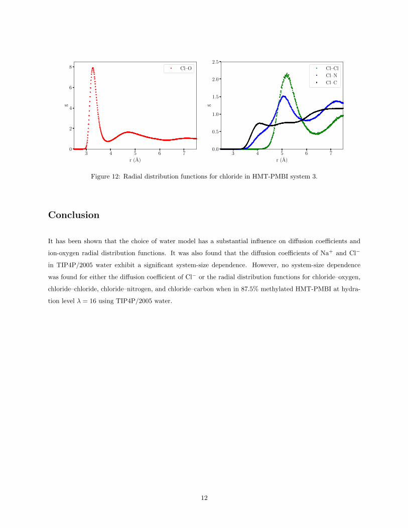
The radial distribution function was calculated using the g(r) tool in VMD for Cl–O, Cl–Cl, Cl–N, and

Cl–C, shown in Fig. 12. The radii of first maximas were measured and uncertainties estimated from the

10

repeats of system 1 as previously mentioned. These radii were plotted as a function of inverse simulation

cell length and fit by least squares with a straight-line. The results are displayed in Table 11. The system

size has no discernible effect on any of the radial distribution functions investigated.

System 1 System 2 System 3 Corrected

Cl–O (A) 3.268 ± 0.003 3.275 ± 0.005 3.265 ± 0.005 3.26 ± 0.014

Cl–Cl (A) 5.19 ± 0.03 5.19 ± 0.05 5.21 ± 0.05 5.2 ± 0.14

Cl–N (A) 5.08 ± 0.014 5.04 ± 0.02 5.04 ± 0.02 4.96 ± 0.06

Cl–C (A) 4.115 ± 0.005 4.065 ± 0.008 4.105 ± 0.008 4.05 ± 0.02

Table 11: Corrected positions of the first maximum for various radial distribution functions.

0 5 10 15 20 25t (ns)

0

100

200

300

400

500

600

MS

D(A

2)

f(t) = 22.728t + 43.45

0 5 10 15 20 25t (ns)

5.0

7.5

10.0

12.5

15.0

17.5

20.0D

(A2/n

s)

Figure 10: Mean squared displacements of chloride in HMT-PMBI system 3 with straight-line fit performed

from 10 ns to 25 ns (left) and associated instantaneous diffusion coefficients (right).

0.0000 0.0025 0.0050 0.0075 0.0100 0.0125 0.0150 0.0175

1/L (A−1)

3.2

3.4

3.6

3.8

4.0

4.2

D(A

2/n

s)

f(1/L) = 20/L + 3.5

Figure 11: Apparent diffusion coefficients for chloride in HMT-PMBI as a function of inverse box length

with straight-line fit.

11

3 4 5 6 7

r (A)

0

2

4

6

8g

Cl–O

3 4 5 6 7

r (A)

0.0

0.5

1.0

1.5

2.0

2.5

g

Cl–Cl

Cl–N

Cl–C

Figure 12: Radial distribution functions for chloride in HMT-PMBI system 3.

Conclusion

It has been shown that the choice of water model has a substantial influence on diffusion coefficients and

ion-oxygen radial distribution functions. It was also found that the diffusion coefficients of Na+ and Cl−

in TIP4P/2005 water exhibit a significant system-size dependence. However, no system-size dependence

was found for either the diffusion coefficient of Cl− or the radial distribution functions for chloride–oxygen,

chloride–chloride, chloride–nitrogen, and chloride–carbon when in 87.5% methylated HMT-PMBI at hydra-

tion level λ = 16 using TIP4P/2005 water.

12

References

1 M. P. Allen and D. J. Tildesley. Computer Simulation of Liquids. Oxford: Clarendon Press, 1989.

2 In-Chul Yeh and Gerhard Hummer. System-size dependence of diffusion coefficients and viscosities from

molecular dynamics simulations with periodic boundary conditions. The Journal of Physical Chemistry

B, 108(40):15873–15879, 2004.

3 In Suk Joung and Thomas E. Cheatham. Molecular dynamics simulations of the dynamic and energetic

properties of alkali and halide ions using water-model-specific ion parameters. The Journal of Physical

Chemistry B, 113(40):13279–13290, 2009.

4 Steve Plimpton. Fast parallel algorithms for short-range molecular dynamics. Journal of Computational

Physics, 117(1):1 – 19, 1995.

5 H. J. C. Berendsen, J. R. Grigera, and T. P. Straatsma. The missing term in effective pair potentials. The

Journal of Physical Chemistry, 91(24):6269–6271, 1987.

6 Hans W. Horn, William C. Swope, Jed W. Pitera, Jeffry D. Madura, Thomas J. Dick, Greg L. Hura, and

Teresa Head-Gordon. Development of an improved four-site water model for biomolecular simulations:

TIP4P-Ew. The Journal of Chemical Physics, 120(20):9665–9678, 2004.

7 J. L. F. Abascal and C. Vega. A general purpose model for the condensed phases of water: TIP4P/2005.

The Journal of Chemical Physics, 123(23):234505, 2005.

8 In Suk Joung and Thomas E. Cheatham. Determination of alkali and halide monovalent ion parameters for

use in explicitly solvated biomolecular simulations. The Journal of Physical Chemistry B, 112(30):9020–

9041, 2008.

9 Kasper P. Jensen and William L. Jorgensen. Halide, ammonium, and alkali metal ion parameters for

modeling aqueous solutions. Journal of Chemical Theory and Computation, 2(6):1499–1509, 2006.

10 L. Martınez, R. Andrade, E. G. Birgin, and J. M. Martınez. PACKMOL: A package for building initial

configurations for molecular dynamics simulations. Journal of Computational Chemistry, 30(13):2157–

2164, 2009.

11 Jean-Paul Ryckaert, Giovanni Ciccotti, and Herman J.C Berendsen. Numerical integration of the carte-

sian equations of motion of a system with constraints: molecular dynamics of n-alkanes. Journal of

Computational Physics, 23(3):327 – 341, 1977.

12 Junmei Wang and Tingjun Hou. Application of molecular dynamics simulations in molecular property

prediction II: Diffusion coefficient. Journal of Computational Chemistry, 32(16):3505–3519, 2011.

13

13 William Humphrey, Andrew Dalke, and Klaus Schulten. VMD: Visual molecular dynamics. Journal of

Molecular Graphics, 14(1):33 – 38, 1996.

14 Toni Giorgino. Computing diffusion coefficients in macromolecular simulations: the Diffusion Coefficient

Tool for VMD. Journal of Open Source Software, 4(41):1698, 2019.

15 David R. Lide, editor. CRC Handbook of Chemistry and Physics. Taylor and Francis Group: Boca Raton,

FL., 87 edition, 2007.

16 Alexander P. Lyubartsev and Aatto Laaksonen. Concentration effects in aqueous nacl solutions. a molec-

ular dynamics simulation. The Journal of Physical Chemistry, 100(40):16410–16418, 1996.

17 Yizhak Marcus. Ionic radii in aqueous solutions. Chemical Reviews, 88(8):1475–1498, 1988.

18 Eric M. Schibli, Jacob C. Stewart, Aidan A. Wright, Binyu Chen, Steven Holdcroft, and Barbara J.

Frisken. The nanostructure of hmt-pmbi, a sterically hindered ionene. Macromolecules, 53(12):4908–4916,

2020.

19 William L. Jorgensen, David S. Maxwell, and Julian Tirado-Rives. Development and testing of the OPLS

all-atom force field on conformational energetics and properties of organic liquids. Journal of the American

Chemical Society, 118(45):11225–11236, 1996.

14