1

The Optimal Power Flow Problem:

Definitions, Solutions, and Challenges Daniel R. Fisher, MSEE Student, University of St. Thomas

in partial fulfillment of

ETLS 747 Electric Machines

Dr. Cal Hardie

Spring 2016

Abstract

Grid level power systems are designed to deliver power from generators to customer

loads as economically as possible while operating within the various equipment constraints (e.g.

transmission line and transformer thermal limits, generator real and reactive power limits,

scheduled tie-line power flows, etc.). This must be managed while simultaneously maintaining

system stability, such as controlling for area frequency, bus voltage magnitudes and phases, and

real and reactive power flows. The problem, called Optimal Power Flow (OPF), has been well

defined since the 1960s but has proven difficult to solve [1]. It is comprised of a coupled system

of non-linear equations for which no exact solution can be found. Instead, iterative algorithms

are employed to solve the problem numerically. For a moderately sized grid, there are typically

hundreds of generators providing power to thousands of buses. Advances in CPU speeds have

enabled faster and more precise numerical solutions, but are still unable to solve the entire

problem quickly enough for certain applications. This project gives an overview of the OPF

problem, defines the important variables and constraints, demonstrates the time required for

solving IEEE test networks using a MATLAB package called MATPOWER, and discusses

methodologies for improving solution times.

2

Introduction

Since the advent of large electrical grids in the first half of the 20th century, system

operators have concerned themselves with providing reliable service to their customers at a

minimum of cost. This involves meeting a varying demand for electricity over the course of each

24-hour period. Multiple generators inject real and reactive power at certain locations (generator

or PV buses) which is sent over transmission lines of varying lengths for customers to receive at

the other ends (load or PQ buses).

Peter Fox-Penner describes the electric power grid in his 2014 book, Smart Power [2],

with a “pond system analogue.” Imagine a network of ponds connected by free flowing channels,

as in Figure 1. The ponds are fed by water towers adding water to the ponds. Simultaneously,

homes draw water out of the ponds for their own use via pipes. At all times, the water added

from the towers must balance the water drawn out by the homes. Otherwise the ponds could

either flood or dry up. Note that the water drawn by one home is not necessarily from one tower,

but instead drawn from the collective contribution of all towers to the pond system.

Figure 1. “Pond system analogue” for the power grid (Fig. 3-1 from Smart Power [2])

3

In the grid, generators act as the water towers, transmission lines are similar to the

interconnecting channels, and customers draw real and reactive power for loads similar to the

homes drawing water from the ponds. However, this balance between generation and load must

be maintained over much smaller time scales than the pond system analogy suggests. At all

moments the power produced by generators must be equal to the power consumed at loads (there

is not often large scale energy storage on the grid like the ponds in the analogy above).

Original operators of early 20th century power grids dealt with this balancing act in a

variety of ad hoc ways. These could involve modeling a power system with a smaller analog

analyzer. Calculations were done on special slide rules. In the end, system adjustments were

often made with a good deal of experienced engineering judgment and intuition.

The problem of optimal power flow was well defined in 1962 [3], but finding a solution

that is fast enough for large power grids remains elusive even today. As we will see, the problem

involves minimizing a non-linear objective function (system cost in $/hr) subject to a large

number of non-linear equality constraints (power flow equations) along with other inequality

constraints (power limitations of generators, transformers and transmission lines). It is a problem

that requires a solution as often as every 5 minutes, accomplished for large systems only through

varying degrees of approximation. More accurate solutions to the optimal power flow problem

could provide an increase in efficiency of 5% for energy markets worldwide, leading to savings

of $19 billion annually in the United States alone [1, p. 5].

This paper will provide an overview of power flow and economic dispatch, then discuss

how they are combined into the optimal power flow (OPF) problem. Finally, various solvers will

be used in MATLAB to illustrate the challenges encountered when trying to solve OPF

problems.

Power Flow

Consider the simple 2-bus system in Figure 2 where the transmission line is modeled as

inductive only.

Figure 2. A simple 2-bus system.

The real and reactive power transmitted to the receiving bus is:

(1)

(2).

We see that the variables related to power flow at each bus are P, Q, voltage magnitude V, and

voltage angle . In order to maintain frequency synchronicity, is kept small. It is important to

note that for small voltage angles, sin ≈ and cos ≈ 1. This fact means that P is closely

𝑃𝑅 =𝑉𝑆𝑉𝑅𝑋

sin 𝛿

𝑄𝑅 =𝑉𝑆𝑉𝑅𝑋

cos 𝛿 −𝑉𝑅2

𝑋

4

coupled to , and Q is closely coupled to V. This will later lead to the decoupling of the P- and

Q-V power flow equations to allow for faster approximate solutions.

For more than two buses, the power flow at each bus is affected by each of the other

interconnected buses. Consider N-buses connected by transmission lines expresses by the

standard bus admittance matrix Ybus. If ymn is the total complex admittance between bus-m and

bus-n, and ymm is the shunt admittance from bus-m to earth ground, then

(3)

(4).

For computation convenience, each element of the Ybus matrix can be expressed in polar form.

(5)

The power flow at the kth bus is then

(6)

(7).

Each bus is specified by 4 variables (P, Q, V, and , but 2 variables are assumed as given

and 2 are unknown. Generators are considered PV-buses where known real power P is injected at

voltage magnitude V, but Q and need to be solved. Loads are expressed as PQ-buses where

known real and reactive power is consumed and and V need to be solved. Finally, one bus is

left as a reference or slack bus where V = 1.0 pu and = 0o (typically), but P and Q need to be

solved to “pick up the slack” of the system. The slack bus is left until the end and simply back-

solved once the other buses are found. We are left with 2(N – 1) non-linear equations to solve for

an equal number of unknown variables. This can be done through various numerical solvers,

among which the Newton-Raphson method is the most common [4].

At this point it is worth noting that the real power set points for each generator in the

network is specified before running the power flow solution (with the exception of the slack

bus). The question remains, which generators should be most utilized to provide power for the

required loads? The answer lies in considering the economics of running each generator.

Economic Dispatch

A system operator must decide what power each generator in the system should provide

in order to meet the ever changing customer demand. However, the power flow equations do not

provide this information. For example, consider the system of Figures 3a and 3b. Both

configurations provide the necessary real and reactive power to the load bus, but which is

Y𝑘𝑘 = ∑𝑦𝑘𝑛

𝑁

𝑛=1

Y𝑘𝑖 = −𝑦𝑘𝑖

Y𝑘𝑛 = 𝑌𝑘𝑛𝑒𝑗𝜃𝑘𝑛

5

favored? The costs associated with running each generator must be included in the decision such

that the system runs at the lowest possible overall cost. This process of finding the lowest cost

configuration is called Economic Dispatch.

Figure 3a. A possible dispatch where each generator carries half the required load.

Figure 3b. Another dispatch where the slack generator provides significantly less than half the real power to the

system.

Each generator has associated with it a cost rate function F(P) expressing the $/hr

required to run the generator as a function of output real power, P. The function can be modeled

in different ways, but is typically either quadratic (as in Figure 4) or piecewise-linear. Generators

have both a maximum and minimum power output Pmin and Pmax ind which they can operate

efficiently.

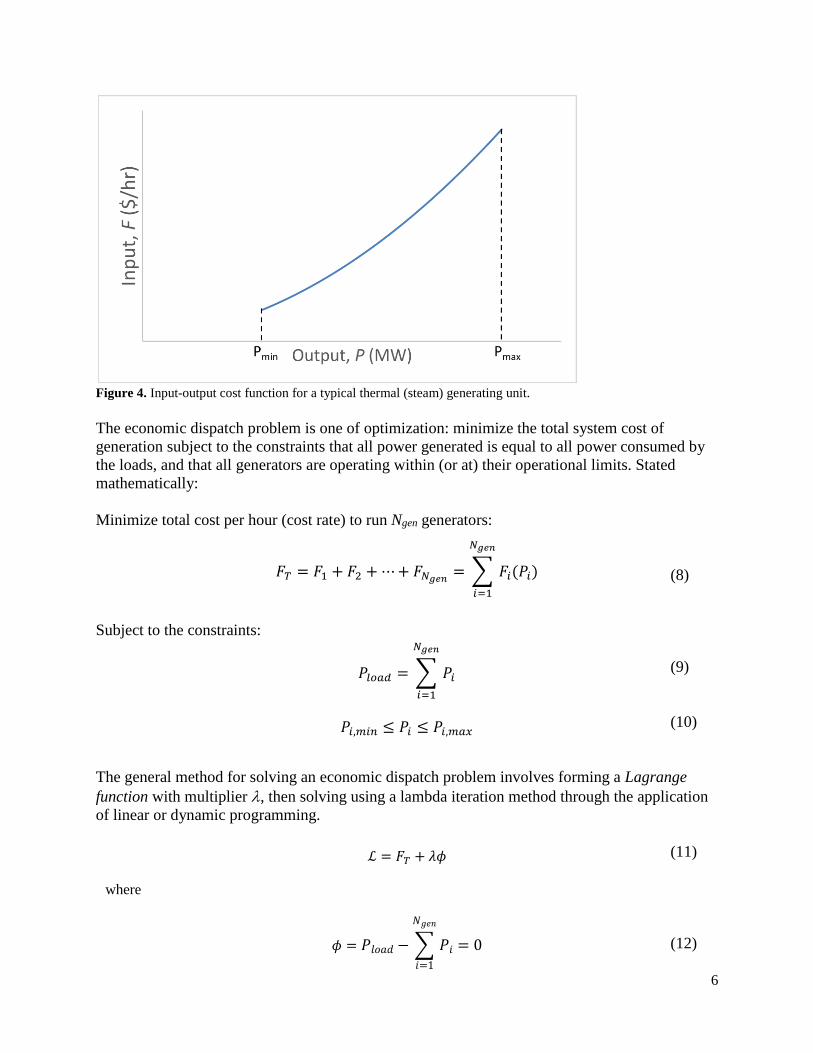
6

Figure 4. Input-output cost function for a typical thermal (steam) generating unit.

The economic dispatch problem is one of optimization: minimize the total system cost of

generation subject to the constraints that all power generated is equal to all power consumed by

the loads, and that all generators are operating within (or at) their operational limits. Stated

mathematically:

Minimize total cost per hour (cost rate) to run Ngen generators:

(8)

Subject to the constraints:

(9)

(10)

The general method for solving an economic dispatch problem involves forming a Lagrange

function with multiplier , then solving using a lambda iteration method through the application

of linear or dynamic programming.

(11)

(12)

𝐹𝑇 = 𝐹1 + 𝐹2 +⋯+ 𝐹𝑁𝑔𝑒𝑛 = ∑ 𝐹𝑖(𝑃𝑖)

𝑁𝑔𝑒𝑛

𝑖=1

𝑃𝑙𝑜𝑎𝑑 = ∑ 𝑃𝑖

𝑁𝑔𝑒𝑛

𝑖=1

𝑃𝑖,𝑚𝑖𝑛 ≤ 𝑃𝑖 ≤ 𝑃𝑖,𝑚𝑎𝑥

ℒ = 𝐹𝑇 + 𝜆𝜙

where

𝜙 = 𝑃𝑙𝑜𝑎𝑑 − ∑ 𝑃𝑖

𝑁𝑔𝑒𝑛

𝑖=1

= 0

7

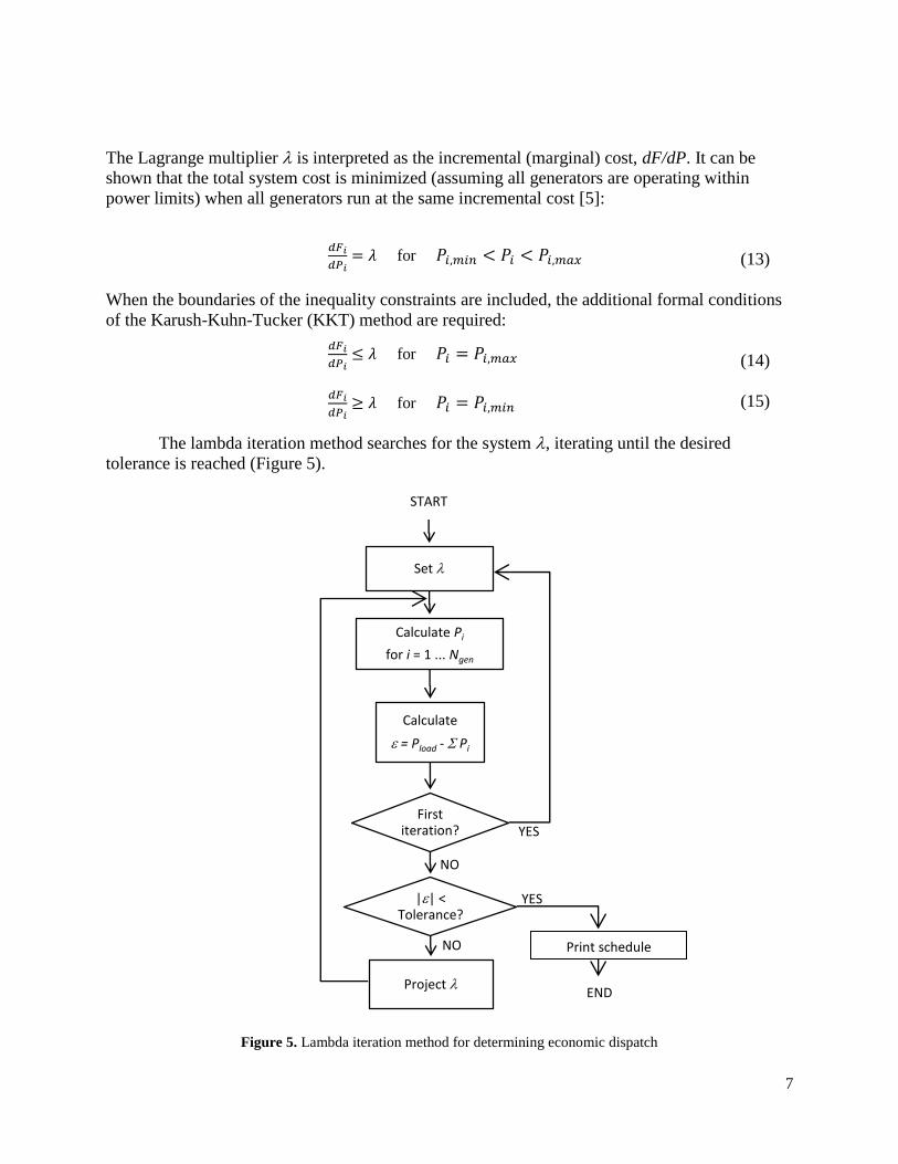
The Lagrange multiplier is interpreted as the incremental (marginal) cost, dF/dP. It can be

shown that the total system cost is minimized (assuming all generators are operating within

power limits) when all generators run at the same incremental cost [5]:

(13)

When the boundaries of the inequality constraints are included, the additional formal conditions

of the Karush-Kuhn-Tucker (KKT) method are required:

(14)

(15)

The lambda iteration method searches for the system , iterating until the desired

tolerance is reached (Figure 5).

Figure 5. Lambda iteration method for determining economic dispatch

START

Set

Calculate Pi

for i = 1 ... Ngen

Calculate

e = Pload - S Pi

First iteration?

|e| < Tolerance?

Project

𝑑𝐹𝑖

𝑑𝑃𝑖= 𝜆 for 𝑃𝑖,𝑚𝑖𝑛 < 𝑃𝑖 < 𝑃𝑖,𝑚𝑎𝑥

𝑑𝐹𝑖

𝑑𝑃𝑖≤ 𝜆 for 𝑃𝑖 = 𝑃𝑖,𝑚𝑎𝑥

𝑑𝐹𝑖

𝑑𝑃𝑖≥ 𝜆 for 𝑃𝑖 = 𝑃𝑖,𝑚𝑖𝑛

Print schedule

END

YES

NO

NO

YES

8

Optimal Power Flow

Optimal power flow seeks to minimize the total system cost function FT, while at the

same time solving the system power flow. Since the transmission line admittances are built into

the power flow solution there is no need to separately consider losses when solving for economic

dispatch. Summarizing the OPF problem:

Minimize the total system generation cost FT (Eqn. 8)

Include generator limit inequality constraints for real and reactive power (Eqn. 10 and

similar for reactive power, Qi,min ≤ Qi ≤ Qi,min)

Include transmission system thermal inequality constraints, expressed as either apparent

power or effective current limits for lines and transformers

Include bus voltage magnitude inequality constraints, Vi,min ≤ Vi ≤ Vi,min

Include equality constraints for real and reactive power flow (Eqns. 6 and 7)

This problem is LARGE, requiring the repeated solving of 2(N – 1) nonlinear equations

while trying to optimize (minimize) an objective function subject to a large number of

constraints. A moderately sized power system can have thousands of voltage buses with

hundreds of generating units. For large grids the buses number in the tens of thousands. Couple

this with the need to solve for OPF repeatedly to economically schedule generators for a

constantly changing demanded load. The more often OPF needs to be solved, the less time there

is to solve it. It must be solved [1]:

Weekly in 8 hrs

Daily in 2 hrs

Hourly in 15 min

Every 5 min in 1 min

Perhaps every 30s as we move toward “self-healing” smart grids

Despite the fact that computation speeds have increased by a factor of 107 over the 20

years leading up to 2012 [1], modern computers are still not fast enough to solve the full OPF

problem as often as it is needed. As such, approximate models are employed. Most common is

the so-call “DC” OPF.

Simplifications required for DCOPF solutions:

Decouple P and V, and Q and . As was noted following Eqns. 1 and 2, for small voltage

angles real power is primarily affected by voltage angles, and reactive power is primarily

affected by voltage magnitudes. By neglecting the all the partial derivatives in the

Jacobian matrix (required in the Newton-Raphson method) of the form 𝜕𝑃𝑘/𝜕𝑉𝑖 and

𝜕𝑄𝑘/𝜕𝛿𝑖, the power flow equations are formulated as two decoupled equations, namely

the P – and Q – V equations.

Use small angle approximations for sine and cosine functions.

Assume all voltage magnitudes are constant, Vi = 1.0 pu.

To clarify, we are still dealing with a balanced 3-phase AC system. But because the

voltage magnitudes are assumed constant, the system has fixed, or “DC”, voltage. The DCOPF

approximation results in a single linear matrix equation with a straightforward non-iterative

9

solution. While this approximate solution is significantly faster than the full ACOPF, it is limited

to real (MW) power information, since the reactive power is completely neglected.

The full ACOPF has about twice as many variables as the DCOPF formulation.

Furthermore, the ACOPF network equations are non-linear, making it much more difficult to

reliably solve. It can be approached by solving an initial power flow and using it as an operating

point Pgen0, Qgen

0, V0 and 0 about which the objective function and constraints are linearized.

Then the techniques of linear programming (the details of which are not covered in this paper)

can be used to iterate towards a solution.

Steps for the incremental linear programming (LP) solution to the ACOPF [5, p. 372]:

1) Solve a base power flow

2) Linearize the objective function

3) Linearize the constraints (including power flow equations with full Jacobian matrix)

4) Set variable limits

5) Solve the LP

6) Check P, Q, V tolerances and go to step 1 at a new operating point as necessary

Comparison of OPF Solutions

MATPOWER is a package of MATLAB M-files for solving power flow and optimal

power flow problems. It is intended as a simulation tool for researchers and educators that is easy

to use and to modify [6, 7]. Included in the package are a set of sample cases which allow for the

comparison of DCOPF and ACOPF solutions. Figures 6, 7, and 8 show a summary of

convergence times for a series of test cases performed on the author’s laptop, followed by the

MATPOWER summary of the largest included case (case9241pegase.m) for both the DCOPF

and ACOPF solvers.

Figure 6. Comparison of MATPOWER convergence times for DCOPF and ACOPF of test case networks.

Case Nbuses Ngenerators Nloads DCOPF (s) ACOPF (s) % Increase

case118 118 54 99 0.07 0.14 200

case300 300 69 201 0.20 0.24 120

case1354pegase 1354 260 673 0.70 2.15 307

case2869pegase 2869 510 1485 1.63 4.99 306

case3120sp 3120 505 2277 4.51 5.63 125

case9241pegase 9241 1445 4895 1.68 22.13 1317

10

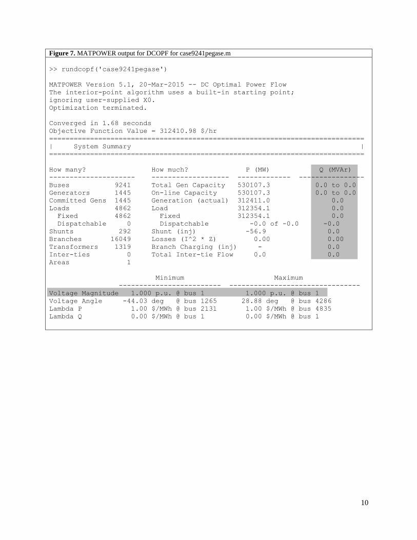
Figure 7. MATPOWER output for DCOPF for case9241pegase.m

>> rundcopf('case9241pegase')

MATPOWER Version 5.1, 20-Mar-2015 -- DC Optimal Power Flow

The interior-point algorithm uses a built-in starting point;

ignoring user-supplied X0.

Optimization terminated.

Converged in 1.68 seconds

Objective Function Value = 312410.98 $/hr

=============================================================================

| System Summary |

=============================================================================

How many? How much? P (MW) Q (MVAr)

--------------------- ------------------- ------------- ----------------

Buses 9241 Total Gen Capacity 530107.3 0.0 to 0.0

Generators 1445 On-line Capacity 530107.3 0.0 to 0.0

Committed Gens 1445 Generation (actual) 312411.0 0.0

Loads 4862 Load 312354.1 0.0

Fixed 4862 Fixed 312354.1 0.0

Dispatchable 0 Dispatchable -0.0 of -0.0 -0.0

Shunts 292 Shunt (inj) -56.9 0.0

Branches 16049 Losses (I^2 * Z) 0.00 0.00

Transformers 1319 Branch Charging (inj) - 0.0

Inter-ties 0 Total Inter-tie Flow 0.0 0.0

Areas 1

Minimum Maximum

------------------------- --------------------------------

Voltage Magnitude 1.000 p.u. @ bus 1 1.000 p.u. @ bus 1

Voltage Angle -44.03 deg @ bus 1265 28.88 deg @ bus 4286

Lambda P 1.00 $/MWh @ bus 2131 1.00 $/MWh @ bus 4835

Lambda Q 0.00 $/MWh @ bus 1 0.00 $/MWh @ bus 1

11

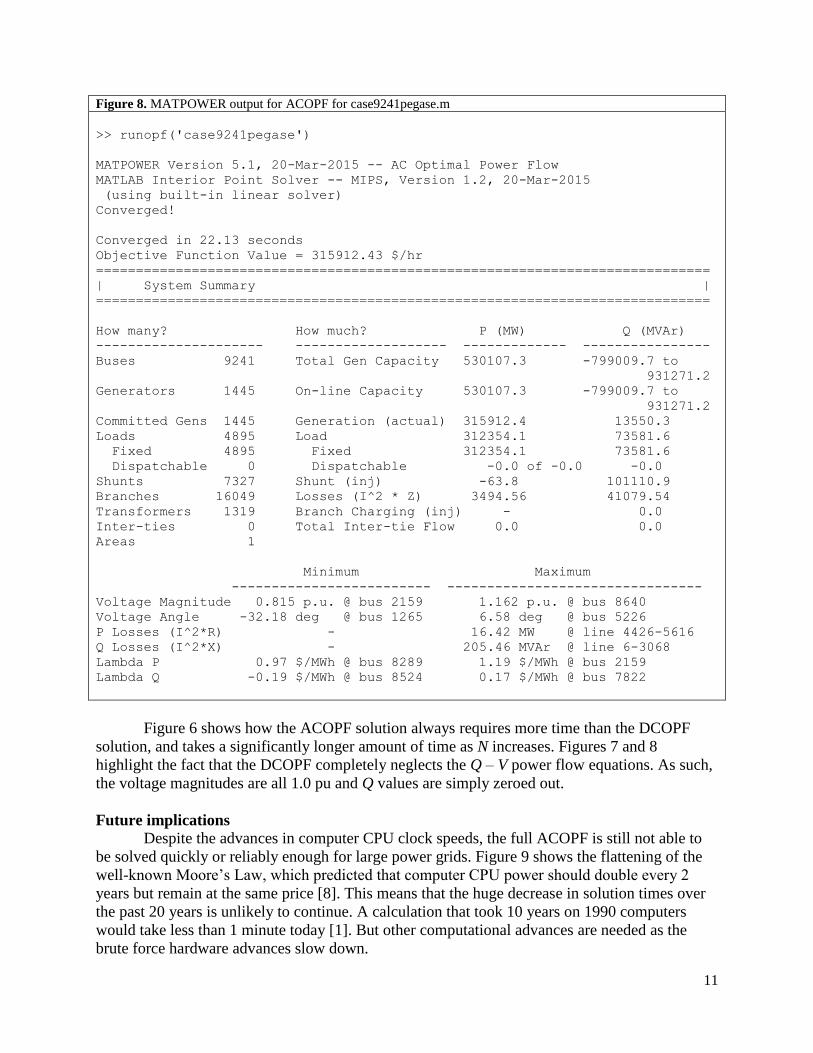
Figure 8. MATPOWER output for ACOPF for case9241pegase.m

>> runopf('case9241pegase')

MATPOWER Version 5.1, 20-Mar-2015 -- AC Optimal Power Flow

MATLAB Interior Point Solver -- MIPS, Version 1.2, 20-Mar-2015

(using built-in linear solver)

Converged!

Converged in 22.13 seconds

Objective Function Value = 315912.43 $/hr

=============================================================================

| System Summary |

=============================================================================

How many? How much? P (MW) Q (MVAr)

--------------------- ------------------- ------------- ----------------

Buses 9241 Total Gen Capacity 530107.3 -799009.7 to

931271.2

Generators 1445 On-line Capacity 530107.3 -799009.7 to

931271.2

Committed Gens 1445 Generation (actual) 315912.4 13550.3

Loads 4895 Load 312354.1 73581.6

Fixed 4895 Fixed 312354.1 73581.6

Dispatchable 0 Dispatchable -0.0 of -0.0 -0.0

Shunts 7327 Shunt (inj) -63.8 101110.9

Branches 16049 Losses (I^2 * Z) 3494.56 41079.54

Transformers 1319 Branch Charging (inj) - 0.0

Inter-ties 0 Total Inter-tie Flow 0.0 0.0

Areas 1

Minimum Maximum

------------------------- --------------------------------

Voltage Magnitude 0.815 p.u. @ bus 2159 1.162 p.u. @ bus 8640

Voltage Angle -32.18 deg @ bus 1265 6.58 deg @ bus 5226

P Losses (I^2*R) - 16.42 MW @ line 4426-5616

Q Losses (I^2*X) - 205.46 MVAr @ line 6-3068

Lambda P 0.97 $/MWh @ bus 8289 1.19 $/MWh @ bus 2159

Lambda Q -0.19 $/MWh @ bus 8524 0.17 $/MWh @ bus 7822

Figure 6 shows how the ACOPF solution always requires more time than the DCOPF

solution, and takes a significantly longer amount of time as N increases. Figures 7 and 8

highlight the fact that the DCOPF completely neglects the Q – V power flow equations. As such,

the voltage magnitudes are all 1.0 pu and Q values are simply zeroed out.

Future implications

Despite the advances in computer CPU clock speeds, the full ACOPF is still not able to

be solved quickly or reliably enough for large power grids. Figure 9 shows the flattening of the

well-known Moore’s Law, which predicted that computer CPU power should double every 2

years but remain at the same price [8]. This means that the huge decrease in solution times over

the past 20 years is unlikely to continue. A calculation that took 10 years on 1990 computers

would take less than 1 minute today [1]. But other computational advances are needed as the

brute force hardware advances slow down.

12

Figure 9. Moore’s Law has failed to predict CPU advances over the past 10 years as new chips have proven more

expensive and more difficult to cool. [8]

The problem is highlighted when looking at DCOPF and ACOPF solution times from

larger grids. Figure 10 shows convergence times for various test networks over a range

algorithm-based solvers implemented in MATLAB [7]. Note that for the largest 42k-bus

networks, the fastest full ACOPF solution took over an hour. In security-constrained studies,

where engineers are studying the effects of losing various system elements, repeated ACOPF

solutions are required. Clearly, waiting an hour for each one becomes unwieldy. Furthermore, as

more grids implement “smart switching” equipment, OPF solutions will be needed more quickly

as the system automatically adapts to changes.

Figure 10. Comparison of solution times for various test networks, implemented in MATLAB. Note that case42k

required at least 3,700 s = 61.7 min to find a single full ACOPF solution [7].

13

With individual CPU clock speeds remaining more or less constant, ACOPF solutions

that leverage parallel computing are being developed. In a 2013 industry white paper [9], FERC

states that there is “a clear advantage to employing a multistart strategy, which leverages parallel

processing in order to solve the ACOPF on large-scale networks for time-sensitive applications.”

A multistart strategy is “a global optimization procedure that applies a solution technique for

numerous starting points on parallel threads/processes and then terminates with increasing

confidence in a unique optimal solution.” These types of parallel computing strategies are easily

scalable ad hoc with available cloud computing resources.

Other research efforts are underway to find more robust solving algorithms which more

reliably converge to an optimal solution. One such paper [10] reformulates the ACOPF problem

based on a current injection approach that linearly couples the quadratic constraints at each bus.

This results in a set of linear equations rather than a set of coupled non-linear equations (Eqns. 6

and 7). These are then solved with a successive linear programming (SLP) algorithm. It was

shown that these performed favorably when compared to the best non-linear programming (NLP)

approaches.

Conclusion The Optimal Power Flow problem remains a challenge for power systems operators. The

OPF problem seeks to find a generator dispatch schedule that both minimizes the total system

cost while simultaneously satisfying the constraints imposed by transmission power flows and

component limits. A faster, more robust solution to this problem will mean savings of billions of

dollars annually. Currently, many time-sensitive applications rely on the faster approximate

DCOPF solutions which can be unsuitable for tightly coupled power systems. However,

researchers in optimization algorithms hope to achieve faster solutions to the full ACOPF

problem. This will enable the development of “smart grid” implementations with their self-

healing switching schemes. Perhaps growing resources available through scalable cloud

computing will be the key. Only time will tell.

References

[1] M. B. Cain et al., “History of Optimal Power Flow and Formulations,” FERC, 2012.

Available: http://www.ferc.gov/industries/electric/indus-act/market-planning/opf-papers/acopf-1-

history-formulation-testing.pdf

[2] P. Fox-Penner, “The New Paradigm,” in Smart Power, 2nd ed.. Washington DC: Island

Press, 2014.

[3] J. Carpentier, “Contribution á l’étude du dispatching économique,” Bulletin de la Société

Française des Électriciens, ser. 8, vol. 3, pp. 431-447, 1962.

[4] J. D. Glover et al., “Power Flows” in Power Systems Analysis and Design, 5th ed. Stamford:

Cengage Learning, 2012, ch. 6, sec. 6, pp. 334-343.

[5] A. J. Wood et al., “Economic Dispatch of Thermal Units and Methods of Solution” in

Power Generation, Operation, and Control, 3rd ed. Hoboken: John Wiley & Sons, Inc., 2014,

ch. 3, pp. 63-146.

14

[6] R. D. Zimmerman and C. E. Murillo-Sánchez, (2016, May 14). MATPOWER: A MATLAB

Power System Simulation Package. [Online]. Available: http://www.pserc.cornell.edu/matpower/

[7] R. D. Zimmerman, C. E. Murillo-Sánchez, and R. J. Thomas, "MATPOWER: Steady-State

Operations, Planning and Analysis Tools for Power Systems Research and Education," Power

Systems, IEEE Transactions on, vol. 26, no. 1, pp. 12-19, Feb. 2011.

[8] T. Cross, (2016, March 12). Technology Quarterly: After Moore’s Law. [Online]. Available:

http://www.economist.com/technology-quarterly/2016-03-12/after-moores-law

[9] A. Castillo and R. P. O’Neill, “Computational Performance of Solution Techniques Applied

to the ACOPF,” FERC, 2013. Available: http://www.ferc.gov/industries/electric/indus-

act/market-planning/opf-papers/acopf-5-computational-testing.pdf

[10] A. Castillo et al., “A Successive Linear Programming Approach to Solving the IV-

ACOPF,” Power Systems, IEEE Transactions on, vol. 31, no. 4, pp. 2752-2763, July 2016.