development of traffic data input resources for the ... · xi the cleaned data are then processed...

Development of Traffic Data Input Resources for the Mechanistic Empirical Pavement Design Process

Prepared by:

John R. Stone, PhD, Youngsoo R. Kim, PhD, George F. List, PhD, William Rasdorf, PhD, Fatemeh Sayyady, Fadi Jadoun, and Aditya N. Ramachandran

Department of Civil, Construction, and Environmental Engineering North Carolina State University

Raleigh, NC27695-7908

Prepared for:

North Carolina Department of Transportation Transportation Survey Unit

Raleigh, NC27699-1557

Final Report Project: HWY-2008-11

December 1, 2011

Technical Report Documentation Page

Report No. FHWA/NC/2008-11

Government Accession No.

Recipient’s Catalog No.

4. Title and Subtitle Development of Traffic Data Input Resources for the Mechanistic Empirical Pavement Design Process

Report Date December12, 2011

Performing Organization Code

Author(s) John R. Stone, Youngsoo R. Kim, George F. List, William Rasdorf, Fadi, Fatemeh Sayyady, Jadoun, Aditya N. Ramachandran

Performing Organization Report No.

Performing Organization Name and Address North Carolina State University Department of Civil, Construction and Environmental Engineering 208 Mann Hall Raleigh, NC27695-7908

Work Unit No. (TRAIS)

Contract or Grant No.

Sponsoring Agency Name and Address North Carolina Department of Transportation Transportation Planning Branch 1 South Wilmington Street Raleigh, North Carolina27601

Type of Report and Period Covered Final Report July 2007 to August 2010

Sponsoring Agency Code 2008-11

Supplementary Notes:

Abstract The Mechanistic-Empirical Pavement Design Guide (MEPDG) for New and Rehabilitated Pavement Structures uses nationally based data traffic inputs and recommends that state DOTs develop their own site-specific and regional values. To support the MEPDG NCDOT needs site-specific truck classification counts, truck axle load spectra, regional average seasonal adjustment factors, and forecasting methods for truck class volumes. This research proposal addresses these NCDOT traffic data and forecasting needs for implementing the MEPDG. The research produced the following results: (1) software to process and clean WIM data; (2) database of high quality, clean NCDOT vehicle class counts and weight data; (3) simulation studies to guide the selection of sensitive traffic data and traffic count locations; (4) techniques for traffic data clustering and seasonal analysis of vehicle classification and truck axle loadings; (5) software to prepare datasets and sampling plans for Levels 1, 2, and 3 MEPDG requirements (Level 1 site specific, Level 2 seasonal groupings, and Level 3 statewide averages); (6) site specific, regional and statewide NC traffic data inputs for Levels 1, 2, and 3 in the MEPDG procedures for vehicle class distributions and axle load spectra including seasonality; (7) vehicle class forecasting methods for MEPDG procedures; (8) case study demonstrations and analyses; and (9) implementation and management plan for MEPDG traffic data.

Key Words Pavement Design, Traffic Data, Traffic Data Analysis, Damage-based Sensitivity Analysis, Weight-in-Motion Data.

Distribution Statement

Security Classif. (of this report) Unclassified

Security Classif. (of this page) Unclassified

No. of Pages 257

Price

Form DOT F 1700.7 (8-72) Reproduction of completed page authorized

v

DISCLAIMER

The contents of this report reflect the views of the authors and not necessarily the views of the North Carolina State University. The authors are responsible for the facts and the accuracy of the data presented herein. The contents do not necessarily reflect the official views or policies of the North Carolina Department of Transportation or the Federal Highway Administration at the time of publication. This report does not constitute a standard, specification, or regulation.

vi

ACKNOWLEDGEMENTS

The research team acknowledges the North Carolina Department of Transportation for supporting and funding this project. We extend our thanks to the NCDOT Research Project Steering Committee and NCDOT staff, who provided valuable advice and data for the project. They are: Kent Taylor PE, Chair Judith Corley-Ley PhD, PE Stephen Piotrowski Deborah Hutchings, PE Mehdi Haeri Clark Morrison, PhD, PE NjorgeWainaina, PE C.K. Su Jack Cowsert, PE Jim Phillips, PE Todd Whittington, PE The authors especially appreciate the contributions and hard work of staff at Traffic Survey Group (TSG) at NCDOT. Particular thanks are due to Kent Taylor for his valuable guidance during the project. The authors also extend special thanks to Soheil Sajjadi, a Ph.D. student at NCSU, who helped clean the data and support other tasks. The authors also acknowledge and appreciate the educational funding from the Southeastern Transportation Center. Without this special funding components of the research may not have been completed.

vii

ACRONYMS Acronym

Meaning

AADTT Annual Average Daily Truck Traffic AADT Annual Average Daily Traffic ADT Average Daily Traffic ALDF Axle Load Distribution Factors APT Axles per Truck AASHTO American Association of State Highway and Transportation Officials BY Base Year CRCP Continuously Reinforced Concrete Pavement DOW Day of Week DDF Directional Distribution Factor FHWA Federal Highway Administration FC Functional Class FY Future Year HDF Hourly Distribution Factors HPMS Highway Performance Monitoring System IRD International Road Dynamics IRI International Roughness Index JPCP Jointed Plain Concrete Pavement (JPCP) LDF Lane Distribution Factor LTPP Long Term Pavement Performance MAF Monthly Adjustment Factors MADTT Monthly Average Day-of-week Truck Traffic MEPDG Mechanistic Empirical Pavement Design Guide MU Multi-Unit Trucks (Vehicle Classes 8-13) NCSU North Carolina State University PC Principal Component PCA Principal Component Analysis PDU Pavement Design Unit SU Single-Unit Trucks (Vehicle Classes 4-7) TFU Traffic Forecasting Utility TPB Transportation Planning Branch TPB/TF Transportation Planning Branch/Traffic Forecast TMG Traffic Monitoring Guide TSG Traffic Survey Group VCD Vehicle Class Distribution VTRIS Vehicle Travel Information System WIM Weigh-in-Motion

ix

EXECUTIVE SUMMARY The Mechanistic Empirical Pavement Design Guide (MEPDG) requires specific types of traffic data to design new or rehabilitated pavement structures (1). Among the required data are axle load distribution factors (ALDF), monthly adjustment factors (MAF), hourly distribution factors (HDF), and vehicle class distributions (VCD). For each of these four factors depending on the level of design the MEPDG requires traffic distributions for each of 10 standard FHWA vehicle classes (4-13). The design levels are:

Level 1: most accurate design level requiring site-specific weight and volume data collected at or near the project site.

Level 2: intermediate accuracy design level with modest knowledge of traffic characteristics requiring regional weight data and site-specific volume data.

Level 3: least accurate design level with knowledge only of statewide default weight and volume data.

Analyzing Level 1 data is straightforward. The difficulties lie in generating Level 2 data that pertain to roadways with limited traffic information. Level 3 analysis is an extension of the Level 2 analysis. Other states have also studied the problem of characterizing the truck traffic for Mechanistic-Empirical (M-E) pavement design [Prozzi, 2005,Lu et al,. 2006, Papagiannakis (a),2006, Timm et a., 2006, Tran and Hall, 2007, Li et al., 2007, Swan et al., 2008, Lu et al., 2009]. Table 1 shows the traffic data elements required for different design levels.

Table 1 Traffic Data Elements Required for the MEPDG

Traffic Data Element

Annual Average Daily Truck Traffic Monthly Adjustment Factors by Vehicle Class Hourly Distribution Factors Vehicle Class Distribution Factors Axle-Load Distribution Factors Linear or Exponential Growth Rates Directional Distribution Factors Lane Distribution Factors Lateral Traffic Wander Number of Axles per Vehicle for Vehicle Classes 4-13 Axle Configurations Wheelbase Distributions Operational Speed

Figure 1 shows an Input-Process-Output model of this research project that concerns generating Level 2 MEPDG traffic inputs. NCDOT operates 44 WIM sites including 19 Long Term Pavement Performance (LTPP) stations. These WIM sites are located in three regions: the eastern coastal plain, central Piedmont, and western mountains. NCDOT provided twelve consecutive months of calibrated volume and weight data for each WIM site. Initially, the data were checked for completeness and anomalies using a quality control (QC) procedure. The quality control procedure confirmed that the data were reliable [Ramachandran et al., 2010].

x

* A list of acronyms is included in Appendix 1.

Figure 1 Input-Process-Output Model of the Project

NCSU*

• Developing WIM data quality control procedure (Ch 2)• Developing traffic volume adjustment factors – VCD, MAF, and

HDF (Chs 3 and 4)• Developing general traffic inputs (Ch 4)• Proposing traffic data forecasting procedure (Ch 5)• Generating ALDF distributions (Ch 6)• Developing axle load damage factors (Ch 7)• Performing damage-based sensitivity analysis (Ch 8)• Proposing seasonal sampling plan (Ch 9)• Proposing locations to install future WIM stations (Ch 10)

• WIM Data Quality Control Procedure• SU/MU Seasonal Factors• Seasonal Factor Decision Tree• Hourly Distribution Factor (Table 4-1)• Monthly Adjustment Factor (Table 4-2)• Number of Axle per Vehicle Class (Table 4-3)• Lateral Traffic Wander• Axle Configurations (default)• Axle Spacing (Table 4-4)• Wheelbase Distribution• Directional Distribution Factor (default)• Lane Distribution Factor (default)• Operational Speed (default)• Recommendations regarding Traffic Forecasting• ALDF Distributions• ALDF Decision Tree• Seasonal Sampling Procedure• Recommendations regarding Locations of New WIM Stations

WIM data (W-cards and C-cards)

xi

The cleaned data are then processed using computer programming to generate traffic factors including traffic volume adjustment factors (including VCD, HDF, and MAF), ALDF, and general traffic inputs. Traffic Volume Adjustment Factors

The NC State University research team performed MEPDG damage-based sensitivity analysis to identify factors that affect North Carolina pavement performance measures (sensitive factors) and factors that do not (non-sensitive factors). Performance measures for flexible pavements are rutting, alligator cracking, longitudinal cracking, and the International Roughness Index (IRI). For rigid pavements, only Jointed Plain Concrete Pavement (JPCP) is considered because Continuously Reinforced Concrete Pavement (CRCP) is being phased out from use in the North Carolina road network. The performance measures for JPCP are faulting, percentage of slabs cracked, and the IRI. Structural and materials data were available only for LTPP sections. Representative LTPP sections were used in this sensitivity analysis. Representative LTPP sections were used in this sensitivity analysis. To evaluate whether or not the effect of different traffic factors on pavement performance is significant, damage-based sensitivity criteria were developed in cooperation with the North Carolina Department of Transportation (NCDOT). These criteria suggest that an IRI of 14 inches/mile is the limit between being significant and insignificant for both flexible and rigid pavements. Similarly, the limits are 0.1 inch for rutting, 1% of the lane area for alligator cracking, 264 feet/mile for longitudinal cracking, 0.1 inch for JPCP faulting, and 3% for slabs cracked. Table 2 shows the results of the sensitivity analysis. The results of the sensitivity analysis identified pavement performance to be sensitive to VCD. The VCD represents the percentage of each standard FHWA vehicle classes (class 4 buses through class 13 trucks). Table 3 lists the entire 13 standard FHWA vehicle classes. The proposed approach to generate VCD inputs is based on using the site-specific 48-hour vehicle classification counts plus a seasonal factoring procedure that accounts for day-of-week and seasonal variations in truck traffic volume. This simplified approach results in accurate VCD inputs because it incorporates site-specific knowledge of truck traffic. Two types of traffic time distribution factors are needed as inputs. These factors are monthly adjustment factors (MAF) and hourly distribution factors (HDF). Monthly or seasonal distribution factors are used to adjust the Annual Average Daily Truck Traffic (AADTT) into monthly Average Daily Truck Traffic (ADTT) values/volumes, while the hourly distribution factor is used to distribute the monthly ADTT volumes by hour of the day. These time-dependent distribution factors are determined from detailed studies of WIM data. In addition, these factors are treated as constant throughout the pavement design life. The monthly adjustment factor (MAF) is defined as the ratio of the monthly truck volume to the average monthly truck volume. MEPDG damage-based sensitivity analysis showed that pavement performance is not sensitive to NC site-specific and national default values of MAF, thus MAF statewide averages maybe used as input to MEPDG for Level 2 and Level 3 designs. The hourly distribution factors (HDF) represent the percentage of the AADTT within each hour of the day. Based on the damage-based sensitivity analysis, flexible and rigid pavement performance was found to be relatively insensitive to different distributions of HDF. Thus, HDF statewide averages may be used for Level 2 design. Similar results are found when comparing the impact on pavement performance of national default values of HDF. This is a valuable finding that simplifies the design process. The pavement designer can use the HDF statewide averages for Level 2 and Level 3 designs.

xii

Table 2 Sensitivity of Flexible and Rigid Pavements to Different Traffic Parameters

Flexible Pavement Rigid Pavement (JPCP)

Total Rut Depth (in)

Fatigue Cracking (%)

Longitudinal Cracking* (ft/mile)

IRI (in/mile)

Faulting(in)

Slabs Cracked (%)

IRI (in/mile)

HDF × × × × × × ×

MAF × × × × × ×

VCD × ×

ALDF × × ×

* The longitudinal cracking predictions obtained from the MEPDG are inaccurate, hence, the exclusion from the sensitivity study.

Table 3 FHWA Vehicle Classes

Vehicle Class

Number.

Standard FHWA Vehicle Classes

1 Motorcycles

2 Passenger Cars

3 4-tire trucks

4 Buses

5 2-axle 6-tire trucks

6 3-axle trucks

7 4+ axle trucks

8 3-4 axle single-trailer combinations

9 5-axle single-trailer combinations

10 6+ axle single-trailer combinations

11 5-axle multi-trailer combinations

12 6-axle multi-trailer combinations

13 7+ axle multi-trailer combinations

Axle Load Distribution Factor

The ALDF represents the frequency of individual load intervals, known as load bins, for four axle types: single, tandem, tridem, and quad. The single load bins range from 2 – 41 kips at 1-kip interval, the tandem load bins range from 6 – 82 kips at 2- kip interval, and tridem and quad load bins range from 12 – 102 kip sat 3-kip interval. Flexible pavement performance was found to be sensitive to ALDF. After running the MEPDG for a 30-year design life for all rigid pavements, it was found that ALDF has an effect on % slabs cracked of rigid pavement from a "numbers point of view". However, from an "engineering point of view", this change is considered to be insignificant because of the following reason. Only one site out of four sites exhibited the effect of ALDF on % slabs cracked to be higher than the specified thresholds. When looking into the numbers, it was found that the predicted % slabs cracked for this particular site was 3.1% compared to the sensitivity criterion of 3.0%. Again, using engineering

xiii

judgment, the team assumed that a 0.1% difference in % Slabs cracked is not enough to justify that ALDF significantly affects rigid pavements. To develop ALDF inputs the NC State team followed the traditional approach based on inferring traffic data for roadway segments with data deficiencies from WIM data collected at other roads. Given the 44 NCDOT WIM databases available, investigating each database was not practical. Therefore, the team used a multidimensional clustering approach to cluster WIM sites that considers similarity of multiple attributes simultaneously and generates clusters for which their distinctions can be easily explained [Sayyady et al., 2011]. In order to decide what axle types and load combinations to include in multidimensional ALDF clustering, it is important to investigate the frequency and the effect of different axle types on pavement performance. MEPDG damage-based analysis showed that the contribution of tridem and quad axles to pavement damage is not appreciable in North Carolina (both less than 1%) while the effect of single and tandem axles is considerable (35% and 64%, respectively). Furthermore, single and tandem axles are more frequent (57.7% and 41.9%) and they are more representative of traffic on roadways compared to infrequent tridem and quad axles (0.3%, and 0.1%). More specifically, single and tandem axles are more frequent than tridem and quad axles. Given the aforementioned considerations, MEPDG damage analysis demonstrated that single and tandem axles are the two dimensions of the clustering analysis to use and to ignore infrequent tandems and quads. Two-dimensional clustering analysis generates representative ALDF clusters that can be examined to identify explanatory traffic parameters for similar traffic patterns elsewhere on the highway system where design roads are located and for which there are only 48-hour counts. The traffic explanatory parameters define a decision tree to help the pavement engineer select the right ALDF input for the mechanistic-empirical pavement design at the design location. These parameters include 48-hour classification counts that specify design location AADTT and the percentage of class 5 and class 9 vehicles. The design engineer will also be familiar with local economic activities and the highway functional classification at the design location. The explanatory parameters are easy to acquire and result in a decision tree that is sound and straightforward to use. General Traffic Inputs

Besides traffic volume adjustment factors and ALDF, there are some general traffic inputs to MEPDG software including lateral traffic wander, number of axles per truck for each vehicle class, axle configurations, and wheelbase. National default values are recommended for lateral traffic wander input including mean wheel location (in inches from the lane marking), traffic wander standard deviation (in inches), and the design lane width (in feet). These factors were not evaluated in this research. The NCSU team proposes using statewide average number of axles per truck as input to MEPDG. Since different types of vehicles with different axle configurations might be grouped under the same class, this can cause the average number of axle types per vehicle class to appear as a fraction. Regarding axle configurations, the team recommends using national default inputs for average axle widths, dual tire spacing, and tire pressure. Statewide average axle spacing for tandem, tridem and quad axles are derived from available WIM data and are recommend to be used as input to MEPDG. The wheelbase refers to the spacing between the steering and the drive axles of the truck-tractors or heavy single-units. Wheel base distribution information (average axle spacing and percentage of truck for short,

xiv

medium and long axles) is required for JPCP top-down cracking considerations. National default inputs are recommended for wheelbase distribution information. The generated traffic factors along with other data including climatic changes, material and soil properties, and pavement design features are used as input data for M-E pavement design. Seasonal Sampling Plan

Resource and budget constraints may restrict department of transportation from collecting and reporting complete data. Technical problems may produce incomplete or intermittent Weigh-In-Motion (WIM) data. To address these issues WIM data sampling procedures are proposed. The proposed sampling schemes have two dimensions: the frequency (annual, semiannual, quarterly, and monthly) and the duration of samples (2-consecutive weekdays and 5-consecutive weekdays). As discussed above North Carolina pavement performance is sensitive to NC site-specific VCD and ALDF. The procedure to estimate VCD involves annualizing 48-hour counts using proper seasonal factors; hence, it is not necessary to investigate the effect of WIM data sampling plans on VCD estimates. This study focuses on axle load distributions and how effective the sampling procedures are to estimate the ALDF accurately. To evaluate the effectiveness of sampling schemes, the estimates of ALDF derived from WIM data collected over short periods of time are compared to estimates of ALDF derived from annual WIM data. Findings show that there is a direct correlation between seasonal variation of truck traffic and the accuracy of the sampling schemes. As expected, where truck traffic is stable (Piedmont region) all sampling schemes are attractive. Where truck traffic is not stable (coastal region) noticeable variations in truck traffic degrade annual-based sampling schemes because annually sampled data cannot sufficiently capture the seasonal variations of truck traffic. In such locations, semiannual and quarterly sampling schemes are required to capture ALDF seasonal variations. Findings also show that increasing the amount of sampled data does not necessarily reduce the error in estimating single and tandem ALDFs. There is relatively little improvement in estimation error as the sampling scheme changes from five consecutive weekdays per quarter (20 days), to two days per month (24 days), and to five days per month (60 days). This finding results because sampling five consecutive weekdays per quarter can efficiently capture the seasonal variation of truck traffic. WIM Location Problem

Among the four major traffic inputs (HDF, MAF, VCD, and ALDF), generating ALDF and VCD factors involves averaging ALDF factors (seasonal factors) that belong to the same ALDF cluster (seasonal factor group). To rely on the averaged factors as robust statistics TMG recommends using reliability analysis. Reliability analysis determines the precision level of the statistics and identifies the required number of WIM sites to achieve a desired level of precision. NCDOT accepts 10% precision level for 95% confidence interval for seasonal factor groups of Single-Unit (SU) and Multi-Unit (MU) trucks, for ALDF clusters, however, the precision level are adjusted using MEPDG damage analysis. The damage factors are used to modify the precision level of 10% as well as prioritizing the candidate locations to receive new WIM sites. The reliability analysis of seasonal factor groups and ALDF clusters showed that additional WIM sites are needed on some highways to reach the TMG desired levels of precision and confidence. On the other hand, related seasonal factor and ALDF analysis shows that TMG levels are exceeded for some factor groups/clusters. These WIM sites are candidates for abandonment depending on such factors as: pavement surrounding the WIM sensor, WIM equipment condition, urban/rural location, high/low truck volumes, and the expectation that the traffic pattern at a particular site is established or may change. In summary, besides the 44 current WIM sites 21 additional WIM sites are required to achieve the preset precision levels of factor groups/clusters. The number of new sites could be adjusted depending on

xv

specific NCDOT needs, budget and timetable based on age of sensors in the field. The chosen WIM technology to install is also dependent on a tradeoff between using many low cost sensors to cover what is needed now versus fewer higher cost sensors that might last longer. Priority selections of new WIM locations can be made as a result of clustering analysis, ALDF ranking factors, and technical installation requirements [TMG, 2001]. New WIM data will help to improve the precision level of traffic factors derived from seasonal factor groups and ALDF clusters, as well as the statewide HDF, statewide MAF, and statewide number of axles per truck. Regardless of the number of WIMs added to the NC highway system, it is recommended that WIM sites are added in stages, evaluating where they fall in the groups/clusters, before moving on to the next stage and selecting new sites to install. The actual precision levels are evaluated as new WIM sites are installed and the process terminates when the desired level is achieved. The reliability analysis showed that seven WIM sites are candidates for abandonment. These WIM sites may be prioritized based on their level of depreciation and also the level of truck traffic monitored by them. In general, WIM sites which are depreciated more and monitor fewer number of trucks have higher priority for abandonment. Finally, a brief discussion on system wide monitoring of truck weights is relevant. The technique employed in traffic monitoring programs is to have a continuous count component and a coverage count component. The continuous count component is comprised of a limited number of sites where traffic is monitored continuously to provide detailed information on the types of traffic patterns and generate factors for short term counts. The coverage count component is comprised of many locations, enough to define system wide travel patterns, where short term counts are collected and annualized to provide monitoring of demand on the system. This is done for both volume and vehicle class data types as there are technologies available to collect both continuous and short term counts. This is not the case for truck weights. There is no viable technology to collect truck weights in short term sessions to support a coverage component for this data type. The 2009 AASHTO Guide for Traffic Data Programs Research has shown that these technologies (portable WIMs) are not reliable and that agencies should not use these technologies [AASHTO 2009]. The only method available to expand the knowledge of the system wide patterns as related to truck weights is technology used for the continuous component. The NCSU team recommendation for NCDOT is to manage WIMs so that they meet the continuous component while supporting a process of expanding their knowledge of options for the coverage component. Such recommendation is supported with analysis, techniques, and guidelines presented in the research. The recommendation is to set up a dynamic program, where new WIM sites are added regularly (site selection), adequate data are collected (sampling), sites are discontinued after a short period (site abandonment), while the data needed for MEPDG input are maintained (reliability analysis). The collected data may not be “research quality” data, but they are valuable in expanding the knowledge of system characteristics at a slow and steady pace.

xvi

Implementation Plan

The overall recommended implementation plan for MEPDG in North Carolina is outlined in Figure 2. The user initially assumes a certain pavement design structure and input traffic data along with material specifications and climatic model. Then, the user performs damage analysis for the end of a design life and compares the predicted performance parameters to the criteria set by the agency. If the predicted performance parameters meet the specified criteria, the trial design structure becomes a candidate design. Otherwise, the trial pavement design structure is modified and the aforementioned steps are repeated. The outcome of this research project provides the necessary traffic data for the implementation of MEPDG. The recommended process to generate Level 2 traffic input for MEPDG is illustrated in Figure 4. The details of the process are presented in the subsequent chapters of this report. The following subsections in this Executive Summary briefly explain how a user may collect, enter or import the required traffic data for a specific design. A comprehensive traffic data implementation plan is included in MEPDG NC User’s Guide [Kim and Jadoun, 2010]. A summary of the guide is also presented in Appendix 6. Vehicle Class Distribution and Annual Average Daily Traffic

TSG collects 48-classification counts for Project Count and Coverage Count Programs. TSG can then use the deliverables of this project including the seasonal factor decision tree and SU/MU seasonal factors to annualize the counts and to generate AADT, AADTT and VCD (or equivalently percentage vehicles by class). These annualized values represent base year traffic data for the subject highway section with no improvement. Based on historic traffic trends and engineering judgment traffic forecasters in the Transportation Planning Branch (TPB/TF) will adjust the base year AADT, AADTT, and VCD to estimate future year traffic values assuming no highway improvements occur. Then the traffic forecasters make additional base year and future adjustments assuming the anticipated highway improvement such as additional lanes, a parallel facility, or a bypass. The TPB/TF forecasters deliver the following information to the pavement designers in the Pavement Management Unit (PMU); AADT, AADTT, and VCD for the following cases: base year no improvement, base year improvement, future year no improvement, and future year improvement. . To facilitate the process of generating VCD factors for a selected location, an Excel-based VCD Generator and ALDF Cluster Selector tool can generate VCD factors [Kim and Jadoun, 2010]. A screen shot of the tool is illustrated in Figure 3. The month and day of week seasonal factors (Table 3-8 and Table 3-12), single-unit and multi-unit decision trees (Figure 3-16 and Figure 3-29) are fundamental for the development of the tool. To generate VCD using the tool, the user (TSG) simply enters the 48-hour classification counts collected at the design road during typical weekdays (Tuesday-Thursday). The user also specifies whether the counts are collected on Interstate I-95 or not. TSG and TPB/TF can use the tool to generate the base year VCD factors. The pavement designer will manually enter the VCD values into the MEPDG software.

xvii

Hourly Distribution Factor

The pavement performance in North Carolina was found to be insensitive to site-specific HDF. Thus, statewide HDF averages may be used for North Carolina Levels 2 and 3 designs. Table 4-1is a summary of state-wide average HDF values that are recommended for use in the MEPDG. Users manually input HDF data to MEPDG. Monthly Adjustment Factor

The pavement performance in North Carolina was found to be insensitive to site-specific MAF. Thus, statewide MAF averages may be used for North Carolina Level 2 and Level 3 designs. Table 4-2 is a summary of state-wide average MAF values that are recommended for use in the MEPDG. Users may either input MAF data manually or import them directly from the MAF file that is delivered to NCDOT. Traffic Growth Factor

Traffic growth functions and rates are recommended to be supplied by the TPB/TF. CHAPTER 5 provides guidelines for developing growth rates for each vehicle class. The user can select to enter unique growth rates/functions for each vehicle class or a group of vehicle classes. For example if the user chooses to have a same growth rate/function for single-unit trucks, the same rate/function may be selected manually for vehicle classes 4 to 7. Axle Load Distribution Factor

The 2-dimensional clustering analysis resulted in four representative ALDF clusters. Four ALDF files are generated that include the average ALDF of WIM sites forming four ALDF clusters. The ALDF files are delivered to NCDOT. A decision tree (Figure 6-18) is also developed that helps the designer select the proper ALDF input given percentage of class 5 and class 9 vehicles at design road as well as the road category: primary highways, secondary highways, collectors or local roads. The ALDF decision tree (Figure 6-18) and class 5% versus class 9% plot (Figure 6-11) are aggregated into the VCD Generator and ALDF Cluster Selector tool [Kim and Jadoun, 2010]. The user (pavement designer) initially inputs the base year 48-hour classification counts collected for the proposed project along with roadway category and the tool automatically suggests a representative ALDF cluster. The tool will automatically generate the base year VCD factors from the base year data. The existing VCD and AADTT values are sent to TPB to be adjusted if needed. TPB will provide the adjusted VCD and AADTT (base year VCD and AADTT values) to the pavement designer. The pavement designer will manually enter the adjusted values in the VCD table in the MEPDG software. Knowing the ALDF cluster, the user can import the associated ALDF file into MEPDG. There are cases for which the tool fails to suggest any representative ALDF clusters. These are cases that are poorly represented in the existing WIM data collection effort. It is suggested that users refer to Figure 6-11 and use their engineering judgment to select an ALDF cluster that has the closest class 5% and class 9% to those at the design road. Figure 6-11 is included in VCD Generator and ALDF Cluster Selector tool.

xviii

General Traffic Inputs

Here are the other traffic inputs that user will either manually update them or use the national default values:

The number of axles per truck data; input the data provided in Table 4-3 manually.

Axle spacing; input the data provided in Table 4-4 manually.

Percent trucks in design lane; input the data provided in Table 4-4 manually.

Average axle width, tire pressure, and dual tire spacing; use MEPDG national default values.

Lateral traffic wander; use MEPDG national default values.

Wheelbase distribution; use MEPDG national default values.

Percent trucks in design direction; input the data provided in Table 4-4 manually.

Operational speed; use MEPDG national default values. Discussion on Terminology: Truck Percentages vs. Truck Distribution A discussion on two terms used throughout this report is critical to avoid confusion. These terms are “truck percentages” and “truck distribution”.

Truck percentage (AADT-based): NCDOT, FHWA, the traffic monitoring profession, and most design processes, define truck percentages as the portion of the total traffic AADT (Classes 1 to 13) that are classified as truck types (Classes 4 to 13); i.e.,

).

Here, the truck percentages do not add to 100% because the base includes classes 1 to 3 as well. Truck distribution (AADTT-based): the MEPDG definition of truck distribution is related to

vehicle class distribution (VCD). This is a VCD distribution of the total truck volumes AADTT (Class 4 to 13 only) into the individual truck classes. The sum of percentages of individual truck classes add up to 100 because no light weight vehicles are included, just trucks.

All of the discussions throughout this report relate to the AADTT–based VCD truck distributions except for Chapter 5 (Traffic Forecasts). Truck percentages (distributions) used in the report refer to AADTT-based values to be consistent with the MEPDG. Anywhere else when reference is made to the AADT-based truck percentages, a clear statement is made.

xix

Figure 2 Overview of the MEPDG Implementation Procedure

xx

Figure 3 Screen Shot of the VCD Generator and ALDF Cluster Selector Tool [Kim and Jadoun, 2010]

xxi

Figure 3 Recommended Process to Generate MEPDG Traffic Input (Level 2)

TSG Continuous Counts

•Perform Quality Control Screening•Generate Site Specific Factors•Update Seasonal & Design Clusters•Update Seasonal & Design Factors

PMU Level 2 Traffic Inputs

•Input AADTT & VCD* (TPB/TF)•Input Growth Rates & Function (TPB/TF)

•Input MAF & HDF (TSG)•Input Axles per VC & Spacing (TSG)•Select ALDF Cluster* (PMU)•Input ALDF (TSG)•Input General Traffic Data (MEPDG)

TPB/TF Traffic Forecasting

•Estimate existing AADTT & VCD(Base Year Without Improvement)•Estimate adjusted AADTT & VCD(Base Year With Improvement) •Estimate Truck Growth•Evaluate Roadway Category

Seasonal Factor Decision Tree &SU/MU Seasonal Factors

HWY 2008-11 Project Deliverables

MEPDG Traffic Database•Number of Axles per Vehicle Class•Monthly Adjustment Factor•Hourly Distribution Factor•Axle Load Distribution Factors•Axle Spacing

VCD Generator, ALDF Cluster Selector Tool

& ALDF Decision Tree

MEPDG Pavement Design Analysis

WIM Quality Control Procedure,Clustering Analysis Procedure

& Sampling Requirements

TSG Project & Coverage Counts

•Perform Quality Control Screening•Apply Seasonal Factor Decision Tree•Annualize Class Volume Counts•Generate Class AADT, AADTT & VCD

Vehicle Class Reports•Existing AADTT•Existing VCD

Vehicle Class Database•SU/MU Growth Trends•Bypass Diversion Rates

Traffic Forecast•Base Year AADTT•Base Year VCD•Growth Rates•Growth Function•Roadway Category

* The VCD Generator and ALDF Cluster Selector will be helpful.

xxiii

TABLE OF CONTENTS

DISCLAIMER............................................................................................................................................ V

ACKNOWLEDGEMENTS ..................................................................................................................... VI

EXECUTIVE SUMMARY ...................................................................................................................... IX

CHAPTER 1. INTRODUCTION ........................................................................................................... 1

1.1 Background ................................................................................................................................... 1

1.2 Research Scope and Objectives .................................................................................................... 1

1.3 Data Inventory .............................................................................................................................. 2

1.4 Report Organization ...................................................................................................................... 2

CHAPTER 2. WEIGH-IN-MOTION DATA QUALITY CONTROL ............................................. 11

2.1 Background ................................................................................................................................. 11

2.2 Scope and Objectives .................................................................................................................. 11

2.3 Literature Review ........................................................................................................................ 12

2.4 Methodology ............................................................................................................................... 12

2.5 Overview of the NCDOT QC Process ........................................................................................ 14

2.6 The NCDOT QC Process ............................................................................................................ 16

2.7 Examples of QC Anomalies ........................................................................................................ 18

2.8 Application of Local Knowledge ................................................................................................ 21

2.9 An Important Consideration ........................................................................................................ 22

2.10 Recommendations for Future Research ................................................................................... 27

CHAPTER 3. VEHICLE CLASS DISTRIBUTION AND SEASONAL FACTOR ANALYSIS ... 29

3.1 Importance of Clustering Analysis ............................................................................................. 29

3.2 VCD Clustering Analysis ............................................................................................................ 29

3.3 Identifying WIM Sites with Similar Truck Traffic Pattern ......................................................... 33

3.4 Identifying SU Factor Groups (Clusters) .................................................................................... 36

3.5 Decision Tree Development for SU Seasonal Factor Groups ..................................................... 44

3.6 Identifying MU Factor Groups ................................................................................................... 52

3.7 Decision Tree Development for MU Seasonal Factor Groups ................................................... 55

3.8 Studying the Distribution of Trucks at 1000+ Coverage Count Locations ................................. 64

3.9 Results and Discussions .............................................................................................................. 65

3.10 Implementation of VCD .......................................................................................................... 67

CHAPTER 4. OTHER TRAFFIC INPUTS ........................................................................................ 69

4.1 Hourly Distribution Factor (HDF) .............................................................................................. 69

4.2 Implementation of HDF .............................................................................................................. 70

4.3 Monthly Adjustment Factor (MAF) ............................................................................................ 70

4.4 Implementation of MAF ............................................................................................................. 73

xxiv

4.5 General Traffic Input .................................................................................................................. 73

4.6 Implementation of General Traffic Input .................................................................................... 74

CHAPTER 5. TRAFFIC FORECASTS FOR NCDOT M-E PAVEMENT DESIGN .................... 77

5.1 Traffic Forecasting Procedures – MEPDG ................................................................................. 77

5.2 NCDOT Truck Traffic Forecasting Procedures .......................................................................... 78

5.3 MEPDG Software Traffic Forecasting Options .......................................................................... 81

5.4 MEPGD Traffic Forecasting Guidelines for NCDOT ................................................................ 83

CHAPTER 6. AXLE LOAD DISTRIBUTION FACTOR ANALYSIS ............................................ 89

6.1 Identifying Axle Types ............................................................................................................... 89

6.2 Multidimensional Clustering ....................................................................................................... 90

6.3 Identifying Two-Dimensional ALDF Clusters ........................................................................... 97

6.4 Decision Tree Development for Two-Dimensional ALDF Clusters ........................................ 102

6.5 Results and Discussions ............................................................................................................ 108

6.6 Implementation Plan ................................................................................................................. 108

CHAPTER 7. DEVELOPMENT OF AXLE LOAD DAMAGE FACTORS ................................. 113

7.1 Damage Factor Definition ......................................................................................................... 113

7.2 Approach ................................................................................................................................... 113

7.3 Traffic Input Adjustment within the MEPDG .......................................................................... 114

7.4 Full versus Partial Factorial ...................................................................................................... 115

7.5 Analysis of MEPDG Runs ........................................................................................................ 115

7.6 Results and Discussion.............................................................................................................. 119

CHAPTER 8. MEPDG DAMAGE-BASED SENSITIVITY ANALYSIS ...................................... 121

8.1 Sensitivity Criteria .................................................................................................................... 121

8.2 Sensitivity Analysis Results ...................................................................................................... 122

8.3 Aggregation of ALDF Clusters ................................................................................................. 127

8.4 Aggregation of Vehicle Classes ................................................................................................ 128

8.5 Results and Discussions ............................................................................................................ 132

CHAPTER 9. SEASONAL SAMPLING PLAN ............................................................................... 133

9.1 Introduction ............................................................................................................................... 133

9.2 Objectives ................................................................................................................................. 135

9.3 Traffic Data ............................................................................................................................... 135

9.4 Sampling Methodology ............................................................................................................. 136

9.5 Results ....................................................................................................................................... 139

9.6 Conclusions and Recommendations ......................................................................................... 142

CHAPTER 10. WIM LOCATION PROBLEM ............................................................................. 145

10.1 WIM Location Approach ...................................................................................................... 145

10.2 Data Source ........................................................................................................................... 146

xxv

10.3 Reliability Analysis ............................................................................................................... 147

10.4 Discussion on Installing/Abandoning WIM Sites ................................................................. 152

10.5 Conclusions and Recommendations ...................................................................................... 164

10.6 WIM Technologies ................................................................................................................ 166

CHAPTER 11. SUMMARY OF RESEARCH METHODOLOGY, FINDINGS AND RECOMMENDATIONS ............................................................................................................... 173

11.1 Summary of Research Methodology and Findings ............................................................... 173

11.2 Recommendations for Implementation ................................................................................. 177

11.3 Recommendations ................................................................................................................. 178

REFERENCES ........................................................................................................................................ 183

APPENDIX 1 ........................................................................................................................................... 187

APPENDIX 2 ........................................................................................................................................... 189

APPENDIX 3 ........................................................................................................................................... 199

APPENDIX 4 ........................................................................................................................................... 209

APPENDIX 5 ........................................................................................................................................... 217

APPENDIX 6 ........................................................................................................................................... 223

xxvii

LIST OF TABLES

Table 1-1 Specification of WIM Sites in North Carolina ............................................................................ 9 Table 2-1 NCDOT QC Rule List for W-Cards [LTPP QC Vol 1, 2001] ................................................... 17 Table 2-2 NCDOT QC Rule List for Class Data [LTPP QC Vol 1, 2001] ................................................ 18 Table 2-3 GVWWeightRanges for Peaks .................................................................................................. 22 Table 3-1 Results of the Principal Component Analysis for the Month of January .................................. 34 Table 3-2 Latent Factor Derived from PCA of the Month of January ....................................................... 34 Table 3-3 Important Variables (Vehicle Classes) for January to December .............................................. 35 Table 3-4 Results of Clustering Analysis Based on VCD January to December ...................................... 37 Table 3-5 SU Seasonal Factors for the Month of January in Factor Group 1 ............................................ 43 Table 3-6 Months and DOWs Attributed to the Overlapping Area between SU Factor Groups 1 and 3 - WIM 551 ..................................................................................................................................................... 47 Table 3-7 Months and DOWs Attributed to the Overlapping Area between SU Factor Groups 1 and 3 - WIM 535 ..................................................................................................................................................... 48 Table 3-8 SU Month and DOW Seasonal Factors ..................................................................................... 51 Table 3-9 Months and DOWs Attributed to the Overlapping Area between MU Factor Groups 1 and 2 - WIM 551 ..................................................................................................................................................... 58 Table 3-10 Months and DOWs Attributed to the Overlapping Area between MU Factor Groups 2 and 3 – WIM 535 ..................................................................................................................................................... 59 Table 3-11 Specifications of WIM Sites Belonging to SU and MU Factor Groups .................................. 62 Table 3-12 MU Month and DOW Seasonal Factors .................................................................................. 63 Table 3-13 Distribution of Coverage Count Locations with respect to Highway Functional Classification for each Factor Groups ................................................................................................................................ 65 Table 3-14 Distribution of WIM Sites with Respect to SU and MU Factor Groups ................................. 66 Table 4-1 Statewide Average Hourly Truck Distribution Input ................................................................ 70 Table 4-2 Statewide Average Monthly Adjustment Factor ....................................................................... 73 Table 4-3 Statewide Average Number of Axles by Axle Type per Vehicle Class .................................... 74 Table 4-4 MEPDG Traffic Input Requirements and Sources of Data ....................................................... 75 Table 5-1 Function Used in Computing/Forecasting Truck Traffic Over Time. ....................................... 81 Table 5-2 Selection of MEPDG Information ............................................................................................. 87 Table 5-3 NCDOT 2008 HPMS Travel Activity by FHWA Highway Functional Class and Vehicle Class .................................................................................................................................................................... 88 Table 5-4 Aggregated NCDOT 2008 HPMS Travel Activity by FHWA Highway Functional Class and Vehicle Class .............................................................................................................................................. 88 Table 6-1 Axle Type Definitions Reflecting the NCDOT Data Characteristics ........................................ 89 Table 6-2 Percent of Damage Caused by Each Axle Type ........................................................................ 93 Table 6-3 Load Bins Included in Two-Dimensional Clustering Analysis ................................................. 94 Table 6-4 Results of the Principal Component Analysis for Single-Tandem ALDF ................................. 96 Table 6-5 Latent Factor Derived from PCA of Single-Tandem ALDF ..................................................... 97 Table 6-6 Specifications of WIM sites in Two-Dimensional ALDF Clusters ........................................... 98 Table 7-1 Statistics of the Slope and Intercept for Linear Functions Representing Light and Heavy Axles .................................................................................................................................................................. 118 Table 7-2 Example Summary of Damage Factors Developed for WIM Site 525 ................................... 120 Table 8-1 Sensitivity Criteria for Flexible and JPCP Pavements ............................................................ 121 Table 8-2 Sensitivity of Flexible and Rigid Pavements to Different Traffic Parameters ........................ 126 Table 8-3 List of Sensitive Flexible Pavement Sections .......................................................................... 128 Table 8-4 Difference between Site Specific VCD and Average VCD for SU and MU Trucks .............. 130 Table 9-1 Proposed Sampling Schemes ................................................................................................... 137 Table 10-1 Precision Level for the SU Factor Groups (FG) .................................................................... 147 Table 10-2 Precision Level for the MU Factor Groups ........................................................................... 148

xxviii

Table 10-3 Required Number of WIM Sites for Each SU and MU Factor Group .................................. 148 Table 10-4 Results for Principal Component Analysis for Single-Tandem ALDF ................................. 149 Table 10-5 Desired Precision Level for Two-Dimensional (Two-Dim) ALDF Clusters ........................ 150 Table 10-6 Current Precision Level for the Two-Dimensional ALDF Clusters ...................................... 150 Table 10-7 Percent Damage Caused by Axle Types at WIM Sites in ALDF Cluster 1 .......................... 151 Table 10-8 Required Number of WIM Sites for Each Two-Dimensional ALDF Cluster ....................... 151 Table 10-9 Required Number of WIM Sites for Seasonal Factor Groups and Two-Dimensional ALDF Cluster ....................................................................................................................................................... 152 Table 10-10 Candidate New WIM Sites for Seasonal Factor Groups and Two-Dimensional ALDF Clusters (subject to adjustment based on local knowledge) ...................................................................... 154 Table 10-11 Fatigue Predictions at the end of Design Life for 10 LTPP Sites ........................................ 155 Table 10-12 Normalized Fatigue Predictions Based on ALDF Cluster 4 ................................................ 155 Table 10-13 Rut Depth Predictions at the end of Design Life for 10 LTPP Sites ................................... 155 Table10-14 Normalized Rut Depth Predictions Based on ALDF Cluster 4 ............................................ 156 Table 10-15 Fatigue and Rutting-Based ALDF Ranking Factors Normalized based on ALDF Cluster 4 .................................................................................................................................................................. 156 Table 10-16 Average of AADT by Class for all Stations that fall in the Coverage Count Clusters (associated with ALDF Cluster 4) ............................................................................................................ 157 Table 10-17 Average of AADT by Class for all Stations that fall in the Coverage Count Clusters (associated with ALDF Cluster 1 and SU/MU Factor Group 3) ............................................................... 159 Table 10-18 Specifications of Coverage Count Locations on I-95 .......................................................... 162 Table 10-19 Specification of WIM Sites Classified as ALDF Cluster 3 ................................................. 163 Table 10-20 Precision Level for ALDF Cluster 3 and SU/MU Factor Groups after Discontinuing WIM Sites ........................................................................................................................................................... 164 Table 10-21 Candidate WIM Sites for Discontinuation .......................................................................... 164 Table 10-22 NCHRP Table Estimating WIM Equipment Costs ............................................................. 170 Table 10-23 Comparison Table of Different WIM Sensors ..................................................................... 170 Table 10-24 Comparison Table of Different WIM Sensors ..................................................................... 171 Table 11-1 MEPDG Traffic Input Requirements and Sources of Data ................................................... 175 Table 11-2 MEPDG Traffic Input Requirements and Sources of Data (cntd.) ........................................ 176

xxix

LIST OF FIGURES

Figure 1-1 WIM Sites in the Mountainous Region of North Carolina ........................................................ 5 Figure 1-2 WIM Sites in the Piedmont Region of North Carolina .............................................................. 6 Figure 1-3 WIM Sites in the South Coastal Region of North Carolina ....................................................... 7 Figure 1-4 WIM Sites in the East Coastal Region of North Carolina .......................................................... 8 Figure 2-1 FHWA Vehicle Classification [Sarasota-Manatee MPO, 2009] ............................................. 13 Figure 2-2 NCDOT WIM QC Flow Diagram. ........................................................................................... 15 Figure 2-3 NCDOT WIM QC Checks Interface for Truck Weight Data ................................................... 16 Figure 2-4 Invalid Class 9 GVW Plot for WIM Site 510 .......................................................................... 19 Figure 2-5 Corrected Class 9 GVW Plot for WIM Site 510 ...................................................................... 19 Figure 2-6 Selected NCDOT WIM Sites ................................................................................................... 20 Figure 2-7 Invalid Average Daily Class Distribution by DOW for WIM Site 371902 ............................. 20 Figure 2-8 Corrected Average Daily Class Distribution by DOW for WIM Site510 ................................ 21 Figure 2-9 Class 9 GVW Plot by Month at WIM Site 372101 .................................................................. 22 Figure 2-10 Monthly Average Daily Truck Class Distribution at site 371024 .......................................... 24 Figure 2-11 June Average Daily Truck Class Distribution at site 371024 ................................................ 24 Figure 2-12 Class 8 Monthly GVW Frequency Distribution at site 371024 ............................................. 25 Figure 2-13 Edited Monthly Average Daily Truck Class Distribution at site 371024 .............................. 25 Figure 2-14 Edited June Average Daily Truck Class Distribution by DOW at site 371024 ..................... 26 Figure 2-15 Edited June Average Daily Truck Class Distribution by DOW at site 371024 ..................... 26 Figure 3-1 Vehicle Class Distribution for VCD Clusters: (a) Cluster 1, (b) Cluster 2, (c) Cluster 3, (d) Average Vehicle Class Distribution for VCD Clusters. .............................................................................. 31 Figure 3-2 VCD for the Month of January, Plotted with Respect to Its PCs ............................................. 36 Figure 3-3 Ratio of MADTTSU/AADTTSU of WIM Sites in Preliminary SU Factor Groups .................... 38 Figure 3-4 Seasonal Traffic Pattern (MADTTSU/AADTTSU)of WIM sites 515, 536, 537, and 538 .......... 39 Figure 3-5 Ratio of MADTTSU/AADTTSU of WIM Site in Secondary SU Factor Group ......................... 39 Figure 3-6 Average MADTTSU/AADTTSU of Secondary SU Factors Groups .......................................... 40 Figure 3-7 MADTTSU/AADTTSU for the Factor Group 1, Plotted with Respect to Its PCs ...................... 41 Figure 3-8 (a) The MADTTSU/AADTTSU for the Factor Group 2, Plotted with Respect to its PCs, (b) The MADTTSU/AADTTSU for the Factor Group 2 ............................................................................................ 41 Figure 3-9 (a) The MADTTSU/AADTTSU for the Factor Group 3 Plotted with Respect to PCs, (b) The MADTTSU/AADTTSU for the Factor Group 3 ............................................................................................ 42 Figure 3-10 SU Seasonal Factor for the Month of January in Factor Group 1 .......................................... 43 Figure 3-11 (a) SU% versus MU% of 48-Hour Counts Generated from WIM Databases; (b) %Class 5 versus %Class 9 of 48-Hour Counts Generated from WIM Databases; (c) The %Class 5 of SU Factor Groups, and (d) The %Class 9of SU Factor Groups ................................................................................... 46 Figure 3-12 (a) The MU% versus SU% of the 1st Overlapping Area, (b) The Seasonality Patterns of the WIM sites in the 1stOverlapping Area ........................................................................................................ 47 Figure 3-13 Vehicle Class Volume for WIM 551 ...................................................................................... 48 Figure 3-14 (a) The MU% versus SU% of the 2nd Overlapping Area, (b) The Seasonality Patterns of the WIM sites in the 2ndOverlapping Area ........................................................................................................ 49 Figure 3-15 Vehicle Class Volume for WIM 535 ...................................................................................... 49 Figure 3-16 SU Seasonal Factor Decision Tree ......................................................................................... 50 Figure 3-17 Seasonal Pattern of 25 WIM Sites by Aggregated Vehicle Classes (a) Single-Unit Trucks; (b) Multi-Unit Trucks ................................................................................................................................. 53 Figure 3-18 The Ratio of MADTTMU/AADTTMU of Individual WIM Site in the Preliminary MU Factor Group .......................................................................................................................................................... 53 Figure 3-19 The Ratio of MADTTMU/AADTTMU of Individual WIM Site in the Secondary MU Factor Group .......................................................................................................................................................... 54

xxx

Figure 3-20 The Average Ratio of MADTTMU/AADTTMU of MU Factor Groups 1, 2, 3, and 4 (The plots are different in the scale of Y-axis). ............................................................................................................ 54 Figure 3-21 MADTTMU/AADTTMU for the Factor Group 3 ...................................................................... 55 Figure 3-22 (a) SU% versus MU% of 48-Hour Counts Generated from WIM Databases; (b) %Class 5 versus %Class 9 of 48-Hour Counts Generated from WIM Databases; (c) The %Class 5 of MU Factor Groups, and (d) The %Class 9of MU Factor Groups .................................................................................. 56 Figure 3-23 MU% versus SU% of the Overlapping Area between MU Factor Groups 1 and 2, (b) The Seasonality Patterns of the WIM sites in the 1st Overlapping Area ............................................................ 57 Figure 3-24 Vehicle Class Volume for WIM 551 ...................................................................................... 58 Figure 3-25 Vehicle Class Volume for WIM 552 ...................................................................................... 58 Figure 3-26 MU% versus SU% of the 2nd Overlapping Area between MU Factor Groups 2 and 3 .......... 59 Figure 3-27 Vehicle Class Volume for WIM 535 ...................................................................................... 60 Figure 3-28 (a) The Percentage of SU Truck versus MU Trucks of 48-Hour Counts Generated from WIM Databases; (b) The Percentage of SU Truck of MU Factor Groups, and (c) The Percentage of SU Truck of MU Factor Groups ...................................................................................................................................... 60 Figure 3-29 MU Seasonal Factor Decision Tree........................................................................................ 61 Figure 3-30 VCD for the 1106 Coverage Count Locations Plotted with Respect to PCs .......................... 64 Figure 3-31 Percentage of SU Trucks versus MU Trucks for the 48-Hour Coverage Counts ................... 64 Figure 4-1 (a) Hourly Distribution Factor Averaged for HDF Clusters, (b) Hourly Distribution Factors for the 44 WIM Sites ................................................................................................................................... 69 Figure 4-2 (a) Monthly Adjustment Factor Plotted with Respect to PCs, (b) Monthly Adjustment Factor for All WIM Sites. ...................................................................................................................................... 71 Figure 4-3 Monthly Adjustment Factor for MAF Clusters ........................................................................ 72 Figure 5-1 Forecasting Procedure using the NCDOT Traffic Forecasting Utility ..................................... 80 Figure 5-2 MEPDG Traffic Growth Factor Input Window ....................................................................... 81 Figure 5-3 Traffic Growth Plot Generated by the MEPDG ....................................................................... 82 Figure 5-4 Traffic Growth Factor Customization Options in the MEPDG ................................................ 83 Figure 6-1 Percent of Damage Caused by Each Axle Type ....................................................................... 91 Figure 6-2 Single, Tandem, Tridem, and Quad ALDF of 44 WIM Sites .................................................. 92 Figure 6-3 Normalized (Axle Frequency × Damage Factor) of 44 WIM Sites ......................................... 92 Figure 6-4 Single – Tandem ALDF, Plotted with Respect to Its PCs ........................................................ 95 Figure 6-5 Single and Tandem ALDF of Individual WIM Sites in Two-dimensional ALDF Clusters ... 100 Figure 6-6 Average Single Tandem ALDF for Two-Dimensional ALDF Clusters ................................ 100 Figure 6-7 Average Aggregated Single-Tandem ALDF for Two-Dimensional ALDF Clusters ............. 101 Figure 6-8 Average Vehicle Class Distribution for Two-Dimensional ALDF Clusters .......................... 101 Figure 6-9 AADTT Values for Two-Dimensional ALDF Clusters ......................................................... 101 Figure 6-10 Annual Average Vehicle Class 9 % versus Class 5 % for Two-Dimensional ALDF Clusters .................................................................................................................................................................. 102 Figure 6-11 Vehicle Class 9% versus Vehicle Class 5% using 48-hour Counts Extracted from WIM Databases for Two-dimensional ALDF Clusters ...................................................................................... 103 Figure 6-12 Vehicle Class Distribution of WIM Sites in Two-dimensional ALDF Cluster 2 ................ 104 Figure 6-13 Single and Tandem ALDF in Two-dimensional ALDF Cluster 2 ....................................... 104 Figure 6-14 Vehicle Class Distribution of WIM 510/526 (ALDF Cluster 2) and WIM 538 (ALDF Cluster 4) ............................................................................................................................................................... 105 Figure 6-15 Aggregated ALDF of WIM 510/526 (ALDF Cluster 2) and WIM 538 (ALDF Cluster 4) . 105 Figure 6-16 Vehicle Class Distribution of Two-Dimensional ALDF Cluster 2 ...................................... 107 Figure 6-17 Aggregated ALDF of Two-Dimensional ALDF Cluster 2 ................................................... 107 Figure 6-18 Decision Tree to Identify the Representative Two-Dimensional ALDF Cluster ................. 109 Figure 6-19 Single and Tandem ALDF in WIM 551 Located on US 74 in Coastal Region ................... 110 Figure 6-20 Single and Tandem ALDF in WIM 520 Located on I-40 in Mountain Region ................... 110 Figure 6-21 Single and Tandem ALDF in WIM 502 Located on US 17 in Coastal Region ................... 110

xxxi

Figure 6-22 Single and Tandem ALDF in WIM 549 Located on US 421 in Coastal Region ................. 111 Figure 6-23 Single and Tandem ALDF in WIM 507/545 Located on NC 147 in Piedmont Region ...... 111 Figure 6-24 Single and Tandem ALDF in WIM 510/526 Located on US 29 in Piedmont Region ......... 111 Figure 6-25 Single and Tandem ALDF in WIM 536 Located on I-40 in Mountain Region ................... 112 Figure 7-1 Traffic Input Adjustments to (a) AADTT, (b) VCD, (c) APT, and (d) ALDF ...................... 116 Figure 7-2 Damage Factors: (A) Results of Actual MEPDG Runs; (B) Bilinear Fitting Function; and (C) Complete Set of Damage Factors.............................................................................................................. 117 Figure 7-3 ESAL-Based Damage Factors Developed using the MEPDG. .............................................. 119 Figure 8-1 Maximum Difference in HMA Predicted Performance Using ............................................... 123 Figure 8-2 Maximum Difference in HMA Predicted Performance Using ............................................... 123 Figure 8-3 Maximum Difference in HMA Predicted Performance Using ............................................... 124 Figure 8-4 Maximum Difference in HMA Predicted Performance Using ............................................... 124 Figure 8-5 Maximum Difference in JPCP Predicted Performance Using ............................................... 125 Figure 8-6 Maximum Difference in JPCP Predicted Performance Using ............................................... 126 Figure 8-7 Effect of Aggregating Vehicle Classes on Flexible Pavement Performance ......................... 130 Figure 8-8 Effect of Aggregating Vehicle Classes on Rigid Pavement Performance .............................. 131 Figure 9-1 Distribution of WIM Sites in North Carolina ......................................................................... 136 Figure 9-2 (a) Percentage Damage Caused By Each Axle Type at WIM Sites, (b) Percentage Frequency of Each Axle Type at WIM Sites .............................................................................................................. 138 Figure 9-3 Monthly Adjustment Factor of Three WIM Sites in Different Geographical Regions .......... 139 Figure 9-4 (a) WIM 501MSRE% for Different Sampling Schemes, (b) WIM 501 MAF, (c) WIM 520MSRE% for Different Sampling Schemes; (d) WIM 520 MAF, (e) WIM 530MSRE% for Different Sampling Schemes, (f) WIM 530 MAF .................................................................................................... 141 Figure 9-5 (a) MSRE% for Single ALDFs for WIM Sites 501, 530, 520 Caused By Different Sampling Schemes, (b) MSRE% for Tandem ALDFs for WIM Sites 501, 530, 520 Caused By Different Sampling Schemes .................................................................................................................................................... 142 Figure 9-6 (a) The MSRE% for WIM 521; (b) Monthly Adjustment Factor for WIM 521 .................... 142 Figure 10-1 Research Methodology To Identify Locations of WIM Sites To Install/Abandon. ............. 146 Figure 10-2 AADT by Class for all Stations that fall in the Coverage Count Clusters (associated with ALDF Cluster 4) ....................................................................................................................................... 157 Figure 10-3 AADT by Class for all Stations that fall in the Coverage Count Clusters (associated with ALDF Cluster 1 and SU/MU Factor Group 3) ......................................................................................... 160 Figure 10-4 Location of Coverage Counts and WIM Sites on I-95 ......................................................... 161 Figure 10-5 AADTT Values of 15 Coverage Count Locations on I-95 ................................................... 161 Figure 10-6 AADTT Values of Coverage Count Locations in (a) Segment 1, (b) Segment 3 ................ 162 Figure 10-7 Common Configurations of Piezoelectric Sensors ............................................................... 167 Figure 10-8 Different Configurations of Bending Plates: (a) Configuration 1: Single Threshold, (b) Configuration 2: Double Threshold [IRD, 2009] ...................................................................................... 168 Figure 10-9 Configuration of Load Cell Sensors [IRD, 2009] ................................................................. 169

1

CHAPTER 1. INTRODUCTION

This chapter of the report provides background information on the research project and how the traffic data prepared as a result of the research supports the use of the Mechanistic-Empirical Pavement Design Guide by NCDOT. The chapter describes the objectives of the research and the character of the data used for the research. Short summaries of subsequent chapters are provided. Of particular interest is a list of each of the research tasks and which of the report chapters address the tasks. The chapter ends with maps locating the NCDOT WIM stations and with tables that describe for each WIM station its identification numbers, the route it serves, the precise location, number of lanes monitored, installation date, and the county and town location.

1.1 Background

In 2002, the National Cooperative Highway Research Program released the Mechanistic-Empirical Design Guide (MEPDG) for New and Rehabilitated Pavement Structures [NCHRP Project 1-37A,2004 and NCHRP Project 1-39, 2005]. According to NCHRP Report 538, “…the 1-37A research provides engineers with practical and realistic pavement design procedures and software that use existing mechanistic-empirical principles. The mechanistic-based distress prediction models used in the MEPDG will require the input of specific data for each axle type and axle-load group. Project 1-39 research develops procedures and software for collecting and processing traffic data required by the Pavement Design Guide procedures.” NCHPR Projects 1-37A and 1-39 have consistent results except that NCHRP 1-39 stresses the need for using available DOT data resources and for developing statewide Level 3 data in place of national defaults. NCDOT will adopt the MEPDG procedures in the next few years; however, the models in the MEPDG contain design parameters based on limited national databases. For NCDOT, therefore, it is critical to calibrate the new design methods using NC design input data. Four types of input data are required to use the MEPDG: structure, climate, material, and traffic data. The structure data are input by the user at the time of a pavement design. The climate data are automatically entered by the MEPDG software for the location of the design project. The material database for NC is under development in NCDOT project HWY-2007-07. Therefore, the final missing input data for the NC calibration of the MEPDG is the traffic data, the focus of this research. Briefly, the traffic data describe truck traffic volumes by class and axle load spectra, and future forecasts of the truck traffic.

1.2 Research Scope and Objectives

The research will develop a North Carolina database for Levels 1, 2 and 3 MEPDG traffic data and procedures, and it will identify the resources needed to collect the data including WIM sites, regional highway cluster sampling plans, seasonal analysis methods, and traffic forecasting methods. The research will follow the guidelines from NCHRP Project 1-39. The specific objectives of the research are: Support the NCDOT MEPDG Implementation Plan. Develop resources, procedures, and guidelines for NCDOT traffic data needed for the MEPDG. Demonstrate the research findings in case study applications. Transfer the research findings to NCDOT.

2

1.3 Data Inventory

The traffic data used in this study were collected by NCDOT from 1997 to mid 2007 for 44 WIM Sites including 19 LTPP stations. NCDOT provided twelve consecutive months of calibrated volume and weight data for each WIM site. The data were checked for completeness and any anomalies which were corrected when found. The entire NCDOT WIM Data inventory is shown in Table 1-1. The first column of Table 1-1 is the Station Identification Number (ID). It is generally a six digit number wherein the first two digits represent the State Code (37 for North Carolina). The second column identifies the Site ID, which is normally a three digit number representing the site at which the equipment for weight or classification purposes are setup. The third column shows the route at which the WIM sites are located. They are located on Interstate highways, US highways, North Carolina routes, and State Routes (SRs). The fourth column corresponds to the exact location at which the WIM site is located. Mile markers, exits or nearest landmarks/highways are used to identify the precise location of the site. The fifth column provides the number of lanes in the WIM site. Two to four lanes are present in the sites and the direction is also specified along with the number of lanes. The sixth column represents the date at which the WIM site was first used for regular data collection purposes. The seventh column represents the county where the WIM site is located. The last column represents the nearest city/town to the location of WIM site. 44 WIM sites fall under three regions in North Carolina: Piedmont, mountainous or Coastal (east coastal and south coastal). Figure 1-1 to Figure 1-4 show the locations of the 44 WIM sites in these regions.

1.4 Report Organization

CHAPTER 1 of this report defines the NCDOT needs and issues related to the research problem and research scope, objectives and challenges. Chapter 1 also explains the data supplied by the TSG at NCDOT to support the project. CHAPTER 2 of this report provides an overview of the quality control (QC) process as well as some examples of QC anomalies. It briefly discusses the application of local knowledge and provides some recommendations for future research. CHAPTER 3 presents the process of developing seasonal factors for single-unit and multi-unit trucks that are used to annualize 48-hour counts collected at project locations. The annualized counts are the basis for developing vehicle class distribution (VCD) and Annual Average Daily Truck Traffic (AADTT) which are major traffic inputs to MEPDG. CHAPTER 4 presents the approach for determining other traffic inputs including hourly distribution factors (HDF), monthly adjustment factors (MAF), and general traffic inputs. It also includes a discussion on sensitivity of pavement performance to HDF and MAF. CHAPTER 5 specifically discusses these topics: NCDOT truck traffic forecasting procedures, truck traffic forecasting methods, truck traffic forecasting options in the M-E pavement design software, and MEPDG truck traffic forecasting guidelines for NCDOT. CHAPTER 6 initially defines different axle type configurations that are dominant in NC. It then explains the process of developing axle load factors for four axle types (single, tandem, tridem, and quad). The chapter concludes with a decision tree that can help pavement engineers select the proper axle load factors (ALDF) as input to MEPDG.

3

CHAPTER 7 explains the process of developing axle load damage factors. These factors are multiplied by the actual axle load factors (ALDF) to identify axle types that have significant effects on pavement performance. The results show that the majority of pavement damage is caused by single and tandem axles. Thus, these two axle types form the basis for ALDF clustering analysis. CHAPTER 8 explains the MEPDG sensitivity analysis including approach, sensitivity criteria, and results. The purpose of sensitivity analysis is to identify traffic factors that have effects on pavement performance and those that do not. Based on the damage-based sensitivity analysis, flexible and rigid pavement performances were found to be relatively insensitive to different distributions of HDF and MAF. CHAPTER 9 provides guidelines for efficient and reliable data collection and sampling schemes when annual WIM data is not available. It proposes sampling schemes with different frequencies and different durations of sampled data. Also the relation between data sampling and seasonal variations in traffic was investigated and recommendations are provided. CHAPTER 10 has a set of recommendations for locating new WIM sites to collect vehicle class counts and axle load data. It also provides recommendations for abandoning old WIM sites. The chapter covers the approach (reliability analysis combined with MEPDG damage-based analysis), the results, and the findings. The following section includes explanations of tasks included in project proposal and where they are addressed in this document. Task 1: Review research and US and state agency literature on MEPDG traffic analysis and implementation plans, and identify appropriate methods to consider for NCDOT and this research effort.

There is no specific chapter to describe all the literature reviews for this research. Instead, each task (chapter) has its own literature review.

Task 2: Examine existing NCDOT traffic data resources to identify deficiencies.

Fundamental to the conduct of this research is the availability of acceptable data. The data provided by NCDOT and discussed in Chapter 2 were very good; however, there were anomalies and exceptions that had to be screened before the research could begin. Thus, a significant, unanticipated task was the development of a Quality Control utility that could evaluate the NCDOT data (approximately 60 gigabytes) and facilitate identification of valid traffic data. The QC was done to capture a valid data set for each WIM. Edits were to one data set only which represented an exceptional case with unusual conditions

In addition, Task 2 summarizes the data resources and collection technologies available to NCDOT. The complete technology assessment is included in 0 (Section 10.6).

While the current resources for data collection are good, some are aging and will need to be replaced. Furthermore, there are “holes” in the data collection locations that must be filled. Thus, as part of this task the research team made recommendations for locating new WIM stations. This topic is covered in 0.

Task 3: Conduct MEPDG simulations of NC pavement designs to determine sensitive MEPDG traffic design parameters and pavement characteristics to guide the research.

MEPDG Damaged Based Sensitivity Analysis – CHAPTER 8. Task 4: Examine the effects of aggregating some or all the 10 FHWA vehicle classes 4-13, if possible, to simplify the MEPDG design process.

4

Aggregation of VCD Clusters - CHAPTER 8 (Section 8.4)

Task 5: Analyze NC continuous vehicle classification and truck weight data and identify common patterns and seasonal groupings based on vehicle class and axle loadings.

Vehicle Class Distributions – CHAPTER 3 (Section 3.3) Hourly Distribution Factors – CHAPTER 4 (Section 4.1) Monthly Adjustment Factors – CHAPTER 4 (Section 4.3) Axle Load Distribution – CHAPTER 6

Task 6: Validate the suitability of identified traffic data clusters or groupings and show that the groupings do not adversely affect the pavement design process.

Aggregation of HDF Clusters – CHAPTER 4 (Section 4.1) Aggregation of MAF Clusters – CHAPTER 4 (Section 4.3) Aggregation of ALDF Clusters - CHAPTER 8 (Section 8.3)

Task 7: Generate Level 1, 2, and 3 NC traffic data inputs for the MEPDG and develop case study demonstrations to develop and use the traffic data.

Monthly Adjustment Factors and Hourly Distribution Factors – CHAPTER 4 Vehicle Class Distribution – CHAPTER 3 General Traffic Input – CHAPTER 4 Axle Load Distribution – CHAPTER 6

Task 8: Define a process to correlate and apply groupings to the highway system.

Decision Tree of SU Seasonal Factor Groups – CHAPTER 3 (Section 3.5) Decision Tree of MU Seasonal Factor Groups – CHAPTER 3 (Section 3.7) Decision Tree of ALDF Clusters –CHAPTER 6 (Section 6.4)

Task 9: Develop a seasonal sampling plan for NC highway clusters and for vehicle classes and truck weights meeting AASHTO, FHWA and MEPDG standards.

Seasonal Sampling Plan – CHAPTER 9 Task 10: Develop recommendations for truck traffic forecasting products to support the MEPDG.

Traffic Forecasts for NCDOT M-E Pavement Designs – CHAPTER 5

5

Figure 1-1 WIM Sites in the Mountainous Region of North Carolina

6

Figure 1-2 WIM Sites in the Piedmont Region of North Carolina

7

Figure 1-3 WIM Sites in the South Coastal Region of North Carolina

8

Figure 1-4 WIM Sites in the East Coastal Region of North Carolina

9

Table 1-1 Specification of WIM Sites in North Carolina

SHRP ID

Site ID

Route Name

Location Lanes Installation

Date County

Nearest City/Town

1 Site (Cabinet) at 1 Station

371030 502 US 17 0.4 Miles South of US 158 2S, 2N. 18-Jun-04 Pasquotank Elizabeth City 371645 504 US 74 1.9 Miles West of SR 1001 2W, 2E. 14-Apr-04 Columbus Whiteville 371805 508 US 64 0.7 Miles West of US 15-501 2W, 2E. 24-Feb-03 Chatham Pittsboro 372824 509 US 421 1.9 Miles South of US 64 2S, 2N. 3-Nov-03 Chatham Siler City 372819 511 US 220 1.6 Miles North of NC 62 2S, 2N. 25-Feb-04 Guilford Greensboro 371817 512 US 311 0.6 Miles East of SR 2698 2S. 29-Feb-04 Forsyth Salem 375826 515 I-77 0.5 Miles North of SR 1345 (Mp 98) 2S, 2N. 3-Oct-03 Surry Mount Airy 372825 516 SR 1138 0.7 Miles East of NC 49 2W, 2E. 6-Oct-03 Mecklenburg Charlotte 375037 519 I-40 1.6 Miles West of SR 2838 (Mp 55) 2W. 16-Jun-03 Buncombe Oteen 371801 520 I-40 1.3 Miles West of SR 2740 2W, 2E. 26-Jun-03 Buncombe Swannanoa 371024 521 NC 107 0.3 Miles North of SR 1001 1N, 1S. 21-Jun-01 Jackson Cullowhee 371803 522 US 74-441 0.2 Miles East of SR 1391 2W, 2E. 12-Oct-00 Jackson Whittier 371814 523 US 23-441 0.2 Miles South of SR 1504 2S, 2N. 3-Jun-03 Macon Franklin 371992 525 US 421 0.8 Miles North of US 64 2S, 2N. 30-Oct-03 Chatham Siler City 377302 529 US 264 0.3 Miles West of NC 33 2W, 2E. 19-May-04 Pitt Greenville 370900 530 US 1 0.1 Miles South of SR 1423 2S, 2N. 16-Nov-03 Lee Sanford 370200 531 US 52 0.4 Miles North of US 64 (Mp 92) 2S, 2N. 11-Feb-04 Davidson Lexington 370800 532 SR 1245 0.1 Miles North of SR 1209 1N, 1S. 31-May-00 Onslow Jacksonville 372101 533 US 64 0.5 Miles East of SR 1304 1E, 1W. 7-Oct-99 Clay Hayesville 371901 534 US 64 0.4 Miles East of US 19/129 2W, 2E. 21-Oct-99 Cherokee Murphy 371902 535 US 74 0.3 Miles West of SR 1390 2W, 2E. 1-Nov-99 Cherokee Andrews 374301 536 I-40 1.0 Miles West of US 19-23-74 Conn 2W, 2E. 18-Nov-99 Haywood Clyde 377401 537 I-26 0.5 Miles East of US 74 (MP 67) 2W, 2E. 3-May-00 Polk Columbus 372202 538 I-85 0.3 Miles East of NC 161 (MP 8) 2S, 2N. 29-Mar-00 Cleveland Kings 375902 539 I-77 0.1 Miles South of I-485 (Mp 2) 3N, 3S. 1-Nov-00 Mecklenburg Charlotte 377701 541 I-95 1.0 Miles South of NC 130 (Mp 1) 2S, 2N. 11-Jul-00 Robeson McDonald 377001 542 I-40 0.3 Miles West of NC 210 (Mp 408) 2W, 2E. 14-May-04 Pender Rocky Point 379201 543 I-85 0.2 Miles East of US 1 (Mp 233) 2S, 2N. 16-Aug-00 Warren Wise 375903 546 NC 24 0.2 Miles East of US 21 2W, 2E. 21-Sep-03 Mecklenburg Charlotte 373501 547 US 321 0.1 Miles South of NC 279 3S, 3N. 11-Sep-03 Gaston Dallas 374701 548 US 264 0.1 Miles East of SR 1168 1W, 1E. 3-May-04 Hyde Scranton 377002 549 US 421 0.2 Miles South of NC 210 2S, 2N. 20-Apr-04 Pender Currie 378201 551 US 74 0.1 Miles East of NC 79 2W, 2E. 18-Apr-04 Scotland Laurinburg 370301 552 US 74 0.1 Miles West of SR 1740 2W, 2E. 28-Mar-04 Anson Lilesville 377501 553 US 220 0.1 Miles North of SR 1247 2S, 2N. 14-Feb-04 Randolph Asheboro 377803 554 US 220 0.5 Miles South of SR 2150 2S, 2N. 17-Oct-03 Rockingham Madison 374002 555 NC 68 0.5 Miles North of Bryan Blvd 2S, 2N. 4-Apr-04 Guilford Greensboro 371003 556 I-240 0.5 Miles East of US 70 (Mp 8) 2E, 3W. 16-Jun-03 Buncombe Asheville 374801 557 I-40 0.3 Miles West of US 21 (Mp 151) 2W, 2E. 24-Aug-03 Iredell Statesville 371701 558 US 321 1.0 Miles North of I-40 (At US 70) 2S, 2N. 12-Aug-03 Catawba Hickory 371101 559 I-40 0.3 Miles West of SR 1744 (Mp 109) 2W, 2E. 19-Aug-03 Burke Valdese 375601 560 I-26 0.1 Miles West of US 19 (Mp 3) 2W, 2E. 27-Jul-03 Madison Mars Hill

10

Table 1-1 Specification of WIM Sites in North Carolina (continued)

SHRP ID

Site ID

Route Name

Location Lanes Installation

Date County

Nearest City/Town

2 Sites (Cabinets) at 1 Station

371028 501 US 17 0.7 Miles North of SR 1231

2N. 17-Jun-04 Camden South Mills 371402 540 2S. 17-Jun-04 Camden South Mills 373011 503

I-95 0.5 Miles South of SR 1745 2N. 24-Jun-04 Nash Rocky Mount

376302 527 2S. 2-Jun-04 Nash Rocky Mount 373102 545

NC 147 0.4 Miles North of SR 1940 2S. 23-Jun-04 Durham Durham

373816 507 2N. 2-Aug-00 Durham Durham 371006 506

I-40 0.8 Miles East of NC 54 2E. 15-Sep-00 Wake Raleigh

379102 544 2W. 17-Oct-00 Wake Raleigh 375827 510

US 29 1.8 Miles North of US 158 2S. 10-May-00 Rockingham Reidsville

377802 526 2N. 4-Mar-97 Rockingham Reidsville

11

CHAPTER 2. WEIGH-IN-MOTION DATA QUALITY CONTROL

This chapter discusses the development of a utility to clean and improve the quality of the NCDOT WIM data, if necessary. Overall the NCDOT WIM data is very good; however, there are a few anomalies and exceptions that had to be addressed. The utility is an MS Access/Excel based tool that examines each WIM station’s data (44 stations representing about 60 gigabytes of data), identifies the problem data, and alerts the user. The user can then replace the data as needed. Quality control tests used guidelines for applying the utility, and sample results are provided in the chapter.

2.1 Background

At hundreds of WIM monitoring locations, State DOTs collect WIM data every year to meet Federal traffic reporting requirements [LTPP, HPMS, and VTRIS]. The large WIM datasets include date and time stamps for most vehicles crossing the WIM sensors, counts of each vehicle’s axles, and measurements of the individual axle loads and spacing. The results provide statistics on the annual average daily traffic for each of the 13 FHWA vehicle classes (Figure 2-1), time histories of gross vehicle weights (GVW) by class, frequency distributions of the traffic by vehicle class, axle load spectra, and other important characteristics of the traffic flow at each WIM site. The NCDOT uses WIM systems and procedures that are consistent with recommended industry practices as specified by the FHWA Long Term Pavement Performance Program [LTPP, 2005], the Traffic Monitoring Guide [TMG, 2001], and the American Association of State Highway and Transportation Officials [AASHTO, 2009]. The NCDOT collects class data for all types of vehicles, but weight measurements on truck vehicle classes only (Classes 4 – 13). The NCDOT WIM systems are designed to estimate static axle weights based on dynamic measurements. Site selection, pavement condition, system calibration, and system monitoring are as important as the sensor technology used to ensure collection of good quality weight measurements. Additionally, the measurements are affected by driver behavior such as weaving, accelerating and decelerating. Thus, data errors and poor quality data are captured regardless of the technology used, and a Quality Control (QC) process is an important part of all WIM data systems. Good quality WIM data can only be captured if a comprehensive quality control process is used, and the QC techniques developed in this research are a key component of that process. The NCDOT requires that all data with quality issues (such as partial data, misclassified vehicles, and unacceptable axle weights and spacing) be excluded from datasets used for planning and design statistics. Thus, WIM data must undergo a series of sequential, well organized QC procedures to ensure that the data meets MEPDG requirements. This chapter documents the NCDOT WIMQC procedures. The results of the QC analysis provide reliable datasets for use in developing Levels 1, 2, and 3 traffic data inputs for the North Carolina MEPDG models [MEPDG, 2002].

2.2 Scope and Objectives

The scope of this chapter is limited to the development and application of QC methods for truck class and weight data from NCDOT WIM sites collected from 1997 to 2007. Twelve consecutive months of data were processed for each station and in most cases the date ranges span two calendar years. The date ranges were chosen based on the history of the equipment and sensors used at each station. Data collected immediately after installation, calibration, and validation of new sensors were selected to ensure use of the best quality data to support MEPDG development. However, in a few cases, due to operational or data quality issues, an entire month of vehicle class and weight data were replaced with data from another year. Although this created a discontinuity in those datasets, the requirements

12

of the MEPDG design process are met. The quality control analysis was a joint effort where NCSU analyzed 32 of the WIM datasets and NCDOT analyzed 13 datasets. The objective of this chapter is to explain the procedure used to perform the QC measures developed for NCDOT WIM data. A WIM data system must include a quality control process to exclude anomalous measurements inherent to them, to validate data used in the MEPDG process, and to provide a measure of the quality of the data collected. Many states are struggling with developing the data inputs for the MEPDG pavement design process, and the information provided herein will aid them in generating the traffic data component of those inputs. The database used for performing QC is called the NCDOT WIM QC Database and applies SQL queries in linked Access database tables and review of summary queries plotted in Excel workbooks.

2.3 Literature Review

There are a number of QC procedures that can be implemented for WIM data. The most recognized procedure is the LTPP procedure which guides many of the tests in the NCDOT WIM QC Database. Additionally, the TMG and AASHTO guides [TMG 2001, AASHTO 2009] are industry standards and emphasize the need for quality control measures in traffic monitoring programs. There are also state and project specific traffic data QC requirements, e.g., for traffic forecasting in Texas [Qu et al., 1997; Lee et al., 1998] and for truck axle spectra in Oregon [Elkins et al., 2008]. There is also a recent database application to support the MEPDG effort of the Arkansas State Highway and Transportation Department [Wang, 2009].

2.4 Methodology

After reviewing the literature and considering prototype procedures at NCDOT, the NCSU research team concluded that the most efficient method of performing the WIM QC included SQL queries in a front-end database system applied to raw data stored in live back-end databases. The resulting procedure for NCDOT is presented below. The QC technique uses a combination of rule based checks and manual audits of plots and reports. The rule based checks flag anomalous data that are improperly coded or have values that are out of range. The manual audits identify deviations in patterns that indicate equipment malfunction or invalid data sets. Figure 2-2 shows a flowchart of the NCDOT WIMQC process. One year of class and weight data for each NCDOT WIM site was converted to fixed width ASCII text files in FHWA C (class) and W (weight) card formats. The data captured may be from twelve months within a year or 12 consecutive months over two years. The equipment vendor conversion utility generates an individual text file for each day of data for each data type. To ease the process of capturing the data into the QC applications, WIM data are aggregated into a single text file for each data type and then imported into the back end WIM Database developed by Neil Mastin (Figure 2-2). The WIM Database was developed for an earlier evaluation of the MEPDG design process and it is made more comprehensive by the NCDOT QC Database. The WIM Database is used as a capture utility, and during the import process it performs basic QC checks including exclusion of unclassified vehicles (Class 15 data) and invalid data types (e.g. text data in a number field) [Mastin, 2009]. The WIM Database is the back end for the more detailed QC analysis.

13

Figure 2-1 FHWA Vehicle Classification [Sarasota-Manatee MPO, 2009]

14

2.5 Overview of the NCDOT QC Process

The following steps or guidelines should be followed to perform quality control checks for C and W card data. 1. Arrange and copy or aggregate data. The QC procedure has to be performed site-wise. Initially

the data provided by NCDOT is arranged month-wise in separate folders. Data is copied for 12 months into one single folder. Using the MS-DOS copy command, data is aggregated into one single text file to simplify the import process.

2. Import aggregated data into the WIM Processor utility (WIM Database.mdb) and converted 2003 format (WIM Database_03.mde)

3. Always carry out QC checks including data exclusion or any modifications in a copy of the original WIM processor database with imported data.

4. It is recommended to perform all QC checks except for the Class Type Code check in Access 2003. The basic idea is use the queries in the WIM QC database (NCDOT_WIM_QC.mdb) and apply them to the data captured in the WIM Processor database by using the Linked Table Manager utility in Access.

5. Always keep track of the number of records excluded or flagged while executing QC checks. An Excel spreadsheet is available for this purpose.

6. There is no data deletion during the QC procedure. Flagged data are just removed to exclusion tables (by type) and not captured in the data sets used for MEPDG inputs As stated below, the data is captured into an Access table (one for class and one for weight) of excluded records and is not captured into the final tables used for the MEPDG input data development.

15

Figure 2-2 NCDOT WIM QC Flow Diagram.

16

The NCDOT WIM QC Database uses Microsoft Access to apply rule based checks, generate statistics, and prepare data for capture into Excel for generating summary plots. It is the front end for the QC process, is linked to the tables in the WIM Database, and extends its procedures. The output of the NCDOT WIM QC Database application are tables of accepted data for use in M-E pavement design and a table of excluded data for each data type. Some records may have QC issues that could cause multiple flags. However, once a record is flagged and excluded for failing a check, it is excluded from subsequent checks. The flag that causes a record to be excluded is documented in the exclusion tables.

Figure 2-3 NCDOT WIM QC Checks Interface for Truck Weight Data

2.6 The NCDOT QC Process

The NCDOT WIM QC process consists of a combination of automated and manually applied procedures in a user friendly graphical user interface (GUI) as shown in Figure 2-3. The “QC Sets” are a collection of auto-applied rules (Table 2-1 and Table 2-2) that identify invalid entries for the fields checked and that automatically exclude flagged records into the exclusion tables. The QC process also consists of “Forms” (Table 2-1 and Table 2-2) which are a set of flags that alert the analyst to review the data displayed in the forms and manually exclude invalid data. In addition to the automated processes of the QC Sets and Forms, the QC process also utilizes plots and statistics to qualitatively assess the suitability of the data for the MEPDG process. Unusual patterns in the plots indicate that inconsistent data has been captured and that it may not be suitable. The process is applied sequentially where all steps for a data type are performed in order and weight QC is completed prior to evaluating class data. Weight QC is performed first as weight measurements are

17

more complex, have many more sources of error, and are more likely to cause data to be excluded or replaced than class data. A summary of all flagged records is generated and reported. The last feature of the QC function is generation of a table of records not flagged during the QC process. This will be the accepted dataset if the plots and report do not identify anomalous data. If inconsistent or invalid data are identified in the plots or report, the analyst returns to the start of the process, removes the text files in W/C card format for the month found to be anomalous, and replaces it with W/C card data for the same month from a different year. The entire QC process is rerun to ensure that the final datasets meet the requirements of the MEPDG process. Table 2-1 and Table 2-2 show the QC checks applied by the NCDOT WIM QC Database. During the review process, local knowledge of the site and traffic conditions is considered and any additional anomalous records are manually flagged.

Table 2-1 NCDOT QC Rule List for W-Cards [LTPP QC Vol 1, 2001]

Order ID Description Criteria Tool

1 W_NULL Any field with a null value Field Value ≠ Null QCSet1

2 W12 Invalid hour HOUR ≠ (0 - 23) QCSet1

3 W10 Invalid month MONTH ≠ (1 – 12) QCSet1

4 W16 Invalid vehicle class code VHCL_CLASS ≠ (4 - 13) QCSet1

5 W14 Invalid FIPS Code STATE_CD ≠ 37 Forms1

6 W6 Invalid station ID STATION_ID ≠ Expected station identifier

Forms1

7 W8 Invalid direction for station DRCTN_CD ≠ Valid values for station

Forms1

8 W7 Invalid lane number for station TRVL_LN_NBR ≠ Valid values for station

Forms1

9 W9 Invalid year YEAR ≠ Valid year for date range captured

Forms1

10 W11 Invalid day DAY ≠ Valid date for the MONTH Forms1

11 W13

Hour without any weight records. A full day of data may not be available for all lanes

Manual audit of hours without weight records

Forms1

12 W1 Axle count inconsistent with number of axle spacings

AXLE_COUNT ≠ (# of spacings +1) QCSet2

13 W2 Axle count inconsistent with number of axle weights

AXLE_COUNT ≠ # of axle weights QCSet2

14 W3 GVW is inconsistent with sum of axle weights

TOTAL_WGHT ≠ Sum of axle weights

QCSet2

15 W4 Axle weight is out of acceptable range

441 lb (200 kg) < (X)_WGHT < 44,100 lb (20,003.4 kg)

QCSet2

16 W5 Axle spacing is out of acceptable range

1.97 ft (0.6 m) < (X)_(Y)_SPACING < 49.2 ft (15 m)

QCSet2

17 W17 Sum of axle spacings exceeds maximum wheelbase

Sum of axle spacings > 98.2 ft (29.93 m)

QCSet2

18 WP1 Review Average DOW volumes by month for unusual patterns

A pattern deviates significantly from other months

Plots

19 WP2 Review GVW plots by class by month for unusual patterns


Plots

18

Table 2-2 NCDOT QC Rule List for Class Data [LTPP QC Vol 1, 2001]

Order ID Description Criteria Tool

1 C_NULL Any field with a null value Field Value = Null QCSet3

2 C8 Invalid month MONTH ≠ (1 – 12) QCSet3

3 C10 Invalid hour HOUR ≠ (0 – 23) QCSet3

4 C1 Total lane volume exceeds max. limit

TOTAL_VOL > 3000 QCSet4

5 C11 Invalid FIPS Code STATE_CD ≠ 37 Forms2

6 C4 Invalid station ID STATION_ID ≠ Expected station identifier

Forms2

7 C6 Invalid direction for station DRCTN_CD ≠ Valid values for station

Forms2

8 C5 Invalid lane number for station

TRVL_LN_NBR ≠ Valid values for station

Forms2

9 C7 Invalid year YEAR ≠ Valid year for date range captured

Forms2

10 C9 Invalid day DAY ≠ Valid date for the MONTH Forms2

11 C3 A full day of data is not available for a day for all lanes

Manual audit of hours and days Forms2

12 C2 Class volume exceeds maximum limit

CLS_CNT_## = TOTAL_VOL Forms3

13 C13 1AM total lane volume exceeds 1PM total lane volume

HOUR(1) TOTAL_VOL > HOUR(13) TOTAL_VOL

Forms3

14 C14 Static total lane volume for four consecutive hours

HOUR(X) TOTAL_VOL = HOUR(X+1,+2,+3) TOTAL_VOL

Forms3

15 CP1 Review Avg. DOW volumes by month for unusual patterns


Plots

16 CP2 Review Class Distribution by month for unusual patterns


Plots

17 CP3 Review Class % Distributions for unusual patterns

The summary data exhibits an unusual pattern

Plots

2.7 Examples of QC Anomalies

Figure 2-4 and Figure 2-5 represent examples of replacing data to rectify an invalid data set identified by the QC. WIM site 510 (is located on US 29 in Rockingham County in the central Piedmont region (Figure 2-6). In this case, the class 9 GVW plot (Figure 2-4) shows invalid weight measurements where 10 months of data have shifted peaks to the left from what is normal (about 35,000 pounds empty and 75,000 pounds loaded). When the invalid data are replaced with data for a properly calibrated site, the peaks line up and the data is accepted (Figure 2-5). As another example, consider WIM site 371902 located on US 74 in Cherokee County (western NC). In this example (Figure 2-7), NCDOT discovered that FHWA class 8 truck volumes drop to zero for a couple of months (September is used for this example) at this site. This anomaly was caused by an error in the class algorithm used at that time. NCDOT replaced this month with data from another year collected with a valid class algorithm and the class 8 volumes return to normal levels (Figure

19

2-8). The calibration example (Figure 2-4 and Figure 2-5) and class algorithm example (Figure 2-7and Figure 2-8) illustrate how data replacement resolves the QC problem.

Figure 2-4 Invalid Class 9 GVW Plot for WIM Site 510

Figure 2-5 Corrected Class 9 GVW Plot for WIM Site 510

20

Figure 2-6 Selected NCDOT WIM Sites

Figure 2-7 Invalid Average Daily Class Distribution by DOW for WIM Site 371902

21

Figure 2-8 Corrected Average Daily Class Distribution by DOW for WIM Site510

2.8 Application of Local Knowledge

In addition to the automated and manual checks, the analyst must review weight plots generated for WP1 and WP2 in Table 2-1 and class plots generated for CP1, CP2, and CP3 in Table 2-2. GVW plots sorted by Class 4 through 13 provide a graphical representation of how trucks are loaded. Typical plots with appropriate values have peaks at weight ranges that correspond to empty and fully loaded conditions for that truck class (Figure 2-5). Inconsistencies with expected peaks for a class, shown in Table 2-3, or deviations in peaks between months, are the basis for the GVW evaluation. By comparing the peaks in the GVW plots with the values in Table 2-3, unusual and potentially invalid values for weight measurements can be found and replaced if determined to be invalid. Unusual values may be an indication of poor weight measurements (Figure 2-4) or patterns related to local conditions. Figure 2-9 shows a GVW plot for FHWA class 9 trucks at WIM site 372101 located on US 64 in Clay County. This is a good example of using local knowledge to accept unusual values. Although a class 9 GVW plot usually has two peaks corresponding to empty and loaded conditions, this plot is valid because WIM site 372101 is located in the mountainous western region of North Carolina (Figure 2-6). Local knowledge of truck traffic patterns confirms a significant reduction in loaded truck volumes because of the mountainous terrain and winding roads. The consistent pattern of the weight ranges for the unloaded peak validates the unusual measurements. If the GVW pattern is inconsistent with the peaks for loaded and unloaded weights, and if the pattern cannot be justified by local knowledge, then the truck weight data for that time period should be excluded and replaced by data from another year.

22

Figure 2-9 Class 9 GVW Plot by Month at WIM Site 372101

Table 2-3 GVWWeightRanges for Peaks

FHWA Vehicle Class

Typical Weight Ranges for Peaks (lbs)

Typical Weight Ranges for Peaks (kg)

4 One peak at 20,000 One peak at 9,072 5 One peak at 10,000 One peak at 4,536

6 One peak at 20,000 to 25,000Other at 45,000 to 55,000

One peak at 9,072 to 11,340 Other at 20,411 to 24,948

7 One peak at 50,000 to 60,000 One peak at 22,680 to 27,216 8 One peak at 30,000 to 35,000 One peak at 13,608 to 15,876





11 One peak at 55,000 to 60,000 One peak at 24,948 to 27,216 12 One peak at 55,000 to 65,000 One peak at 24,948 to 29,484

13 Straight Line (Constant weight range with very low frequency of trucks)

Straight Line (Constant weight range with very low frequency of trucks)

2.9 An Important Consideration

The general QC procedure does not involve editing data but for the purpose of this research, we felt that it would be prudent to evaluate one of the sites. The site is 371024 on NC 107 in Jackson County (WIM 521). This site is located in an area with extensive recreational travel. The issue we saw was

23

extreme seasonal variation in class 8 trucks. We know that there are a lot of recreational vehicles and boats that are towed by class 2 and 3 vehicles at this site. We also know that these are frequently misclassified as class 8 vehicles (an observed phenomena and well documented in the literature). This is a nominal issue for most sites but has an adverse impact for this site. The issue is evidenced by the high variability in class 8 volumes by month, the high class 8 volumes on weekends, and the low class 8 GVWs. We resolved the last issue by increasing the minimum GVW for class 8 and rescreening the data. This resulted in a significant reduction in class 8 weight records. However, the class 8 frequency captured in the class data is not addressed using this technique. To resolve the class data issue, we resorted to editing the class count data. This was done by adjusting each hourly class count for class 8 proportional to the number of weight records remaining after employing the higher class 8 GVW minimum. Specifically: Adjusted Class 8 Hourly Volume = Counted Class 8 Hourly Volume x (Hourly count of Class 8 weight records after increased GVW minimum/Hourly count of Class 8 Records before increased GVW minimum) This reduces the counted volume proportional to the reduction in class 8 trucks weighed for each hour. This supports generation of all statistics required including HDF using the adjusted values. Some consideration was given as to whether we should try to reclassify these records. We felt that the majority of these would fall in the class 2 and 3 categories, not needed for the MEPDG analysis. Once this edit was completed, both the class and weight data for class 8s exhibited travel patterns similar to class 9 vehicles at this location. The NCDOT does not advocate editing data. These edits were made within the context of this research to expand our knowledge of truck travel. We are using the information generated in this research to develop a better class algorithm to minimize anomalous data measurements. As we use the same algorithm at all sites, this will not only minimize the problem at sites like this, but improve data quality at all sites. The three plots that follow depict the problem at Site 371024 (Figure 2-10 – Figure 2-12). High Class 8 Volume – The class 8 volumes are significantly higher in the summer months than winter months. This is a recreational pattern. They are much higher than class 9 vehicles also (not typical).

24

Figure 2-10 Monthly Average Daily Truck Class Distribution at site 371024 High Class 8 Volume – Not only are the class 8 volumes high in June, but they are highest on the weekend as seen in this graph. This is a recreational pattern.

Figure 2-11 June Average Daily Truck Class Distribution at site 371024

MONTHLY AVG DAILY TRUCK CLASS DISTRIBUTION

0

50

100

150

200

250

CLASS4 CLASS5 CLASS6 CLASS7 CLASS8 CLASS9 CLASS10 CLASS11 CLASS12 CLASS13

TRUCK CLASS

AV

G D

AIL

Y V

OLU

ME

JAN

FEB

MAR

APR

MAY

JUN

JUL

AUG

SEP

OCT

NOV

DEC

JUNE AVG DAILY TRUCK CLASS DISTRIBUTION BY DOW

0

50

100

150

200

250

300


TRUCK CLASS

AV

G D

AIL

Y V

OLU

ME

SUN

MON

TUE

WED

THU

FRI

SAT

25

Low Class 8 GVWs – The class 8 GVWs peak at a much lower weight than other WIM sites as shown below.

Figure 2-12 Class 8 Monthly GVW Frequency Distribution at site 371024 The following plots (Figure 2-13 – Figure 2-15) show the effect using a higher minimum GVW and adjusting volume. A minimum GVW of 19,000 lbs was used to screen class 8 weight records. Class 8 Monthly Distribution reflects a pattern similar to class 9 as shown in Figure 2-13.

Figure 2-13 Edited Monthly Average Daily Truck Class Distribution at site 371024

CLASS 8 MONTHLY GVW FREQUENCY DISTRIBUTION

0

500

1000

1500

2000

2500

1 2 3 4 5 6 7 8 9 10 11 12 13 14 15 16 17 18 19 20 21 22 23 24 25 26 27 28 29 30

WEIGHT RANGES - 5000 LBS EACH

TO

TA

L T

RU

CK

S

JAN

FEB

MAR

APR

MAY

JUN

JUL

AUG

SEP

OCT

NOV

DEC

EDITED MONTHLY AVG DAILY TRUCK CLASS DISTRIBUTION

0

50

100

150

200

250


TRUCK CLASS

AV

G D

AIL

Y V

OLU

ME

JAN

FEB

MAR

APR

MAY

JUN

JUL

AUG

SEP

OCT

NOV

DEC

26

Figure 2-14 shows the normalized Day of Week distribution; weekends have the lower volumes the same as other classes.

Figure 2-14 Edited June Average Daily Truck Class Distribution by DOW at site 371024

Figure 2-15 Edited June Average Daily Truck Class Distribution by DOW at site 371024 We excluded low GVW class 8 (not an edit). We edited the volume data to reflect the significant drop in class 8 volumes as reflected in the drop in class 8 weight records.

EDITED JUNE AVG DAILY TRUCK CLASS DISTRIBUTION BY DOW

0

50

100

150

200

250

300


TRUCK CLASS

AV

G D

AIL

Y V

OLU

ME

SUN

MON

TUE

WED

THU

FRI

SAT

EDITED CLASS 8 MONTHLY GVW FREQUENCY DISTRIBUTION

0

20

40

60

80

100

120

140

160

180

1 2 3 4 5 6 7 8 9 10 11 12 13 14 15 16 17 18 19 20 21 22 23 24 25 26 27 28 29 30

WEIGHT RANGES - 5000 LBS EACH

TO

TA

L T

RU

CK

S

JAN

FEB

MAR

APR

MAY

JUN

JUL

AUG

SEP

OCT

NOV

DEC

27

2.10 Recommendations for Future Research

Apart from a few sites with up to an entire month of data missing because of construction and other non-equipment problems, the WIM systems operated by the NCDOT provided valid weight and class data. When a month of data was excluded by the QC process, the NCDOT substituted equivalent data from the same month but from another year in order to develop complete datasets for MEPDG. The following recommendations can be implemented to improve upon the existing quality control procedures implemented by the MEPDG research team at NC State University. 1. Explore data sampling procedures to reduce the size of databases - Weight data can result in

extremely large databases, especially for sites with high vehicular volume like interstate routes. Statistically valid sampling methods should be explored to reduce the size of such datasets to a manageable extent. Sampling requirements must be based on the intended use of the data. For example, most LTPP GPS studies require only seven days of weight data per quarter.

2. Consider quality control as part of a comprehensive process called quality assurance - The

quality assurance consists of various quality considerations which are made during data collection and after data summarization and reporting. Some of the quality assurance actions are listed in the following.

Develop effective equipment procurement procedure. Establish inspection procedures for newly installed equipments. Schedule periodic maintenance and calibration activities. Develop automated quality control procedure to review and detect corrupt data. Be in contact with the customer and ask for feedback [Turner, 2007].

Considering such activities, recognize that the data quality control is restricted to identifying erroneous data and excluding them from the database is not an efficient practice in long term. The QC process shall be used as a diagnostic tool to identify the reasons behind poor data quality. The NC State research team has no direct control over the quality assurance process other than quality control. The results of the WIM data QC, however, may provide some insight for NCDOT in procuring data collection equipment and developing maintenance programs for equipment.

3. Assign severity level to quality control rules - Currently, the NCDOT QC Database simply

excludes all the data which are rejected based on identified QC rules. In other words, a simple accept/reject decision is made for each rule. It will be more beneficial to assign a severity level to data which are not valid based on QC rules. Suggested severity levels are:

High – A high level of severity may happen because of equipment failure. For example, 24 consecutive zero values for volume in a single lane of a four-lane highway could be a serious equipment malfunction. There may be cases where one lane is closed by authorities for road maintenance activities, however identifying these reasons may be difficult in practice. The suggested action for data with high level of severity would be to exclude the data from further analysis.

Medium – Data with a medium level of severity are outside the acceptance range, however it is not very significant. In such cases some analysis is required to determine whether to accept or exclude the data. For example, volume level of one at 1:00 am compared to volume level of zero at 1:00 pm is considered an error based on rule number C13, but this case may often happen on low volume roads. Therefore, it is recommended to check the historical data (a few days before and after) to identify whether the trend is repeating or not. In summary, the

28

suggested action for data with medium level of severity is to perform more analysis based on local knowledge of traffic and site conditions at the WIM site.

Low – Data with a low level of severity correspond to rules with boundary limits (maximum and minimum limits). Such data are usually inside the specified limits, however very close to boundaries. For example, a level of volume (2999 vehicles) which is less than 3000 vehicles is considered acceptable base on rule number C1. This volume may be excessive for the geometry of the highway cross section at some WIM sites. It is recommended to investigate such data further based on local knowledge of the WIM site to build more confidence on data quality [Turner, 2007].

4. Long Term WIM Data Storage and Analysis - While most research topics focus on collection and

quality of data, there is little emphasis on the development of an integrated Database Management System (DBMS) to store and analyze traffic data. A Microsoft Access database or spreadsheet program can be used to analyze small datasets, but they are not feasible for analyzing a statewide WIM program. Therefore, the best way to effectively handle the tremendous amount of data generated by a WIM monitoring program is to upload it to a more robust relational database, such as Oracle or Microsoft SQL Server [Nichols et.al, 2004].

29

CHAPTER 3. VEHICLE CLASS DISTRIBUTION AND SEASONAL FACTOR ANALYSIS

This chapter begins with an introduction to the need for clustering analysis and then introduces the basic theory of clustering analysis and how it was applied in the research to WIM station data. Results are shown for VCD and how the results are applied in seasonal factor analysis. Initially, WIM sites are clustered by VCD in each month and those WIM sites that tend to remain in same cluster over the year (from January to December) form seasonal factor groups. Results for the seasonal factors are subsequently improved using principal component analysis. The next step of the factor analysis further refined the VCD WIM clusters by examining the ratio of Monthly Average Day-of-week Truck Traffic (MADTT) to Annual Average Daily Truck Traffic (AADTT) of: MADTTSU/AADTTSU for single-unit (SU) factor groups and MADTTMU/AADTTMU for multi-unit (MU) factor groups. Ultimately decision trees for SU and MU factor groups and related seasonal factors are developed for application by pavement designers who need to relate project sections with relatively little VCD information to similar WIM station locations with adequate information to allow the MEPDG design process to go forward. To expand the results of the analysis from the original 44 WIM stations the research team examined about 1000 locations in North Carolina which had 48-hour coverage counts. Results are summarized.

3.1 Importance of Clustering Analysis

To develop seasonal factor groups, a major task is to identify WIM sites with similar truck traffic pattern over the year. Analyzing a large amount of data (44 WIM sites ×12 months × 7 DOW) is not straightforward, thus, an easy-to-use technique is required to identify the similarities among WIM sites. There are numerous methods that can be used for this purpose including development of roadway group, regression analysis, and hierarchical clustering algorithm. Among these methods, clustering analysis has gained extensive attention by practitioners and researchers because of its simplicity and its capability to preserve the form of information available in data. It also does not require any prior knowledge of the traffic-related reasons for the existence of the clusters, which makes its application much easier. Clustering analysis relates to grouping a collection of objects (WIM sites here) into clusters (groups), such that those within each cluster are more closely related to one another than objects assigned to different clusters. Hierarchical clustering starts with n clusters (each containing a single object) and proceeds by a series of fusions of the n objects into groups.

3.2 VCD Clustering Analysis

The vehicle class distribution (VCD) represents the percentage of each truck vehicle class (class 4 through class 13). In order to study the current truck traffic patterns at current WIM locations, we clustered VCD factors for 44 WIM stations. An agglomerative clustering algorithm was implemented because of its simplicity and its capability to preserve the form of information available in data. The hierarchical clustering algorithm (1) begins with n clusters each consisting of exactly one WIM site; (2) compares the cluster of WIM sites based on the similarity of their attributes to produce individual clusters for VCD; (3) merges two clusters that result in the smallest increase in the value of an index E, called the sum of squares index, and reduces the number of clusters by one; and (4) performs steps (2) and (3) until the best partition that represents the natural structure of the data is found [Anderberg 1973, Arabie, 1996]. Index E quantifies the information loss associated with each merging. This means all possible combinations of two clusters are tested, the value of index E is calculated for each, and the one with the smallest value of E is selected. To find the best partitions that represent the natural structure of the data, the algorithm may stop to merge clusters further once a significant change in the homogeneity of clusters is observed. A metric, introduced by Mojena is used to explicitly define a significant change in the clustering criterion [Mojena, 1977].

30

For each possible set of clusters, E is calculated as follows. First, the mean of each cluster is calculated. The cluster mean is a virtual WIM site the VCD of which is the average of the axle load values for the WIM sites in the given cluster. Second, the difference between each WIM site in a given cluster and its cluster mean is calculated. For example, suppose a cluster contains three WIM sites, each described by 10vehicle classes (4 – 13). For the first WIM site, the difference in the values from it to its cluster mean values would be calculated, for each of the 10vehicle classes. The same computations would be performed for the second and third WIM sites, thus ending up with 3 × 10 differences for the cluster. Third, for each cluster the differences computed earlier would be squared. These values are added together for each cluster, thus providing a sum of the squares for each cluster. The increase in the value of E resulting from merging clusters and into new cluster is calculated as shown by the following equation:

where,

1

∀

denotes the percentage of vehicle class at WIM site ( 1,… , , denotes the average

vehicle class percentage, and and are numbers of WIM sites in clusters and , respectively. The clustering analysis resulted in three representative VCD clusters with very distinct patterns (Figure 3-1). Cluster 1 WIM sites have similar percentages of Classes 5 and 9 vehicles because they are mostly in the Piedmont region where short and long haul trips, represented by class 5 and 9 vehicles, respectively, are frequent. In Cluster 2, however, the percentage of class 9 vehicles is dominant because Cluster 2 WIM sites are along Interstate highways (such as I-40, I-77, I-85, and I-95) and US highways. These highways have high AADTT (as high as 12,000) and serve long haul trips mostly. For Cluster 3 the percentage of class 5 vehicles is dominant, and it represents WIM sites in the mountains serving rural-recreational roads. The representative VCD clusters (Figure 3-1) show distinct patterns but the range of VCD represented by each cluster is high, especially in Cluster 3. Therefore, we propose using site-specific VCD rather than average VCD to improve the accuracy of the M-E pavement design. The accuracy of the three MEPDG design levels improves as more site-specific knowledge is incorporated in the design process. Level 2 design is set up to use AADTT as input and then to use the regional VCD to distribute the truck volumes to the different vehicle classes. In order to generate AADTT, NCDOT aggregates the classification counts collected for a specific site. Literally, the site-specific classification counts are annualized and aggregated to generate AADTT and then disaggregated using regional VCD. It seems reasonable to directly use annualized site-specific classification counts to generate VCD rather than using regional VCD.

31

Figure 3-1 Vehicle Class Distribution for VCD Clusters: (a) Cluster 1, (b) Cluster 2, (c) Cluster 3, (d) Average Vehicle Class Distribution for VCD Clusters.

The Traffic Survey Group at NCDOT operates a Coverage Count Program with 45,000 locations monitored using portable traffic counters to support its Traffic Monitoring Program. The Program includes a statewide coverage of 3,000 locations where 48-hour classification counts are collected on state and locally maintained roadways. Because truck travel patterns do not follow constant day-of-week and monthly patterns, the 48-hour counts need to be annualized [Hallenbeck 1993, 1997]. We used the high quality data collected at 44 WIM sites to capture the recurring patterns and to provide the seasonal factors to convert 48-hour classification counts to annual averages. These averages are used to generate site-specific VCD factors, which are more accurate than cluster averages. In the first step of seasonal factor analysis, we used a variation of the traditional factoring procedure suggested by the TMG approach to generate the seasonal factors [TMG, 2001]. It is a three-step procedure for which data screening is the first step. The purpose of data screening is to distinguish typical and atypical traffic patterns. We used typical data to calculate the Monthly Averaged Day-of-week Truck Traffic (MADTT) and all data (both typical and atypical) to generate AADTT. The NCDOT Traffic Survey Group collects 48-hour counts on typical weekdays. Therefore, using typical weekday data (no holidays, adverse weather events, or other conditions that cause significant variations in travel) is consistent with how 48-hour counts are collected and provides more reliable estimates of VCD inputs. In the second step of seasonal factor analysis, we developed the 84 seasonal factors (12 months × 7 DOW = 84). The TMG recommends developing month and day-of-week seasonal factors for several aggregated vehicle classes; single-unit trucks (including buses); single-unit combination trucks; and multi-trailer combination trucks. It also suggests combining the last two generalized groups into one

32

group in states located east of the Mississippi River if the states allow multi-trailer trucks. The State of North Carolina qualifies for the latter aggregation, therefore, the seasonal factors are generated for two generalized vehicle classes: single-unit trucks (SU) comprised of vehicle classes 4 to 7, and multi-unit trucks (MU) comprised of vehicle classes 8 to 13. For each aggregated vehicle class (SU and MU), we developed separate sets of 84 month and day-of-week factors. The seasonal factors are computed as follows:

Seasonal Factor C,DOW,M = AADTTC / MADTT C,DOW,M

where,

AADTTC = annual average daily truck traffic volume for an aggregated vehicle class (c is either SU or MU); and MADTTC,DOW,M = monthly average day-of-week truck traffic volume for the month of M for an aggregated vehicle class (SU or MU).

The NCSU and NCDOT team generated one set of SU seasonal factors and one set of MU seasonal factors using 44 WIM databases. The 48-hour classification counts can be converted to an estimate of annual average counts by multiplying a48-hour count by an appropriate seasonal factor. In the third step of seasonal factor analysis, we developed an objective procedure to select appropriate seasonal factors to convert the 48-hour counts obtained on specific roadways into annualized counts. The overall procedure distinguishes three categories of highway segments and uses a different assignment procedure for each: Category 1: Highway segments that contain WIM sites; Category 2: Highway segments located near Category 1 highway segments; and Category 3: Other highway segments. For each highway segment that contains WIM sites, the seasonal factors developed for that WIM site can be directly used to annualize the 48-hour counts for that highway. A Category 2 highway segment is the one that is on the same road as a Category 1 segment but several miles away from it. If the truck traffic characteristics of a nearby highway segment do not differ from that of the Category 1 segment, then the same seasonal factor may be used to annualize the 48-hour counts. Special care should be taken if the truck traffic pattern on a long highway changes because of changing economic activity, traffic generators, or intervening intersections. Determining whether or not a highway segment belongs to Category 2 requires local traffic knowledge. For urban areas Weinblatt (1996) assumes two highway segments are nearby segments if they are not more than a few miles apart. However, he says that on rural arterial segments which are 50 miles apart may still be considered nearby segments [Weinblatt, 1996]. For nearby highway segments with different truck traffic patterns, we use the objective assignment procedure developed for Category 3 highway segments to select an appropriate seasonal factor. For Category 3 highway segments, we need to identify factor groups including WIM sites with similar truck traffic patterns. We used a hierarchical clustering algorithm and the VCDmas a similarity metric to cluster 44 WIM sites. Index m suggests that we identify factor groups for different months of the year because roads may possibly belong to one set of factor groups in January and another set of factors in February or March and so on.

33

3.3 Identifying WIM Sites with Similar Truck Traffic Pattern

The TMG seasonal factoring procedure involves categorizing WIM sites that have similar truck traffic patterns through the year. In order to do that, the team performed hierarchical clustering analysis using VCD in each month and identified those WIM sites that tend to remain in same cluster over the year (from January to December). For each month, there are ten variables (percentage of vehicle classes 4 to 13) that contribute to the variability of the data. The team performed Principal Component Analysis, in an attempt to reduce the dimensionality of the data set while retaining as much variability present in the data set as possible. This is achieved by transforming to a new set of variables, the principal components (PCs), which are uncorrelated, and ordered so that the first few components retain most of the variation present in all of the original variables.

3.3.1 Principal Component Analysis

Principal component analysis (PCA) can be used in selecting a subset of principal components to account for most of the variations in a data set. One approach is to select a cumulative percentage of total variation that the selected PCs contribute, say 80% or 90%. The smallest number of PCs for which this percentage exceeds 90%, for example, specifies the required number of PCs. The cumulative percentage of total variance is calculated as below:

Cumulative Percentage

10

11

100k

k

p

kkp llt

Choosing a cut-off t* between 80% or 90% and retaining p PCs, where p is the smallest integer for which thet*> t provides a rule which in practice contains most of the information in first p PCs [Jolliffe, 2002]. After selecting the important principal components, the next step is to select a variable that represents each of the retained PCs. The variable that has the highest weight on the principal component would be selected to represent that component, provided it has not been chosen to represent a PC with a larger variance. In that case, then the variable with the next largest weight would be chosen.

3.3.2 Principal Component Analysis Using VCD for the Month of January

The variation that is captured by each PC is presented in Table 3-1. Table 3-1 reveals that the first five PCs retain more than 99% of the variability that exists in the original database.

34

Table 3-1 Results of the Principal Component Analysis for the Month of January

Principal Component

Variance Cumulative

Variance

1 567.7038 0.93532 20.4030 0.96893 10.8677 0.98684 6.2745 0.99715 1.3167 0.99936 0.2323 0.99977 0.1279 0.99998 0.0451 0.99999 0.0354 1.0000

10 0.0000 1.0000

When the number of PCs (here p=5 ) are selected the next step involves identifying a variable that represents each of the retained PCs. Formally, one variable is associated with each of the first p PCs: a variable that has the highest coefficient in absolute values in each successive PC and it is not

already chosen. These p variables are retained and the remaining 10 p are discarded from the clustering analysis. For the month of January, Table 3-2 shows that the Vehicle Classes 9, 4, 6, 8, and 11 are the first five principal components that retain more than 99% of the variability that exists in the original datasets.

Table 3-2 Latent Factor Derived from PCA of the Month of January

Latent Vector

PC 1 PC 2 PC 3 PC 4 PC 5 PC 6 PC 7 PC 8 PC 9 PC 10 0.092 -0.799 0.331 0.153 0.255 0.156 0.112 0.085 0.106 -0.316 0.589 0.512 0.464 0.122 0.141 0.150 0.061 0.076 0.095 -0.316 0.113 0.066 -0.743 0.431 0.165 0.267 0.145 0.095 0.133 -0.316 0.016 -0.042 -0.050 0.043 -0.067 -0.033 -0.933 0.106 -0.077 -0.318 0.029 0.016 -0.211 -0.864 0.256 0.146 0.058 0.090 0.099 -0.316 -0.794 0.299 0.267 0.142 0.206 0.166 0.053 0.081 0.099 -0.316 0.002 0.019 -0.063 0.051 0.109 -0.897 0.118 0.011 0.248 -0.317 -0.035 -0.053 0.028 -0.066 -0.832 0.060 0.200 0.383 0.090 -0.318 -0.011 -0.024 0.002 -0.026 -0.266 0.101 0.010 -0.897 0.125 -0.314 -0.001 0.004 -0.025 0.015 0.035 -0.114 0.183 -0.041 -0.923 -0.314Max Values

0.7936 0.7989 0.7427 0.8641 0.8317 - - - - -

Associated Veh Cls

9 4 6 8 11 - - - - -

35

Similar analysis is done using VCD for other months (February to December). The results are presented in Table 3-3. As results show the Vehicle Classes 4, 5, 6, 8, 9, and 11 (highlighted cells) retain more than 99% of the variability that exists in the original datasets.

Table 3-3 Important Variables (Vehicle Classes) for January to December

Veh Cls 4

Veh Cls 5

Veh Cls 6

Veh Cls 7

Veh Cls 8

Veh Cls 9

Veh Cls 10

Veh Cls 11

Veh Cls 12

Veh Cls 13

Jan Feb Mar Apr May Jun Jul Aug Sep Oct Nov Dec

A cursory examination for Table 3-3 suggests that the identified important vehicle classes generally seem reasonable.

Class 5 vehicles are frequent users of highways especially in and near urban areas. Class 7 and 10 vehicles are not so frequent in NC; at most, they comprise 2% of trucks on

roadways. Class 7 vehicles are mostly on US roads with low AADTT values (AADTT ≤ 2500).

Class 9 tractor trailer vehicles are most frequent any time. Class 11 heavy load vehicles are frequent. Class 12 and 13 vehicles are practically non-existent in North Carolina.

3.3.3 Detection of Outliers Using Principal Components

There are situations where some of the observations are in some way different or inconsistent with the remainder of the data. The plot of the first few PCs may be used to detect outliers [Jolliffe, 2002]. The outliers that are detectable from the plot of the first few PCs are those which increase the variance that exists in the dataset. MATLAB software is used to perform the PCA analysis and generate the plots based on the first few PCs. Figure 3-2 shows the results of the principal component analysis for every month. In order to test the data for the presence of outliers, we plotted the data sets (VCD in January) with respect to the first two PCs that account for 96% of the variability that exist in the dataset. As shown in Figure 3-2 WIM sites 516 and 521 are outliers compared to other data points. Similar results occurred when we repeated the analysis for VCD in other months of the year. Thus WIM 516 and 521 are discarded from the clustering analysis. In other words, the clustering analysis includes 42 WIM databases.

36

Figure 3-2 VCD for the Month of January, Plotted with Respect to Its PCs The clustering analysis using the important vehicle classes in each month (for example, Vehicle Classes 5, 6, 8, 9, and 11) resulted in three clusters: Clusters, 1, 2, and 3. The research team repeated the clustering analysis 12 times for January to December. The results are presented in Table 3-4. As result show, there are WIM sites that tend to remain in a same cluster over the year. For example WIM sites 506/544, 508, 542, 555, and 558 belong to Cluster 2 in January through December. These five WIM sites form Cluster 2. There are some exceptions in Clusters 2 and 3 though. That is, some WIM site may change their cluster membership over the year. For example, WIM 551 is a member of Cluster 1 over the year except for the month April in which it belongs to Cluster 2. These exceptions are shadowed in Table 3-4. If a WIM site changes its membership to a specific cluster more than once, then it drops out of that cluster and remains unclassified, such as WIM 511 that dropped out of Cluster 2 four times in May, July, August, and September.

3.4 Identifying SU Factor Groups (Clusters)

Initial clustering analysis of 42WIM sites based on VCD for different months resulted in three major clusters (to be consistent with TMG terminology, we call the clusters Factor Groups). These initial factor groups are further refined based on a secondary similarity factor that is the ratio of MADTTSU/AADTTSU. To do so, the ratio of MADTTSU/AADTTSU of the preliminary SU factor groups are plotted (Figure 3-3). As shown in Figure 3-3, there are WIM sites in SU Factor Groups 1 and 3 that have considerably different ratios of MADTTSU/AADTTSU compared to other WIM sites in a same group. The MADTTSU/AADTTSU distribution of these WIM sites is shown with dashed lines. These WIM sites are WIM sites 503/527, 541, 515, 536, 537, and 538 in SU Factor Group 1 and WIM sites 522 and 533 that belong to SU Factor Group 3. WIM sites 503/527 and 541are both located on I-95 with different patterns compared to others. I-95 is a north-south highway in eastern NC that stretches from South Carolina to Virginia. It serves east coast recreational travel (SUs) and long haul trucks (MUs).

37

Table 3-4 Results of Clustering Analysis Based on VCD January to December

Jan Feb Mar Apr May Jun Jul Aug Sep Oct Nov Dec 501/540 2 2 2 2 2 2 2 2 3 2 2 2

Mix

ed C

lust

ers

(11

WIM

Sit

es)

502 3 2 2 2 2 2 2 2 3 2 2 2 511 2 2 2 2 1 2 1 1 1 2 2 2 530 2 2 2 2 2 2 1 1 2 2 2 2 547 2 2 2 2 1 2 1 1 1 2 2 2 548 2 2 2 2 1 2 1 1 1 2 2 2 529 2 2 2 2 2 2 1 1 2 2 2 2 539 2 2 2 2 1 2 1 1 1 2 2 1 549 2 2 2 2 2 2 1 1 2 2 2 2 554 1 1 1 2 1 1 1 1 1 1 1 1 560 1 1 1 1 1 1 1 1 1 2 1 1 504 1 1 1 1 1 1 1 1 1 1 1 1

Clu

ster

1

(18

WIM

Sit

es)

509 1 1 1 1 1 1 1 1 1 1 1 1 510/526 1 1 1 1 1 1 1 1 1 1 1 1

520 1 1 1 1 1 1 1 1 1 1 1 1 525 1 1 1 1 1 1 1 1 1 1 1 1 531 1 1 1 1 1 1 1 1 1 1 1 1 536 1 1 1 1 1 1 2 1 1 1 1 1 537 1 1 1 1 1 1 2 1 1 1 1 1 543 1 1 1 1 1 1 2 1 1 1 1 1 551 1 1 1 2 1 1 1 1 1 1 1 1 552 1 1 1 1 1 1 1 1 1 1 1 1 553 1 1 1 1 1 1 1 1 1 1 1 1 557 1 1 1 1 1 1 1 1 1 1 1 1 559 1 1 1 1 1 1 1 1 1 1 1 1 541 1 1 1 1 1 1 2 1 1 1 1 1

503/527 1 1 1 1 1 1 2 1 1 1 1 1 538 1 1 1 1 1 1 2 1 1 1 1 1 515 1 1 1 1 1 1 2 1 1 1 1 1

506/544 2 2 2 2 2 2 2 2 2 2 2 2 C

lust

er 2

(5

WIM

Sit

es)

508 2 2 2 2 2 2 2 2 2 2 2 2 542 2 2 2 2 2 2 2 2 2 2 2 2 555 2 2 2 2 2 2 2 2 2 2 2 2 558 2 2 2 2 2 2 2 2 2 2 2 2

507/545 3 3 3 3 3 3 3 3 2 3 3 3

Clu

ster

3

(8

WIM

Sit

es) 523 3 3 3 3 3 3 3 3 2 3 3 3

534 3 3 3 3 3 3 3 3 3 3 3 3 535 3 3 3 3 3 3 3 3 2 3 3 3 546 3 3 3 3 3 3 3 3 3 3 3 3 556 3 3 3 3 3 3 3 3 3 3 3 3 522 3 3 3 3 3 3 3 3 3 3 3 3 533 3 3 3 3 3 3 3 3 3 3 3 3

38

WIM 515 is located on I-77, which is a north-south Interstate in central NC from Virginia to South Carolina. WIM 538 is located on I-85 which passes through the central Piedmont region of North Carolina. WIM 536 is located in the mountains on I-40, which is an east-west Interstate that stretches through the State. WIM 537 is located in the mountains on I-26, which stretches from South Carolina to Tennessee. The truck seasonal patterns of these four WIM sites are presented in Figure 3-4. WIM 515 is located in the mountains close to the Virginia border, and its traffic flow increases from September to November and drops in December and January. A similar pattern is observed for WIM sites 536 and 537. WIM 538 on I-85 in the Piedmont region shows a more stable seasonal pattern compared to others as trucks travel more consistently in the Piedmont region compared to mountain region. In summary, the preliminary three SU factor groups are further disaggregated to form more homogenous groups with respect to seasonal variation (MADTTSU/AADTTSU) and the distribution of trucks (VCD). The secondary sets of SU factor groups including four groups are presented in Figure 3-5. For each factor group, a set of SU seasonal factors is obtained as an average of the factors for each individual WIM in the factor group (Figure 3-6). The majority of WIM sites (32 out of 44) are grouped into either SU Group 1, 2, or 3. There are 13 WIM sites which form individual groups because of their specific traffic characteristics. They will be discussed later.

Figure 3-3 Ratio of MADTTSU/AADTTSU of WIM Sites in Preliminary SU Factor Groups

0.00

0.20

0.40

0.60

0.80

1.00

1.20

1.40


MA

DTT

SU/A

ADT

T SU

SU Factor Group 2

0.00

0.20

0.40

0.60

0.80

1.00

1.20

1.40


MA

DTT

SU/A

ADT

T SU

SU Factor Group 1

0.00

0.20

0.40

0.60

0.80

1.00

1.20

1.40


MA

DTT

SU/A

AD

TTSU

SU Factor Group 3

39

Figure 3-4 Seasonal Traffic Pattern (MADTTSU/AADTTSU)of WIM sites 515, 536, 537, and 538

Figure 3-5 Ratio of MADTTSU/AADTTSU of WIM Site in Secondary SU Factor Group

0.00

0.20

0.40

0.60

0.80

1.00

1.20

1.40

Jan Feb Mar Apr May Jun Jul Aug Sep Oct Nov DecM

AD

TTSU

/AA

DTT

SU

WIM 515 WIM 536WIM 537 WIM 538

0.00

0.20

0.40

0.60

0.80

1.00

1.20

1.40


MA

DTT

SU/A

ADT

T SU

SU Factor Group 2

0.00

0.20

0.40

0.60

0.80

1.00

1.20

1.40


MA

DTT

SU/A

ADT

T SU

SU Factor Group 1

0.00

0.20

0.40

0.60

0.80

1.00

1.20

1.40


MA

DTT

SU/A

ADT

T SU

SU Factor Group 4 (I-95)

0.00

0.20

0.40

0.60

0.80

1.00

1.20

1.40


MA

DTT

SU/A

ADT

T SU

SU Factor Group 3

40

Figure 3-6 Average MADTTSU/AADTTSU of Secondary SU Factors Groups

3.4.1 Stage 1 –Ratio of MADTTSU / AADTT SU

3.4.1.1 SU Factor Group 1

In order to identify outliers in each factor group, we performed principal component analysis using the ratio of MADTTSU / AADTTSU for WIM sites that belong to each factor group. There are 16 WIM sites that belong to Factor Group 1. Looking at the plot of the ratio of MADTTSU / AADTTSU

defined by the first two principal components will help in detecting the outliers. The PCA plot shows that there are five WIM sites that have different seasonal pattern compared to other WIM sites in Factor Group 1 (Figure 3-7):

WIM 536 (a rural-recreational road, located on I-40 in the Mountain region),



WIM 538 (a rural road, located on I-85 in the Mountain region),

WIM 541 (located on I-95 in the Coastal region). The first two principal components contain only 68% of the variability that exists among the original data. Thus, we refer to the original MADTTSU/AADTTSU plot to see whether these patterns are shown as outliers or not. The MADTTSU/AADTTSU plot also shows that these WIM sites have different seasonality compared to other WIM sites in Factor Group 1. There are two WIM sites (503 and 541) that are located on I-95. WIM 541 is located in the Coastal region and is detected as an outlier. However, WIM 503 located in the Piedmont region is not an outlier. For now, these two WIM sites are excluded from Factor Group 1 and form a separate Factor Group (Factor Group 4).

0.00

0.20

0.40

0.60

0.80

1.00

1.20

1.40

Jan Feb Mar Apr May Jun Jul Aug Sep Oct Nov DecM

AD

TTSU

/AA

DTT

SU

SU Factor Group 1 SU Factor Group 2SU Factor Group 3 SU Factor Group 4

41

Figure 3-7 MADTTSU/AADTTSU for the Factor Group 1, Plotted with Respect to Its PCs


Among 11 WIM sites that belong to different factor groups, there are nine WIM sites that belong to cluster 2 for most of the months. To examine the possibility of classifying these WIM sites as members of Factor Group 2, the team performed PCA on these WIM sites and the ones that are classified as cluster 2 in all months. The plot of the ratio MADTTSU/AADTTSU defined by the first two principal components actually identifies WIM sites 529, 548, and 549 as outliers (Figure 3-8a). The plot of MADTTSU/AADTTSU ratio in its original space also identifies these three WIM sites as outliers (dashed lines in Figure 3-8b). Thus, the total numbers of WIM sites that belong to Factor Group 2 are 10 WIM sites: 5 WIM sites that originally classified as cluster 2 and 5 WIM sites that belonged to mixed clusters.

Figure 3-8 (a) The MADTTSU/AADTTSU for the Factor Group 2, Plotted with Respect to its PCs, (b) The MADTTSU/AADTTSU for the Factor Group 2


In order to detect the outliers in cluster 3, the team performed the PCA analysis using the ratio of MADTTSU/AADTTSU defined by the first two principal components. The result of the PCA identifies WIM sites 522 and 533 as outliers (Figure 3-9a). The plot of the MADTTSU/AADTTSU ratio in its original space also shows that these two WIM sites have different seasonality patterns compared to

0.00

0.20

0.40

0.60

0.80

1.00

1.20

1.40


MA

DTT

SU/A

ADT

T SU

SU Factor Group 2

42

other WIM sites in Cluster 3 (Figure 3-9b). These two WIM sites are excluded from Cluster 3 and the remaining ones are classified as Factor Group 3.

Figure 3-9 (a) The MADTTSU/AADTTSU for the Factor Group 3 Plotted with Respect to PCs, (b) The MADTTSU/AADTTSU for the Factor Group 3

3.4.2 Stage 2 – Confidence Interval of SU Factor Groups

The concept of confidence interval is used as a second measure to determine the variability of the factors within that group. If the group has reasonably homogenous factors then the group can be used for factor development. If the factors of the group are highly variable, the group needs to be modified. The precision of the factor group can be estimated within 95 percent confidence plus or minus Student’s t value times the standard deviation divided by the square root of the number of WIM sites in the group. For each factor group of size n, the average is calculated as:

…

where, is the joint month and DOW seasonal factor of WIM site i. An approximate of the standard deviation ( ) is derived as:

1

and then the confidence interval is calculated using

. ,√

Those WIM sites for which their seasonal factor falls beyond the calculated confidence interval for most of the times are excluded from the factor group.

0.00

0.20

0.40

0.60

0.80

1.00

1.20

1.40


MA

DTT

SU/A

AD

TTS

U

SU Factor Group 3

522

533

43

Figure 3-10 shows the individual SU seasonal adjustment factors for the month of January in Factor Group 1. Table 3-5 shows the same values as well as the mean, the standard deviation, and the confidence interval for each adjustment factor for all stations combined.

Figure 3-10 SU Seasonal Factor for the Month of January in Factor Group 1

Table 3-5 SU Seasonal Factors for the Month of January in Factor Group 1

Site ID Road Road Type Region AADTT Jan

1 2 3 4 5 6 7

509 US 421 R Piedmont 1,968 3.3 0.9 0.8 0.8 0.9 0.8 1.9525 US 421 R Piedmont 1,945 3.3 0.9 0.9 0.9 0.9 0.8 1.9504 US 74 RR Coastal 1,649 2.7 0.9 0.9 0.9 0.8 0.8 1.9552 US 74 R Piedmont 2,146 3.0 0.9 0.9 0.8 0.7 0.8 2.1551 US 74 R Coastal 2,401 2.9 0.9 0.9 0.9 0.9 0.8 2.3553 US 220 R Piedmont 2,652 3.1 0.9 0.8 0.9 0.8 0.8 2.5531 US 52 R Piedmont 3,039 3.7 0.9 0.8 0.8 0.8 0.8 2.3

510/526 US 29 R piedmont 2,032 2.6 0.9 0.9 0.9 0.9 0.9 2.0543 I-85 R Piedmont 5,370 1.6 1.1 1.1 1.1 1.0 1.0 1.4520 I-40 UR Mountain 6,093 2.9 1.0 0.9 0.9 0.9 0.9 1.9559 I-40 RR Mountain 6,158 2.8 1.0 0.9 0.9 0.9 0.9 1.8557 I-40 UR- Piedmont 8,907 2.8 0.9 0.9 0.9 0.9 1.0 1.8539 I-77 U Piedmont 9,611 3.3 0.9 0.8 0.8 0.8 0.9 2.3

2.9 0.9 0.9 0.9 0.8 0.9 2.0

0.5 0.1 0.1 0.1 0.1 0.1 0.3

. ,√

2.179√

3.2 1.0 0.9 0.9 0.9 0.9 2.2

. ,√

2.179√

2.6 0.9 0.8 0.8 0.8 0.8 1.8

As illustrated in Figure 3-10, there are large differences between the seasonal factors of WIM site 543 (presented by dashed line) and the other WIM sites in SU Factor Group 1 (presented by the solid

0.0

0.5

1.0

1.5

2.0

2.5

3.0

3.5

4.0

1 2 3 4 5 6 7

SU

Se

as

on

al F

ac

tor

SU FG 1 - January Seasonal Factor

Day-of-Week

44

line). Table 3-5 also shows that the seasonal factors of WIM 543 (for the month January) fall beyond the calculated confidence interval for the entire weekdays (from Sunday to Friday). The same analysis was performed for the month of February through December, and it revealed that WIM 543 has seasonal factors which are very different (with respect to confidence interval) compared to other WIM sites. As a result, WIM 543 is excluded from SU Factor Group 1 to create a factor group that has a reasonably homogenous traffic pattern. The number of WIM sites in SU Factor Group 1 drops to 12. The same analysis for other SU factor groups did not result in excluding any WIM site from the groups. Thus, the number of WIM sites in SU Factor Groups 2 and 3 remains 10 and 6, respectively.

3.5 Decision Tree Development for SU Seasonal Factor Groups

When the SU factor groups are identified, a decision tree is required to choose between several SU factor groups. Qualitative parameters and quantitative factors may be used to differentiate between SU factor groups. The qualitative factors include functional classification of road and the geographical location of the road. The quantitative parameters include the ratio of SU trucks to MU trucks obtainable from 48-hour classification counts. Qualitative parameters do not reveal discernible patterns to distinguish among SU factor groups. However, the quantitative parameters appear to distinguish factor groups. A discussion on how to generate the parameters and how to interpret them is presented below. For a new pavement project (a new highway or widening), the 48-hour site-specific counts are the only available data to the pavement engineer. Thus, it is desired to have a decision tree that can benefit from the 48-hour data and lead the designer to select the right factor group. In order to associate the 48-hour count with the factor groups, we generated 48-hour data out of each WIM database using the following procedure:

1. Exclude weekend data from the analysis. (Currently, NCDOT does not collect data during weekends, thus associating the week day data into factor groups is direct.)

2. Generate average traffic counts by vehicle class by Days of Week (DOW – Monday through Friday) by Month 12 months × 5 DOW = 60 sets of average counts by vehicle classes,

3. Calculate vehicle class distribution (percentage of each vehicle class) by month by DOW 12 months × 5 DOW = 60 sets of VCD,

4. Calculate the average VCD by month for every two consecutive DOW (Monday/Tuesday, Tuesday/Wednesday, Wednesday/Thursday, Thursday/Friday) 12 months × 4 DOW = 48 sets of VCD_48,

Figure 3-11 shows the percentage of SU and MU trucks for WIM sites classified in Factor Groups 1, 2, 3, and 4. The figure shows that there exist distinct patterns for classifying WIM sites into Factor Groups. Here are some observations made from Figure 3-11a:

WIM sites with 10 ≤ SU% ≤ 31 and 69 ≤ MU% ≤ 90 belong to Factor Group 1, WIM sites with 35 ≤ SU% ≤ 49 and 51 ≤ MU% ≤ 65 belong to Factor Group 2, WIM sites with 52 ≤ SU% ≤ 70 and 30 ≤ MU% ≤ 48 belong to Factor Group 3, WIM sites with 10 ≤ SU% ≤ 23 and 77 ≤ MU% ≤ 90 belong to Factor Group 4,

45

(a)

(b)

0102030405060708090

100

0 5 10 15 20 25 30 35 40 45 50 55 60 65 70 75

MU

%

SU %

SU Factor Groups - MU % Vs SU %

SU FG 1

SU FG 2

SU FG 3

SU FG 4

0

10

20

30

40

50

60

70

80

90

0 10 20 30 40 50 60

Veh

Cls

9 %

Veh Cls 5 %

SU Factor Groups - Veh Cls 9% Vs Veh Cls 5 %

SU FG 1

SU FG 2

SU FG 3

SU FG 4

46

(c) (d)

Figure 3-11 (a) SU% versus MU% of 48-Hour Counts Generated from WIM Databases; (b) %Class 5 versus %Class 9 of 48-Hour Counts Generated from WIM Databases; (c) The %Class 5 of SU Factor Groups, and (d) The %Class 9of SU Factor Groups As the above figures show, there are some areas where Factor Groups experience overlaps in plotted traffic parameters. The overlapping areas include: WIM sites with 31 ≤ SU% ≤ 35 and 65 ≤ MU% ≤ 69 belong to Factor Groups 1 and 2, WIM sites with 47 ≤ SU% ≤ 51 and 49 ≤ MU% ≤ 53 belong to Factor Groups 2 and 3, WIM sites with 10 ≤ SU% ≤ 23 and 77 ≤ MU% ≤ 90 belong to Factor Groups 1 and 4. In order to distinguish between WIM sites in overlapping areas, we must look at the other attributes of the overlapping WIM sites. Initially, the team studied the association of the overlapping value with the months and DOW counts used to generate them.

3.5.1 Overlapping Area between SU Factor Groups 1 and 2

There are four WIM sites that contribute to the first overlapping between Factor Groups 1 and 2:

WIM sites 551 in Factor Group 1 (a rural road, located on US 74 in Coastal region),

WIM sites 558 in Factor Group 2 (an urban road, located on US 321 in Piedmont region),

WIM sites 511 in Factor Group 2 (a rural road, located on US 220 in Piedmont region),

WIM sites 547 in Factor Group 2 (a rural road, located on US 321 in Piedmont region), Figure 3-12a shows the details of the overlapping area for these four WIM sites. The seasonality patterns of these WIM sites are presented in Figure 3-12b.

0

10

20

30

40

50

60

70

80

90

0 1 2 3 4 5

Ve

h C

ls 5

%

Group Factors

0

10

20

30

40

50

60

70

80

90

0 1 2 3 4 5

Ve

h C

ls 9

%

Group Factors

47

Figure 3-12 (a) The MU% versus SU% of the 1st Overlapping Area, (b) The Seasonality Patterns of the WIM sites in the 1stOverlapping Area A close study of the months and DOW values reveals that, there are a few 48-hour counts from WIM 551 in Factor Group 1 that is attributed to the overlapping area. These counts belong to some days of week in May, June, July, August, and September (Table 3-6). The average truck volumes of WIM 515 during these months/DOWs and also other months/DOW are plotted in Figure 3-13. As it is shown in Figure 3-13, the average volume of class 6 vehicles is higher in the specified months/DOWs compared to other months/DOWs. The high volume of class 6 vehicles results in higher SU truck percentage which itself creates overlaps between SU factor groups 1 and 2. Table 3-6 Months and DOWs Attributed to the Overlapping Area between SU Factor Groups 1

and 3 - WIM 551

Month DOW May Mon-Tue May Thu-Fri Jul Mon-Tue Jul Tue-Wed Jul Wed-Thu Aug Thu-Fri

65.6

65.8

66

66.2

66.4

66.6

66.8

67

67.2

67.4

67.6

32.5 33 33.5 34 34.5

MU %

SU %

WIM 551 (FG 1)

WIM 511, 547, 558 (FG 2)

0.00

0.20

0.40

0.60

0.80

1.00

1.20

1.40


MA

DTT

SU/A

AD

TTS

U

558 511

547 551

48

Figure 3-13 Vehicle Class Volume for WIM 551

3.5.2 Overlapping Area between SU Factor Groups 2 and 3

There are four WIM sites that contribute to the overlapping area between Factor Groups 2 and 3:

WIM sites535 in SU Factor Group 3 (a rural-recreational road, located on US 74 in Mountain region),

WIM sites502 in SU Factor Group 2 (a rural road, located on US 17 in Coastal region),

WIM sites555 in SU Factor Group 2 (a urban road, located on NC 68 in Piedmont region), Figure 3-14a shows the details of the overlapping area for these four WIM sites. The seasonality patterns of these WIM sites are presented in Figure 3-14. A close study of the months and DOW values reveals that, there are a few 48-hour counts from WIM 535 in Factor Group 3 that are attributed to the overlapping area. These counts belong to some days of week in March, April, May and June (Table 3-7). As shown in Figure 3-15, the increase in MU trucks during these particular months/DOW has resulted in an increase in the percentage of MU trucks. Table 3-7 Months and DOWs Attributed to the Overlapping Area between SU Factor Groups 1

and 3 - WIM 535

Month DOW Month DOW Mar Mon-Tue Apr Thu-Fri Mar Tue-Wed May Mon-Tue Mar Wed-Thu May Wed-Thu Mar Thu-Fri May Thu-Fri Apr Mon-Tue Jun Mon-Tue Apr Tue-Wed Jun Tue-Wed Apr Wed-Thu Jun Thu-Fri

0

500

1000

1500

2000

2500

3000

3500

4000

4500

4 5 6 7 8 9 10 11 12 13

Tru

ck

Vo

lum

e

WIM 551

Months/DOW with similar t-traffic pattern to SU FG 2

Other months/DOW

49

Figure 3-14 (a) The MU% versus SU% of the 2nd Overlapping Area, (b) The Seasonality Patterns of the WIM sites in the 2ndOverlapping Area

Figure 3-15 Vehicle Class Volume for WIM 535 The close study of the 48-hour classification counts in overlapping areas did not reveal any specific pattern to distinguish between factor groups. To resolve the issue, the research team met with NCDOT professionals and reviewed the results with them. As they suggested, the ranges of SU% and MU% may be extended equally for factor groups that share an overlapping area to cover the overlapping area. As a result of their suggestion the ranges of SU % and MU % associated to SU Factor Groups are revised. The following revised ranges help form a decision tree (Figure 3-16) that allows the traffic engineer to locate the correct seasonal factor to annualize the 48-hour counts. The seasonal factors are presented in Table 3-8.

WIM sites with 9 ≤ SU% ≤ 34 and 66 ≤ MU% ≤ 91 belong to SU Factor Group 1 WIM sites with 34 ≤ SU% ≤ 50 and 50 ≤ MU% ≤ 66 belong to SU Factor Group 2 WIM sites with 50 ≤ SU% ≤ 71 and 29 ≤ MU% ≤ 50 belong to SU Factor Group 3 WIM sites with 10 ≤ SU% ≤ 23 and 77 ≤ MU% ≤ 90 belong to SU Factor Group 4

48.0

48.5

49.0

49.5

50.0

50.5

51.0

51.5

52.0

52.5

46 47 48 49 50 51

MU

%

SU %

WIM 535 (SU FG 3)

WIM 502 and 555 (SU FG 2)

0.00

0.20

0.40

0.60

0.80

1.00

1.20

1.40


MA

DTT

SU/A

AD

TTSU

WIM 502WIM 537WIM 535

0

50

100

150

200

250

300

350

400

450

500

4 5 6 7 8 9 10 11 12 13

Truc

k Vo

lum

e

WIM 535

Month/DOW with similar t-traffic pattern to SU FG 2

Other months/DOW

50

The majority of WIM sites located in rural and rural-recreational area with AADTT ≥ 2000 belong to SU Factor Group 1. The roadways in this area mainly serve long haul trips (the % class 9 vehicles are higher than 70%). Similarly, WIM sites located in urban area with AADTT ≥ 9000 belong to SU Factor Group 1. WIM sites located in rural and rural-recreational area with 1000 ≤ AADTT ≤ 2000 value belong to SU Factor Group 2. The roadways in this area have comparable combination of class 5 and class 9 vehicles, i.e., short haul and long haul trips are both frequent on these roads. WIM sites located in urban area in piedmont region with 2000 ≤ AADTT ≤ 7000 value belong to SU Factor Group 2. WIM sites located in rural-recreational area in mountain region with AADTT ≤ 1000 value belong to SU Factor Group 3. The roadways in this area have high percentage of class 5 vehicles that are representatives of local and short haul trips (the percentage of class 5 vehicles are higher than 50%). Similarly, WIM sites located in urban area in piedmont region with AADTT ≤ 2000 value belong to SU Factor Group 3. These roadways are NC roads that serve local and short haul trips.

Figure 3-16 SU Seasonal Factor Decision Tree

Calculate the SU truck % using 48‐hour classification counts

A = SU %

10 < A < 23I‐95?

SU Factor Group 4

9 < A < 34

34 ≤ A < 50

50 ≤ A < 71

SU Factor Group 1

SU Factor Group 2

SU Factor Group 3

Yes

No

Yes

Yes

No

No

No

Yes

Potential Location To Install New WIMs

51

Table 3-8 SU Month and DOW Seasonal Factors

January February

Sun Mon Tue Wed Thu Fri Sat Sun Mon Tue Wed Thu Fri Sat

SU FG 1 3.0 0.9 0.9 0.9 0.8 0.9 2.1 2.8 0.9 0.9 0.8 0.9 0.8 1.8

SU FG 2 3.6 0.9 0.9 0.8 0.8 0.9 2.0 3.2 0.9 0.8 0.8 0.9 0.8 1.8

SU FG 3 3.9 1.0 0.9 0.9 0.9 0.9 2.0 3.5 0.9 0.9 0.9 0.9 0.9 1.9

SU FG 4 1.4 1.1 1.1 1.2 1.0 1.0 1.2 1.2 1.0 1.1 1.0 1.0 0.9 1.0

March April


SU FG 1 2.5 0.8 0.8 0.8 0.8 0.8 1.8 2.4 0.8 0.8 0.8 0.8 0.8 1.7

SU FG 2 3.0 0.9 0.8 0.8 0.8 0.8 1.9 2.8 0.8 0.8 0.8 0.8 0.8 1.8

SU FG 3 3.4 0.8 0.8 0.8 0.8 0.8 1.9 3.0 0.8 0.8 0.8 0.8 0.8 1.7

SU FG 4 1.0 0.9 1.0 1.0 0.8 0.8 0.9 1.0 1.0 1.0 1.0 0.8 0.8 0.8

May June


SU FG 1 2.3 0.8 0.8 0.8 0.8 0.8 1.7 2.2 0.8 0.8 0.8 0.8 0.8 1.6

SU FG 2 2.8 0.8 0.8 0.8 0.7 0.8 1.8 2.8 0.8 0.8 0.8 0.8 0.8 1.7

SU FG 3 3.1 0.9 0.8 0.8 0.8 0.8 1.7 2.9 0.8 0.8 0.8 0.8 0.8 1.7

SU FG 4 1.1 1.0 1.0 1.0 0.9 0.8 1.0 1.1 1.0 1.0 1.0 0.9 0.8 1.0

July August


SU FG 1 2.1 0.8 0.8 0.8 0.8 0.8 1.6 2.3 0.8 0.8 0.8 0.8 0.8 1.7

SU FG 2 2.8 0.8 0.8 0.8 0.8 0.8 1.7 2.7 0.8 0.8 0.8 0.8 0.8 1.7

SU FG 3 3.1 0.8 0.8 0.8 0.8 0.8 1.6 3.0 0.8 0.8 0.8 0.8 0.8 1.7

SU FG 4 1.0 1.0 1.0 1.1 0.9 0.8 0.9 1.1 1.1 1.1 1.1 1.0 0.9 1.0

September October


SU FG 1 2.3 0.9 0.9 0.8 0.8 0.8 1.7 2.1 0.8 0.8 0.8 0.8 0.8 1.7

SU FG 2 2.9 0.8 0.9 0.8 0.8 0.8 1.8 2.7 0.8 0.8 0.8 0.8 0.8 1.6

SU FG 3 3.1 0.9 0.8 0.8 0.8 0.8 1.7 2.8 0.8 0.8 0.8 0.7 0.7 1.5

SU FG 4 1.3 1.1 1.1 1.1 1.0 0.9 1.2 1.1 1.0 1.1 1.0 1.0 0.9 1.1

November December


SU FG 1 2.3 0.8 0.8 0.8 0.8 0.8 1.7 2.7 0.9 0.8 0.8 0.9 0.8 1.7

SU FG 2 2.9 0.8 0.8 0.9 0.8 0.8 1.8 3.1 0.8 0.8 0.8 0.8 0.8 1.7

SU FG 3 3.1 0.8 0.8 0.8 0.8 0.8 1.7 3.5 0.9 0.8 0.9 0.9 0.9 2.0

SU FG 4 1.1 1.0 1.0 1.0 0.9 0.9 1.1 1.4 1.1 1.1 1.1 1.0 1.0 1.1

52

3.5.3 Discussion on Annualizing Counts at Locations Identified as Outliers

So far we have identified some WIM sites as outliers to SU Factor Groups. These WIM sites are excluded from factor groups so a procedure is required to annualize 48-hour counts which are collected in the vicinity of these WIM locations. As explained earlier in Section 3.2 a highway segment that contains a WIM site is classified as a Category 1 highway, and a highway segment that is on the same road as a Category 1 segment but several miles away from it is Category 2 highway segment. If a 48-hour classification count is collected on a highway segment that happens to be a Category 1 or 2 highway segments, then the same seasonal factor of a WIM located on that highway may be used directly to annualize the counts. The specifications of the WIM sites identified as outliers are presented below: WIM 515 (rural principal arterial, located on I-77 in Mountain region, AADTT = 7092) WIM 536 (urban principal arterial, located on I-40 in the Mountain region, AADTT = 8142)

WIM 537 (rural principal arterial, located on I-26 in the Mountain region, AADTT = 4426) WIM 538 (rural principal arterial, located on I-85 in Piedmont region, AADTT = 11503) WIM 529 (an urban road, located on US 264 in Coastal region, AADTT = 1467) WIM 548 (rural minor arterial, located on US 264 in Coastal region, AADTT = 4705) WIM 549 (rural minor arterial, located on US 421 in Coastal region, AADTT = 535) WIM 522 (rural principal arterial, located on US 74-441 in Mountain region, AADTT = 1155) WIM 533 (rural minor arterial, located on US 64 in Mountain region, AADTT = 354) WIM 560 (rural principal arterial, located on I-26 in Mountain region, AADTT = 1141) WIM 554 (rural principal arterial, located on US 220 in Piedmont region, AADTT = 2630) WIM 543 (rural principal arterial, located on I-85 in Piedmont region, AADTT = 5370)

3.6 Identifying MU Factor Groups

The TMG suggests generating factor groups for aggregated vehicle classes (single-unit and multi-unit trucks) especially in States with few multi-trailer trucks such as North Carolina to avoid the instability of factors that may result from low volume vehicle classes. In addition, calculating factor groups for each vehicle class complicates the seasonal factoring procedure without offering a considerable gain in separately annualizing low volume vehicle classes. Figure 3-17 shows the seasonal patterns computed for 25 WIM sites. As expected, the two different aggregated vehicle classes (SU and MU) have different seasonal patterns. As Figure 3-17 shows, the seasonal patterns of SU trucks of these 25 WIM sites are similar while the seasonal patterns of MU trucks vary considerably. The fact that different factor groups are needed for different aggregated vehicle classes suggests that each WIM site (or road) may end up in multiple factor groups depending on what aggregated vehicle class is used for developing factor groups. Use of multiple groups may complicate the seasonal factoring procedure to some extent; however, it improves the accuracy of the factors developed. As explained earlier, the initial clustering analysis of 42 WIM sites based on VCD in 12 months resulted in three homogenous clusters (18 WIM sites in Cluster 1, 5 WIM sites in Cluster 2, and 8 in Cluster 3) There are 11 WIM sites that belong to different clusters in different months. These WIM sites are analyzed further to identify the right cluster they belong to based on similarity of truck traffic patterns. These preliminary MU factor groups are further studied based on a secondary similarity factor that is the ratio of MADTTMU/AADTTMU. Figure 3-18 shows the MADTTMU/AADTTMU ratio for WIM sites in the preliminary MU Factor Groups.

53

(a) (b)

Figure 3-17 Seasonal Pattern of 25 WIM Sites by Aggregated Vehicle Classes (a) Single-Unit Trucks; (b) Multi-Unit Trucks

Figure 3-18 The Ratio of MADTTMU/AADTTMU of Individual WIM Site in the Preliminary MU Factor Group

3.6.1 Stage 1 – The Ratio of MADTTMU / AADTTMU

As shown in Figure 3-18, there are some WIM sites in MU Factor Groups 2 and 3 that have considerably different seasonal patterns compared to other WIM sites in the same group. We excluded these from group factors to form secondary MU factor groups that include WIM sites with

0.0

0.2

0.4

0.6

0.8

1.0

1.2

1.4

1.6

1.8


MA

DTT

SU/A

AD

TTSU

0.0

0.2

0.4

0.6

0.8

1.0

1.2

1.4

1.6

1.8


MA

DTT

MU/A

AD

TTM

U

0.00

0.20

0.40

0.60

0.80

1.00

1.20

1.40


MA

DTT

MU

/ AA

DTT M

U

MU Factor Group 2

0.00

0.20

0.40

0.60

0.80

1.00

1.20

1.40


MA

DTT

MU

/ AA

DTT M

U

MU Factor Group1

0.00

0.20

0.40

0.60

0.80

1.00

1.20

1.40


MA

DTT

MU

/ A

AD

TTM

U

MU Factor Group 4 (I-95)

0.00

0.20

0.40

0.60

0.80

1.00

1.20

1.40


MA

DTT

MU

/ A

AD

TTM

U

MU Factor Group 3

54

consistent seasonal patterns. The truck seasonal patterns of secondary MU Factor Groups are presented in Figure 3-19.

Figure 3-19 The Ratio of MADTTMU/AADTTMU of Individual WIM Site in the Secondary MU Factor Group The average ratios of MADTTMU/AADTTMU of these four groups are presented in Figure 3-20. An important observation in Figure 3-20 is that the average MADTTMU/AADTTMU ratios for the secondary MU Factor Groups 1 and 2 have very similar seasonal variation.

Figure 3-20 The Average Ratio of MADTTMU/AADTTMU of MU Factor Groups 1, 2, 3, and 4 (The plots are different in the scale of Y-axis).

0.00

0.20

0.40

0.60

0.80

1.00

1.20

1.40


MA

DTT

MU

/ AA

DTT M

U

MU Factor Group 2

0.00

0.20

0.40

0.60

0.80

1.00

1.20

1.40


MA

DTT

MU

/ AA

DTT M

U

MU Factor Group1

0.00

0.20

0.40

0.60

0.80

1.00

1.20

1.40


MA

DTT

MU

/ AA

DTT M

U

MU Factor Group 4 (I-95)

0.00

0.20

0.40

0.60

0.80

1.00

1.20

1.40


MA

DTT

MU

/ AA

DTT M

U

MU Factor Group 3

0.00

0.20

0.40

0.60

0.80

1.00

1.20

1.40


MAD

TTM

U/A

ADTT

MU

MU-GF 1 MU-GF 2

MU-GF 3 MU-GF 4

0.70

0.80

0.90

1.00

1.10

1.20


MAD

TTM

U/A

ADTT

MU

MU-GF 1 MU-GF 2

MU-GF 3 MU-GF 4

55

3.6.1.1 MU Factor Group 2

There are 10 WIM sites that belong to MU Factor Group 2. As Figure 3-18 shows there are two WIM sites with different seasonal traffic pattern compared to others. These WIM sites are excluded from the factor group. The specifications of these WIM sites follow:

WIM 501/540 (a rural-recreational road, located on US 17 in coastal region),

WIM 502 (a rural road, located on US 17 in coastal region), Among 11 WIM sites that belong to different factor groups, there are nine WIM sites that belong to cluster 2 for most of the months. To examine the possibility of classifying these WIM sites as members of Factor Group 2, the team performed PCA on these WIM sites and the ones that are classified as cluster 2 in all months. The PCA analysis as well as the ratio MADTTMU/AADTTMU identified WIM sites 529 and 549 as members of MU Factor Group 2. Thus, the total numbers of WIM sites that belong to Factor Group 2 are 10 WIM sites.

3.6.1.2 MU Factor Group 3

In order to detect the outliers in cluster 3, the team performed the PCA analysis using the ratio of MADTTMU/AADTTMU defined by the first two principal components. The result of the PCA identifies WIM sites 533, 535, and 507/545 as outlier. The plot of the MADTTMU/AADTTMU also shows WIM sites ratio in its original space also shows that these three WIM sites have different seasonality pattern compared to other WIM sites in Cluster 3 (Figure 3-21). These three WIM sites are excluded from Cluster 3 and the remaining ones are classified as Factor Group 3.

Figure 3-21 MADTTMU/AADTTMU for the Factor Group 3

3.6.2 Stage 2 – Confidence Interval of MU Factor Groups

The concept of confidence interval is used as a second measure to determine the variability of the factors within that group. The confidence interval analysis revealed that the three MU Factor Groups have reasonably homogeneous traffic pattern. Thus the MU factor groups remain unchanged. The MU factor groups can be used to develop MU seasonal factors as presented in Table 3-12.

3.7 Decision Tree Development for MU Seasonal Factor Groups

The 48-hour site-specific counts are used to build a decision tree that helps the pavement designer select the right MU factor group.

0.00

0.20

0.40

0.60

0.80

1.00

1.20

1.40


MA

DTT

MU

/ A

AD

TTM

U

MU Factor Group 3

56

Figure 3-22 shows the percentage of SU and MU trucks for WIM sites classified in MU Factor Groups 1, 2, 3, and 4. The figure shows that there exist distinct patterns for classifying WIM sites into Factor Groups. Here are some observations made from Figure 3-22a:

WIM sites with 8% ≤ SU% ≤ 33% and 66% ≤ MU% ≤ 92% belong to Factor Group 1,




(a) (b)

(c) (d)

Figure 3-22 (a) SU% versus MU% of 48-Hour Counts Generated from WIM Databases; (b) %Class 5 versus %Class 9 of 48-Hour Counts Generated from WIM Databases; (c) The %Class 5 of MU Factor Groups, and (d) The %Class 9of MU Factor Groups As Figure 3-22a shows, there are some areas where MU Factor Groups experience overlaps in plotted traffic parameters.

3.7.1 Overlapping Area between MU Factor Groups 1 and 2

There are seven WIM sites that contribute to the first overlapping area of Factor Groups 1 and 2:

WIM sites 551 in Factor Group 1 (a rural road, located on US 74 in the Coastal region),

0102030405060708090

100

0 10 20 30 40 50 60 70 80

MU

%

SU %

MU Factor Groups - MU % Vs SU %

MU-FG 1

MU-FG 2

MU-FG 3

MU-FG 4

0

10

20

30

40

50

60

70

80

90

0 10 20 30 40 50 60

Veh

Cls

9 %

Veh Cls 5 %

Veh Cls 9% Vs Veh Cls 5 %

FG 1FG 2FG 3FG 4

0

10

20

30

40

50

60

70

80

90

0 1 2 3 4 5

Veh

Cls

5 %

MU Group Factors

0

10

20

30

40

50

60

70

80

90

0 1 2 3 4 5

Veh

Cls

9 %

MU Group Factors

57

WIM sites 552 in Factor Group 1 (a rural road, located on US 74 in the Piedmont region),

WIM sites 558 in Factor Group 2 (an urban road, located on US 321 in the Piedmont region),



WIM sites 549 in Factor Group 2 (a rural road, located on US 421 in the Coastal region),

WIM sites 529 in Factor Group 2 (an urban loop located on US 264 in the Coastal region), Figure 3-23 shows the details of the overlapping area for these four WIM sites. The seasonality patterns of these WIM sites are presented in Figure 3-23.

(a) (b)

Figure 3-23 MU% versus SU% of the Overlapping Area between MU Factor Groups 1 and 2, (b) The Seasonality Patterns of the WIM sites in the 1st Overlapping Area A close study of the months and DOW values reveals that there are a few 48-hour counts from WIM 551 in Factor Group 1 that are attributed to the overlapping area. These counts belong to some days of the week in May, June, July, August, and September (Table 3-9). The average truck volumes of WIM 515 during these months/DOWs and also other months/DOW are plotted in Figure 3-24. As shown in Figure 3-24, the average volume of class 6 vehicles is higher in the specified months/DOWs compared to other months/DOWs. The high volume of class 6 vehicles results in higher SU truck percentage which itself creates overlaps between MU factor group 1 and 2. Similarly, as it is shown in Figure 3-25, the volume of class 6 Vehicles increases in May (Thu-Fri) and June (Thu-Fri ) and results in increase in SU percentage. Thus, WIM 552, as well as WIM 551, contributes to the overlapping region between MU Factor Groups 1 and 2.

65.6

65.8

66

66.2

66.4

66.6

66.8

67

67.2

67.4

67.6

32.5 33 33.5 34 34.5

MU %

SU %

WIM 551 (FG 1)

WIM 511, 547, 558 (FG 2)

0.00

0.20

0.40

0.60

0.80

1.00

1.20

1.40


MA

DTT

SU/A

AD

TTSU

558 511

547 551

58

Table 3-9 Months and DOWs Attributed to the Overlapping Area between MU Factor Groups 1 and 2 - WIM 551

Month DOW Apr Thu-Fri May Mon-Tue May Tue-Wed May Wed-Thu May Thu-Fri Jun Mon-Tue Jun Thu-Fri Jul Mon-Tue Jul Tue-Wed Jul Wed-Thu Aug Wed-Thu Aug Thu-Fri Sep Thu-Fri Oct Thu-Fri



0

500

1000

1500

2000

2500

3000

3500

4000

4 5 6 7 8 9 10 11 12 13

Tru

ck V

olu

me

WIM 551

Month/DOW with similar t-traffic to MU FG 2

Other months/DOW

0

500

1000

1500

2000

2500

3000

3500

4000

4 5 6 7 8 9 10 11 12 13

Tru

ck V

olu

me

WIM 552

Month/DOW with similar t-traffic to MU FG 2

Other months/DOW

59

3.7.2 Overlapping Area between MU Factor Groups 2 and 3

There are two WIM sites that contribute to the first overlapping between MU Factor Groups 2 and 3:

WIM sites 535 in Factor Group 3 (a rural-recreational road, located on US 74 in Mountain region),

WIM sites 555 in Factor Group 2 (a urban road, located on NC 68 in Piedmont region), Figure 3-26 shows the details of the overlapping area for these WIM sites. A close study of the months and DOW values reveals that, there are a few 48-hour counts from WIM 535 in MU Factor Group 3 that is attributed to the overlapping area. These counts belong to some days of week in March, April, May and June (Table 3-10). Figure 3-27 shows the truck volume for these particular months and DOWs. As the figure shows, the increase in MU trucks results in increase in MU truck percentage which itself causes the overlaps between MU Factor Groups 2 and 3.

Figure 3-26 MU% versus SU% of the 2nd Overlapping Area between MU Factor Groups 2 and 3

Table 3-10 Months and DOWs Attributed to the Overlapping Area between MU Factor Groups 2 and 3 – WIM 535

Month DOW Mar Tue-Wed Mar Wed-Thu Apr Mon-Tue Apr Tue-Wed Apr Wed-Thu May Mon-Tue May Wed-Thu May Thu-Fri Jun Mon-Tue Jun Tue-Wed Jun Thu-Fri

50.0

50.2

50.4

50.6

50.8

51.0

51.2

51.4

51.6

51.8

52.0

52.2

48 48 49 49 50 50

MU

%

SU %

WIMs 555 (MU FG 2)

WIMs 535 (MU FG 3)

60

Figure 3-27 Vehicle Class Volume for WIM 535 Figure 3-28 shows the percentage of SU and MU trucks for WIM sites classified in MU Factor Groups 1, 2, 3, and 4. The figure shows that there exist distinct patterns for classifying WIM sites into Factor Groups.

(a)

(b) (c)

Figure 3-28 (a) The Percentage of SU Truck versus MU Trucks of 48-Hour Counts Generated from WIM Databases; (b) The Percentage of SU Truck of MU Factor Groups, and (c) The Percentage of SU Truck of MU Factor Groups

0

50

100

150

200

250

300

350

400

450

500

4 5 6 7 8 9 10 11 12 13

Truc

k Vo

lum

e

WIM 535

Months/DOW with similar t-traffic pattern to MU FG 2

Other months/DOW

0102030405060708090

100

0 10 20 30 40 50 60 70 80

MU

%

SU %

MU Factor Groups - MU % Vs SU %

MU-FG 1

MU-FG 2

MU-FG 3

MU-FG 4

0102030405060708090

100

0 1 2 3 4 5

SU

%

MU Factor Groups

0102030405060708090

100

0 1 2 3 4 5

MU

%

MU Factor Groups

61

Similar to the SU factor group analysis, the close study of the 48-hour classification counts in overlapping areas did not reveal any specific pattern to distinguish between factor groups. As NCDOT professionals suggested, the ranges of SU% and MU% may be extended equally for factor groups that share an overlapping area to cover the overlapping area. As a result of their suggestion the ranges of SU % and MU % associated to MU Factor Groups are revised. Figure 27 (a) shows the percentage of SU and MU trucks for WIM sites classified in MU Factor Groups 1, 2, 3, and 4. The figure shows that there exist distinct patterns for classifying WIM sites into Factor Groups. Here are some observations made from Figure 3-28 (a):

WIM sites with 8 ≤ SU% ≤ 33 and 67 ≤ MU% ≤ 92 belong to MU Factor Group 1, WIM sites with 33 ≤ SU% ≤ 50 and 50 ≤ MU% ≤ 67 belong to MU Factor Group 2, WIM sites with 50 ≤ SU% ≤ 71 and 29 ≤ MU% ≤ 50 belong to MU Factor Group 3, WIM sites with 10 ≤ SU% ≤ 23 and 77 ≤ MU% ≤ 90 belong to MU Factor Group 4,

The above-mentioned observations form the basis of a decision tree that can be used to choose between several MU factor groups (Figure 3-29). WIM sites classified in each MU Factor Group are presented in Table 3-11. The month and DOW seasonal factors of four factor groups are also presented in Table 3-12.

Figure 3-29 MU Seasonal Factor Decision Tree

Calculate the SU truck % using 48‐hour classification counts

B = MU %

77 < B < 90I‐95?

MU Factor Group 4

67 ≤ B < 92

50 ≤ B < 67

29 ≤ A < 50

MU Factor Group 1

MU Factor Group 2

MU Factor Group 3

Yes

No

Yes

Yes

No

No

No

Yes


62

Table 3-11 Specifications of WIM Sites Belonging to SU and MU Factor Groups

WIM ID

SHRP ID Road Road Type

Region SU

Factor Group

MU Factor Group

ADT_48

504 371645 US-74 RR Coastal 1 1 2092 551 378201 US-74 R Coastal 1 1 3081

510/526 375827 US-29 R Piedmont 1 1 3056 525 371992 US-421 R Piedmont 1 1 2472 509 372824 US-421 R Piedmont 1 1 2538 552 370301 US-74 R Piedmont 1 1 2751 554 377803 US-220 R Piedmont - 1 3312 553 377501 US-220 R Piedmont 1 1 3483 531 370200 US-52 R Piedmont 1 1 3846 537 377401 I-26 RR Mountain - 1 5451 520 371801 I-40 UR Mountain 1 1 7349 559 371101 I-40 RR Mountain 1 1 7575 515 375826 I-77 RR Mountain - 1 8413 536 374301 I-40 RR Mountain - 1 9749 538 372202 I-85 R Piedmont - 1 14362 543 379201 I-85 R Piedmont - 1 6459 557 374801 I-40 UR- Piedmont 1 1 11156 539 375902 I-77 U Piedmont 1 1 11974 542 377001 I-40 RR Coastal 2 2 2129

506/544 371006 I-40 U piedmont 2 2 8639 508 371805 US-64 R Piedmont 2 2 1101 530 370900 US-1 R Piedmont 2 2 2303 558 371701 US-321 U Piedmont 2 2 3629 511 372819 US-220 U Piedmont 2 2 3815 547 373501 US-321 U Piedmont 2 2 5913

501/540 371028-371402 US-17 RR Coastal 2 - 1159 502 371030 US-17 R Coastal 2 - 1482 549 377002 US-421 R Coastal - 2 696 529 377302 US-264 Uloop Coastal - 2 1919 555 374002 NC 68 U Piedmont 2 2 3056 556 371003 I-240 UR Mountain 3 3 2052 535 371902 US-74 RR Mountain 3 3 614 522 371803 US 74-441 RR Mountain - 3 1377 534 371901 US-64 RR Mountain 3 3 895 523 371814 US-23-441 RR Mountain 3 3 1287 546 375903 NC 24 U Piedmont 3 3 2478

507/545 373816-373102 NC 147 U piedmont 3 3 2655 541 377701 I-95 I-95 Coastal 4 4 8091

503/527 373011-376302 I-95 I-95 piedmont 4 4 9250 533 372101 US 64 RR Mountain - - 439 560 375601 I-26 RR Mountain - - 1403 548 374701 US-264 R Coastal - - 5913 516 372825 SR 1138 U Piedmont Not Included in

Analysis 774

521 371024 NC 107 RR+ Mountain 439

63

Table 3-12 MU Month and DOW Seasonal Factors

January February


MU FG 1 3.1 0.9 0.8 0.8 0.8 0.9 2.4 2.9 0.9 0.8 0.8 0.8 0.9 2.3

MU FG 2 5.0 0.8 0.8 0.8 0.7 0.9 3.1 4.5 0.8 0.8 0.7 0.8 0.8 3.0

MU FG 3 4.5 1.0 0.9 0.9 0.8 0.9 2.6 4.2 0.9 0.8 0.9 0.8 0.9 2.4

MU FG 4 1.5 1.1 0.8 0.9 0.8 1.0 1.4 1.5 1.0 0.8 0.8 0.8 1.0 1.4

March April


MU FG 1 2.8 0.9 0.8 0.8 0.8 0.9 2.3 2.8 0.9 0.8 0.7 0.7 0.8 2.2

MU FG 2 4.4 0.8 0.8 0.8 0.8 0.8 3.0 4.5 0.8 0.7 0.7 0.7 0.8 3.1

MU FG 3 4.0 0.8 0.8 0.8 0.7 0.8 2.3 3.6 0.8 0.8 0.8 0.7 0.8 2.1

MU FG 4 1.5 1.1 0.8 0.8 0.8 1.0 1.5 1.4 1.0 0.8 0.8 0.8 1.0 1.4

May June


MU FG 1 2.7 0.8 0.8 0.7 0.7 0.8 2.2 2.7 0.8 0.8 0.7 0.7 0.8 2.1

MU FG 2 4.6 0.8 0.7 0.7 0.7 0.8 2.8 4.1 0.8 0.8 0.7 0.7 0.8 2.7

MU FG 3 3.7 0.8 0.7 0.8 0.7 0.8 2.2 3.3 0.8 0.7 0.8 0.7 0.8 2.1

MU FG 4 1.4 1.0 0.7 0.7 0.8 1.0 1.3 1.4 1.0 0.8 0.8 0.8 1.0 1.4

July August


MU FG 1 2.7 0.9 0.8 0.8 0.8 0.9 2.3 2.7 0.8 0.7 0.7 0.7 0.8 2.2

MU FG 2 4.5 0.8 0.8 0.8 0.7 0.8 2.9 4.4 0.8 0.7 0.7 0.7 0.8 2.7

MU FG 3 3.6 0.8 0.8 0.8 0.7 0.8 2.1 3.3 0.8 0.8 0.8 0.7 0.8 2.2

MU FG 4 1.5 1.1 0.9 0.8 0.9 1.0 1.6 1.6 1.1 0.8 0.8 0.9 1.0 1.6

September October


MU FG 1 2.8 0.8 0.8 0.7 0.7 0.8 2.2 2.7 0.9 0.7 0.7 0.7 0.8 2.2

MU FG 2 4.4 0.8 0.8 0.8 0.7 0.8 2.7 4.3 0.8 0.7 0.7 0.7 0.8 2.8

MU FG 3 3.5 0.9 0.8 0.8 0.7 0.8 2.1 3.3 0.8 0.8 0.8 0.7 0.8 2.1

MU FG 4 1.5 1.0 0.8 0.8 0.8 1.0 1.5 1.4 1.0 0.8 0.8 0.8 1.0 1.4

November December


MU FG 1 2.7 0.8 0.7 0.7 0.7 0.8 2.2 2.7 0.9 0.8 0.7 0.8 0.9 2.2

MU FG 2 4.2 0.8 0.8 0.8 0.8 0.8 3.0 4.5 0.8 0.8 0.8 0.8 0.8 2.8

MU FG 3 3.5 0.8 0.8 0.8 0.8 0.8 2.3 4.5 0.9 0.8 0.8 0.9 1.0 2.7

MU FG 4 1.4 1.0 0.8 0.7 0.8 1.0 1.3 1.4 1.0 0.7 0.7 0.8 1.0 1.4

64

3.8 Studying the Distribution of Trucks at 1000+ Coverage Count Locations

NCDOT staff has supplied 1106 48-hour classification counts to NCSU research team on December 18, 2009. Initially, the PCA analysis was performed to test the data for the presence of the outliers. Figure 3-30 is the plot of truck distribution with respect to the first two principal components that account for 97% of the variability that exist in dataset. As shown in Figure 3-30, there are eight coverage count locations that are outliers compared to other data points. These particular locations are discarded from the analysis. The percentage of SU trucks versus MU trucks is plotted for the remaining data points ( Figure 3-31). These parameters form the basis for selecting the appropriate seasonal factor groups: the SU factor groups and the MU factor groups.

Figure 3-30 VCD for the 1106 Coverage Count Locations Plotted with Respect to PCs

Figure 3-31 Percentage of SU Trucks versus MU Trucks for the 48-Hour Coverage Counts

(The solid rectangles delimit the ranges of SU% and MU% for SU Factor Groups and the dashed rectangles delimit the ranges of SU% and MU% for MU Factor Groups.)

0102030405060708090

100

0 10 20 30 40 50 60 70 80 90 100

MU

%

SU %

MU% Vs. SU%

GF 1

GF 2

GF 3

Unkknown - US

Unknown - NC

Unknown - SR

65

The distribution of coverage count locations with respect to highway functional classification for each factor groups is presented in Table 3-13.

Table 3-13 Distribution of Coverage Count Locations with respect to Highway Functional Classification for each Factor Groups

Factor Groups Hwy Functional

Classification Frequency

1 Interstate 66 1 US 87 1 NC 59 1 SR 2 1 Total 214 2 Interstate 10 2 US 128 2 NC 131 2 SR 3 2 Total 272 3 Interstate 5 3 US 131 3 NC 199 3 SR 19 3 Total 354

Unspecified

Interstate 0 US 71 NC 108 SR 67

Total 246

3.9 Results and Discussions

The TMG seasonal factoring procedure involves categorizing WIM sites that have similar truck traffic patterns through the year. To do so, the team performed hierarchical clustering analysis using VCD in each month and identified those WIM sites that tend to remain in same cluster over the year (from January to December). Before, performing the hierarchical clustering analysis, the team performed Principal Component Analysis to identify WIM sites with inconsistent traffic pattern with the remainder of the WIM sites. The result of PCA identified two WIM sites (WIM sites 516 and 521) as outliers. These outliers are removed from seasonal factoring analysis. Initial clustering analysis of 42 WIM sites based on VCD for different months resulted in three major clusters (to be consistent with TMG terminology, we call the clusters Factor Groups). Each factor group includes WIM sites that tend to remain in same cluster over the year (from January to December). Initially, 31 WIM sites are categorized into either Factor Group 1, 2, or 3. There remain 12 WIM sites ungrouped. These initial factor groups are further refined based on a secondary similarity factor that is the ratio of MADTTx/AADTTx(x = SU or MU, as appropriate). The refining procedure may exclude some of the original WIM sites from the factor group or may include some of

66

the ungrouped WIM sites into factor groups. Table 3-14 shows the final number of WIM sites that belong to different SU and MU factor groups. A procedure is required to annualize 48-hour counts which are collected at the vicinity of ungrouped WIM locations. As explained earlier in Section 3.2, a highway segment that contains a WIM site is classified as a Category 1 highway and a highway segment that is on the same road as a Category 1 segment but several miles away from it is a Category 2 highway segment. If a 48-hour classification count is collected on a highway segment that happens to be a Category 1 or 2 highway segments, then the same seasonal factor of a WIM site located on that highway may be used directly to annualize the counts.

Table 3-14 Distribution of WIM Sites with Respect to SU and MU Factor Groups

Number of WIM

Sites SU FG

Number of WIM Sites

MU FG

FG 1 12 18 FG 2 10 10 FG 3 6 7 FG 4 2 2 Ungrouped 12 5 Outliers 2 2

Total 44 44 When the SU factor groups are identified, a decision tree is required to choose between several SU factor groups. Qualitative parameters and quantitative factors may be used to differentiate between SU factor groups. The qualitative factors include functional classification of road and the geographical location of the road. The quantitative parameters include the ratio of SU trucks to MU trucks obtainable from 48-hour classification counts. A close study of qualitative parameters does not reveal discernible patterns to distinguish among SU factor groups. However, the quantitative parameters reasonably appear to distinguish factor groups though there are some overlaps between the ratio of SU and MU truck of factor groups. The close study of the 48-hour classification counts in overlapping areas did not reveal any specific pattern to distinguish between factor groups. To resolve the issue, the research team met with NCDOT professionals and reviewed the results with them. As they suggested, the ranges of SU% and MU% may be extended equally for factor groups that share an overlapping area to cover the overlapping area. As a result of their suggestion the ranges of SU % and MU % associated to SU and MU Factor Groups are revised. Based on the new ranges of SU% and MU%, a decision tree is developed that may be used for selecting the right seasonal factor for converting 48-hour classification counts of SU trucks and MU trucks into annual averages. The SU and MU seasonal factor decision tree are presented in Figure 3-16 and Figure 3-29, respectively. As TMG emphasizes, the factoring process should be reviewed periodically to ensure that it is performing as intended [TMG, 2001]. For the first few years after initial development, these evaluations should be conducted every year. After that, the seasonal factoring procedure should be reviewed periodically every 3 years. When new WIM data is also available, they should be included in seasonal factoring analysis. New WIM data will help to improve the precision level of seasonal factor groups. This topic is discussed extensively in 0.

67

3.10 Implementation of VCD

To facilitate the process of generating vehicle class distribution factors for a selected location, an Excel-based “VCD Generator &ALDF Cluster Selector” tool was developed that can generate VCD factors [Kim and Jadoun, 2010]. A screen shot of the tool is illustrated in Figure 3 of the Executive Summary. The month and day of week seasonal factors (Table 3-8 and Table 3-12), single-unit and multi-unit decision trees (Figure 3-16 and Figure 3-29) are fundamental for the development of the tool. To generate VCD using the tool, the user simply enters the 48-hour classification counts collected at the design road during typical weekdays (Monday-Thursday). The user also specifies whether the counts are collected on Interstate I-95 or not. The tool will automatically generate the base year VCD factors. The base year VCD and AADTT values are sent to TPB to support AADT and truck traffic forecasts for the future year with and without the proposed project. TPB will provide the forecast VCD and AADTT (future year VCD and AADTT values) to the pavement designer. The designer will manually enter the values in the VCD table in the MEPDG software.

69

CHAPTER 4. OTHER TRAFFIC INPUTS

This chapter describes the development of hourly distribution factors (HDF) and monthly adjustment factors (MAF) and the analysis to determine if the factors affect pavement performance. Flexible and rigid pavement performance was found to be insensitive to site-specific HDF in North Carolina, and statewide averages for HDF may be used in the Mechanistic Empirical Pavement Design software for Levels 2 and 3 pavement design. Similarly, pavement performance in North Carolina was found to be insensitive to site-specific MAF, and statewide MAF averages may be used for North Carolina Levels 2 and 3 design. Using average HDF and MAF factors simplifies the pavement design process. Besides traffic volume adjustment factors (VCD, Chapter 3; HDF and MAF, Chapter 4; and ALDF, Chapter 7), other general traffic data are needed to characterize traffic patterns. These data items describe lateral traffic wander, axle configurations, axle spacing, wheelbase distribution, directional distribution factor, lane distribution factor, and operational speed. This chapter provides guidance on selecting these general traffic factors for pavement design.

4.1 Hourly Distribution Factor (HDF)

We used hierarchical clustering algorithm to identify representative clusters of HDF factors for 44 WIM sites (Figure 4-1a). The clustering analysis resulted in four representative clusters. To determine whether the HDF significantly affects the performance of representative NC pavement sections, the effect of the four HDF clusters on different performance measures for flexible and JPCP pavement sections was evaluated. Performance measures for flexible pavements are rutting, alligator cracking, longitudinal cracking, and the International Roughness Index (IRI). Performance measures for JPCP are faulting, percent slabs cracked, and IRI. Performance predicted by the MEPDG at the end of the design life was used in the analysis. Pavement performance is considered to be insensitive to NC site-specific HDF if the biggest difference in predicted performance between any two HDF clusters does not exceed the sensitivity criteria (developed in cooperation with the NCDOT). Based on this approach, flexible and rigid pavement performance was found to be insensitive to HDF in NC. Therefore, the statewide HDF averages are recommended for use as input to Levels 2 and 3 pavement design (Figure 4-1b and Table 4-1). The approach simplifies the M-E pavement design process without losing accuracy. Similar results are found when comparing the effects on pavement performance of national default values of HDF.

(a) (b)

Figure 4-1 (a) Hourly Distribution Factor Averaged for HDF Clusters, (b) Hourly Distribution Factors for the 44 WIM Sites

0.5

0.6

0.7

0.8

0.9

1.0

1.1

1.2

1.3

1.4

Jan

Feb

Mar Apr

May Jun

Jul

Aug

Sep Oct

Nov

Dec

Mon

thly

Adj

ustm

ent F

acto

r

Cluster 1 Cluster 2Cluster 3 Cluster 4Cluster 5 Cluster 6

0

1

2

3

4

5

6

7

8

9

10

1 2 3 4 5 6 7 8 9 10 11 12 13 14 15 16 17 18 19 20 21 22 23 24

Hou

rly

Dis

trib

utio

n Fa

ctor

, %

Hours

Statewide Averages

Individual WIM HDF Dist.

70

Table 4-1 Statewide Average Hourly Truck Distribution Input

Midnight 1.63 Noon 6.48 1:00 AM 1.51 1:00 PM 6.41 2:00 AM 1.64 2:00 PM 6.23 3:00 AM 2.00 3:00 PM 5.87 4:00 AM 2.63 4:00 PM 5.30 5:00 AM 3.66 5:00 PM 4.55 6:00 AM 4.65 6:00 PM 3.74 7:00 AM 5.56 7:00 PM 3.15 8:00 AM 6.18 8:00 PM 2.73 9:00 AM 6.53 9:00 PM 2.42 10:00 AM 6.66 10:00 PM 2.12 11:00 AM 6.55 11:00 PM 1.79

4.2 Implementation of HDF

The pavement performance in North Carolina was found to be insensitive to site-specific HDF, and statewide HDF averages may be used for North Carolina Levels 2 and 3 design. Table 4-1is a summary of state-wide average HDF values that are recommended for use in the MEPDG. Users manually input HDF data to MEPDG.

4.3 Monthly Adjustment Factor (MAF)

The monthly adjustment factor (MAF) is defined as the ratio of the monthly truck volume to the annual average monthly truck volume. Before we proceed with the analysis and result, it is important to identify and remove observations (WIM sites) that are inconsistent with the remainder of the data (i.e., outliers). Principal component analysis serves this purpose because it can be accomplished easily using statistical software including MATLAB. To test the data for the presence of the outliers, we plotted the data sets with respect to the first two PCs that account for 67% of the variability. The literature recommends retaining PCs that account for at least 70% of the total variability in data. The outliers detected from the plot of the first few PCs are those which inflate the variance that exists in the dataset and introduce bias in results, and these outliers need to be discarded. MATLAB software performs the PCA analysis and generates the plots based on the first two PCs. The results of the PCA are shown below in Figure 4-2 for the months of July and October. These two months are identified as the principal components because the variability of truck traffic is highest in these two months compared to other months at different WIM locations. Figure 4-2a shows that WIM sites 533 and 560 are outliers compared to other data points. These two WIM sites are located on mountainous rural recreational routes. Figure 4-2b also verifies that the MAF at WIM sites 533 and 560 is appreciably different from MAF at other WIM locations. These two outliers are discarded, and the remaining 42 WIM sites are considered further in the clustering analysis.

71

(a) (b)

Figure 4-2 (a) Monthly Adjustment Factor Plotted with Respect to PCs, (b) Monthly Adjustment Factor for All WIM Sites. The hierarchical clustering analysis based on MAF resulted in six clusters. Figure 4-3 shows the MAF for individual WIM site in each cluster as well as the average monthly adjustment factors (seasonal variation) of identified MAF clusters. The majority of the WIM sites (80%) are clustered either in Cluster 1, 2, or 4. WIM sites in these clusters have more stable seasonal variation compared to other clusters; the truck volume slightly decreases from November to February for WIM sites in Cluster 1. For WIM sites in Cluster 2, the truck traffic slightly drops at the end of the year (in November and December). WIM sites in Cluster 1, 2, and 4 are mainly located in the Piedmont region. Thus, the dominant seasonal variation in the Piedmont region is fairly stable through the year. The distribution of trucks in Cluster 4 is slightly higher in the first half of the year compared to Cluster 1. However, the truck volume decreases in the second half of the year. There are six WIM sites that do not follow the previous patterns and form separate clusters (Clusters 3, 5 and 6). For example, WIM sites 521 and 522 in Cluster 5 are located on rural-recreational roads in mountain region where truck trips drop in winter. Rural-recreational roads in mountains have higher truck traffic from April until October but the traffic drops to a very low level from November through February because the recreational travel declines significantly (as reflected in the drop in non-truck class volumes) at this time of year. The monthly variation of truck traffic at WIM site 501 and 502 (Cluster 6) is higher compared to other locations (high truck traffic in first half of the year followed by low truck traffic in the second half). The existence of farming industries (cotton, soybeans and corn) near the coast explains the higher number of trucks in June and July. Pavement performance is considered to be insensitive to NC site-specific MAF if the biggest difference in predicted performance between any two MAF clusters does not exceed the sensitivity criteria (developed in cooperation with the NCDOT). Based on this approach, rigid pavement performance was found to be insensitive to MAF in NC. For flexible pavements, the average MAF for all sites and each of the clusters gave the same fatigue cracking (considering the criteria) which is the most important damage in NC. However, the longitudinal cracking fell beyond the acceptable sensitivity criteria defined by NCDOT. Since the longitudinal cracking model in MEPDG is not considered reliable (see Note below), using engineering judgment, the performance of flexible pavement is assumed to be insensitive to different distributions of MAF. Therefore, the statewide MAF averages are used as input to Levels 2 and 3 pavement design (Figure 4-2b and Table 4-2). The approach simplifies the M-E pavement design process without losing accuracy. Similar results are found when comparing the effects on pavement performance of national default values of MAF.

0.0

0.2

0.4

0.6

0.8

1.0

1.2

1.4


MA

F

MAF Statewide AveragesMAF of Individual WIM SitesWIM 533WIM 560

72

Note. The performance prediction model for longitudinal cracking that is embedded in version 1.0 of the MEPDG has problems and, therefore, predictions are not reliable and are ignored in the sensitivity study. In version 1.0, it is assumed that the number of cycles to failure (Nf) model can be used for alligator cracking as well as longitudinal cracking. This assumption is based on another assumption that the longitudinal cracking transfer function can handle the error inherent in the first assumption. Realizing that the Nf model currently embedded in the MEPDG was developed based on critical strain criteria, and knowing that longitudinal cracking is affected by thermal distresses and aging of the surface layers, it is clear that the longitudinal cracking predictions obtained from the MEPDG are questionable.

Figure 4-3 Monthly Adjustment Factor for MAF Clusters

0.0

0.2

0.4

0.6

0.8

1.0

1.2

1.4


MA

F

Cluster 1

0.0

0.2

0.4

0.6

0.8

1.0

1.2

1.4


MA

F

Cluster 2

0.0

0.2

0.4

0.6

0.8

1.0

1.2

1.4


MA

F

Cluster 3507/545548

0.0

0.2

0.4

0.6

0.8

1.0

1.2

1.4

Jan Feb Mar Apr May Jun Jul AugSep Oct Nov Dec

MA

FCluster 4

0.0

0.2

0.4

0.6

0.8

1.0

1.2

1.4

Jan Feb Mar Apr May Jun Jul AugSep Oct Nov Dec

MA

F

Cluster 6501/540

502

0.0

0.2

0.4

0.6

0.8

1.0

1.2

1.4


MA

F

Cluster 5521522

73

Table 4-2 Statewide Average Monthly Adjustment Factor

Month Class 4 Class 5 Class 6 Class 7 Class 8 Class 9 Class 10 Class 11 Class 12 Class 13

January 0.9 0.9 0.9 0.9 0.9 0.9 0.9 0.9 0.9 0.9 February 1.0 1.0 1.0 1.0 1.0 1.0 1.0 1.0 1.0 1.0 March 1.0 1.0 1.0 1.0 1.0 1.0 1.0 1.0 1.0 1.0 April 1.0 1.0 1.0 1.0 1.0 1.0 1.0 1.0 1.0 1.0 May 1.0 1.0 1.0 1.0 1.0 1.0 1.0 1.0 1.0 1.0 June 1.1 1.1 1.1 1.1 1.1 1.1 1.1 1.1 1.1 1.1 July 1.0 1.0 1.0 1.0 1.0 1.0 1.0 1.0 1.0 1.0 August 1.0 1.0 1.0 1.0 1.0 1.0 1.0 1.0 1.0 1.0 September 1.0 1.0 1.0 1.0 1.0 1.0 1.0 1.0 1.0 1.0 October 1.0 1.0 1.0 1.0 1.0 1.0 1.0 1.0 1.0 1.0 November 1.0 1.0 1.0 1.0 1.0 1.0 1.0 1.0 1.0 1.0 December 0.9 0.9 0.9 0.9 0.9 0.9 0.9 0.9 0.9 0.9

4.4 Implementation of MAF

The pavement performance in North Carolina was found to be insensitive to site-specific monthly adjustment factors (MAF), and statewide MAF averages may be used for North Carolina Levels 2 and 3 design. Table 4-2is a summary of state-wide average MAF values that are recommended for use in the MEPDG. Users may either input MAF data manually or import them directly from the MAF file that has been delivered to NCDOT.

4.5 General Traffic Input

Besides traffic volume adjustment factors (VCD, HDF, and MAF) and ALDF, MEPDG requires some general traffic data to fully characterize the traffic pattern for the design of new or rehabilitated pavement structures. The required traffic data are the same for designing either new or rehabilitated or for either flexible or rigid pavements. The following list identifies the typical required traffic data. 1. Loading details of the axle load and axle configuration. Default values or statewide average

values might be used as input as stated below.

a. Lateral traffic wander input including mean wheel location (in inches from the lane marking), traffic wander standard deviation (in), and the design lane width (ft) – National default values are provided.

b. Average number of axles by axle type per vehicle classification – Statewide average values generated from 44 WIM databases are provided in Table 4-3. This statistic depends on the frequency of the axle configurations that occur in each vehicle class.

c. Axle configurations including average axle width (ft), dual tire spacing (in), and tire pressure (psi) – National default values are provided depending on the axle load for single or dual usage.

d. Axle spacing – Statewide average values are generated for three axle types using 44 WIM databases (tandem axle = 48.9 in, tridem axle = 52.7 in, and quad axle = 50.0 in).

e. Wheelbase distribution – Wheelbase refers to the spacing between the steering and the first drive axles of the truck-tractor or heavy single-units - Default values are provided for short, medium and long axle spacing.

74

Table 4-3 Statewide Average Number of Axles by Axle Type per Vehicle Class

Single Tandem Tridem Quad

Class 4 1.77 0.23 0.00 0.00 Class 5 2.00 0.00 0.00 0.00 Class 6 1.12 0.93 0.00 0.00 Class 7 1.12 0.19 0.79 0.00 Class 8 2.44 0.57 0.00 0.00 Class 9 1.18 1.90 0.00 0.00 Class 10 1.04 1.25 0.52 0.15 Class 11 5.00 0.00 0.00 0.00 Class 12 3.82 0.96 0.00 0.00 Class 13 1.61 1.64 0.32 0.20

2. Other Traffic Factors: Default values for each of the following elements are provided for different types of highways. Once specified, these factors are treated as constants throughout the pavement design life.

a. Directional distribution factor – The directional distribution factors (DDF) account for the portion of total truck traffic in one direction. The national default value is 50%.

b. Lane distribution factor – The lane distribution factors account for the portion of the directional truck traffic traveling in the design lane. The following national default values which are based on the class 9 vehicle can be used: Single-lane roadways in one direction = 100% Two-lane roadways in one direction = 90% Three-lane roadways in one direction = 60 Four-lane roadways in one direction = 45%

c. Operational speed – The national default value which is 60 mph can be used. Table 4-4 identifies the sources of MEPDG traffic inputs. They may be developed from the available WIM data (which reaches back to weight and class counts), or from national defaults. Table 4-4 also shows the linkage or bridge between MEPDG traffic data and what is available from NCDOT traffic data sources with/without analysis.

4.6 Implementation of General Traffic Input

The user will either manually enter or update these data, or use the national default values.

The number of axles by axle type per vehicle classification; input the data provided in Table 4-3 manually.

Axle spacing; input the average statewide values provided in Table 4-4 manually. For the following items use the MEPDG national default values provided in Table 4-4:

Lateral traffic wander; Axle configurations (average axle width, dual tire spacing, and tire pressure); Wheelbase distribution; Lane distribution factor; Directional distribution factor; Operational speed

75

Table 4-4 MEPDG Traffic Input Requirements and Sources of Data

Traffic Input Manual Input

(Yes/No) Provider Level 1 Level 2 Level 3

Axle Load Distribution Factor (ALDF) – Flexible Pavement

No TSG based on NC WIM weight data

ALDF files1

ALDF files2 NC User’s Guide

ALDF file3

Axle Load Distribution Factor (ALDF) – Rigid Pavement (JPCP)

ALDF file3

Two Way AADTT Yes TPB

Appendix 2 (Table A2-1)

TPB uses the base year AADTT developed by TSG to estimate the future year AADTT

Vehicle Class Distribution (VCD)

Yes TPB


TPB uses the VCD developed by TSG to estimate the VCD for the future year

Hourly Distribution Factors (HDF)

Yes TSG based on NC WIM class data


Table 4-1 (Statewide Averages)

Monthly Adjustment Factors (MAF)




Number of Axles per Vehicle Class

Yes TSG based on NC WIM weight data

Appendix 2 (Table A2-5, 6)


Traffic Growth Factor Yes Supplied by TPB/TF Hierarchical levels does not apply

Lateral Traffic Wander Yes

MEPDG Default Values: Mean wheel location = 18 inches from the lane marking Traffic wander standard deviation = 10 inches Design lane width = 12 feet

Axle Configuration Yes

MEPDG Default Values: Average axle width = 8.5 feet Dual tire spacing = 12 inches Tire Pressure = 120 psi

Axle Spacing Yes

Supplied by TSG based on NC WIM weight data tandem axle = 48.9 inches tridem axle = 52.7 inches quad axle = 50.0 inches

Wheelbase Distribution Yes

MEPDG Default Values: Average axle spacing – Short (12 feet), Medium (15 feet), Long (18 feet) Percent of trucks – Short (33%), Medium (33%), Long (34%)

Directional Distribution Factor (DDF)

Yes

MEPDG default values: Class 4, except for local or municipal routes = use 50% Class 4, for local or municipal routes = use 80%-100% Class 5, 6, 7 = use 62% Class 8, 9, 10 = use 55% Class 11, 12, 13 = use 50%

76

Table 4-4 MEPDG Traffic Input Requirements and Sources of Data (cont.)


(Yes/No) Provider

Lane Distribution Factor (LDF)4

Yes

MEPDG default values: Single-lane roadways in one direction = 100% Two-lane roadways in one direction, = 90% Three-lane roadways in one direction = 60% Four-lane roadways in one direction = 45% MEPDG default values is 95%

Operational Speed Yes Supplied by PMU (can be found in Highway Capacity Manual). If local data is not available use MEPDG default values (60 mph)

1. Axle Load Distribution Factor of all 44 WIM sites are delivered electronically in a format of ALDF files. 2. Level 2 ALDF files represent four ALDF clusters, and they are delivered to NCDOT electronically 3. Level 3 ALDF file is the statewide ALDF averages, and it is delivered to NCDOT electronically. 4. PMU Level 3 indicated that national defaults would be used for %Trucks in the design lane

77

CHAPTER 5. TRAFFIC FORECASTS FOR NCDOT M-E PAVEMENT DESIGN

Since traffic data inputs for MEPDG pavement design differ from those currently used in conventional pavement design, there is a need to provide clear information on truck traffic forecasting. The purpose of this chapter is to review procedures to forecast truck traffic for MEPDG. This chapter specifically discusses the following topics:

1. Truck traffic forecasting methods – MEPDG

2. NCDOT truck traffic forecasting procedures

3. Truck traffic forecasting options in the M-E pavement design software

4. MEPDG truck traffic forecasting guidelines for NCDOT

Note – A discussion on some terminologies used throughout this chapter is critical to avoid confusion. These terms are “truck percentages” and “truck distribution”.

1. Truck percentage (AADT-based): NCDOT, FHWA, the traffic monitoring industry in general, as well as most design processes, define truck percentages as the portion of AADT (class 1 to 13) that are classified as truck types (class 4 to 13).

2. Truck distribution (AADTT-based): the MEPDG definition of truck percentages/distribution is related to VCD; this is a distribution of the total truck volumes AADTT (class 4 to 13 only) into the individual truck classes.

The truck percentages mentioned in this chapter refer to AADT-based truck percentages (definition 1 above).

5.1 Traffic Forecasting Procedures – MEPDG

The MEPDG requires forecasts of Annual Average Truck Traffic by truck class i (AADTTi) over the design life of the pavement. The MEPDG software includes built-in linear and exponential procedures to forecast the rates of change by individual truck classes, groups of truck classes, or all trucks taken as one large group. A basic procedure is presented below for estimating rates of change in truck traffic volumes for the design lane and/or design direction at a project site. National Guidelines for MEPDG Traffic Forecasting Procedure In the basic procedure, the rates of change are referred to as “growth rates” to emphasize that for pavement design truck traffic growth is of primary interest. However, the procedure may also be applied to sites at which truck traffic is expected to decline. The procedure consists of six steps [NCHRP Project 1-39, 2005]

1. Distinguish two groups of vehicle classes: single-unit trucks and buses (Vehicle Classes 4–7); and combination trucks (Vehicle Classes 8–13). The distinction between the two groups permits the development of separate growth rates for single-unit trucks (which are used almost exclusively to serve local communities) and combination tractor trailer trucks (which serve regional and national markets).

2. Identify all Level 1A sites for which estimates of AADTT have been developed for at least four years and that are believed to have historic rates of growth in the volume of heavy vehicles that are similar to those at the project site. (Level 1A sites are sites for which continuous

78

data from an automatic vehicle classifier (AVC) are available for periods of at least one week for at least 12 consecutive months.

3. Associate the project site with one or more Level 1A sites identified in Step 2. Only Level 1A sites are used for this purpose because the AADTTi estimates developed for these sites are likely to achieve a much greater level of consistency over time than estimates developed for other sites.

4. Use regression to estimate either linear growth rates or exponential growth rates for each Level 1A site for each vehicle class group. In choosing between the two types of growth, a simple option is to choose the type that is believed to best describe expected future growth in truck traffic at the project site: linear growth if it is believed that the annual rate of increase in this traffic is not likely to grow significantly, and exponential growth if this annual rate of increase is expected to grow significantly. The Pavement Design Guide software has no provision for sites at which the annual increase is expected to decline over time. For such sites, linear growth should be assumed. If this option is used, the same type of growth should be assumed for the general vehicle groups (single-unit trucks and multi-unit trucks).

A slightly more complex option is to choose the type of growth that best fits the historic data at the Level 1A sites and then to modify the type of growth in Step 6. If this option is used, the type of growth used in the regressions need not be limited to linear or exponential, and the regression for single-unit trucks can be one type of growth and that for combinations can use a different type of growth.

5. For each vehicle class group, average the growth rates obtained in Step 4 for the associated Level 1A sites.

6. Judgmentally adjust the growth rates on the basis of a review of national and regional macroeconomic and local site-specific factors. Macroeconomic factors include Gross Domestic Product (GDP), inflation, unemployment rates, etc. Site specific factors include land use, industrial development potential, and highway functional classification – Urban, Rural, Rural-Recreational, US Route, Interstate, etc.

The Step 6 review should consider any identifiable factors suggesting that future growth in heavy-vehicle traffic at the target site is likely to differ from past growth at the Level 1A sites. Factors to be considered include

Expected changes in state or national macroeconomic trends (inflation, expansion, recession, etc.),

Planned and recently completed facilities (industrial sites, distribution centers, ports, mines, quarries, commercial farms, etc.) that may affect the generation of truck trips, and

Planned and recently completed highway projects that may affect truck routings. This last category includes both new and upgraded feeder routes and new and upgraded parallel facilities. More sophisticated forecasting procedures like multivariate linear regression, time series analysis, and travel demand models are discussed in Part 1, Appendix A of NCHRP Report 538 [NCHRP Project 1-39, 2005].

5.2 NCDOT Truck Traffic Forecasting Procedures

The material presented below describes current NCDOT truck traffic forecasting methods for site-specific projects. The material comes from NCDOT Report HWY 2004-11 [Stone et.al, 2006].

79

5.2.1 Current NCDOT Truck Traffic Forecasting Methods

NCDOT recognizes that total traffic and heavy truck volumes are critical factors in the design and maintenance of bridge structures, pavements, and highway lanes. Thus, NCDOT carefully prepares estimates of total traffic (AADT) forecasts for project design. NCDOT traffic forecasting approaches range from simple trend line analysis for project-level traffic forecasts to more complicated network-based methods for regional and statewide traffic forecasts. For project-level traffic forecasts NCDOT relies on the Traffic Forecasting Utility (TFU) spreadsheets to develop various trend line scenarios, which are used to inform decisions concerning the development of the forecast (Figure 5-1). These software tools apply linear, exponential and polynomial models to fit available traffic data to calculate a growth factor for total traffic for a highway project. However, NCDOT does not explicitly calculate a truck traffic growth factor for highway projects (as MEPDG requires). Rather, NCDOT typically assumes that the base year truck percentages of single-unit trucks (vehicle classes 4-7) and multi-unit trucks (vehicle classes 8-13) remain the same from the base year to the future year. Exceptions are made where there is local, specific knowledge that would indicate a change is warranted. Except for such ad hoc changes in the AADT-based truck percentages, NCDOT applies the base year truck percentages for two truck groups - single units (DUALs) and combination trucks (TTSTs) to the total traffic AADT forecast for the future highway segment in order to determine future truck volumes for the two groups. If the highway project is part of an urban network a model like TransCAD will likely be used to develop overall traffic which including truck traffic.

5.2.2 NCDOT Traffic Forecasting Utility

The most common NCDOT approach for project-level traffic forecasts is the TFU (previously called the Trend Program) to develop initial trend line information using linear and / or exponential functions. This tool utilizes ADT and/or AADT data provided by the Traffic Survey Group (TSG) and estimates a total traffic growth factor based on available historic years of data. The spreadsheet also accepts a user defined growth rate, which is based on the engineer’s experience and judgment. The growth rate(s) calculated by the TFU is considered in conjunction with land use, anticipated land use, knowledge of the area, historic population trends, and transportation models (such as TransCAD) where available. Figure 5-1 describes the usual process for a traffic forecast conducted at NCDOT using the TFU. Percent “Duals” (single-unit trucks) and percent combinations TTSTs (multi-unit trucks) are typically obtained from project specific vehicle classification counts. Other resources include classification counts collected once every two years at automatic traffic recorder (ATR), HPMS sample locations, from coverage counts, or at sites similar to or near the project. In most NCDOT traffic forecasts, percent Duals and percent TTSTs of total traffic AADT are assumed to remain constant from the base year to the future year. Exceptions are made where there is local, specific knowledge that would indicate a change is warranted. NCDOT research has also shown how to accommodate changes in percentages for Duals and TTSTs between the base year and current year, and how to use the results to predict future truck traffic [Stone et al, 2006]. The research of HWY 2004-11 describes how truck traffic forecasts may be calculated directly from historic NCDOT truck counts, VTRIS, and WIM data. This information is not currently incorporated into the typical project level traffic forecasting process.

5.2.3 Traffic Forecasting Utility (TFU) with WIM Data

WIM data contain consistent annualized truck traffic information for the period 1997-present for most years. WIM data are recorded at Weigh in Motion (WIM) stations and include truck weight information as well as classified vehicle classification counts. This data can be used directly for traffic forecasts. However, it is rare to have a project location near a WIM station because there are relatively few (44) such stations across the state. Data from WIM stations are currently utilized in

80

traffic forecasts in the same manner as classification counts, ADT volumes and percent trucks (% Duals and % TTST) are provided to TPB/TF by TSG. With implementation of the MEPDG process, it is anticipated that if the project falls on a WIM station or in its vicinity, the WIM data can be directly used in the traffic forecasting process. (See the section entitled MEPDG Software Methods below for how MEPDG traffic input from WIM stations may be used for truck traffic forecasts.)

5.2.4 NCDOT Data Sources

The main data sources for forecasting truck traffic are regular coverage counts (48-hour ADT counts) throughout the state and continuously operating NCDOT WIM stations for vehicle classification counts. . In addition special sites may require turning movement counts usually taken over 48 hours. NCDOT data from WIM stations include continuous classified traffic counts, weight data by class, station numbers, and detailed descriptions of station locations (detailed description of WIM data is provided in Chapter 2). The 48-hour classification counts are counted on typical days as Average Daily Traffic (ADT), and they are cleaned, and annualized (using seasonal factoring procedure explained in Chapter 3) to AADT to be used for trend analysis. Site-specific 48-hour counts should be converted to approximate annual values.

Figure 5-1 Forecasting Procedure using the NCDOT Traffic Forecasting Utility (previously called TrendProgram)

Source: NCDOT Report HWY 2004-11 [Stone et al., 2006]

Classified Traffic DataInterstate, US Routes, NC Routes

Count Stations

ADT Factoring

AADT

TrendProgram

Exponential

NCDOT

Linear

AADT in Design YearConstant Dual% & TTST%

Volumes in Design Year (Dual and TTST)

Project Level Traffic Forecast Reports with GIS

Adjustment for Short‐term Counts & Expert Judgment

User Defined AGF

81

5.3 MEPDG Software Traffic Forecasting Options

The Mechanistic-Empirical Pavement Design Guide (MEPDG) software allows users to choose one of three traffic growth functions to compute the growth in truck traffic over time. The three functions to estimate future truck traffic volumes are presented in Table 5-1.

Table 5-1 Function Used in Computing/Forecasting Truck Traffic Over Time.

Source: NCHRP 1-37A, MEPDG, Part 2, Chapter 4, 2004 [NCHRP 1-37A, 2004]

Function Model No Growth AADTTFY = 1.0 × AADTTBY

Linear Growth AADTTFY = AADTTBY+ AADTTREF× GR ×t Compound Growth AADTTFY= ADTTBY× (1+ GR)t

In Table 5-1 AADTTFY is the annual average daily truck traffic at future year, GR is the chosen traffic growth rate in percentage, t is the forecast time period (FY – BY), AADTTBY, AADTTFY, and AADTTREF are the annual average daily truck traffic at the base year, future year, and the reference year, respectively. Usually the base year equals the reference year. Separate growth factors for all truck classes (FHWA Vehicle Classes 4 – 13) can also be used in the MEPDG as shown in Figure 5-2.

Figure 5-2 MEPDG Traffic Growth Factor Input Window

82

In addition to calculating the above mentioned traffic forecasts, the MEPDG software also has the option of generating growth plots in Excel. Figure 5-3 is an example of a growth plot generated from the MEPDG software.

Figure 5-3 Traffic Growth Plot Generated by the MEPDG The user can also specify the design life of the pavement, the construction month and year of the overlay pavement, existing pavement construction month and year, and the anticipated open-to-traffic month and year of the project. The type of design (New or Restoration) and overlay (Asphalt Concrete or Portland Cement Concrete) can also be specified in the MEPDG software (Figure 5-4).

83

Figure 5-4 Traffic Growth Factor Customization Options in the MEPDG In summary, NCHRP Reports 538 and 1-37A describe various methods for truck traffic forecasting including: linear growth models, compound growth models and more sophisticated multivariate linear regression and travel demand models. The methods, examples, and case studies in those reports can be used by NCDOT in MEPDG pavement design software. Subsequent case study examples in this report will demonstrate guidelines and applications for NCDOT, The MEPDG software has built-in traffic forecasting functions including linear and exponential rates. In order to forecast and view the effects of traffic growth on the individual truck vehicle classes, previously identified truck input data are used for base year VCD factors. The software allows adjustments for specific vehicle class traffic growth and for type of pavement design - Flexible Pavement, Jointed Plain Concrete Pavement (JPCP), and Continuously Reinforced Concrete Pavement (CRCP).

5.4 MEPGD Traffic Forecasting Guidelines for NCDOT

The NCSU team held meetings with NCDOT staff to review and select truck traffic forecasting methods to apply to mechanistic-empirical pavement design. During the first meeting the NCSU research team described the general requirements for truck traffic forecasts in MEPDG software, and NCDOT staff described their desire for an easy-to-apply method. The second meeting reviewed options for MEPDG methods in more detail and compared the methods to those used by NCDOT for conventional traffic forecasts. The second meeting included sources for data to use in the MEPDG forecasts, recent NCDOT traffic forecasts for a rural project (R-4909), and further discussions regarding potential customized methods for NCDOT including use of the general characteristics of statewide highway functional class by vehicle class data. The guidelines are presented below.

84

The following guidelines were developed by NCSU and NCDOT staff. They provide a foundation for truck traffic forecasting for MEPDG pavement design in North Carolina. Appendix 3 applies the guidelines to an example bypass forecast. 1. For pavement design, light weight vehicle classes 1-3 are not a factor in pavement performance

and are not included in MEPDG. However, these vehicles make up the majority of traffic volumes and will continue to be part of the NCDOT forecasts for use in other highway design processes.

2. Data analysis and traffic forecasts can be simplified by considering two aggregate truck classes:

single-unit (SU) trucks corresponding to vehicle classes 4-7 and multi-unit (MU) trucks corresponding to vehicle classes 8-13. In the following notes SU and MU terminology will be equivalent to Duals and TTSTs, respectively. Please note that SU and MU percentages are AADT-based percentages of total traffic, not total truck traffic AADTT as explained earlier in this chapter.

3. AADT Characteristics:

a. AADT increases as highway functional class (FC) increases in a highway system. This characteristic allows us to use Table 5-3 and Table 5-4 to infer growth characteristics for the classes represented.

b. AADT increases as Rural Systems change to Urban Systems for the same FC. This characteristic allows us to use Table 5-3 and Table 5-4 to infer growth characteristics for the highway classes represented.

c. As a highway corridor matures AADT increases, the number of lanes increases, access becomes more limited, and FC sometimes changes to a higher class as mobility increases.

4. Other Considerations:

a. As an urban area expands, portions of corridors will shift from rural to urban systems. Thus, in growing fringe areas that mark the transition from rural to urban highway functional classes, the rural classification of a facility may be changed to urban during the life of the highway project. And truck traffic growth factors and distributions may have to be adjusted appropriately.

b. Some highway improvements (widening, medians, and limited access) change the character of the route where they improve mobility.

c. Other highway improvements (bridge replacements on lower FC) may not change the character of the route where they improve mobility.

d. Higher order FC highways have higher design standards (speed, sight distance, intersection/signal spacing) that improve mobility.

5. General Character of SU Truck Traffic:

a. SU trucks define the group containing Vehicle Classes 4-7 including Bus, 2ASU, 3ASU, and 4ASU (Figure 2-1).

b. SU trucks, especially the predominant class 5 (2ASU) “box trucks”, are used primarily for local urban and rural deliveries. The range of class 5 percents of the total AADT on various urban and rural highway functional classes is narrow from about 3% to 6% (Table 5-3). This indicates that SU volumes are related to total traffic. SU trucks make local deliveries and use all highway classes for access to homes and businesses at levels proportional to total traffic. Variations in the percents depend on local land use type and intensity.

85

c. SU truck annual percent growth factors are likely to mirror AADT growth factors unless there are land use changes. SU truck traffic tends to be proportional to passenger vehicle traffic unless there are significant land use changes near the project.

d. The vehicle class 5 ranges of about 3% to 6% provides a good guide to check SU truck forecasts for pavement designs on facilities across NC. Note that these are AADT-based percentages.

e. As FC increases within the urban/rural systems, SU maintains relatively the same percentages (excluding Local FCs).

f. When a transition from rural to urban occurs, SU percentages drop moderately. g. Inferences for SUs:

SU growth is very similar to AADT growth. Within a System, as AADT increases, SU volumes increase at a similar rate.

AADT increases at a slightly faster rate than SU for rural to urban transitions. It appears improving mobility (improvements from lower to higher FC) has very little

impact on changing SU growth.

6. General Character of MU Truck Traffic. a. MU trucks define the group containing Vehicle Classes 8-13 including 4AST, 5AST, 6AST,

6AMT, and 7AMT (Figure 2-1). b. MU trucks, especially the predominant class 9 (5AST) tractor trailer trucks, are used

primarily for long-haul, through trips on higher functional class urban and rural highway facilities. Thus, the range of class 9 percents varies broadly across highway functional class (FC) with the greater percents occurring on arterial through routes and smaller percents on functional classes providing more local access (Table 5-3).

c. The values of class 9 percents are much greater than the other vehicle classes in the MU category. Class 9 growth rate may be used to approximate the entire MU category (Classes 8-13).

d. The values of class 9 percents for the various highway functional classes can serve as a guideline to check future MU truck traffic forecasts.

e. For higher order FC, as FC increases within a System, the MU percentage increases significantly.

f. For lower order FC, as FC increases within a System, MU maintains relatively the same percentage of AADT at very low values (including locals).

g. When a transition from rural to urban occurs, MU percentage drops significantly. For higher order FC, the significant jump in MU percentage may not be caused by

growth. The long distances of MU trips and the higher mobility of higher FC concentrates MU trucks on these facilities and is probably the cause of the shift in percentages.

For lower order FC, within a System, MU volumes increase at a similar rate as AADT. The lower order systems serve the local portion of a long haul trip and growth is affected by the same factors that affect passenger vehicle and SU trucks.

AADT increases at a much faster rate than MU volumes for rural to urban transitions. It appears improving mobility (improvements to raise FC) has a very significant impact

on changing the basis for MU volume growth.

7. It is recommended that TPB continue to use current TPB traffic forecasting sheets showing vicinity maps, the local network of roads including the project main line, Y-line intersecting roads, project alternatives, base year traffic with and without the project alternatives, future traffic with and without the project alternatives, peak hour traffic direction and directional distribution

86

(D), AADT, and design hour volume, etc. The sheets will show the same type of data and forecasts for Dual (SU) and TTST (MU) trucks. a. The peak hour directional distribution (D) which is mentioned above is different from

directional distribution factor (DDF) required by MEPDG. The MEPDG definition of directional distribution factor is the portion of total truck traffic in design direction (the national default value is 50%).

b. In the new guidelines the custom of assuming constant SU and MU in the base and future

years is no longer used, or appropriate as demonstrated by NCDOT Project HWY 2004-11. If different growth rates for total traffic, SU trucks, and MU trucks are used as suggested by these guidelines, there will be a change in the SU and MU percentages in the future year. This is not an issue for MEPDG as base year AADTT, VCD, and individual growth rates are input. However, it is a change from the custom of TPB/TF.

c. If the data supplied in the general forecast is to match the data provided for pavement design, then the truck percentages provided in the general forecast must be calculated after application of the individual growth rates to the volumes by class (AADT, SU, and MU). TPB/TF can no longer use base year values unless identical growth rates are used for all three.

8. TSG will provide the traffic characterization data (such as AADT, MAF, and HDF) to PMU.

Traffic Survey will provide project specific data (annualized class counts) to TPB/TF to define base year traffic. TPB/TF will use the project specific data, as well as other resources and guidelines as discussed above, to generate a traffic forecast and provide forecast data to PMU. The forecast data include the AADTT, VCD, growth rates and growth functions for SU and MU trucks.

9. TSG will provide a variety of traffic characterization data to PMU (listed in Table 5-2). TSG will provide project specific annualized classification counts to TPB/TF. TPB/TF will then adjust the annualized counts as needed for impact and improvements to define base year traffic (AADTT and VCD). TPB/TF will use the project specific data, as well as other resources, to generate a traffic forecast and provide data listed in Table 5-2 to PMU.

87

Table 5-2 describes a preliminary recommendation of who provides what MEPDG information. Also see Figure 1.

Table 5-2 Selection of MEPDG Information

Traffic Input Provider Data Source

Hourly Distribution Factor TSG NC WIM Class Data Monthly Adjustment Factor TSG NC WIM Class Data Axle Load Distribution Factor TSG NC WIM Weight Data Number of Axles Per Truck TSG NC WIM Weight Data Axle Spacing TSG NC WIM Weight Data Project-specific annualized class counts TSG 48-hour classification counts Base year AADTT TPB Annualized Class Counts* Vehicle Class Distribution (class 4-13) TPB Annualized Class Counts* Growth rate by individual or aggregate vehicle class (% per year)

TPB/TF varies depending on what happens to traffic stream

Growth function by individual or aggregate vehicle class (linear or compound)

TPB/TF varies depending on what happens to traffic stream

* Project-specific class count will be collected and annualized by TSG ; TPB will adjust as needed for impact and improvements.

10. TSG, TPB, and TPB/TF will need to work closely to provide the project specific data for a Level 2 design, which is the NCDOT selected level for MEPDG. Below, the NCSU team proposes a few recommendations that might improve the current practice at NCDOT.

a. It is the expectation that TSG will annualize all class count data in 13 class distributions prior

to delivery to the TPB/TF. This will give the forecaster project-specific VCD (the percentages generated from the annualized truck counts) and AADTT (the sum of the annualized truck counts).

b. The expectations for TPB/TF follow. i. Specify base year VCD and AADTT – this may match the values generated from the

TSG count data for many projects but will require some analysis for projects that cause a diversion in traffic (e.g. bypass, Appendix 3).

ii. Check with TSG for any before and after counts for built projects to guide the selection of the truck diversion to the new facility (e.g. bypass). It is likely that widening will continue to have the same percent of SU and MU trucks as the original facility.

iii. Specify the growth rate and function for each of the aggregate SU and MU categories. Generally:

3. SU growth is not the same as MU growth. 4. The growth for SU should be consistent across the individual classes (4-7). 5. The growth for MU should be consistent across the individual classes (8-13).

Note that TSG has very little to base truck growth on. TSG can reliably generate VCD and AADTT, and in some cases TSG can identify truck diversion to new facilities based on traffic data collected on existing routes. What is needed is a reliable way (a diversion database based on previous bypass projects for different sized cities) to generate truck growth input from current data. Table 5-3 and Table 5-4 provide insight when used with the SU and MU guidelines stated above.

iv. In the absence of truck data resources for estimating SU and MU growth, AADT histories will be helpful. (NCDOT has a vast amount of AADT data.) As discussed previously,

88

some truck traffic growth patterns, especially SU traffic, will typically follow AADT growth on rural and urban facilities.

The foregoing are generalizations of what is common to many highways. However, there are always exceptions. Investigation of current conditions and anticipated development or changes affecting truck growth or routing need to be performed for each forecast. The forecaster needs to determine if these generalizations can be used or a deviation from what is typical will occur and modified estimates are needed.

Table 5-3 NCDOT 2008 HPMS Travel Activity by FHWA Highway Functional Class and Vehicle Class

FC Functional Classification MC Cars 2A4T Bus 2ASU 3ASU 4ASU 4AST 5AST 6AST 5AMT 6AMT 7AMT

1 Rural Principal Arterial – Interstate 0.4% 60.1% 13.7% 1.0% 2.9% 0.7% 0.1% 1.9% 17.6% 0.7% 0.5% 0.2% 0.1%2 Rural Principal Arterial – Other 0.7% 66.8% 18.8% 0.8% 3.5% 1.2% 0.1% 1.3% 6.2% 0.3% 0.2% 0.1% 0.0%6 Rural Minor Arterial 0.6% 66.8% 20.3% 0.9% 4.0% 1.2% 0.1% 1.3% 4.5% 0.2% 0.0% 0.0% 0.0%7 Rural Major Collector 0.6% 72.3% 19.5% 0.5% 3.2% 1.1% 0.1% 0.8% 1.8% 0.1% 0.0% 0.0% 0.0%8 Rural Minor Collector 0.7% 70.3% 20.8% 0.7% 4.2% 1.1% 0.1% 0.8% 1.1% 0.1% 0.0% 0.0% 0.0%9 Rural Local System 1.1% 65.1% 22.7% 1.9% 5.7% 1.4% 0.1% 1.0% 0.8% 0.1% 0.0% 0.0% 0.0%

11 Urban Principal Arterial – Interstate 0.5% 66.8% 13.8% 0.9% 2.8% 1.0% 0.0% 1.5% 11.8% 0.3% 0.3% 0.1% 0.1%

12 Urban Principal Arterial – Other Freeways or Expressways

0.3% 71.3% 16.0% 0.7% 2.8% 0.9% 0.1% 1.3% 6.2% 0.2% 0.1% 0.0% 0.0%

14 Urban Principal Arterial – Other 0.6% 74.5% 17.0% 0.5% 2.9% 0.9% 0.1% 0.9% 2.4% 0.2% 0.0% 0.0% 0.0%16 Urban Minor Arterial 0.6% 78.2% 15.7% 0.5% 2.8% 0.7% 0.1% 0.6% 0.6% 0.1% 0.0% 0.0% 0.0%17 Urban Collector 0.8% 78.3% 16.2% 0.5% 2.6% 0.9% 0.0% 0.4% 0.2% 0.0% 0.0% 0.0% 0.0%19 Urban Local System 1.0% 72.4% 18.4% 2.3% 3.6% 0.9% 0.0% 0.5% 0.6% 0.1% 0.0% 0.0% 0.0%

Table 5-4 Aggregated NCDOT 2008 HPMS Travel Activity by FHWA Highway Functional Class and Vehicle Class

System FC Functional Classification PV SU MU

Rural

1 Rural Principal Arterial – Interstate 74% 5% 21% 2 Rural Principal Arterial – Other 86% 6% 8% 6 Rural Minor Arterial 88% 6% 6% 7 Rural Major Collector 92% 5% 3% 8 Rural Minor Collector 92% 6% 2% 9 Rural Local System 89% 9% 2%

Urban

11 Urban Principal Arterial – Interstate 81% 5% 14%

12 Urban Principal Arterial – Other Freeways or Expressways

88% 4% 8%

14 Urban Principal Arterial – Other 92% 4% 3% 16 Urban Minor Arterial 95% 4% 1% 17 Urban Collector 95% 4% 1% 19 Urban Local System 92% 7% 1%

89

CHAPTER 6. AXLE LOAD DISTRIBUTION FACTOR ANALYSIS

This chapter describes the development of axle load distribution (frequency) factors (ALDF) for use in MEPDG design. Different axle types and axle loads affect pavement damage differently. .Axle types include single, tandem, tridem, and quad with different spacing between axles. .Different axle loads occur depending on the product or commodity carried by the truck and how it is loaded on the truck. The frequencies of different loads per axle by axle configuration describe the loads for which the pavement must be designed. To simplify the selection of appropriate ALDF for pavement design, this chapter defines procedures to categorize (cluster) ALDF by axle type, WIM location, 48-hour traffic classification counts (percent class 5 and percent class 9 trucks), and roadway type (primary arterial, secondary arterial, and collector). Results are summarized in an easy to apply decision tree that helps the designer select the proper ALDF input.

6.1 Identifying Axle Types

The ALDF represents the frequency of individual load intervals, known as load bins, for four axle types: single, tandem, tridem, and quad. Thus, identifying axle types is required for generating ALDF. We derived axle type definitions from LTPP functional specifications; however, the definitions are adjusted to comply with the prevalent axle configurations in NC (Table 6-1). The data quality control rule for the minimum axle spacing is 24 inches, so there are cases that will not be encountered (the shaded cells in the table). For example, three axles cannot be classified as a single axle because the minimum axle spacing between three axles will be at least 24 × 2 = 48 inches which is greater than 39 inches. Instead the three axles would be classified as Tandem with 3 axles (Tandem-3).

Table 6-1 Axle Type Definitions Reflecting the NCDOT Data Characteristics

Axle Spacing (inches)

Axle Count 24-39 40-96 97-150 118-192 193+

1 Single Single Single Single Single

2 Single-2 Tandem-2 2 Singles 2 Singles 2 Singles

3 Tandem-3 Tridem Tridem 2 or 3 config.

4 Tandem-4 Tridem-4* Quad-4 Quad to 288

5 Tandem-5 Tridem-5* Quad-5 Quad to 384

6 Tridem-6* Quad-6 Quad to 480

* Quad axle types takes precedence over these configurations for spans ≥ 118 inches

ASTM E 1572-93 procedure was used to identify the axle types [ASTM, 1994]. Details of the automated procedure follow:

1. Exclude all trucks with front axle spacing ≤ 96 inches. 2. Perform NCDOT truck configuration validation to eliminate invalid axle types. 3. Process all 2-axle trucks into two single axles. 4. Process trucks with three or more axles as follows:

4.1. Evaluate axles in sequence from front to back of the truck. 4.2. Use spacing criteria (96 inches) to determine if the current axle should be grouped with

previous axle(s). 4.3. Apply one of the following scenarios based on the result from the spacing evaluation:

90

Scenario 1 – Start new axle type A – Evaluate spacing: spacing > 96 or spacing > average spacing + 24 inches B – Create new axle type and place the current axle in new axle type C – Identify the type of the previous axle type using Table 6-1 Scenario 2 – Add to previous axle type A – Evaluate spacing: (spacing ≤ 96 and |spacing – average spacing| ≤ 24 inches) or

(previous axle type has only 1 axle) B – Add axle to previous axle type Scenario 3 –Split previous axle type A – Evaluate spacing: spacing ≤ 96 and spacing < average spacing – 24 inches B – Create a new axle type and remove the last axle from previous axle type and combine

with current axle C – Identify the type of the previous axle type using Table 6-1

5. Process axle weights into axle type weights.

6.2 Multidimensional Clustering

Multidimensional clustering is a tool for data mining. One application of multidimensional clustering in the context of axle load analysis is to cluster simultaneously the four different axle types – single, tandem, tridem and quad. Instead of analyzing different types of axle clusters acquired from different runs of individual axle clustering, multidimensional clustering produces a unique set of clusters by simultaneously considering all axle types. In multidimensional clustering analysis, special caution should be entertained to have all dimensions contribute reasonably to final clusters. If the variability of one dimension is considerably high compared to other dimensions, then this dimension will mask the effect of other dimensions. As a result, the final clusters would represent the variability of the dominant dimension not all dimensions. Thus, deciding what factors form the dimensions of the clustering analysis is an important issue to address before pursuing clustering analysis. In order to identify the axle types (dimensions) to be included in clustering analysis, the damage analysis is performed. Using damage analysis, we identified the percent contribution of each axle type in pavement performance. Those axle types that are responsible for the high percentage of damage on pavement are considered in multidimensional clustering and the rest are discarded.

6.2.1 Damage Analysis to Identify Clustering Dimensions

Different axle configurations and axle loads affect pavement damage differently. For example, a single pass of a very heavy tandem axle might cause more damage to the pavement than multiple passes of lighter axles of the same axle type. For this reason, the research team developed a “damage factor” analysis that considers the effect of different axle configurations and axle loads on pavement damage. The detailed explanation of damage factor analysis is presented in Chapter 7. First, we present the following useful definitions:

The damage factor for any axle type-load combination is defined as the ratio of the “total pavement damage caused by that combination” to the “pavement damage caused by a standard 18-kip ESAL”. Or Total damage caused by any axle type-load combination = (Damage Factor for that axle-type-Load combination) x (Damage caused by18-kip ESAL) (Equivalent Single Axle Load).

91

The axle load distribution factor (ALDF) is the normalized frequency of individual load intervals, known as load bins, for four axle types: single, tandem, tridem, and quad.

The axle frequency is the frequency of individual load intervals, known as load bins, for four axle types: single, tandem, tridem, and quad.

To quantify the effect of different axle types on pavement performance at 44 WIM locations, the axle frequency for a specific load bin is multiplied by its damage factor. The results are normalized to show the relative significance of each load bin on pavement performance. The following equations are used to calculate the percent of damage caused by each axle type: Damage Caused by Single Axles =∑ AxleFrequency DamageFactor ∑ AxleFrequency DamageFactor Damage Caused by Tandem Axles = ∑ AxleFrequency DamageFactor Damage Caused by Tridem or Quad Axles = ∑ AxleFrequency DamageFactor ∑ AxleFrequency DamageFactor Table 6-2 shows the percent of damage caused by each axle type at 44 WIM locations. The results are also shown graphically in Figure 6-1. As the results show, Single and Tandem axles on average account for 35% and 63% of damage on pavement, respectively. Although tridem and quad axles are heavier than tandem and single axles, they are less frequent than single and tandem clusters. Thus, their contribution in pavement damage is much less than the contribution of single and tandem axles. The damage analysis of tridem and quad axles showed that in most locations (nearly 80%) these heavy axles cause at most two percent of pavement damage. Given the negligible effect of tridem and quad axles on pavement, these axles are not included in multidimensional clustering analysis. As a result, the multidimensional clustering analysis reduces to two-dimensional clustering analysis with single and tandem axles as its two dimensions.

Figure 6-1 Percent of Damage Caused by Each Axle Type Now that single and tandem axles are identified as the dimensions of clustering analysis, the damage analysis is repeated within each axle type (single and tandem) to identify those load bins that have high effects on pavement damage (higher than 1%) compared to other load bins. We set two rules for that purpose and discard bins that follow both rules from clustering analysis: Rule 1: the percent of axles that falls within a specific load bin is less than 1% among all other axle

type – load combination.

0102030405060708090


% o

f D

am

ag

e

% Damage Caused by Each Axle Type

92

Rule 2: the percent of damage caused by axles in a specific load bin is less than 1% among all other axle type – load combination.

Figure 6-2 shows the single, tandem, tridem, and quad ALDF for 44 WIM sites. As the figure shows, all tridem and quad load bins follow Rule 1. Figure 6-3 shows the normalized (Axle Frequency × Damage Factor) of 44 WIM Sites. Again, for all WIM sites (except WIM 516) all tridem and quad load bins follow Rule 2. With respect to single and tandem axles, there are also some load bins that follow both Rules 1 and 2. We discarded these load bins, as well as tridem and quad axles from clustering analysis. WIM 516, mentioned as exception, is located on SR 1134 which has a low number of trucks (AADTT is 600). Vehicle Classes 4 and 5 are dominant on this road and they comprise 75% of all trucks that travel on this road. In all locations the relatively high frequency of single and tandem axles dominates the low frequency of tridem axles. This is not the case for WIM 516 for which the single and tandem axles are not so frequent. Thus, we observe a different pattern in this location compared to others (tridem axles do not follow Rule 2).

Table 6-3 shows the load bins that do not follow either one of the above mentioned rules, so they are further considered in clustering analysis.

Figure 6-2 Single, Tandem, Tridem, and Quad ALDF of 44 WIM Sites

Figure 6-3 Normalized (Axle Frequency × Damage Factor) of 44 WIM Sites

02468

10121416182022242628

6 10 14 18 22 26 30 34 38 6 14 22 30 38 46 54 62 70 78 15 27 39 51 63 75 87 99 18 30 42 54 66 78 90 102

Norm

alized

Frequen

cy

Single Axles(Kips) Tandem Axles (Kips) Tridem Axles (Kips) Quad Axles (Kips)

0

2

4

6

8

10

12

14

16

6 10 14 18 22 26 30 34 38 6 14 22 30 38 46 54 62 70 78 15 27 39 51 63 75 87 99 18 30 42 54 66 78 90 102

Norm

alized

(Axle Freq

uen

cy X

Dam

age Factor)

Single Axles(Kips) Tandem Axles (Kips) Tridem Axles (Kips) Quad Axles (Kips)

93

Table 6-2 Percent of Damage Caused by Each Axle Type

% Damage Caused by Axle Types

WIM ID Single Tandem Tridem Quad

501/540 32 67 1 0 502 35 63 1 0 503/527 37 62 0 0 504 18 81 1 0 506/544 41 58 1 0 508 37 62 1 0 509 17 79 3 2 510/526 30 70 0 0 511 19 77 3 1 515 42 58 0 0 516 61 25 12 2 520 36 63 1 0 521 55 41 4 0 522 35 62 3 0 523 32 67 1 0 525 22 76 1 1 529 36 63 1 0 530 32 66 1 1 531 43 57 0 0 533 40 55 5 0 534 40 58 2 0 535 30 68 2 0 536 27 72 0 0 537 25 74 0 0 538 40 59 0 0 539 48 51 1 0 541 33 67 0 0 542 28 71 1 0 543 35 65 0 0 545/507 48 51 1 0 546 58 37 4 0 547 30 69 1 0 548 16 83 1 0 549 21 78 2 0 551 23 75 1 0 552 25 73 2 1 553 38 60 1 1 554 50 49 1 0 555 32 67 1 0 556 48 51 1 0 557 41 59 0 0 558 35 64 1 0 559 40 60 0 0 560 39 61 0 0

Average 35 63 1 0

94

Table 6-3 Load Bins Included in Two-Dimensional Clustering Analysis


3 Kips- 21 Kips 6 Kips – 50 Kips None None

6.2.2 Two-Dimensional Clustering Analysis

We propose the two-dimensional clustering algorithm to generate representative ALDF clusters (single and tandem axles are the two dimensions). We identify clusters of WIM sites based on the similarity of their attributes: values in the 3 – 21 kip load bins (at 1-kip intervals) of the normalized axle load distribution of single axles and 6 – 50 kip load bins (at 2-kip intervals) of the normalized axle load distribution of tandem axles. The procedure of the two-dimensional hierarchical clustering algorithm (Ward’s method) is outlined below. Step 1. Form n clusters each consisting of exactly one WIM site; Step 2. Merge two clusters that result in the smallest increase in the value of an index E, called the

sum of squares index, and reduce the number of clusters by one. Index E quantifies the information loss associated with each merging. This means all possible combinations of two clusters are tested, the value of index E is calculated for each, and the one with the smallest value of E is selected

Step 3. Repeat Step 2 until the number of clusters equals one. For each possible set of clusters, E is calculated as follows. First, the mean of each cluster is calculated. The cluster mean is a virtual WIM site whose axle load bin values are the average of the axle load values for the WIM sites in the given cluster. Second, the difference between each WIM site in a given cluster and its cluster mean is calculated. For example, suppose a cluster contains three WIM sites, each described by 42 load bins (3 – 21 kip single load bins at 1-kip interval and 6 – 50 kip tandem load bins at 2-kip interval). For the first WIM site, the difference in the values from it to its cluster mean values would be calculated, for each of the 42 load bins. The same computations would be performed for the second and third WIM sites, thus ending up with 3 × 42 differences for the cluster. Third, for each cluster the differences computed earlier would be squared. These values are added together for each cluster, thus providing a sum of the squares for each cluster. The increase in the value of E resulting from merging clusters and into new cluster is calculated as shown by the following equation:

where,

1

∀

denotes the axle frequency percentage taken by the load bin for axle type (for a single axle:

= 3 – 21 kip at 1-kip interval and for a tandem axle: = 6 – 50 kip at 2-kip interval) at WIM site ( 1,… , , denotes the average axle frequency percentage, and and are numbers of WIM

sites in clusters and , respectively.

95

To find the best partitions that represent the natural structure of the data, the algorithm may stop to merge clusters further once a significant change in the homogeneity of clusters is observed. A metric, introduced by Mojena is used to explicitly define a significant change in the clustering criterion [Mojena, 1977].

6.2.3 Detection of Outliers Using Principal Components

There are situations where some of the observations are in some way different or inconsistent with the remainder of the data. The plot of the first few PCs may be used to detect outliers [Jolliffe, 2002]. The outliers that are detectable from the plot of the first few PCs are those which increase the variance that exist in the dataset. MATLAB software is used to perform the PCA analysis and generate the plots based on the first few PCs. The results of the principal component analysis are shown below for the joint single-tandem axle load distribution. In order to test the data for the presence of the outliers, we plotted the data sets (single-tandem ALDF) with respect to the first two PCs that account for 87% of the variability that exist in dataset. As shown in Figure 6-4 WIM sites 521 and 533 are outliers compared to other data points. Thus WIM 521 and 533 are discarded from the clustering analysis. The clustering analysis is performed using 42 WIM databases.

WIM sites521 is located a rural-recreational road on US 64 in Mountain region; AADTT = 354,

WIM sites533 is located a rural-recreational road on NC 107 in Mountain region; AADTT = 367.

Figure 6-4 Single – Tandem ALDF, Plotted with Respect to Its PCs Principal component analysis can be used in selecting a subset of variables that account for most of the variations in data set. One approach is to select a cumulative percentage of total variation that the selected PCs contribute, say 80% or 90%. The smallest number of PCs for which this percentage exceeds specifies the required number of PCs. The cumulative percentage of total variance is calculated as below:

96

Cumulative Percentage

10

11

100k

k

p

kkp llt

Choosing a cut-off t* between 80% or 90% and retaining p PCs where p is the smallest integer for which the t*> t, provides a rule which in practice contains most of the information in first p PCs [Jolliffe, 2002]. After selecting the important principal components, the next step is to select a variable that represents each of the retained PCs. The variable that has the highest weight on the principal component would be selected to represent that component, provided it has not been chosen to present a PC with a larger variance. In that case, then the variable with the next largest weight would be chosen.

6.2.4 Identifying Aggregated Load Bins Using Principal Component Analysis

Table 6-3 shows the load bins that are included in clustering analysis. To reduce the effect of minor variations in individual load bins, the load bins are aggregated. The aggregated load bins do not necessarily include an equal number of original bins. The decision of selecting load bins to be aggregated into larger bins is mainly derived by the effect of axle types on pavement performance. Tandem axles account for 63% percent of damage on pavement while single axles account for 35%. Thus, it is desired to have aggregated bins that resemble the relative importance of these two axle types in clustering analysis. Principal Component Analysis is a technique used to evaluate different sets of aggregating bins. The final set of aggregated bins is presented in Table 6-4. Tandem bins are aggregated into two large bins: heavy Tandem (22-50 Kips) and light Tandem (6-20 Kips), and single load bins are aggregated into four large bins: Single (11-20 Kips), Single (6-10 Kips), Single (5 Kips), Single (4 Kips), and Single (3 Kips) The variation that is captured by each aggregated bin is presented in Table 6-4. The results show that the first four aggregated bins retain more than 99% variability that exists in the original database.

Table 6-4 Results of the Principal Component Analysis for Single-Tandem ALDF

Principal Component Aggregated Load Bin Variance Cumulative

Variance

1 Heavy Tandem (22-50 Kips) 74.82 0.65 2 Light Tandem (6-20 Kips) 24.10 0.86 3 Single(11-20 Kips) 8.83 0.94 4 Single (6-10 Kips) 5.59 0.99 5 Single (3 Kips) 1.42 1.00 6 Single (4 Kips) 0.15 1.00 7 Single (5 Kips) 0.03 1.00

When the variance of each principal component is calculated the next step is to select a variable that represents each of the PCs. Formally, one variable is associated with each of the PCs: a variable that has the highest coefficient in absolute values in each successive PC and it is not already chosen. As

97

the results of Table 6-5 shows, heavy and light tandem ALDFs are the first two PCs that contribute the most to the clustering analysis. Next are the heavy, light, and lighter single ALDFs that contribute to the clustering analysis.

Table 6-5 Latent Factor Derived from PCA of Single-Tandem ALDF

Latent Vector

PC 1 PC 2 PC 3 PC 4 PC 5 PC 6 PC 7

0.316 -0.132 -0.044 0.507 -0.675 0.164 0.376

0.319 -0.114 0.099 0.202 0.387 -0.706 0.432

0.190 -0.137 0.096 0.102 0.561 0.687 0.373

0.397 0.268 -0.451 -0.656 -0.132 0.024 0.345

-0.335 -0.527 0.435 -0.469 -0.227 -0.028 0.386

-0.271 0.774 0.437 0.054 -0.062 0.016 0.360

-0.648 -0.048 -0.629 0.196 0.088 -0.044 0.368Max Values 0.648 0.774 0.451 0.656 0.675 0.706 0.373Associated Load Category

Tandem (22-50 Kips)

Tandem (6-20 Kips)

Single (11-20 Kips)

Single (6-10 Kips)

Single (3 Kips)

Single (4 Kips)

Single (5 Kips)

6.3 Identifying Two-Dimensional ALDF Clusters

Initial clustering analysis of 42 WIM sites based on aggregated load bins of single-tandem axles resulted in four major clusters: ALDF Clusters 1, 2, 3, and 4. The specifications of WIM sites in two-dimensional ALDF Clusters are presented in Table 6-6. Figure 6-5 shows the Single and Tandem ALDF of individual WIM sites grouped in two-dimensional ALDF Clusters. Figure 6-6 shows the average Single and Tandem ALDF for two-dimensional ALDF Clusters. Figure 6-7 shows the average aggregated Single and Tandem ALDF for two-dimensional ALDF Clusters. The following observations are made from patterns illustrated in Figure 6-7: WIM sites in ALDF Cluster 1 have the highest percentage of light single axles and the lowest

percentage of heavy tandem axles. WIM sites in this cluster mostly serve local short haul trips.

WIM sites in ALDF Cluster 4 have the lowest percentage of light single axles and the highest percentage of heavy tandem axles. WIM sites in this cluster are mostly located on Interstate highways that serve long haul trips.

The percentage of light single axles and heavy tandem axles of WIM sites in ALDF Clusters 2 and 3 falls between the extreme ranges of those of WIM sites in ALDF Clusters 1 and 4.

98

Table 6-6 Specifications of WIM sites in Two-Dimensional ALDF Clusters

WIM ID SHRP ID Road Road Type Region ALDF Cluster

AADTT

545/507 373816/373102 NC 147 U Piedmont 1 2219 546 375903 NC 24 U Piedmont 1 1922 556 371003 I-240 UR Mountain 1 1643 516 372825 SR 1138 U Piedmont 1 604 523 371814 US 23-441 RR Mountain 1 1039 534 371901 US 64 RR Mountain 1 760 535 371902 US 74 RR Mountain 1 507 522 371803 US 74-441 RR Mountain 1 1155

555 374002 NC 68 U Piedmont 2 2393 506/544 371006/379102 I-40 (EXIT 291 ) U Piedmont 2 6959

542 377001 I-40 RR Coastal 2 1710 508 371805 US 64 R Piedmont 2 839

510/526 375827/377802 US 29 R Piedmont 2 2032 548 374701 US 264 R Coastal 2 4705 511 372819 US 220 U Piedmont 2 2969 530 370900 US 1 R Piedmont 2 1736

558 371701 US 321 U Piedmont 3 2835 554 377803 US 220 R Piedmont 3 2630 552 370301 US 74 R Piedmont 3 2146 547 373501 US 321 U Piedmont 3 4716 531 370200 US 52 R Piedmont 3 3039 553 377501 US 220 R Piedmont 3 2652 509 372824 US 421 R Piedmont 3 1968 525 371992 US 421 R Piedmont 3 1945 504 371645 US 74 RR Coastal 3 1649 551 378201 US 74 R Coastal 3 2401 529 377302 US 264 Uloop Coastal 3 1467 539 375902 I-77 U Piedmont 3 9611 557 374801 I-40 UR- Piedmont 3 8907

502 371030 US 17 R Coastal 4 1175 549 377002 US 421 R Coastal 4 535

501/540 371028/371402 US 17 RR Coastal 4 942 538 372202 I-85 R Piedmont 4 11583 543 379201 I-85 R Piedmont 4 5370 560 375601 I-26 RR Mountain 4 1141 520 371801 I-40 UR Mountain 4 6093 559 371101 I-40 RR Mountain 4 6158 536 374301 I-40 RR Mountain 4 8142 537 377401 I-26 RR Mountain 4 4428 541 377701 I-95 Unique/Rec Coastal 4 8027

503/527 373011/376302 I-95 Unique/Rec Piedmont 4 7300 515 375826 I-77 RR Mountain 4 7092

99

To gain some knowledge about the characteristics of WIM locations classified in different ALDF Clusters, initially, we plotted the annual average vehicle class distribution (Figure 6-8) as well as the AADTT of ALDF Clusters (Figure 6-9). Here are some important observations regarding ALDF clusters: WIM sites in ALDF Cluster 1 have relatively low AADTT values; vehicle class 5 is the

dominant vehicle class; and WIM sites are located on local roads that serve local trips.

WIM sites in ALDF Cluster 4 have relatively high AADTT values; vehicle class 9 is the dominant vehicle class; WIM sites are located on roads that long haul trips; and the majority of WIM sites in this cluster (10 out of 13) are located on Interstate highways. There are three WIM sites located on US roads that belong to ALDF Cluster 4. Two of these WIM sites are located on US 17 (a major roadway in eastern part of the state that runs from north to south from Virginia border to South Carolina border). As there exists no nearby Interstate highway, this roadway mainly serves long haul trips in eastern part of NC (i.e. it functions as an Interstate road).

WIM sites in ALDF Cluster 3 have moderate AADTT values; vehicle class 9 is the dominant vehicle class; the WIM sites are mostly located on urban US roadways in Piedmont region; and these roads mainly function as secondary arterials for truck traffic.

WIM sites in ALDF Cluster 2 have moderate AADTT values; vehicle class 9 is the dominant vehicle class; the WIM sites are mostly located on rural-recreational US roadways in mountain region; and these roads mainly function as collectors.

Cluster 1: Roads Serving Local Trips Cluster 2: Collector and Recreational Highways

0

2

4

6

8

10

12

14

16

3 6 9 12 15 18 21 24 27 30 33 36 39 6 12 18 24 30 36 42 48 54 60 66 72 78

No

rma

lize

d F

req

ue

nc

y

Single and Tandem ALF - Cluster 1

Single Axles (Kips) Tandem Axles (Kips)

0

2

4

6

8

10

12

14

16

3 6 9 12 15 18 21 24 27 30 33 36 39 6 12 18 24 30 36 42 48 54 60 66 72 78

No

rma

lize

d F

req

ue

nc

y



100

Cluster 3: Secondary Arterials Cluster 4: Highways Serving Interstate Travel

Figure 6-5 Single and Tandem ALDF of Individual WIM Sites in Two-dimensional ALDF Clusters

Figure 6-6 Average Single Tandem ALDF for Two-Dimensional ALDF Clusters

0

2

4

6

8

10

12

14

16

3 6 9 12 15 18 21 24 27 30 33 36 39 6 12 18 24 30 36 42 48 54 60 66 72 78

No

rma

lize

d F

req

ue

nc

y



0

2

4

6

8

10

12

14

16

3 6 9 12 15 18 21 24 27 30 33 36 39 6 12 18 24 30 36 42 48 54 60 66 72 78

No

rma

lzie

d F

req

ue

nc

y



0

2

4

6

8

10

12

14

16

3 6 9 12 15 18 21 24 27 30 33 36 39 6 12 18 24 30 36 42 48 54 60 66 72 78

No

rma

lize

d F

req

ue

nc

y

Average Single and Tandem ALFALF Cluster 1

ALF Cluster 2

ALF Cluster 3

ALF Cluster 4


101

Figure 6-7 Average Aggregated Single-Tandem ALDF for Two-Dimensional ALDF Clusters

Figure 6-8 Average Vehicle Class Distribution for Two-Dimensional ALDF Clusters

Figure 6-9 AADTT Values for Two-Dimensional ALDF Clusters

0

5

10

15

20

25

30

S(3) S(4) S(5) S(6-10) S(11-21) T(6-20) T(22-50)

Fre

qu

en

cy

%

ALF Cluster 1ALF Cluster 2ALF Cluster 3ALF Cluster 4


0

10

20

30

40

50

60

70

4 5 6 7 8 9 10 11 12 13

VC

D

ALF Cluster 1

ALF Cluster 2

ALF Cluster 3

ALF Cluster 4

0

2000

4000

6000

8000

10000

12000

14000

0 1 2 3 4 5

AA

DT

T

ALF Clusters

ALF Cluster 1

ALF Cluster 2

ALF Cluster 3

ALF Cluster 4

102

6.4 Decision Tree Development for Two-Dimensional ALDF Clusters

After identifying the two-dimensional ALDF clusters, a decision tree is required to choose between several clusters. Qualitative parameters such as functional classification of road, the geographical location of road along with some quantitative parameters such as the percentage of vehicle class 9 versus vehicle class 5 can be used to differentiate between two-dimensional ALDF clusters. For a new pavement project (a new design or widening), the 48-hour site-specific classification counts are the only available data to the pavement engineer. Thus, it is desired to have a decision tree that can benefit from the 48-hour class data and lead the designer select the appropriate factor group. In order to associate the 48-hour data with the factor groups, we generated 48-hour data out of each WIM database using the following procedure: Exclude weekend data from analysis (currently, NCDOT does not collect data during

weekends, thus associating the week day data into factor groups is direct.),

Screen the weekday data to exclude atypical patterns (the NCDOT does not collect data on holidays, during adverse weather, or other events that cause unusual travel patterns)

Generate average traffic counts by vehicle class by Days of Week (DOW – Monday through Friday) by Month,

12 months × 5 DOW = 60 sets of average counts by vehicle classes,

Calculate vehicle class distribution (percentage of each vehicle class) by month by DOW 12 months × 5 DOW = 60 sets of VCD,

Calculate the average VCD by month for every two consecutive DOW (Monday/Tuesday, Tuesday/Wednesday, Wednesday/Thursday, Thursday/Friday) 12 months× 4DOW = 48 sets of VCD_48.

The annual average percentage of vehicle class 9 versus vehicle class 5 as well as the percentage of vehicle class 9 versus vehicle class 5 obtained from 48-hour counts are plotted in Figure 6-10and Figure 6-11.

Figure 6-10 Annual Average Vehicle Class 9 % versus Class 5 % for Two-Dimensional ALDF Clusters

0

10

20

30

40

50

60

70

80

90

0 10 20 30 40 50 60

Ve

hic

le C

las

s 9

%

Vehicle Class 5%

ALF Cluster 1

ALF Cluster 2

ALF Cluster 3

ALF Cluster 4510 501

502

549

556

103

Figure 6-11 Vehicle Class 9% versus Vehicle Class 5% using 48-hour Counts Extracted from WIM Databases for Two-dimensional ALDF Clusters ALDF clusters 1 and 3 are well contained on Figure 6-10 and Figure 6-11. However, ALDF clusters 2 and 4 range over most of the plot. It emphasizes that an exclusive quantitative analysis does not reveal discernible patterns to distinguish among all ALDF clusters. Thus, the designer must apply his/her judgment to distinguish ALDF clusters for the particular design case. The following observations are made from Figure 6-11:

WIM sites with 30% ≤ class 5% ≤ 54% and 4% ≤ class 9% ≤ 44% belong to ALDF Cluster 1, WIM sites with 3% ≤ class 5% ≤ 18% and 68% ≤ class 9% ≤ 85% belong to ALDF Cluster

4, WIM sites with 10% ≤ class 5% ≤ 37% and 44% ≤ class 9% ≤ 68% belong to either ALDF

Cluster 2, 3, or 4, As Figure 6-10and Figure 6-11show, there are some areas where ALDF clusters experience overlaps in plotted traffic parameters. The overlapping areas occur where 10% ≤ class 5% ≤ 37% and 44% ≤ class 9% ≤ 68%. In order to distinguish between WIM sites in overlapping areas, it is required to look at other attributes of the WIM sites in this area. To identify those attributes, the team closely studied the traffic pattern on a few WIM sites in ALDF Clusters 2, 3, and 4 that do not follow the general traffic pattern that pertains to those clusters.

6.4.1 WIM 510/526 in Two-Dimensional ALDF Cluster 2

The team studied the truck traffic patterns and the load distributions of trucks to show that WIM 510/526 is properly grouped in AFL Cluster 2. This fact is verified when the vehicle class distribution and axle load distribution of WIM sites in ALDF Cluster 2 are plotted (Figure 6-12and Figure 6-13).

0102030405060708090

100

0 10 20 30 40 50 60

Ve

hic

le C

las

s 9

%

Vehicle Class 5 %

Veh Cls 9% vs. Veh Cls 5% (using 48-hour counts)

ALF Cluster 1

ALF Cluster 2

ALF Cluster 3

ALF Cluster 4

Series8

104

Figure 6-12 shows that the percentage of class 5 vehicles in WIM location 510 is much lower than that in other locations. It can also be seen from the figure that, the percentage of class 9 vehicles at this location is higher than that in other locations. Figure 6-13 shows the axle load distribution of WIM sites in ALDF Cluster 2. Although the distribution of trucks in WIM 510 is different from those in other WIM sites in ALDF Cluster 2, its axle load distribution falls within the range of those in other WIM sites. Such an observation shows that WIM 510 is properly classified as ALDF Cluster 2, it also substantiates that quantitative traffic parameters such as the percentage of vehicle classes are not sufficient to address the membership of WIM sites to a specific ALDF cluster.

Figure 6-12 Vehicle Class Distribution of WIM Sites in Two-dimensional ALDF Cluster 2

Figure 6-13 Single and Tandem ALDF in Two-dimensional ALDF Cluster 2 Another study showed WIM sites with similar truck distribution (VCD) may be categorized differently with respect to axle load classification. For that purpose, we plotted the vehicle class distribution of WIM sites 510/526 and 538.

WIM sites510/526 in two-dimensional ALDF Cluster 2 (a rural road, located on US 29 in Piedmont region, AADTT = 2032),

0

10

20

30

40

50

60

70

4 5 6 7 8 9 10 11 12 13

VC

D

2-dimenstional ALF Cluster 2

other WIMs

WIM 510

0

2

4

6

8

10

12

14

16

3 6 9 12 15 18 21 24 27 30 33 36 39 6 12 18 24 30 36 42 48 54 60 66 72 78

No

rmaliz

ed

Fre

qu

en

cy

2-dimensional ALF - Cluster 2

other WIMs

510/526


105

WIM sites 538 in two-dimensional ALDF Cluster 4 (a rural road, located on I-85 in Piedmont region, AADTT = 11583),

Figure 6-14 shows that these two WIM sites have very similar vehicle class distribution (VCD). However, their axle load patterns differs slightly (Figure 6-15). Figure 6-15 shows that heavy tandems are more frequent in vicinity of WIM 538 located on I-85 compared to WIM 501/526 located on US 29. Such an observation is well-matched with the characteristic of Interstate highways in which heavy long haul trucks are travelling.

Figure 6-14 Vehicle Class Distribution of WIM 510/526 (ALDF Cluster 2) and WIM 538 (ALDF Cluster 4)

Figure 6-15 Aggregated ALDF of WIM 510/526 (ALDF Cluster 2) and WIM 538 (ALDF Cluster 4)

6.4.2 WIM 501/526, 502, 549 in Two-Dimensional ALDF Cluster 4

As already mentioned, WIM sites that belong to ALDF Cluster 4 are mostly located on primary arterials (including interstate highways and US roads): 10 WIM sites are located on Interstate highways and 3 are located on US roadways. Three WIM sites located on US roads marked on Figure 6-10 cause overlap between ALDF Clusters 2 and 4.

0

10

20

30

40

50

60

70

80

4 5 6 7 8 9 10 11 12 13

VC

D

510/526

538

0

5

10

15

20

25

30

35

S(3) S(4) S(5) S(6-10) S(11-21) T(6-20) T(22-50)

Fre

qu

en

cy

%

WIM 510/526

WIM 538


106

The specification of these WIM sites on US roads follows:

WIM sites501/540 (located on US 17 in the Coastal region, a rural-recreational road, AADTT = 942),

WIM 502 (located on US 17 in the Coastal region, a rural road, AADTT = 1175),

WIM 549 (located on US 421 in the Coastal region, a rural road, AADTT = 535),

Figure 6-16 shows the vehicle class distribution of WIM sites in ALDF Cluster 4. Figure 6-17 shows the aggregated ALDF of WIM sites in ALDF Cluster 4. As it is shown in Figure 6-16, there exists an evident difference between vehicle class distribution of WIM sites on US roads and WIM sites on Interstate highways (that explains why these WIM sites are causing an overlap with ALDF Cluster 2). Although, the truck distribution on these three locations differ from the truck distribution on Interstate roads, their axle load distributions are similar to axle load distributions on Intestate roads (see Figure 6-17). That explains why these WIM sites are all grouped as ALDF Cluster 4 though their truck distributions vary. WIM sites 501/540 and 502 are both located on US 17. US 17 is a north-south US highway in eastern part of NC that runs from the Virginia border to the South Carolina border. As there is no nearby Interstate road to serve the long haul trips in the eastern part of the state, this US road is mainly used for that purpose. That explains the high frequency of heavy trucks on this road though such a pattern is usually expected on Interstate roads. Again such an observation substantiates the need for the pavement designer to include his/her engineering judgment of what grouping or cluster should be applied to the design road.

6.4.3 WIM 548 in two-dimensional ALDF Cluster 2

Here we present another example to emphasize that the pavement designer need to make a decision based on engineering judgment when the traffic attributes of road fail to suggest a specific ALDF Cluster (the traffic attribute falls within the overlap zone). WIM 548 is located in the coastal region on US 264, a rural road with relatively high AADTT of 4705. Although, WIM 548 is located on a US roadway, it does not belong to ALDF Cluster 3 to which most of the US WIM sites belong. Based on NC functional classification of roads, US 264 is classified as a rural minor arterial (FC Code 6). As Figure 6-13 shows, the percentage of class 5 vehicles is high compared to other WIM sites in ALDF Cluster 2. However, the axle load distribution at WIM 548 is very similar to other WIM sites in ALDF Cluster 2 (see Figure 6-17). Thus WIM 548 is grouped with other WIM sites in ALDF Cluster 2 which mostly include roadways that serve as collectors.

107

Figure 6-16 Vehicle Class Distribution of Two-Dimensional ALDF Cluster 2

Figure 6-17 Aggregated ALDF of Two-Dimensional ALDF Cluster 2

6.4.4 ALDF Decision Tree

Qualitative and quantitative explanatory parameters define a decision tree that helps the pavement designer select the right ALDF input for the M-E pavement design. The quantitative parameters include the percentage of vehicle class 9 and 5 calculated from 48-hour classification counts. The qualitative parameters include local knowledge of the design road (including the geographical location of the road as well as the functionality of the road). The observations made earlier in Section 1.3 help form a decision tree (Figure 6-18) that allows the pavement designer to locate the correct ALDF cluster for Level 2 design. For the Level 3 ALDF, we use the average statewide ALDF of 42 WIM sites (excluding WIM sites 521 and 533 that are identified as outliers).

0

10

20

30

40

50

60

70

4 5 6 7 8 9 10 11 12 13

VC

D

2-dimenstional ALF Cluster 2

WIM 548

Other WIMs


0

5

10

15

20

25

30

35

S(3) S(4) S(5) S(6-10) S(11-21) T(6-20) T(22-50)

Fre

qu

ency

%

2-dimensional ALF Cluster 2

WIM 548

Other WIMs

108

To generate decision tree input parameters, 48-hour classification counts are needed. The NCDOT Traffic Survey Group collects 48-hour counts on typical weekdays on design roads and provides the counts to the traffic forecaster and pavement designer. Thus these classification counts may be used for that purpose. As mentioned earlier, traffic parameters derived from 48-hour classification counts form the building blocks of the decision tree. Thus, it is important that NCDOT collect reliable 48-hour counts for the design road. The following recommendations will improve the reliability of the 48-hour counts:

Collect counts on typical days. Exclude holidays, adverse weather events, and other conditions that cause significant variations in travel.

Compare one day’s hourly traffic counts against the second day’s counts to check for any abnormal patterns in truck traffic. If a significant difference exists between two days’ traffic, then collect additional counts.

In most WIM locations, ALDF of single and tandem axles do not vary significantly from month to month (Figure 6-19 and Figure 6-20). However, there are a few WIM locations for which the ALDF patterns vary in some specific months. For example, the ALDF pattern in July is different from the ALDF pattern in other months for WIM sites 502,549, 507/545, and 510/526 (Figures 6-21 to Figure 6-24). The ALDF pattern is also different in August for WIM site 536 (Figure 6-25). Consequently, it is recommended that NCDOT avoid these specific months (July and August) while collecting short duration counts.


Other researchers and practitioners have used one-dimensional clustering analysis to generate clusters of similar ALDF data for different axle types one at a time. Although, the resulting clusters are very distinct with respect to one axle type, it is usually difficult to associate them with a specific traffic pattern because the information about the other axle types is missing. Previous post-clustering efforts that attempted to explain the variation among clusters have resulted in complicated decision trees that were difficult to implement. To address these issues, this chapter presents multidimensional clustering analysis, characterized by simplicity and accuracy, to develop MEPDG ALDF inputs. The dimensions of the clustering analysis are selected with caution to avoid inclusion of factors that introduce bias in clustering without providing additional information. For that purpose, axle types that are prevalent on NC roads and that also have a large effect on pavement performance are included. Specifically, single and tandem axles are selected because they comprise 57.7% and 41.9% of the axles in NC and they account for 35% and 63% of the pavement damage, respectively, based on MEPDG damage analysis. Two-dimensional hierarchical clustering analysis resulted in ALDF clusters of variations in the frequencies of light-weight and heavy-weight single and tandem axles. Post-clustering analysis that incorporates local knowledge of the design road and easy-to-obtain traffic parameters found that a strong relation exists between two-dimensional ALDF clusters and the roadway category (primary arterials, secondary arterials, collectors, and local roads). This approach leads to a simple and easy-to-use decision tree that facilitates the design process.

6.6 Implementation Plan

The 2-dimensional clustering analysis resulted in four representative ALDF clusters. Four ALDF files are generated that include the average ALDF of WIM sites forming four ALDF clusters. The

109

ALDF files were delivered to NCDOT. A decision tree (Figure 6-18) is also developed that helps the designer select the proper ALDF input given percentage of class 5 and class 9 vehicles at the design road as well as the road category: primary arterials, secondary arterials, collectors or local roads. The ALDF decision tree (Figure 6-18) and class 5% versus class 9% plot (Figure 6-11) are aggregated into the “VCD Generator and ALDF Cluster Selector” tool [Kim and Jadoun, 2010]. The user initially inputs the 48-hour classification counts collected at design road along with roadway category and the tool automatically suggests a representative ALDF cluster. Knowing the ALDF cluster, the user can import the associated ALDF file into MEPDG. There are cases for which the tool fails to suggest any representative ALDF clusters. These are cases that are poorly represented in the existing WIM data collection effort. It is suggested that users refer to Figure 6-11 (Vehicle class 9% versus Vehicle class 5% using 48-hour Counts Extracted from WIM Databases for Two-dimensional ALDF Clusters) and use their engineering judgment to select an ALDF cluster that has the closest class 5% and class 9% to those at the design road.

Figure 6-18 Decision Tree to Identify the Representative Two-Dimensional ALDF Cluster

Calculate the following traffic statistics using 48‐hour classification counts

A=Vehicle Class 5% , B=Vehicle Class 9%

30 ≤ A < 54&

4 ≤ B < 44ALF Cluster 1

3 ≤ A < 18&

68 ≤ B < 85

24 ≤ A < 37&

44 ≤ B < 68

10 ≤ A < 24&

44 ≤ B < 68

Primary Arterial ?

Collector?

ALF Cluster 4

ALF Cluster 4

ALF Cluster 2

Secondary Arterial ?

Collector?

Primary Arterial ?

Yes

No

Yes

Yes

No

No

NoNo

No

ALF Cluster 4

ALF Cluster 3

ALF Cluster 2

Yes

No

Yes

Yes


Yes

Yes

Yes

No

110

Figure 6-19 Single and Tandem ALDF in WIM 551 Located on US 74 in Coastal Region

Figure 6-20 Single and Tandem ALDF in WIM 520 Located on I-40 in Mountain Region


0

1

2

3

4

5

6

7

8

9

10

3 5 7 9 11 13 15 17 19 21 23 25 27 29 31 33 35 37 39 41 8 12 16 20 24 28 32 36 40 44 48 52 56 60 64 68 72 76 80

January

February

March

April

May

June

July

August

September

October

November

December

Average

0

1

2

3

4

5

6

7

8

9

10

3 5 7 9 11 13 15 17 19 21 23 25 27 29 31 33 35 37 39 41 8 12 16 20 24 28 32 36 40 44 48 52 56 60 64 68 72 76 80

January

February

March

April

May

June

July

August

September

October

November

December

Average

0

1

2

3

4

5

6

7

8

9

3 5 7 9 11 13 15 17 19 21 23 25 27 29 31 33 35 37 39 41 8 12 16 20 24 28 32 36 40 44 48 52 56 60 64 68 72 76 80

JanuaryFebruaryMarchAprilMayJuneJulyAugustSeptemberOctoberNovemberDecemberAverage

111


Figure 6-23 Single and Tandem ALDF in WIM 507/545 Located on NC 147 in Piedmont Region

Figure 6-24 Single and Tandem ALDF in WIM 510/526 Located on US 29 in Piedmont Region

0

1

2

3

4

5

6

7

8

9

3 5 7 9 11 13 15 17 19 21 23 25 27 29 31 33 35 37 39 41 8 12 16 20 24 28 32 36 40 44 48 52 56 60 64 68 72 76 80

JanuaryFebruaryMarchAprilMayJuneJulyAugustSeptemberOctoberNovemberDecemberAverage

0

2

4

6

8

10

12

3 5 7 9 11 13 15 17 19 21 23 25 27 29 31 33 35 37 39 41 8 12 16 20 24 28 32 36 40 44 48 52 56 60 64 68 72 76 80

January

February

March

April

May

June

July

August

September

October

November

December

Average

0

2

4

6

8

10

12

3 5 7 9 11 13 15 17 19 21 23 25 27 29 31 33 35 37 39 41 8 12 16 20 24 28 32 36 40 44 48 52 56 60 64 68 72 76 80

January

February

March

April

May

June

July

August

September

October

November

December

Average

112

Figure 6-25 Single and Tandem ALDF in WIM 536 Located on I-40 in Mountain Region

0

1

2

3

4

5

6

7

8

9

3 5 7 9 11 13 15 17 19 21 23 25 27 29 31 33 35 37 39 41 8 12 16 20 24 28 32 36 40 44 48 52 56 60 64 68 72 76 80

January

February

March

April

May

June

July

August

September

October

November

December

Average

113

CHAPTER 7. DEVELOPMENT OF AXLE LOAD DAMAGE FACTORS

Damage factors play a vital role in linking pavement performance to truck axle loading and geometry. In this chapter, damage factors are developed and used with clustering analysis to guide the development of ALDF clusters for use in the MEPDG. Damage factors ultimately modify the percentages of different axle type-load combinations in order to reflect their contribution to pavement damage. In this study, axle type-load combinations that cause more damage to pavements are given more weight than those combinations that have a smaller effect on pavement performance. Furthermore, frequency and damage factors, both of which depend on axle type, are considered together in identifying their effects on pavement performance. The damage factors presented in this chapter are based on bottom-up fatigue damage as the reference criterion. Fatigue damage was selected, in cooperation with the NCDOT, as the reference criterion because fatigue is the major cause of pavement failure in North Carolina.

7.1 Damage Factor Definition

A damage factor (DF) for any axle type-load combination is defined as the ratio of the fatigue damage caused by that axle type-load combination to the fatigue damage caused by a standard 18-kip Equivalent Single Axle Load (ESAL). Equation (1) presents the definition of damage factor. This study summarizes the development of damage factors for flexible pavements. There are two reasons that only flexible pavements are considered: first, flexible pavements comprise about 90% of the total road network in North Carolina; second, rigid pavements were found to be insensitive to ALDF input variations for NC traffic [Sayyady et al., 2009].

,f ij

ESAL

DDFij D

(1)

where

= Damage factor for axle type and axle load ;

= axle type (single, tandem, tridem, or quad);

DF i jij

i

single = 3 kip, 4, 5, 41 kip

tandem = 6 kip, 8, 10, 82 kip= axle load =

tridem = 12 kip, 15, 18, 102 kip

quad = 12 kip, 15, 1

j

,

8, 102 kip

bottom-up fatigue damage caused by axle i and axle load j; and

bottom-up fatigue damage caused by an 18-kip ESAL.

f ij

ESAL

D

D

7.2 Approach

A total of 44 pavement sections are included in this study. Only 36 of the sections are flexible pavements and 8 are rigid pavements. Because the analysis in this research specifically targets flexible pavements, the 8 available rigid pavements were converted to equivalent flexible pavements using their site-specific traffic, environment, and location information. The NCDOT’s current AASHTO pavement design method was used to carry out this conversion [NCHRP, 1993]. The proposed development of ALDF damage factors is a two-step process. The first step runs the MEPDG for each axle type-load combination (a total of 140) and for each available pavement section

114

(a total of 44), and records the predicted fatigue damage at the end of the design life (20 years). The second step is the normalization of fatigue damage predicted for each of the axle type-load combinations with respect to the fatigue damage predicted using an 18-kip ESAL. In order for this approach to be implemented, some of the traffic inputs within the MEPDG must be adjusted to force the MEPDG to apply only a certain axle type-load combination throughout the design life. This process was repeated for each of the combinations, i.e., 140 times. A detailed explanation of this process is presented in the following section.

7.3 Traffic Input Adjustment within the MEPDG

The four traffic inputs required by the MEPDG that must be adjusted in order for the MEPDG to apply a certain axle type and load combination on a pavement structure are: the Average Annual Daily Truck Traffic (AADTT), the Vehicle Class Distribution (VCD), the number of Axles per Truck (APT), and the Axle Load Factor (ALDF). The following steps provide an example of the way that this adjustment procedure works using a 12-kip tandem axle for 500 initial passes with a 4% annual compound growth rate. Note that although some of the numbers entered do not make sense, the final output fulfills the intended goal.

1. To force the MEPDG to consider an initial number of 500 trucks, Figure 7-1a suggests that users should enter the number 1000 in the AADTT field, 2 in the number of lanes in the design direction field, 50 in the percent of trucks in design direction field, and 100 in percent of trucks in design lane field. The outcome of this array of numbers yields 500 trucks.

2. To distribute the AADTT by vehicle class, i.e., FHWA vehicle classes 4 through 13, users

can select any of the vehicle classes to contribute 100% to the overall truck traffic. Figure 7-1b shows that vehicle class 9 was selected in this task. In other words, the MEPDG will consider 500 vehicles in class 9 as the only traffic.

3. To calculate the total number of each axle type applied to the pavement, the MEPDG allows

users to enter the number of each type of axle for each vehicle class. Figure 7-1c is a screen shot of the number of axles per truck table. In this table, each vehicle class from 4 through 13 is shown to have one axle from each axle type. For example, vehicle class 4 is shown to have one single axle, one tandem, one tridem and one quad axle, which is applicable to all vehicle classes. Again, one axle from each axle type is not realistic for some of the vehicle classes; however, the numbers are assumed as part of the overall process to achieve the aforementioned goal. Now, the total number of axles that can be applied on the pavement is 2000, that is, 500 single axles, 500 tandem axles, 500 tridem axles and 500 quad axles.

4. To ensure that only 500 tandem axles that are 12 kip each in weight are applied to the

pavement, users must consult the ALDF table, a screen shot of which is shown in Figure 7-1d. The numbers in the ALDF table represent the contribution of a certain axle type and load combination from a certain vehicle class in a certain month. For example, the highlighted field in Figure 7-1d indicates that for each day in the month of January, the contribution of class 5 vehicles to the total number of tandem axles for all vehicles is determined only through the 12-kip axles. In other words, no other tandem axles are class 5 vehicles on that day. However, the output of step 4 suggests that no class 5 vehicles are in the traffic stream, which means that class 5 vehicles do not contribute at all to any of the axle types. On the other hand, class 9 vehicles contribute 500 12-kip tandem axles. To ensure that class 9 contributes only tandem axles, all fields in the single, tridem, and quad axle tables are populated with the number zero, indicating that even class 9 makes zero contribution to any axle type other than tandem.

115

Steps 1 through 4 suggest that any desired axle type-load combination can be achieved through changes to the ALDF tables, and that all other traffic inputs, i.e., the AADTT, VCD, and APT, remain unchanged. The procedure above was applied 140 times for one of the WIM sites and 27 times for each of the other 43 sites included in this study.

7.4 Full versus Partial Factorial

In order to consider the aforementioned full factorial analysis, the MEPDG must be executed 6,160 times, that is, 44 pavement sections × 140 axle loads. The execution and analysis of 6,160 runs requires a substantial amount of time and effort. Therefore, the authors adopted an alternative approach that simplifies the process. In the alternative approach, the MEPDG is executed 1301 times. The simplified approach calls for executing the MEPDG for full factorial, i.e., 140 axle loads, for one pavement section only. Results are then used to develop a regression model. Once a successful model is developed, the MEPDG is executed for only a partial factorial, i.e., 27 axle loads, and the model can be used to interpolate fatigue damage that corresponds to other axle loads. Axle loads that are included in the partial factorial are: 3, 9, 18, 27, 36, and 41 kips for the single axle; 6, 18, 30, 42, 54, 66, and 82 kips for the tandem axle; and 12, 27, 42, 57, 72, 87, and 102 kips for the tridem and quad axles.

7.5 Analysis of MEPDG Runs

Analysis results suggest that a bilinear function in the log-log space is a model that accurately explains the fatigue damage development with an increasing axle load. Figure 7-2a shows an example of the predicted fatigue damage at WIM Site 525 for the partial factorial, i.e., for the 27 axle-type load combinations. Figure 7-2b shows that the proposed bilinear function fits the predicted fatigue data well with a coefficient of determination of 1.0. In addition to the 27 fatigue damage values obtained through MEPDG runs, Figure 7-2c contains 113 additional fatigue damage values that were interpolated using bilinear functions whose coefficients were determined from the 27 fatigue damage values obtained from the MEPDG runs. For pavement sections at each WIM site, there are four different bilinear functions, one for each axle type.

116

Figure 7-1 Traffic Input Adjustments to (a) AADTT, (b) VCD, (c) APT, and (d) ALDF

(a) (b)

(c) (d)

117

Figure 7-2 Damage Factors: (A) Results of Actual MEPDG Runs; (B) Bilinear Fitting Function; and (C) Complete Set of Damage Factors

Table 7-1 summarizes the statistics of the slope and intercept for linear functions that represent light axle loads (3 kips to 9 kips for the single axle, 6 kips to 18 kips for the tandem axle, 12 kips to 27 kips for the tridem and quad axles) and heavy axle loads (10 kips to 41 kips for the single axle, 20 kips to 82 kips for the tandem axle, and 30 kips to 102 kips for the tridem and quad axles).

0

1000

2000

3000

4000

5000

6000

0 20 40 60 80 100 120Axle Load (kip)

Fa

tig

ue

Da

ma

ge

Single_525

Tandem_525

Tridem_525

Quad_525

-6.0

-5.0

-4.0

-3.0

-2.0

-1.0

0.0

1.0

2.0

3.0

0.0 0.5 1.0 1.5 2.0 2.5Log Axle Load (kip)

Lo

g N

orm

aliz

ed

Fa

tig

ue

Da

ma

ge Single_525

Tandem_525

Tridem_525

Quad_525

0.0

10.0

20.0

30.0

40.0

50.0

60.0

0 20 40 60 80 100 120Axle Load (kip)

No

rma

lize

d F

ati

gu

e D

am

ag

e Single_525

Tandem_525

Tridem_525

Quad_525

a

b

c

118

Table 7-1 Statistics of the Slope and Intercept for Linear Functions Representing Light and Heavy Axles

Light Axle Weights

Axle Type Single Tandem Tridem Quad Valid Load Range 3 kips - 9 kips 6 kips - 18 kips 12 kips - 27 kips 12 kips - 27 kips

Statistics Slope Intercept Slope Intercept Slope Intercept Slope Intercept Avg. 6.25 -7.20 6.24 -8.94 6.25 -7.20 6.24 -8.94 Min. 6.24 -7.20 6.23 -9.12 6.24 -7.20 6.23 -9.12 Max. 6.25 -7.20 6.24 -8.62 6.25 -7.20 6.24 -8.62

Std. Dev. 0.001 0.001 0.002 0.143 0.001 0.001 0.002 0.143 % Std. Dev. From Avg. 0.02 0.02 0.03 1.59 0.02 0.02 0.03 1.59

Heavy Axle Weights

Axle Type Single Tandem Tridem Quad Valid Load Range 10 kips - 41 kips 19 kips - 82 kips 28 kips - 102 kips 28 kips - 102 kips

Statistics Slope Intercept Slope Intercept Slope Intercept Slope Intercept Avg. 4.07 -5.11 4.06 -6.21 4.07 -5.11 4.06 -6.21 Min. 4.06 -5.12 4.06 -6.39 4.06 -5.12 4.06 -6.39 Max. 4.07 -5.11 4.07 -5.89 4.07 -5.11 4.07 -5.89

Std. Dev. 0.001 0.001 0.001 0.143 0.001 0.001 0.001 0.143 % Std. Dev. From Avg. 0.03 0.03 0.03 2.30 0.03 0.03 0.03 2.30

Equation (2) is a group of linear functions representing light axle loads for each axle type. Similarly, Equation (3) shows a group of linear functions that represent heavy axle loads for each axle type. The coefficients of these linear functions are the average slope and intercept values presented in Table 7-1. For any axle type-load combination, Equations (2) and (3) can be applied to calculate damage factor for that combination.

1 1

2 2

3 3

4 4

log( ) 5.11 4.07 log( ), 10 41

log( ) 6.21 4.06log( ), 19 82

log( ) 6.75 4.07 log( ), 28 102

log( ) 7.13 4.07 log( ), 28 102

SH

TH

TrH

QH

DF L L kips kips

DF L L kips kips

DF L L kips kips

DF L L kips kips

(2)

where,

damage factor single heavy load,

damage factor tandem heavy load,

damage factor tridem heavy load, and

damage factor quad heavy load,

SH

TH

TrH

QH

DF

DF

DF

DF

1 1

2 2

3 3

4 4

log( ) 7.20 6.25log( ), 3 9

log( ) 8.94 6.24 log( ), 6 18

log( ) 11.01 7.05log( ), 12 27

log( ) 11.39 7.05log( ), 12 27

SL

TL

TrL

QL

DF L L kips kips

DF L L kips kips

DF L L kips kips

DF L L kips kips

(3)

119

where,

damage factor single light load,

damage factor tandem light load,

damage factor tridem light load, and

damage factor quad light load.

SL

TL

TrL

QL

DF

DF

DF

DF

7.6 Results and Discussion

Figure 7-3 shows averaged damage factors developed using data from all 44 WIM sites and normalized based on the 18-kip ESAL. Table 7-2 is an example summary of damage factors developed for pavement structure at WIM Site 525. The highlighted field in Table 7-2 suggests that a single pass of 40-kip tandem axle will cause 191% more fatigue damage to the pavement than a single pass of an 18-kip single axle. Furthermore, Figure 7-3 and Table 7-2 both suggest that damage factors increase with an increasing axle load. This finding is expected because heavier loads on the same axle type will develop larger stresses in pavement structure and, hence, have a larger damage potential than lighter loads. Figure 7-3 and Table 7-2 also suggest that for the same axle load, damage factors decrease as the number of axles increase, e.g., from single to quad axle. This finding also makes sense because when the same load is distributed over multiple axles, each axle will support a smaller amount of load and, hence, will develop smaller stresses and less damage than it would on a single axle or fewer axles. Because each of the 44 pavement sites included in this study has different pavement structures and environmental conditions, the developed ALDF damage factors are site-dependent, i.e., each site has unique ALDF damage factors. Appendix 4 includes Tables 4A-1through 4A-8that summarize the damage factors developed for all 4 axle types; single, tandem, tridem, and quad. The numbers in the tables are all normalized to ESAL, which is; 18-kip Equivalent Single Axle Load. Table 4A-1for example suggests that a 22-kip single axle load will cause 2.22 more damage (alligator cracking) on the pavement section located at WIM 502, compared to damage caused by 18-kip single axle load at that location. All other tables can be interpreted in the same manner.

Figure 7-3 ESAL-Based Damage Factors Developed using the MEPDG.

0.0

0.5

1.0

1.5

2.0

2.5

3.0

3.5

4.0

4.5

3 8 13 18 23 28 33 38 10 20 30 40 50 60 70 80 24 39 54 69 84 99 24 39 54 69 84 99

Axle Load (kips)

ES

AL

-Based

Dam

ag

e F

acto

rs


Axle Type % ContributionSingle 26.0

Tandem 36.8Tridem 26.1Quad 11.2

120

Table 7-2 Example Summary of Damage Factors Developed for WIM Site 525

Axle Type


Load (Kip) DF Load (Kip) DF Load (Kip) DF Load (Kip) DF

3 0.00 6 0.00 12 0.00 12 0.004 0.00 8 0.00 15 0.00 15 0.005 0.00 10 0.00 18 0.01 18 0.006 0.00 12 0.01 21 0.03 21 0.017 0.01 14 0.02 24 0.07 24 0.038 0.03 16 0.05 27 0.17 27 0.079 0.06 18 0.11 30 0.27 30 0.11

10 0.09 20 0.17 33 0.39 33 0.1711 0.13 22 0.26 36 0.56 36 0.2412 0.19 24 0.36 39 0.77 39 0.3313 0.26 26 0.51 42 1.06 42 0.4514 0.35 28 0.68 45 1.38 45 0.5915 0.47 30 0.92 48 1.80 48 0.7716 0.61 32 1.17 51 2.31 51 0.9917 0.77 34 1.50 54 2.91 54 1.2518 1.00 36 1.90 57 3.67 57 1.5819 1.22 38 2.36 60 4.47 60 1.9120 1.50 40 2.91 63 5.45 63 2.3421 1.83 42 3.60 66 6.59 66 2.8222 2.21 44 4.28 69 7.90 69 3.3823 2.65 46 5.13 72 9.44 72 4.0424 3.15 48 6.10 75 11.10 75 4.7525 3.71 50 7.20 78 13.02 78 5.5826 4.36 52 8.45 81 15.19 81 6.5027 5.13 54 9.90 84 17.62 84 7.5428 5.89 56 11.42 87 20.29 87 8.6629 6.79 58 13.17 90 23.33 90 9.9930 7.79 60 15.11 93 26.67 93 11.4131 8.91 62 17.26 96 30.35 96 12.9932 10.13 64 19.64 99 34.41 99 14.7233 11.48 66 22.21 102 38.37 102 16.4434 12.96 68 25.13 35 14.59 70 28.27 36 16.25 72 31.70 37 18.28 74 35.43 38 20.38 76 39.48 39 22.65 78 43.88 40 25.10 80 48.63 41 27.40 82 52.98

121

CHAPTER 8. MEPDG DAMAGE-BASED SENSITIVITY ANALYSIS

In this chapter a damage-based sensitivity analysis is conducted to predict pavement distresses for different traffic parameters. There are two major goals of the sensitivity study; first is to determine how different clusters for different traffic parameters affect the predicted performance of flexible and rigid pavements in the MEPDG, i.e., to check the sensitivity of pavement predicted distresses to different traffic parameter clusters. Second, is to simplify the design process by attempting to aggregate different clusters. It is worth of mentioning that ALDF is the only traffic parameter from which clusters will be selected based on traffic data collected from all 44 WIM stations available in this project. The selection of appropriate ALDF clusters will be based on a decision tree that was presented in Chapter 6. For MAF, HDF and Number of axles per truck, state-wide averages will be used. As for VCD, annualized 48-hour vehicle classification data will be used.

8.1 Sensitivity Criteria

The sensitivity criteria provide threshold values for each of the performance measures. These threshold values are the basis for deciding whether different clusters of different traffic parameters, i.e., HDF, MAF, VCD, and ALDF, result in different predicted performance. This information is necessary for aggregating different clusters from the same traffic factors, if possible, to simplify the pavement design process. Considering the precision of MEPDG predicted performance and the best available precision with which NCDOT survey teams can measure distresses of flexible and rigid pavements in the field, the research team in cooperation with the NCDOT Pavement Management Unit (PMU) developed sensitivity criteria that were used in all damage-based sensitivity work done in this project.. The final sensitivity criteria for flexible and Jointed Plain Concrete Pavement (JPCP) are shown in Table 8-1. The Continuously Reinforced Concrete Pavements (CRCP) have been discontinued from use in NC road network and are excluded from the analysis.

Table 8-1 Sensitivity Criteria for Flexible and JPCP Pavements

Pavement Type

Performance Measures

Measuring Unit

Failure Point (Maintenance

Trigger)

Sensitivity % of

Failure Point

Threshold

Asphalt Concrete

IRI inch/mile 140 10 14 Total Rutting Inch 0.5 20 0.1

Alligator Cracking

% lane area

10 10 1

Longitudinal Cracking*

feet/mile 2640 (50% of

Section Length) 10 264

JPCP IRI inch/mile 140 10 14

Faulting Inch 0.5 20 0.1 Slabs Cracked % 15 20 3

122

8.2 Sensitivity Analysis Results

MEPDG simulations that are required to determine the sensitivity of flexible and rigid pavements to different traffic factor clusters include HDF, MAF,VCD, and ALDF. Figure 8-1 through Figure 8-4 present the maximum differences in predicted performance in flexible pavements when different clusters are used. Figure 8-5 and Figure 8-6 present corresponding differences in JPCP pavements. The interpretation of Figure 8-2 will be presented in the following paragraph. The Interpretation for all other figures follows basically the same logic. Figure 8-2 suggests that all MAF clusters (a total of 6 clusters), when individually implemented in the MEPDG, would result in a total rut depth and IRI that can be considered to be similar based on the threshold values shown in Table 8-1 and presented as solid lines in all the sensitivity figures. In other words, the maximum difference between predicted total rut depths and IRI when any 2 MAF clusters were used was found to be below the threshold value of 0.1 inch and 14 inches/mile respectively. On the other hand, the differences in predicted alligator cracking and longitudinal cracking were found to be larger than the threshold values presented in Table 8-1. There are at least 2 MAF clusters that result in significant differences in predicted alligator cracking and longitudinal cracking. While developing the sensitivity criteria in cooperation with NCDOT, it was decided that the criteria should consider not only the max differences in predicted distresses using any two traffic parameter clusters, but also the amount of predicted distresses at a particular site. For example, the average predicted alligator cracking, from all MAF clusters, at site 520 was found to be 25.7 percent of lane area, compared to only 1.6 percent at site 506. Furthermore, the maximum difference in predicted alligator cracking, due to any 2 MAF clusters, at site 520 was found to be 1.7 percent (which makes it fail the criteria shown in Table 8-1) compared to 0.2 percent (which makes it pass the criteria) for site 506. It is generally agreed upon that the higher the predicted distress values (27.5 percent at site 520), the larger the expected differences between these distresses (1.7 percent at site 520). To account for this fact about expected differences, the research team agreed with NCDOT that the sensitivity criteria presented in Table 8-1 can be modified to account for the amount of predicted distresses at a particular site. A value of 10 percent has been adopted for this tolerance. In other words, the alligator cracking sensitivity criterion at site 520 can be modified from its original value of 1.0 percent, as shown in Table 8-1, to become approximately 2.6 percent (that is 27.5 x 10 percent). The alligator cracking criterion at site 506 stays at 1.0 percent because 10 percent of the average predicted alligator cracking (1.6 percent) is already less than the unmodified 1.0 percent criterion. Using the updated criteria, it can be concluded that all MAF clusters would result in predicted alligator cracking values that are insignificantly different.

123

Figure 8-1 Maximum Difference in HMA Predicted Performance Using

Different HDF Clusters Note that the y-axes in Figure 8-1 refer to the differences not the actual predicted distresses.The graphs simply mean that changing HDF clusters has no effect on alligator cracking.


Different MAF Clusters

0.00

0.04

0.08

0.12

0.16

0.20

501 504 506 509 512 516 520 521 525 530

Site Number

Ma

x D

iffe

ren

ce

in R

ut

De

pth

(in

ch

)

HDFSensitivity Threshold

0.0

1.0

2.0

3.0

4.0

501 504 506 509 512 516 520 521 525 530

Site Number

Ma

x D

iffe

ren

ce

in A

llig

ato

r C

rac

kin

g (

% la

ne

are

a) HDF

Sensitivity Threshold

0

5

10

15

20

501 504 506 509 512 516 520 521 525 530

Site Number

Ma

x D

iffe

ren

ce

in IR

I (i

nc

h/m

ile)

HDFSensitivity Threshold

0

300

600

900

1200

1500

501 504 506 509 512 516 520 521 525 530

Site NumberM

ax

Dif

fere

nc

e in

Lo

ng

. C

rac

kin

g (

ft/m

ile) HDF


0.00

0.05

0.10

0.15

0.20

501 504 506 509 512 516 520 521 525 530

Site Number

Max D

iffe

ren

ce in

Ru

t D

ep

th (in

ch

)

MAFSensitivity Threshold

0.0

1.0

2.0

3.0

4.0

501 504 506 509 512 516 520 521 525 530Site Number

Max D

iffe

ren

ce in

Alli

gato

r C

rackin

g (%

lan

e a

rea) MAF


0

5

10

15

20

501 504 506 509 512 516 520 521 525 530

Site Number

Max D

iffe

ren

ce in

IRI

(in

ch

/mile

)


0

300

600

900

1200

1500

501 504 506 509 512 516 520 521 525 530

Site Number

Max D

iffe

ren

ce in

Lo

ng

. C

rackin

g (ft

/mile

)

MAF


124


Different VCD Clusters


Different ALDF Clusters

0.00

0.05

0.10

0.15

0.20

501 504 506 509 512 516 520 521 525 530

Site Number

Ma

x D

iffe

ren

ce

in R

ut

De

pth

(in

ch

)

VCDSensitivity Threshold

0.0

4.0

8.0

12.0

16.0

501 504 506 509 512 516 520 521 525 530

Site Number

Ma

x D

iffe

ren

ce

in A

llig

ato

r C

rac

kin

g (

% la

ne

are

a) VCD


0

10

20

30

40

50

60

70

501 504 506 509 512 516 520 521 525 530

Site Number

Ma

x D

iffe

ren

ce

in IR

I (i

nc

h/m

ile)

VCD


0

1000

2000

3000

4000

501 504 506 509 512 516 520 521 525 530

Site NumberM

ax

Dif

fere

nc

e in

Lo

ng

. C

rac

kin

g (

ft/m

ile)

VCDSensitivity Threshold

0.00

0.05

0.10

0.15

0.20

501 504 506 509 512 516 520 521 525 530

Site Number

Ma

x D

iffe

ren

ce in

Ru

t D

ep

th (in

ch

)

ALF


0.0

4.0

8.0

12.0

16.0

501 504 506 509 512 516 520 521 525 530

Site Number

Max

Diffe

ren

ce

in A

llig

ato

r C

rac

kin

g (

% la

ne

are

a) ALF


0102030405060708090

501 504 506 509 512 516 520 521 525 530

Site Number

Max

Dif

fere

nce

in IR

I (i

nc

h/m

ile)

ALF


0

600

1200

1800

2400

3000

3600

501 504 506 509 512 516 520 521 525 530

Site Number

Max

Diffe

ren

ce

in L

on

g.

Cra

ck

ing

(ft/

mile

)

ALF


125

Figure 8-5 Maximum Difference in JPCP Predicted Performance Using

Different HDF and MAF Clusters

0.00

0.02

0.04

0.06

0.08

0.10

0.12

0.14

0.16

0.18

0.20

503 510 515 531

Site Number

Ma

x D

iffe

ren

ce

in F

au

ltin

g

(in

ch

)


0

2

4

6

8

10

503 510 515 531

Site Number

Ma

x D

iffe

ren

ce

in %

Sla

bs

C

rac

ke

d


0

5

10

15

20

503 510 515 531

Site Number

Ma

x D

iffe

ren

ce

in IR

I (i

nc

h/m

ile)

MAF


0.00

0.05

0.10

0.15

0.20

503 510 515 531

Site Number

Ma

x D

iffe

ren

ce

in F

au

ltin

g

(in

ch

)

HDF


0.0

2.0

4.0

6.0

8.0

503 510 515 531

Site Number

Ma

x D

iffe

ren

ce

in %

Sla

bs

C

rac

ke

d

HDF


0.0

5.0

10.0

15.0

20.0

503 510 515 531

Site Number

Ma

x D

iffe

ren

ce

in IR

I (i

nc

h/m

ile)

HDF


126

Figure 8-6 Maximum Difference in JPCP Predicted Performance Using

Different VCD and ALDF Clusters Table 8-2 summarizes the sensitivity of flexible and JPCP pavements to different traffic parameters. A check mark () means sensitive whereas an (×) means insensitive in relation to the sensitivity criteria shown in Table 8-1.

Table 8-2 Sensitivity of Flexible and Rigid Pavements to Different Traffic Parameters

Flexible Pavement Rigid Pavement (JPCP)

Total Rut Depth (in)

Fatigue Cracking (%)

Longitudinal Cracking* (ft/mile)

IRI (in/mile)

Faulting (in)

Slabs Cracked(%)

IRI (in/mile)

HDF × × × × × × ×

MAF × × × × × ×

VCD × ×

ALDF × × ×

* The longitudinal cracking predictions obtained from the MEPDG are inaccurate, hence, the exclusion from the sensitivity study.

0.00

0.05

0.10

0.15

0.20

503 510 515 531

Site Number

Max

Diff

ere

nce

in F

aulti

ng

(in

ch)

VCD


0.0

2.0

4.0

6.0

8.0

10.0

503 510 515 531Site Number

Max

Diff

erence in

% S

labs

Cra

cked

VCD


0

5

10

15

20

25

30

503 510 515 531Site Number

Max

Diffe

ren

ce

in IR

I

(inch

/mile

)

VCD


0.00

0.05

0.10

0.15

0.20

503 510 515 531

Site Number

Max

Diff

ere

nce

in F

aulti

ng

(in

ch)

ALF


0.0

2.0

4.0

6.0

8.0

10.0

503 510 515 531Site Number

Max

Diff

erence in

% S

labs

Cra

cked

ALF


0

5

10

15

20

25

30

503 510 515 531Site Number

Max

Diffe

ren

ce

in IR

I

(inch

/mile

)

ALF


127

Table 8-2 suggests that using different HDF clusters for a particular design project in the MEPDG results in predicted distresses that are insignificantly different in both pavement types, i.e. flexible and JPCP. When distress predictions are compared for different MAF clusters, it was found that with the exception of longitudinal cracking in flexible pavements, all other predicted distresses are insignificantly different. The performance prediction model of longitudinal cracking that is embedded in the MEPDG has problems and therefore, has been ignored from sensitivity results. In version 0.9of the MEPDG, the version that was exclusively used in this project, it was assumed that the number of cycles to failure (Nf) model can be used for alligator cracking as well as longitudinal cracking. This assumption was based on another assumption that the longitudinal cracking transfer function can handle the error inherent in the first assumption. Realizing that the Nf model currently embedded in the MEPDG has been developed based on critical strain criterion and knowing that longitudinal cracking is affected mainly by thermal distresses and aging of the surface layers, it becomes clear that the longitudinal cracking predictions obtained from the MEPDG are inaccurate, hence, the exclusion from the sensitivity study. Table 8-2 shows that VCD clusters, on the other hand, resulted in predicted distresses that are significantly different for flexible pavements. For JPCP however, different VCD clusters resulted in predicted faulting that is insignificantly different and also a predicted percent slabs cracked that is insignificantly different. In contrast, different VCD clusters were found to have different effects on predicted IRI. The difference in IRI was significant because of factors other than faulting and slabs cracked. In fact IRI for JPCP is a function of faulting, percent slabs cracked, both of which were found to be insensitive, and also a function of spalling (not considered in this project), and site factor. So even though the 2 distress types considered in this project for JPCP were found to be insensitive to different VCD clusters, IRI was still found to be sensitive as it is highly affected by the site factor. Finally, Table 8-2 shows that different ALDF clusters were found to result in predicted flexible pavement distresses are significantly different. On the other hand, different ALDF clusters resulted in JPCP distresses that are insignificantly different.

8.3 Aggregation of ALDF Clusters

8.3.1 Background

The aggregation process will only be carried out on ALDF since it is the only traffic parameter that will be derived from the sensitivity analysis results rather than the 48-hour counts. Considering ALDF, Table 8-2 shows that flexible pavement performance is sensitive to ALDF whereas rigid pavement performance is insensitive to ALDF. In other words, the aggregation of ALDF clusters should be driven by flexible pavement distresses and not by JPCP distresses. The proposed approach for aggregating clusters is mainly dependent on the performance measures that were found to be sensitive, longitudinal cracking excluded. Table 8-2 suggests that for flexible pavements, these measures are: total rut depth, alligator cracking, and IRI with respect to ALDF clusters. Table 8-3 summarizes the sites for which predicted performance was found to be sensitive to at least two ALDF clusters. Table 8-3 shows that with respect to ALDF, a total of 2 sites were found to be sensitive to total rut depth, 6 sites were found to be sensitive to alligator cracking, 7 sites were found to be sensitive to longitudinal cracking, and 2 sites were found to be sensitive to IRI.

128

Table 8-3 List of Sensitive Flexible Pavement Sections

Flexible Sections(10 Total) WIM Sites Sensitive to ALDF

Total Rut Depth

Alligator Cracking

Longitudinal Cracking

IRI

520 506 501 512

525 512 504 525

520 506

521 512

525 520

530 521

525

8.3.2 Aggregation Approach

Aggregating ALDF clusters is investigated based on all 3 sensitive performance parameters for flexible pavements; total rut depth, IRI, and alligator cracking. The steps for aggregating ALDF clusters starts from Step 1 by listing the predicted total rut depth (in) for the two sites that showed sensitivity in Table 8-3, and for every ALDF cluster. In Step 2, the predicted total rut depth is then sorted in an ascending order starting from the lowest to the largest. Step 3 is a matrix representation of the differences in predicted total rut depth between each of the clusters and all other clusters. A vital consideration when aggregating different clusters is to find the lowest possible number of cluster groups (final number of clusters) based on pavement performance predictions. The smaller the number of cluster groups, the simpler the design process will be. With this in mind, Step 3 suggests that when only one site is considered, the ALDF clusters can be aggregated into two cluster groups: for example, Cluster Group 1 contains C1, and C2; Cluster Group 2 contains C3, and C4. Same cluster groups are identified when predicted IRI is considered for the same WIM site. However, for other sites none of the ALDF clusters can be aggregated based on IRI. Following the same approach for aggregating ALDF clusters, the results suggest that ALDF clusters cannot be aggregated and should be considered separately. Therefore, it is recommended to include all four ALDF clusters into the final decision tree being developed.

8.4 Aggregation of Vehicle Classes

8.4.1 Background

One of the traffic input parameters required by the MEPDG is the VCD factor. MEPDG requires that the percentage or the contribution of every vehicle class into the truck traffic stream be entered. In the current design practice, NCDOT considers only two groups of vehicles; single-unit (SU) trucks (class 4 through 7), also referred to as % duals, and multi-unit (MU) trucks (class 8 through 13) which are referred to as % TTST (Truck Tractor and Semi Trailer). Under this task, the effect of aggregating vehicle classes on predicted flexible and rigid pavement performance has been investigated.

129

8.4.2 Aggregation Approach

Initially, Site specific VCD for the ten vehicle classes (class 3 through 13) were divided into two groups, the first group represents the % duals and the second represents % TTST. Ten LTPP flexible pavement sites and four rigid pavement sites have been assigned for this study. Two average percentages of vehicle classes were then calculated; one to represent every vehicle class in % duals and the other to represent every vehicle class in % TTST. These averages are shown in Table 8-4. Table 8-4 also shows the differences between site specific VCD for every vehicle class and the corresponding average VCD. In other words, if the vehicle class is within the % duals group, the difference in Table 8-4 will be that between site specific and the SU average VCD. Similarly, if the vehicle class happen to belong to the % TTST group, then the difference represents the site specific VCD for that vehicle class and the MU average VCD. Table 8-4 suggests that there is a fairly wide range of differences which range from -20.6 to 37.2 percent for SU vehicles and from -13.0 to 61.7 for MU vehicles. The MEPDG was then executed twice for every site; once to predict the pavement performance using site specific VCD, i.e., every vehicle class has its own contribution to the total truck traffic, and second, to predict performance with aggregated average VCD. The way the MEPDG is executed using the average VCD is by entering the same SU average VCD for classes 4 through 7 and the same MU average VCD for vehicle classes 8 through 13. The differences in predicted performance using site specific VCD and aggregated SU and MU VCDs are then analyzed. Figure 8-7 presents the differences in flexible pavement performance predicted using site specific VCDs and SU and MU vehicle class averages for all 10 sites. Figure 8-7 suggests that aggregating vehicle classes has a significant effect (based on the sensitivity criteria developed and presented above on three of the flexible pavement performance measures; total rut depth, alligator cracking, and longitudinal cracking. Aggregating vehicle classes was found to have an insignificant effect on flexible pavement predicted IRI. It is worth mentioning that the negative numbers in Figure 8-7 mean that the performance was improved when vehicle classes were aggregated. Similarly, Figure 8-8 shows the differences in rigid pavement performance predicted using site specific VCDs and SU and MU vehicle class averages for all 4 rigid pavement sites. Negative differences mean that performance was improved when clusters were aggregated. Figure 8-8 shows that aggregating vehicle classes has no significant effect on the predicted performance of rigid pavements. Therefore, VCD derived from 48-hr counts can be aggregated into two groups; % duals and % TTST, for rigid pavement design.

130

Table 8-4 Difference between Site Specific VCD and Average VCD for SU and MU Trucks

Figure 8-7 Effect of Aggregating Vehicle Classes on Flexible Pavement Performance

Class 4

Class 5

Class 6

Class 7

Class 8

Class 9

Class 10

Class 11

Class 12

Class 13

501 11.38 9.08 -8.91 25.19 -5.36 -10.92 -5.67 40.94 -8.53 -8.67 -9.03 -9.04

504 8.31 11.13 -4.60 11.72 0.88 -8.01 -7.50 48.73 -10.35 -9.65 -10.23 -11.01

506 10.61 9.59 -3.21 15.23 -1.69 -10.32 0.61 35.43 -8.43 -8.81 -9.30 -9.49

509 7.59 11.61 -4.10 10.14 1.24 -7.28 -6.71 49.73 -10.59 -9.69 -11.45 -11.31

512 15.26 6.50 -5.32 16.57 3.36 -14.61 1.35 21.34 -6.01 -5.84 -4.40 -6.46

516 21.37 2.42 7.14 25.76 -12.32 -20.59 4.62 4.50 -1.96 -2.39 -2.41 -2.35

520 6.89 12.07 -2.70 9.89 -0.79 -6.39 -8.83 53.85 -11.61 -9.96 -11.44 -12.00

521 17.95 4.70 -14.13 37.17 -5.97 -17.08 18.08 0.25 -4.23 -4.70 -4.70 -4.69

525 7.16 11.90 -2.47 11.04 -1.66 -6.92 -7.54 52.24 -10.55 -10.55 -11.78 -11.84

530 10.22 9.85 -5.99 14.87 0.83 -9.71 -5.10 41.57 -8.21 -9.57 -9.73 -8.94

503 5.05 13.30 -0.61 6.16 -0.54 -5.01 -10.34 61.74 -12.75 -12.67 -12.76 -13.22

510 4.96 13.36 -0.86 6.82 -1.12 -4.84 -4.02 50.79 -12.94 -7.95 -12.57 -13.31

515 4.69 13.54 -0.82 5.38 0.04 -4.59 -11.21 59.49 -13.17 -9.71 -11.92 -13.49

531 6.92 12.06 -1.55 10.95 -2.62 -6.79 -7.68 49.30 -11.69 -7.70 -10.23 -12.02

Rigid

Difference Between Site Specific VCD and Average VCD for MU

SU MU

Flexible

Pavt. Type

Site

Avgerage VCD Difference Between Site Specific VCD and Average

VCD for SU

0.00

0.05

0.10

0.15

0.20

501 504 506 509 512 516 520 521 525 530

Site Number

Ma

x D

iffe

ren

ce

in R

ut

De

pth

(i

nc

h)

Effect of AggregationSensitivity Threshold

-4.0

0.0

4.0

8.0

12.0

16.0

501 504 506 509 512 516 520 521 525 530

Site Number

Ma

x D

iffe

ren

ce

in A

llig

ato

r C

rac

kin

g (

% la

ne

are

a)


-10

-5

0

5

10

15

20

25

30

501 504 506 509 512 516 520 521 525 530

Site Number

Ma

x D

iffe

ren

ce

in IR

I (i

nc

h/m

ile)

Effect of Aggregation


-1000

0

1000

2000

3000

4000

5000

6000

501 504 506 509 512 516 520 521 525 530

Site Number

Ma

x D

iffe

ren

ce

in L

on

g.

Cra

ck

ing

(ft

/mile

)


131

Figure 8-8 Effect of Aggregating Vehicle Classes on Rigid Pavement Performance

-0.05

0.00

0.05

0.10

0.15

0.20

503 510 515 531

Site Number

Ma

x D

iffe

ren

ce

in F

au

ltin

g

(in

ch

)



0.0

2.0

4.0

6.0

8.0

10.0

503 510 515 531Site Number

Ma

x D

iffe

ren

ce

in %

Sla

bs

C

rac

ke

d



-10

-5

0

5

10

15

20

25

30

503 510 515 531

Site Number

Ma

x D

iffe

ren

ce

in IR

I (i

nc

h/m

ile)



132


Sensitivity study was done to determine how different clusters for different traffic parameters affect the predicted performance of flexible and rigid pavements in the MEPDG. The ultimate purpose is to simplify the MEPDG design process by aggregating different clusters of traffic parameters. The results showed that all MAF and HDF clusters, when individually implemented in the MEPDG, would result in similar predicted performances measures based on the threshold values. Thus the average statewide MAF and HDF values may be used as input to MEPDG. This is a valuable finding that simplifies the design process. The sensitivity results shows that VCD clusters, on the other hand, resulted in predicted distresses that are significantly different for flexible pavements. For JPCP however, different VCD clusters resulted in predicted faulting that is insignificantly different and also a predicted percent slabs cracked that is insignificantly different. The results suggest that pavement performance is sensitive to VCD cluster. A seasonal factoring procedure is used to convert 48-hour class counts into annual average truck volumes to generate site-specific VCD inputs to MEPDG (Chapter 3). Finally, the sensitivity results showed that different ALDF clusters result in different predicted flexible pavement distresses; i.e., the pavement performance is sensitive to different ALDF distributions. Aggregating ALDF clusters is also investigated based on all 3 sensitive performance parameters for flexible pavements; total rut depth, IRI, and alligator cracking, respectively. The results suggest that ALDF clusters cannot be aggregated and should be considered separately. A decision tree is developed based on easy-to-obtain traffic parameters and road category that will help the designer to select the proper ALDF cluster as input to MEPDG (Chapter 6).

133

CHAPTER 9. SEASONAL SAMPLING PLAN

This chapter explores the problem of sampling sparse WIM data to generate estimates of traffic inputs for MEPDG. Previous research has shown that sampling improvements can be achieved by increasing the sample repetitions, testing more sampling schemes, including the predictable seasonal variation (stability) of truck traffic, and establishing a baseline comparing the sampled estimates of ALDF to the ALDF from annual WIM data. The proposed NC sampling scheme has different frequencies (annual, semiannual, quarterly, and monthly) and different lengths of sampled data (two consecutive weekdays and five consecutive weekdays). The sampling analysis showed that the choice of the proper sampling scheme depends on the seasonal variation of the truck traffic.

9.1 Introduction

9.1.1 Background

The 2002 MEPDG developed under National Cooperative Highway Research Study 1-37A is based on mechanistic-empirical (M-E) pavement damage analysis that requires truck traffic data for new and rehabilitated pavement design [NCHRP Project 1-37A,2004]. Among the required traffic data are ALDF, MAF, HDF, and VCD. Weight-in-motion (WIM) stations continuously collect weight data for each passing vehicle in addition to volume data by vehicle class. The comprehensive range of traffic data collected by WIM sites makes them an appealing option for DOTs to collect traffic data for M-E design. However, WIM sites require sophisticated data collection sensors, controlled operating environment (strong, smooth, level pavement in good condition), and costly equipment for set up and calibration [TMG, 2001]. Given resource limitations and budget constraints at state DOTs, it has been challenging to provide optimum requirements for WIM sites to collect and to report complete data for long periods of time. There are also unexpected situations in which a WIM site may be destroyed or damaged or perform intermittently. In such circumstances, DOTs need guidelines for efficient and reliable data collection and sampling schemes. Thus, this chapter seeks to answer to the question: “How much WIM data collected at an individual site is enough to characterize the truck traffic for use in M-E pavement design?”

9.1.2 Literature Review

Over the last decade, researchers and practitioners have developed numerous approaches to generate traffic input for MEPDG [Kim et al. 1998, Prozzi and Hong 2005, Papagiannakis (a) 2006, Lu and Harvey 2006, Tran and Hall 2007, Wang et al. 2007, Swan et al. 2008, Sherif et al. 2010].North Carolina has also participated in this national effort geared toward characterizing the traffic input for MEPDG [Sayyady et al. 2010, Ramachandran et al. 2010]. Using NC WIM data, MEPDG damage-based sensitivity analysis showed that pavement performance is sensitive to NC site-specific ALDF and VCD. The approach to generate VCD factors is to employ a seasonal factoring procedure that converts the site-specific 48-hour classification counts into annual average truck volumes which are used to generate site-specific VCD inputs. Based on sensitivity analysis results, pavement performance is found to be insensitive to NC site-specific and national default values of HDF and MAF, thus the NC approach is to use the average statewide HDF and MAF values as input to MEPDG. In light of the different approaches used to generate VCD, HDF, and MAF, a potential sampling scheme should primarily focus on ALDF. Obviously, if we have a year of data, we have all the data we need to generate ALDF input. However, for less than a year, how much data is sufficient for a reliable ALDF estimate for MEPDG? Several research projects have studied the problem of sampling sparse WIM data. For example, to improve the quality of the load data the Long Term Pavement Performance (LTPP) program

134

established a traffic data collection plan. The LTPP data collection protocol states that reasonably accurate estimates of annual loading rates can be computed from fairly small samples of data if the WIM equipment is well calibrated and the traffic pattern is fairly stable at the location. In particular, for most General Pavement Studies (GPS) LTPP recommends sampling load data of two days per year to produce ±50% load estimates within a 95% confidence interval [Hallenbeck, 2010]. Another study investigated the effect of different sampling scenarios on pavement performance by comparing percentage errors in pavement life predictions with respect to the predictions obtained with continuous WIM data [Papagiannakis (b), 2006]. The two sampling scenarios for the WIM data sets were one month per season and one week per season. The results showed that sampling one month per season produced a life prediction percentage error of 13.42% at a 95% confidence level compared to estimates produced by continuous traffic input. For the one week per season samples, the error was 17.33% with a 95% confidence level. NCHRP Project 1-39 documents the effect of the length of the data collection period on the accuracy of pavement damage factors for short-duration WIM data [NCHRP Project 1-39, 2005]. The two data collection scenarios were: seven consecutive days and two consecutive weekdays. Short-duration WIM data estimates of annual average equivalent single-axle loads per vehicle (AAEPV) were compared to the estimates of AAEPV derived from annual WIM data. The results showed that using a WIM data sample of two consecutive weekdays produces moderate mean absolute percent error (MAPE) in the estimates of AAEPV (7.3% to 13% for different vehicle classes), while the use of seven consecutive days of data produces better MAPEs (5.7% to 10.1% for different vehicle classes). Li et al. has also investigated the effect of sampled WIM data on pavement design by examining five sampling schemes: 1 month, 3 months, 6 months, 9 months, and 12 months. They concluded that three random months of WIM data result in statistically sound traffic input for MEPDG [Li et al., 2007]. In a recent study, Hong et al. evaluated the effect of different sampling schemes on estimates of axle load distribution using three evaluation criteria: sum of absolute error of axle load distribution factor, errors in average ESALs per axle, and errors in pavement life estimates [Hong et al., 2008]. The sampling schemes involved different frequencies (month, quarter, and year) and different lengths of data collection (one day, two consecutive days, and one week). The results showed that sampled data from one day, two days, and one week per month, and two days and one week per quarter are sufficient to provide accurate traffic data for pavement design. In summary, previous research has shown the effectiveness of several sampling schemes to generate estimates of traffic inputs for MEPDG. Some used relatively small samples assuming inherent randomness in truck traffic data. Some used damage analysis as a baseline comparison. Other research considered a relatively few sampling schemes. Thus, improvements can be achieved by increasing the sample repetitions, testing more sampling schemes, including the predictable seasonal variation (stability) of truck traffic, and establishing a baseline comparing the sampled estimates of ALDF to the ALDF from annual WIM data.

9.1.3 Overview

As discussed above North Carolina pavement performance is sensitive to NC site-specific ALDF and VCD, and this study focuses on axle load distributions only. The ALDF represents the frequency of individual load intervals, known as load bins, for four axle types: single, tandem, tridem, and quad. Among the four axle types, single and tandem axles are more frequent (57.7% and 41.9%) than tridem and quad axles (0.3%, and 0.1%). And tandem axles also have a larger effect on pavement performance (35% and 64%) than tridem and quad axles (both less than 1%) as demonstrated below by damage factor analysis that quantifies the effect of different axle types on pavement performance. Thus, it is justifiable to examine the effectiveness of different sampling schemes on the accuracy of single and tandem ALDFs. The proposed NC sampling scheme has different frequencies (annual,

135

semiannual, quarterly, and monthly) and different lengths of sampled data (two consecutive weekdays and five consecutive weekdays). The sampling analysis showed that the choice of the proper sampling scheme depends on the seasonal variation of the truck traffic. In locations with fairly stable truck traffic most of the sampling schemes generate encouraging results while in other locations with high seasonal variations in truck traffic, semiannual and quarterly sampling schemes are required to generate acceptably accurate estimates of single and tandem ALDFs. The Sampling scheme is supposed to capture the variations in truck traffic. Thus, it is not sufficient to identify the critical season and collect data only then. Rather, it is necessary to collect data in other seasons as well as the critical season to capture the variations in truck traffic. The results also showed that a larger amount of sampled data does not necessarily generate more accurate estimates of ALDF. For example, there is relatively little improvement in estimating single and tandem ALDFs as the sampling scheme changes from five consecutive weekdays per quarter (20 days total), to two days per month (24 days total), and to five days per month (60 days total). It appears that sampling five days per quarter can sufficiently capture the seasonal variations in truck traffic.

9.2 Objectives

This study focuses on ALDF required for M-E pavement design. Sampling for VCD, MAF and HDF is not necessary based on the approaches adopted in NC to generate traffic factors for M-E pavement design. The objectives that we pursue are twofold. First, the chapter examines the effect of different sampling schemes on the accuracy of the axle load distribution. The effectiveness of different sampling schemes was evaluated using the sum of the relative error (SRE) in estimating single and tandem ALDFs derived from sampled WIM data compared to estimates of ALDFs derived from annual WIM data. Second, we investigate the relation between data sampling and seasonal variations in traffic where annual WIM data is not available. Three regions in NC with different climatic characteristics are studied for this purpose.

9.3 Traffic Data

Currently, NCDOT has operated44 WIM sites including 19 LTPP stations. These WIM sites are located in three regions: the eastern coastal plain, central Piedmont, and western mountains. NCDOT provided twelve consecutive months of calibrated volume and weight data for each WIM site. The data were checked for completeness and anomalies. The quality control procedure confirmed that the data were reliable [Ramachandran et al., 2010]. For this sampling analysis, three WIM sites were selected from three geographical regions in NC (Figure 9-1). The reason for selecting different regions is to study whether the differences in climatic characteristics and seasons of regions contribute to the difference among sampling schemes. The WIM sites were:

WIM site 501 (LTPP Section 371028) located on US 17 in coastal plain, AADTT = 940, WIM site 530 (LTPP Section 370900) located on US1 in central Piedmont, AADTT = 1736, WIM site 520 (LTPP Section 371801) located on I-40 in western mountains, AADTT = 6093.

136

Figure 9-1 Distribution of WIM Sites in North Carolina

9.4 Sampling Methodology

9.4.1 Proposed Sampling Schemes

The proposed sampling schemes have different frequencies (annual, semiannual, quarterly, and monthly) and different durations of sampled data (two consecutive weekdays and five consecutive weekdays): 2-consecutive weekdays per year, 2-consecutive weekdays per six months, 2-consecutive weekdays per quarter, 2-consecutive weekdays per month, 5-consecutive weekdays per year, 5-consecutive weekdays per six months, 5-consecutive weekdays per quarter, 5-consecutive weekdays per month (Table 9-1). These sampling schemes were adjusted based on NCDOT input and borrowed from the literature [NCHRP Project 1-39, 2005, Hong et al., 2008]. The sampling schemes including two consecutive weekdays are considered because collecting and analyzing data for two consecutive days is a general practice of most state DOTs including NCDOT. Sampling schemes including five consecutive weekdays are adopted because they account for temporal variations of traffic over weekdays. Every effort is made to consider typical weekday travel conditions: no holidays or days immediately before and after holidays, and no days with construction delays or bad weather. The annual sampling schemes require the fewest days of data collection and analysis, but may not capture the temporal variation of truck traffic. However, in the case of the M-E pavement design, the sampling plans should be developed and implemented to identify seasonal and monthly differences that may be present in traffic patterns [ARA, 2004]. To satisfy this requirement, sampling schemes with higher frequencies (semiannual, quarterly, and monthly) are also examined. These sampling schemes demand more data analysis, but they can capture the temporal variation of truck traffic. Table 9-1 shows the sampling schemes with different frequencies and durations of sampled data. As presented in Table 9-1, the sampling schemes become more demanding as the number of days increase, that is, the frequency and duration of the samples increase. For example, 60 (5×12) days of data are required for the sampling scheme of five consecutive weekdays per month. On the other hand, two days of data (2×1) are required for sampling two consecutive days per year. Subsequent sections define different axle types and evaluate the proposed sampling schemes with respect to their effectiveness in estimating the axle load distribution for different axle types.

137

Table 9-1 Proposed Sampling Schemes

Annual Semiannual Quarterly Monthly

2-consecutive weekdays

2d/yr (2 days)

2d/6 mos (4 days)

2d/qtr (8 days)

2d/mo (24 days)

5-consecutive weekdays

5d/yr (5 days)

5d/6 mos (10 days)

5d/qtr (20 days)

5d/mo (60 days)

9.4.2 Identifying Axle Types

ALDF represents the frequency of individual load intervals, known as load bins, for four axle types: single, tandem, tridem, and quad. Axle type definitions come from Long Term Pavement Performance (LTPP) functional specifications adjusted to comply with the prevalent axle configurations in NC, and ASTM E 1572-93 procedure identifies the axle types [ASTM, 1994]. A validation procedure eliminates invalid axle types. Then, all axles are evaluated in sequence from front to back of the truck using spacing criteria to determine if the current axle should be grouped with previous axle(s) or should form a new axle group [Sayyady et al., 2010]. Single, tandem, tridem, and quad axles contribute differently to the pavement damage. To quantify the pavement damage caused by different axle types and load combinations at WIM locations, the axle frequency for a specific load bin is multiplied by its damage factor as shown by Equation 1. Single, tandem, tridem, and quad axles contribute differently to the pavement damage. To quantify the pavement damage caused by different axle types and load combinations at WIM locations, the axle frequency for a specific load bin is multiplied by its damage factor as shown by Equation 1.

Total Damage Caused by Axle Type = ∑ AxleFrequency

DamageFactor where, is the load bin for axle type ( = 3 – 41 kip single load bins at 1-kip interval, = 6 – 82 kip tandem load bin at 2- kip interval, = 12 – 102 kip tridem and quad load bin at 3-kip interval). A damage factor for any axle type and load combination is defined as the ratio of the fatigue damage caused by that combination to fatigue damage caused by a standard 18-kip Equivalent Single Axle Load (ESAL). The damage factors were developed by a simplified simulation and regression modeling analysis based on bottom-up fatigue damage. Results of the damage analysis showed that for the same axle load, tridem and quad axles cause less fatigue damage to the pavement compared to single and tandem axles [Jadoun, 2010]. Equation 1 is used to calculate the total damage caused by each axle type and the results are normalized to show the relative contribution of each axle type on pavement performance (damage). It is learned that in NC, on average 35% and 64% of pavement damage is caused by single and tandem axles, respectively, while the contribution of tridem and quad axles is negligible (less than 1%) at most WIM locations (Figure 9-2a). Figure 2b also illustrates that the average frequencies of single, tandem, tridem, and quad axles are 57.7%, 41.9%, 0.3%, and 0.1%, respectively. The high frequency and the large effect of single and tandem axles require a higher level of accuracy than tridem and quad axles that are infrequent and have relatively small effects on pavement. Thus, it is justifiable to use single and tandem axles to discover the effectiveness of different sampling schemes on ALDF accuracy.

138

The WIM location that is shown with a dashed line in Figure 9-2 is an exception. This specific WIM site is located on a state road with relatively few trucks (600 AADTT). In most WIM locations the low frequency of tridem axles is dominated by the relative high frequency of single and tandem axles as shown by the solid lines in Figure 9-2.

(a) (b)

Figure 9-2 (a) Percentage Damage Caused By Each Axle Type at WIM Sites, (b) Percentage Frequency of Each Axle Type at WIM Sites

9.4.3 Sampling Analysis

The sampling analysis in this chapter uses WIM data collected at three locations in different regions by NCDOT (Figure 9-1). The effectiveness of using different sampling schemes is evaluated using the sum of relative error (SRE) in estimating single and tandem ALDFs derived from WIM data collected over a short period of time compared to estimates of ALDFs derived from annual WIM data. The formal definition of the SRE criteria follows:

∑ 100 (2)

Normalized frequency of the ith load interval of ALDF from WIM data collected over a short

period of time

Normalized frequency of the ith load interval of ALDF from annual WIM data The use of the absolute difference between frequencies restrains large positive errors from being offset by large negative errors. To satisfy the minimum randomness requirement, 30 independent samples are drawn randomly from the WIM data for each sampling scheme. For the sampling scheme with two consecutive weekdays, the samples are randomly selected from all possible pairs of weekdays with a maximum of four pairs per week. For the sampling scheme with five consecutive weekdays, the samples are drawn from all periods of five consecutive days not including holidays. For each of the three WIM sites selected, the database contains data for at least 36 weeks (three weeks per month). Hence, for all three WIM sites the data are available for a random selection of 30 sampled data to generate the SRESRE for single and tandem ALDFs. Each of the resulting SRE values are averaged for 30 random samples, producing values of mean sum of relative error (MSRE).

0102030405060708090


% o

f D

am

ag

e

% Damage Caused by Each Axle Type

0102030405060708090

100


% F

req

ue

nc

y

% Frequency of Each Axle Type

139

9.5 Results

To perform the analysis, three WIM sites are selected from the three geographical regions in North Carolina: the eastern coastal plain, central Piedmont, and western mountains. The goal is to study whether alternative sampling schemes perform differently in three regions with different climatic characteristics. The seasonal analysis of 44 WIM sites in NC reveals that the monthly differences in truck traffic patterns vary over the three geographical regions. For example, in the coastal region, the distribution of trucks is slightly higher in the first half of the year compared to the second half of the year. In central Piedmont, the seasonal variation of truck traffic is fairly stable compared to other regions, though it slightly drops at the end of the year. Rural-recreational roads in mountains have high truck traffic from April until October but the traffic drops to a very low level from November through February because of snowfalls that limit the access to roads [Sayyady et al., 2010]. Figure 9-3 shows the monthly variation of truck traffic at the three locations mentioned above. For M-E pavement design, the MAF characterizes the monthly variation of truck traffic. The MAF is defined as the ratio of the monthly truck volume to the average monthly truck volume. As shown in Figure 9-3, the monthly variation of truck traffic at WIM location 501 (coastal region) is higher compared to other locations (high truck traffic in first half of the year followed by low truck traffic in the second half). The existence of farming industries (cotton, soybeans and corn) near the coast explains the higher number of trucks in June and July. Among these locations WIM 530 (Piedmont region) experiences rather stable truck traffic on relatively level highways through the year with a slight decrease in the winter months November and December. At WIM 520 (mountain region), the truck traffic decreases appreciably over winter months (November – February) when snowfalls discourage truckers from using steep slippery roads.

Figure 9-3 Monthly Adjustment Factor of Three WIM Sites in Different Geographical Regions For each of these WIM sites, a complete set of MSRE% was developed for different sampling schemes. The results of the sampling analysis and the MAF of WIM sites 501, 530, and 520 are presented in Figure 9-4a-f. The x-axis of Figure 9-4a, Figure 9-4c, and Figure 9-4e is the direction of increasing effort in analyzing the data in terms of number of days considered. Some unique observations are noted:

1. For all sampling frequencies (annual, semiannual, quarterly, and monthly), five consecutive weekdays of sampled data either reduce or make no change in MSRE% compared to samples with two days of data. That is the accuracy of the single and tandem ALDFs improves if extended time coverage of WIM data is available (Figure 9-4a, Figure 9-4c, and Figure 9-4e).

0.5

0.6

0.7

0.8

0.9

1.0

1.1

1.2

1.3

1.4


Mo

nth

ly A

dju

stm

en

t F

ac

tor

501 (coastal region)

530 (Piedmont region)

520 (mountain region)

140

2. For WIM site 501 with high variability in truck traffic, the MSRE% of single ALDF drops from 6% to below 1.5% by extending the number of days analyzed. The same observation applies to single ALDF: the MSRE% drops from 7% associated with the two-day per year case to 2% associated with the five-day per month case (Figure 9-4a and Figure 9-4b).

3. Observation 2 is valid for WIM site 520; the MSRE% of single and tandem ALDFs improves with extending the number of days analyzed (Figure 9-4c).

4. For WIM site 530 that has the most stable truck traffic, the results of the sampling scheme with the smallest number of days (two days per year) are promising: the MSRE% is below 4% for both single and tandem ALDFs (Figure 9-4e and Figure 9-4f).

5. For all WIM site, sampling five weekdays per year does not improve the MSRE% of ALDFs compared to two days per six months though the number of days analyzed are higher (five days compared to four days). This outcome is expected because sampling two consecutive weekdays every six months captures the temporal variation of truck traffic within a year, while sampling five days per year does not (Figure 9-4a, Figure 9-4c, and Figure 9-4e).

6. Observation 4 is valid when the five-day semiannual scheme is compared to the two-day per quarter scheme. Although the former involves a longer data period, the latter results in lower MSRE % of ALDFs because of its higher frequency in capturing the temporal variation in truck traffic. In general, the sampling schemes that involve quarterly and monthly data analysis demonstrate lower MSRE % compared to annual sampling schemes.

7. The results also show that there is relatively little improvement in MSRE% for estimating single and tandem ALDFs when the sampling scheme changes from five days per quarter, to two days per month, and to five days per month. Hence, there should be time and financial savings incurred especially if there is no appreciable impact on the expected pavement performance.

(a) (b)

0

1

2

3

4

5

6

7

8

2d/yr 2d/6m 5d/yr 2d/qtr 5d/6m 5d/qtr 2d/mo 5d/mo

MS

RE

%

Single ALF

Tandem ALF

Sampling Scheme

0.5

0.6

0.7

0.8

0.9

1.0

1.1

1.2

1.3

1.4


Mo

nth

ly A

dju

stm

en

t F

ac

tor

501

141

(c) (d)

(e) (f)

Figure 9-4 (a) WIM 501MSRE% for Different Sampling Schemes, (b) WIM 501 MAF, (c) WIM 520MSRE% for Different Sampling Schemes; (d) WIM 520 MAF, (e) WIM 530MSRE% for Different Sampling Schemes, (f) WIM 530 MAF Figure 9-5a and Figure 9-5b facilitate the comparison of MSRE% for different WIM locations. For most of the sampling schemes, there is a direct relation between the MSRE% and the seasonal variation of truck traffic at WIM sites: the more stable the truck traffic is, the lower (better) MSRE% are achieved. For example, WIM 530 in the Piedmont region has the most stable truck traffic patterns compared to the other WIM sites and its MSRE% are the lowest compared to others (Figure 9-5a and Figure 9-5b). Likewise, most of the sampling schemes result in smaller MSRE% for WIM 520 (mountain region) than WIM 501 (coastal region) because WIM location 520 has more stable truck traffic than WIM 501. These findings can be used as guidance if only sampled data are available at WIM sites in different geographical regions. Assuming that a 5% error in estimating single and tandem ALDFs is acceptable to the pavement designer, then all sampling schemes are attractive choices in the Piedmont region where truck traffic is fairly stable. In the coastal region, however, noticeable variations in truck traffic rule out the two-day per year and five-day per year schemes. That is because few days of sampled data per year cannot sufficiently capture the seasonal variations of truck traffic.

0

1

2

3

4

5

6


MS

RE

%

Single ALF

Tandem ALF

Sampling Scheme

0.5

0.6

0.7

0.8

0.9

1.0

1.1

1.2

1.3

1.4


Mo

nth

ly A

dju

stm

en

t F

ac

tor

520

0

1

2

3

4

5

6

7

8


MS

RE

%

Single ALF

Tandem ALF

Sampling Scheme

0.5

0.6

0.7

0.8

0.9

1.0

1.1

1.2

1.3

1.4


Mo

nth

ly A

dju

stm

en

t F

ac

tor

530

142

(a) (b)

Figure 9-5 (a) MSRE% for Single ALDFs for WIM Sites 501, 530, 520 Caused By Different Sampling Schemes, (b) MSRE% for Tandem ALDFs for WIM Sites 501, 530, 520 Caused By Different Sampling Schemes The observations made so far apply to locations where the temporal variations in truck traffic are not very high. However, there are some locations in the mountains with steep grades and winter snow that truckers avoid. One example is WIM site 521 located on NC 107. The effectiveness of the sampling schemes is less at such locations because a sampling scheme with a long data analysis period is required to obtain small MSRE % (Figure 9-6). In such a case, sampling schemes with five consecutive weekdays per quarter (20 days) and five consecutive weekdays per month (60 days) are required to produce relatively low MSRE % (less than 5%). This example emphasizes that knowledge of seasonal variations of truck traffic is necessary before using data collected over a short period of time instead of annual WIM data to estimate axle load factor.

(a) (b)

Figure 9-6 (a) The MSRE% for WIM 521; (b) Monthly Adjustment Factor for WIM 521

9.6 Conclusions and Recommendations

The effect of different sampling schemes on the accuracy of the axle load distribution derived from sampled WIM data compared to estimates of ALDFs derived from annual WIM data was evaluated. Also the relation between data sampling and seasonal variations in traffic was investigated. As

0

1

2

3

4

5

6

7

8


MS

RE

%Single ALF (501)

Single ALF (530)

Single ALF (520)

Sampling Scheme

0

1

2

3

4

5

6

7

8


MS

RE

%

Tandem ALF (501)

Tandem ALF (530)

Tandem ALF (520)

Sampling Scheme

02468

101214161820


MS

RE

%

Single ALF

Tandem ALF

Sampling Scheme

0.5

0.6

0.7

0.8

0.9

1.0

1.1

1.2

1.3

1.4


Mo

nth

ly A

dju

stm

en

t F

ac

tor

521

143

expected, where truck traffic is stable (Piedmont region) all sampling schemes are attractive. Where truck traffic is not stable (coastal region) noticeable variations in truck traffic degrade annual-based sampling schemes because annually sampled data cannot sufficiently capture the seasonal variations of truck traffic. The sampling analysis also revealed that knowledge of seasonal variations of truck traffic is necessary to select a proper sampling scheme. It should be noted that besides WIM data, DOTs have several traffic monitoring programs that can help them quantify the seasonal variation of truck traffic. Another interesting finding is that increasing the amount of sampled data does not necessarily reduce the error in estimating single and tandem ALDFs. There is relatively little improvement in MSRE% as the sampling scheme changes from five consecutive weekdays per quarter (20 days), to two days per month (24 days), and to five days per month (60 days). This finding results because sampling five consecutive weekdays per quarter can efficiently capture the seasonal variation of truck traffic.

145

CHAPTER 10. WIM LOCATION PROBLEM

Besides providing vehicle weight and volume information for use in pavement design and management, WIM stations provide data for bridge management, overweight vehicle and permit enforcement, and transportation planning. Future applications of WIM stations combined with other technologies will enhance statewide traffic management and freight logistics. Thus, careful attention to WIM station location, replacement and expansion of sites is important. This chapter is written in response to Task 9 of the project: Examine existing NCDOT traffic data resources to identify deficiencies. Results based on seasonal factor analysis and ALDF analysis show more WIM sites are needed on some highways to reach the TMG desired levels of precision and confidence. On the other hand, related seasonal factor and ALDF analysis shows that TMG levels are exceeded at some factor groups/clusters. These WIM sites candidates for continued monitoring or abandonment depending on such factors as: pavement surrounding the WIM sensor, WIM equipment condition, urban/rural location, high/low truck volumes, and the expectation that the traffic pattern at a particular site is established or may change. After the number of new additional WIM sites is established, coverage count locations are evaluated as candidate sites. Priority selections of candidates are made as a result of clustering analysis, ALDF ranking factors, technical installation requirements, and NCDOT knowledge of site needs.

10.1 WIM Location Approach

The goal of this task is to make recommendations for locating new WIM sites to collect vehicle class counts and axle load data. A related result is recommended locations for WIM site abandonment. Figure 10-1 shows an overview of our proposed approach. There are four major traffic inputs required for M-E pavement design: ALDF, MAF, HDF, and VCD. MEPDG damage-based sensitivity analysis showed that pavement performance is sensitive to NC site-specific ALDF, and VCD. Hierarchical clustering analysis based on NC ALDF develops representative ALDF patterns that have distinct characteristics for primary arterial, secondary arterial, collectors, and local roads. A simplified decision tree helps the pavement designer select the proper representative patterns of ALDF. To develop VCD factors, our approach uses 48-hour classification counts and a seasonal factoring procedure to account for day-of-week and seasonal variations. A seasonal factor decision tree was developed that helps the traffic engineer select the proper seasonal factors to annualize 48-hour classification counts that are eventually used to generate VCD factors. Based on sensitivity analysis results, pavement performance was found to be insensitive to NC site-specific and national default values of HDF and MAF, thus the average statewide HDF and MAF values are used as input to MEPDG. Among the four major traffic inputs, generating ALDF and VCD factors are more challenging because the process involves averaging ALDF factors and seasonal factors that belong to same ALDF cluster or seasonal factor group. To rely on the averaged factors as robust statistics that are not influenced by outliers, it is necessary to study the variability of seasonal factor groups, as well as ALDF clusters. The variability (reliability) study can be used to identify the required number of WIM sites to achieve a desired level of precision. The first step in determining the variability is to determine which statistic guides the analysis. The objective of forming the seasonal factor groups is to eliminate the temporal bias in the 48-hour truck traffic volume by using the seasonal factors. Thus, the combined months and day of week factors computed for the SU trucks and MU trucks are appropriate statistics to guide the groups’ sizes. Initially, the team analyzed the variability of SU and MU seasonal factor groups. Variability of the factor groups serves two purposes: 1) to compute the precision of the factor group; and 2) to

146

determine the number of WIM sites required within each factor group to attain a specific level of precision. To determine the precision of each group factor, the team used a slight variation of statistical procedure suggested in Section 4 of the TMG 2001. Figure 10 1 shows an overview of our proposed approach.

Figure 10-1 Research Methodology To Identify Locations of WIM Sites To Install/Abandon.

10.2 Data Source

WIM Data

The traffic data used in this study were collected by NCDOT from 1997 to mid 2007 for 44 WIM sites including 19 LTPP stations. NCDOT provided twelve consecutive months of calibrated volume and weight data for each WIM site. The data were checked for completeness and any anomalies. The quality control procedure (Chapter 2) confirmed that the data were reliable. For the worst cases only five percent of the data were excluded.

Two-Dimensional ALDF Clusters& Seasonal Factor Groups

Determine Number of WIM sites to Install/Abandon

Finalize Location of New WIM sites

Local Knowledge

WIM Installation Criteria

Location Analysis/Ward’s Clustering

Revised Number of new WIM sites to Install/Abandon

Recommended Locations to Install/Abandon WIM sites

Decision Tree

Finalized Locations to Install/Abandon WIM sites

Reliability Analysis

147

Truck Traffic Ground Count Data (Coverage Counts)

NCDOT conducted a statewide 48-hour truck traffic count survey in 2006 and 2007 and collected vehicle classification counts at 1000+ locations across the state. Truck traffic is classified based on the FHWA vehicle classification scheme, which includes bus; 2-, 3-, and 4-axle single-unit trucks; 4-, 5-, and 6-axle single-trailer trucks; and 5-, 6-, and 7-axle multi-trailer trucks. To begin the analysis we assume that coverage count locations are candidate locations for future continuous monitoring (installing new WIM sites). These locations enter a pool of locations for which a few are selected based on technical requirements to install WIM sites and NCDOT staff professional knowledge.

10.3 Reliability Analysis

10.3.1 SU and MU Seasonal Factor Groups

The number of WIM sites can be determined for a required level of precision using a statistical procedure suggested in Section 4 of the TMG 2001. The first step in determining the number of WIM sites needed is to determine which statistics guide the analysis. The objective of forming the factor groups is to eliminate the temporal bias in 48-hour truck traffic volume by using the seasonal factor. Thus, the combined month and DOW factors computed for the SU and MU trucks are appropriate statistics to guide the group size. We use the confidence interval equation suggested in Section 4 of the TMG 2001:

. , /√ (1)

. , / (2)

= precision interval as a proportion of the mean, . , = value of the t-distribution with the 95% level of confidence andn-1degree of freedom, = number of WIM sites, = coefficient of variation (the ratio of the standard deviation to the mean).

Since the seasonal factors are calculated over the twelve-month period, the month with the most variable combined month and DOW seasonal factor should be used to determine the total number of WIM sites required. As a result, the seasonal factors computed for other months will have higher precision.

Table 10-2 show the precision level for the SU factor groups and MU factor groups, respectively.

Table 10-1 Precision Level for the SU Factor Groups (FG)

. , month with the most variability

SU FG 1 12 2.20 Feb 0.062 0.04 SU FG 2 10 2.26 Mar 0.087 0.06 SU FG 3 6 2.57 Feb 0.120 0.13 SU FG 4 2 12.71 Apr 0.131 1.18

148

Table 10-2 Precision Level for the MU Factor Groups

. , month with the most variability

MU FG 1 18 2.11 Feb 0.080 0.04 MU FG 2 10 2.26 Dec 0.091 0.07 MU FG 3 7 2.45 Dec 0.122 0.11 MU FG 4 2 12.71 Jul 0.051 0.46

The TMG 2001 recommends at least six traffic monitoring stations be included within each factor group. For each particular factor group (except factor group 4), the current number of WIM sites are higher than 6, however, the precision levels range from 4% to 118% (Table 10-1 and 10-2). Here we calculate the number of required WIM sites for each factor group, considering two levels of precision, namely 5% and 10%. Although the analysis are done using 5% and 10% precision level, 10% precision level is the acceptable level by NCDOT (discussed and confirmed by NCDOT in February and June 2010). Table 10-3 shows the required number of WIM sites for 95% confidence interval and 5% and 10% precision levels. To facilitate the comparison, the currently available WIM sites of each group are also presented. The results for SU factor groups suggest installing 7 additional WIM sites on the I-95 corridor. Currently there are two WIM sites on I-95 (SU and MU factor group 4), adding 7 more WIM sites will increase the number of WIM sites to 9. The length of I-95 is about 180 miles from the Virginia border to the South Carolina border meaning one WIM every 20 miles. Given that the traffic pattern does not change drastically for every 20 miles, it is not necessary to add 7 more WIM sites along I-95. After our discussion with NCDOT, we agreed that installing 2 more WIM sites will provide essentially a pseudo Level 1 coverage for the entire corridor. The locations will be determined by future needs to distinguish which routes trucks will likely be taking to and from the NC ports and other freight distribution centers.

Table 10-3 Required Number of WIM Sites for Each SU and MU Factor Group

SU Factor Groups MU Factor Groups

Current

Number of WIM Sites

Required Number of WIM Sites*

Current Number of WIM

Sites

Required Number of WIM Sites*

FG 1 0.05 0.062

12 8 0.080

18 12

0.10 0.062 4 0.080 5

FG 2 0.05 0.087

10 14 0.091

10 15

0.10 0.087 5 0.091 5

FG 3 0.05 0.120

6 25 0.122

7 25

0.10 0.120 8 0.122 8

FG 4 0.05 0.131

2 29 0.051

2 6

0.10 0.131 4 0.051 3 * To achieve 10% (and 5%) precision level specified in Section 4 of TMG 2001.

149

10.3.2 Two-Dimensional ALDF Clusters

Similar reliability analysis is performed based on two-dimensional ALDF clusters. As mentioned earlier, the first step is to determine which statistics guide the analysis. The objective of forming two-dimensional ALDF clusters is to find the similarity among truck traffic pattern at different locations with respect to axle types that contribute the most to the pavement damage. The clustering is performed based on aggregated load bins in order to eliminate the effect of minor variations in individuals load bins. The aggregated load bins do not necessarily include an equal number of original bins. The decision of selecting load bins to be aggregated into larger bins is mainly derived by the effect of axle types on pavement performance. Tandem axles account for 63% percent of damage on pavement while single axles account for 35%. Thus, aggregated bins are selected to resemble the relative importance of single and tandem axles. Table 10-4 shows the final set of aggregated load bins considered in clustering analysis along with the percent contribution of each aggregated load bins in pavement damage. Single and Tandem axles account for 98% of damage on pavement while the effect of tridem and quad axles is 2 % in total (tridem and quad axles are excluded from analysis because of their minimal effect on pavement damage).

Table 10-4 Results for Principal Component Analysis for Single-Tandem ALDF

Aggregated Load Bin % Damage Caused

Aggregated Load Bin

Heavy Tandem (22-50 Kips) 58.10 Light Tandem (6-20 Kips) 2.55

Single(11-20 Kips) 25.01 Single (6-10 Kips) 4.26

Single (3 Kips) 0.02 Single (4 Kips) 0.01 Single (5 Kips) 0.00

Table 10-4 shows that the effect of 4-kip single axles is about 0.01 % compared to 25.01 % associated to 11-20 kips single axles. These percentages imply that any small variation in the 11-20 kip single axle load bin caused by more/less trucks is more noticeable in pavement damage compared to that of former. Thus, aggregated load bins with a considerable contribution to pavement damage are included in reliability analysis. These load bins include heavy tandem bins (22-50 Kips), light tandem bins (6-20 Kips), single bins (11-20 Kips), and single bins (6-10 Kips). For reliability analysis, the aggregated load bin with the highest coefficient of variation should be used to determine the precision of each ALDF cluster as well as the number of WIM sites required attaining the desired precision level for the desired confidence interval. The highest coefficient of variation used for reliability analysis, guarantees the desired precision level for other load bins with low coefficient of variation. There are cases where modifying the ALDF cluster results in tighter confidence intervals. A close review of WIM sites in ALDF clusters revealed that if WIM 516 is removed from ALDF Cluster 1, the maximum computed standard deviation of the axle frequency of WIM sites in this cluster drops from 3.3% to 2.3%. This has an appreciable impact on the precision of the estimates computed for the

150

cluster. WIM 516 is located on SR 1138 (urban minor arterial) with very low and variable truck traffic throughout the year (AADTT = 600). Although 10% precision level for 95 % confidence interval is considered acceptable for SU and MU seasonal factor groups, for ALDF clusters the precision level needs to be adjusted using MEPDG damage analysis (as discussed with NCDOT in February 08, 2010 and June 1, 2010). Section 10.4.1.1 discusses how damage factors are developed using MEPDG damage analysis. These factors are used to modify the precision level of 10% recommended by the Traffic Monitoring Guide (TMG) in order to reflect the different effect each of the clusters has on predicted pavement performance. ALDF Cluster 4 was selected as the reference for two reasons. First because it represents the principal arterials / interstates which are considered of top priority from a pavement performance point of view. Second, ALDF Cluster 4 was found to have the highest damage factor i.e., it has the highest negative impact on pavement structures (details are presented in Section10.4.1.1). Given that, the desired precision level of ALDF Cluster 4 is considered to be 10% and the precision level of other ALDF clusters is adjusted using developed damage factors. Fatigue-based damage factors (presented in Section 10.4.1.1) are used to modify the precision level of ALDF clusters because fatigue damage is the most important damage in NC. Table 10-5 shows the modified (desired) precision levels for all ALDF clusters.

Table 10-5 Desired Precision Level for Two-Dimensional (Two-Dim) ALDF Clusters

Fatigue-based

Damage Factor Desired

Precision Level

Two-Dim ALDF Cluster 1 0.97 0.10/0.97=0.10 Two-Dim ALDF Cluster 2 0.74 0.10/0.74=0.14 Two-Dim ALDF Cluster 3 0.75 0.10/0.75=0.13 Two-Dim ALDF Cluster 4 1.00 0.10/1=0.10

Table 10-6 shows the current precision level for the ALDF clusters. The current precision levels of ALDF Clusters 2, 3, and 4 are as good as the desired precision levels (the current precision levels are higher than desired levels).

Table 10-6 Current Precision Level for the Two-Dimensional ALDF Clusters

. ,

Two-Dim ALDF Cluster 1 7 2.45 0.246 0.23 Two-Dim ALDF Cluster 2 8 2.37 0.171 0.14 Two-Dim ALDF Cluster 3 13 2.18 0.090 0.05 Two-Dim ALDF Cluster 4 13 2.18 0.172 0.10

Table 10-8 shows the required number of WIM sites for 95% confidence interval and desired precision levels for ALDF clustering. The required number of WIM sites for seasonal factor groups and two-dimensional ALDF clusters are summarized in Table 10-9. Table 10-8 shows that many WIM sites (26 WIM sites) are required for ALDF Cluster 1 to achieve the desired precision level (10%). There 7 WIM sites that belong to ALDF Cluster 1 meaning that 19

151

additional WIM sites are required for ALDF cluster 1 to achieve 10% precision level for 95% confidence interval. The large number of WIM sites required to improve the precision level relates to the significant amount of variability between the individual single ALDF of the sites (see Figure 6-5). The damage analysis at WIM sites in ALDF Cluster 1 showed that the contribution of single axles in pavement performance is appreciable ranging from 30% to 58% (Table 10-7). Thus, it would be necessary to install additional WIM sites to improve the precision level of ALDF estimates derived from ALDF Cluster 1. However, the WIM sites that belong to ALDF cluster 1 are all local roads with low truck traffic (500 ≤AADTT ≤ 2000), and it may be not be economically justified for NCDOT to maintain 19 more WIM sites on local roads to improve the precision level for this specific cluster. The number of stations assigned to ALDF Cluster 1 depends on the importance assigned by the planning agency to monitoring local roads, and the importance of local roads from a pavement design perspective. In North Carolina, local roads have lower performing pavements; however, they comprise most of the highway mileage in North Carolina. If agencies decide that monitoring certain local roads is important for pavement design and if more funding is available, then a higher number of locations may be considered for installing new WIM sites. Regardless of the number of WIMs recommended, WIM sites should be added in stages, evaluating where they fall in the groups/clusters, before moving on to the next stage and selecting new sites to install. The actual precision levels are evaluated as new WIM sites are installed and the process terminates when the desired level is achieved.

Table 10-7 Percent Damage Caused by Axle Types at WIM Sites in ALDF Cluster 1

% Damage Caused by Axle Types

WIM ID Single Tandem Tridem Quad

522 35 62 3 0 523 32 67 1 0 534 40 58 2 0 535 30 68 2 0 545/507 48 51 1 0 546 58 37 4 0 556 48 51 1 0

Average 41 56 2 0

Table 10-8 Required Number of WIM Sites for Each Two-Dimensional ALDF Cluster

. , Required Number of WIM Sites

Two-Dim ALDF Cluster 1 0.10 0.246 2.060 26 Two-Dim ALDF Cluster 2 0.14 0.171 2.365 8 Two-Dim ALDF Cluster 3 0.13 0.090 2.776 5 Two-Dim ALDF Cluster 4 0.10 0.172 2.160 14

152

Table 10-9 Required Number of WIM Sites for Seasonal Factor Groups and Two-Dimensional ALDF Cluster

Current Number

of WIM Sites Required Number

of WIM Sites* Future Number of WIM Sites

to Install (Abandon) SU FG 1 12 4 (8) SU FG 2 10 5 (5) SU FG 3 6 8 2 SU FG 4 2 4 2 MU FG 1 18 5 (13) MU FG 2 10 5 (5) MU FG 3 7 8 1 MU FG 4 2 3 1

Two-Dim ALDF Cluster 1 7 26 19 Two-Dim ALDF Cluster 2 8 8 - Two-Dim ALDF Cluster 3 13 5 (8) Two-Dim ALDF Cluster 4 13 14 1

Total # of WIM Sites to Install

= 2 + 2+ 1+ 1+ 19+ 1 = 26

Total # of WIM Sites to Abandon

= 8+ 5+ 13+ 5+ 8 = 39

* To achieve 10% precision level specified in Section 4 of TMG 2001 for seasonal factor groups and modified precision levels for ALDF clusters.

10.4 Discussion on Installing/Abandoning WIM Sites

The analysis performed earlier leads to the conclusion that the size of the factor groups and clusters is a function of the variability of groups/clusters and the precision desired for them. As discussed in previous section, some seasonal factor groups and ALDF clusters need additional WIM sites to reach the desire level of precision for a specific confidence interval. On the other hand, there are other seasonal factor groups and ALDF clusters for which their precision level is higher than the desired level. For WIM sites that belong to these groups and clusters, a decision should be made to either continue monitoring traffic or abandon the WIM sites. These groups include SU factor groups 1 and 2, MU factor groups 1 and 2 and ALDF cluster 3. The failure of pavement surrounding the WIM sensor, failure of the equipment itself, or the fact that the traffic pattern at WIM location is already established and continuing monitoring is unnecessary, are other factors that need to be addressed when a traffic agency considers discontinuing a WIM site.

10.4.1 Installing New WIM Sites

Among the seasonal factor groups and ALDF clusters, SU factor groups 3 and 4, MU factor groups 3 and 4, and ALDF clusters 1 and 4 have precision levels which are worse than the desired level. Thus, additional WIM sites are required to improve the precision level to the desired level. When exploring alternative WIM sites, we examined whether coordination among different seasonal factor groups and ALDF clusters results in reduction of the number of required WIM sites, without scarifying the desired precision level for any group/cluster. The decision tree associated to seasonal factor groups and ALDF clusters is a major tool for use in optimizing the number of additional WIM sites.

153

In order to find potential locations that can be used for different group/clusters, a reference to decision tree is necessary. A decision tree is meant to present the attributes that are associated with WIM sites belonging to each seasonal factor group and ALDF cluster. Here are some observations made from decision trees:

For WIM sites in SU seasonal factor group 3, the percentage of SU trucks obtained from 48_hour classification counts is between 50 and 71.

For WIM sites in MU seasonal factor group 3, the percentage of SU trucks obtained from 48_hour classification counts is between 50 and 71.

For WIM sites in two-dimensional ALDF cluster 1, the percentage of class 5 vehicles obtained from 48_hour classification counts is between 30 and 54 and the percentage of class 9 vehicles is between 4 and 44.

A comparison of WIM sites classified in SU/MU seasonal factor groups 3 and ALDF Cluster 1, shows that identical WIM sites belong to these groups except for WIM site 516. WIM 516 was identified an outlier in seasonal factor analysis; the WIM is located on SR 1138 (urban minor arterial) with very low unstable truck traffic throughout the year (AADTT = 600), thus it originally was not classified in any seasonal factor group. The observation made leads to the conclusion that a new WIM site that can improve the precision level of SU seasonal factor group 3 can also be used for the same purpose for MU seasonal factor group 3 and ALDF cluster 1. Another observation made from decision tree relates to SU and MU factor groups 4. The observations are as follows:

WIM sites in SU seasonal factor group 4 are located on I-95 and their percentage of SU trucks obtained from 48_hour classification counts is between 10 and 23.

WIM sites in MU seasonal factor group 4 are located on I-95 and their percentage of SU trucks obtained from 48_hour classification counts is between 10 and 23.

Among all 45 WIM sites, there are two WIM sites (503/527 and 541) that belong to SU and MU seasonal factor groups. I-95 is a north-south highway in eastern NC that stretches from South Carolina to Virginia. It serves east coast recreational travel (SUs) and long haul trucks (MUs). It was NCDOT staff judgment to classify WIM sites stations on I-95 as a separate group because the truck traffic pattern on this road is very specific. Since similar WIM sites belong to these two factor groups, any new WIM that improves the precision level of SU factor group 4 can also serve for improving the precision level of MU factor group 4. The results for SU factor groups suggest installing 9 additional WIM on I-95 corridor. Currently there are two WIM sites on I-95, adding 9 more WIM sites will increase the number of WIM sites to 11. The length of I-95 is about 180 miles from the Virginia border to the South Carolina border, which means one WIM every 20 miles. Given that the traffic pattern does not change drastically for every 20 miles, it is not necessary to add 7 more WIM sites along I-95. After our discussion with NCDOT, we agreed that 2 additional WIM sites is necessary to improve the precision level of SU and MU factor group 4 (instead of 9; 7 for SU factor group 4 and 2 for MU factor group 4). To summarize, the number of required new WIM sites for SU/MU seasonal factor groups and ALDF clusters are as follows (Table 10-10):

154

Table 10-10 Candidate New WIM Sites for Seasonal Factor Groups and Two-Dimensional ALDF Clusters (subject to adjustment based on local knowledge)

Minimum Number of WIM Sites to Install

SU FG 3 19* MU FG 3

Two-dim ALDF Cluster 1

SU FG 4 2*

MU FG 4

Two-dim ALDF Cluster 4 1

Total # of WIM Sites to Install 19+ 2 + 1 = 22 * The same 19 WIM sites may be used for SU and MU factor group 3 and ALDF cluster 1. ** The same 2 WIM sites may be used for SU and MU factor group 4.

After the number of additional WIM sites is established, the next step involves identifying the location of the new WIM sites. We assume that coverage count locations are candidate locations for future continuous monitoring (installing new WIM sites). These locations enter a pool of locations from which a few are selected. The selected locations are further investigated with respect to the technical requirements of installing WIM sites and NCDOT staff expert knowledge. Table 10-10 shows that ALDF 2 and ALDF 3 clusters do not need additional WIM (because their current precision levels are satisfactory). Thus, additional WIM sites are necessary for ALDF 1 and ALDF 4 clusters only. In the process of installing WIM sites, it is important to prioritize the candidate locations and identify those that have priority to receive a new WIM station. The ALDF Ranking Factors are used in the process of prioritizing the WIM locations (the procedure to develop the ALDF Ranking Factors is explained in next subsection). Table 10-15 suggests that sites that have traffic data in line with ALDF 4 WIM sites will have the highest priority to receive new WIM stations followed by locations that have traffic data in line with ALDF Cluster 1. On the other hand, sites that have traffic data in line with WIM sites in ALDF 2 and ALDF 3 clusters will be the last on the priority list to get assigned new WIM stations. The following sections provide some recommendations regarding the candidate locations to install additional WIM sites.

10.4.1.1 Development of ALDF Ranking Factors

ALDF Ranking Factors refer to normalized damage values obtained through executing the MEPDG for the 10 LTPP flexible pavement sections that were included in the sensitivity analysis study throughout this project. For this task, the MEPDG was executed a total of 40 times; 4 ALDF factors for every LTPP section. ALDF factors that were used in these runs were the two-dimensional factors developed based on single and tandem axles. There are two purposes for ALDF Ranking Factors; first is to modify the precision level of 10% recommended by the TMG in order to reflect the different effect each of the clusters has on predicted pavement performance. The second purpose is to aid in the assignment of new WIM locations based on ALDF characteristics at these different locations. Table 10-11 summarizes predicted fatigue distress (% of lane area) at the end of the design life (20 years) for each of the 10 LTPP sections. Table 10-11 shows that sites 509 and 516 both have zero

155

predicted fatigue damage and hence, they were both excluded from the average calculations so that bias can be avoided. Table 10-12 presents the normalized fatigue distresses with respect to ALDF Cluster 4. ALDF Cluster 4 was selected as the reference for two reasons, first because it represents the principal arterials / interstates which are considered of top priority from a pavement performance point of view. Second because ALDF Cluster 4 was found to be the highest damage factor i.e., it has the highest negative impact on pavement structures as seen in Table 10-11 and Table 10-12. Similarly, Table 10-13 summarizes predicted rut depth for the 10 LTPP sections and Table 10-14 shows the normalized rut depth values that correspond to each of the ALDF clusters with respect to ALDF Cluster 4. Tables 10-13 and 10-14 suggest that ALDF ranking is similar regardless of the distress type. However, since fatigue distress is the major distress in NC, the decision was made to use the normalized fatigue predictions as the ALDF Ranking Factors. Table 10-15 summarizes ALDF Ranking Factors based on fatigue as well as rut depth. Table 10-15 suggests that sites that have ALDF data similar to ALDF Cluster 4 will have the highest priority to receive new WIM stations followed by sites that have ALDF data in line with ALDF Cluster 1. On the other hand, sites that have ALDF data in line with any of ALDF Cluster 2 or ALDF Cluster 3 will be the last on the priority list to get assigned new WIM stations. Assignment of new WIM stations for sites with ALDF Cluster 2 or ALDF Cluster 3 will in large be based on the local knowledge of NCDOT Traffic Survey Group personnel.

Table 10-11 Fatigue Predictions at the end of Design Life for 10 LTPP Sites

ALDF Cluster

WIM Site ID 501 504 506 509 512 516 520 521 525 530

F-ALDF-1 0.76 0.01 2.76 0.00 52.80 0.00 28.60 12.00 92.00 2.45 F-ALDF-2 0.57 0.01 2.02 0.00 42.10 0.00 23.00 7.07 88.60 1.80 F-ALDF-3 0.56 0.01 2.05 0.00 42.40 0.00 22.50 8.11 87.80 1.78 F-ALDF-4 0.84 0.01 2.99 0.00 52.40 0.00 31.50 9.38 93.50 2.69

Table 10-12 Normalized Fatigue Predictions Based on ALDF Cluster 4

ALDF Cluster

WIM Site ID 501 504 506 509 512 516 520 521 525 530

F-ALDF-1 0.90 0.87 0.92 Excluded 1.01 Excluded 0.91 1.28 0.98 0.91 F-ALDF-2 0.68 0.70 0.68 Excluded 0.80 Excluded 0.73 0.75 0.95 0.67 F-ALDF-3 0.66 0.65 0.69 Excluded 0.81 Excluded 0.71 0.86 0.94 0.66 F-ALDF-4 1.00 1.00 1.00 Excluded 1.00 Excluded 1.00 1.00 1.00 1.00

Table 10-13 Rut Depth Predictions at the end of Design Life for 10 LTPP Sites

ALDF Cluster

WIM Site ID 501 504 506 509 512 516 520 521 525 530


156

Table10-14 Normalized Rut Depth Predictions Based on ALDF Cluster 4

ALDF Cluster

WIM Site ID 501 504 506 509 512 516 520 521 525 530


Table 10-15 Fatigue and Rutting-Based ALDF Ranking Factors Normalized based on ALDF Cluster 4

ALDF Cluster Fatigue-Based Rutting-BasedF-ALDF-1 0.97 0.98 F-ALDF-2 0.74 0.91 F-ALDF-3 0.75 0.91 F-ALDF-4 1.00 1.00

10.4.1.2 Location of New WIM Sites for ALDF Cluster 4

Table 10-10 suggests that at least one new WIM is required to improve the precision level of ALDF cluster 4 to the desired level (10%). As mentioned earlier, coverage count locations are potential locations to install a new WIM site. Among 1000+ coverage count locations, there are 80 locations that have traffic characteristics similar to those of WIM sites in ALDF Cluster 4. These candidate locations are presented in Appendix 5. The traffic characteristics include:

4,500 ≤ AADTT values ≤ 12,000

24% ≤ vehicle class 5% ≤ 37%, 44% ≤ vehicle class 9% ≤ 68%.

In order to specify the location of the minimum required WIM sites, clustering analysis is performed using the annualized values based on the count data collected at 80 locations. Clustering analysis helps to categorize these locations based on their annual average daily traffic (AADT) by class. The clustering analysis resulted in 3 clusters of variations in annualized number of trucks. The average of annual average daily traffic for all stations that fall in coverage count clusters are presented in Table 10-16. Figure 10-2 also presents the AADT by class for all stations that fall in coverage count cluster. The average AADTT increases as the cluster number increases. This means that the average AADTT of Cluster 2 is higher than the average AADTT of Cluster 1. The AADTT is a sound factor that can be used to prioritize the candidate locations to install new WIM stations. Here, coverage count locations in Cluster 3 are recommended as having priority to receive a new WIM site. There are 10 coverage count locations in this cluster among which one should be selected considering TMG guidelines discussed below.

157

Table 10-16 Average of AADT by Class for all Stations that fall in the Coverage Count Clusters (associated with ALDF Cluster 4)

VC 4 VC 5 VC 6 VC 7 VC 8 VC 9 VC 10 VC 11 VC 12 VC 13 AADTT

Cluster 1 284 989 401 27 399 3400 106 90 35 20 5751 Cluster 2 375 1257 442 38 611 5117 144 178 60 23 8245 Cluster 3 542 1807 529 27 993 7249 141 248 95 17 11649

Figure 10-2 AADT by Class for all Stations that fall in the Coverage Count Clusters (associated with ALDF Cluster 4)

Besides quantitative considerations to select location of new WIM sites, TMG also provides some guidelines in this process [TMG, 2001]. These guidelines are presented below. The selection of new WIM locations should be based on the needs of the data collection program and the site characteristics of the roadway sections that meet those needs. The needs of the data collection program include, but are not limited to, the following:

the need to obtain more vehicle weight data on roads within a given truck weight roadway group,

the need to collect data in geographic regions that are poorly represented in the existing WIM data collection effort,

the need to collect data on specific facilities of high importance (e.g., Interstate highways or other National Highway System routes),

the need to collect data for specific research projects or other special needs of the State, and

0

2000

4000

6000

8000

10000

4 5 6 7 8 9 10 11 12 13

AA

DT

T

Cluster 1 (AADTT ~ 5,700 )

Vehicle Class

0

2000

4000

6000

8000

10000

4 5 6 7 8 9 10 11 12 13A

AD

TT

Cluster 2 (AADTT ~ 8,200)

Vehicle Class

0

2000

4000

6000

8000

10000

4 5 6 7 8 9 10 11 12 13

AA

DT

T

Cluster 3 (AADTT ~ 11,600)

Vehicle Class

158

the need to collect weight information on specific commodity movements of importance to the State.

However, just because a roadway section meets some or all of the above characteristics does not make it a good WIM site. With current technologies, WIM systems only accurately weigh trucks when the equipment is located in a physical environment that meets specific criteria. Thus, States should place WIM equipment only in pavements that allow for accurate vehicle weighing. While individual equipment vendors may require slightly different pavement characteristics to achieve specified results, in general all WIM sites should have the following characteristics:

Smooth, flat (in all planes) pavement,

Pavement that is in good condition and that has enough strength to adequately support axle weight sensors,

Vehicles traveling at constant speeds over the sensors,

Access to power and communications (although these can be supplied from solar panels, and through various forms of wireless communications),

Sufficient truck traffic at the site to justify the installation of a WIM data collection site.

10.4.1.3 Location of New WIM Sites for ALDF Cluster 1 and SU/MU Factor Group 3

Among 1000+ coverage count locations, there are 100 locations that have traffic characteristics similar to those of WIM sites in ALDF Cluster 1 and SU/MU factor Group 3. These characteristics include

low AADTT values (less than 2000),

50% ≤ SU trucks% ≤ 71%, 29% ≤ MU trucks% ≤ 50%, 30% ≤ vehicle class 5% ≤ 54%, 4% ≤ vehicle class 9% ≤ 4%.

As discussed in Section10.4.1, at least 19 new WIM sites are required to boost up the precision level of the ALDF Cluster 1 and SU/MU Factor Groups 3 into the desired level. These 19locations are chosen from 100 candidate locations. The specifications of these candidate locations are presented in Appendix 5. In order to specify the location of these 19WIM sites, clustering analysis is performed using the annualized classification counts collected at 100 locations. Clustering analysis helps to categorize these locations based on AADT by class for each station (the seasonal factoring procedure presented in Chapter 3 is used to annualize the 48-hour classification counts.) The clustering analysis resulted in 6 clusters of variations in AADT by class. The average AADT by class for all clusters are presented in Table 10-17. Figure 10-3 also presents the AADT by class for all individual coverage count location in each cluster. The average AADTT increases as the cluster number increases, that is, the average AADTT of Cluster 2 is higher than the average AADTT of Cluster 1. The AADTT is a sound factor that can be used to prioritize the candidate locations to install new WIM stations. There are only three coverage count locations in Clusters 5 and 6; these locations have priority over other locations that fall in other clusters. If the funding is available, then these locations may be selected as new WIM sites. The remaining 16 locations (19-3=16) are now selected from Clusters 1 to 4. As a general rule, it is recommended that four locations be selected from each cluster; these locations are sorted in an

159

increasing order of their AADTT values. If enough funding is available to install all new WIM stations, then each location receives one, otherwise, the locations with higher AADTT should have priority over other locations to receive new WIM stations. As more funding becomes available, WIM stations are installed at the other locations with lower priority (lower AADTT).

Table 10-17 Average of AADT by Class for all Stations that fall in the Coverage Count Clusters (associated with ALDF Cluster 1 and SU/MU Factor Group 3)

VC 4 VC 5 VC 6 VC 7 VC 8 VC 9 VC 10 VC 11 VC 12 VC 13 AADTT

Cluster 1 38 248 63 6 66 149 8 1 0 1 581 Cluster 2 60 348 110 12 111 202 18 2 1 3 867 Cluster 3 81 458 140 17 141 309 21 3 1 3 1174 Cluster 4 97 618 174 21 188 413 36 5 1 5 1558 Cluster 5 131 935 124 6 271 341 27 1 0 3 1838 Cluster 6 165 617 193 9 73 870 9 3 1 0 1939

0

200

400

600

800

1000

1200

4 5 6 7 8 9 10 11 12 13

AA

DT

T

Cluster 3 (AADTT ~ 1180)

0

200

400

600

800

1000

1200

4 5 6 7 8 9 10 11 12 13

AA

DT

T


0

200

400

600

800

1000

1200

4 5 6 7 8 9 10 11 12 13

AA

DT

T


0

200

400

600

800

1000

1200

4 5 6 7 8 9 10 11 12 13

AA

DT

T


0

200

400

600

800

1000

1200

4 5 6 7 8 9 10 11 12 13

AA

DT

T


0

200

400

600

800

1000

1200

4 5 6 7 8 9 10 11 12 13

AA

DT

T

Cluster 1 (AADTT ~580)

160

Figure 10-3 AADT by Class for all Stations that fall in the Coverage Count Clusters (associated with ALDF Cluster 1 and SU/MU Factor Group 3)

10.4.1.4 Location of New WIM Sites for SU/MU Factor Group 4

The SU and MU Factor Groups includes WIM sites located on Interstate 95 (I-95). I-95 is a 180 miles long north-south highway in eastern NC that stretches from South Carolina to Virginia. The traffic patterns show that this highway services east coast recreational travel (SUs) and long haul trucks (MUs). NCDOT has operated two WIM sites on this road (marked by stars in F):

WIM 503/527 (located on I-95, AADTT = 7300) WIM 541 (located on I-95, AADTT = 8027)

The results of the reliability analysis were communicated with NCDOT and it was agreed to add two new WIM sites to improve the precision level of SU/MY factor Group 4. The coverage count locations are candidate locations to install new WIM sites. There are 15 coverage count location along I-95 (F). The specification of these locations are presented is Table 10-18. In order to recommend the location of new WIM sites, the truck traffic pattern of coverage count locations are studied to find out whether the truck traffic pattern on a long highway changes because of changing economic activity, traffic generators, or intervening intersections. There are three major intervening intersections along I-95: US 64, US 70, and I-40. These highways divide I-95 into four major segments: Segments 1 (40 miles), 2 (20 miles), 3 (40 miles), and 4 (80 miles). Weinblatt, (1996) states that rural arterial segments which are 50 miles apart are considered nearby segments; that is they have similar truck traffic patterns. Given the length of these segments and the fact that there are no changes in economic activities and traffic generators along the segments, it is desired to maintain a WIM site on each of these segments to monitor the truck traffic. NCDOT has operated two WIM sites on Segments 2 and 4: (WIM 503/527 is located on Segment 2, and WIM 541 is located on Segment 4). It is recommended to install two WIM sites on Segments 1 and 3. Coverage count locations with higher AADTT values have priority over other locations. Another consideration relates to the truck traffic pattern at coverage count locations. The AADTT by vehicle class on these two segments are plotted in Figure 10-6. As Figure 10-6a shows the traffic pattern at VC 6304 is slightly different from that at other coverage count locations in Segment 1. Such observation may make VC 6304 a better candidate location to install a new WIM site, though its AADTT is lower than VC 6504. In summary, the following locations are recommended to install new WIM sites on Segments 1 and 3. The recommended locations are:

VC6504 (1.2 Miles North of NC 48), AADTT = 10156) VC5005 (From North of US 701 to South of SR 1007, AADTT = 9247)

161

F

Figure 10-4 Location of Coverage Counts and WIM Sites on I-95

Figure 10-5 AADTT Values of 15 Coverage Count Locations on I-95

0

2000

4000

6000

8000

10000

12000

0 1 2 3 4 5 6 7 8 9 10 11 12 13 14 15 16 17

AA

DT

T

Candiate Coverage Count Locations

Coverage Counts

WIM 503/527

WIM 541

1

4

3

5

6

8

7

2

9

13

Candidate CC Locations Current WIM Locations

12

10 11

14

15

162

Table 10-18 Specifications of Coverage Count Locations on I-95

Segment ID VC_STA_ID ROUTE LOCATION COUNTY EVENT AADTT1

1 VC6504 I-95 1.2 MILES N OF NC 48 NORTHAMPTON 6504 – 052404 10156

2 VC4104 I-95 2.5 MILES S OF NC 481 HALIFAX 4104 – 052504 8048

3 VC6304 I-95 FROM 1.5 MILES S OF NC 33

NASH 6304 – 080700 9592

2

4 VC6325 I-95 1.1 MILES S OF NC 97 NASH 6325 – 081007 6737

5 VC9706 I-95 FROM NC 42 FOR 0.5 MILE NORTH

WILSON 9706 – 022106 7379

3

6 VC6308 I-95 SOUTH OF US 64 TO NORTH OF SR 1770

NASH 6308 – 022106 7123

7 VC9713 I-95 8.2 MILES S OF NC 42 WILSON 9713 – 031907 6811

8 VC5005 I-95 FROM NORTH OF US 701 TO SOUTH OF SR 1007

JOHNSTON 5005 – 062006 9247

4

9 VC5019 I-95 1.3 MILES S OF NC 50-242 JOHNSTON 5019 – 030707 8040

10 VC5009 I-95 SOUTH OF NC 50 TO NORTH OF SR 1178

JOHNSTON 5009 – 062006 10299

11 VC4217 I-95 1.4 MILES S OF SR 1002 HARNETT 2507 – 101104 10703

12 VC2507 I-95 FROM NC 82 TO HARNETT CO

CUMBERLAND 2507 – 101104 10703

13 VC2501 I-95 0.5 MILE NORTH OF US 13 CUMBERLAND 2501 – 022205 9555

14 VC2526 I-95 2.3 MILES S OF NC 59 CUMBERLAND 2526 – 081607 6133

15 VC7722 I-95 0.2 MILES N OF US 301 ROBESON 7722 – 031207 7980

APPENDIX 1 (b)

Figure 10-6 AADTT Values of Coverage Count Locations in (a) Segment 1, (b) Segment 3

0

1000

2000

3000

4000

5000

6000

7000

8000

9000

4 5 6 7 8 9 10 11 12 13

AADTT

VC6504

VC4104

VC6304

Vehicle Class

0

1000

2000

3000

4000

5000

6000

7000

8000

9000

4 5 6 7 8 9 10 11 12 13

AADTT

VC6308

VC9713

VC5005

Vehicle Class

163

10.4.2 Abandoning Old WIM Sites

The superior precision level of SU and MU factor groups 1 and 2 and also ALDF cluster 3 suggest a reduction in number of current WIM sites. The discontinuation of WIM sites shall be entertained to the point that the precision level of any group/cluster does not drop below the desired precision level. Numbers of WIM sites that can be abandoned for each group/cluster are presented in Table 10-9. For each group/cluster, not all WIM sites are candidate locations for discontinuation. The reduction should ensure that discontinuing a WIM site at one seasonal factor group does not jeopardize the precision level at other ALDF clusters. Again, the WIM sites that are candidate for discontinuation shall be coordinated among groups and clusters. Among the above mentioned groups and clusters, ALDF cluster 3 and SU/MU factor groups 1 and 2 share some WIM sites. These WIM sites are presented in Table 10-19.

Table 10-19 Specification of WIM Sites Classified as ALDF Cluster 3

WIM ID Installation Date Road AADTT ALDF Cluster

SU FG MU FG

558 12-Aug-03 US 321 2,393 3 2 2 554 17-Oct-03 US 220 6,959 3 Outlier 1 552 28-Mar-04 US 74 1,710 3 1 1 547 11-Sep-03 US 321 839 3 2 2 531 11-Feb-04 US 52 2,032 3 1 1 553 14-Feb-04 US 220 4,705 3 1 1 509 3-Nov-03 US 421 2,969 3 1 1 525 30-Oct-03 US 421 1,736 3 1 1 504 14-Apr-04 US 74 2,219 3 1 1 551 18-Apr-04 US 74 1,922 3 1 1 529 19-May-04 US 264 1,643 3 Outlier 2 539 1-Nov-00 I-77 604 3 1 1 557 24-Aug-03 I-40 1,039 3 1 1

The installation date of WIM sites in ALDF cluster 2 that goes back to 9 to 10 years implies that most of these WIM sites are candidate sites for discontinuation. However, the WIM sites may be prioritized based on their level of depreciation and also the level of truck traffic monitored by them. In general, WIM sites which are depreciated more and monitor fewer number of trucks have higher priority for discontinuation. Table 10-9 shows that eight WIM sites can be discarded from ALDF cluster 3. We examined different combination of WIM sites and selected a combination which its exclusion does not bring the precision level of any group/cluster below the desired level. These WIM sites are shadowed in Table 10-19. The precision level of ALDF cluster 3 and SU/MU seasonal factors 1 and 2 after removing the identified WIM sites are presented in Table 10-20 (although the current precision level is worse than the initial level, it is still acceptable because it is better than the desired level.

164

Table 10-20 Precision Level for ALDF Cluster 3 and SU/MU Factor Groups after Discontinuing WIM Sites

Number of WIM Sites after Removing

Candidate WIM Sites . ,

SU FG 1 7 2.45 0.065 0.06 ≤ 0.10SU FG 2 8 2.37 0.093 0.08 ≤ 0.10

MU FG 1 13 2.18 0.081 0.05 ≤ 0.10MU FG 2 8 2.37 0.101 0.08 ≤ 0.10

Two-dimensional ALDF Cluster 3

6 2.57 0.086 0.09 ≤ 0.13

The reduction could be carried out in stages after ensuring that the discontinuation does not affect the reliability of groups/clusters. For example, these 7 WIM sites can be discontinued, two locations annually, over a period of three years. The reliability analysis should be repeated each of three years to ensure that the desired precision has been maintained. Another important consideration before discontinuation of WIM sites is other use of existing truck information or other reasons that the station is important. NCDOT should ensure that these criteria are met before discontinuing the WIM sites. Table 10-21 shows the number of WIM sites that are candidate for discontinuation (these 7 WIM sites are highlighted in Table 10-19). The reliability analysis initially suggested that 13 WIM sites could be removed from MU Factor Group 1 without decreasing the precision level of the group below 10 %. However, removing more than five WIM sites from the MU Factor Group 1 will decrease the precision level of some ALDF clusters below the desired level.

Table 10-21 Candidate WIM Sites for Discontinuation (subject to adjustment based on local knowledge)

Number of WIM Sites

SU FG 1 5 SU FG 2 2

MU FG 1 5 MU FG 2 2

Two-dim ALDF Cluster 3 7 Total # of WIM Sites to

Discontinue 7

10.5 Conclusions and Recommendations

Reliability analysis was performed to determine the precision level of SU/MU seasonal factor groups and ALDF clusters. It also identifies the required number of WIM sites to achieve a desired level of precision. The analysis however does not consider tradeoffs in terms of lifecycle cost, budget, and possible need to use less expensive sensors now instead of fewer, more expensive sensors that should last longer. These considerations are left for future research.

165

Results based on seasonal factor analysis and ALDF analysis show more WIM sites are needed on some highways to reach the TMG desired levels of precision and confidence. On the other hand, related seasonal factor and ALDF analysis shows that TMG levels are exceeded in some factor groups/clusters. Selection of WIM site candidates for continued monitoring or abandonment depends upon such factors as: pavement surrounding the WIM sensor, WIM equipment condition, urban/rural location, high/low truck volumes, and the expectation that the traffic pattern at a particular site is established or may change. In summary, 22additional WIM sites are required to achieve the preset precision levels of factor groups/clusters. The number of new sites could be adjusted depending on specific NCDOT needs, budget and timetable based on age of sensors in the field. The type of WIM technology to install is also dependent on a tradeoff between many low cost sensors to cover what is needed now versus higher cost sensors that might last longer but reduce the number of locations monitored. Prioritized selections of new WIM locations are made as a result of clustering analysis, ALDF ranking factors, technical installation requirements [TMG, 2001], and NCDOT knowledge of site needs. New WIM data is needed to improve the precision level of seasonal factor groups and ALDF clusters. Finally, 7 WIM sites are candidates for abandonment. These WIM sites may be prioritized based on their level of depreciation and also the level of truck traffic monitored by them. In general, WIM sites which are depreciated more and monitor fewer number of trucks have higher priority for abandonment. Before concluding this section, a brief discussion on system-wide monitoring of truck weights seems relevant. The technique employed in traffic monitoring programs is to have a continuous count component and a coverage count component. The continuous count program is comprised of a limited number of sites (about 40 currently) where traffic is monitored continuously to provide detailed information on the types of traffic patterns by vehicle class, weight, and number of axles. The coverage count program has relatively many locations (100 or more across the state) to define system-wide travel patterns, where short term counts are collected and annualized to provide estimates of traffic on the system. Short term coverage counts define volume and vehicle class data only, not weights or number of axles. According to the 2009 AASHTO Guide for Traffic Data Programs Research, the available technologies (portable WIMs) is not reliable for short term weight and axles measurements and that agencies should not use these technologies [AASHTO 2009]. The only methods available to expand the knowledge of the system-wide patterns as related to truck weights are technologies used for the continuous program, i.e., permanently installed and calibrated WIMs. It is thus recommended that NCDOT manage WIMs so that they meet the continuous component while supporting a process of expanding the knowledge base for technologies and methods for coverage counts. This may require use of less expensive sensors and reuse of equipment. The techniques and guidelines developed in the research support this approach. It is recommended that NCDOT set up a dynamic program, where new WIM sites are added regularly (site selection), adequate data are collected (sampling), sites are discontinued after an appropriate period (site abandonment), while the data needed for MEPDG input are maintained (reliability analysis). The

166

collected data may not be “research quality” data, but the data are valuable for expanding knowledge of system characteristics at a slow and steady pace.

10.6 WIM Technologies

There are several WIM technologies that can be used for permanent, continuous weight data collection [Hallenbeck and Weinblatt, 2004]:

Piezoelectric sensors; ceramic, polymer, and quartz Bending plates, Load cells, Capacitance mats Other WIM technologies (fiber-optic, subsurface strain gauge, multi-sensor).

For the purposes of this research effort, only piezoelectric sensors (ceramic, polymer, and quartz), bending plates, and load cells,are considered. These five technologies are currently in common use throughout the United States. Other sensor designs are under active development.

10.6.1 Piezoelectric Sensors

The most common WIM sensor is the piezoelectric sensor (Figure 10-7). The piezoelectric sensor consists of a copper strand, surrounded by a piezoelectric material, which is covered by a copper sheath. When pressure is applied to the piezoelectric material an electrical charge is produced. By measuring and analyzing the charge produced, the sensor measures the weight of a passing tire or axle group. The various types of permanent piezoelectric sensors have similar layouts and slightly different operating characteristics but different installation requirements to obtain better results, and longer life. A complete lane installation consisting of two sensors and two loops can be accomplished in less than a full day, including curing time. When properly installed and calibrated, a piezoelectric WIM system should be expected to provide gross vehicle weights that are within 15% of the actual vehicle weight for 95% of the trucks measured [Bushman and Pratt 1998, IRD 2009, WSDOT].After a successful installation, it is assumed that the entire system will have a life of four years, after which time the in-road equipment will be replaced. During the four year life of the system, sensor failures are assumed as follows [Bushman and Pratt, 1998]:

5% in year one 15% in year two 25% in year three, and total replacement in year four.

167

Figure 10-7 Common Configurations of Piezoelectric Sensors Different types of piezoelectric sensors include: piezo ceramic, piezo polymer, and piezo quartz sensors. Piezo Ceramic Sensors

Piezo ceramic sensors use ceramic material which is compressed between outer sheaths of copper. This type of sensor has lost favor in recent years due to durability problems. They have largely been replaced in the market by piezo polymer sensors [Szary and Maher, 2009]. Piezo Polymer Sensors

The most popular commercially available sensor of this type is the Brass Linguini (BL) sensor. The flexible nature of the polymer provides more flexibility in handling when conducting the installation. This sensor has similar characteristics as other piezoelectric sensors and has the same benefits and drawbacks but it has a relatively low cost. However, the BL sensor is temperature sensitive, and its accuracy is affected by structural response of the roadway. The low cost and ease of installation often result in placement in slightly rutted pavements, resulting in loss of accuracy [Szary and Maher, 2009].

Piezo Quartz Sensors

The piezo quartz sensor differs from the other piezoelectric sensors both in the material used and in the design of the sensor. In general, the piezo quartz sensor is more expensive per sensor than the other piezoelectric style sensors. The piezo quartz sensor also has the distinct advantage of being insensitive to changes in temperature. Therefore, it is generally more accurate than other piezoelectric sensors. However, the sensor will show some changes in response to a given axle load as a result of the change in pavement flexural stiffness due to temperature changes [Hallenbeck and Weinblatt, 2004].

10.6.2 Bending Plate

The bending scale consists of two steel platforms that are 2′× 6′, adjacently placed to fully cover a normal 12′ traffic lane. The plates are instrumented with strain gages. The measured strains are analyzed to determine the tire load. The maintenance is difficult, and the installation is hard and expensive. Installing a complete lane of scales, loops and axle sensor can be accomplished in a day

168

using the shallow excavation method and in three days using a concrete vault. A properly installed and calibrated bending plate WIM system can provide gross vehicle weights that are within 8-10% of the actual vehicle weight for 95% of the measured trucks for Configuration 1 and within 6-8% for Configuration 2 (Figure 10-8) [Bushman and Pratt 1998, IRD 2009].

Figure 10-8 Different Configurations of Bending Plates: (a) Configuration 1: Single Threshold, (b) Configuration 2: Double Threshold [IRD, 2009]

Regular six month maintenance visits are assumed for the Bending Plate system. In addition to these maintenance visits the cost for sensor replacement or repair, based on the original installation cost, is included. The costs due to sensor failure or repair were estimated as follows [Bushman and Pratt, 1998]:

4% in year one 6% in year two 8% in year three 10% in year four 15% in year five, and replacement in year six.

10.6.3 Load Cell

A load cell WIM sensor is mounted centrally in each scale mechanism (Figure 10-9). All loading on the weighing surface sensor will be transferred to the load cell through load transfer tubes. The load measurements are recorded and analyzed by the system electronics to determine the axle loads. This kind of sensor is sensitive and is the most accurate one among the commercially available WIM sensors. When properly installed and calibrated, the Single Load Cell WIM system should be expected to provide gross vehicle weights that are within 4-6% of the actual vehicle weight for 95% of the trucks measured. However, it’s also expensive and hard to install [IRD, 2009]. Regular six month maintenance visits are assumed for the Single Load Cell system. In addition to these maintenance visits a cost for sensor and scale replacement or repair, based on the original installation cost, is included. The cost due to sensor failure or repair is estimated as follows [Bushman and Pratt, 1998]:

4% of equipment cost per year over the life of the scale, and a major overhaul in year six.

169

Figure 10-9 Configuration of Load Cell Sensors [IRD, 2009]

10.6.4 Comparison of WIM Technology Accuracies and Costs

In order to evaluate which technology is most appropriate, the accuracy of each technology must be considered as well as its cost. Accuracy is the quality of conformity of a measured value to an accepted standard value. The overall accuracy of a WIM system is a function of the actual difference in the dynamic tire force of the moving vehicle and the corresponding constant tire force of the static vehicle [Hallenbeck and Weinblatt, 2004]. There are many factors to include in the cost of a WIM technology beyond equipment cost or the installation cost. Other factors to consider include the expected life, maintenance cost, and replacement costs. Other factors including road deterioration and repair, traffic delay costs, and data reliability are not considered. In 2004, the National Cooperative Highway Research Program (NCHRP) conducted a study on equipment for collecting traffic data. A summary of this research is presented in Table 10-22, which shows the various WIM equipment options and their associated life cycle costs. The costs that were considered ignored the pavement rehabilitation aspect [Hallenbeck and Weinblatt, 2004]. Table 10-22 also includes the results of a study comparing WIM technologies done by International Road Dynamics Inc. The results of this study are based on the assumption that the cost of the electronics, cabinet, power supply, telephone connection, and road preparation are relatively constant, regardless of technology used. In addition, the initial installation cost includes the equipment supply, installation by a local contractor, installation supervision and calibration by a vendor representative and traffic control during installation and curing [IRD, 2009]. A simplified comparison of WIM technologies is presented in Table 10-23 [Liu et al., 2005].

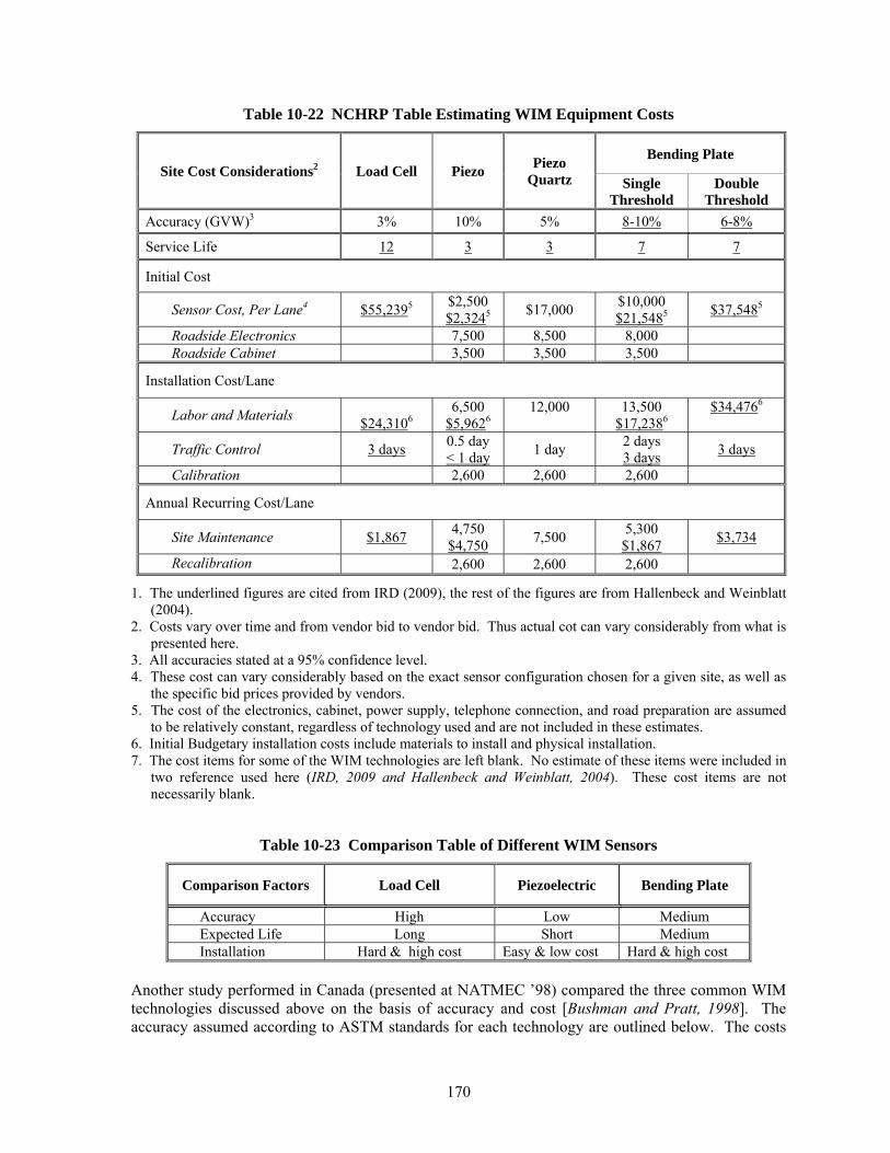
170

Table 10-22 NCHRP Table Estimating WIM Equipment Costs

Site Cost Considerations2 Load Cell Piezo Piezo

Quartz

Bending Plate

Single Threshold

Double Threshold

Accuracy (GVW)3 3% 10% 5% 8-10% 6-8%

Service Life 12 3 3 7 7

Initial Cost

Sensor Cost, Per Lane4 $55,2395 $2,500 $2,3245

$17,000 $10,000 $21,5485

$37,5485

Roadside Electronics 7,500 8,500 8,000 Roadside Cabinet 3,500 3,500 3,500

Installation Cost/Lane

Labor and Materials

$24,3106 6,500

$5,9626 12,000

13,500

$17,2386 $34,4766

Traffic Control 3 days 0.5 day < 1 day

1 day 2 days 3 days

3 days

Calibration 2,600 2,600 2,600

Annual Recurring Cost/Lane

Site Maintenance $1,867 4,750 $4,750

7,500 5,300 $1,867

$3,734

Recalibration 2,600 2,600 2,600

1. The underlined figures are cited from IRD (2009), the rest of the figures are from Hallenbeck and Weinblatt (2004).

2. Costs vary over time and from vendor bid to vendor bid. Thus actual cot can vary considerably from what is presented here.

3. All accuracies stated at a 95% confidence level. 4. These cost can vary considerably based on the exact sensor configuration chosen for a given site, as well as

the specific bid prices provided by vendors. 5. The cost of the electronics, cabinet, power supply, telephone connection, and road preparation are assumed

to be relatively constant, regardless of technology used and are not included in these estimates. 6. Initial Budgetary installation costs include materials to install and physical installation. 7. The cost items for some of the WIM technologies are left blank. No estimate of these items were included in

two reference used here (IRD, 2009 and Hallenbeck and Weinblatt, 2004). These cost items are not necessarily blank.

Table 10-23 Comparison Table of Different WIM Sensors

Comparison Factors Load Cell Piezoelectric Bending Plate

Accuracy High Low Medium Expected Life Long Short Medium Installation Hard & high cost Easy & low cost Hard & high cost

Another study performed in Canada (presented at NATMEC ’98) compared the three common WIM technologies discussed above on the basis of accuracy and cost [Bushman and Pratt, 1998]. The accuracy assumed according to ASTM standards for each technology are outlined below. The costs

171

are the direct costs of the inroad equipment only and do not include related conduit work, system electronics, time delays, etc. The results of the comparison are presented in Table 10-24.

Table 10-24 Comparison Table of Different WIM Sensors

Comparison Factors Piezoelectric Bending Plate Single Load Cell

Accuracy (95% confidence) ± 15 % ± 10 % ± 6 % Expected Life 4 Years 6 Years 12 Years Initial Installation Cost $9,000 $21,500 $48,700

Annual Life Cycle Cost $4,750 $6,400 $8,300

[Bushman & Pratt, 1998]

173

CHAPTER 11. SUMMARY OF RESEARCH METHODOLOGY, FINDINGS AND RECOMMENDATIONS

11.1 Summary of Research Methodology and Findings

This study developed traffic inputs for use with the Guide for the Mechanistic-Empirical Design of New & Rehabilitated Pavement Structures (MEPDG) in North Carolina. The research examined existing NCDOT traffic data resources to identify deficiencies and to recommend candidate locations for future monitoring of traffic data. This study also explored the problem of sampling sparse WIM data to generate estimates of traffic inputs for MEPDG.

11.1.1 Development of Traffic Inputs

To generate MEPDG traffic inputs the WIM volume and weight data are reviewed with respect to completeness and anomalies using a quality control (QC) procedure. The QC procedure involved using an MS Access-based tool that examines each WIM station’s data (44 stations representing about 60 gigabytes of data), identifies the problem data and alerts the user. The user can then replace the data or edit it. The cleaned data are then processed using computer programming to generate traffic factors including VCD, MAF, HDF, ALDF, and number of axles per truck. MEPDG damage-based sensitivity analysis was performed to identify sensitive traffic factors that affect pavement performance measures and those that do not. Performance measures for flexible pavements are rutting, alligator cracking, longitudinal cracking, and the International Roughness Index (IRI). For rigid pavements, only Jointed Plain Concrete Pavement (JPCP) is considered because Continuously Reinforced Concrete Pavement (CRCP) is being phased out from use in the North Carolina road network. The performance measures for JPCP are faulting, percentage of slabs cracked, and the IRI. Structural and materials data were available for LTPP sections only. Representative LTPP sections were used in this sensitivity analysis. To evaluate whether or not the effect of different traffic factors on pavement performance is significant, damage-based sensitivity criteria were developed in cooperation with the North Carolina Department of Transportation (NCDOT). These criteria suggest that an IRI of 14 inches/mile is the limit between being significant and insignificant for both flexible and rigid pavements. Similarly, the limits are 0.1 inch for rutting, 1% of the lane area for alligator cracking, 264 feet/mile for longitudinal cracking, and 0.1 inch for JPCP faulting. Based on the results, flexible pavement performance and rigid pavement performance were found to be insensitive to HDF. Thus, HDF statewide averages may be used for Level 2 and Level 3 design. Similar results are found when comparing the impact on pavement performance of national default values of HDF. This is a valuable finding that simplifies the design process. Similarly, sensitivity analysis showed that rigid pavement performance is insensitive to MAF in NC. For flexible pavements, the predicted fatigue cracking (the most important damage in NC) was found insensitive to MAF for all sites. However, the longitudinal cracking fell beyond the acceptable sensitivity criteria defined by NCDOT. Since the longitudinal cracking model in MEPDG has been found not to be dependable, using engineering judgment, the performance of flexible pavement is assumed to be insensitive to different distributions of MAF experienced in North Carolina. Therefore, the statewide MAF averages are used as input to Levels 2 and 3 pavement designs. The approach simplifies the M-E pavement design process without losing accuracy. Unlike HDF, pavement performance was found to be sensitive to ALDF and VCD. To develop ALDF inputs, multidimensional clustering analysis was proposed. Multidimensional clustering

174

analysis considers similarity of multiple attributes simultaneously and generates ALDF clusters for which their distinctions can be easily explained. In order to decide what axle types and load combinations to include in clustering analysis, the following rules were developed. These rules consider the effect of axle type frequency and damage together:

Rule 1: If the combined effect of damage factors and frequency for a certain axle type-load

combination is less than 1% (normalized damage factor × frequency), this combination can be excluded from ALDF clustering.

Rule 2: If the frequency, i.e., the contribution, of a certain axle type-load combination is less than 1% normalized frequency, this combination can be excluded from ALDF clustering.

When both rules are applied, the 3 – 21 kip load bins (at 1-kip intervals) of the normalized axle load distribution of single axles and 6 – 50 kip load bins (at 2-kip intervals) of the normalized axle load distribution of tandem axles remain. Using the remaining single and tandem axle type-load combinations, multidimensional clustering was carried out. Two-dimensional hierarchical clustering analysis resulted in ALDF clusters of variations in the frequencies of light-weight and heavy-weight single and tandem axles. Post-clustering analysis that incorporates local knowledge of the design road and easy-to-obtain traffic parameters (percent of class 5 and class 9 vehicles derived from 48-hour class counts) found that a strong relation exits between two-dimensional ALDF clusters and the road category: primary arterials, secondary arterials, collectors, and local roadways. These qualitative and quantitative explanatory parameters are summarized in an easy-to-use decision tree that helps the pavement engineer select the proper ALDF input. Damage-based sensitivity analysis also investigated aggregating ALDF clusters based on all 3 sensitive performance parameters for flexible pavements: total rut depth, IRI, and alligator cracking. The results suggest that ALDF clusters cannot be aggregated and should be considered separately. Therefore, it is recommended to include all four ALDF clusters into the final decision tree being developed. The results of the sensitivity analysis also showed that pavement performance was sensitive to VCD. The proposed approach to generate VCD inputs is based on using the site-specific 48-hour vehicle classification counts plus a seasonal factoring procedure that accounts for day-of-week and seasonal variations in truck traffic volume. The proposed approach results in accurate VCD inputs because it incorporates site-specific knowledge of truck traffic. Following TMG recommendations, the seasonal factors are developed for two aggregated vehicle classes: single-unit trucks (SU); and multi-unit trucks (MU). The clustering analysis resulted in four SU and MU factor groups. The traffic parameters (percent of SU trucks and percent of MU trucks) distinguish factor groups and form two decision trees that may be used for selecting the right seasonal factor for converting 48-hour classification counts of SU trucks and MU trucks into annual average volumes. Note that, the 48-hour class counts should be collected on typical weekdays excluding holidays, adverse weather events, and other conditions that cause significant variations in travel. Besides traffic volume adjustment factors (VCD, HDF, and MAF) and ALDF, MEPDG requires some general traffic data to fully characterize the traffic pattern for the design of new or rehabilitated pavement structures. The required traffic data are the same for designing either new or rehabilitated or for either flexible or rigid pavements. These data items describe lateral traffic wander, axle configurations, axle spacing, wheelbase distribution, directional distribution factor, traffic lane distribution, and operational speed. Table 11-1 provides a comprehensive list of MEPDG traffic input requirements and sources of data.

175

Table 11-1 MEPDG Traffic Input Requirements and Sources of Data


(Yes/No) Provider Level 1 Level 2 Level 3

Axle Load Distribution Factor (ALDF) – Flexible Pavement

No TSG based on NC WIM weight data

ALDF files1

ALDF files2 NC User’s Guide

ALDF file3

Axle Load Distribution Factor (ALDF) – Rigid Pavement (JPCP)

ALDF file3

Two Way AADTT Yes TPB


TPB uses the base year AADTT developed by TSG to estimate the future year AADTT

Vehicle Class Distribution (VCD)

Yes TPB


TPB uses the VCD developed by TSG to estimate the VCD for future year

Hourly Distribution Factors (HDF)




Monthly Adjustment Factors (MAF)




Number of Axles per Vehicle Class

Yes TSG based on NC WIM weight data

Appendix 2 (Table A2-5, 6)


Traffic Growth Factor Yes Supplied by TPB/TF Hierarchical levels does not apply

Lateral Traffic Wander Yes

MEPDG Default Values: Mean wheel location = 18 inches from the lane marking Traffic wander standard deviation = 10 inches Design lane width = 12 feet

Axle Configuration Yes

MEPDG Default Values: Average axle width = 8.5 feet Dual tire spacing = 12 inches Tire Pressure = 120 psi

Axle Spacing Yes

Supplied by TSG based on NC WIM weight data tandem axle = 48.9 inches tridem axle = 52.7 inches quad axle = 50.0 inches

Wheelbase Distribution Yes

MEPDG Default Values: Average axle spacing – Short (12 feet), Medium (15 feet), Long (18 feet) Percent of trucks – Short (33%), Medium (33%), Long (34%)

Directional Distribution Factor (DDF)

Yes

MEPDG default values: Class 4, except for local or municipal routes = use 50% Class 4, for local or municipal routes = use 80%-100% Class 5, 6, 7 = use 62% Class 8, 9, 10 = use 55% Class 11, 12, 13 = use 50%

(also shown as Table 4-4)

176

Table 11-2 MEPDG Traffic Input Requirements and Sources of Data (cntd.)


(Yes/No) Supplier

Lane Distribution Factor (LDF)4

Yes

MEPDG default values: Single-lane roadways in one direction = 100% Two-lane roadways in one direction, = 90% Three-lane roadways in one direction = 60% Four-lane roadways in one direction = 45% MEPDG default values is 95%

Operational Speed Yes Supplied by PMU (can be found in Highway Capacity Manual). If local data is not available use MEPDG default values (60 mph)

1. Axle Load Distribution of all 44 WIM sites are delivered electronically in a format of ALDF files. 2. Level 2 ALDF files represent four ALDF clusters, and they are delivered to NCDOT electronically 3. Level 3 ALDF file is the statewide ALDF averages, and it is delivered to NCDOT electronically. 4. PMU Level 3 indicated that national defaults would be used for %Trucks in the design lane

Since traffic data inputs for MEPDG pavement design differ from those currently used in conventional pavement, there is a need to provide clear information on truck traffic forecasting. The study reviewed available truck traffic forecasting methods, NCDOT truck traffic forecasting procedures, truck traffic forecasting options in the M-E pavement design software. Finally, it proposed MEPDG truck traffic forecasting guidelines for NCDOT.

11.1.2 Seasonal Sampling Plan

This part of the research explored the problem of sampling sparse WIM data to generate estimates of traffic inputs for MEPDG. The proposed NC sampling scheme has different frequencies (annual, semiannual, quarterly, and monthly) and different lengths of sampled data (two consecutive weekdays and five consecutive weekdays). The sampling analysis showed that the choice of the proper sampling scheme depends on the seasonal variation of the truck traffic. As expected, where truck traffic is stable (Piedmont region) all sampling schemes are attractive. Where truck traffic is less stable (coastal region) noticeable variations in truck traffic degrade annual-based sampling schemes because annually sampled data cannot sufficiently capture the seasonal variations of truck traffic. The sampling analysis also revealed that knowledge of seasonal variations of truck traffic is necessary to select a proper sampling scheme. It should be noted that besides WIM data, DOTs have other traffic monitoring programs (Continuous Count Programs) that can help them quantify the seasonal variation of truck traffic. Another interesting finding is that increasing the amount of sampled data does not necessarily reduce the error in estimating single and tandem ALDFs. There is relatively little improvement in MSRE% as the sampling scheme changes from five consecutive weekdays per quarter (20 days), to two days per month (24 days), and to five days per month (60 days). This finding results because sampling five consecutive weekdays per quarter can efficiently capture the seasonal variation of truck traffic.

11.1.3 Installation/Abandonment of WIM Sites

Besides providing vehicle weight and volume information for use in pavement design and management, WIM stations provide data for bridge management, overweight vehicle and permit enforcement, and transportation planning. Future applications of WIM stations combined with other technologies will enhance statewide traffic management and freight logistics. Thus, careful attention to WIM station location, replacement and expansion of sites is important. The reliability analysis of seasonal factor groups and ALDF clusters shows at least 22additional WIM sites are needed on some highways to reach the TMG desired levels of precision and confidence. The number of new sites

177

could be adjusted depending on specific NCDOT needs, budget and timetable based on age of sensors in the field. The type of WIM technology to install is also dependent on a tradeoff between many low cost sensors to cover what is needed now versus higher cost sensors that might last longer but reduce the number of locations monitored. Prioritized selections of new WIM locations are made as a result of clustering analysis, ALDF ranking factors, technical installation requirements [TMG, 2001], and NCDOT knowledge of site needs. On the other hand, related seasonal factor group and ALDF reliability analysis shows that TMG levels are exceeded at some factor groups/clusters. Selection of WIM site for abandonment depends upon such factors as: WIM equipment condition, urban/rural location, high/low truck volumes, and the expectation that the traffic pattern at a particular site is established or may change. Seven WIM sites are candidates for abandonment (these WIM sites are presented in Table 10-19). These WIM sites may be prioritized based on their level of depreciation and also the level of truck traffic monitored by them. In general, WIM sites which are depreciated more and monitor fewer number of trucks have higher priority for abandonment.

11.2 Recommendations for Implementation

The outcome of this research project provides the necessary traffic data for the implementation of MEPDG software. Using site-specific traffic data, average values for clustered sites, statewide averages, and default values as recommended in this study (Table 11-1) will allow for pavement designs that more accurately reflect the current traffic loading on roadways in North Carolina. The results of the MEPDG analysis (predicted pavement performance) are only as reliable as the quality of the input data. Thus, the various input factors are critical components to consider in the analysis. The implementation of the recommendations in this study and the use of the MEPDG in general will provide NCDOT with a more advanced means of designing and analyzing pavements. The following paragraphs briefly explain how a user may enter or import the required traffic data for a specific design. A comprehensive traffic data implementation plan is included in MEPDG NC User’s Guide [Kim and Jadoun, 2010]. A summary of the guide is presented in Appendix 6.

11.2.1 Implementation of VCD

To facilitate the process of generating VCD factors for a selected location, an Excel-based VCD Generator & ALDF Cluster Selector tool was developed that can generate VCD factors [Kim and Jadoun, 2010]. The month and day of week seasonal factors, single-unit and multi-unit decision trees are fundamental for the development of the tool. To generate VCD using the tool, the TSG user enters the 48-hour classification counts collected at the design road during typical weekdays (Tuesday-Thursday). The TSG user also specifies whether the counts were collected on Interstate I-95 or not. The tool will automatically generate the base year VCD factors. The base year VCD and AADTT values are sent to TPB/TF to forecast future year AADTT and VCD for the subject highway with and without the improvement. The resulting forecasts are sent to the pavement designer who will manually enter the values in the VCD table in MEPDG.

11.2.2 Implementation of HDF

The statewide HDF averages may be used for North Carolina Levels 2 and 3 designs. Table 4-1 is a summary of state-wide average HDF values that are recommended for use in the MEPDG. Users manually input HDF data in MEPDG software.

11.2.3 Implementation of MAF

The statewide MAF averages may be used for North Carolina Levels 2 and 3 designs. Table 4-2 is a summary of state-wide average MAF values that are recommended for use in the MEPDG. Users

178

may either input MAF data manually or import them directly from MAF file that is delivered to NCDOT.

11.2.4 Traffic Growth Factor

Traffic growth functions and rates will be typically supplied by the TPB/TF. Chapter 5 provides guidelines to choose proper growth rates and functions for single-unit and multi-unit trucks. With MEPDG software the user has the option to manually select the same growth rate and function for all vehicle classes, groups of vehicle classes, or individual classes.

11.2.5 Implementation of General Traffic Input

Here are the other traffic inputs that the user will either manually update or use the national default values:

The manual input data for the number of axles per truck are provided in Table 4-3.

Axle spacing; manually input the data provided in Table 4-4.

Percent trucks in design lane; manually input the data provided in Table 4-4.

Lateral traffic wander; use MEPDG national default values.

Average axle width, tire pressure, and dual tire spacing; use MEPDG national default values.

Wheelbase distribution; use MEPDG national default values.

Percent trucks in design direction; use MEPDG national default values.

Operational speed; use MEPDG national default values.

11.2.6 Implementation of ALDF

The 2-dimensional clustering analysis resulted in four representative ALDF clusters. Four ALDF files are generated that include the average ALDF of WIM sites forming four ALDF clusters. The ALDF files were delivered to NCDOT. A decision tree (Figure 6-18) was also developed that helps the designer select the proper ALDF input given percentage of class 5 and class 9 vehicles at design road as well as the road category: primary highways, secondary highways, collectors or local roads. The ALDF decision tree (Figure 6-18) and class 5% versus class 9% plot (Figure 6-11) are aggregated into the “VCD Generator and ALDF Cluster Selector” tool [Kim and Jadoun, 2010]. The user initially inputs the 48-hour classification counts collected at design road along with roadway category and the tool automatically suggests a representative ALDF cluster. Knowing the ALDF cluster, the user can import the associated ALDF file into MEPDG. There are cases for which the tool fails to suggest any representative ALDF clusters. These are cases that are not represented in the existing WIM data. It is suggested that users refer to Figure 6-11 and use their engineering judgment to select an ALDF cluster that has the closest class 5% and class 9% to those anticipated on the design road.

11.3 Recommendations

11.3.1 Quality Control Procedure

The following recommendations can be implemented to improve upon the quality control procedures.

1. Explore data sampling procedures to reduce the size of databases.

2. Consider quality control as part of a comprehensive process called quality assurance – The quality assurance consists of various quality considerations which are made during data

179

collection and after data summarization and reporting. Some of the quality assurance actions are listed in the following. Develop effective equipment procurement procedures. Establish inspection procedures for newly installed equipments. Schedule periodic maintenance and calibration activities. Develop automated quality control procedure to review and detect corrupt data. Be in contact with the data customer and ask for feedback [Turner, 2007].

3. Assign severity level to quality control rules. Currently, the NCDOT QC database simply

excludes all the data which are rejected based on identified QC rules. In other words, a simple accept/reject decision is made for each rule. It will be more beneficial to assign a severity level to data which are not valid based on QC rules. Suggested severity levels are: High – A high level of severity may happen because of equipment failure. The suggested

action for data with high level of severity would be to exclude the data from further analysis.

Medium – Data with a medium level of severity are outside the acceptance range, however, medium severity is not very significant. The suggested action for data with medium level of severity is to perform more analysis based on local knowledge of traffic and site conditions at the WIM site.

Low – Data with a low level of severity correspond to rules with boundary limits (maximum and minimum limits). It is recommended to investigate such data further based on local knowledge of the WIM site to build more confidence on data quality [Turner, 2007].

4. Plan for long term WIM data storage and analysis. A Microsoft Access database or

spreadsheet program can be used to analyze small datasets, but they are not feasible for analyzing a statewide WIM program. Therefore, the best way to effectively handle the tremendous amount of data generated by a WIM monitoring program is to upload it to a more robust relational database, such as Oracle or Microsoft SQL Server [Nichols et.al, 2004].

11.3.2 Seasonal Factoring Procedure

48-hour classification counts collected at a design location are critical components in selecting the right traffic input for MEPDG. These counts are used for various purposes: to select the proper seasonal factor group using SU and MU factor group decision tree, and to select the proper ALDF cluster using ALDF decision tree. The classification counts are also annualized using seasonal factoring procedure (Chapter 3) and adjusted based on engineering knowledge of TPB/TF staff. The annualized counts are used to generate VCD and AADTT. Considering the important role of the 48-hour counts, NCDOT should supply sufficiently accurate class counts. To produce that accuracy, some data collection recommendations follow:

1. Collect 48-hour class counts on typical days. Exclude holidays, adverse weather events, and

other conditions that cause significant variations in travel. 2. Compare one day’s hourly traffic counts against the second day’s counts to check for any

abnormal patterns in truck traffic. If a significant difference exists between two days’ traffic, then collect additional counts.

3. In most WIM locations, ALDF of single and tandem axles do not vary significantly from month to month. However, there are a few WIM locations for which the ALDF patterns vary

180

in some specific months including July and August. Thus, it is recommended that NCDOT avoid these specific months (July and August) for collecting short duration counts.

As the TMG emphasizes, the seasonal factoring process should be reviewed periodically to ensure that it is performing as intended [TMG, 2001]. For the first few years after initial development, these evaluations should be conducted every year. After that, the seasonal factoring procedure should be reviewed periodically every 3 years. When new WIM data is also available, they should be included in seasonal factoring analysis. New WIM data will help to improve the precision level of seasonal factor groups. Before conducting any analysis using WIM data, it is important to identify observations (WIM sites) that are inconsistent with the remainder of the data (i.e., outliers). These outliers can have a disproportionate effect on the analysis and should be discarded. A graphical presentation of the data set is an easy way to identify outliers. The large number of variables involved (e.g., seasonal factors) rules out the graphical identification of possible outliers. Numerous methods have been suggested for detecting outliers. Principal component analysis is recommended for this purpose because it can be accomplished easily using statistical software including MATLAB.

11.3.3 Seasonal Sampling Plan (Future Research)

This research evaluated the effect of different sampling schemes on the accuracy of the axle load distribution derived from sampled WIM data compared to estimates of ALDFs derived from annual WIM data. Extensive MEPDG simulations need to be conducted to quantify the impact of different sampling on pavement performance (pavement life). In this regards, the MEPDG can be applied to estimate pavement performance until failure under different axle load distributions derived from the proposed sampling schemes. Major pavement distresses (such as fatigue cracking which is the most important damage in NC) could be considered in determining pavement life.

11.3.4 Traffic Forecasts for NCDOT M-E Pavement Design (Future Research)

The most common NCDOT approach for project-level traffic forecasts is utilization of the Traffic Forecasting Utility or TFU (previously called the Trend Program) to develop initial trend line information using linear and / or exponential functions. This tool utilizes ADT and AADT data provided by the Traffic Survey Unit (TSU) and estimates a total traffic growth factor based on available historic years of data. Also, the spreadsheet provides statistical results by analyzing the traffic data from ADT. Some adjustment can be implemented on the existing utility to perform additional analysis using ADT by vehicle class (SUs and MUs). The current utility would need to be adjusted to accommodate historical class counts (VCDs) as well as total traffic counts. The research of HWY 2004-11 describes how truck traffic forecasts may be calculated directly from historic NCDOT truck counts, VTRIS, and WIM data. The findings of the 2004 and this research justify changes to the TFU utility. Other productive future research topics include: the effects of bypass and widening projects on traffic diversion by truck class; truck traffic growth as functions of urban and rural highway classifications including transitions from rural to urban fringe areas; changes in SU and MU truck traffic percentages (of overall traffic) over time; sensitivity of pavement performance to errors in estimated growth rates,

181

and prediction of the growth rate based on roadway characteristics and socio-economic activates. The truck traffic data collected by WIMs and 48-hour counts over years will support the analysis. The expected outcomes may include: different growth patterns for different vehicle classes, the effect of socio-economic activities on growth patterns of different vehicle classes, the sensitivity of the pavement performance to parameters used in the truck traffic growth models (linear or compound), and factors that are associated with traffic growth such as population density and land use.

11.3.5 Installation/Abandonment of WIM Sites

The selection of new WIM locations should be based on the needs of the data collection program and the site characteristics of the roadway sections that meet those needs [TMG 2001]. However, just because a roadway section meets some or all of the above characteristics does not make it a good WIM site. With current technologies, WIM systems only accurately weigh trucks when the equipment is located in a site that meets specific criteria. These criteria include the smoothness of the pavement, access to power and communications, sufficient truck traffic at the site, and etc[TMG 2001]. The recommended number of new sites (22) could be adjusted depending on specific NCDOT needs, and budget. Prioritizing selections of new WIM locations are made as a result of clustering analysis, ALDF ranking factors, technical installation requirements [TMG, 2001], and NCDOT knowledge of site needs. New WIM data will help to improve the precision level of traffic factors derived from seasonal factor groups and ALDF clusters as well as the statewide HDF, statewide MAF, and statewide number of axles per truck. Regardless of the number of WIMs recommended, it is recommended that WIM sites are added in stages, evaluating where they fall in the groups/clusters, before moving on to the next stage and selecting new sites to install. The actual precision levels are evaluated as new WIM sites are installed and the process terminates when the desired level is achieved. The abandonment of WIM sites is recommended to be carried out in stages after ensuring that the discontinuation does not affect the reliability of groups/clusters. For example, the seven candidate WIM sites for abandonments can be discontinued, two locations annually, over a period of three years. The reliability analysis should be repeated every three years to ensure that the desired precision has been maintained. Another important consideration before discontinuation of WIM sites is other use of existing truck information or other reasons that the station is important. NCDOT should ensure that these criteria are met before discontinuing the WIM sites. Finally, a brief discussion on system wide monitoring of truck weights seems relevant. The technique employed in traffic monitoring programs is to have a continuous count component and a coverage count component. The continuous count component is comprised of a limited number of sites where traffic is monitored continuously to provide detailed information on the types of traffic patterns and generate factors for short term counts. The coverage count component is comprised of many locations, enough to define system-wide travel patterns, where short term counts are collected and annualized to provide monitoring of demand on the system. This is done for both volume and vehicle class data types as there are technologies available to collect both continuous and short term counts. This is not the case for truck weights. There is no viable technology to collect truck weights in short

182

term sessions to support a coverage component for this data type. The 2009 AASHTO Guide for Traffic Data Programs Research has shown that these technologies (portable WIMs) are not reliable and that agencies should not use these technologies [AASHTO 2009]. The only methods available to expand the knowledge of the system-wide patterns as related to truck weights are technologies used for the continuous component. The NCSU team recommends that NCDOT manage WIMs so that they meet the continuous component while supporting a process of expanding their knowledge base as there is no coverage component. This requires use of less expensive sensors, reuse of equipment, and makes treatment of pavements impractical. The techniques and guidelines developed in the research supports this approach. The recommendation is to set up a dynamic program, where new WIM sites are added regularly (site selection), adequate data are collected (sampling), sites are discontinued after a short period (site abandonment), while the data needed for MEPDG input are maintained (reliability analysis). The collected data may not be “research quality” data, but they are valuable in expanding the knowledge of system characteristics at a slow and steady pace.

183

REFERENCES

American Society for Testing and Materials. Standard Practice for Classifying Highway Vehicles

from Known Axle Count and Spacing, ASTM E1572-93, 1994. American Association of State Highway Transportation Officials (AASHTO). AASHTO Guidelines

for Traffic Data Programs. ISBN Number: 1-5605-436-7, 2009. Anderberg, M. R. Cluster Analysis for Applications. Academic Press, Inc., New York, New York,

1973, pp.131-145. Applied Research Associate Inc., ERES Consulting Division. Guide for Mechanistic-Empirical

Design of New and Rehabilitated Pavement Structures, Final Report: Part 2. Design Inputs, Chapter 4. Traffic, Champaign, IL., 2004.

Arabie, Ph., J. H. Lawrence, and G. De Soete. Clustering and Classification. World Scientific, 1996. Bushman R., and A. J. Pratt. Weigh In Motion Technology – Economics and Performance, Presented

at NATMEC ’98, Charlotte, North Carolina, 1998. Designing OLAP Cubes, http://www.databaseanswers.org/designing_olap_cubes.htm, Accessed July

1, 2009 Elkins L., and C. Higgins. Development of Truck Axle Spectra from Oregon Weigh-in-Motion Data

for Use in Pavement Design and Analysis, Research Unit, Oregon Department of Transportation, 2008.

FHWA Vehicle Types, Office of Highway Policy Information, FHWA, US Department of

Transportation, http://www.fhwa.dot.gov/policy/ohpi/vehclass.htm, Accessed July 4, 2009. Hallenbeck, M. Long Term Pavement Performance Traffic Monitoring Protocol. FHWA,

Washington, D.C., 1998. Hallenbeck, M. E., and S. G. Kim. Final Technical Report for Task A: Truck Loads and Flows,

Washington State Transportation Center (TRAC), WA-RD 320.3, 1993. Hallenbeck, M. E., M. Rice, B. Smith, C. Cornell-Martinez, and J. Wilkinson. Vehicle Volume

Distributions by Classification. Washington, DC: Long-Term Pavement Performance Division, Federal Highway Administration, 1997.

Hallenbeck M. and H. Weinblatt. Equipment for Collecting Traffic Load Data, NCHRP Report 509,

2004. Hong, F., J. A. Prozzi, and A. Leung. Sampling Schemes for Weigh-in-Motion Traffic Data

Collection, Transportation Research Record, No. 2043, 2008, pp. 38-44. Highway Performance Monitoring System (HPMS). Field Manual for the Continuing Analytical and

Statistical Database, Office of Highway Policy Information. FHWA, US Department of Transportation, http://www.fhwa.dot.gov/policy/ohpi/hpms/index.cfm, 2005.

184

International Road Dynamics Inc. (IRD), WIM Technologies Comparison, Revision A, 2009. Jadoun, F. M., F. Sayyady, Y. R. Kim, and J. R. Stone. Damage-Based Clustering Analysis to Guide

the Development of MEPDG Axle Load Factors for North Carolina, Submitted to 90th TRB Annual Meeting, Washington, D.C., 2011.

Jolliffe, I. T. Principal Component Analysis, 2nd edition, Springer, 2002. Kim, J. R., L. Titus-Glover, M. I. Darter, and R. K. Kumapley. Axle Load Distribution

Characterization For Mechanistic Pavement Design, Transportation Research Record, No. 1629, 1998, pp. 13–23.

Clyde L. E., and N. Souny-Slitine. Final Research Findings on Traffic-Load Forecasting Using

Weigh-In-Motion Data, Research Report 987-7. Center for Transportation Research, The University of Texas at Austin, 1998.

Li, S., Y. Jiang, and K. Zhu. Truck Traffic Characteristics for Mechanistic-Empirical Flexible

Pavement Design: Evidences, Sensitivities, and Implications. In CD-ROM, 86th TRB Annual Meeting, Washington, D.C., 2007.

Liu R., X. Chen, J. Li, L. Guo, and J. Yu. Evaluate Innovative Sensors and Techniques for Measuring

Traffic Loads, Final Report, TxDOT 0-4509, 2005. LTPP Information Management System (IMS) Quality Control Checks, FHWA, US Department of

Transportation, http://www.fhwa.dot.gov/PAVEMENT/pub_details.cfm?id=284, Updated October 2005.

LTPP Traffic QC Software, Volume 1: Users Guide. Software version 1.6., FHWA, US Department of Transportation. November 2001.

Lu, Q., and J. T. Harvey. Characterization of Truck Traffic in California for Mechanistic-Empirical

Design. Transportation Research Record, No. 1945, 2006, pp. 61–72. Lu Q., Y. Zhang, and J. T. Harvey. Estimation of Truck Traffic Inputs for M-E Pavement Design In

California. In CD-ROM, 84th TRB Annual Meeting, Washington, D.C., 2009. Kim, Y. R., and F. Jadoun, MEPDG NC User’s Guide, Research Project No. HWY-2007-07,

Prepared for North Carolina Department of Transportation, 2010. Mastin, Neil, Weigh-in-Motion Database and Processor Project Documentation, Department of Civil,

Construction, and Environmental Engineering, North Carolina State University, Master’s Thesis, 2007.

Mojena, R. Hierarchical Grouping Methods and Stopping Rules: An Evaluation. The Computer

Journal, No. 20 (4), 1977, pp. 359–363. National Cooperative Highway Research Program (NCHRP). Development of the 2002 Guide for the

Design of New and Rehabilitated Pavement Structures: Determination of Traffic Information and Data for Pavement Structural Design and Evaluation, Final Report, NCHRP 1-37A, Transportation Research Board of the National Academies, Washington D.C., 2004.

185

National Cooperative Highway Research Program (NCHRP) Traffic Data Collection, Analysis, and Forecasting for Mechanistic Pavement Design. Technical Report 538, Project 1-39, Transportation Research Board of the National Academies, Washington, D.C., 2005.

National Cooperative Highway Research Program (NCHRP). AASHTO Guide for Design of

Pavement Structures. Washington D.C., 1993. Nicholas, A. P., and D. Bullock. Quality Control Procedures for Weigh-in-Motion Data.

FHWA/IN/JTRP-2004/12, Indiana Department of Transportation and FHWA, US Department of Transportation, 2004.

Papagiannakis (a), A., T., M. Bracher, and N. C. Jackson. Utilizing Clustering Techniques in

Estimating Traffic Data Input for Pavement Design. Journal of Transportation Engineering, No. 132, 2006, pp. 872–879.

Papagiannakis (b), A.T., M. Bracher, J. Li, and N. Jackson. Optimization of Traffic Data Collection

for Specific Pavement Design Applications, FHWA-HRT-05-079, 2006. Prozzi, J. A., and F. Hong. Hierarchical Axle Load Data for Mechanistic-Empirical Design. In

Proceedings CD-ROM, 84th TRB Annual Meeting, Washington, D.C., 2005. Qu T., C. E. Lee, and L. Huang. Traffic-Load Forecasting Using Weigh-in-Motion Data, Research

Report 987-6, Center for Transportation Research, University of Texas at Austin, 1997. Ramachandran, A., K. L. Taylor, J. R. Stone, and S. Sajjadi. NCDOT Quality Control Methods for

Weigh in Motion Data. In Proceedings CD-ROM, 89th TRB Annual Meeting, Washington, DC, 2010.

Sarasota-Manatee Metropolitan Planning Organization, FHWA Vehicle Types, www.sarasota-

manateempo.org/Figures/figure1.pdf, Accessed June 15, 2009. Sayyady, F., J. R. Stone, K. L. Taylor, F. M. Jadoun, and Y. R. Kim. Using Clustering Analysis to

Characterize MEPDG Traffic Data in North Carolina, In Proceedings CD-ROM, 89th TRB Annual Meeting, Washington, D.C., 2010.

Sayyady, F., J. R. Stone, G. F. List, F. M. Jadoun, Y. R. Kim, and S. S. Sajjadi. Multidimensional

Clustering to Characterize Axle Load Distribution for MEPDG in North Carolina. Will appear in Transportation Research Record, Washington, D.C, 2011.

Shawn T. Quality Control Procedures for Archived Operations Traffic Data, Synthesis of Practice and

Recommendations, Texas Transportation Institute, The Texas A&M University System, Prepared for Office of Highway Policy Information, Federal Highway Administration, 2007.

Sherif, I., H-C. Shin, B. Sridhar, and Z. Zhang. Characterization and Development of Truck Axle

Load Spectra for Future Implementation of New Pavement Design Practices in Louisiana, In CD-ROM, 89th TRB Annual Meeting, Washington, D.C., 2010.

SQL Server Analysis Services Tutorial, http://technet.microsoft.com/en-us/library/ms170208.aspx,

Accessed June 20, 2009

186

Stone J.R., Han Y., Ramkumar R., North Carolina Forecasts for Truck Traffic, NCDOT Report HWY 2004-11, 2006.

Swan, D., J., R. Tardif, J. J. Hajek, and D. K. Hein. Development of Regional Traffic Data for the

Mechanistic-Empirical Pavement Design Guide. Transportation Research Record, No. 2049, 2008, pp. 54–62.

Szary, P. J. and A. Maher. Implementation of Weigh-in-Motion (WIM) Systems, Final Report,

FHWA-NJ-2009-00, 2009. Timm, D. H., J. M. Bower, and R. E. Turochy. Effect of Load Spectra on Mechanistic-Empirical

Flexible Pavement Design. Transportation Research Record: Journal of the Transportation Research Board, No. 1947, 2006, pp. 146–154.

Traffic Monitoring Guide, FHWA, US Department of Transportation, May 2001. Traffic Monitoring Guide, Section 4, Vehicle Classification Monitoring, FHWA, Department of

Transportation, May 2001. Traffic Monitoring Guide, Section 5, Truck Weight Monitoring, FHWA, Department of

Transportation, May 2001. Tran, N. H., and K. D. Hall. Development and Influence of Statewide Axle Load Spectra on Flexible

Pavement Performance. Transportation Research Record, No. 2037, 2007, pp. 106–114. Vehicle Travel Information System (VTRIS), Office of Highway Policy Information. FHWA, US

Department of Transportation, http://www.fhwa.dot.gov/ohim/ohimvtis.cfm, Accessed May 8, 2009.

Wang Y., D. E. Hancher, and K. Mahboub. Axle Load Distribution for Mechanistic–Empirical

Pavement Design. Journal of Transportation Engineering, Vol. 133, No. 8, 2007, pp. 469–479. Wang K. User’s Guide of Database Support for AHTD MEPDG, Department of Civil Engineering,

University of Arkansas, 2009. Washington State Department of Transportation Pavement Guide, http://training.ce.washington.edu/wsdot/Modules/04_design_parameters/wim.htm Weinblatt, H. Using seasonal and day-of-week factoring to improve estimates of truck vehicle miles

traveled. Transportation Research Record, 1522, 1996, pp. 1-8.

187

APPENDIX 1

ACRONYMS

Acronym

Meaning

AADTT Annual Average Daily Truck Traffic AADT Annual Average Daily Traffic ADT Average Daily Traffic ALDF Axle Load Distribution Factors APT Axles per Truck AASHTO American Association of State Highway and Transportation Officials BY Base Year CRCP Continuously Reinforced Concrete Pavement DOW Day of Week DDF Directional Distribution Factor FHWA Federal Highway Administration FC Functional Class FY Future Year HDF Hourly Distribution Factors HPMS Highway Performance Monitoring System IRD International Road Dynamics IRI International Roughness Index JPCP Jointed Plain Concrete Pavement (JPCP) LDF Lane Distribution Factor LTPP Long Term Pavement Performance MAF Monthly Adjustment Factors MADTT Monthly Average Day-of-week Truck Traffic MEPDG Mechanistic Empirical Pavement Design Guide MU Multi-Unit Trucks (Vehicle Classes 8-13) NCSU North Carolina State University PC Principal Component PCA Principal Component Analysis PDU Pavement Design Unit SU Single-Unit Trucks (Vehicle Classes 4-7) TFU Traffic Forecasting Utility TPB Transportation Planning Branch TPB/TF Transportation Planning Branch/Traffic Forecast TMG Traffic Monitoring Guide TSG Traffic Survey Group VCD Vehicle Class Distribution VTRIS Vehicle Travel Information System WIM Weigh-in-Motion

189

APPENDIX 2

LEVEL 1 TRAFFIC DATA FOR THE 44 WIM SITES

Table A2-1 Annual Average Daily Truck Traffic for the 44 WM Sites

SHRP ID

Site ID

Route Name

Location Lanes County Nearest

City/Town AADTT


371030 502 US 17 0.4 Miles South of US 158 2S, 2N. Pasquotank Elizabeth

City 1175

371645 504 US 74 1.9 Miles West of SR 1001 2W, 2E. Columbus Whiteville 1649 371805 508 US 64 0.7 Miles West of US 15-501 2W, 2E. Chatham Pittsboro 839 372824 509 US 421 1.9 Miles South of US 64 2S, 2N. Chatham Siler City 1968 372819 511 US 220 1.6 Miles North of NC 62 2S, 2N. Guilford Greensboro 2969 371817 512 US 311 0.6 Miles East of SR 2698 2S. Forsyth Salem - 375826 515 I-77 0.5 Miles North of SR 1345 (Mp 98) 2S, 2N. Surry Mount Airy 7092 372825 516 SR 1138 0.7 Miles East of NC 49 2W, 2E. Mecklenburg Charlotte 604 375037 519 I-40 1.6 Miles West of SR 2838 (Mp 55) 2W. Buncombe Oteen - 371801 520 I-40 1.3 Miles West of SR 2740 2W, 2E. Buncombe Swannanoa 6093 371024 521 NC 107 0.3 Miles North of SR 1001 1N, 1S Jackson Cullowhee 367 371803 522 US 74-441 0.2 Miles East of SR 1391 2W, 2E. Jackson Whittier 1155 371814 523 US 23-441 0.2 Miles South of SR 1504 2S, 2N. Macon Franklin 1039 371992 525 US 421 0.8 Miles North of US 64 2S, 2N. Chatham Siler City 1945 377302 529 US 264 0.3 Miles West of NC 33 2W, 2E. Pitt Greenville 1467 370900 530 US 1 0.1 Miles South of SR 1423 2S, 2N. Lee Sanford 1736 370200 531 US 52 0.4 Miles North of US 64 (Mp 92) 2S, 2N. Davidson Lexington 3039 370800 532 SR 1245 0.1 Miles North of SR 1209 1N, 1S Onslow Jacksonville - 372101 533 US 64 0.5 Miles East of SR 1304 1E, 1W Clay Hayesville 354 371901 534 US 64 0.4 Miles East of US 19/129 2W, 2E. Cherokee Murphy 760 371902 535 US 74 0.3 Miles West of SR 1390 2W, 2E. Cherokee Andrews 507 374301 536 I-40 1.0 Miles West of US 19-23-74 Conn 2W, 2E. Haywood Clyde 8142 377401 537 I-26 0.5 Miles East of US 74 (MP 67) 2W, 2E. Polk Columbus 4428 372202 538 I-85 0.3 Miles East of NC 161 (MP 8) 2S, 2N. Cleveland Kings 11583 375902 539 I-77 0.1 Miles South of I-485 (Mp 2) 3N, 3S Mecklenburg Charlotte 9611 377701 541 I-95 1.0 Miles South of NC 130 (Mp 1) 2S, 2N. Robeson McDonald 8027 377001 542 I-40 0.3 Miles West of NC 210 (Mp 408) 2W, 2E. Pender Rocky Point 1710 379201 543 I-85 0.2 Miles East of US 1 (Mp 233) 2S, 2N. Warren Wise 5370 375903 546 NC 24 0.2 Miles East of US 21 2W, 2E. Mecklenburg Charlotte 1922 373501 547 US 321 0.1 Miles South of NC 279 3S, 3N. Gaston Dallas 4716 374701 548 US 264 0.1 Miles East of SR 1168 1W, 1E. Hyde Scranton 4705.014 377002 549 US 421 0.2 Miles South of NC 210 2S, 2N. Pender Currie 535 378201 551 US 74 0.1 Miles East of NC 79 2W, 2E. Scotland Laurinburg 2401 370301 552 US 74 0.1 Miles West of SR 1740 2W, 2E. Anson Lilesville 2146 377501 553 US 220 0.1 Miles North of SR 1247 2S, 2N. Randolph Asheboro 2652 377803 554 US 220 0.5 Miles South of SR 2150 2S, 2N. Rockingham Madison 2630 374002 555 NC 68 0.5 Miles North of Bryan Blvd 2S, 2N. Guilford Greensboro 2393 371003 556 I-240 0.5 Miles East of US 70 (Mp 8) 2E, 3W. Buncombe Asheville 1643 374801 557 I-40 0.3 Miles West of US 21 (Mp 151) 2W, 2E. Iredell Statesville 8907 371701 558 US 321 1.0 Miles North of I-40 (At US 70) 2S, 2N. Catawba Hickory 2835 371101 559 I-40 0.3 Miles West of SR 1744 (Mp 109) 2W, 2E. Burke Valdese 6158 375601 560 I-26 0.1 Miles West of US 19 (Mp 3) 2W, 2E. Madison Mars Hill 1141

190

Table A2-1 Annual Average Daily Truck Traffic for the 44 WM Sites (continued)

SHRP ID

Site ID

Route Name

Location Lanes Nearest

City/Town Nearest

City/Town AADTT


371028 501 US 17 0.7 Miles North of SR 1231

2N. South Mills South Mills 942

371402 540 2S. South Mills South Mills 373011 503

I-95 0.5 Miles South of SR 1745 2N. Rocky Mount Rocky Mount

7300 376302 527 2S. Rocky Mount Rocky Mount 373102 545

NC 147 0.4 Miles North of SR 1940 2S. Durham Durham

2219 373816 507 2N. Durham Durham 371006 506

I-40 0.8 Miles East of NC 54 2E. Raleigh Raleigh

6959 379102 544 2W. Raleigh Raleigh 375827 510

US 29 1.8 Miles North of US 158 2S. Reidsville Reidsville

2032 377802 526 2N. Reidsville Reidsville

191

Table A2-2 Vehicle Class Distribution for the 44 WM Sites

WIM ID VC 4 VC 5 VC 6 VC 7 VC 8 VC 9 VC 10 VC 11 VC 12 VC 13

501/540 2.59 36.27 6.51 0.43 3.70 49.06 0.76 0.60 0.04 0.04

502 2.22 38.85 8.88 0.45 3.65 42.72 0.84 0.47 0.04 0.06503/527 3.53 12.46 4.54 0.04 3.18 74.51 0.50 0.65 0.54 0.07

504 3.71 20.03 9.19 0.30 3.63 59.86 0.78 1.48 0.90 0.13506/544 7.40 25.77 8.90 0.29 10.22 45.07 1.16 0.80 0.29 0.10507/545 7.76 41.90 10.13 0.37 7.05 30.95 0.73 0.75 0.25 0.10

508 6.01 32.77 5.76 0.32 5.64 47.39 0.82 0.45 0.63 0.20509 3.49 17.73 8.83 0.31 4.90 61.34 1.02 1.92 0.16 0.31

510/526 4.13 11.93 3.86 0.11 9.98 63.33 0.40 5.42 0.80 0.04511 6.15 25.89 6.13 0.41 4.46 54.05 1.25 1.27 0.36 0.04515 3.87 10.07 4.73 0.10 2.33 73.03 0.37 3.83 1.62 0.04516 28.51 47.13 9.05 0.78 7.04 6.92 0.46 0.03 0.01 0.06520 4.19 16.78 6.10 0.50 3.24 65.92 0.46 2.11 0.63 0.07521 3.82 55.12 11.98 0.87 22.78 4.95 0.47 0.00 0.00 0.01522 5.56 38.73 13.69 1.13 17.40 22.32 0.88 0.11 0.06 0.11523 5.43 47.47 5.71 0.44 3.91 36.58 0.29 0.08 0.02 0.08525 4.69 18.20 5.50 0.24 4.36 64.13 1.35 1.35 0.12 0.06529 4.02 23.53 12.76 1.03 5.59 50.61 0.87 0.93 0.52 0.13530 4.23 25.09 11.05 0.51 4.75 51.42 1.64 0.28 0.12 0.91531 5.37 17.87 4.30 0.13 4.38 61.35 0.37 4.36 1.83 0.04533 4.80 51.16 15.13 2.31 10.64 14.86 1.08 0.00 0.01 0.01534 4.50 51.24 9.62 0.83 10.63 22.34 0.63 0.01 0.00 0.21535 4.13 42.71 9.65 0.73 8.34 32.19 2.14 0.01 0.01 0.09536 2.59 5.99 2.60 0.09 6.44 76.46 0.56 4.19 1.03 0.06537 3.16 11.12 3.27 0.09 6.94 71.62 0.74 2.49 0.50 0.07538 4.23 9.56 3.85 0.09 6.38 69.44 0.32 4.57 1.51 0.04539 5.94 16.24 7.10 0.41 10.56 55.41 0.50 2.57 1.23 0.05541 4.04 7.63 3.43 0.14 8.82 73.78 0.63 0.74 0.54 0.26542 7.71 32.42 6.71 0.22 5.48 44.82 1.00 1.04 0.39 0.21543 4.96 6.67 2.01 0.12 6.12 74.61 0.41 4.10 0.97 0.03546 9.49 48.01 10.00 1.51 5.95 19.07 0.82 3.61 1.47 0.07547 5.97 23.83 6.40 0.47 4.94 55.77 0.33 1.43 0.83 0.03548 5.92 41.43 11.62 0.16 4.24 34.87 1.41 0.01 0.00 0.35549 0.92 26.87 14.77 0.49 4.31 50.15 1.42 0.70 0.20 0.16551 3.58 16.29 14.10 0.85 3.63 58.20 0.76 1.80 0.67 0.12552 5.39 19.17 7.70 0.59 3.85 58.84 1.32 2.03 1.06 0.04553 4.47 19.14 5.84 0.32 5.85 61.53 1.49 0.99 0.34 0.03554 5.05 16.26 6.87 1.45 4.59 59.15 0.52 4.75 1.34 0.02555 6.24 30.13 10.54 0.86 4.23 47.13 0.58 0.15 0.12 0.02556 6.63 53.00 9.23 0.77 3.76 25.89 0.43 0.10 0.16 0.04557 4.83 18.66 4.83 0.18 5.86 62.45 0.41 2.21 0.52 0.06558 6.63 24.16 6.77 0.36 8.59 52.58 0.47 0.14 0.28 0.03559 4.83 16.49 4.47 0.10 4.44 66.38 0.40 2.14 0.65 0.11

560 7.33 19.46 5.33 0.20 5.54 60.76 0.47 0.55 0.29 0.06

192

Table A2-3 Hourly Distribution Factors for the 44 WM Sites

WIM ID Midnight

1:00 am

2:00 am

3:00 am

4:00 am

5:00 am

6:00 am

7:00 am

8:00 am

9:00 am

10:00 am

11:00 am

Noon1:00 pm

2:00 pm

3:00 pm

4:00 pm

5:00 pm

6:00 pm

7:00 pm

8:00 pm

9:00 pm

10:00 pm

11:00 pm

501/540 1.22 1.16 0.87 1.29 1.69 3.49 4.90 5.04 6.15 6.86 7.24 7.06 6.91 6.92 6.83 6.62 5.85 5.27 4.08 3.06 2.30 2.02 1.76 1.44

502 1.03 0.98 1.22 1.52 2.58 4.13 5.32 6.28 7.00 7.18 7.23 7.05 7.72 7.04 6.62 6.02 5.70 4.10 3.12 2.24 2.00 1.51 1.30 1.11

503/527 2.56 2.25 2.11 2.06 2.25 2.59 3.27 3.83 4.46 5.14 5.51 5.60 5.65 5.64 5.66 5.72 5.67 5.57 5.05 4.55 4.25 3.88 3.63 3.09

504 1.29 1.28 1.65 2.05 2.53 3.67 4.69 5.13 5.67 6.29 6.81 6.81 6.94 6.42 6.22 5.97 5.41 4.99 4.05 3.27 2.90 2.49 1.90 1.55

506/544 1.46 1.41 1.43 1.54 2.19 3.09 4.95 5.58 6.02 6.73 7.04 6.88 6.58 6.48 6.33 6.02 5.33 4.62 4.23 3.34 2.65 2.24 2.08 1.80

507/545 1.34 1.00 1.05 1.42 1.68 2.66 5.03 6.46 6.99 7.04 7.13 6.88 6.54 6.37 6.55 6.63 5.79 5.23 4.01 2.77 2.22 2.02 1.72 1.48

508 1.33 1.18 1.63 2.28 3.46 4.35 5.15 6.39 6.74 6.90 6.78 6.49 6.60 6.50 6.38 6.10 5.09 4.17 3.32 2.75 2.00 1.88 1.39 1.15

509 1.97 1.58 1.95 2.52 3.50 4.37 4.92 5.81 6.70 6.80 6.74 6.51 6.47 6.14 5.77 5.08 4.39 3.85 3.18 2.78 2.61 2.35 2.13 1.88

510/526 2.54 2.25 2.13 2.29 2.96 3.69 4.49 4.59 4.92 5.55 5.74 5.76 5.49 5.40 5.53 5.31 5.32 4.94 4.24 4.07 3.75 3.31 3.02 2.73

511 1.44 1.40 1.59 2.21 3.25 5.21 5.66 6.20 6.49 6.45 6.48 6.35 6.30 6.20 6.00 5.52 5.06 4.15 3.28 2.76 2.39 2.10 1.84 1.67

515 2.39 2.19 2.35 2.47 2.77 3.07 3.59 4.16 4.72 5.18 5.31 5.49 5.56 5.64 5.67 5.58 5.41 5.04 4.89 4.54 4.14 3.82 3.26 2.76

516 1.27 1.09 0.86 0.81 0.95 2.09 2.90 4.00 5.71 6.84 7.54 7.13 6.80 7.28 6.96 6.72 6.93 6.13 4.99 4.09 3.28 2.22 1.89 1.53

520 2.19 2.16 2.17 2.45 2.76 3.47 4.35 5.10 5.55 5.88 5.98 5.97 5.92 5.90 5.75 5.49 5.08 4.49 4.02 3.75 3.45 3.07 2.69 2.35

521 0.56 0.37 0.26 0.27 0.36 1.38 3.39 6.46 7.34 7.32 7.17 7.27 7.37 7.65 7.50 8.46 7.59 6.41 4.49 3.09 2.04 1.64 0.98 0.63

522 0.99 0.91 0.96 1.12 1.52 2.18 4.08 5.02 6.86 7.64 8.10 8.05 7.52 7.45 7.21 6.74 5.97 5.16 3.73 2.70 1.98 1.64 1.37 1.10

523 1.07 0.98 1.14 1.52 2.07 3.57 5.44 6.39 7.12 7.24 7.35 7.23 7.25 7.05 6.85 6.37 5.71 4.16 3.13 2.47 2.00 1.72 1.28 0.91

525 1.85 1.55 1.89 2.53 3.69 4.49 5.08 6.05 6.80 6.65 6.67 6.48 6.41 6.07 5.74 5.05 4.35 3.85 3.21 2.84 2.60 2.29 2.04 1.82

529 0.88 0.83 1.07 1.53 2.68 4.21 6.08 7.28 7.49 7.55 7.23 6.90 7.08 6.90 6.61 5.92 5.04 3.65 2.75 2.41 2.03 1.65 1.29 0.93

530 1.23 1.45 1.97 2.73 3.79 5.26 5.86 6.91 7.33 7.50 7.32 7.07 6.75 6.41 5.74 5.06 4.26 3.24 2.53 2.02 1.62 1.46 1.33 1.15

531 2.20 1.93 2.09 2.69 3.41 4.38 5.06 5.91 6.49 6.45 6.27 5.99 5.87 5.78 5.41 4.94 4.39 3.79 3.30 2.93 2.82 2.95 2.54 2.41

533 0.53 0.55 0.55 0.61 0.56 1.13 3.61 6.44 7.02 7.52 8.60 7.86 7.54 7.72 8.02 8.03 6.60 5.57 3.54 2.43 1.99 1.58 1.23 0.78

534 0.79 0.75 0.70 1.19 1.48 2.22 3.14 5.02 6.56 7.36 7.72 7.74 7.66 7.79 7.62 7.36 6.61 5.29 3.91 2.85 2.32 1.76 1.25 0.91

535 1.01 0.87 1.29 1.70 1.87 2.54 4.66 5.66 6.00 6.95 7.07 7.22 6.90 7.10 6.99 6.67 6.12 5.39 4.22 2.98 2.29 1.87 1.47 1.16

536 3.20 2.83 2.61 2.57 2.66 2.80 2.90 3.30 3.74 4.27 4.85 5.11 5.26 5.27 5.40 5.50 5.46 5.37 5.24 4.91 4.68 4.37 4.08 3.62

537 2.35 2.10 2.00 2.12 2.53 2.89 3.53 4.16 4.73 5.40 5.85 6.17 6.07 5.96 5.82 5.69 5.40 5.18 4.63 4.10 3.74 3.57 3.22 2.79

193

Table A2-3 Hourly Distribution Factors for the 44 WM Sites (continued)

WIM ID Midnight

1:00 am

2:00 am

3:00 am

4:00 am

5:00 am

6:00 am

7:00 am

8:00 am

9:00 am

10:00 am

11:00 am

Noon1:00 pm

2:00 pm

3:00 pm

4:00 pm

5:00 pm

6:00 pm

7:00 pm

8:00 pm

9:00 pm

10:00 pm

11:00 pm

538 3.08 2.75 2.70 2.69 3.01 3.31 3.65 3.84 4.36 5.01 5.37 5.42 5.39 5.37 5.37 5.31 5.12 4.76 4.56 4.32 3.94 3.74 3.63 3.29

539 2.01 1.94 2.17 2.54 3.39 4.27 4.19 5.09 6.06 6.40 6.40 6.13 6.01 5.93 5.53 5.03 4.53 4.40 3.78 3.34 3.09 2.89 2.58 2.28

541 2.68 2.35 2.29 2.28 2.55 2.78 3.18 3.63 4.28 5.03 5.63 5.88 5.86 5.71 5.60 5.52 5.38 5.24 4.93 4.59 4.23 3.92 3.40 3.05

542 1.32 1.28 1.66 2.19 2.98 4.51 5.37 6.34 6.99 6.90 7.20 6.25 6.23 6.34 6.32 5.80 5.13 4.14 3.10 2.63 2.23 1.65 2.20 1.25

543 3.27 2.90 2.75 2.95 3.21 3.49 3.60 3.80 4.03 4.39 4.89 5.16 5.22 5.06 4.99 4.98 5.01 4.83 4.57 4.36 4.25 4.29 4.22 3.80

546 1.17 1.08 1.28 1.86 2.89 5.52 6.63 7.26 7.43 7.33 7.07 6.84 6.80 6.64 6.15 5.63 4.55 3.40 2.54 2.15 1.64 1.50 1.41 1.22

547 1.73 1.70 1.85 2.10 3.04 4.45 5.30 5.92 6.26 6.45 6.36 6.20 6.12 6.12 5.88 5.57 4.85 4.22 3.48 3.09 2.77 2.58 2.13 1.84

548 0.42 0.43 0.55 1.22 2.63 4.78 6.19 7.79 8.02 7.58 7.53 7.18 7.39 7.15 7.74 6.76 5.43 3.77 2.44 1.75 1.16 0.89 0.62 0.60

549 0.82 0.93 1.37 2.11 3.03 5.28 6.41 6.79 7.36 7.53 6.95 6.96 6.47 6.92 6.77 5.88 5.29 3.70 2.68 2.18 1.54 1.06 1.08 0.89

551 1.73 2.00 2.29 2.84 3.54 4.35 4.90 5.45 5.95 6.35 6.84 6.62 6.38 5.95 5.52 5.11 4.49 4.05 3.34 3.11 2.97 2.45 1.99 1.78

552 1.89 1.95 2.39 3.21 3.84 4.71 4.90 5.49 6.05 6.51 6.68 6.53 6.30 6.06 5.67 5.06 4.35 3.61 3.12 2.71 2.55 2.60 2.08 1.75

553 1.41 1.32 1.84 2.61 3.78 4.81 5.49 6.20 6.71 6.91 6.79 6.64 6.50 6.15 5.54 4.94 4.44 3.79 3.25 2.73 2.37 2.18 1.96 1.64

554 1.90 1.79 1.95 2.40 3.22 4.36 4.98 5.48 6.13 6.31 6.28 6.21 6.30 6.41 6.08 5.33 4.75 4.04 3.43 3.04 2.75 2.58 2.22 2.05

555 1.38 1.35 1.36 1.64 2.57 4.57 5.69 6.45 6.66 6.64 6.56 6.42 6.59 6.62 6.47 6.01 5.28 3.98 3.34 2.69 2.31 2.08 1.77 1.56

556 0.91 0.69 0.63 0.83 1.16 1.68 3.72 6.01 6.89 7.54 7.54 7.54 7.39 7.45 7.43 7.04 6.31 5.47 4.12 2.92 2.20 1.82 1.56 1.16

557 1.81 1.68 1.79 2.27 2.88 3.74 4.54 5.26 5.85 6.13 6.24 6.26 6.30 6.23 6.05 5.64 5.13 4.53 3.81 3.46 3.13 2.80 2.42 2.04

558 1.80 1.88 2.24 2.61 3.34 4.31 5.49 6.54 6.72 6.99 6.70 6.43 6.80 6.76 6.08 5.22 4.23 3.39 2.67 2.26 2.14 1.96 1.85 1.60

559 2.07 1.89 2.05 2.23 2.70 3.47 4.34 4.98 5.57 6.02 6.10 6.08 6.09 6.07 5.86 5.59 5.14 4.54 4.02 3.67 3.42 3.13 2.66 2.31

560 1.79 1.58 1.66 2.14 2.88 3.55 4.18 5.10 5.88 6.43 6.36 6.22 6.04 5.97 5.72 5.41 5.17 4.69 4.33 3.71 3.45 3.08 2.63 2.03

194

Table A2-4 Monthly Adjustment Factors for the 44 WM Sites

WIM ID January February March April May June July August September October November December

501/540 0.9 1.0 1.0 1.1 1.0 1.2 1.1 0.9 0.9 1.0 1.0 0.9

502 0.9 0.8 1.0 1.1 1.1 1.2 1.2 0.9 0.9 1.0 1.0 1.0

503/527 1.0 1.0 1.0 1.1 1.1 1.1 1.0 1.0 0.9 1.0 1.0 1.0

504 0.9 1.0 1.0 1.0 1.0 1.1 1.0 1.0 1.0 1.0 0.9 0.9

506/544 0.9 1.0 1.0 1.0 1.0 1.1 1.0 1.1 1.0 1.0 1.0 0.9

507/545 0.9 0.9 1.0 1.0 1.0 1.0 0.9 1.1 1.1 1.2 1.1 0.9

508 0.9 0.9 1.0 1.0 1.0 1.0 1.0 1.0 1.0 1.1 1.0 0.9

509 0.9 0.9 1.0 1.0 1.1 1.1 1.0 1.0 1.0 1.0 1.0 0.9

510/526 0.9 1.0 1.0 1.0 1.0 1.0 0.9 1.0 1.0 1.1 1.0 0.9

511 1.0 1.0 1.0 1.0 1.0 1.0 1.0 1.0 1.0 1.1 1.0 0.9

515 0.9 0.9 1.0 1.0 1.0 1.1 1.0 1.0 1.0 1.1 1.0 0.9

516 0.8 0.9 1.0 1.2 1.0 1.0 1.0 1.1 1.1 1.0 0.9 1.0

520 0.9 0.9 1.0 1.0 1.0 1.1 1.0 1.1 1.0 1.1 1.0 0.9

521 0.8 0.8 0.9 1.1 1.1 1.2 1.2 1.1 1.0 1.0 1.0 0.8

522 0.8 0.8 0.9 1.0 1.0 1.1 1.2 1.2 1.1 1.2 1.0 0.8

523 0.9 0.9 1.0 1.1 1.1 1.1 1.1 1.0 1.0 1.1 1.0 0.9

525 0.8 0.9 1.0 1.0 1.1 1.1 1.0 1.1 1.0 1.1 1.0 0.9

529 1.0 1.0 1.0 1.1 1.0 1.1 0.9 1.0 1.0 1.1 1.0 1.0

530 0.9 0.9 1.1 1.1 1.0 1.0 1.0 0.9 1.1 0.9 0.9 1.1

531 1.0 1.0 1.0 1.0 1.0 1.0 1.0 1.0 1.0 1.0 1.0 0.9

533 0.7 0.8 1.0 1.2 1.1 1.2 1.3 1.2 1.2 1.2 0.7 0.5

534 0.9 0.9 0.9 1.0 1.1 1.1 1.1 1.1 1.0 1.1 1.0 0.8

535 0.8 1.0 1.1 1.1 1.1 1.1 0.9 0.8 1.1 1.0 1.0 1.1

536 1.0 1.0 1.0 1.0 1.0 1.0 1.0 1.0 1.1 1.1 1.0 0.9

537 0.9 1.0 1.0 1.0 1.0 1.0 1.0 1.0 1.0 1.1 1.0 0.9

538 0.9 1.0 1.1 1.1 1.0 1.0 1.0 1.0 1.0 1.0 1.0 0.9

539 0.9 1.0 1.1 1.0 1.0 1.0 1.0 1.0 1.0 1.0 1.0 0.9

541 1.0 1.0 1.0 1.0 1.0 1.0 0.9 1.0 1.0 1.1 1.0 1.0

542 0.9 0.9 1.0 1.0 1.1 1.1 1.0 1.1 0.9 1.0 0.9 1.0

543 1.0 1.0 1.0 1.0 1.0 1.0 1.0 1.0 1.0 1.1 1.0 0.9

546 0.9 1.0 1.1 1.0 1.1 1.0 1.0 1.1 1.0 0.9 0.9 1.0

547 0.9 1.0 1.1 1.0 1.0 1.0 1.0 1.1 1.0 1.1 1.0 0.9

548 0.8 1.0 0.9 1.0 0.9 1.1 0.9 1.0 1.1 1.1 1.2 0.9

549 0.9 1.0 1.0 1.1 1.0 1.1 1.0 1.0 1.0 0.9 0.8 1.1

551 1.0 1.0 1.0 1.0 1.0 1.0 1.0 1.0 1.0 1.1 1.0 0.9

552 1.0 1.0 1.0 1.0 1.0 1.0 1.0 1.0 1.0 1.0 1.0 0.9

553 1.0 1.0 1.0 1.0 1.0 1.0 1.0 1.0 1.0 1.0 1.0 0.9

554 0.9 0.9 1.1 1.1 1.0 1.1 1.0 1.0 1.0 1.1 1.0 0.9

555 1.0 1.0 1.0 1.1 1.0 1.0 1.0 1.1 1.0 1.1 0.9 0.9

556 0.9 0.9 1.1 1.0 1.0 1.1 1.0 1.0 1.0 1.1 1.0 0.9

557 0.9 0.9 1.1 1.0 1.0 1.1 1.0 1.1 1.0 1.0 1.0 0.9

558 0.9 1.0 1.0 1.0 1.0 1.1 1.0 1.1 1.0 1.0 0.9 0.9

559 0.9 0.9 1.1 1.0 1.0 1.0 1.0 1.1 1.0 1.1 1.0 0.9

560 1.0 1.0 1.1 1.1 1.1 1.2 1.1 1.3 0.9 0.8 0.6 0.8

195

Table A2-5 Number of Axles for Single and Tandem Axle Types for the 44 WM Sites

Single Tandem

Class 4 Class 5 Class 6 Class 7 Class 8 Class 9 Class 10 Class 11 Class 12 Class 13 Class 4 Class 5 Class 6 Class 7 Class 8 Class 9 Class 10 Class 11 Class 12 Class 13

501/540 1.23 2.00 1.25 1.02 2.39 1.22 1.03 5.00 4.00 1.09 0.77 0.00 0.86 0.33 0.61 1.89 1.35 0.00 1.00 0.58

502 1.19 2.00 1.26 1.05 2.44 1.24 1.02 5.00 4.00 1.53 0.81 0.00 0.87 0.17 0.56 1.88 1.18 0.00 1.00 0.50

503/527 1.70 2.00 1.57 1.27 2.52 1.27 1.00 5.00 4.00 2.23 0.30 0.00 0.68 0.33 0.48 1.87 1.29 0.00 1.00 1.94

504 1.92 2.00 1.17 1.10 2.42 1.23 1.00 5.00 4.00 1.98 0.08 0.00 0.91 0.11 0.58 1.88 1.45 0.00 1.00 2.33

506/544 1.84 2.00 1.13 1.13 2.62 1.15 1.01 5.00 4.00 1.13 0.16 0.00 0.93 0.16 0.39 1.92 1.11 0.00 1.00 0.48

507/545 1.66 2.00 1.26 1.09 2.51 1.15 1.01 5.00 4.00 1.26 0.34 0.00 0.85 0.19 0.49 1.92 1.23 0.00 1.00 0.69

508 1.86 2.00 1.01 1.13 2.37 1.22 1.00 5.00 4.00 1.11 0.14 0.00 0.99 0.10 0.63 1.89 1.40 0.00 1.00 2.79

509 1.89 2.00 1.12 1.05 2.33 1.17 1.00 5.00 4.00 2.31 0.11 0.00 0.94 0.07 0.67 1.91 1.09 0.00 1.00 1.94

510/526 1.74 2.00 1.01 1.25 2.60 1.12 1.03 5.00 4.00 1.21 0.26 0.00 0.99 0.09 0.40 1.94 1.41 0.00 1.00 0.56

511 1.73 2.00 1.00 1.05 2.23 1.22 1.00 5.00 4.00 1.88 0.27 0.00 1.00 0.09 0.77 1.89 0.99 0.00 1.00 1.90

515 1.76 2.00 1.01 1.23 2.34 1.25 1.01 5.00 4.00 2.13 0.24 0.00 0.99 0.22 0.66 1.88 1.28 0.00 1.00 2.40

516 1.95 2.00 1.01 1.02 2.72 1.16 2.20 5.00 4.00 2.50 0.05 0.00 0.99 0.07 0.28 1.80 0.94 0.00 1.00 1.40

520 1.86 2.00 1.01 1.04 2.25 1.18 1.00 5.00 4.00 1.38 0.14 0.00 0.99 0.14 0.75 1.91 1.34 0.00 1.00 1.70

521 1.98 2.00 1.00 1.00 2.89 1.14 1.00 0.00 0.00 1.25 0.02 0.00 1.00 0.28 0.11 1.90 1.45 0.00 0.00 0.50

522 1.80 2.00 1.08 1.01 2.88 1.17 1.01 5.00 4.00 1.05 0.20 0.00 0.95 0.37 0.12 1.91 1.35 0.00 1.00 0.68

523 1.91 2.00 1.02 1.05 2.47 1.19 1.00 4.99 4.00 1.00 0.09 0.00 0.98 0.09 0.52 1.90 1.33 0.01 1.00 1.00

525 1.81 2.00 1.00 1.05 2.25 1.18 1.00 5.00 4.00 1.68 0.19 0.00 1.00 0.05 0.75 1.91 1.03 0.00 1.00 2.60

529 1.91 2.00 1.18 1.02 2.44 1.11 1.01 5.00 4.00 2.06 0.09 0.00 0.91 0.05 0.56 1.94 1.27 0.00 1.00 2.21

530 1.92 2.00 1.12 1.08 2.38 1.22 1.00 5.00 4.00 1.10 0.08 0.00 0.94 0.15 0.62 1.89 0.82 0.00 1.00 0.98

531 1.81 2.00 1.01 1.17 2.20 1.13 1.02 5.00 3.99 2.03 0.19 0.00 0.99 0.39 0.80 1.94 1.23 0.00 1.00 2.47

533 1.92 2.00 1.06 1.00 2.82 1.13 1.01 4.50 4.00 1.09 0.08 0.00 0.96 0.32 0.18 1.93 1.49 0.25 1.00 1.27

534 1.84 2.00 1.16 1.03 2.83 1.22 1.06 5.00 4.00 1.08 0.16 0.00 0.89 0.30 0.17 1.86 1.38 0.00 1.00 0.84

535 1.86 2.00 1.12 1.08 2.91 1.15 1.06 4.87 4.00 1.31 0.14 0.00 0.93 0.43 0.12 1.91 1.41 0.07 1.00 0.50

536 1.74 2.00 1.23 1.20 2.77 1.19 1.11 5.00 4.00 1.30 0.26 0.00 0.86 0.29 0.31 1.90 1.20 0.00 1.00 0.44

196

Table A2-5 Number of Axles for Single and Tandem Axle Types for the 44 WM Sites (continued)

Single Tandem


537 1.81 2.00 1.05 1.38 2.62 1.16 1.01 5.00 4.00 1.19 0.19 0.00 0.97 0.12 0.38 1.92 1.31 0.00 1.00 0.67

538 1.81 2.00 1.05 1.38 2.62 1.16 1.01 5.00 4.00 1.19 0.19 0.00 0.97 0.12 0.38 1.92 1.31 0.00 1.00 0.67

539 1.80 2.00 1.21 1.04 2.45 1.19 1.01 5.00 4.00 1.32 0.20 0.00 0.89 0.07 0.55 1.91 1.28 0.00 1.00 0.79

541 1.60 2.00 1.32 1.74 2.85 1.23 1.14 5.00 4.00 1.52 0.40 0.00 0.81 0.48 0.25 1.88 1.24 0.00 1.00 0.55

542 1.85 2.00 1.45 1.06 2.42 1.20 1.00 5.00 4.00 1.12 0.15 0.00 0.75 0.16 0.58 1.90 1.34 0.00 1.00 1.15

543 1.64 2.00 1.24 1.69 2.68 1.21 1.08 5.00 3.99 1.33 0.36 0.00 0.87 0.26 0.36 1.89 1.28 0.00 1.00 0.65

546 1.92 2.00 1.00 1.01 2.25 1.14 1.00 5.00 4.00 1.60 0.08 0.00 1.00 0.06 0.75 1.92 1.23 0.00 1.00 1.27

547 1.86 2.00 1.01 1.04 2.19 1.12 1.01 5.00 4.00 2.22 0.14 0.00 0.99 0.06 0.81 1.94 1.28 0.00 1.00 2.39

548 1.87 2.00 1.25 1.11 2.63 1.07 1.00 5.00 0.00 0.00 0.13 0.00 0.87 0.21 0.37 1.96 1.52 0.00 0.00 0.00

549 1.70 2.00 1.15 1.01 2.37 1.22 1.00 5.00 3.98 1.20 0.30 0.00 0.91 0.08 0.63 1.89 1.40 0.00 0.99 2.90

551 1.90 2.00 1.10 1.25 2.39 1.18 1.00 5.00 4.00 2.00 0.10 0.00 0.95 0.32 0.61 1.91 1.18 0.00 1.00 2.08

552 1.80 2.00 1.00 1.06 2.27 1.17 1.00 5.00 4.00 1.52 0.20 0.00 1.00 0.15 0.73 1.92 1.07 0.00 1.00 2.67

553 1.80 2.00 1.01 1.07 2.16 1.23 1.00 5.00 4.00 2.19 0.20 0.00 0.99 0.08 0.84 1.89 0.97 0.00 1.00 2.41

554 1.88 2.00 1.00 1.01 2.16 1.15 1.00 5.00 4.00 1.71 0.12 0.00 1.00 0.24 0.84 1.92 1.14 0.00 1.00 2.65

555 1.88 2.00 1.00 1.01 2.16 1.15 1.00 5.00 4.00 1.71 0.12 0.00 1.00 0.24 0.84 1.92 1.14 0.00 1.00 2.65

556 1.87 2.00 1.01 1.03 2.41 1.13 1.00 5.00 4.00 1.00 0.13 0.00 0.99 0.20 0.59 1.93 1.65 0.00 1.00 1.67

557 1.83 2.00 1.01 1.14 2.18 1.18 1.01 5.00 4.00 2.14 0.17 0.00 0.99 0.09 0.82 1.91 1.21 0.00 1.00 2.41

558 1.84 2.00 1.01 1.05 2.10 1.11 1.00 5.00 4.00 2.04 0.16 0.00 0.99 0.06 0.90 1.95 1.19 0.00 1.00 2.48

559 1.90 2.00 1.01 1.16 2.21 1.20 1.00 5.00 4.00 2.39 0.10 0.00 0.99 0.14 0.79 1.90 1.32 0.00 1.00 2.27

560 1.87 2.00 1.03 1.08 2.39 1.24 1.00 5.00 4.00 1.57 0.13 0.00 0.97 0.09 0.61 1.88 1.34 0.00 1.00 1.71

197

Table A2-6 Number of Axles for Tridem and Quad Axle Types for the 44 WM Sites

Tridem Quad


501/540 0.00 0.00 0.00 0.67 0.00 0.00 0.61 0.00 0.00 1.50 0.00 0.00 0.00 0.00 0.00 0.00 0.04 0.00 0.00 0.02

502 0.00 0.00 0.00 0.83 0.00 0.00 0.37 0.00 0.00 0.99 0.00 0.00 0.00 0.00 0.00 0.00 0.25 0.00 0.00 0.25

503/527 0.00 0.00 0.00 0.59 0.00 0.00 0.70 0.00 0.00 0.00 0.00 0.00 0.00 0.00 0.00 0.00 0.00 0.00 0.00 0.06

504 0.00 0.00 0.00 0.88 0.00 0.00 0.48 0.00 0.00 0.00 0.00 0.00 0.00 0.00 0.00 0.00 0.04 0.00 0.00 0.00

506/544 0.00 0.00 0.00 0.81 0.00 0.00 0.43 0.00 0.00 1.50 0.00 0.00 0.00 0.00 0.00 0.00 0.27 0.00 0.00 0.03

507/545 0.00 0.00 0.00 0.80 0.00 0.00 0.46 0.00 0.00 1.14 0.00 0.00 0.02 0.00 0.00 0.00 0.17 0.00 0.00 0.11

508 0.00 0.00 0.00 0.86 0.00 0.00 0.51 0.00 0.00 0.00 0.00 0.00 0.00 0.00 0.00 0.00 0.04 0.00 0.00 0.05

509 0.00 0.00 0.00 0.92 0.00 0.00 0.52 0.00 0.00 0.00 0.00 0.00 0.00 0.00 0.00 0.00 0.20 0.00 0.00 0.06

510/526 0.00 0.00 0.00 0.84 0.00 0.00 0.48 0.00 0.00 1.11 0.00 0.00 0.00 0.00 0.00 0.00 0.10 0.00 0.00 0.25

511 0.00 0.00 0.00 0.90 0.00 0.00 0.50 0.00 0.00 0.00 0.00 0.00 0.00 0.00 0.00 0.00 0.41 0.00 0.00 0.32

515 0.00 0.00 0.00 0.75 0.00 0.00 0.60 0.00 0.00 0.00 0.00 0.00 0.00 0.00 0.00 0.00 0.08 0.00 0.00 0.00

516 0.00 0.00 0.00 0.93 0.00 0.02 0.58 0.00 0.00 0.20 0.00 0.00 0.00 0.00 0.00 0.04 0.01 0.00 0.00 0.25

520 0.00 0.00 0.00 0.86 0.00 0.00 0.65 0.00 0.00 0.03 0.00 0.00 0.00 0.00 0.00 0.00 0.01 0.00 0.00 0.51

521 0.00 0.00 0.00 0.72 0.00 0.00 0.54 0.00 0.00 0.50 0.00 0.00 0.00 0.00 0.00 0.00 0.00 0.00 0.00 0.75

522 0.00 0.00 0.00 0.62 0.00 0.00 0.51 0.00 0.00 0.83 0.00 0.00 0.00 0.00 0.00 0.00 0.14 0.00 0.00 0.46

523 0.00 0.00 0.00 0.90 0.00 0.00 0.65 0.00 0.00 0.00 0.00 0.00 0.00 0.00 0.00 0.00 0.01 0.00 0.00 1.00

525 0.00 0.00 0.00 0.94 0.00 0.00 0.51 0.00 0.00 0.00 0.00 0.00 0.00 0.00 0.00 0.00 0.32 0.00 0.00 0.00

529 0.00 0.00 0.00 0.95 0.00 0.00 0.62 0.00 0.00 0.00 0.00 0.00 0.00 0.00 0.00 0.00 0.05 0.00 0.00 0.00

530 0.00 0.00 0.00 0.85 0.00 0.00 0.34 0.00 0.00 0.11 0.00 0.00 0.00 0.00 0.00 0.00 0.42 0.00 0.00 0.86

531 0.00 0.00 0.00 0.57 0.00 0.00 0.54 0.00 0.00 0.00 0.00 0.00 0.00 0.00 0.00 0.00 0.13 0.00 0.00 0.00

533 0.00 0.00 0.00 0.68 0.00 0.00 0.30 0.00 0.00 0.55 0.00 0.00 0.00 0.00 0.00 0.00 0.21 0.00 0.00 0.18

534 0.00 0.00 0.00 0.69 0.00 0.00 0.48 0.00 0.00 1.16 0.00 0.00 0.00 0.00 0.00 0.00 0.10 0.00 0.00 0.01

535 0.00 0.00 0.00 0.56 0.00 0.00 0.31 0.00 0.00 1.16 0.00 0.00 0.00 0.00 0.00 0.00 0.24 0.00 0.00 0.13

536 0.00 0.00 0.00 0.68 0.00 0.00 0.59 0.00 0.00 1.37 0.00 0.00 0.00 0.00 0.00 0.00 0.13 0.00 0.00 0.09

198

Table A2-6 Number of Axles for Tridem and Quad Axle Types for the 44 WM Sites (continued)

Tridem Quad


537 0.00 0.00 0.00 0.78 0.00 0.00 0.66 0.00 0.00 0.94 0.00 0.00 0.00 0.00 0.00 0.00 0.02 0.00 0.00 0.37

538 0.00 0.00 0.00 0.78 0.00 0.00 0.66 0.00 0.00 0.94 0.00 0.00 0.00 0.00 0.00 0.00 0.02 0.00 0.00 0.37

539 0.00 0.00 0.00 0.92 0.00 0.00 0.56 0.00 0.00 1.22 0.00 0.00 0.00 0.00 0.00 0.00 0.14 0.00 0.00 0.05

541 0.00 0.00 0.00 0.33 0.00 0.00 0.60 0.00 0.00 0.97 0.00 0.00 0.00 0.00 0.00 0.00 0.06 0.00 0.00 0.22

542 0.00 0.00 0.00 0.84 0.00 0.00 0.59 0.00 0.00 0.34 0.00 0.00 0.01 0.00 0.00 0.00 0.04 0.00 0.00 0.56

543 0.00 0.00 0.00 0.59 0.00 0.00 0.64 0.00 0.00 1.10 0.00 0.00 0.00 0.00 0.00 0.00 0.04 0.00 0.00 0.18

546 0.00 0.00 0.00 0.94 0.00 0.00 0.65 0.00 0.00 0.82 0.00 0.00 0.00 0.00 0.00 0.00 0.11 0.00 0.00 0.05

547 0.00 0.00 0.00 0.93 0.00 0.00 0.36 0.00 0.00 0.00 0.00 0.00 0.00 0.00 0.00 0.00 0.34 0.00 0.00 0.00

548 0.00 0.00 0.00 0.79 0.00 0.00 0.42 0.00 0.00 0.00 0.00 0.00 0.00 0.00 0.00 0.00 0.03 0.00 0.00 0.00

549 0.00 0.00 0.00 0.92 0.00 0.00 0.58 0.00 0.01 0.00 0.00 0.00 0.01 0.00 0.00 0.00 0.01 0.00 0.00 0.00

551 0.00 0.00 0.00 0.67 0.00 0.00 0.57 0.00 0.00 0.00 0.00 0.00 0.00 0.00 0.00 0.00 0.12 0.00 0.00 0.08

552 0.00 0.00 0.00 0.84 0.00 0.00 0.46 0.00 0.00 0.00 0.00 0.00 0.00 0.00 0.00 0.00 0.36 0.00 0.00 0.03

553 0.00 0.00 0.00 0.90 0.00 0.00 0.52 0.00 0.00 0.00 0.00 0.00 0.00 0.00 0.00 0.00 0.41 0.00 0.00 0.00

554 0.00 0.00 0.00 0.76 0.00 0.00 0.41 0.00 0.00 0.00 0.00 0.00 0.00 0.00 0.00 0.00 0.31 0.00 0.00 0.00

555 0.00 0.00 0.00 0.76 0.00 0.00 0.41 0.00 0.00 0.00 0.00 0.00 0.00 0.00 0.00 0.00 0.31 0.00 0.00 0.00

556 0.00 0.00 0.00 0.79 0.00 0.00 0.32 0.00 0.00 0.00 0.00 0.00 0.00 0.00 0.00 0.00 0.02 0.00 0.00 0.67

557 0.00 0.00 0.00 0.87 0.00 0.00 0.58 0.00 0.00 0.00 0.00 0.00 0.00 0.00 0.00 0.00 0.17 0.00 0.00 0.01

558 0.00 0.00 0.00 0.92 0.00 0.00 0.26 0.00 0.00 0.00 0.00 0.00 0.00 0.00 0.00 0.00 0.48 0.00 0.00 0.00

559 0.00 0.00 0.00 0.82 0.00 0.00 0.64 0.00 0.00 0.00 0.00 0.00 0.00 0.00 0.00 0.00 0.02 0.00 0.00 0.01

560 0.00 0.00 0.00 0.89 0.00 0.00 0.65 0.00 0.00 0.00 0.00 0.00 0.00 0.00 0.00 0.00 0.01 0.00 0.00 0.43

199

APPENDIX 3

EXAMPLE TRAFFIC FORECASTING PROBLEM

Traditionally TPB Traffic Forecasters have produced future year AADT estimates for the project highway with and without improvement. They usually do not annualize vehicle classification counts collected in the base year. They express the base year truck class counts as percentages of base year AADT, specifically, percent single unit trucks (Duals) and percent truck tractor single trailer trucks (TTSTs). And they usually carry forward the base year truck percentages of AADT from the base year to the future year without a forecast adjustment unless there is significant reason to do so, like a new truck distribution hub or manufacturing center. Furthermore, the truck counts are not annualized, while the total traffic AADT is (by definition). This inconsistency is overcome when the TPB forecasters assume constant percent Duals and TTSTs from base to future year. The AADT forecasts and the constant base year to future year truck percentages have traditionally been used in North Carolina pavement design. However, the MEPDG pavement design procedures require forecast values for truck distributions which are truck class percentages based on total truck traffic, not total vehicle AADT traffic (as discussed under “Terminology” in the Executive Summary). MEPDG requires either individual truck class forecasts or aggregate truck class forecasts. This appendix uses aggregate classes for single unit trucks (SUs), which are equivalent to truck classes 4-7 and multiunit trucks (MUs) equivalent to remaining classes 8-13. This appendix discusses forecasts for the truck classes and the growth function to be used in MEPDG pavement design for North Carolina. Furthermore, the appendix develops consistency between annualized traffic forecasts and annualized truck volumes that are used to generate forecasts of truck vehicle class distributions (VCD). Elizabethtown Bypass, R-522, Bladen County

As an example of the traffic forecasting procedures required for MEPDG consider the Elizabethtown Bypass in Bladen County (Figures A3-1 and A3-2). The following steps use the Elizabethtown R-522 case to illustrate the guidelines of Chapter 5 to develop the MEPDG inputs for pavement design.

Figure A3-1 Elizabethtown Bypass and Business Routes NC 87 (Source Google Maps)

200

Figure A3-2 Elizabethtown Bypass and Business Routes NC 87 (Source NCDOT, 2008 AADT) 1. Discard vehicle classes 1 to 3. For pavement design light weight vehicle classes 1-3 will be ignored.

However, light weight vehicles make up the majority of vehicle volumes and will continue to be part of the usual NCDOT forecasts for highway planning and design.

2. Consider two aggregated truck classes. Data analysis for traffic forecasts can be simplified by

considering two aggregate truck classes: SU trucks (classes 4-7) and MU trucks (classes 8-13). SU and MU terminology is equivalent to Duals and TTSTs, respectively. Although the SU and MU percentages are still required for the traffic forecast, the more detailed VCD is required for pavement design. VCD are percentages of annualized truck traffic (AADTT), not percentages based on counts (not seasonally factored) as used for DUALs and TTSTs currently. It is recommended that the data used to generate SU (Duals) and MU (TTST) for the traffic forecast be based on the annualized truck volumes that are used to generate VCD. This will provide consistent data for both processes and will support transference of analyses performed for the traffic forecast to the pavement design data and vice versa.

3. Determine the base year traffic without improvement (no-build). Since we do not have the data for

NC 87 west of the bypass, we are going to assume it is the sum of the business and bypass volumes. For a forecast like this, the TSG will collect a class count on the existing route where the bypass will meet the business route. We are using the class data as provided. The TSG needs to deliver annualized data to the TPB/TF staff member when this process is implemented. We are using 2008 as the base year and forecasting to 2035 as this is the typical method used in the forecasting process.

Table A3-1 2008 Data - Treated as Annualized Data for Demonstration Purposes

Route Station 1* 2 3 4 5 6 7 8 9 10 11 12 13 AADTT (sum 4-13)

AADT (sum 1-13)

Bypass VC0818 1 2012 639 51 143 25 2 59 340 11 1 0 0 632 3284 Business VC0822 4 2601 855 49 133 60 3 15 13 3 0 0 1 277 3737

* Numbers 1 to 13 corresponds to 13 vehicle classes of FHWA vehicle classification scheme (see Table 3 of Executive Summary).

201

This combined data set would be representative of the counts collected on the existing facility and is used for the base year below. The combined data would represent the base year traffic without improvement.

Table A3-2 Base Year Traffic without Improvement (No-Build)

Route 1 2 3 4 5 6 7 8 9 10 11 12 13 AADTT AADT NC 87 5 4613 1494 100 276 85 5 74 353 14 1 0 1 909 7021

SU MU

Truck Percentages

100 276 85 57021

6.6% 74 353 14 1 0 1

70216.3%

4 5 6 7 8 9 10 11 12 13

Vehicle Class Distribution 100909

0.11 0.30 0.09 0.01 0.08 0.39 0.02 0.00 0.00 0.00

Note: This data must be provided in the report for a vehicle classification count collected by TSG. 4. Determine the base year traffic with improvement (build). Regarding traffic diverted to the bypass

from the original business NC 87, Table A3-3 shows that in 2008 90% of the MU trucks, which are primarily on long haul through trips, took the NC 87 Bypass while 10% of the MU trucks stayed on NC 87 Business. On the other hand, 44% of the SU trucks took the bypass and 56% use the original business route through town. This is reasonable since SU trips are shorter and often serve local destinations. Such information regarding percentage trips by SU and MU class diverted to a proposed bypass can support refined estimates of traffic forecasts for pavement design purposes. Traffic monitoring of class data should be conducted for small, medium and large sized communities to support a database of bypass diversions for use in the traffic forecasts for similar facilities. The diversion rates included in Table A3-3 are taken from a similar facility bypassing a similar town.

Table A3-3 Diversion Rates

Route Passenger Vehicles SU MU Bypass 0.39 0.44 0.9 Business 0.61 0.56 0.1

Table A3-4 Calculated NC 87 Bypass Estimate

Route 1 2 3 4 5 6 7 8 9 10 11 12 13 AADTT AADT

NC 87 Bypass 0.39 52 1799 583 44 121 37 2 67 318 13 1 0 1 604 2988

SU MU

Truck Percentages 44 12 37 2

29886.8%

67 318 13 1 0 12988

13.4%

4 5 6 7 8 9 10 11 12 13

Vehicle Class Distribution 44604

0.07 0.20 0.06 0.00 0.11 0.53 0.02 0.00 0.00 0.00

202

5. Generate the traffic forecasts required by the MEPDG. After the network traffic estimates have been developed for the base year 2008 build scenario for the bypass, traffic forecasts may be made. The TPB/TF needs to generate the following items required for the mechanistic-empirical pavement design. Base Year AADTT – for total trucks as needed for input into the software Base Year VCD – as needed for input into the software; forecasters can perform their analysis

using aggregated classes (SU and MU) but must disaggregate to the ten VCD classes as a last step to provide to the pavement designers

Truck Growth Rate(s) – This statistic can be developed using AADT growth (the current practice) aggregated classes (SU and MU), or individual truck classes (the 10 VCD classes)

Truck Growth Function – Should be identical to AADT function if AADT growth is used 6. Generate future year traffic with improvement. We consider four growth scenarios to demonstrate the

different options and the calculations required to use those options to generate the above mentioned items (base year AADTT, base year VCD, truck growth rate and functions):

203

Scenario 1 - Match AADT Growth The TPB/TF forecaster calculates AADT linear growth rates in the area on NC 87 and estimates the average rate to be 2.6% per year. Assume that the investigation of future conditions indicates that the future growth in this area will be similar to historic patterns. The forecaster uses the historic rate to estimate traffic projections. Future truck percentages are the same as base year. Traffic Forecast Estimates:

Year AADT 2008 round 2988 3000 2035 round 2988 1 2035 2008 0.026 5100

Type Truck % SU round 6.8% 7% MU round 13.4% 13%

Pavement Design Estimates:

2008 AADTT 600

Class 4 5 6 7 8 9 10 11 12 13

2008 VCD 0.07 0.20 0.06 0.00 0.11 0.53 0.02 0.00 0.00 0.00

Growth Rate 2.6%

Growth Function Linear

204

Scenario 2 - Adjust Future Year Truck Percentages The TPB/TF forecaster calculates AADT linear growth rates in the area on NC 87 and estimates the average rate to be 2.6% per year. Assume that the investigation of future conditions indicates that the future growth will deviate significantly from historic patterns. Significant residential development has begun in the area. A number of developers have stated residential developments on the bypass alignment and one includes a shopping center. Future growth is estimated to be 5% compounded annually. Traffic Forecast Estimates:

Year AADT 2008 round 2988 3000 2035 round 2988 1 0.05 11200

The high truck percentages in the base year imply the high mobility (diversion to the bypass) the improvement has for trucks whereas many passenger vehicles are still attracted to Elizabethtown. The type of development expected to occur has few trucks and the high volumes in the forecast year will be more passenger vehicle oriented. The forecaster decides to adjust the truck percentages to reflect this trend. The SU trucks will be less impacted by the bypass than MU trucks which make few trips to residential development.

Base Year Adjustment Amount Forecasted Truck% SU 7% -3% 4% MU 13% -6% 7%

Pavement Design Estimates: The adjustment of truck percentages means that the truck growth rates do not match AADT. Additionally, the difference in the adjustment means that the SU growth rate is different from the MU growth rate to obtain this future distribution of trucks. Base year and future year truck volumes for SU and MU must be calculated to use as the basis for calculating individual growth rates.

2008 2035 Linear Growth Rates

SU 7% 3000 210 4% 11200 448 448 210 210⁄

2035 2008100 4.20%

MU 390 784 3.74%

2008 AADTT 600

Class 4 5 6 7 8 9 10 11 12 13 2008 VCD 0.07 0.20 0.06 0.00 0.11 0.53 0.02 0.00 0.00 0.00 Class Group SU MU Growth Rate 4.2% 3.8% Growth Function Linear Linear

205

Scenario 3 - Calculation Based Truck Growth Rates The forecaster calculates AADT linear growth rates in the area on NC 87 and estimates the average rate to be 2.6% per year. Investigation of plans for the area indicates that the future growth in this area will be similar to historic patterns. The forecaster uses the historic rate to estimate AADT projections. The forecaster finds current and historic vehicle classification data on the NC 87 corridor. They perform a trend analysis on historic truck growth patterns for SU and MU truck groups. The data shows that linear growth rates are 2.5% for SU and 2.0% for MU. Plans for the area indicate that truck growth will be similar to historic patterns. In this scenario, the forecaster has an estimate of individual growth rates for AADT, SU, and MU. Although they have base year truck percentages, they don't know what impact the different growth rates will have on future truck percentages. The forecaster must calculate future AADT, SU, and MU volumes to calculate the future truck percentages needed in the traffic forecast. Traffic Forecast Estimates:

Year AADT 2008 round 2988 3000 2035 round 2988 1 2035 2008 0.026 5100

Type Linear

Growth Rate 2008 2035 Truck %

SU 2.50% 44 121 37 2204

204 1 2035 2008 2.5% =342

3425100

100 7%

MU 2.00% 67 318 13 10 1 400

400 1 2035 2008 2.0% 616 6165100

100 12%

Pavement Design Estimates:

2008 AADTT 600

Class 4 5 6 7 8 9 10 11 12 13

2008 VCD 0.07 0.20 0.06 0.00 0.11 0.53 0.02 0.00 0.00 0.00

Class Group SU MU

Growth Rate 2.5% 2.1%

Growth Function Linear Linear

206

Scenario 4 - Adjustment of Individual Classes The forecaster calculates AADT linear growth rates in the area on NC 87 and estimates the average rate to be 2.6% per year. Investigation of plans for the area uncovers a development in progress for a FedEx distribution center to be built at the east end of the bypass. A traffic impact analysis was performed as part of the permitting process providing detailed analysis of traffic with the facility including an estimate of the number of trips on the bypass for the specific vehicle types used by FedEx. These are:

Type Trips Class 5 800 Class 8 150 Class 11 50 Total 1000

Based on the study and the anticipation that related development for the area will increase the forecaster estimates AADT will grow at 3.3% per year linearly. The forecaster estimates growth in background truck volumes will be the same. The forecaster must add the FedEx truck trips to the future background trucks to generate both future truck percentages for the forecast and the individual growth rates for each vehicle class. Truck Analysis by Class: Class 4 5 6 7 8 9 10 11 12 13 2008 Trucks 44 121 37 2 67 318 13 1 0 1 Linear GR 3.3% 3.3% 3.3% 3.3% 3.3% 3.3% 3.3% 3.3% 3.3% 3.3% 2035 Trucks 83 229 70 4 127 601 25 2 0 2 FedEx Trucks 800 150 50 Adj. 2035 Trucks

83 800+229=

1029 70 4

127+150= 277

601 25 50+2=

52 0 2

Adj. Linear GR 3.3% 27.8% 3.3% 3.3% 11.6% 3.3% 3.3% 188.9% 3.3% 3.3%

Traffic Forecast Estimates:

Year Base FedEx Adjusted 2008 3000 3000 2035 5700 1000 5700+1000 = 6700 2035 FedEx 2035 Adj. Truck%

SU 386 800 1186 11866700

100 18%

MU 757 200 957 14%

207

Pavement Design Estimate

2008 AADTT 600

Class 4 5 6 7 8 9 10 11 12 13

2008 VCD 0.073 0.200 0.061 0.003 0.111 0.526 0.022 0.002 0.000 0.002

Growth Rate 3.3% 27.8% 3.3% 3.3% 11.6% 3.3% 3.3% 188.9% 3.3% 3.3% Growth Function

Linear Linear Linear Linear Linear Linear Linear Linear Linear Linear

The issue here is the VCD for Class 11 rounds to zero when given to two places. The VCD was rounded to three places to ensure Class 11 volumes are estimated properly. Rounding of the MEPDG inputs needs to be addressed.

209

APPENDIX 4

DAMAGE FACTORS DEVELOPED FOR FOUR AXLE TYPES FOR THE 44 WIM SITES

Table 4A-1 Single Axle Damage Factors

3 4 5 6 7 8 9 10 11 12 13 14 15 16 17 18 19 20 21 22

502 0.00 0.00 0.00 0.00 0.01 0.03 0.06 0.09 0.13 0.19 0.26 0.35 0.47 0.61 0.78 1.00 1.22 1.50 1.83 2.22

504 0.00 0.00 0.00 0.00 0.01 0.03 0.06 0.09 0.13 0.19 0.26 0.35 0.47 0.61 0.78 1.00 1.22 1.50 1.83 2.22

508 0.00 0.00 0.00 0.00 0.01 0.03 0.06 0.09 0.13 0.19 0.26 0.35 0.47 0.61 0.78 1.00 1.22 1.50 1.83 2.21

509 0.00 0.00 0.00 0.00 0.01 0.03 0.06 0.09 0.13 0.19 0.26 0.35 0.47 0.61 0.78 1.00 1.22 1.51 1.84 2.22

511 0.00 0.00 0.00 0.00 0.01 0.03 0.06 0.09 0.13 0.19 0.26 0.35 0.47 0.61 0.78 1.00 1.22 1.50 1.83 2.21

515 0.00 0.00 0.00 0.00 0.01 0.03 0.06 0.09 0.13 0.19 0.26 0.35 0.47 0.61 0.78 1.00 1.22 1.50 1.83 2.21

516 0.00 0.00 0.00 0.00 0.01 0.03 0.06 0.09 0.13 0.19 0.26 0.35 0.47 0.61 0.78 1.00 1.22 1.51 1.84 2.22

520 0.00 0.00 0.00 0.00 0.01 0.03 0.06 0.09 0.13 0.19 0.26 0.35 0.47 0.61 0.78 1.00 1.22 1.51 1.84 2.22

523 0.00 0.00 0.00 0.00 0.01 0.03 0.06 0.09 0.13 0.19 0.26 0.35 0.47 0.61 0.78 1.00 1.22 1.50 1.83 2.22

525 0.00 0.00 0.00 0.00 0.01 0.03 0.06 0.09 0.13 0.19 0.26 0.35 0.47 0.61 0.77 1.00 1.22 1.50 1.83 2.21

529 0.00 0.00 0.00 0.00 0.01 0.03 0.06 0.09 0.13 0.19 0.26 0.35 0.47 0.61 0.78 1.00 1.22 1.50 1.83 2.21

530 0.00 0.00 0.00 0.00 0.01 0.03 0.06 0.09 0.13 0.19 0.26 0.35 0.47 0.61 0.78 1.00 1.22 1.51 1.84 2.22

531 0.00 0.00 0.00 0.00 0.01 0.03 0.06 0.09 0.13 0.19 0.26 0.35 0.47 0.61 0.78 1.00 1.22 1.50 1.83 2.22

539 0.00 0.00 0.00 0.00 0.01 0.03 0.06 0.09 0.13 0.19 0.26 0.35 0.47 0.61 0.78 1.00 1.22 1.50 1.83 2.21

542 0.00 0.00 0.00 0.00 0.01 0.03 0.06 0.09 0.13 0.19 0.26 0.35 0.47 0.61 0.78 1.00 1.22 1.50 1.83 2.22

546 0.00 0.00 0.00 0.00 0.01 0.03 0.06 0.09 0.13 0.19 0.26 0.35 0.47 0.61 0.78 1.00 1.22 1.50 1.83 2.22

547 0.00 0.00 0.00 0.00 0.01 0.03 0.06 0.09 0.13 0.19 0.26 0.35 0.47 0.61 0.78 1.00 1.22 1.50 1.83 2.22

548 0.00 0.00 0.00 0.00 0.01 0.03 0.06 0.09 0.13 0.19 0.26 0.35 0.47 0.61 0.78 1.00 1.22 1.50 1.83 2.21

549 0.00 0.00 0.00 0.00 0.01 0.03 0.06 0.09 0.13 0.19 0.26 0.35 0.47 0.61 0.78 1.00 1.22 1.50 1.83 2.21

551 0.00 0.00 0.00 0.00 0.01 0.03 0.06 0.09 0.13 0.19 0.26 0.35 0.47 0.61 0.78 1.00 1.22 1.50 1.83 2.21

552 0.00 0.00 0.00 0.00 0.01 0.03 0.06 0.09 0.13 0.19 0.26 0.35 0.47 0.61 0.78 1.00 1.22 1.51 1.84 2.22

553 0.00 0.00 0.00 0.00 0.01 0.03 0.06 0.09 0.13 0.19 0.26 0.35 0.47 0.61 0.78 1.00 1.22 1.50 1.83 2.21

554 0.00 0.00 0.00 0.00 0.01 0.03 0.06 0.09 0.13 0.19 0.26 0.35 0.47 0.61 0.78 1.00 1.22 1.50 1.83 2.21

555 0.00 0.00 0.00 0.00 0.01 0.03 0.06 0.09 0.13 0.19 0.26 0.35 0.47 0.61 0.78 1.00 1.22 1.50 1.83 2.22

556 0.00 0.00 0.00 0.00 0.01 0.03 0.06 0.09 0.13 0.19 0.26 0.35 0.47 0.61 0.78 1.00 1.22 1.50 1.83 2.22

557 0.00 0.00 0.00 0.00 0.01 0.03 0.06 0.09 0.13 0.19 0.26 0.35 0.47 0.61 0.78 1.00 1.22 1.50 1.83 2.21

558 0.00 0.00 0.00 0.00 0.01 0.03 0.06 0.09 0.13 0.19 0.26 0.35 0.47 0.61 0.78 1.00 1.22 1.50 1.83 2.22

559 0.00 0.00 0.00 0.00 0.01 0.03 0.06 0.09 0.13 0.19 0.26 0.35 0.47 0.61 0.78 1.00 1.22 1.50 1.83 2.22

560 0.00 0.00 0.00 0.00 0.01 0.03 0.06 0.09 0.13 0.19 0.26 0.35 0.47 0.61 0.78 1.00 1.22 1.50 1.83 2.21

537 0.00 0.00 0.00 0.00 0.01 0.03 0.06 0.09 0.13 0.19 0.26 0.35 0.47 0.61 0.78 1.00 1.22 1.51 1.84 2.22

538 0.00 0.00 0.00 0.00 0.01 0.03 0.06 0.09 0.13 0.19 0.26 0.35 0.47 0.61 0.78 1.00 1.22 1.50 1.83 2.22

521 0.00 0.00 0.00 0.01 0.02 0.04 0.06 0.09 0.13 0.19 0.26 0.36 0.48 0.62 0.79 1.00 1.25 1.53 1.87 2.26

522 0.00 0.00 0.00 0.00 0.01 0.03 0.06 0.09 0.13 0.19 0.26 0.35 0.47 0.61 0.78 1.00 1.22 1.51 1.84 2.22

533 0.00 0.00 0.00 0.00 0.01 0.03 0.06 0.09 0.13 0.19 0.26 0.35 0.47 0.61 0.78 1.00 1.22 1.50 1.83 2.21

534 0.00 0.00 0.00 0.00 0.01 0.03 0.06 0.09 0.13 0.19 0.26 0.35 0.47 0.61 0.78 1.00 1.22 1.50 1.83 2.21

535 0.00 0.00 0.00 0.00 0.01 0.03 0.06 0.09 0.13 0.19 0.26 0.35 0.47 0.61 0.78 1.00 1.22 1.51 1.84 2.22

536 0.00 0.00 0.00 0.00 0.01 0.03 0.06 0.09 0.13 0.19 0.26 0.35 0.47 0.61 0.78 1.00 1.22 1.50 1.83 2.21

541 0.00 0.00 0.00 0.00 0.01 0.03 0.06 0.09 0.13 0.19 0.26 0.35 0.47 0.61 0.78 1.00 1.22 1.50 1.83 2.22

543 0.00 0.00 0.00 0.00 0.01 0.03 0.06 0.09 0.13 0.19 0.26 0.35 0.47 0.61 0.78 1.00 1.22 1.50 1.83 2.21

501/540 0.00 0.00 0.00 0.00 0.01 0.03 0.06 0.09 0.13 0.19 0.26 0.35 0.47 0.61 0.78 1.00 1.22 1.50 1.83 2.21

503/527 0.00 0.00 0.00 0.00 0.01 0.03 0.06 0.09 0.13 0.19 0.26 0.35 0.47 0.61 0.78 1.00 1.22 1.50 1.83 2.21

545/507 0.00 0.00 0.00 0.00 0.01 0.03 0.06 0.09 0.13 0.19 0.26 0.35 0.47 0.61 0.78 1.00 1.22 1.50 1.83 2.22

506/544 0.00 0.00 0.00 0.00 0.01 0.03 0.06 0.09 0.13 0.19 0.26 0.35 0.47 0.61 0.78 1.00 1.22 1.50 1.83 2.22

510/526 0.00 0.00 0.00 0.00 0.01 0.03 0.06 0.09 0.13 0.19 0.26 0.35 0.47 0.61 0.78 1.00 1.22 1.50 1.83 2.22

Site ID Axle Load (kip)

210

Table 4A-2 Single Axle Damage Factors (continued)

23 24 25 26 27 28 29 30 31 32 33 34 35 36 37 38 39 40 41

502 2.65 3.16 3.73 4.37 5.16 5.91 6.81 7.82 8.93 10.17 11.52 13.01 14.63 16.32 18.34 20.45 22.72 25.19 27.48

504 2.65 3.16 3.73 4.37 5.15 5.91 6.81 7.82 8.93 10.16 11.52 13.01 14.63 16.31 18.34 20.44 22.72 25.19 27.51

508 2.65 3.15 3.72 4.36 5.14 5.90 6.80 7.80 8.92 10.15 11.50 12.98 14.60 16.29 18.31 20.40 22.67 25.13 27.43

509 2.66 3.16 3.73 4.38 5.16 5.92 6.82 7.83 8.95 10.18 11.54 13.03 14.66 16.36 18.37 20.48 22.76 25.23 27.55

511 2.65 3.15 3.72 4.36 5.13 5.90 6.80 7.81 8.92 10.16 11.51 12.99 14.62 16.33 18.33 20.43 22.71 25.17 27.48

515 2.65 3.15 3.72 4.36 5.14 5.90 6.80 7.81 8.92 10.15 11.50 12.98 14.61 16.31 18.31 20.40 22.68 25.13 27.43

516 2.66 3.16 3.73 4.38 5.16 5.92 6.82 7.83 8.95 10.18 11.54 13.03 14.66 16.38 18.38 20.48 22.77 25.23 27.52

520 2.66 3.16 3.73 4.38 5.16 5.92 6.82 7.83 8.95 10.18 11.54 13.03 14.66 16.35 18.37 20.48 22.76 25.23 27.58

523 2.65 3.16 3.73 4.37 5.16 5.91 6.81 7.82 8.94 10.17 11.52 13.01 14.64 16.33 18.35 20.45 22.73 25.19 27.48

525 2.65 3.15 3.71 4.36 5.13 5.89 6.79 7.79 8.91 10.13 11.48 12.96 14.59 16.25 18.28 20.38 22.65 25.10 27.40

529 2.65 3.15 3.72 4.37 5.15 5.90 6.81 7.82 8.93 10.16 11.52 13.01 14.63 16.34 18.34 20.44 22.72 25.19 27.48

530 2.66 3.16 3.73 4.38 5.17 5.92 6.83 7.84 8.96 10.19 11.55 13.04 14.67 16.40 18.39 20.50 22.78 25.26 27.53

531 2.65 3.16 3.72 4.37 5.14 5.90 6.81 7.81 8.93 10.16 11.51 13.00 14.62 16.33 18.33 20.43 22.70 25.16 27.46

539 2.65 3.15 3.72 4.37 5.15 5.90 6.80 7.81 8.92 10.15 11.50 12.99 14.61 16.34 18.32 20.41 22.68 25.14 27.37

542 2.65 3.16 3.73 4.37 5.16 5.91 6.81 7.82 8.93 10.17 11.52 13.01 14.63 16.33 18.34 20.44 22.72 25.18 27.46

546 2.66 3.16 3.73 4.37 5.16 5.91 6.82 7.82 8.94 10.17 11.53 13.02 14.64 16.32 18.36 20.46 22.74 25.21 27.54

547 2.65 3.16 3.72 4.37 5.15 5.90 6.81 7.82 8.93 10.16 11.51 13.00 14.62 16.33 18.33 20.43 22.70 25.17 27.43

548 2.65 3.15 3.72 4.37 5.14 5.90 6.81 7.81 8.93 10.16 11.51 12.99 14.62 16.32 18.32 20.42 22.69 25.15 27.46

549 2.65 3.15 3.72 4.37 5.14 5.90 6.81 7.82 8.93 10.16 11.52 13.00 14.63 16.32 18.34 20.44 22.72 25.18 27.51

551 2.65 3.15 3.72 4.37 5.14 5.90 6.81 7.82 8.93 10.16 11.52 13.00 14.63 16.33 18.34 20.44 22.72 25.18 27.48

552 2.66 3.16 3.73 4.37 5.17 5.91 6.82 7.83 8.95 10.18 11.54 13.03 14.65 16.34 18.37 20.48 22.76 25.23 27.52

553 2.65 3.15 3.72 4.37 5.14 5.90 6.81 7.81 8.93 10.16 11.51 13.00 14.62 16.33 18.33 20.43 22.71 25.17 27.45

554 2.65 3.15 3.72 4.36 5.14 5.90 6.80 7.81 8.92 10.15 11.51 12.99 14.62 16.30 18.32 20.42 22.70 25.16 27.46

555 2.66 3.16 3.73 4.37 5.15 5.91 6.82 7.82 8.94 10.17 11.53 13.02 14.64 16.36 18.36 20.46 22.74 25.20 27.48

556 2.65 3.15 3.72 4.37 5.15 5.90 6.81 7.81 8.93 10.16 11.51 12.99 14.62 16.33 18.32 20.42 22.70 25.16 27.44

557 2.65 3.15 3.72 4.37 5.14 5.90 6.80 7.81 8.92 10.15 11.51 12.99 14.61 16.30 18.32 20.42 22.69 25.15 27.48

558 2.66 3.16 3.73 4.37 5.16 5.91 6.82 7.82 8.94 10.17 11.53 13.01 14.64 16.31 18.35 20.46 22.74 25.20 27.54

559 2.65 3.16 3.73 4.37 5.15 5.91 6.81 7.82 8.94 10.17 11.52 13.01 14.64 16.37 18.35 20.45 22.73 25.20 27.43

560 2.65 3.15 3.72 4.36 5.14 5.90 6.80 7.81 8.92 10.15 11.51 12.99 14.62 16.33 18.32 20.42 22.69 25.15 27.41

537 2.66 3.16 3.73 4.38 5.15 5.91 6.82 7.83 8.95 10.18 11.54 13.03 14.66 16.36 18.37 20.48 22.76 25.23 27.55

538 2.65 3.16 3.73 4.37 5.15 5.91 6.81 7.82 8.94 10.17 11.53 13.01 14.64 16.35 18.35 20.46 22.74 25.20 27.50

521 2.71 3.21 3.77 4.43 5.15 5.96 6.87 7.85 8.96 10.17 11.51 12.98 14.58 16.32 18.22 20.31 22.44 24.95 27.47

522 2.66 3.16 3.73 4.38 5.15 5.92 6.82 7.83 8.95 10.18 11.54 13.03 14.66 16.34 18.38 20.49 22.78 25.25 27.64

533 2.65 3.15 3.72 4.37 5.15 5.90 6.81 7.81 8.93 10.16 11.51 13.00 14.62 16.32 18.33 20.43 22.71 25.17 27.44

534 2.65 3.15 3.72 4.37 5.17 5.91 6.81 7.82 8.93 10.16 11.52 13.01 14.63 16.31 18.34 20.45 22.72 25.19 27.45

535 2.66 3.16 3.74 4.38 5.17 5.92 6.83 7.84 8.96 10.20 11.55 13.05 14.68 16.37 18.40 20.51 22.79 25.27 27.61

536 2.65 3.15 3.72 4.36 5.15 5.90 6.80 7.81 8.92 10.15 11.50 12.99 14.61 16.31 18.32 20.42 22.69 25.15 27.43

541 2.65 3.16 3.73 4.37 5.14 5.91 6.82 7.82 8.94 10.17 11.53 13.02 14.65 16.34 18.36 20.46 22.74 25.21 27.55

543 2.65 3.15 3.72 4.36 5.14 5.90 6.80 7.81 8.92 10.15 11.51 12.99 14.62 16.30 18.32 20.42 22.70 25.16 27.46

501/540 2.65 3.15 3.72 4.37 5.15 5.90 6.81 7.81 8.93 10.16 11.51 13.00 14.62 16.31 18.33 20.43 22.70 25.16 27.47

503/527 2.65 3.15 3.72 4.37 5.14 5.90 6.81 7.82 8.93 10.16 11.52 13.00 14.63 16.33 18.34 20.44 22.72 25.18 27.50

545/507 2.65 3.16 3.73 4.37 5.15 5.91 6.81 7.82 8.93 10.16 11.52 13.00 14.63 16.34 18.34 20.44 22.72 25.18 27.47

506/544 2.65 3.16 3.72 4.37 5.15 5.91 6.81 7.82 8.93 10.16 11.52 13.00 14.63 16.34 18.34 20.44 22.72 25.18 27.48

510/526 2.66 3.16 3.73 4.37 5.16 5.91 6.82 7.83 8.95 10.18 11.54 13.03 14.66 16.34 18.37 20.48 22.76 25.23 27.56

Axle Load (kip)Site ID

211

Table 4A-3 Tandem Axle Damage Factors

6 8 10 12 14 16 18 20 22 24 26 28 30 32 34 36 38 40 42 44 46

502 0.00 0.00 0.00 0.00 0.01 0.03 0.06 0.10 0.14 0.20 0.28 0.37 0.50 0.64 0.82 1.04 1.29 1.59 1.97 2.34 2.81

504 0.00 0.00 0.00 0.01 0.03 0.07 0.14 0.21 0.31 0.45 0.62 0.84 1.13 1.44 1.84 2.33 2.90 3.57 4.41 5.26 6.30

508 0.00 0.00 0.00 0.00 0.01 0.03 0.06 0.10 0.14 0.20 0.28 0.37 0.50 0.64 0.82 1.04 1.30 1.60 1.98 2.35 2.82

509 0.00 0.00 0.00 0.01 0.03 0.08 0.16 0.25 0.37 0.52 0.72 0.98 1.31 1.68 2.15 2.71 3.37 4.15 5.14 6.12 7.33

511 0.00 0.00 0.00 0.01 0.03 0.07 0.15 0.23 0.34 0.49 0.68 0.92 1.23 1.58 2.02 2.54 3.17 3.91 4.82 5.75 6.89

515 0.00 0.00 0.00 0.00 0.01 0.03 0.06 0.09 0.13 0.18 0.25 0.34 0.46 0.59 0.75 0.95 1.19 1.46 1.81 2.15 2.58

516 0.00 0.00 0.00 0.01 0.03 0.07 0.15 0.24 0.35 0.50 0.69 0.94 1.26 1.61 2.06 2.60 3.24 3.99 4.93 5.88 7.05

520 0.00 0.00 0.00 0.01 0.01 0.03 0.07 0.11 0.16 0.22 0.31 0.42 0.57 0.72 0.93 1.17 1.46 1.79 2.22 2.64 3.17

523 0.00 0.00 0.00 0.01 0.02 0.04 0.09 0.14 0.21 0.30 0.41 0.56 0.75 0.96 1.23 1.55 1.93 2.38 2.95 3.50 4.20

525 0.00 0.00 0.00 0.01 0.02 0.05 0.11 0.17 0.26 0.36 0.51 0.68 0.92 1.17 1.50 1.90 2.36 2.91 3.60 4.28 5.13

529 0.00 0.00 0.00 0.00 0.01 0.03 0.05 0.08 0.12 0.17 0.24 0.32 0.43 0.56 0.71 0.90 1.12 1.38 1.70 2.03 2.43

530 0.00 0.00 0.00 0.00 0.01 0.03 0.06 0.09 0.13 0.19 0.26 0.35 0.47 0.60 0.77 0.97 1.21 1.49 1.84 2.19 2.62

531 0.00 0.00 0.00 0.00 0.01 0.03 0.06 0.09 0.13 0.19 0.26 0.35 0.47 0.60 0.76 0.96 1.20 1.48 1.83 2.17 2.61

539 0.00 0.00 0.00 0.00 0.01 0.02 0.05 0.08 0.12 0.17 0.23 0.31 0.42 0.54 0.68 0.86 1.08 1.33 1.64 1.95 2.34

542 0.00 0.00 0.00 0.01 0.02 0.04 0.09 0.15 0.21 0.30 0.42 0.57 0.76 0.98 1.25 1.58 1.97 2.43 3.00 3.58 4.29

546 0.00 0.00 0.00 0.01 0.02 0.04 0.08 0.12 0.18 0.25 0.35 0.48 0.64 0.82 1.05 1.32 1.64 2.02 2.50 2.98 3.57

547 0.00 0.00 0.00 0.01 0.02 0.05 0.10 0.15 0.22 0.31 0.44 0.59 0.79 1.01 1.30 1.64 2.04 2.51 3.10 3.70 4.43

548 0.00 0.00 0.00 0.01 0.02 0.05 0.11 0.17 0.25 0.36 0.50 0.67 0.90 1.15 1.47 1.86 2.31 2.85 3.52 4.20 5.03

549 0.00 0.00 0.00 0.01 0.02 0.05 0.11 0.17 0.26 0.37 0.51 0.69 0.92 1.18 1.51 1.90 2.37 2.92 3.61 4.30 5.15

551 0.00 0.00 0.00 0.01 0.02 0.04 0.09 0.14 0.21 0.30 0.42 0.57 0.76 0.97 1.25 1.57 1.96 2.41 2.99 3.55 4.26

552 0.00 0.00 0.00 0.01 0.02 0.05 0.10 0.16 0.23 0.33 0.46 0.62 0.83 1.07 1.37 1.72 2.14 2.64 3.26 3.89 4.66

553 0.00 0.00 0.00 0.00 0.01 0.02 0.05 0.08 0.12 0.17 0.23 0.32 0.42 0.55 0.70 0.88 1.10 1.35 1.67 1.99 2.38

554 0.00 0.00 0.00 0.00 0.01 0.02 0.05 0.08 0.12 0.17 0.23 0.32 0.42 0.54 0.70 0.88 1.10 1.35 1.67 1.99 2.38

555 0.00 0.00 0.00 0.01 0.02 0.04 0.09 0.13 0.20 0.28 0.39 0.53 0.71 0.91 1.16 1.47 1.83 2.25 2.78 3.31 3.97

556 0.00 0.00 0.00 0.01 0.02 0.04 0.07 0.11 0.17 0.24 0.33 0.45 0.60 0.77 0.99 1.25 1.55 1.91 2.37 2.82 3.38

557 0.00 0.00 0.00 0.00 0.01 0.03 0.06 0.10 0.14 0.20 0.28 0.38 0.51 0.66 0.84 1.06 1.32 1.63 2.02 2.40 2.88

558 0.00 0.00 0.00 0.01 0.02 0.04 0.08 0.12 0.18 0.26 0.36 0.49 0.65 0.84 1.07 1.35 1.69 2.08 2.57 3.06 3.67

559 0.00 0.00 0.00 0.00 0.01 0.03 0.06 0.09 0.13 0.18 0.25 0.34 0.45 0.58 0.74 0.94 1.17 1.44 1.78 2.12 2.54

560 0.00 0.00 0.00 0.01 0.01 0.03 0.07 0.10 0.15 0.22 0.30 0.41 0.55 0.70 0.90 1.13 1.41 1.74 2.15 2.56 3.07

537 0.00 0.00 0.00 0.01 0.02 0.04 0.09 0.14 0.20 0.28 0.39 0.53 0.71 0.91 1.17 1.47 1.84 2.26 2.80 3.33 3.99

538 0.00 0.00 0.00 0.00 0.01 0.03 0.06 0.09 0.14 0.19 0.27 0.36 0.49 0.62 0.80 1.00 1.25 1.54 1.91 2.27 2.72

521 0.00 0.00 0.01 0.02 0.03 0.05 0.09 0.14 0.21 0.30 0.41 0.56 0.74 0.96 1.23 1.55 1.93 2.38 2.90 3.48 4.18

522 0.00 0.00 0.00 0.01 0.02 0.05 0.10 0.15 0.22 0.32 0.44 0.59 0.79 1.02 1.30 1.64 2.04 2.52 3.12 3.71 4.44

533 0.00 0.00 0.00 0.01 0.02 0.04 0.09 0.14 0.20 0.29 0.40 0.55 0.73 0.94 1.20 1.52 1.89 2.33 2.87 3.43 4.11

534 0.00 0.00 0.00 0.01 0.02 0.05 0.10 0.16 0.23 0.33 0.46 0.63 0.84 1.08 1.38 1.74 2.17 2.67 3.30 3.93 4.71

535 0.00 0.00 0.00 0.01 0.02 0.04 0.09 0.14 0.20 0.29 0.40 0.54 0.73 0.93 1.20 1.51 1.88 2.31 2.86 3.41 4.08

536 0.00 0.00 0.00 0.01 0.02 0.04 0.09 0.14 0.20 0.29 0.40 0.54 0.72 0.93 1.19 1.50 1.86 2.30 2.83 3.38 4.05

541 0.00 0.00 0.00 0.00 0.01 0.02 0.05 0.08 0.12 0.17 0.23 0.31 0.42 0.54 0.69 0.87 1.08 1.33 1.65 1.96 2.35

543 0.00 0.00 0.00 0.00 0.01 0.03 0.06 0.10 0.14 0.20 0.28 0.38 0.51 0.66 0.84 1.06 1.32 1.63 2.02 2.40 2.88

501/540 0.00 0.00 0.00 0.00 0.01 0.03 0.06 0.10 0.14 0.20 0.28 0.38 0.51 0.65 0.83 1.05 1.31 1.61 2.00 2.38 2.85

503/527 0.00 0.00 0.00 0.00 0.01 0.03 0.05 0.09 0.13 0.18 0.25 0.34 0.45 0.58 0.74 0.93 1.16 1.43 1.77 2.11 2.52

545/507 0.00 0.00 0.00 0.00 0.01 0.03 0.05 0.08 0.12 0.18 0.24 0.33 0.44 0.56 0.72 0.91 1.14 1.40 1.73 2.06 2.47

506/544 0.00 0.00 0.00 0.00 0.01 0.03 0.05 0.09 0.13 0.18 0.25 0.34 0.45 0.58 0.74 0.94 1.17 1.44 1.78 2.12 2.54

510/526 0.00 0.00 0.00 0.01 0.02 0.04 0.08 0.13 0.19 0.26 0.37 0.49 0.66 0.85 1.09 1.37 1.71 2.11 2.61 3.10 3.72


212

Table 4A-4 Tandem Axle Damage Factors (continued)

48 50 52 54 56 58 60 62 64 66 68 70 72 74 76 78 80 82

502 3.34 3.94 4.62 5.42 6.25 7.20 8.27 9.45 10.75 12.14 13.75 15.47 17.35 19.39 21.61 24.02 26.62 28.99

504 7.49 8.85 10.38 12.17 14.02 16.18 18.57 21.21 24.14 27.34 30.88 34.74 38.96 43.55 48.54 53.94 59.79 65.08

508 3.35 3.95 4.64 5.43 6.27 7.23 8.30 9.48 10.79 12.19 13.80 15.53 17.41 19.46 21.69 24.11 26.72 29.10

509 8.72 10.29 12.07 14.17 16.30 18.80 21.58 24.66 28.05 31.72 35.89 40.38 45.27 50.60 56.40 62.67 69.47 75.50

511 8.20 9.67 11.35 13.32 15.34 17.69 20.30 23.19 26.39 29.82 33.76 37.99 42.60 47.62 53.07 58.98 65.37 71.24

515 3.07 3.62 4.25 5.00 5.74 6.62 7.60 8.68 9.88 11.17 12.64 14.22 15.94 17.82 19.86 22.08 24.47 26.58

516 8.38 9.89 11.60 13.62 15.67 18.08 20.75 23.70 26.97 30.48 34.50 38.81 43.52 48.64 54.21 60.24 66.77 72.76

520 3.77 4.44 5.21 6.12 7.05 8.13 9.33 10.66 12.13 13.70 15.52 17.46 19.58 21.89 24.39 27.11 30.05 32.74

523 4.99 5.89 6.91 8.11 9.34 10.77 12.36 14.12 16.06 18.15 20.55 23.12 25.93 28.98 32.30 35.89 39.78 43.24

525 6.10 7.20 8.45 9.90 11.42 13.17 15.11 17.26 19.64 22.21 25.13 28.27 31.70 35.43 39.48 43.88 48.63 52.98

529 2.89 3.41 4.00 4.69 5.40 6.23 7.15 8.17 9.29 10.52 11.89 13.38 15.00 16.77 18.68 20.76 23.02 25.05

530 3.12 3.68 4.32 5.07 5.83 6.73 7.72 8.82 10.04 11.33 12.84 14.45 16.20 18.11 20.18 22.43 24.86 27.07

531 3.10 3.66 4.29 5.04 5.79 6.68 7.67 8.76 9.97 11.27 12.75 14.35 16.09 17.98 20.04 22.27 24.69 26.84

539 2.78 3.28 3.85 4.53 5.21 6.01 6.89 7.88 8.96 10.14 11.47 12.90 14.47 16.17 18.02 20.03 22.20 24.15

542 5.09 6.01 7.05 8.28 9.53 10.99 12.62 14.42 16.41 18.51 20.99 23.61 26.48 29.60 32.99 36.66 40.64 44.31

546 4.25 5.01 5.88 6.90 7.95 9.17 10.52 12.02 13.68 15.44 17.50 19.68 22.07 24.67 27.50 30.56 33.87 36.93

547 5.27 6.22 7.30 8.56 9.86 11.37 13.05 14.91 16.97 19.18 21.71 24.42 27.38 30.61 34.11 37.91 42.02 45.80

548 5.98 7.05 8.27 9.71 11.18 12.89 14.79 16.90 19.23 21.75 24.60 27.67 31.02 34.68 38.64 42.94 47.60 51.75

549 6.13 7.23 8.48 9.95 11.46 13.22 15.17 17.33 19.72 22.30 25.23 28.38 31.82 35.57 39.64 44.06 48.83 53.11

551 5.06 5.97 7.01 8.24 9.47 10.92 12.53 14.32 16.29 18.42 20.85 23.45 26.30 29.39 32.76 36.41 40.35 43.88

552 5.54 6.54 7.67 9.00 10.37 11.96 13.72 15.68 17.83 20.18 22.82 25.67 28.78 32.17 35.85 39.84 44.16 48.04

553 2.83 3.34 3.92 4.60 5.30 6.11 7.01 8.01 9.11 10.29 11.65 13.11 14.70 16.43 18.31 20.35 22.55 24.57

554 2.83 3.34 3.92 4.60 5.29 6.10 7.01 8.01 9.11 10.29 11.65 13.11 14.70 16.43 18.31 20.35 22.55 24.57

555 4.72 5.57 6.54 7.69 8.84 10.19 11.70 13.37 15.21 17.20 19.46 21.90 24.56 27.45 30.60 34.01 37.70 40.98

556 4.02 4.74 5.56 6.52 7.51 8.66 9.94 11.36 12.92 14.62 16.53 18.60 20.85 23.31 25.98 28.87 32.00 34.83

557 3.42 4.04 4.74 5.56 6.41 7.39 8.48 9.69 11.03 12.45 14.11 15.88 17.81 19.91 22.19 24.66 27.33 29.81

558 4.36 5.15 6.04 7.08 8.16 9.41 10.80 12.34 14.04 15.90 17.97 20.21 22.67 25.34 28.24 31.38 34.79 37.87

559 3.02 3.57 4.18 4.91 5.65 6.52 7.48 8.55 9.72 10.98 12.44 14.00 15.70 17.54 19.55 21.73 24.09 26.22

560 3.65 4.31 5.05 5.94 6.83 7.88 9.04 10.33 11.75 13.27 15.03 16.91 18.97 21.20 23.63 26.26 29.10 31.70

537 4.75 5.60 6.57 7.71 8.88 10.24 11.75 13.43 15.28 17.27 19.55 21.99 24.66 27.56 30.72 34.14 37.84 41.18

538 3.23 3.81 4.47 5.25 6.05 6.97 8.00 9.14 10.40 11.76 13.31 14.97 16.79 18.76 20.91 23.24 25.76 28.04

521 4.95 5.84 6.85 7.97 9.23 10.64 12.19 13.89 15.78 17.85 20.12 22.63 25.34 28.24 31.53 34.82 38.68 42.55

522 5.28 6.24 7.31 8.59 9.88 11.40 13.08 14.95 17.00 19.21 21.75 24.47 27.44 30.67 34.18 37.99 42.10 45.80

533 4.88 5.76 6.76 7.93 9.13 10.54 12.09 13.82 15.72 17.74 20.11 22.63 25.37 28.36 31.61 35.13 38.94 42.48

534 5.60 6.61 7.75 9.08 10.47 12.08 13.87 15.84 18.02 20.37 23.06 25.94 29.09 32.52 36.24 40.28 44.64 48.71

535 4.86 5.73 6.72 7.89 9.09 10.48 12.03 13.74 15.64 17.70 20.01 22.51 25.24 28.21 31.44 34.95 38.74 42.12

536 4.82 5.69 6.67 7.83 9.02 10.40 11.93 13.64 15.51 17.57 19.85 22.33 25.04 27.99 31.20 34.67 38.43 41.85

541 2.80 3.30 3.87 4.55 5.23 6.03 6.93 7.91 9.00 10.17 11.52 12.96 14.53 16.24 18.10 20.12 22.30 24.28

543 3.42 4.04 4.73 5.55 6.40 7.38 8.46 9.67 11.00 12.43 14.08 15.84 17.76 19.85 22.12 24.58 27.24 29.65

501/540 3.39 4.00 4.69 5.50 6.34 7.31 8.39 9.59 10.91 12.34 13.95 15.70 17.60 19.68 21.93 24.37 27.02 29.40

503/527 3.00 3.54 4.15 4.88 5.61 6.47 7.43 8.49 9.65 10.92 12.35 13.89 15.58 17.41 19.41 21.57 23.90 25.99

545/507 2.93 3.46 4.06 4.76 5.49 6.33 7.27 8.30 9.45 10.68 12.08 13.60 15.24 17.04 18.99 21.11 23.39 25.48

506/544 3.02 3.56 4.18 4.90 5.65 6.51 7.48 8.54 9.72 10.99 12.44 14.00 15.69 17.54 19.55 21.73 24.09 26.24

510/526 4.42 5.22 6.12 7.18 8.27 9.53 10.94 12.50 14.22 16.08 18.19 20.47 22.95 25.65 28.59 31.77 35.22 38.32

Axle Load (kip)Site ID

213

Table 4A-5 Tridem Axle Damage Factors

12 15 18 21 24 27 30 33 36 39 42 45 48 51 54 57 60

502 0.00 0.00 0.01 0.02 0.04 0.09 0.14 0.21 0.29 0.40 0.55 0.73 0.94 1.21 1.52 1.92 2.34

504 0.00 0.01 0.02 0.06 0.14 0.33 0.51 0.76 1.08 1.50 2.05 2.68 3.49 4.46 5.63 7.11 8.65

508 0.00 0.00 0.00 0.01 0.04 0.08 0.13 0.18 0.26 0.37 0.50 0.65 0.85 1.09 1.37 1.73 2.11

509 0.00 0.01 0.04 0.11 0.28 0.63 0.99 1.45 2.07 2.87 3.93 5.14 6.68 8.55 10.79 13.64 16.58

511 0.00 0.01 0.03 0.08 0.20 0.47 0.73 1.08 1.53 2.13 2.91 3.81 4.95 6.34 8.00 10.09 12.29

515 0.00 0.00 0.00 0.01 0.03 0.07 0.11 0.16 0.23 0.31 0.43 0.56 0.73 0.93 1.17 1.48 1.80

516 0.00 0.01 0.04 0.11 0.29 0.67 1.05 1.54 2.20 3.05 4.18 5.47 7.11 9.10 11.48 14.48 17.64

520 0.00 0.00 0.01 0.02 0.04 0.09 0.15 0.22 0.31 0.43 0.59 0.77 1.00 1.28 1.62 2.04 2.49

523 0.00 0.00 0.01 0.02 0.06 0.14 0.22 0.32 0.46 0.63 0.86 1.13 1.47 1.88 2.37 3.00 3.65

525 0.00 0.00 0.01 0.03 0.07 0.17 0.27 0.39 0.56 0.77 1.06 1.38 1.80 2.31 2.91 3.67 4.47

529 0.00 0.00 0.00 0.01 0.03 0.07 0.10 0.15 0.21 0.30 0.40 0.53 0.69 0.88 1.12 1.41 1.71

530 0.00 0.00 0.00 0.01 0.03 0.07 0.11 0.16 0.23 0.32 0.44 0.58 0.75 0.97 1.22 1.54 1.87

531 0.00 0.00 0.00 0.01 0.03 0.07 0.11 0.16 0.23 0.32 0.43 0.57 0.74 0.95 1.19 1.51 1.83

539 0.00 0.00 0.00 0.01 0.03 0.06 0.10 0.14 0.20 0.28 0.38 0.50 0.64 0.83 1.04 1.31 1.60

542 0.00 0.00 0.01 0.02 0.06 0.14 0.23 0.33 0.47 0.66 0.90 1.18 1.53 1.96 2.47 3.12 3.80

546 0.00 0.00 0.01 0.02 0.05 0.12 0.18 0.27 0.38 0.53 0.72 0.94 1.22 1.57 1.98 2.49 3.04

547 0.00 0.00 0.01 0.03 0.07 0.15 0.23 0.35 0.49 0.68 0.93 1.22 1.59 2.04 2.57 3.25 3.95

548 0.00 0.00 0.01 0.03 0.07 0.17 0.26 0.39 0.55 0.76 1.04 1.37 1.78 2.28 2.87 3.62 4.41

549 0.00 0.00 0.01 0.03 0.07 0.17 0.27 0.39 0.56 0.78 1.06 1.39 1.81 2.31 2.92 3.68 4.49

551 0.00 0.00 0.01 0.02 0.06 0.14 0.22 0.33 0.47 0.65 0.89 1.16 1.51 1.94 2.45 3.08 3.76

552 0.00 0.00 0.01 0.03 0.07 0.16 0.25 0.36 0.52 0.72 0.98 1.28 1.67 2.14 2.70 3.41 4.14

553 0.00 0.00 0.00 0.01 0.03 0.07 0.10 0.15 0.22 0.31 0.42 0.55 0.71 0.91 1.15 1.45 1.77

554 0.00 0.00 0.00 0.01 0.03 0.07 0.10 0.15 0.22 0.30 0.41 0.54 0.70 0.90 1.13 1.43 1.74

555 0.00 0.00 0.01 0.02 0.06 0.13 0.20 0.30 0.43 0.59 0.81 1.06 1.38 1.76 2.22 2.81 3.42

556 0.00 0.00 0.01 0.02 0.05 0.11 0.16 0.24 0.35 0.48 0.66 0.86 1.12 1.43 1.81 2.28 2.77

557 0.00 0.00 0.01 0.02 0.04 0.09 0.14 0.21 0.30 0.42 0.57 0.75 0.97 1.24 1.57 1.98 2.41

558 0.00 0.00 0.01 0.02 0.05 0.12 0.19 0.27 0.39 0.54 0.74 0.97 1.26 1.62 2.04 2.57 3.13

559 0.00 0.00 0.00 0.01 0.03 0.07 0.11 0.16 0.23 0.32 0.44 0.58 0.76 0.97 1.22 1.54 1.87

560 0.00 0.00 0.01 0.02 0.04 0.09 0.14 0.21 0.30 0.41 0.56 0.74 0.96 1.23 1.55 1.96 2.39

537 0.00 0.00 0.01 0.02 0.06 0.13 0.21 0.30 0.43 0.60 0.82 1.08 1.40 1.79 2.26 2.85 3.48

538 0.00 0.00 0.00 0.01 0.04 0.08 0.13 0.19 0.27 0.37 0.50 0.66 0.86 1.10 1.39 1.75 2.13

521 0.00 0.01 0.03 0.05 0.09 0.14 0.22 0.33 0.47 0.65 0.88 1.17 1.53 1.95 2.46 3.08 3.77

522 0.00 0.00 0.01 0.03 0.07 0.16 0.25 0.36 0.52 0.72 0.99 1.29 1.68 2.15 2.71 3.41 4.17

533 0.00 0.00 0.01 0.02 0.06 0.14 0.22 0.33 0.46 0.64 0.88 1.15 1.50 1.92 2.42 3.05 3.71

534 0.00 0.00 0.01 0.03 0.07 0.16 0.25 0.36 0.52 0.72 0.98 1.28 1.67 2.14 2.70 3.40 4.14

535 0.00 0.00 0.01 0.02 0.06 0.14 0.21 0.31 0.44 0.61 0.84 1.10 1.43 1.83 2.31 2.91 3.54

536 0.00 0.00 0.01 0.02 0.06 0.13 0.21 0.31 0.44 0.60 0.83 1.08 1.40 1.80 2.27 2.87 3.49

541 0.00 0.00 0.00 0.01 0.03 0.06 0.10 0.14 0.20 0.28 0.39 0.50 0.66 0.84 1.06 1.34 1.63

543 0.00 0.00 0.00 0.01 0.04 0.08 0.13 0.19 0.27 0.37 0.51 0.67 0.87 1.11 1.40 1.77 2.16

501/540 0.00 0.00 0.01 0.02 0.04 0.09 0.14 0.21 0.30 0.41 0.57 0.74 0.96 1.23 1.56 1.96 2.39

503/527 0.00 0.00 0.00 0.01 0.03 0.07 0.11 0.16 0.22 0.31 0.42 0.55 0.72 0.92 1.16 1.47 1.78

545/507 0.00 0.00 0.00 0.01 0.03 0.06 0.10 0.15 0.21 0.29 0.39 0.51 0.67 0.86 1.08 1.36 1.66

506/544 0.00 0.00 0.00 0.01 0.03 0.07 0.10 0.15 0.22 0.30 0.42 0.54 0.71 0.91 1.14 1.45 1.76

510/526 0.00 0.00 0.01 0.02 0.05 0.12 0.19 0.28 0.40 0.56 0.76 1.00 1.30 1.67 2.10 2.66 3.23


214

Table 4A-6 Tridem Axle Damage Factors (continued)

63 66 69 72 75 78 81 84 87 90 93 96 99 102

502 2.86 3.45 4.14 4.96 5.81 6.82 7.95 9.22 10.61 12.22 13.97 15.89 18.02 20.09

504 10.56 12.76 15.30 18.34 21.48 25.20 29.39 34.09 39.15 45.15 51.61 58.73 66.58 74.25

508 2.58 3.11 3.73 4.46 5.24 6.15 7.17 8.31 9.57 11.01 12.58 14.32 16.23 18.10

509 20.22 24.44 29.29 35.03 41.14 48.26 56.28 65.27 74.83 86.44 98.79 112.43 127.44 142.38

511 14.99 18.12 21.72 25.97 30.50 35.78 41.73 48.39 55.75 64.09 73.25 83.36 94.49 105.31

515 2.20 2.66 3.19 3.81 4.47 5.25 6.12 7.09 8.15 9.39 10.74 12.22 13.85 15.45

516 21.52 26.01 31.17 37.24 43.78 51.36 59.90 69.46 79.90 92.00 105.15 119.66 135.64 151.43

520 3.03 3.67 4.39 5.25 6.17 7.24 8.44 9.79 11.26 12.96 14.81 16.86 19.11 21.32

523 4.45 5.38 6.44 7.70 9.05 10.62 12.38 14.36 16.51 19.02 21.74 24.74 28.04 31.31

525 5.45 6.59 7.90 9.44 11.10 13.02 15.19 17.62 20.29 23.33 26.67 30.35 34.41 38.37

529 2.09 2.53 3.03 3.62 4.25 4.99 5.82 6.75 7.77 8.94 10.22 11.63 13.18 14.69

530 2.28 2.76 3.31 3.95 4.65 5.45 6.36 7.37 8.47 9.76 11.16 12.70 14.39 16.07

531 2.24 2.70 3.24 3.87 4.55 5.34 6.22 7.22 8.30 9.56 10.92 12.43 14.09 15.72

539 1.95 2.36 2.83 3.39 3.97 4.66 5.43 6.30 7.24 8.34 9.53 10.85 12.30 13.71

542 4.63 5.60 6.71 8.02 9.42 11.06 12.90 14.96 17.17 19.81 22.64 25.77 29.21 32.65

546 3.71 4.48 5.37 6.42 7.54 8.85 10.32 11.96 13.77 15.84 18.11 20.61 23.36 26.05

547 4.82 5.82 6.98 8.34 9.80 11.50 13.41 15.55 17.88 20.59 23.54 26.79 30.36 33.85

548 5.38 6.50 7.79 9.33 10.94 12.84 14.97 17.36 19.97 22.99 26.27 29.90 33.89 37.78

549 5.47 6.61 7.93 9.47 11.13 13.06 15.23 17.67 20.31 23.40 26.75 30.44 34.50 38.52

551 4.58 5.54 6.64 7.95 9.32 10.94 12.75 14.79 17.01 19.59 22.39 25.48 28.88 32.19

552 5.05 6.11 7.32 8.73 10.29 12.07 14.08 16.33 18.76 21.63 24.72 28.14 31.90 35.65

553 2.15 2.60 3.12 3.74 4.38 5.14 6.00 6.95 7.99 9.21 10.53 11.98 13.58 15.14

554 2.12 2.56 3.07 3.67 4.31 5.06 5.90 6.84 7.88 9.06 10.35 11.78 13.35 14.89

555 4.17 5.04 6.04 7.20 8.48 9.94 11.60 13.45 15.45 17.81 20.35 23.16 26.26 29.30

556 3.38 4.09 4.90 5.86 6.88 8.07 9.41 10.92 12.56 14.46 16.52 18.80 21.31 23.77

557 2.94 3.56 4.26 5.10 5.99 7.02 8.19 9.50 10.93 12.58 14.38 16.37 18.55 20.70

558 3.82 4.62 5.54 6.62 7.78 9.12 10.64 12.34 14.18 16.34 18.67 21.25 24.08 26.89

559 2.29 2.76 3.31 3.96 4.65 5.45 6.36 7.37 8.50 9.77 11.16 12.70 14.40 16.04

560 2.91 3.52 4.21 5.03 5.92 6.94 8.09 9.38 10.82 12.43 14.20 16.16 18.32 20.41

537 4.24 5.12 6.14 7.35 8.62 10.12 11.80 13.68 15.73 18.12 20.71 23.57 26.71 29.82

538 2.60 3.14 3.76 4.49 5.28 6.20 7.23 8.38 9.66 11.10 12.69 14.44 16.37 18.24

521 4.60 5.55 6.65 7.89 9.30 10.91 12.69 14.70 16.92 19.34 22.05 25.15 28.43 32.11

522 5.08 6.14 7.36 8.81 10.34 12.13 14.15 16.40 18.86 21.73 24.83 28.26 32.04 35.77

533 4.53 5.48 6.56 7.86 9.22 10.81 12.61 14.62 16.80 19.36 22.13 25.18 28.54 31.84

534 5.05 6.11 7.32 8.75 10.28 12.06 14.07 16.31 18.78 21.61 24.70 28.10 31.86 35.54

535 4.32 5.22 6.26 7.49 8.79 10.31 12.02 13.94 16.02 18.46 21.09 24.00 27.20 30.35

536 4.25 5.14 6.16 7.36 8.65 10.15 11.83 13.72 15.80 18.17 20.77 23.64 26.80 29.84

541 1.98 2.40 2.87 3.43 4.03 4.73 5.52 6.40 7.36 8.48 9.69 11.02 12.50 13.95

543 2.63 3.18 3.81 4.56 5.36 6.28 7.33 8.50 9.77 11.26 12.86 14.64 16.60 18.50

501/540 2.92 3.53 4.23 5.05 5.93 6.96 8.12 9.41 10.84 12.47 14.25 16.22 18.38 20.49

503/527 2.18 2.63 3.15 3.77 4.42 5.19 6.05 7.02 8.08 9.30 10.63 12.10 13.71 15.29

545/507 2.03 2.45 2.93 3.51 4.12 4.83 5.64 6.54 7.53 8.66 9.90 11.26 12.77 14.23

506/544 2.14 2.59 3.11 3.71 4.36 5.12 5.97 6.92 7.97 9.17 10.48 11.93 13.52 15.07

510/526 3.94 4.76 5.71 6.82 8.02 9.41 10.97 12.72 14.62 16.85 19.26 21.92 24.85 27.73


215

Table 4A-7 Quad Axle Damage Factors

12 15 18 21 24 27 30 33 36 39 42 45 48 51 54 57 60

502 0.00 0.00 0.00 0.01 0.02 0.04 0.06 0.09 0.12 0.17 0.23 0.30 0.40 0.51 0.64 0.81 0.98

504 0.00 0.00 0.01 0.02 0.06 0.14 0.22 0.33 0.46 0.64 0.88 1.15 1.49 1.91 2.41 3.05 3.71

508 0.00 0.00 0.00 0.01 0.01 0.03 0.05 0.08 0.11 0.15 0.21 0.28 0.36 0.46 0.58 0.73 0.89

509 0.00 0.00 0.02 0.05 0.12 0.28 0.43 0.64 0.91 1.26 1.73 2.26 2.94 3.77 4.76 6.01 7.31

511 0.00 0.00 0.01 0.03 0.09 0.20 0.31 0.46 0.66 0.91 1.25 1.63 2.12 2.72 3.43 4.33 5.27

515 0.00 0.00 0.00 0.00 0.01 0.03 0.04 0.07 0.09 0.13 0.18 0.23 0.30 0.39 0.49 0.62 0.76

516 0.00 0.00 0.02 0.05 0.13 0.30 0.46 0.68 0.97 1.35 1.85 2.42 3.14 4.02 5.08 6.41 7.80

520 0.00 0.00 0.00 0.01 0.02 0.04 0.06 0.09 0.13 0.18 0.25 0.32 0.42 0.54 0.68 0.86 1.05

523 0.00 0.00 0.00 0.01 0.03 0.06 0.09 0.14 0.19 0.27 0.37 0.48 0.63 0.80 1.02 1.28 1.56

525 0.00 0.00 0.00 0.01 0.03 0.07 0.11 0.17 0.24 0.33 0.45 0.59 0.77 0.99 1.25 1.58 1.91

529 0.00 0.00 0.00 0.00 0.01 0.03 0.04 0.06 0.09 0.12 0.17 0.22 0.29 0.37 0.46 0.59 0.71

530 0.00 0.00 0.00 0.01 0.01 0.03 0.05 0.07 0.10 0.14 0.19 0.24 0.32 0.41 0.51 0.65 0.79

531 0.00 0.00 0.00 0.00 0.01 0.03 0.05 0.07 0.10 0.13 0.18 0.24 0.31 0.40 0.50 0.63 0.77

539 0.00 0.00 0.00 0.00 0.01 0.03 0.04 0.06 0.08 0.11 0.16 0.21 0.27 0.34 0.43 0.54 0.66

542 0.00 0.00 0.00 0.01 0.03 0.06 0.10 0.14 0.20 0.28 0.38 0.50 0.65 0.84 1.06 1.33 1.62

546 0.00 0.00 0.00 0.01 0.02 0.05 0.08 0.11 0.16 0.22 0.31 0.40 0.52 0.67 0.84 1.06 1.29

547 0.00 0.00 0.00 0.01 0.03 0.06 0.10 0.15 0.21 0.29 0.40 0.52 0.68 0.87 1.10 1.39 1.69

548 0.00 0.00 0.00 0.01 0.03 0.07 0.11 0.17 0.24 0.33 0.45 0.59 0.76 0.97 1.23 1.55 1.89

549 0.00 0.00 0.00 0.01 0.03 0.07 0.11 0.17 0.24 0.33 0.45 0.59 0.77 0.99 1.25 1.58 1.92

551 0.00 0.00 0.00 0.01 0.03 0.06 0.10 0.14 0.20 0.28 0.38 0.50 0.65 0.83 1.04 1.32 1.60

552 0.00 0.00 0.00 0.01 0.03 0.07 0.11 0.16 0.22 0.31 0.42 0.55 0.71 0.91 1.15 1.46 1.77

553 0.00 0.00 0.00 0.00 0.01 0.03 0.04 0.06 0.09 0.13 0.17 0.23 0.29 0.38 0.48 0.60 0.73

554 0.00 0.00 0.00 0.00 0.01 0.03 0.04 0.06 0.09 0.12 0.17 0.22 0.29 0.37 0.47 0.59 0.72

555 0.00 0.00 0.00 0.01 0.02 0.06 0.09 0.13 0.18 0.25 0.34 0.45 0.59 0.75 0.95 1.20 1.46

556 0.00 0.00 0.00 0.01 0.02 0.04 0.07 0.10 0.15 0.20 0.28 0.36 0.47 0.61 0.77 0.97 1.18

557 0.00 0.00 0.00 0.01 0.02 0.04 0.06 0.09 0.12 0.17 0.23 0.31 0.40 0.51 0.65 0.82 0.99

558 0.00 0.00 0.00 0.01 0.02 0.05 0.08 0.12 0.17 0.23 0.32 0.41 0.54 0.69 0.87 1.10 1.34

559 0.00 0.00 0.00 0.01 0.01 0.03 0.05 0.07 0.10 0.13 0.18 0.24 0.31 0.40 0.51 0.64 0.78

560 0.00 0.00 0.00 0.01 0.02 0.04 0.06 0.09 0.13 0.17 0.24 0.31 0.41 0.52 0.65 0.82 1.01

537 0.00 0.00 0.00 0.01 0.02 0.06 0.09 0.13 0.19 0.26 0.35 0.46 0.60 0.77 0.97 1.22 1.48

538 0.00 0.00 0.00 0.01 0.01 0.03 0.05 0.08 0.11 0.15 0.21 0.27 0.35 0.45 0.57 0.72 0.88

521 0.00 0.00 0.01 0.02 0.04 0.06 0.09 0.14 0.20 0.28 0.38 0.50 0.65 0.83 1.05 1.30 1.61

522 0.00 0.00 0.00 0.01 0.03 0.07 0.11 0.16 0.22 0.31 0.42 0.55 0.72 0.92 1.16 1.46 1.78

533 0.00 0.00 0.00 0.01 0.03 0.06 0.09 0.14 0.20 0.27 0.38 0.49 0.64 0.82 1.03 1.30 1.59

534 0.00 0.00 0.00 0.01 0.03 0.07 0.11 0.16 0.22 0.31 0.42 0.55 0.71 0.91 1.15 1.46 1.77

535 0.00 0.00 0.00 0.01 0.03 0.06 0.09 0.13 0.19 0.26 0.36 0.47 0.61 0.78 0.98 1.24 1.51

536 0.00 0.00 0.00 0.01 0.02 0.06 0.09 0.13 0.19 0.26 0.35 0.46 0.60 0.77 0.97 1.22 1.49

541 0.00 0.00 0.00 0.00 0.01 0.03 0.04 0.06 0.08 0.12 0.16 0.21 0.27 0.35 0.44 0.56 0.68

543 0.00 0.00 0.00 0.01 0.02 0.03 0.05 0.08 0.11 0.16 0.22 0.28 0.37 0.47 0.59 0.75 0.91

501/540 0.00 0.00 0.00 0.01 0.02 0.04 0.06 0.09 0.13 0.17 0.24 0.31 0.41 0.52 0.65 0.83 1.01

503/527 0.00 0.00 0.00 0.00 0.01 0.03 0.04 0.07 0.09 0.13 0.18 0.23 0.30 0.39 0.49 0.61 0.75

545/507 0.00 0.00 0.00 0.00 0.01 0.03 0.04 0.06 0.09 0.12 0.16 0.21 0.28 0.36 0.45 0.57 0.69

506/544 0.00 0.00 0.00 0.00 0.01 0.03 0.04 0.06 0.09 0.13 0.17 0.23 0.30 0.38 0.48 0.60 0.73

510/526 0.00 0.00 0.00 0.01 0.02 0.05 0.08 0.12 0.17 0.24 0.33 0.43 0.56 0.71 0.90 1.13 1.38


216

Table 4A-8 Quad Axle Damage Factors (continued)

63 66 69 72 75 78 81 84 87 90 93 96 99 102

502 1.20 1.45 1.74 2.08 2.44 2.87 3.34 3.88 4.46 5.13 5.87 6.68 7.57 8.43

504 4.52 5.47 6.55 7.83 9.20 10.79 12.58 14.59 16.79 19.33 22.09 25.13 28.49 31.75

508 1.08 1.31 1.57 1.88 2.20 2.59 3.02 3.50 4.02 4.63 5.29 6.02 6.83 7.62

509 8.91 10.77 12.91 15.43 18.13 21.27 24.81 28.77 33.11 38.10 43.55 49.56 56.17 62.65

511 6.43 7.77 9.31 11.15 13.08 15.35 17.90 20.76 23.89 27.49 31.42 35.75 40.53 45.13

515 0.92 1.11 1.34 1.60 1.88 2.20 2.57 2.98 3.42 3.94 4.51 5.13 5.82 6.49

516 9.51 11.50 13.78 16.48 19.36 22.71 26.48 30.71 35.33 40.67 46.49 52.90 59.97 66.86

520 1.28 1.55 1.85 2.22 2.60 3.05 3.56 4.13 4.75 5.47 6.25 7.12 8.07 8.99

523 1.90 2.30 2.76 3.29 3.87 4.54 5.30 6.14 7.07 8.13 9.30 10.58 11.99 13.38

525 2.34 2.82 3.38 4.04 4.75 5.58 6.50 7.54 8.66 9.99 11.41 12.99 14.72 16.44

529 0.87 1.05 1.26 1.51 1.77 2.08 2.42 2.81 3.24 3.72 4.25 4.84 5.49 6.12

530 0.96 1.16 1.39 1.66 1.95 2.29 2.67 3.09 3.56 4.10 4.68 5.33 6.04 6.73

531 0.94 1.13 1.36 1.62 1.91 2.24 2.61 3.02 3.48 4.01 4.58 5.21 5.90 6.58

539 0.81 0.98 1.17 1.40 1.65 1.93 2.25 2.61 3.01 3.46 3.96 4.50 5.10 5.69

542 1.98 2.39 2.86 3.41 4.02 4.72 5.50 6.38 7.35 8.45 9.66 10.99 12.46 13.91

546 1.58 1.90 2.28 2.73 3.20 3.76 4.38 5.08 5.85 6.73 7.69 8.75 9.92 11.05

547 2.06 2.49 2.98 3.56 4.19 4.92 5.73 6.65 7.65 8.80 10.06 11.45 12.98 14.47

548 2.30 2.79 3.34 4.00 4.69 5.50 6.41 7.44 8.54 9.85 11.26 12.81 14.52 16.19

549 2.34 2.83 3.39 4.04 4.76 5.58 6.51 7.55 8.68 10.00 11.43 13.00 14.74 16.46

551 1.95 2.36 2.83 3.39 3.98 4.67 5.44 6.31 7.27 8.36 9.55 10.87 12.32 13.74

552 2.16 2.61 3.13 3.75 4.40 5.16 6.02 6.98 8.04 9.25 10.57 12.03 13.64 15.20

553 0.89 1.08 1.29 1.54 1.81 2.13 2.48 2.88 3.31 3.81 4.35 4.95 5.61 6.26

554 0.88 1.06 1.27 1.52 1.78 2.09 2.44 2.83 3.25 3.75 4.29 4.88 5.53 6.17

555 1.78 2.15 2.57 3.08 3.62 4.24 4.95 5.74 6.59 7.60 8.69 9.88 11.21 12.52

556 1.43 1.73 2.08 2.49 2.92 3.42 3.99 4.63 5.33 6.13 7.01 7.97 9.04 10.08

557 1.21 1.46 1.75 2.10 2.46 2.89 3.37 3.91 4.50 5.18 5.91 6.73 7.63 8.50

558 1.63 1.97 2.36 2.82 3.32 3.89 4.54 5.26 6.04 6.97 7.96 9.06 10.27 11.48

559 0.95 1.14 1.37 1.64 1.93 2.26 2.64 3.06 3.52 4.05 4.63 5.26 5.97 6.66

560 1.23 1.48 1.78 2.13 2.50 2.93 3.42 3.96 4.56 5.25 6.00 6.83 7.74 8.64

537 1.81 2.19 2.62 3.14 3.68 4.32 5.04 5.84 6.72 7.74 8.84 10.06 11.41 12.73

538 1.07 1.29 1.55 1.86 2.18 2.56 2.98 3.46 3.98 4.58 5.23 5.95 6.75 7.50

521 1.95 2.36 2.82 3.35 3.95 4.64 5.40 6.25 7.20 8.24 9.40 10.68 12.07 13.62

522 2.18 2.63 3.15 3.77 4.42 5.19 6.05 7.02 8.08 9.30 10.62 12.09 13.70 15.28

533 1.94 2.34 2.80 3.35 3.94 4.62 5.39 6.25 7.18 8.27 9.46 10.76 12.20 13.61

534 2.16 2.61 3.13 3.73 4.40 5.16 6.02 6.98 8.04 9.24 10.56 12.02 13.63 15.20

535 1.84 2.23 2.67 3.19 3.75 4.39 5.12 5.94 6.84 7.87 8.99 10.23 11.60 12.92

536 1.81 2.19 2.63 3.14 3.69 4.33 5.04 5.85 6.73 7.75 8.86 10.08 11.43 12.77

541 0.83 1.00 1.20 1.43 1.68 1.98 2.31 2.67 3.08 3.54 4.05 4.61 5.22 5.82

543 1.11 1.34 1.61 1.92 2.26 2.65 3.09 3.58 4.12 4.74 5.42 6.17 6.99 7.80

501/540 1.23 1.48 1.78 2.12 2.50 2.93 3.42 3.96 4.56 5.25 6.00 6.83 7.74 8.63

503/527 0.91 1.10 1.32 1.58 1.85 2.17 2.54 2.94 3.39 3.90 4.45 5.07 5.75 6.40

545/507 0.84 1.02 1.22 1.46 1.71 2.01 2.34 2.72 3.13 3.60 4.11 4.68 5.31 5.92

506/544 0.90 1.08 1.30 1.55 1.82 2.14 2.49 2.89 3.32 3.83 4.37 4.98 5.64 6.29

510/526 1.68 2.03 2.43 2.91 3.42 4.01 4.67 5.42 6.24 7.18 8.20 9.34 10.58 11.82


217

APPENDIX 5

CANDIDATE COVERAGE COUNT LOCATIONS (ALDF Cluster 4)

Table A5-1 Candidate Coverage Count (CC) Locations – CC Clusters 1, 2, and 3

VC_STA_ID ID ROUTE LOCATION COUNTY EVENT AADTTCoverage

Count Cluster

VC5804 50 I-40 FROM W OF SR 1103 TO MILL CR. McDowell 5804 - 013106 5089 1

VC2903 64 I-40 5.6 MILES W OF US 64 Davie 2903 - 121305 5392 1

VC1105 80 I-40 FROM SR 1708 TO SR 1001 Burke 1105 - 012406 6373 1

VC1704 82 I-40 0.9 MILES W OF SR 1124 Catawba 1704 - 011806 6983 1

B8 96 I-40 1.3 MI. WEST OF SR 2740 (MP 57) Buncombe W1002 - 042004 6192 1

VC1712 97 US 321 2.5 MILES S OF SR 1005 Catawba 1712 - 010907 4638 1

VC1110 109 I-40 0.9 MILES W OF SR 1129 Burke 1110 - 071207 4706 1

B9 112 US 74 1.9 MI. WEST OF SR 1001 Columbus W2301 - 041804 6239 1

VC3128 116 I-85 0.4 MILES W OF NC 147 Durham 3128 - 072407 6629 1

VC5410 127 US 321 0.1 MILES S OF US 321 BUS Lincoln 5410 - 050807 4646 1

VC1017 136 I-40 0.3 MILES E OF US 70 Buncombe 1017 - 070907 4572 1

VC3104 669 I-85 NORTH OF SR 1675 TO SOUTH OF SR 1632 Durham 3104 - 052306 8055 1

VC3328 665 I-40 2.0 MILES W OF SR 1103 Forsyth 3328 - 071907 5540 1

B25 961 US 321 0.1 MI. SOUTH OF NC 279 Gaston W3501 - 041904 5472 1

VC3125 221 I-40 0.2 MILES E OF US 15-501 Durham 3125 - 072507 6165 1

VC5025 246 I-40 1.3 MILES N OF NC 42 Johnston 5025 - 072307 4565 1

B15 278 US 17 0.4 MI. SOUTH OF US 158 Pasquotank W6901 - 041804 6518 1

VC4030 664 I-40 1.3 MILES W OF I-40 BUS Guilford 4030 - 071107 7911 2

VC1812 69 US 421 0.1 MILES N OF SR 1300 Chatham W1804 - 041804 7476 2

B6 70 I-40 0.3 MI. WEST OF SR 1744 (MP 109) Burke W1101 - 051605 7392 2

B7 78 US 421 1.9 MI. SOUTH OF US 64 Chatham W1803 - 041804 7272 2

VC1026 86 I-26 0.7 MILES E OF NC 280 Buncombe 4404 - 021306 9288 2

VC4404 87 I-26 FROM BUNCOMBE CO LINE TO US 25 Henderson 4404 - 021306 9288 2

VC1025 124 I-40 0.5 MILES W OF SR 1200 Buncombe 1025 - 062807 9112 2

VC4024 126 I-85 0.5 MILES S OF NC 62 Guilford 4024 - 071607 7586 2

VC2810 141 I-85 BYP 0.8 MILES N OF SR 2085 Davidson 2810 - 080307 7404 2

VC4804 145 I-40 FROM E OF I-77 TO US 64 Iredell 4804 - 071006 7832 2

VC4814 670 I-77 2.6 MILES S OF SR 1109 Iredell 4814 - 012907 8994 2

B23 953 US 220 0.5 MI. SOUTH OF SR 2150 Rockingham W7803 - 041804 9753 2

B24 956 US 1 0.1 MI. SOUTH OF SR 1423 Lee W5201 - 041804 7880 2

B5 61 US 220 0.1 MI NORTH OF SR 1247 Randolph W7501 - 041804 11567 3

VC2804 83 I-85 5.6 MILES S OF NC 47 Davidson 2804 - 030507 11548 3

VC2808 120 US 52 0.3 MILES N OF SR 1821 Davidson W2802 - 041804 12095 3

B10 121 US 52 0.4 MI. NORTH OF US 64 (MP 92) Davidson W2802 - 041804 12095 3

B11 129 I-40 0.3 MI. WEST OF US 21 (MP 151) Iredell W4801 - 051605 10669 3

VC7913 135 I-85 0.6 MILES S OF SR 1500 Rowan 7913 - 030607 10877 3

VC7912 142 I-85 4.9 MILES S OF NC 152 Rowan 7912 - 071307 11835 3

VC4036 969 US 220 0.4 MILES S OF NC 62 Guilford W4001 - 041804 12184 3

VC7013 213 I-40 5.3 MILES S OF NC 210 Pender W7001 - 041804 10752 3

B14 253 NC 68 0.5 MI NORTH OF BRYAN BLVD Guilford W4002 - 041804 12870 3

218

CANDIDATE COVERAGE COUNT LOCATIONS (ALDF Cluster 1 & SU/MU Factor Group 3)

Table A5-2 Candidate Coverage Count (CC) Locations – CC Cluster 1


Count Cluster

VC0203 1048 US 21 FROM N OF NC 18 TO S OF SR 1487 Alleghany 0203 - 092706 508 1

VC4503 483 US 13 SOUTH OF SR 1411 TO NORTH OF NC 561 Hertford 4503 - 061306 511 1

VC6006 413 NC 226 0.1 MILES S OF SR 1279 Mitchell 6006 - 050107 511 1

VC4016 541 NC 62 FROM E OF I-85 FOR 0.2 MILE EAST Guilford 4016 - 070703 523 1

VC6204 528 US 15 SOUTH OF SR 1224 TO NORTH OF NC 73 Moore 6204 - 081605 526 1

VC8518 731 NC 268 BYP 0.1 MILES W OF SR 1150 Surry 8518 - 010307 526 1

VC9145 628 NC 98 0.2 MILES E OF SR 4912 Wake 9145 - 042407 531 1

VC3331 518 NC 109 0.1 MILES N OF SR 3858 Forsyth 3331 - 031907 533 1

VC5412 534 NC 150 0.1 MILES E OF SR 1169 Lincoln 3511 - 080706 534 1

VC3511 535 NC 150 0.1 MILES W OF SR 1426 Gaston 3511 - 080706 534 1

VC8303 704 NC 73 0.2 MILES W OF SR 1231 Stanly 8303 - 112800 535 1

VC3409 697 NC 96 0.1 MILES S OF SR 1128 Franklin 3409 - 071007 537 1

VC8904 360 NC 75 WEST OF SR 1111 TO EAST OF SR 1325 Union 8904 - 051605 541 1

VC8513 545 US 52 0.1 MILES S OF SR 1842 Surry 8513 - 121906 542 1

VC8913 453 NC 75 0.1 MILES W OF SR 1175 Union 8913 - 021207 544 1

VC3803 426 NC 56 WEST OF SR 1636 TO EAST OF NC 50 Granville 3803 - 082206 549 1

B17 439 US 64 0.4 MI. EAST OF US 19-129 Cherokee W1901 - 031803 561 1

VC3122 520 NC 751 0.4 MILES S OF SR 1118 Durham 3122 - 070907 570 1

VC1107 470 US 64 0.4 MILES W OF SR 1971 Burke 1107 - 081506 571 1

VC0408 550 US 221 0.5 MILES S OF SR 1171 Ashe 0408 - 030607 574 1

VC6801 608 NC 55 WEST OF SR 1200 TO EAST OF NC 306 Pamlico 6801 - 100200 576 1

VC7916 521 NC 152 0.1 MILES W OF SR 1638 Rowan 7916 - 021307 577 1

VC7303 507 US 13 EAST OF SR 1128 TO WEST OF SR 1127 Pitt 7303 - 022706 592 1

VC6705 407 US 70 B WEST OF SR 1562 TO EAST OF SR 1709 Orange 6705 - 030502 599 1

VC6001 490 US 19 0.2 MILES E OF SR 1002 Mitchell 6001 - 091206 611 1

VC0505 544 US 221 FROM S OF SR 1143 TO NC 194 Avery 0505 - 080403 615 1

VC2606 606 US 158 0.4 MILES W OF SR 1148 Currituck 2606 - 030607 615 1

VC9407 511 US 321 0.1 MILES N OF CHURCH ST Watauga 9407 - 032607 617 1

VC2206 476 NC 18 SOUTH OF SR 1830 TO NORTH OF SR 1923 Cleveland 2206 - 081406 627 1

VC4028 630 NC 68 0.4 MILES W OF SR 1961 Guilford 4028 - 073007 629 1

VC5306 489 US 70 BUS FROM US 70 TO WEST OF SR 1361 Lenoir 5306 - 102406 632 1

VC0501 539 NC 194 SOUTH OF SR 1361 TO NORTH OF SR1159 Avery 0501 - 091806 645 1

VC6214 765 NC 211 0.1 MILES S OF SR 2075 Moore 4602 - 061305 646 1

VC4602 766 NC 211 WEST OF SR 1315 TO EAST OF SR 1202 Hoke 4602 - 061305 646 1

VC1901 500 US 19-74 WEST OF NC 141 TO EAST OF SR 1554 Cherokee 1901 - 092506 665 1

VC5002 471 NC 42 SOUTH OF SR 1945 TO NORTH OF SR 1720 Johnston 5002 - 053106 680 1

VC9906 460 US 19 0.1 MILES N OF SR 1421 Yancey 9906 - 050107 758 1

219



Count Cluster

VC1801 387 US 15 SOUTH OF SR 1724 TO NORTH OF SR 1717 Chatham 1801 - 080601 726 2

VC5023 651 NC 42 0.2 MILES E OF SR 1689 Johnston 5023 - 071707 731 2

VC7914 641 US 29 0.4 MILES S OF SR 1267 Rowan 7914 - 080707 735 2

VC8411 532 NC 8 0.1 MILES W OF SR 1955 Stokes 8411 - 032007 741 2

VC7504 607 SR 1595 FROM S OF SR 1592 TO SR 1596 Randolph 7504 - 081505 758 2

VC7917 478 NC 152 0.5 MILES W OF SR 1358 Rowan 7917 - 050807 814 2

VC1301 552 US 321 SOUTH OF NC 268 TO NORTH OF US 321A Caldwell 1301 - 050206 814 2

VC2811 391 NC 109 0.1 MILES S OF SR 2055 Davidson 2811 - 062607 818 2

VC6708 609 US 15 0.2 MILES N OF SR 1919 Orange 6708 - 032707 822 2

VC3101 389 NC 98 EAST OF SR 1809 TO WEST OF SR 1805 Durham 3101 - 082100 837 2

VC8521 424 NC 89 0.2 MILES N OF SR 1665 Surry 8521 - 121806 842 2

VC3514 475 US 321 0.1 MILES S OF SR 2655 Gaston 3514 - 011607 843 2

VC7012 597 US 117 1.4 MILES S OF SR 1435 Pender 6402 - 052306 849 2

VC6402 598 US 117 S OF NE CAPE FEAR RIVER New Hanover 6402 - 052306 849 2

VC9602 1006 US 421 0.1 MILES W OF SR 1377 Wilkes 9602 - 120406 861 2

VC7207 459 US 501 0.4 MILES S OF NC 57 Person 7207 - 032707 862 2

VC6606 992 US 17 1.5 MILES S OF NC 50 Onslow 6606 - 082806 867 2

VC9402 487 US 421 0.4 MILES N OF SR 1374 Watauga 9402 - 091906 870 2

VC4403 615 NC 280 0.3 MILES W OF SR 1323 Henderson 4403 - 090606 882 2

VC6805 361 NC 55 0.2 MILES W OF SR 1126 Pamlico 6805 - 031307 927 2

VC2404 365 US 17 FROM S OF SR 1602 TO NC 43 Craven 2404 - 091806 945 2

VC5001 523 NC 42 WEST OF SR 1704 TO EAST OF SR 1902 Johnston 5001 - 053106 954 2

VC7519 408 US 311 0.1 MILES N OF SR 1928 Randolph 7519 - 060407 959 2

VC4405 623 US 176 FROM US 25 TO SR 1764 Henderson 4405 - 082503 963 2

VC3316 591 SR 1801 FROM REYNOLDA RD TO US 52 Forsyth 3316 - 030904 992 2

VC5903 504 NC 73 1.0 MILES W OF SR 2182 Mecklenburg 5903 - 072604 1103 2

220



Count Cluster

VC3405 419 US 401 FROM SR 1229 TO NC 39 Franklin 3405 - 102504 1008 3

VC0902 620 NC 211 WEST OF NC 133 TO EAST OF SR 1500 Brunswick 0902 - 102306 1038 3

VC6305 352 US 301 NORTH OF SR 1006 TO SOUTH OF NC 97 Nash 6305 - 071806 1038 2

VC1402 639 US 158 2.3 MILES W OF SR 1139 Camden 1402 - 111406 1040 3

VC3404 409 US 401 FROM NC 56-581 TO N OF SR 1232 Franklin 3404 - 102504 1043 3

VC8505 484 US 52 FROM SR 1773 TO SR 2116 Surry 8505 - 051506 1046 3

VC3506 696 NC 27 FROM SR 2180 TO MECKLENBURG CO LINE Gaston 3506 - 073106 1067 3

B16 371 US 74-441 0.2 MI. EAST OF SR 1391 Jackson W4902 - 031103 1077 3

VC4910 443 US 74 0.1 MILES E OS SR 1531 Jackson 4910 - 061907 1088 3

VC1506 479 NC 24 0.3 MILES W OF SR 1202 Carteret 6602 - 082806 1119 3

VC6602 480 NC 24 SOUTH OF SR 1434 TO NORTH OF SR 1744 Onslow 6602 - 082806 1119 3

VC1210 393 NC 73 0.1 MILES E OF SR 1833 Cabarrus 1210 - 080707 1121 3

VC0914 602 NC 211 0.2 MILES S OF SR 1115 Brunswick 0914 - 010307 1122 3

VC1203 428 US 601 SOUTH OF SR 1132 TO NORTH OF SR 1150 Cabarrus 1203 - 082806 1192 3

VC7308 385 US 264 FROM SR 1564 TO BEAUFORTCOUNTY Pitt 7308 - 022706 1198 3

VC1202 455 US 29 WEST OF SR 1305 TO EAST OF SR 1300 Cabarrus 1202 - 102301 1204 3

VC7204 396 US 501 NORTH OF SR 1123 Person 7204 - 052206 1209 3

VC6706 636 US 15 FROM S OF SR 1742 TO DURHAM CO LINE Orange 6706 - 070604 1234 3

VC7310 384 NC 11 0.9 MILES S OF SR 1103 Pitt 7310 - 121106 1238 3

VC1501 610 NC24 WEST OF SR 1124 TO EAST OF SR 1119 Carteret 1501 - 091106 1317 3

VC1020 394 US 25 0.1 MILES S OF SR 3530 Buncombe 1020 - 020507 1339 3

VC0608 355 US 264 0.1 MILES W OF SR 1410 Beaufort 0608 - 022707 1376 3

VC4904 379 US 23-441 1.3 MILES S OF SR 1305 Jackson 4904 - 101006 1381 3

VC4035 599 US 311 0.3 MILES S OF NC 610 Guilford 4035 - 073007 1418 3

221



Count Cluster

VC5501 467 US 23 0.1 MILES N OF SR 1102 Macon 5501 - 100906 1380 4

VC4810 451 NC 150 FROM E OF NC 115 TO W OF NC 115 Iredell 4810 - 071106 1405 4

VC1206 466 NC 24-27 0.2 MILES E OF SR 1133 Cabarrus 1206 - 070907 1878 4

VC6605 436 US 17 FROM N OF SR 1107 TO S OF SR 1117 Onslow 6605 - 082806 1460 4

VC2410 441 US 70 1.0 MILES S OF SR 1824 Craven 2410 - 031307 1507 4

VC1021 461 NC 280 0.5 MILES S OF SR 3539 Buncombe 1021 - 020507 1524 4

VC1709 495 NC 16 0.3 MILES S OF NC 150 Catawba 1709 - 010807 1528 4

VC5935 404 US 29-74 0.1 MILES E OF SR 1600 Mecklenburg 5935 - 081307 1535 4

VC1502 437 US 70 WEST OF SR 1129 TO EAST OF CRAVEN COUNTYLINE

Carteret 1502 - 091106 1540 4

VC8311 414 NC 24-27 0.2 MILES W OF SR 1142 Stanly 8311 - 050707 1655 4

VC0912 397 US 17 BYP 0.2 MILES W OF US 17 BUS Brunswick 0912 - 010307 1720 4



Count Cluster

VC7009 557 US 17 0.1 MILES N OF SR 1572 Pender 7009 - 010807 1786 5

VC4801 645 NC 150 0.1 MILES W OF SR 3060 Iredell 4801 - 071706 1890 5



Count Cluster

VC7518 359 I-85 BUS 0.1 MILES W OF SR 1627 Randolph 7518 - 012607 1939 6

223

APPENDIX 6

SUMMARY OF MEPDG NC USER’S GUIDE

This document gives step-by-step procedures to implement the MEPDG in North Carolina. It describes how pavement designers can utilize the research-based local materials and performance databases for designing new and rehabilitated flexible pavements. Asphalt materials and performance databases were developed by North Carolina State University (NCSU) under three different projects sponsored by the NCDOT. These projects are:

Typical Dynamic Moduli for North Carolina Asphalt Concrete Mixes (HWY 2003-09) Local Calibration of the MEPDG for Flexible Pavement Design (HWY-2007-07) Development of Traffic Data Input Resources for the Mechanistic Empirical-Pavement Design

Process (HWY-2008-11) The guide initially presents the inputs required to run the MEPDG in detail for each of the input levels (Level 1, Level 2 and Level 3) when applicable. Then, the guide offers users a step-by-step procedure to guide them to effectively select and enter and/or import the required parameters for a specific design. Screen shots from the MEPDG show users what they will see while using the software. Here, we only summarize the implementation procedures that pertain to research project HWY-2008-11. An interested reader may refer to the entire guide for more detailed discussion on the implementation procedures related to Projects HWY 2003-09 and 2007-07. The MEPDG version 1.1 allows for some traffic and materials input parameters to be directly imported from within the MEPDG. Other parameters, however, must be manually entered. For those parameters that can be imported and that are part of the database that do not change often, the authors developed files that will be available to NCDOT designers on a media storage device. Detailed instructions on how to import such files are presented in this document. The Hierarchical Traffic Data Input Levels

Users of the MEPDG are offered three hierarchical data input levels to choose from; Level 1, Level 2, and Level 3. This flexibility is available for materials as well as for traffic input data. Level 1 is the most accurate and most demanding of all levels, whereas Level 3 is the least accurate and least demanding data input level:

Level 1: most accurate design level requiring site-specific weight and volume data collected at or near the project site.

Level 2: intermediate accuracy design level with modest knowledge of traffic characteristics requiring regional weight data and site-specific volume data.

Level 3: least accurate design level with knowledge only of statewide default weight and volume data.

Design steps that involve traffic information

Step 1

Step 1 involves updating five different traffic parameters: initial two-way AADTT, number of lanes in design direction, percent of trucks in design direction, percent of trucks in design lane, and the vehicle operational speed. Table A5-1 shows the source and suppliers for the above mentioned parameters.

224

Table A6-1 Sources of the Traffic Inputs Found under the Traffic Main Window

Traffic Input Source Two Way AADTT Supplied by TSG Number of Lanes in Design Direction Supplied by TPB/PMU

Percent Trucks in Design Direction MEPDG Default Values

Percent Trucks in Design Lane

• Single-lane roadways in one direction = 100% • Two-lane roadways in one direction, = 90% • Three-lane roadways in one direction = 60% • Four-lane roadways in one direction = 45%

Operational Speed MEPDG Default Values Step 2

Step 2 involves updating traffic volume adjustment factors. The traffic volume adjustment factors window allows users to account for two things;

1. hourly changes in traffic, seasonal traffic changes, and traffic changes due to traffic growth; 2. contribution of different vehicle classes to the total traffic.

Table A5-2 shows the sources of the adjustment factors.

Table A6-2 Sources of the Traffic Adjustment Factors

Traffic Input Source Vehicle Class Distribution (VCD) VCD Generator and ALDF Cluster Selector Tool Hourly Distribution Factors (HDF) Supplied by TSG / Use Statewide Averages

Monthly Adjustment Factors (MAF) Supplied by TSG / Use Statewide Averages

Traffic Growth Factor Supplied by TPB Step 3

Step 3 involves updating axle load distribution factors. Four axle types are considered in the ALDF table: single, tandem, tridem, and quad. To facilitate the process of updating the ALDF, four computer files representing the four ALDF clusters were developed under project HWY-2008-11. The procedure of importing ALDF factors is a two-step as follows;

1. Selection of the most representative ALDF cluster based on the percentage of class 5 and class 9 vehicles obtained from 48-hour counts using the VCD Generator and ALDF Cluster Selector tool (see Figure 3).

2. Importing the ALDF file that the NCSU researchers delivered to NCDOT.

225

Step 4

Step 4 involves updating general traffic inputs. The General Traffic Inputs interface has three tabs: number axles/truck, axle configuration, and the wheelbase. Table A5-3 shows the source for updating traffic parameters that are listed on these tabs.

Table A6-3 Source and Suppliers of the General Traffic Input

Traffic Input Source Lateral Traffic Wander MEPDG Default Values Number of Axles per Vehicle Class Supplied by TSG / Use Statewide Averages Average Axle Width, Tire Pressure, and Dual Tire Spacing

MEPDG Default Values

Axle Spacing • tandem axle = 48.9 in • tridem axle = 52.7 in • quad axle = 50.0 in

Wheelbase Distribution MEPDG Default Values

development of traffic data input resources for the ... · xi the cleaned data are then processed...

Documents