development of radar pulse compression …ethesis.nitrkl.ac.in/3027/1/thesis.pdf · this is to...

Development of Radar PulseCompression Techniques UsingComputational Intelligence Tools

Ajit Kumar Sahoo

Roll - 507EC005

Department of Electronics and Communication Engineering

National Institute of Technology Rourkela

Rourkela – 769 008, India

Development of Radar PulseCompression Techniques Using

Computational Intelligence Tools

Thesis submitted in partial fulfillment of the requirements for the degree of

Doctor of Philosophy

in

Electronics and Communication Engineering

by

Ajit Kumar Sahoo(Roll - 507EC005)

under the guidance of

Prof. Ganapati Panda

Department of Electronics and Communication Engineering


Rourkela, Orissa, 769008, India

Electronics and Communication Engineering

National Institute of Technology, Rourkela

Rourkela-769 008, Orissa, India.

Dr. Ganapati Panda FNAE, FNASc.Professor

March 17, 2012

Certificate

This is to certify that the thesis entitled “Development of Radar Pulse

Compression Techniques Using Computational Intelligence Tools”

by Ajit Kumar Sahoo, submitted to the National Institute of Technology,

Rourkela for the degree of Doctor of Philosophy, is a record of an original research

work carried out by him in the department of Electronics and Communication

Engineering under my supervision. I believe that the thesis fulfills part of the

requirements for the award of degree of Doctor of Philosophy. Neither this thesis

nor any part of it has been submitted for any degree or academic award elsewhere.

Ganapati Panda

Acknowledgement

I take the opportunity to express my reverence to my supervisor Prof. G. Panda

for his guidance, inspiration and innovative technical discussions during the course

of this work. He encouraged, supported and motivated me throughout the work. I

always had the freedom to follow my own ideas for which I am very grateful.

I am thankful to Prof. S. Meher, Prof. K. K. Mahapatra, Prof. S. K. Patra

of Electronics and Communication Engg. department and Prof. K. B. Mohanty

of Electrical Engg. department for extending their valuable suggestions and help

whenever I approached.

My special thanks to Dr. D. P. Acharya and Dr. Sitanshu Sahu for their constant

inspiration and encouragement during my research.

My hearty thanks to Jagganath, Trilochan, Upendra, Sudhansu, Prakash, Pyari,

Nithin, Vikas and Yogesh for their help, cooperation and encouragement.

I acknowledge all staff, research scholars and juniors of ECE department, NIT

Rourkela for helping me.

I am also grateful to Prof. S. K. Sarangi, Director NIT Rourkela for providing

me adequate infrastructure and other facilities to carry out the investigations for my

research work.

I take this opportunity to express my regards and obligation to my family

members whose support and encouragement I can never forget in my life.

I am indebted to many people who contributed through their support, knowledge

and friendship to this work and made my stay in Rourkela an unforgettable and

rewarding experience.

Ajit Kumar Sahoo

Abstract

Pulse compression techniques are used in radar systems to avail the benefits of large

range detection capability of long duration pulse and high range resolution capability

of short duration pulse. In these techniques a long duration pulse is used which is

either phase or frequency modulated before transmission and the received signal

is passed through a filter to accumulate the energy into a short pulse. Usually,

a matched filter is used for pulse compression to achieve high signal-to-noise ratio

(SNR). However, the matched filter output i.e. autocorrelation function (ACF)

of a modulated signal is associated with range sidelobes along with the mainlobe.

These sidelobes are unwanted outputs from the pulse compression filter and may

mask a weaker target which is present nearer to a stronger target. Hence, these

sidelobes affect the performance of the radar detection system. In this thesis, few

investigations have been made to reduce the range sidelobes using computational

intelligence techniques so as to improve the performance of radar detection system.

In phase coded signals a long pulse is divided into a number of sub pulses each of

which is assigned with a phase value. The phase assignment should be such that the

ACF of the phase coded signal attain lower sidelobes. A multiobjective evolutionary

approach is proposed to assign the phase values in the biphase code so as to achieve

low sidelobes. Basically, for a particular length of code mismatch filter is preferred

over matched filter to get better peak to sidelobe ratio (PSR). Recurrent neural

network (RNN) and recurrent radial basis function (RRBF) structures are proposed

as mismatch filters to achieve better PSR values under various noise conditions,

Doppler shift and multiple target environment.

Polyphase and linear frequency modulated (LFM) codes yield lower sidelobes

compared to biphase codes. Various weighing functions are used to further suppress

the sidelobes of polyphase and LFM codes. In this thesis, convolutional windows

are used as weighing function to achieve high PSR magnitude at different Doppler

shift conditions.

In high range resolution radar wide bandwidth signals are used for transmission.

The conventional narrowband hardware may not support the instantaneous wide

bandwidth. Therefore, the wide bandwidth signal is split into several narrowband

signals which are transmitted and recombined coherently at the receiver to get the

effect of the wideband signal. However, the ACF of such narrow band pulse train

suffers from grating lobes and hence reduce the range resolution capability of the

pulse train. In this work, evolutionary computation algorithms are proposed to

optimally choose the parameters of stepped frequency LFM pulse train to achieve

reduced grating lobes, low peak sidelobe and narrow mainlobe width.

Keywords: Pulse Compression, Matched filter, Sidelobes, ACF,

Multiobjective, RNN, RRBF, LFM, Polyphase Codes, Convolutional

Windows, Grating Lobes.

vi

Contents

Certificate iii

Acknowledgement iv

Abstract v

List of Figures x

List of Tables xiv

List of Acronyms xv

1 Introduction 1

1.1 Pulse compression . . . . . . . . . . . . . . . . . . . . . . . . . . . . . 2

1.2 Matched filter . . . . . . . . . . . . . . . . . . . . . . . . . . . . . . . 4

1.2.1 Matched filter for a narrow bandpass signal . . . . . . . . . . 7

1.2.2 Matched filter response to Doppler shifted signal . . . . . . . . 8

1.2.3 Properties of ambiguity function . . . . . . . . . . . . . . . . . 9

1.2.4 Cuts through ambiguity function . . . . . . . . . . . . . . . . 10

1.3 Radar signals . . . . . . . . . . . . . . . . . . . . . . . . . . . . . . . 10

1.3.1 Frequency modulated signal . . . . . . . . . . . . . . . . . . . 11

1.3.2 Phase coded signal . . . . . . . . . . . . . . . . . . . . . . . . 12

1.4 Background and scope of the thesis . . . . . . . . . . . . . . . . . . . 15

1.5 Motivation . . . . . . . . . . . . . . . . . . . . . . . . . . . . . . . . . 16

1.6 Objective of the thesis . . . . . . . . . . . . . . . . . . . . . . . . . . 17

1.6.1 Structure and chapter wise contribution of the thesis . . . . . 18

1.7 Conclusion . . . . . . . . . . . . . . . . . . . . . . . . . . . . . . . . . 21

vii

2 Generation of Pulse CompressionCodes Using Multiobjective Genetic Algorithm 22

2.1 Introduction . . . . . . . . . . . . . . . . . . . . . . . . . . . . . . . . 22

2.2 Merit measures and problem formulation . . . . . . . . . . . . . . . . 24

2.3 Techniques used . . . . . . . . . . . . . . . . . . . . . . . . . . . . . . 25

2.3.1 Genetic algorithm . . . . . . . . . . . . . . . . . . . . . . . . . 25

2.3.2 Multi objective GA . . . . . . . . . . . . . . . . . . . . . . . . 29

2.4 Generation of pulse compression codes . . . . . . . . . . . . . . . . . 35

2.4.1 Using genetic algorithm . . . . . . . . . . . . . . . . . . . . . 35

2.4.2 Using NSGA-II . . . . . . . . . . . . . . . . . . . . . . . . . . 38

2.5 Simulation results . . . . . . . . . . . . . . . . . . . . . . . . . . . . . 39

2.6 Conclusion . . . . . . . . . . . . . . . . . . . . . . . . . . . . . . . . . 42

3 Development and Performance Evaluation of New and EfficientANN Mismatch Filters for Sidelobe Reduction 43

3.1 Introduction . . . . . . . . . . . . . . . . . . . . . . . . . . . . . . . . 43

3.2 Problem formulation . . . . . . . . . . . . . . . . . . . . . . . . . . . 45

3.3 Techniques used . . . . . . . . . . . . . . . . . . . . . . . . . . . . . . 46

3.3.1 Adaptive linear combiner . . . . . . . . . . . . . . . . . . . . . 47

3.3.2 Artificial neural network . . . . . . . . . . . . . . . . . . . . . 51


3.4.1 Sidelobe suppression using adaptive linear combiner . . . . . . 64

3.4.2 Sidelobe suppression using MLP, RNN, RBF, RRBF . . . . . 64

3.5 Conclusion . . . . . . . . . . . . . . . . . . . . . . . . . . . . . . . . . 75

4 Effective Sidelobe Suppression ofLFM and Polyphase Codes Using Convolutional Windows 76

4.1 Introduction . . . . . . . . . . . . . . . . . . . . . . . . . . . . . . . . 76

4.2 LFM and polyphase codes . . . . . . . . . . . . . . . . . . . . . . . . 79

4.2.1 LFM signal . . . . . . . . . . . . . . . . . . . . . . . . . . . . 79

4.2.2 Polyphase codes . . . . . . . . . . . . . . . . . . . . . . . . . . 81


viii

4.3.1 For LFM signal . . . . . . . . . . . . . . . . . . . . . . . . . . 88

4.3.2 For polyphase codes . . . . . . . . . . . . . . . . . . . . . . . 89

4.4 Windows used for sidelobe suppression . . . . . . . . . . . . . . . . . 90

4.5 Simulation results . . . . . . . . . . . . . . . . . . . . . . . . . . . . 92

4.5.1 Analysis for LFM signals . . . . . . . . . . . . . . . . . . . . . 93

4.5.2 Analysis for polyphase codes . . . . . . . . . . . . . . . . . . . 98

4.6 Conclusion . . . . . . . . . . . . . . . . . . . . . . . . . . . . . . . . . 102

5 Efficient Design of Stepped Frequency Pulse Train UsingEvolutionary Computation Techniques 104

5.1 Introduction . . . . . . . . . . . . . . . . . . . . . . . . . . . . . . . . 104

5.2 LFM pulse train . . . . . . . . . . . . . . . . . . . . . . . . . . . . . . 106


5.3.1 Problem formulation -1 . . . . . . . . . . . . . . . . . . . . . . 110



5.4 Techniques used . . . . . . . . . . . . . . . . . . . . . . . . . . . . . . 111

5.4.1 Particle swarm optimization . . . . . . . . . . . . . . . . . . . 112

5.4.2 NSGA-II . . . . . . . . . . . . . . . . . . . . . . . . . . . . . . 114

5.5 Determination of parameters of LFM pulse train . . . . . . . . . . . . 115

5.5.1 Using PSO . . . . . . . . . . . . . . . . . . . . . . . . . . . . . 115

5.5.2 Using NSGA-II . . . . . . . . . . . . . . . . . . . . . . . . . . 116


5.7 Conclusion . . . . . . . . . . . . . . . . . . . . . . . . . . . . . . . . . 126

6 Conclusion and Future Work 127

6.1 Conclusion . . . . . . . . . . . . . . . . . . . . . . . . . . . . . . . . . 127

6.2 Future work . . . . . . . . . . . . . . . . . . . . . . . . . . . . . . . . 129

Bibliography 130

Dissemination of Work 141

ix

List of Figures

1.1 Pulsed radar waveform . . . . . . . . . . . . . . . . . . . . . . . . . . 2

1.2 Transmitter and receiver ultimate signals . . . . . . . . . . . . . . . . 3

1.3 Block diagram of a pulse compression radar system . . . . . . . . . . 4

1.4 Block diagram of matched filter . . . . . . . . . . . . . . . . . . . . . 5

1.5 The instantaneous frequency of the LFM waveform over time . . . . . 11

1.6 Phase modulated waveform . . . . . . . . . . . . . . . . . . . . . . . 12

1.7 Matched filter output of different signals . . . . . . . . . . . . . . . . 13

2.1 Crossover . . . . . . . . . . . . . . . . . . . . . . . . . . . . . . . . . 28

2.2 Mutation . . . . . . . . . . . . . . . . . . . . . . . . . . . . . . . . . . 29

2.3 Flow chart for GA . . . . . . . . . . . . . . . . . . . . . . . . . . . . 30

2.4 NSGA-II procedure . . . . . . . . . . . . . . . . . . . . . . . . . . . . 36

2.5 Flow chart for NSGA-II . . . . . . . . . . . . . . . . . . . . . . . . . 37

2.6 Crossover using binary bits 1 and -1 . . . . . . . . . . . . . . . . . . . 38

2.7 Mutation using binary bits 1 and -1 . . . . . . . . . . . . . . . . . . . 38

3.1 Adaptive linear combiner . . . . . . . . . . . . . . . . . . . . . . . . . 47

3.2 Single neuron structure . . . . . . . . . . . . . . . . . . . . . . . . . . 52

3.3 Mlutilayer perceptron network . . . . . . . . . . . . . . . . . . . . . . 55

3.4 Block diagram of recurrent neural nerwork . . . . . . . . . . . . . . . 58

3.5 Architecture of radial basis function network . . . . . . . . . . . . . . 59

3.6 Architecture of recurrent radial basis function network . . . . . . . . 61

3.7 26 different possible input sequences for 13-bit Barker codes . . . . . 63

x

3.8 Filter response in dB for 13-bit Barker code obtained using (a)ACF

(b)LMS (c)RLS (d)Modified RLS algorithms . . . . . . . . . . . . . 65

3.9 Filter response in dB for 35-bit Barker code obtained using (a)ACF

(b)LMS (c)RLS (d)Modified RLS . . . . . . . . . . . . . . . . . . . . 66

3.10 Convergence graphs of different structures for (a)13-bit (b)35-bits

Barker codes . . . . . . . . . . . . . . . . . . . . . . . . . . . . . . . . 68

3.11 Compressed waveforms for 13 bit Barker code using (a)MLP (b)RNN

(c)RBF (d)RRBF structures . . . . . . . . . . . . . . . . . . . . . . . 69

3.12 Input waveform on addition of two 5-DA 13-bit Barker sequence

having same magnitude (a)Left shift (b)Right shift (c)Added

waveform (d)Waveform after flip about the vertical axis . . . . . . . . 72

3.13 Compressed waveforms for 13-bit Barker code having same IMR and

5 DA for (a)MLP (b)RNN (c) RBF (d)RRBF structures . . . . . . . 73

4.1 Real and imaginary part of the chirp signal for TB = 50 . . . . . . . 80

4.2 Amplitude spectrum of chirp signal for TB = 50 . . . . . . . . . . . 81

4.3 Compressed envelope . . . . . . . . . . . . . . . . . . . . . . . . . . . 81

4.4 Matched filter output and phase values of 100 element Frank code . . 83

4.5 Matched filter output and phase values of 100 element P1 code . . . . 84




4.9 Frequency response curve . . . . . . . . . . . . . . . . . . . . . . . . . 92

4.10 Matched filter output with Hamming weighing at the receiver . . . . 93

4.11 Effect on sidelobes due to Doppler shift . . . . . . . . . . . . . . . . 94

4.12 Compressed waveforms for TB = 50 for amplitude tapering (α = 0.1) 97

4.13 Compressed waveforms for TB = 50 for cubic phase distortion (∆B =

0.75B and ∆T = 1B

) . . . . . . . . . . . . . . . . . . . . . . . . . . . 97

4.14 Matched filter output for 100 element Frank code using Hamming

window . . . . . . . . . . . . . . . . . . . . . . . . . . . . . . . . . . 99

xi

4.15 Matched filter output of P3 code under different Doppler shift . . . . 100

4.16 Matched filter output of P4 code under different Doppler shift . . . . 100

4.17 Effect on sidelobes due to Doppler shift . . . . . . . . . . . . . . . . 101

5.1 Stepped frequency LFM pulse train . . . . . . . . . . . . . . . . . . . 105

5.2 Stepped frequency LFM pulse for Tp∆f = 3, TpB = 4.5 and N = 8.

Top: |R1(τ)| (dash) and |R2(τ)| (solid). Bottom: ACF (in dB) . . . . 109

5.3 Stepped frequency LFM pulse for Tp∆f = 3, TpB = 0 and N = 8.


5.4 Stepped frequency LFM pulse for Tp∆f = 2.5, TpB = 12.5 and N = 8.


5.5 Stepped frequency LFM pulse for Tp∆f = 4, TpB = 16 and N = 8.


5.6 Pareto front obtained using NSGA-II for Tp∆f ∈ [2, 10], c ∈ [2, 10]

and N = 8 . . . . . . . . . . . . . . . . . . . . . . . . . . . . . . . . . 120

5.7 Stepped frequency LFM pulse for Tp∆f = 2, c = 5, TpB = 12 and

N = 8. Top: |R1(τ)| (dash) and |R2(τ)| (solid). Bottom: ACF (in dB) 121

5.8 Stepped frequency LFM pulse for Tp∆f = 2, c = 5.1412, TpB =

12.2824 and N = 8. Top: |R1(τ)| (dash) and |R2(τ)| (solid). Bottom:

ACF (in dB) . . . . . . . . . . . . . . . . . . . . . . . . . . . . . . . . 121

5.9 Stepped frequency LFM pulse for Tp∆f = 2.8721, c = 5.0978, TpB =


ACF (in dB) . . . . . . . . . . . . . . . . . . . . . . . . . . . . . . . . 122

5.10 Pareto front obtained using NSGA-II for Tp∆f ∈ [2, 10] c ∈ [2, 10],

ǫ = 0.01 and N = 8 . . . . . . . . . . . . . . . . . . . . . . . . . . . . 122

5.11 Pareto front obtained using NSGA-II for Tp∆f ∈ [5, 30], c ∈ [2, 10],

ǫ = 0.01 and N = 8 . . . . . . . . . . . . . . . . . . . . . . . . . . . . 123

5.12 Pareto front obtained using NSGA-II for Tp∆f ∈ [2, 10], c ∈ [2, 5],

ǫ = 0.01 and N = 8 . . . . . . . . . . . . . . . . . . . . . . . . . . . . 123

xii



ACF (in dB) . . . . . . . . . . . . . . . . . . . . . . . . . . . . . . . . 124



ACF (in dB) . . . . . . . . . . . . . . . . . . . . . . . . . . . . . . . . 124



ACF (in dB) . . . . . . . . . . . . . . . . . . . . . . . . . . . . . . . . 125

5.16 Stepped frequency LFM pulse for Tp∆f = 3, c = 5, TpB = 18 and

N = 8. Top: |R1(τ)| (dash) and |R2(τ)| (solid). Bottom: ACF (in dB) 125

xiii

List of Tables

1.1 Barker codes . . . . . . . . . . . . . . . . . . . . . . . . . . . . . . . 14

2.1 Sequences obtained using GA . . . . . . . . . . . . . . . . . . . . . . 40

2.2 Sequences obtained using NSGA-II . . . . . . . . . . . . . . . . . . . 41

3.1 PSRs obtained using various learning algorithms. . . . . . . . . . . . 64

3.2 PSRs obtained by various structures . . . . . . . . . . . . . . . . . . 68

3.3 Comparison of PSRs in dB at different SNRs for 13-bit Barker code . 70

3.4 Comparison of PSRs in dB at different SNRs for 35-bit Barker code . 70

3.5 Comparison of range resolution ability for 13-bit Barker code of two

targets having same IMR and DA. . . . . . . . . . . . . . . . . . . . . 71


targets having same IMR and DA. . . . . . . . . . . . . . . . . . . . . 71


targets having different IMR and DA. . . . . . . . . . . . . . . . . . . 74

3.8 Comparison of 35-bit Barker code for range resolution ability of two

targets having same IMR and DA . . . . . . . . . . . . . . . . . . . . 74

3.9 Doppler shift performance . . . . . . . . . . . . . . . . . . . . . . . . 74

4.1 Comparison of PSR for different Doppler shift for TB = 50 . . . . . 95

4.2 PSR using amplitude tapering . . . . . . . . . . . . . . . . . . . . . . 96

4.3 PSR using cubic phase distortion . . . . . . . . . . . . . . . . . . . . 98

4.4 Comparison of PSR for different Doppler shift . . . . . . . . . . . . . 102

5.1 Values of Tp∆f , TpB obtained for N = 8 and f1 = 0 . . . . . . . . . . 119

xiv

List of Acronyms

Radar RAdio Detection And Ranging

CW Continuous Waveform

TB Time-Bandwidth

PCR Pulse Compression Ratio

TR Transreceiver

AWGN Additive White Gaussian Noise

SNR Signal-to-Noise Ratio

PSD Power Spectral Density

ACF Autocorrelation Function

AF Ambiguity Function

LFM Linear Frequency Modulated

PSL Peak Sidelobe Level

PSR Peak to Sidelobe Ratio

ISR Integrated Sidelobe Ratio

MPS Minimum Peak Sidelobe

CI Computational Intelligence

xv

EA Evolutionary Algorithm

MF Merit Factor

GA Genetic Algorithm

NSGA Nondominated Sorting Genetic Algorithm

NSGA-II Nondominated Sorting Genetic Algorithm -II

VEGA Vector Evaluated Genetic Algorithm

MOGA Multiobjective Genetic Algorithm

VLSI Very Large Scale Integrated

ISL Integrated Sidelobe Level

LS Least Square

LP Linear Programming

ALC Adaptive Linear Combiner

FIR Finite Impulse Response

MSE Mean Square Error

LMS Least Mean Square

RLS Recursive Least Square

MLP Multilayer Perceptron

BP Back Propagation

RNN Recurrent Neural Network

RBF Radial Basis Function

xvi

RRBF Recurrent Radial Basis Function

ANN Artificial Neural Network

NN Neural Network

DA Delay Apart

IMR Input Magnitude Ratio

NLFM Nonlinear Frequency Modulated

DFT Discrete Fourier Transform

PSO Particle Swarm Optimization

pdf probability distribution function

xvii

Chapter 1

Introduction

Radar an acronym for RAdio Detection And Ranging. It is an electromagnetic

system used to detect and locate the object by transmitting the electromagnetic

signals and receiving the echoes from the objects within its coverage [1]. The echoes

are used to extract the information about the target such as range, angular position,

velocity and other identifying characteristics. A continuous waveform (CW) is the

simplest radar waveform which is transmitted continuously while receiving target

echoes on a separate antenna. The advantage of CW is the unambiguous Doppler

measurement. However, due to continuous nature of the waveform the target range

measurement is entirely ambiguous.

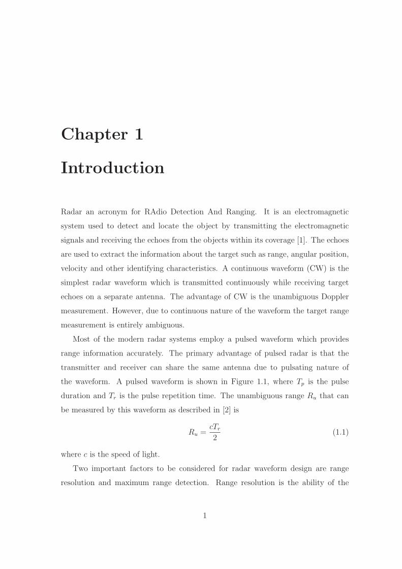
Most of the modern radar systems employ a pulsed waveform which provides

range information accurately. The primary advantage of pulsed radar is that the

transmitter and receiver can share the same antenna due to pulsating nature of

the waveform. A pulsed waveform is shown in Figure 1.1, where Tp is the pulse

duration and Tr is the pulse repetition time. The unambiguous range Ru that can

be measured by this waveform as described in [2] is

Ru =cTr

2(1.1)

where c is the speed of light.

Two important factors to be considered for radar waveform design are range

resolution and maximum range detection. Range resolution is the ability of the

1

Chapter 1 Introduction

Figure 1.1: Pulsed radar waveform

radar to separate closely spaced targets and it is related to the pulse width of the

waveform. The narrower the pulse width the better is the range resolution. But,

if the pulse width is decreased, the amount of energy in the pulse is decreased and

hence maximum range detection gets reduced. To overcome this problem pulse

compression techniques are used in the radar systems.

1.1 Pulse compression

The maximum detection range depends upon the strength of the received echo. To

get high strength reflected echo the transmitted pulse should have more energy for

long distance transmission since it gets attenuated during the course of transmission.

The energy content in the pulse is proportional to the duration as well as the peak

power of the pulse. The product of peak power and duration of the pulse gives an

estimate of the energy of the signal. A low peak power pulse with long duration

provides the same energy as achieved in case of high peak power and short duration

pulse. Shorter duration pulses achieve better range resolution. The range resolution

rres is expressed [2] as

rres =c

2B(1.2)

where B is the bandwidth of the pulse.

For unmodulated pulse the time duration is inversely proportional to the bandwidth.

If the bandwidth is high, then the duration of the pulse is short and hence this

offers a superior range resolution. Practically, the pulse duration cannot be reduced

indefinitely. According to Fourier theory a signal with bandwidth B cannot have

duration shorter than 1/B i.e. its time-bandwidth (TB) product cannot be less than

2


unity. A very short pulse requires high peak power to get adequate energy for large

distance transmission. However, to handle high peak power the radar equipment

become heavier, bigger and hence cost of this system increases. Therefore peak

power of the pulse is always limited by the transmitter. A pulse having low peak

power and longer duration is required at the transmitter for long range detection. At

the output of the receiver, the pulse should have short width and high peak power

to get better range resolution. Figure 1.2 illustrates two pulses having same energy

with different pulse width and peak power. To get the advantages of larger range

detection ability of long pulse and better range resolution ability of short pulse, pulse

compression [3] techniques are used in radar systems.

The range resolution depends on the bandwidth of a pulse but not necessarily on the

Figure 1.2: Transmitter and receiver ultimate signals

duration of the pulse [4]. Some modulation techniques such as frequency and phase

modulation are used to increase the bandwidth of a long duration pulse to get high

range resolution having limited peak power. In pulse compression technique a pulse

having long duration and low peak power is modulated either in frequency or phase

before transmission and the received signal is passed through a filter to accumulate

the energy in a short pulse. The pulse compression ratio (PCR) is defined as

PCR =width of the pulse before compression

width of the pulse after compression(1.3)

3


The block diagram of a pulse compression radar system is shown in Figure

1.3. The transmitted pulse is either frequency or phase modulated to increase the

bandwidth. Transreceiver (TR) is a switching unit helps to use the same antenna

as transmitter and receiver. The pulse compression filter is usually a matched filter

whose frequency response matches with the spectrum of the transmitted waveform.

The filter performs a correlation between the transmitted and the received pulses.

The received pulses with similar characteristics to the transmitted pulses are picked

up by the matched filter whereas other received signals are comparatively ignored

by the receiver.

Figure 1.3: Block diagram of a pulse compression radar system

1.2 Matched filter

In radar applications the reflected signal is used to determine the existence of the

target. The reflected signal is corrupted by additive white Gaussian noise (AWGN).

The probability of detection is related to signal-to-noise ratio (SNR) rather than

exact shape of the signal received. Hence it is required to maximize the SNR rather

4


than preserving the shape of the signal. A filter which maximizes the output SNR

is called matched filter [5]. A matched filter is a linear filter whose impulse response

is determined for a signal in such way that the output of the filter yields maximum

SNR when the signal along with AWGN is passed through the filter.

An input signal s(t) along with AWGN is given as input to the matched filter

as shown in Figure 1.4. Let N0/2 be the two sided power spectral density (PSD) of

AWGN. It is required to find out the impulse response h(t) or the frequency response

H(f) (Fourier transform of h(t)) that yields maximum SNR at a predetermined delay

t0. In other words, h(t) or H(f) is determined to maximize the output SNR which

is given by

Figure 1.4: Block diagram of matched filter

(

SP

NP

)

out

=|s0(t0)|2

n20(t)

(1.4)

where SP is the signal power, NP is the output noise power, s0(t0) is the value of

the output signal s0(t) at t = t0 and n20(t) is the mean square value of the noise.

If S(f) is the Fourier transform of s(t), then s0(t) is obtained as

s0(t) =

∫ ∞

−∞H(f)S(f)ej2πftdf (1.5)

The value of s0(t) at t = t0 is

s0(t0) =

∫ ∞

−∞H(f)S(f)ej2πft0df (1.6)

The mean square value n20(t) of the noise is evaluated as

n20(t) =

N0

2

∫ ∞

−∞|H(f)|2df (1.7)

5


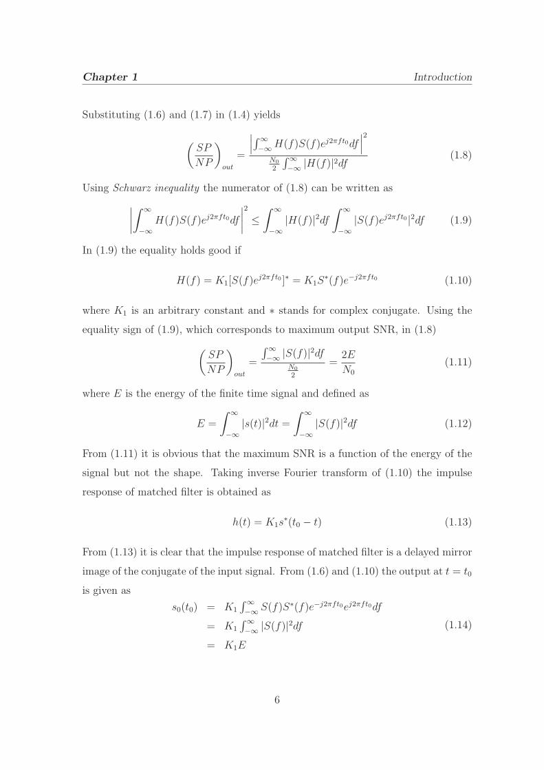
Substituting (1.6) and (1.7) in (1.4) yields

(

SP

NP

)

out

=

∣

∣

∣

∫∞−∞ H(f)S(f)ej2πft0df

∣

∣

∣

2

N0

2

∫∞−∞ |H(f)|2df (1.8)

Using Schwarz inequality the numerator of (1.8) can be written as

∣

∣

∣

∣

∫ ∞

−∞H(f)S(f)ej2πft0df

∣

∣

∣

∣

2

≤∫ ∞

−∞|H(f)|2df

∫ ∞

−∞|S(f)ej2πft0|2df (1.9)

In (1.9) the equality holds good if

H(f) = K1[S(f)ej2πft0 ]∗ = K1S∗(f)e−j2πft0 (1.10)

where K1 is an arbitrary constant and ∗ stands for complex conjugate. Using the

equality sign of (1.9), which corresponds to maximum output SNR, in (1.8)

(

SP

NP

)

out

=

∫∞−∞ |S(f)|2df

N0

2

=2E

N0

(1.11)

where E is the energy of the finite time signal and defined as

E =

∫ ∞

−∞|s(t)|2dt =

∫ ∞

−∞|S(f)|2df (1.12)

From (1.11) it is obvious that the maximum SNR is a function of the energy of the

signal but not the shape. Taking inverse Fourier transform of (1.10) the impulse

response of matched filter is obtained as

h(t) = K1s∗(t0 − t) (1.13)

From (1.13) it is clear that the impulse response of matched filter is a delayed mirror

image of the conjugate of the input signal. From (1.6) and (1.10) the output at t = t0

is given as

s0(t0) = K1

∫∞−∞ S(f)S∗(f)e−j2πft0ej2πft0df

= K1

∫∞−∞ |S(f)|2df

= K1E

(1.14)

6


Equation (1.14) states that regardless of the type of waveform, at the predefined

delay t = t0 the output is the energy of the waveform for K1 = 1. The output of the

matched filter is evaluated as

s0(t) = s(t) ⊗ h(t)

=∫∞−∞ s(τ)h(t − τ)dτ

=∫∞−∞ s(τ)K1s

∗(τ − t + t0)dτ

= K1=1,t0=0

∫∞−∞ s(τ)s∗(τ − t)dτ

(1.15)

where ⊗ denotes the linear convolution operation. The right hand side of (1.15) is

known as autocorrelation function (ACF) of the input signal s(t).

1.2.1 Matched filter for a narrow bandpass signal

Most of the radar signals are narrow bandpass signals. A narrowband signal s(t) [5]

can be represented as

s(t) =1

2u(t)ej2πf0t +

1

2u∗(t)e−j2πf0t (1.16)

where u(t) is the complex envelope of s(t) and f0 is the carrier frequency.

From (1.15) and (1.16)

s0(t) = K1

4

∫∞−∞[u(τ)ej2πf0τ + u∗(τ)e−j2πf0τ ]

{

u∗(τ − t + t0)e−j2πf0(τ−t+t0) + u(τ − t + t0)e

j2πf0(τ−t+t0)}

dτ(1.17)

Evaluating the products, (1.17) is represented as

s0(t) = K1

4ej2πf0(t−t0)

∫∞−∞ u(τ)u∗(τ − t + t0)dτ

+ K1

4e−j2πf0(t−t0)

∫∞−∞ u∗(τ)u(τ − t + t0)dτ

+ K1

4ej2πf0(t−t0)

∫∞−∞ u∗(τ)u∗(τ − t + t0)e

−j4πf0τdτ

+ K1

4e−j2πf0(t−t0)

∫∞−∞ u(τ)u(τ − t + t0)e

j4πf0τdτ

(1.18)

In (1.18) the second and fourth terms of right hand side are the complex conjugate

of first and third terms respectively. So it can be written as

s0(t) = K1

2Re{

ej2πf0(t−t0)∫∞−∞ u(τ)u∗(τ − t + t0)dτ

}

+ K1

2Re{

ej2πf0(t−t0)∫∞−∞ u∗(τ)u∗(τ − t + t0)e

−j4πf0τdτ} (1.19)

7


The second term on the right hand side of (1.19) is the Fourier transform of

u∗(τ)u∗(τ − t+ t0) evaluated at f = 2f0, which is at much higher frequency than the

spectrum of the complex envelope u(t). So neglecting the second term the expression

in (1.19) becomes

s0(t) = K1

2Re{

ej2πf0(t−t0)∫∞−∞ u(τ)u∗(τ − t + t0)dτ

}

= Re{[

K1

2e−j2πf0t0

∫∞−∞ u(τ)u∗(τ − t + t0)dτ

]

ej2πf0t} (1.20)

The expression inside the square bracket of (1.20) is defined as new complex envelope

u0(t) which is expressed as

u0(t) = K2

∫ ∞

−∞u(τ)u∗(τ − t + t0)dτ (1.21)

where K2 = K1

2e−j2πf0t0 .

The output of the matched filter is

s0(t) = Re{

u0(t)ej2πf0t

}

(1.22)

From (1.21) and (1.22) it is observed that the matched filter output of narrow

bandpass signal has a complex envelope u0(t) which is obtained by passing the

complex envelope u(t) through its own matched filter.

1.2.2 Matched filter response to Doppler shifted signal

Most of the targets in the environment are non stationary. So the frequency of

the reflected signal from a target experiences Doppler shift. The Doppler shifted

complex envelope is represented as

uD(t) = u(t)ej2πfdt (1.23)

where fd is the Doppler shift.

Substituting uD(t) for first u(t) in (1.21) and choosing t0 = 0 and K2 = 1

u0(t, fd) =

∫ ∞

−∞u(τ)ej2πfdτu∗(τ − t)dτ (1.24)

8


Reversing the operations of τ and t a modified expression obtained as

χ(τ, fd) =

∫ ∞

−∞u(t)u∗(t − τ)ej2πfdtdt (1.25)

Equation (1.25) is one of the versions of the ambiguity function (AF). The AF

describes the output of the matched filter if the input signal is delayed by τ and

Doppler shifted by fd relative to the values for which the matched filter is designed.

The AF was introduced by Woodward [6] which is an important tool for radar

signal analysis. But the AF expressions given in [2,4–6] differ in the sign of τ and fd.

τ gives the information whether the target is farther from or nearer to the reference

and fd gives the information whether the target is moving towards or moving away

from the radar. A standard form of AF which is used in most of the radar systems

is

|χ(τ, fd)| =

∣

∣

∣

∣

∫ ∞

−∞u(t)u∗(t + τ)ej2πfdtdt

∣

∣

∣

∣

(1.26)

where a positive τ corresponds to the target being farther from the radar and a

positive fd corresponds to the target moving towards the radar.

1.2.3 Properties of ambiguity function

Some of the important properties of AF [5] are explained below where energy of u(t)

normalized to unity .

1. It has maximum value at origin (0,0) i.e.

|χ(τ, fd)| ≤ |χ(0, 0)| = 1 (1.27)

2. The total volume under AF is unity and independent of signal waveform.

∫ ∞

−∞

∫ ∞

−∞|χ(τ, fd)|2 dτdfd = 1 (1.28)

3. AF is symmetrical with respect to origin

|χ(τ, fd)| = |χ(−τ,−fd)| (1.29)

9


4. If a complex envelope u(t) has AF |χ(τ, fd)| then addition of linear frequency

modulation, which is equivalent to a quadratic phase modulation, makes the

AF as

u(t)ejπkt2 ⇔ |χ(τ, fd − kτ)| (1.30)

1.2.4 Cuts through ambiguity function

1. Cuts along the delay axis

The cut along the delay axis is obtained by setting fd = 0 in (1.26) i.e.

|χ(τ, 0)| =

∣

∣

∣

∣

∫ ∞

−∞u(t)u∗(t + τ)dt

∣

∣

∣

∣

= |R(τ)| (1.31)

where R(τ) is the autocorrelation function of u(t).

2. Cuts along the Doppler axis

Setting τ = 0 in (1.26) yields

|χ(0, fd)| =

∣

∣

∣

∣

∫ ∞

−∞|u(t)|2ej2πfdtdt

∣

∣

∣

∣

(1.32)

Equation (1.32) states that the cut along the Doppler axis yields the Fourier

transform of the magnitude of the square of the complex envelope u(t).

1.3 Radar signals

In radar system a particular waveform is first determined for a given application and

it is used to design the optimum detection system. The waveform should provide

least amount of uncertainty or ambiguity when the reflected signal is used to extract

the information about the range, the velocity and the number of true targets present

in the environment. The different types of signals those are mostly used in radar

systems are discussed in sequel.

10


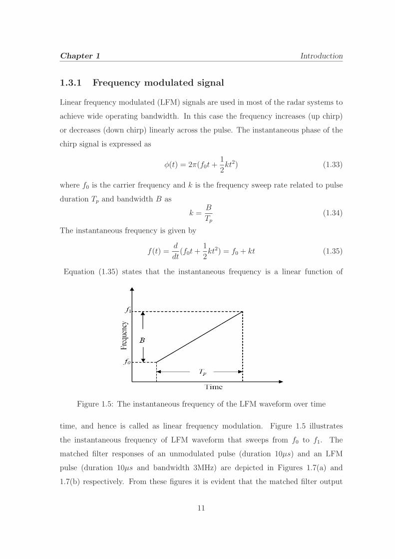
1.3.1 Frequency modulated signal

Linear frequency modulated (LFM) signals are used in most of the radar systems to

achieve wide operating bandwidth. In this case the frequency increases (up chirp)

or decreases (down chirp) linearly across the pulse. The instantaneous phase of the

chirp signal is expressed as

φ(t) = 2π(f0t +1

2kt2) (1.33)

where f0 is the carrier frequency and k is the frequency sweep rate related to pulse

duration Tp and bandwidth B as

k =B

Tp

(1.34)

The instantaneous frequency is given by

f(t) =d

dt(f0t +

1

2kt2) = f0 + kt (1.35)

Equation (1.35) states that the instantaneous frequency is a linear function of

Figure 1.5: The instantaneous frequency of the LFM waveform over time

time, and hence is called as linear frequency modulation. Figure 1.5 illustrates

the instantaneous frequency of LFM waveform that sweeps from f0 to f1. The

matched filter responses of an unmodulated pulse (duration 10µs) and an LFM

pulse (duration 10µs and bandwidth 3MHz) are depicted in Figures 1.7(a) and

1.7(b) respectively. From these figures it is evident that the matched filter output

11


of LFM signal has narrow mainlobe width and hence has better range resolution

capability. However it is associated with sidelobes which are unwanted in output

from the filter. The compressed pulse width of LFM signal is 1/B and the PCR is

obtained as

PCR = BTp (1.36)

1.3.2 Phase coded signal

The increase in bandwidth can also be achieved by phase modulation. In this case a

long pulse width Tp is divided into a number of sub pulses each of width tb as shown

in Figure 1.6. Each sub pulse is assigned with a phase value φi, where i = 1, 2, ...N .

The received echo is passed through a filter to get a single output peak. The most

popular phase coding is biphase or binary coding. A biphase code consists of a

sequence of +1 and -1. The phases of the transmitted waveform is 00 for +1 and

1800 for -1. The coded signal is discontinuous at the point of phase reversal. The

matched filter response of a randomly assigned 10-bit biphase code ([1 -1 1 -1 1 -1

-1 1 1 -1]) is shown in Figure 1.7(c). It is evident from the figure that phase coded

signals are also associated with the sidelobes. The PCR of phase coded pulse is

obtained as

Figure 1.6: Phase modulated waveform

PCR =Tp

tb(1.37)

Figure 1.7 shows that the modulated signals provide better range resolution as

compared to unmodulated signals but the matched filter output of the modulated

signals suffer from the sidelobes. These sidelobes may hide the small targets or may

cause false target detection. The sidelobe having largest amplitude is called peak

12


−1 −0.8 −0.6 −0.4 −0.2 0 0.2 0.4 0.6 0.8 1

x 10−5

0

0.2

0.4

0.6

0.8

1

Delay time

|AC

F|

(a) Matched filter response for unmodulated pulse

−1 −0.8 −0.6 −0.4 −0.2 0 0.2 0.4 0.6 0.8 1

x 10−5

0

0.2

0.4

0.6

0.8

1

Delay time

|AC

F|

Sidelobes

Mainlobe

(b) Matched filter response for frequency modulated pulse (TB = 30)

0 2 4 6 8 10 12 14 16 18 200

0.2

0.4

0.6

0.8

1

Delay time

|AC

F|

Sidelobes

Mainlobe

(c) Matched filter response for phase modulated pulse

Figure 1.7: Matched filter output of different signals

13


Table 1.1: Barker codes

Code length Coded signal PSR in dB2 1-1,-11 -63 11-1 -9.54 11-11,111-1 -125 111-11 -147 111-1-11-1 -16.911 111-1-1-11-1-11-1 -20.813 11111-1-111-11-11 -22.3

sidelobe. The lower the peak sidelobe level (PSL) the better is the code. To quantify

the the waveform characteristics peak to sidelobe ratio (PSR) and integrated sidelobe

ratio (ISR) are used as measures of performance in radar systems. These are defined

as

PSR = 10 log10peak sidelobe power

mainlobe power(1.38)

ISR = 10 log10total power in sidelobes

mainlobe power(1.39)

In biphase codes the selection of random phase 0 or π is a difficult task. The phases

are selected so that the matched filter output of the code has lower sidelobes. Barker

codes are the special type of binary codes having sidelobes of unity magnitude.

Exhaustive computer based search reveals that the Barker codes are available for

the length of 2, 3, 4, 5, 7, 11 and 13 only. The Barker codes along with their PSR

values are listed in Table 1.1. The Barker code have maximum compression ratio is

13 and highest PSR magnitude is 22.3 dB.

A longer code is required for many radar application to achieve high pulse

compression ratio. One way to obtain a longer code having lower sidelobe level

is by nesting two Barker codes using Kronecker product. This type of code is called

compound Barker code. If one Barker code has length l1 and that of other is l2,

then the compound Barker code is of length l1l2 and the compression ratio is l1l2.

For example a 35-bit compound Barker code is generated by taking the Kronecker

tensor product of 5-bit and 7-bit Barker codes and the resultant code is [1 1 1 -1 -1

14


1 -1 1 1 1 -1 -1 1 -1 1 1 1 -1 -1 1 -1 -1 -1 -1 1 1 -1 1 1 1 1 -1 -1 1 -1]. Although a larger

compression ratio is achieved by compound Barker code, the peak sidelobes are not

proportionally decreased. The codes those yield minimum peak sidelobe level but

do not meet the Barker condition (i.e. maximum PSL is unity) are called minimum

peak sidelobe (MPS) level codes.

If the pulse is allowed to take more than two values, it is known as a polyphase

code. The phases of the polyphase code are chosen in such way that its ACF should

have lower sidelobes. However the polyphase codes are sensitive to Doppler shift.

To overcome this problem the polyphase codes are derived from the phase history

of the frequency modulated pulses. The details of polyphase codes and their pulse

compression methods are discussed in Chapter 4.

1.4 Background and scope of the thesis

A lot of research work has been carried out over past few decades to achieve low

sidelobes and high range resolution in the radar pulse detection system [5]. Biphase

coding techniques are preferred in pulse compression techniques owing to their easy

implementation. The phases of biphase codes are assigned randomly to different

bits of a certain length of code according to different measure of performance. So

efficient techniques are required to assign the phases of biphase codes such that it

would provide better performance indices.

Practically the mismatch filters are used to provide better PSR, with some SNR

loss, than matched filter. Various mismatch filters such as adaptive linear combiner

(ALC) and neural networks are used to suppress the sidelobes [38,39,41]. However,

the convergence of the neural network is slow during the training period. Hence

new efficient structures and the corresponding learning algorithms having faster

convergence are required for pulse compression.

Apart from biphase codes, polyphase codes [80, 81] and frequency modulated

codes are also used in radar systems. In the literature different type of windows

are used as weighing function to suppress the sidelobes [89, 90] of polyphase codes

15


and LFM waveforms [71]. Under the Doppler shift conditions the PSR magnitude

provided by the windows are low. Hence efficient amplitude weighing techniques are

needed to achieve lower sidelobes in Doppler shift conditions.

In phased array radar, wide bandwidth waveforms are used to acquire high

range resolution. Generation of such types of waveforms increases the overall cost

and complexity of the system. The conventional hardware designed for narrowband

signals in radar systems may not sustain instantaneous wide bandwidth. To

overcome such limitation the wide bandwidth signal is split into a set of narrowband

signals which are transmitted and received separately. The effect of wideband

signal is obtained by coherently combining the narrowband signals. Such type

of narrowband signals taken together is called ‘synthetic wideband waveform’ or

‘stepped frequency waveform’ or ‘frequency jumped train’. However, the matched

filter output i.e. ACF of such signals suffers from grating lobes due to constant

frequency step. Therefore there is a need to design a signal having wide bandwidth

but can be processed by the hardware for narrow band signals and its ACF has

suppressed grating lobe, low peak sidelobes and narrow mainlobe width.

1.5 Motivation

Substantial effort has been made to suppress the sidelobes of the different waveforms

using computational intelligence (CI) tools such as evolutionary computing

techniques and neural networks.

• Several existing evolutionary computing techniques have been employed to

assign the phase to different bits of biphase codes using weighted sum of PSL

and merit factor (MF) as cost function [14, 15]. The problem associated with

these methods is to choose the appropriate values of the weights.

• The matched filter does not provide adequate PSR for many radar applications.

Hence to obtain improved PSR, the mismatch filters have been introduced

whose weights are adapted using known input output data. Various mismatch

16


filters using multilayer perceptron (MLP) and radial basis function (RBF)

networks have been reported in the literature. However these filters provide

poor convergence performance and hence the magnitude of PSR is less during

detection. Thus there is need to design improved mismatch filters.

• For polyphase and LFM waveforms the amplitude weighing techniques are

used at the receiver to suppress sidelobes. The targets in the environment

are not always stationary. If the target is in motion, the reflected waveform

is Doppler shifted version of the transmitted waveform. When this Doppler

shifted waveforms are passed through the weighted receiver matched filter the

PSR degrades. Under such situations it is required to improve the PSR.

• The matched filter output i.e. ACF of wide bandwidth stepped frequency LFM

pulse train suffers from grating lobes due to constant frequency step. Several

methods have been implemented to suppress the grating lobes in [113, 114].

These methods generally ignore the PSL and mainlobe width which are

also important measures of the performance for target detection. Therefore,

algorithms need to be developed to choose the parameters of stepped frequency

waveform such that the output of the matched filter provides high range

resolution, lower grating lobes and reduced sidelobes.

Based on the aforementioned motivations, the objectives of the research work of

this thesis is developed. The thesis employs evolutionary, soft computing and signal

processing techniques to solve these problems of pulse compression.

1.6 Objective of the thesis

The main objective of present research work is to propose efficient pulse compression

techniques for different radar signals. The various objectives may be listed as:

• To generate pulse compression biphase codes having lower peak sidelobes and

better MF using multiobjective algorithm.

17


• To develop efficient sidelobe reduction structures using neural networks which

converge faster during the training time as well as provide higher magnitude

of PSR.

• To introduce and assess amplitude weighing technique for LFM waveform and

polyphase codes which is expected to provide better PSR at higher Doppler

shifts.

• To select appropriate parameters of LFM pulse train to achieve reduced grating

lobes, low peak sidelobe level and narrow mainlobe width.

1.6.1 Structure and chapter wise contribution of the thesis

Chapter-1

The concept of pulse compression, matched filter, ambiguity function and

different radar signals are introduced in this chapter. The motivation behind the

application of evolutionary, neural network and signal processing techniques for

pulse compression is outlined. The summary of framework of the research and

contributions are also included.

Chapter-2

In this chapter the biphase codes having lower PSL and better MF in their ACFs

are generated. Genetic algorithm (GA) is used to optimize a cost function consisting

of weighted combination of PSL and MF. However there is difficulty in selection of

proper weight value to optimize the combination. In order to overcome this difficulty

a multiobjective algorithm (based on nondominated sorting genetic algorithm-II

(NSGA-II) ) is proposed which simultaneously optimize the PSL and MF. The

proposed algorithm provides a set of nondominated solutions. Simulations have

been carried out using proposed algorithm to generate pulse compression biphase

codes for length 49 to 59. NSGA-II provides more than one nondominated codes

for each length. A particular code of specified length is chosen in accordance to

the requirement of the environmental condition. If the environmental condition is

18


dominated by distributed clutter then the code having high MF is preferred. On

the other hand if the application requires the detection of target in presence of large

discrete clutter the code having low PSL is chosen.

Chapter-3

Several mismatch filters are investigated in this chapter which provide better PSR

values as compared to the matched filter. The best binary codes available in

the literature are known as Barker codes having maximum sidelobe level of unity

amplitude. The largest Barker code available is of length 13 having a PSR of

magnitude 22.3 dB which is not adequate for many radar applications. The Barker

codes of larger length are generated by taking Kronecker product of existing Barker

codes. To obtain higher PSR value the mismatch filters such as adaptive linear

combiner, multilayer perceptron (MLP) and radial basis function (RBF) along

with their learning algorithms are investigated. The convergence performance of

MLP and RBF structures is very slow. Therefore recurrent neural network (RNN)

and recurrent RBF (RRBF) structures capable of yielding faster convergence are

proposed for the pulse compression filter. The shifted version of 13-bit and 35-bit

Barker codes are used as input to the different networks. The desired output of

the network is always zero except at one point corresponding to the presence of

target. The convergence rate during training for RNN and RRBF are compared to

that of MLP and RBF networks. After the training is complete the networks are

used for pulse radar detection. The PSR values of RRN and RRBF for different

noise conditions, presence of multiple target and under Doppler shift condition are

evaluated and compared with those of MLP and RBF.

Chapter-4

This chapter presents pulse compression for LFM waveforms and polyphase codes.

The LFM and polyphase codes have lower sidelobes compared to the biphase codes.

LFM waveforms are more Doppler tolerant than phase coded waveforms. Polyphase

codes are derived from the LFM waveform to get the advantage of the Doppler

tolerant property of the LFM waveform. The matched filter output of the LFM

19


waveform yields PSR of -13.2 dB. Different weighing functions are used in the

receiver to achieve high PSR magnitude and the LFM waveform is amplitude tapered

or phase distorted before transmission to get even higher PSR magnitude. The

weighing functions are also used for sidelobe suppression of polyphase codes. If

the target is in motion then the reflected signal is Doppler shifted version of the

transmitted signal. In this chapter convolutional windows are proposed to use as

weighing function for LFM and polyphase codes to achieve better PSR values in

Doppler shift conditions. Simulation study is carried out to assess the performance

of the convolutional windows and is compared to those of conventional windows.

Chapter-5

In this chapter evolutionary computing techniques are proposed to determine

the parameters of stepped frequency LFM pulse train. In case of high range

resolution radar the required bandwidth is very high. The conventional narrowband

hardware may not support the instantaneous wide bandwidth. Therefore, the

wide bandwidth signal is split into narrowband signals which are transmitted and

combined coherently at receiver to get the effect of the wideband signal. But the

ACF of such narrow band pulse train suffers from grating lobes and hence destroys

the range resolution capability of the pulse train. In the proposed work the particle

swarm optimization (PSO) technique is used to determine the parameters of the LFM

pulse train such that all the grating lobes are cancelled. Apart from cancellation

or suppression of grating lobe, minimization of mainlobe width and peak sidelobe

level of ACF are also important for the radar systems. In this chapter NSGA-II

algorithm is proposed to choose the parameters of stepped frequency LFM pulse

train to accomplish reduced grating lobes, low peak sidelobe and narrow mainlobe

width.

Chapter-6

In this chapter the overall contributions of the thesis are reported. This chapter also

contains the details of further research work which can be attempted subsequently.

20


1.7 Conclusion

This chapter provides a brief introduction to radar, pulse compression technique and

different signals used in radar. The merits and demerits of the pulse compression

technique are studied. It also systematically outlines the scope, the motivation

behind this work and the objectives of the thesis. In essence, this chapter provides

an overview of the thesis in a comprehensive manner.

21

Chapter 2

Generation of Pulse CompressionCodes Using MultiobjectiveGenetic Algorithm

2.1 Introduction

In a pulse radar system the transmitted pulse width should be as long as possible to

increase the sensitivity of the system and as small as possible at the receiver for better

range resolution. Range resolution is the ability of the radar receiver to discriminate

nearby targets. The performance of range resolution radar would be optimal, if the

coded waveform has impulsive ACF. Biphase coded waveforms support better range

resolution compared to LFM pulses because the windowing functions used with LFM

pulses to lower time sidelobes cause a broadening in the mainlobe. But the ACF

of biphase coded waveforms contain higher range sidelobes, which have a negative

influence on the detection performance of radar systems. A desirable property of

the compressed pulse is that it should have low sidelobes in order to prevent a

weaker target from being masked in the sidelobes of a nearby stronger target. The

lower the sidelobes relative to the mainlobe peak, the better the main peak can be

distinguished and hence the better is the corresponding code. The selection of a pulse

compression code depends on the application and the environmental conditions. If

the application is radar designed for a scenario dominated by distributed clutter,

then integrated sidelobe level (ISL) is very important. On the other hand if the

22

Chapter 2

Generation of Pulse Compression

Codes Using Multiobjective Genetic Algorithm

application requires detection of targets in the presence of large discrete clutter, then

the PSL is more important. If the desired ISL or PSL performance is not achieved

with a matched filter, a mismatch filter is used to achieve the desired sidelobe level

with some SNR loss.

Binary pulse compression codes [7] such as the Barker codes [8] or maximal-length

sequences [9] are extensively used in radar systems. The Barker codes which are

known as the best ideal waveform can provide a maximum PCR of 13. Many

practical applications require longer codes to achieve higher PCRs much greater

than 13. Therefore sequences with the lowest possible sidelobes at the longer length

are needed. There is no analytical technique available to construct a sequence for

a given PSL. Time consuming and money consuming exhaustive computer search

program are generally used to generate best possible sequences. By exhaustive

computer search program, Lindner [10] found all binary sequences up to length 40

with minimum PSL. With an improved algorithm Cohen et al. [11] further extended

those results to sequence length 48. For larger sequences some heuristic methods,

such as neural network (NN) and evolutionary algorithms (EAs) are proposed to

search the binary sequences with good aperiodic autocorrelation [12–15]. Using an

NN approach, Hu et al. [12] obtained useful binary sequences for lengths 49 up to 100.

An objective function which consists of weighted sum of PSL and merit factor (MF)

is optimized using genetic algorithm (GA) to generate codes from 49 to 100 [15]. The

demerit of this type of objective function is to choose the accurate weight values. It

is also required to run the program repeatedly for different combinations of weight

values. To overcome this problem, in the proposed work a multiobjective algorithm

is introduced in which PSL and MF are used as two different objective functions to

generate the biphase codes.

23

Chapter 2



2.2 Merit measures and problem formulation

Let an L length binary sequence is given by

S = {s1, s2, s3, · · · , sL} (2.1)

where each element of S has a value either +1 or -1.

The ACF of S for positive delays is given as

Ck(S) =L−k∑

i=1

sisi+k (2.2)

where k = 0, 1, 2, · · · , L − 1.

Ideally, the range resolution radar signal should have high ACF value for zero shift

and zero value for nonzero shift. A significant problem inherent in biphase pulse

compression is that the ACF does not yield a perfect impulse, that means it does

not produce Ck(S) = 0 for k 6= 0. Any non zero value of Ck(S) for k 6= 0 is referred

to as sidelobe where as the zero-offset correlation value C0(S) is called the mainlobe.

The difference between a pulse compression waveform and a simple pulse waveform

lies in the existence and magnitude of these sidelobes. These sidelobes limit the

usefulness of a code regardless of the strength of the mainlobe. Codes are chosen for

a given application based on their length and sidelobe levels.

There are two main criteria [16, 17] used to decide the goodness of a pulse

compression code. The first one is the PSL which is the largest sidelobe in the

ACF of the code and defined as

PSL = Max |(Ck(S))| , k 6= 0 (2.3)

The second one is the merit factor MF which is defined as the ratio of energy in

the main peak of the ACF to the total energy in the sidelobes. As the signal is real

valued the ACF is real and symmetric about the zero delay. The MF is represented

as

MF =C2

0(S)

2∑L−1

k=1 C2k(S)

(2.4)

24

Chapter 2



The denominator of (2.4) is known as ISL. For a good sequence or code the PSL

should be low and MF should be high. To optimize simultaneously PSL and MF

using GA, the fitness function is defined as

f =α

PSL+ βMF (2.5)

The fitness function f is maximized using suitable values of α and β such that

α + β = 1. However it is a difficult task to choose a proper combination of α and β

to get a optimized code. Hence in the proposed work nondominated sorting genetic

algorithm -II (NSGA-II) is used to optimize multiple objective functions PSL and

MF simultaneously to generate biphase pulse compression codes.

2.3 Techniques used

The techniques which are used to generate pulse compression codes are described in

this section.

2.3.1 Genetic algorithm

The GA is a programming technique that mimics biological evolution process and

uses the genetic operators such as selection, crossover and mutation for problem

solving strategy. GAs are based on Darwin’s theory of evolution i.e. the strong

survivors have better opportunity to transfer their genes to future generations

through reproduction. Species those carry correct combination in their genes are

dominant in the population. Sometimes during the process of evolution, random

changes may occur in genes. If these changes render advantages for the survival,

new species evolve from the old ones. In other words unsuccessful changes are

eliminated by the natural selection.

The GA was originally proposed by J. Holland [18] in 1975 which imitates

nature’s robust way of evolving successful organisms. Afterwards it became popular

due to the publication of D. Goldberg’s book in 1989 [19]. Since then the GAs have

been used in a wide range of applications where optimization is needed. In the GA,

25

Chapter 2



a solution is called as an individual or chromosome and each element of chromosome

called as genes. The GA works on a set of chromosomes called as a population. As

the search evolves, the population have fitter and fitter solutions. The various steps

involved in the GA are follows

1. Population initialization

Population size is the number of chromosomes required in one generation. If there

are too few chromosomes, GA have a few possibilities to perform crossover and only

a small part of the search space is explored. On the other hand, if there are too many

chromosomes, GA process will slow down. A chromosome is represented in such a

way that it should contain information about the solution. The chromosomes are

presented in real numbers such as 0.5, -0.3, 1.5 etc or encoded to binary form, using

an encoding process, such as ‘1001010101’, ‘1001001010’ etc. This chapter is dealt

with only binary representation of the chromosomes. M number of chromosomes

are randomly initialized with binary forms.

2. Fitness function evaluation

The initialized population is used to evaluate the objective function which is to be

optimized. This is known as fitness function evaluation since the objective function

value corresponds to the fitness of that chromosome.

3. Selection

Chromosomes from the population are selected by using a mechanism to enter into

a mating pool. Chromosomes from the mating pool are used to produce offspring

which form the basis for the next generation. As the genes of the chromosome

are to be inherited to the next generation, it is desirable the mating pool should

contains good chromosomes. So a selection procedure in GA is used to select

better individuals in the population for the mating pool. The selection pressure

is the degree to which the better chromosomes are favored. The higher the selection

26

Chapter 2



pressure, the more the better individuals are favored. Selection pressure helps GA

to improve the population fitness over succeeding generations.

There are many selection methods available in the literature such as roulette

wheel, tournament, rank and steady state selection [20] etc. In this thesis a binary

tournament selection is used to choose a chromosome from the population. In this

selection a tournament size consisting of two chromosomes are randomly chosen

and the winner of the two is the chromosome with the highest fitness value. The

winner is entered into the mating pool. As the mating pool comprised of tournament

winners, it has a higher average fitness than average population fitness. This fitness

difference provides the selection pressure, which helps GA to improve the fitness of

each succeeding generation.

4. Genetic operators

Genetic operators such as crossover and mutation are used to explore and exploit new

and better solutions from the existing solutions in the search space. The operators

are explained below.

a. Crossover

In this operation two chromosomes, called parents, are selected using binary

tournament selection from the existing population and combined together to form

new chromosomes. These newly formed chromosomes are called offspring. It is

always expected that offspring inherits good genes from the parent. A single point

crossover and a two point crossover are shown in Figure 2.1. In case of single point

crossover a point is randomly selected and all the genes after this point are swapped

between the two parent chromosomes to form two offspring. Similarly, in case of two

point crossover two points are randomly selected and the genes in between the two

points are swapped between the two parents to form two offspring. This operation

is carried out with certain probability called as crossover probability which indicates

how often crossover will be performed. If there is a crossover, offspring is made from

parts of parents chromosome. If crossover probability is 100%, then all offspring is

27

Chapter 2



(a) Single Point Crossover

(b) Two Point Crossover

Figure 2.1: Crossover

made by crossover. If it is 0%, whole new generation is made from exact copies of

chromosomes from old population. Crossover is made in hope that new chromosomes

will contain good parts of the old chromosomes and therefore the new chromosomes

are better. However it is good to leave some part of the old population survive to

next generation.

b. Mutation

It takes place at the gene level. It introduces random changes into the features of

chromosomes. In GA the probability of mutation is smaller in comparison to the

probability of crossover. If there is no mutation, offspring is taken after crossover

(or copy) without any change. If mutation is performed, part of chromosome is

changed. If mutation probability is 100%, whole chromosome is changed and if

it is 0%, nothing is changed. Mutation reintroduces the genetic diversity back

28

Chapter 2



into the population and helps to escape from the local minima. In case of binary

representation of codes a randomly chosen bit is switched from 1 to 0 or 0 to 1 as

shown in Figure 2.2.

Figure 2.2: Mutation

5. Recombination and selection

This process is used to weed out the weaker chromosomes from the population so

that the more productive chromosomes will be used in the next generation. In most

of the cases the fitness function value of a chromosome decides its survival for the

next generation. The current generation population is combined with the offspring

population and the fitness values of each chromosome of the combined population

is evaluated. The best M chromosomes are selected according to the fitness value

to carryout the next generation.

A flow chart for GA operation is depicted in Figure 2.3.

2.3.2 Multi objective GA

In single objective problems one has to find out the best solution which is usually the

global maximum or minimum relying on the problem. In practice, the optimization

problem is associated with multiple, possibly conflicting, objectives and this type

of problem may not have one best solution with respect to all the objectives. A

set of solutions exists in the search space which are superior to rest of the solutions

with respect to all the objectives but are inferior among themselves with respect

to one or more objectives. These solutions are called as nondominated solutions or

Pareto optimal solutions. None of the nondominated solutions is better than the

29

Chapter 2



Figure 2.3: Flow chart for GA

30

Chapter 2



other or in other words every solution is an acceptable solution. The superiority

of one solution over the other depends upon the knowledge of the problem and its

application. Thus, a solution chosen by a designer may not be accepted by another.

A multiple objectives problem can be solved as a single objective problem by

assigning a weight wi to each objective as follows: minimize

z = w1z1(x) + w2z2(x) + ..... + wkzk(x) (2.6)

where z1(x), z2(x), ....zk(x) are the objective functions and∑k

i=1 wi = 1.

In this approach a single set of weight vector produces a single solution. If

multiple solutions are required the problem has to run repeatedly for different

set of weights. The drawback of this type of approach is judicious selection of a

weight vector for each solution, which is a difficult task. To overcome this difficulty

many multiobjective evolutionary algorithms are found in literature to get a set of

nondominated solution in a single run. In [21–26], the evolutionary algorithms are

amply demonstrated and it is found that these are efficient to find multiple and

diversified nondominated solutions. The difference between single objective GA and

multiobjective GA (MOGA) is the concept of dominance used directly or indirectly

in the selection phase of MOGA. The effective MOGA approximates the true Pareto

front and maintains diversity in the population [21]. Schaffer [22] has proposed the

first practical multiobjective algorithm, called as vector evaluated GA (VEGA). This

algorithm solves each objective separately and then combines sub solution of each

objective. One of the demerits of this algorithm is that it is biased towards some

of the Pareto optimal solutions. In [23], an MOGA is proposed which explores the

solution in all possible directions in the search space. Subsequently many GAs have

been proposed by many researchers to find out improved nondominated solutions in

the objective space. These algorithms are efficient in terms of complexity, rate of

convergence, diversity among the nondominated solution and the interval distance

from the Pareto optimal front. Deb and Srinivas [25] have proposed a robust

popular nondominated sorting genetic algorithm (NSGA) to solve multiobjective

optimization problems. But this algorithm involves high computational complexity,

31

Chapter 2



lacks elitism and difficulty in choosing the optimal value of sharing parameter. An

improved version of NSGA, called NSGA-II, is dealt in [26] which uses the concept

of elitism and does not use the sharing parameter. The various steps of NSGA-II

algorithm are given below.

1. Population initialization:

The population contains a set of M chromosomes. Each chromosome is initialized

randomly with binary bits.

2. Fitness function evaluation:

The fitness functions which are to be optimized are evaluated for each chromosome.

3. Nondominated sort:

The initialized population is sorted according to nondomination. The sorting

algorithm [26] is given below.

• for each solution x in the main population X do the following

– the domination counter nx, the number of solution that dominate the

solution x, is initialized as zero i.e nx = 0.

– Sx, a set which contains all the solutions to those the solution x dominates,

is initialized as an empty set φ i.e. Sx = φ

– for each solution y in X

∗ if x dominates y

· y is added to the set Sx i.e Sx = Sx ∪ {y}.

∗ else if y dominates x then

· the domination counter of x is incremented i.e. nx = nx + 1.

– if nx = 0 i.e. no solution dominates x then it belongs to the first front.

Assign rank one to the solution i.e. xrank = 1. The first front is updated

by adding x to it i.e. F1 = F1 ∪ {x}.

32

Chapter 2



• This process is executed for all solutions in X.

• The front counter i is initialized to one i.e. i = 1.

• The following steps will be executed until ith front is non empty i.e.Fi 6= φ.

– A set Y = φ is defined to store the solutions for next front.

– for each solution x in front Fi

∗ for each solution y in Sx

· ny = ny − 1, the domination count for solution y is decreased.

· if ny = 0, then y belongs to the next front. Hence yrank = i + 1.

The set Y is updated as Y = Y ∪ {y}.

– The front counter incremented by one i.e. i = i + 1.

– Y is set as next front i.e. Fi = Y .

4. Crowding distance:

An efficient multiobjective algorithm not only converges to the true Pareto optimal

set but also requires good spread or diversity among the obtained solutions. The

original NSGA [25] uses a sharing parameter to achieve the diversity among the

solutions. The difficulties of this algorithm are choosing the sharing parameter value

and associated heavy computational complexity. These difficulties are overcome in

NSGA-II by providing better diversity among the solutions using the concept of

crowding distance. It does not require any user defined parameter to maintain the

diversity among the solutions. The crowding distance is calculated front wise as

follows.

• For any front Fi, l is the number of solutions i.e. |Fi| = l.

– The distance of all the solutions are initialized to zero i.e. Fi(Dj) = 0,

where the index j corresponds to jth solution in front Fi.

– for each objective function m

33

Chapter 2



∗ The solutions in front Fi are sorted in ascending order according to

the objective function value i.e. I = sort(Fi,m)

∗ Infinite distance value is assigned to the boundary solutions of front

Fi i.e. Fi(D1) = Fi(Dl) = ∞

∗ for j = 2 to l − 1

Fi(Dj) = Fi(Dj) + I(j+1)·m−I(j−1)·mfmax

m −fminm

where I(j) · m is the mth objective function value of jth solution in

I. fminm and fmax

m are minimum and maximum value of mth objective

function.

• The above procedure is carried out for all the fronts.

The solution that has large crowding distance value means it is far away from others,

hence it is selected first.

5. Selection:

a. Based on nondomination rank: A solution is selected if its nondomination rank

is lower than other.

b. Based on crowding distance: If two solutions belong to the same front, the solution

having higher crowding distance is selected.

The selection procedure is used during binary tournament selection and population

reduction phase.

6. Genetic operators:

These operators are used to produce offspring from the parent. The process of

crossover and mutation are carried out as explained in Section 2.3.1

7. Recombination and selection:

The current generation population is combined with the offspring population and

selection is carried out to choose the best M solutions for next generation. In this

34

Chapter 2



algorithm elitism is ensured as all the previous population is added with the current

population for selection process. The algorithm for selection process is given below.

• Let Ag and Bg are current and offspring population respectively of gth

generation. The combined population Cg = Ag + Bg.

• Sort the population Cg according to nondominated sort and determine all the

fronts (F1, F2, ....).

• Initialize i = 1

• The following is carried out until (|Cg+1| + |Fi|) ≤ M

– Assign the crowding distance to the solutions of the front Fi.

– Update Cg+1 by adding all solutions of Fi to it i.e. Cg+1 = Cg+1 ∪ Fi.

– i = i + 1.

• Sort the solutions of front Fi in descending order of the crowding distance.

• Update Cg+1 by adding first (M − |Cg+1|) solutions of Fi i.e. Cg+1 = Cg+1 ∪Fi[1 : (M − |Cg+1|)]. The new population Cg+1 having M chromosomes is used

for next generation.

The NSGA-II procedure and a flow chart is presented in Figures 2.4 and 2.5

respectively.

2.4 Generation of pulse compression codes

2.4.1 Using genetic algorithm

The fitness function defined in (2.5) is maximized to generate the biphase codes.

The various steps are

1. The codes are to be generated are biphase codes i.e. they are consists of 1

or -1. So the chromosomes which are initialized must in the form of 1 or -1.

35

Chapter 2



Figure 2.4: NSGA-II procedure

M number of chromosomes are randomly initialized with binary bits (1 or -1)

with each chromosome of length same as the code length to be generated.

2. The ACF, PSL and MF for each chromosome are calculated according to

(2.2), (2.3) and (2.4) respectively. The objective function value which is to

be maximized is evaluated as given in (2.5).

3. The chromosomes are selected according to the binary tournament selection as

described in Section 2.3.1. The selected chromosomes are used for off-spring

generation.

4. The offspring are generated using the genetic operators such as crossover and

mutation as explained in Section 2.3.1. In this case the binary bits with 1 and

-1 are used as shown in Figure 2.6 and 2.7.

5. The current generation population is combined with the parent population and

best M chromosomes are selected according to the fitness value to carryout

the next generation.

Steps from 3 to 5 are carried out until the maximum number of generation is met.

36

Chapter 2



Figure 2.5: Flow chart for NSGA-II

37

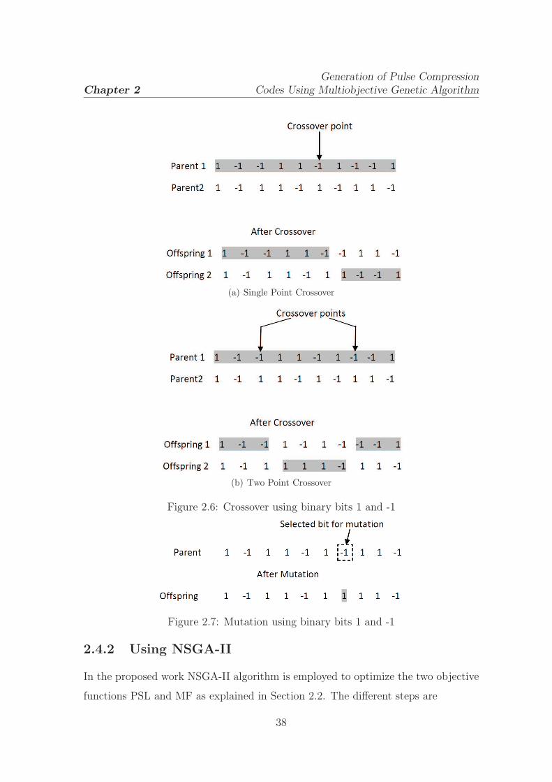
Chapter 2



(a) Single Point Crossover

(b) Two Point Crossover

Figure 2.6: Crossover using binary bits 1 and -1

Figure 2.7: Mutation using binary bits 1 and -1

2.4.2 Using NSGA-II

In the proposed work NSGA-II algorithm is employed to optimize the two objective

functions PSL and MF as explained in Section 2.2. The different steps are

38

Chapter 2



1. The population is initialized with random binary bits (1 or -1) as in case of

GA.

2. The two objective functions are evaluated as given in (2.3) and (2.4). PSL is

minimized and MF is maximized simultaneously using the NSGA-II algorithm.

3. The chromosomes are sorted according to nondominated sort and found out

all possible fronts as described in Section 2.3.2.

4. The crowding distance for chromosomes in each front are evaluated according

to the procedure explained in Section 2.3.2.

5. The chromosomes are selected using binary tournament selection according to

Section 2.3.2.

6. The selected chromosomes undergo genetic operations such as crossover and

mutation to produce off-springs as explained in case of GA.

7. The off-spring population is combined with parent population and the best M

chromosome selected for next generation as described in Section 2.3.2

The steps from 5 to 7 are carried out until the maximum number of generations is

met.

2.5 Simulation results

The GA dealt in Section 2.3.1 is used to maximize the fitness function f given in (2.5)

to obtain the desired binary string. The population size M is chosen as 250 for each

code generation. Each chromosome is randomly initialized and the fitness function

f is calculated for all the chromosomes for a given combination of α and β. The

process of selection, crossover and mutation are carried out to produce offspring. The

two point crossover is used to generate the offspring. The probability of crossover

and mutation are chosen to be 0.8 and 0.2 respectively. The current generation

population is mixed with the offspring population and the best M chromosomes are

39

Chapter 2



Table 2.1: Sequences obtained using GA

Seq Len α β PSL MF Sequences

49

0.9 0.1 5 3.5309 11010111001010101101101000011011001111111011001110.8 0.2 5 4.0557 10010011100101111000000010101000010000110010110010.7 0.3 6 4.2271 11000101110111001011101010011110011010000001001010.6 0.4 6 4.2875 01010110000111100111000000101111011101111101100110.5 0.5 6 4.6173 1111111100011010001110100010101101001100111100100

50

0.9 0.1 5 3.1807 110100001001000000101001011101011100000100110111000.8 0.2 5 3.6232 111011011000100100001010100010011110010000110011110.7 0.3 6 3.7994 100110000110010001100101010010100111110100000100000.6 0.4 6 3.8941 010101000101001011011101101100110001100011111000000.5 0.5 7 3.9936 10100011001100101001111010001111101111010100000110

51

0.9 0.1 5 3.6429 1000111001010110100011000000010111110001001001001000.8 0.2 6 3.6841 1011010001011000001001010000110101111100110011001110.7 0.3 6 3.7264 0010110111111101101001100101010100001101110000111100.6 0.4 6 3.7696 0101011000110001010101110000001111101110110110110100.5 0.5 7 3.9529 011100101110000010011100001001110111101101100101001

52

0.9 0.1 5 3.9075 11100111100110010000111110000000100100101010101011010.8 0.2 6 4.0479 10111110110010111111100001100001010010101100110011000.7 0.3 6 4.2516 00111111011000111000100100011111101011010011011101010.6 0.4 6 4.3057 10101010011100011101001001100111111000000001001000010.5 0.5 8 4.7943 1101011010000000010011110000111011100010111010011001

53

0.9 0.1 6 3.9075 100111111011000111011010110001110101111110100110100010.8 0.2 6 3.6767 001011011100111011101101011110000110000010111110101000.7 0.3 6 3.7553 010100101101101100000111100011000100011111101110111010.6 0.4 7 4.2561 110001101001011001011001100110000000011111010101111010.5 0.5 7 4.5306 01010100011000101111001101101100111101011011110100000

selected to carry out the next generation. The algorithm is run for 100 generations

for each code. For different combinations of α and β the obtained codes from 49

to 53 are tabulated in Table 2.1. 0’s are used in place of -1’s to conserve space.

From Table 2.1 it is observed that by giving different weightage to PSL and MF

different codes are obtained. A particular code is selected according the requirement

of application such as low PSL or high MF. If it requires low PSL, then a high value

of α is required. If it requires high MF, then a high value of β is required. It is

too difficult to choose the appropriate values for α and β to get an optimized code.

The combination α = 0.8 and β = 0.2 produces better code as compared to the

combination α = 0.9 and β = 0.1. Because in both the cases PSL is same but for

the weight combination α = 0.8 and β = 0.2 provides better MF.

40

Chapter 2



Table 2.2: Sequences obtained using NSGA-II

Seq Len PSL MF Sequences

494 4.2875 00111110001111110110000001001011001110011010101015 5.0869 00111111001111110110000001001011001101001010101016 5.1746 0011111100111111011010000100111100110100101010101

505 3.7994 000100100111001111001001010001101110101011111110106 3.8941 100100000111001111001001010001101110101011111110107 4.4484 10010000111100111100100101000110111010101111111010

515 4.3788 1100000100000001101001100111000100010111100101011016 5.1403 100010010000000110100110111100010001011110010101001

525 4.4768 00001100110011000011110000000010100010110101011011016 4.7943 0101001110001110100101110110110100000001101100010011

535 3.9675 110010011010010000000100010011101011110000101011100016 4.0129 11111011011101101000011100111001000010111010101100100

545 3.8880 0111101011010010001000001100001110101000100111011101006 3.9728 1101101011010010001000001100001110101000100111011100007 4.1538 010110101101001000100000110000111010100010011101110000

555 3.6446 10001111000100010111110010001101010111111101011010010016 3.6800 1001101100010001111110001000011101011111110101111001011

565 3.4087 001110001000110111000110100010000000100110110100001111016 4.0412 001110101000110111000110100010000000101110110100001001017 4.2609 00111010100011011100011010001000000010011011010000100101

575 3.1240 1100110101111101011101101011100001000100100001111110110006 4.1441 1101100101111101011101101011100011000100100001111110110007 4.6151 110110010111010101110100101110001100010010000101111011000

585 3.7798 10010100011101110001010111110000111010011101100100000000106 4.8195 1001010001110011000101011011000011101001110110010000000000

595 3.5020 000001001011000011111111000101011000111101000110010011101016 4.2555 000001011011010011111011000101011100111101000110110011101007 4.4288 00000100101101001111111100010101110011110100011001001110101

To overcome the difficulty of choosing the values of α and β and to get the

optimized code in a single run, the code is generated by using multiobjective

GA. PSL and MF are the two objective functions used for optimization using

NSGA-II algorithm as explained in Section 2.4.2. The population size M is taken

as 250 and the chromosomes are initialized randomly. The PSL and MF for each

chromosome are found out and the population is sorted based on nondomination.

Each chromosome in the first front have a rank value of 1 and the chromosome

in the second front is assigned a rank value of 2 and so on. Crowding distance is

assigned front wise to each chromosome. Parents are selected from the population

41

Chapter 2



using binary tournament selection based on rank and crowding distance. The

selected population generate offspring using crossover and mutation operations. The

probability of crossover and mutation are chosen same as earlier. In this case also two

point cross over is used to generate offspring. The offspring population is recombined

with the current population and the best M chromosomes are selected for next

generation. The number of generations is taken as 100. The sequences found by

the proposed method for length 49 to 59 are listed in Table 2.2. In this case all the

possible nondominated solutions can be achieved in a single run. For code length

49 the lowest PSL obtained is 4 and corresponding MF is 4.2875 which is better

the lowest PSL obtained using GA i.e. 5 and corresponding MF is 3.5309. For a

particular length, NSGA-II provides more than one solution. A solution is chosen

according to the requirement of the application such as better PSL or better MF.

2.6 Conclusion

By using NSGA-II algorithm a list of biphase sequences of length 49-59 has been

generated and is listed in Table 2.2 along with their PSL and MF values. The

results reveal that the proposed method performs better than the weighted sum

approach in GA. The search for optimum sequence depends on the selection of the

initial population of parent sequences. As the sequence length increases the search

procedure requires more time for obtaining a good solution. The quality of solution

improves with increase in the number of generations.

42

Chapter 3

Development and PerformanceEvaluation of New and EfficientANN Mismatch Filters forSidelobe Reduction

3.1 Introduction

The objective of pulse compression technique is to achieve appreciable PSR and

acceptable range sidelobes in an economical manner. The types of waveforms used

in this technique decide the cost and complexity of the radar system. The binary

phase codes have better range resolution as compared to frequency coded waveforms.

This advantage is obtained at the cost of high range sidelobes [27,28]. The reduction

or elimination of range sidelobes can be achieved in a pulse compression radar by

the use of a pulse which is coded in both amplitude and phase [29]. However, these

techniques are seldom used because of the expensive amplitude modulation circuitry.

With the increase in compactness and decrease in cost of the digital circuits due to

the revolution of very large scale integrated (VLSI) circuits, it is appropriate to

implement complex techniques offering improved performance. Therefore, efforts

were made to devise alternative methods which could provide acceptable range

sidelobes.

The range sidelobes of binary phase codes are reduced by using different types

43

Chapter 3

Development and Performance Evaluation of New and Efficient

ANN Mismatch Filters for Sidelobe Reduction

of digital filters whose parameters are determined by use of various algorithms. The

efficiency of different approaches are evaluated by the ISL, PSL, hardware complexity

involved and loss in SNR as compared to matched filter. Two methods are generally

used to suppress the sidelobes. First one employs an additional weighing network

after the matched filter. Rihaczek and Golden [30] have synthesized a filter in

frequency domain for 13-bit Barker code which is a simple network and is able to

suppress the sidelobes to an acceptable level. In this technique the complexity of

the digital processor is reduced due to presence of few tap weights in the tap-delay

filter. The second method is to design a mismatched filter directly [31, 32] instead

of placing a weighing filter after the matched filter. In [31], an optimum mismatch

filter is developed for 13-bit Barker code in least square (LS) sense, which gives

optimal performance in terms of ISL. The weights of this filter is designed in such

a way that the response which approximates (in least square sense) to a sequence,

has all its elements as zeros except for one non zero element present at the central

position. Zoraster [32] has used the linear programming (LP) to determine the filter

weights for reduction of the PSL of 13-bit Barker code. To achieve satisfactory peak

sidelobe and integrated sidelobes, the length of the LP filter should be very large

which effectively increases the hardware cost. Hua and Oksman [33] have combined

the advantages of [30] and [32] to obtain a new algorithm which provides lower peak

sidelobes for 13-bit Barker code. In this method the transfer function of the sidelobe

suppression filter is fitted with a polynomial expansion series in frequency domain,

which consists of some unknown expansion coefficients. By applying inverse Fourier

transform and LP, the coefficients of the transfer function can then be determined.

A mismatch filter in cascade with a finite impulse response (FIR) filter is used in [34]

to suppress the side lobes of Barker codes which requires less multipliers and adders

due to its symmetry.

With the advancement of adaptive signal processing and neural networks,

researchers have put their efforts to design the sidelobe reduction filters using these

techniques. Sidelobe reduction using adaptive filters are discussed in [35, 36] where

44

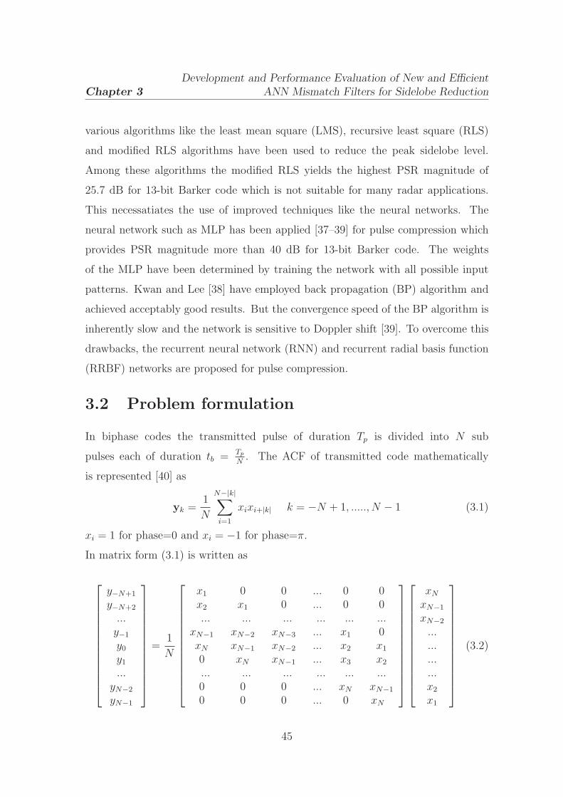
Chapter 3



various algorithms like the least mean square (LMS), recursive least square (RLS)

and modified RLS algorithms have been used to reduce the peak sidelobe level.

Among these algorithms the modified RLS yields the highest PSR magnitude of

25.7 dB for 13-bit Barker code which is not suitable for many radar applications.

This necessatiates the use of improved techniques like the neural networks. The

neural network such as MLP has been applied [37–39] for pulse compression which

provides PSR magnitude more than 40 dB for 13-bit Barker code. The weights

of the MLP have been determined by training the network with all possible input

patterns. Kwan and Lee [38] have employed back propagation (BP) algorithm and

achieved acceptably good results. But the convergence speed of the BP algorithm is

inherently slow and the network is sensitive to Doppler shift [39]. To overcome this

drawbacks, the recurrent neural network (RNN) and recurrent radial basis function

(RRBF) networks are proposed for pulse compression.

3.2 Problem formulation

In biphase codes the transmitted pulse of duration Tp is divided into N sub

pulses each of duration tb = Tp

N. The ACF of transmitted code mathematically

is represented [40] as

yk =1

N

N−|k|∑

i=1

xixi+|k| k = −N + 1, ....., N − 1 (3.1)

xi = 1 for phase=0 and xi = −1 for phase=π.

In matrix form (3.1) is written as

y−N+1

y−N+2

...y−1

y0

y1

...yN−2

yN−1

=1

N

x1 0 0 ... 0 0x2 x1 0 ... 0 0... ... ... ... ... ...

xN−1 xN−2 xN−3 ... x1 0xN xN−1 xN−2 ... x2 x1

0 xN xN−1 ... x3 x2

... ... ... ... ... ...0 0 0 ... xN xN−1

0 0 0 ... 0 xN

xN

xN−1

xN−2

...

...

...

...x2

x1

(3.2)

45

Chapter 3



The vector in the right hand side of (3.2) is the replica of the transmitted signal. In

other words they are the weighing sequence for the received signal. So (3.2) can be

expressed as

y =1

NXw1 (3.3)

where X is the matrix formed by shifting the input sequence {xi} and w1 is the

weight vector. It is observed from (3.2) that X has 2N − 1 number of patterns.

However, an additional null sequence {0} is considered for no input signal. So there

is 2N number of patterns that are used as the input to the pulse compression filter.

The desired output of the pulse compression filter for an input sequence is modeled

as a all zero vector except at one point at which the desired response is nonzero.

Thus the desired response is represented as

d = [0 0 0 . . . 1 0 0 0 . . .]T (3.4)

where [.]T denotes the transpose operation. The nonzero component represents the

mainlobe.

The problem is to design a suitable network for the pulse compression using input

output pairs so as to get better performance in terms of PSR for range resolution,

detection in presence of noise and Doppler shift. Different networks such as the

adaptive linear combiner (ALC), MLP, RNN, RBF and RRBF are used as pulse

compression network described in next section. The adaptive network contains

connecting weights which are trained by various learning algorithms such as the LMS,

RLS and BP etc. The weights of the filter, which provide input output relationship,

are determined in an iterative manner.

3.3 Techniques used

In this section various models such as ALC, MLP, RNN, RBF, RRBF and their

learning algorithms are discussed. These models are used as mismatch filter for

radar pulse compression.

46

Chapter 3



Figure 3.1: Adaptive linear combiner

3.3.1 Adaptive linear combiner

An ALC or nonrecursive adaptive filter is a computational device that attempts

to model the relationship between input and output in an iterative manner. The

general form of an ALC [42, 43] is depicted in Figure 3.1. The input signals to the

ALC are patterns and the nth pattern is represented as

x(n) = [x1(n), x2(n), .....xN (n)]T (3.5)

where N represents the number of elements in each pattern. The ALC contains a

set of adjustable weights given by

w = [w1, w2, .....wN ]T (3.6)

The estimated output of nth pattern is

y(n) = wTx(n) (3.7)

The training algorithms for ALC are explained below.

(a)Least mean square algorithm

There are many algorithms found in literature to train various adaptive models.

The performance of these algorithms depend on the rate of convergence, training

47

Chapter 3



time, computational complexity and residual mean square error (MSE). The LMS

algorithm is mostly used to train the weights of adaptive filters because of its low

computational complexity and ease of implementation. From Figure 3.1 the error

signal for nth pattern is obtained as

e(n) = d(n) − y(n) (3.8)

where d(n) is the desired output for nth pattern.

The cost function to be optimized is

ξ =1

2

n1∑

n=1

e2(n) (3.9)

where n1 is the number of patterns.

The weights associated with the filter are adjusted in such a way that the cost

function is minimized. The proposed study uses an epoch based adaptation for

weight updation. The ALC is trained with all n1 patterns and the change in weight

for each pattern is stored. These change in weights are used for a single update of

the filter weights which in turn constitutes an epoch. The new weights are used to

carry out the next epoch. The LMS algorithm uses the gradient descent technique

to minimize the cost function and the weights are updated [43] as

wk(m + 1) = wk(m) − µ∂ξ

∂wk(m)= wk(m) + µ

n1∑

n=1

e(n)x(n) (3.10)

where k = 1, 2....N and m is the epoch index.

(b)Recursive least square algorithm

The algorithm such as LMS is derived by using some approximation made in the

estimate of the performance function gradient. This type of algorithm have the

disadvantages that they are slow to obtain the optimum weight vector and once close

to it, usually “rattle around” the optimal vector rather than actually converging to

it. To overcome this difficulty, another efficient approach known as RLS algorithm

has been discussed in this section. The advantage gained by the use of the RLS

48

Chapter 3



algorithm is at the expense of an increase in computational complexity.

Steps involved in RLS algorithm

(a) Accept new pattern x(n) and corresponding desired output d(n).

(b) Compute the estimated output y(n) as expressed in (3.7). Initially assume the

weight vector as zero.

(c) Compute the error e(n) as given in (3.8).

(d) Compute filtered information vector z(n):

z(n) = R−1(m)x(n) (3.11)

where R is the autocorrelation matrix of input pattern. The R−1(m) is assumed

to be exist, where m is epoch index. Initially R−1(m) is taken as ηI, where I is

an identity matrix of size N × N . The value of η taken as very large i.e. about

104.

(e) Compute normalized error power q:

q = xT (n)z(n) (3.12)

(f) Compute gain constant v:

v =1

1 + q(3.13)

(g) Compute the normalized information vector z(n):

z = vz(n) (3.14)

(h) Compute the change in weight vector as

∆w(n) = e(n)z (3.15)

(i) Compute the change in inverse correlation matrix

∆R−1(n) = −z(n)zT (n) (3.16)

49

Chapter 3



The steps from (a) to (i) are carried out for all n1 patterns. The weights are updated

as

w(m + 1) = w(m) +

n1∑

n=1

∆w(n) (3.17)

and the inverse correlation matrix is updated as

R−1(m + 1) = R−1(m) +

n1∑

n=1

∆R−1(n) (3.18)

The updated values of the weights and the inverse correlation matrix are used to

carry out next epoch.

(c)Modified RLS algorithm

The modified RLS algorithm is derived by using the condition

|e(n)| ≥ Th (3.19)

where Th represents a threshold value. The instantaneous error is compared with

the threshold value. If the instantaneous error is greater than the threshold value

then steps from (d) to (i) of the RLS algorithm are evaluated otherwise not. If

|e(n)| < Th, then values of ∆R−1(n) and ∆w(n) are zero. The weights and the

inverse correlation matrix are updated as given in (3.17) and (3.18) respectively.

Initially the threshold value is chosen as very small and later it is updated for

each epoch based on the maximum error value at that epoch. The updation of

threshold at mth epoch is given by

maxerrm = maximum|em(n)| (3.20)

Thm= δ ∗ maxerrm (3.21)

where em(n) is the error vector at mth epoch and maxerrm is the maximum value of

all the errors in error vector. δ, a constant whose value is close or equal to 1, affects

the rate of convergence.

50

Chapter 3



3.3.2 Artificial neural network

An artificial neural network (ANN) is an information processing paradigm that

is inspired by the way biological nervous system, such as the brain, process

the information [44, 45]. The first artificial neuron was developed in 1943 by

the neurophysiologist Warren McCulloch and the logician Walter Pits. But the

technology available at that time did not allow them to proceed further. In

past few decades the ANN has emerged as a powerful learning tool to perform

complex tasks in highly nonlinear dynamic environment. The ANN is capable

of performing nonlinear mapping between the input and output space due to its

large parallel interconnection between different layers and the nonlinear processing

characteristic. Therefore, the ANN is used extensively in the field of communication,

control, instrumentation and forecasting [46–48]. ANN technique is also used for

classification, modeling and optimization problems [49,50].

An artificial neuron basically consists of a computing element that performs the

weighted sum of the input signal and the connecting weight. The sum is added with

the bias or threshold and the resultant signal is then passed through a nonlinear

function of sigmoid or hyperbolic tangent type. Each neuron is associated with

three parameters whose learning can be adjusted. These are the connecting weights,

the bias and the slope of the nonlinear function. For the structural point of view a

neural network (NN) may be single layer or it may be multilayer. In MLP there is a

number of layers and each layer contains one or many artificial neurons. Each neuron

of the one layer is connected to each and every neuron of the next layer. A trained

neural network can be thought of as an “expert” in the category of information it

has been given to analyze. The advantages of ANN are

(a) Adaptive learning: It is the ability of the network to learn how to do tasks

based on the data given for training or initial experience.

(b) Self-organization: An ANN can create its own organization or representation

of the information as it receives during learning time.

51

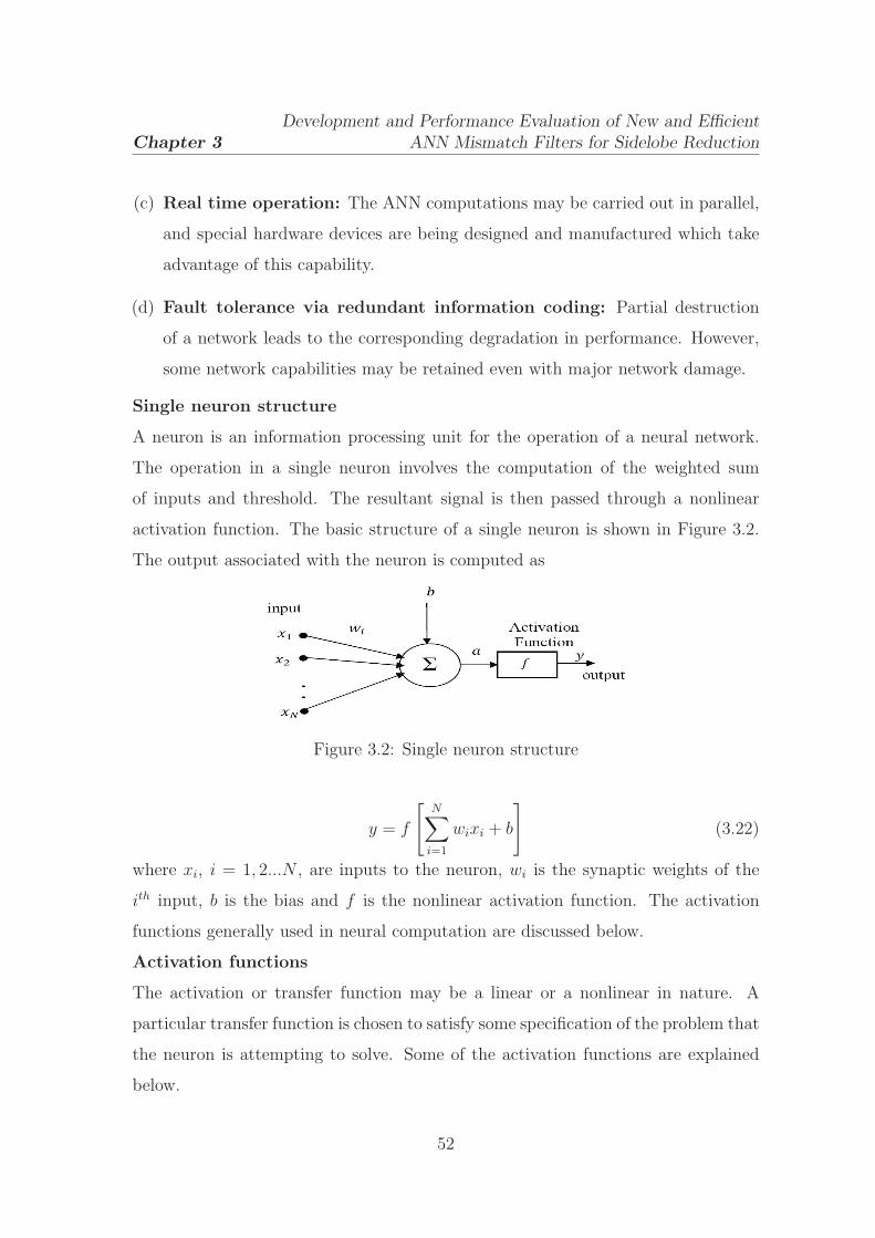
Chapter 3



(c) Real time operation: The ANN computations may be carried out in parallel,

and special hardware devices are being designed and manufactured which take

advantage of this capability.

(d) Fault tolerance via redundant information coding: Partial destruction

of a network leads to the corresponding degradation in performance. However,

some network capabilities may be retained even with major network damage.

Single neuron structure

A neuron is an information processing unit for the operation of a neural network.

The operation in a single neuron involves the computation of the weighted sum

of inputs and threshold. The resultant signal is then passed through a nonlinear

activation function. The basic structure of a single neuron is shown in Figure 3.2.

The output associated with the neuron is computed as

Figure 3.2: Single neuron structure

y = f

[

N∑

i=1

wixi + b

]

(3.22)

where xi, i = 1, 2...N , are inputs to the neuron, wi is the synaptic weights of the

ith input, b is the bias and f is the nonlinear activation function. The activation

functions generally used in neural computation are discussed below.

Activation functions

The activation or transfer function may be a linear or a nonlinear in nature. A

particular transfer function is chosen to satisfy some specification of the problem that

the neuron is attempting to solve. Some of the activation functions are explained

below.

52

Chapter 3



1. Log-sigmoid function

This transfer function takes the input and squashes the output into the range

of 0 to 1, according to expression given below

f(x) =1

1 + e−x(3.23)

2. Hyperbolic tangent Sigmoid:

This function is expressed as

f(x) = tanh(x) =ex − e−x

ex + e−x(3.24)

3. Signum Function:

The expression for this activation function is given by

f(x) =

1 if x > 0

0 if x = 0

−1 if x < 0

(3.25)

4. Threshold function

This function is given by the expression

f(x) =

1 if x ≥ 0

0 if x < 0(3.26)

5. Piecewise linear function

This function is represented as

f(x) =

1 if x > 0.5

x if − 0.5 ≤ x ≤ 0.5

0 if x < 0.5

(3.27)

53

Chapter 3



The different structures of neural network and their learning algorithms are described

below.

(i) Multilayer perceptron

The MLP is a feed forward network having an input layer, one or more hidden layer

and an output layer. The layer to which the input data is given called as input layer

and the layer from which output is taken called as output layer. All the intermediate

layers are called as hidden layers. The layers are fully interconnected i.e. each neuron

is connected to every neuron in previous and succeeding layers. The input signal

propagates through the network on a layer by layer basis. This network have been

applied successfully to solve many nonlinear and complex problems in several fields.

The structure of a three layer MLP is shown in Figure 3.3 which consists of input

layer, one hidden layer and output layer. i, j and k are the indices used for input,

hidden and output layer respectively. x(n) = [x1(n), x2(n), ..., xN (n)]T is the input

to the network for nth pattern and wji is the synaptic weight connecting input xi(n)

to the hidden neuron j. Similarly wkj is the synaptic weight connecting output of jth

hidden neuron output to the kth neuron of output layer. bj and bk are the biases to

the hidden layer and output layer respectively. f represents the nonlinear activation

function for both hidden and output layer. The activation functions can be different

for different layers. The output of jth hidden neuron for nth pattern is

yj(n) = f(aj(n)) (3.28)

where

aj(n) =

(

N∑

i=1

wjixi(n) + bj

)

(3.29)

The response of the kth output node is

yk(n) = f(ak(n)) (3.30)

where

ak(n) =

(

n2∑

j=1

wkjyj(n) + bk

)

(3.31)

54

Chapter 3



Figure 3.3: Mlutilayer perceptron network

and n2 is the number of hidden nodes.

Back propagation algorithm

This algorithm is used to train the parameters of the MLP to get optimum cost

function. Basically BP learning comprises of two passes through the different layers

of networks: a forward pass and a backward pass. In forward pass a pattern (input

vector) is applied to the input nodes and its effect propagates through the network

layer by layer. In forward pass the synaptic weights remain constant. On the

other hand during backward pass the synaptic weights and the biases are adjusted

according to the error correction rule. The parameters of the neural network are

updated by BP on epoch basis.

The error of the kth neuron output for nth pattern is

ek(n) = dk(n) − yk(n) (3.32)

where dk(n) and yk(n) are desired and estimated outputs respectively. The cost

55

Chapter 3



function which is to be minimized is defined as

ξ =1

2

n3∑

k=1

n1∑

n=1

ek(n)2 (3.33)

where n3 is the number of neurons in the output layer.

According to the gradient descent, each weight change in the network should be

proportional to the negative gradient of the cost function with respect to the specific

weights.

The local gradient for kth output neuron is

δk(n) = − ∂ξ

∂ek(n)

∂ek(n)

∂yk(n)

∂yk(n)

∂ak(n)= (dk(n) − yk(n)) f

′

(ak(n)) (3.34)

where f′

(ak(n)) is the first derivative of f(ak(n)) with respect to ak(n).

The local gradient for jth the hidden nodes is

δj(n) = −n3∑

k=1

∂ξ

∂ek(n)

∂ek(n)

∂yk(n)

∂yk(n)

∂ak(n)

∂ak(n)

∂yj(n)

∂yj(n)

∂aj(n)=

n3∑

k=1

δk(n)wkj(m)f′

(aj(n))

(3.35)

where m is the epoch index. The local gradients for all patterns are calculated in

each epoch. The change in weights for output layer in mth epoch is

∆wkj(m) = η1

n1∑

n=1

δk(n)yj(n) (3.36)

where η1 is the learning parameter. The change in biases for output layer is

∆bk(m) = η1

n1∑

n=1

δk(n) (3.37)

The output layer weights and biases are updated as

wkj(m + 1) = wkj(m) + ∆wkj(m) (3.38)

bk(m + 1) = bk(m) + ∆bk(m) (3.39)

The change in weights for hidden layer is

∆wji(m) = η1

n1∑

n=1

δj(n)xi(n) (3.40)

56

Chapter 3



The change in biases for hidden layer is

∆bj(m) = η1

n1∑

n=1

δj(n) (3.41)

The hidden layer weights and biases are updated as

wji(m + 1) = wji(m) + ∆wji(m) (3.42)

bj(m + 1) = bj(m) + ∆bj(m) (3.43)

(ii) Recurrent neural network

Recently, significant research work has been carried out to demonstrate the

effectiveness of recurrent neural network in modeling of nonlinear dynamic systems

[51–56]. The RNN has many advantages over static layered networks when used for

system identification and feed back controller [51,52]. Moreover, RNN is capable for

long range prediction in the presence of measurement noise and also able to filter the

noise from the inputs [57]. The RNNs are used to model the plant nonlinearities in

more efficient ways as compared to feed forward network. The RNN has at least one

feed back loop in its architecture which is not present in feed forward network. Thus

in the RNN, there may be one layer with feed back connections as well as there may

be neurons with self feed back where output of the neuron is fed back into itself as

the input. The presence of feed back loop affects heavily on the learning capability of

the network. Contrary to the MLP, the RNN is sensitive and adaptive to past inputs.

Among the several ANN architectures available in the literature, ANN having feed

back and internal dynamics have been considered more suitable for modeling and

control of the nonlinear systems as compared to feed forward network [58].

A block diagram of the RNN is shown in Figure 3.4. The RNN has structure as

that of MLP with feedback or recurrent connections. This network has recurrent

connections from the hidden neurons to a layer of context units consisting of bank

of unit delays [59]. These context units store the outputs of hidden neurons for one

time step and feed them back to the input layer. The inputs to the hidden layers

are combination of the present inputs and the outputs of the hidden layer which

57

Chapter 3



Figure 3.4: Block diagram of recurrent neural nerwork

are stored from previous time step in context layer. Hence the outputs of the RNN

are functions of present state, previous state (that is stored in context units) and

present inputs.

In this case the the jth hidden layer outputs are calculated as

yj(n) = f(aj(n)) (3.44)

where

aj(n) = f

(

N∑

i=1

wjixi(n) +

n2∑

h=1

ujhyj(n − 1) + bj

)

(3.45)

where n2 is the number of hidden nodes and ujh are the recurrent layer weights. The

response of the kth neuron in output layer is

yk(n) = f(ak(n)) (3.46)

where

ak(n) =

(

n2∑

j=1

wkjyj(n) + bk

)

(3.47)

Weight updation for recurrent neural network

The hidden node output is used to compute the response of output layer of the RNN

as given in (3.46). The local gradient and weight update procedure are same as that

of MLP. The change in recurrent layer weights are obtained as

∆uhj(m) = η1

n1∑

n=1

δj(n)yj(n − 1) (3.48)

Recurrent layer weights are updated as

uhj(m + 1) = uhj(m) + ∆uhj(m) (3.49)

58

Chapter 3



Hence all weights are updated based on the corresponding weight correction

equations.

(iii) Radial basis function network

The radial basis function network can be viewed as a feed forward neural network

with a single hidden layer which computes the distance between input pattern and

the center [60]. It consists of three layers, an input layer, a hidden layer and an

output layer. The input layer connects the network to the environment. The

second layer is the only hidden layer which transfer the input space nonlinearly

using radial basis function. The hidden space is greater than the input space in

most of the applications. The response of the network provided by the output

layer which is linear in nature. The RBF network is suitable for solving function

approximation, system identification and pattern classification because of its simple

topological structure and their ability to learn in an explicit manner [61, 62]. The

Figure 3.5: Architecture of radial basis function network

basic architecture of RBF network is shown in Figure 3.5. Here x(n) is the input to

the network and φ represents the radial basis function that perform the nonlinear

mapping and M represents the total number of hidden units. Each node has a center

vector ck and spread parameter σk, where k = 1, 2, ....M .

Radial basis functions

The radial basis functions are represented by φ(‖x, c‖), where ‖.‖ represents the

Euclidean norm. The radial basis functions which are generally used in various

59

Chapter 3



applications are

1. Multiquadratics

φ(r) = (r2 + c2)12 for c > 0, r ∈ R (3.50)

2. Inverse multiquadratics

φ(r) = (r2 + c2)−12 for c > 0, r ∈ R (3.51)

3. Gaussian function

φ(r) = exp(− r2

2σ2) for σ > 0, r ∈ R (3.52)

Learning algorithm for RBF network

The error for the nth pattern is obtained as

e(n) = d(n) −M∑

k=1

wk(m)φ (x(n), ck(m), σk(m))) (3.53)

where d(n) is the desired output. If the Gaussian function chosen as the radial basis

function

e(n) = d(n) −M∑

k=1

wk(m)exp

(

−‖x(n) − ck(m)‖2

σ2k(m)

)

(3.54)

The cost function is defined as

ξ =1

2

n1∑

n=1

e2(n) (3.55)

where n1 is the number of training patterns. It is required to adjust the free

parameters such as weight, center and spread so as to minimize ξ. According to

the gradient descent algorithm the free parameters for mth epoch are updated as

wk(m + 1) = wk(m) − µw∂ξ

∂wk(m)(3.56)

ck(m + 1) = ck(m) − µc∂ξ

∂ck(m)(3.57)

60

Chapter 3



σk(m + 1) = σk(m) − µσ∂ξ

∂σk(m)(3.58)

where µw, µc and µσ are learning parameters and k = 1, 2...M . Finally the updation

equations are defined as

wk(m + 1) = wk(m) +

n1∑

n=1

µwe(n)φ (x(n), ck(m), σk(m)) (3.59)

ck(m+1) = ck(m)+

n1∑

n=1

µce(n)wk(m)

σ2k(n)

φ (x(n), ck(m), σk(m)) [x(n)− ck(m)] (3.60)

σk(m + 1) = σk(m) +

n1∑

n=1

µσe(n)wk(m)

σ3k(m)

φ (x(n), ck(m), σk(m)) [‖x(n) − ck(m)‖2]

(3.61)

where

φ (x(n), ck(m), σk(m)) = exp

(

−‖x(n) − ck(m)‖2

σ2k(m)

)

(3.62)

(iv) Recurrent radial basis function

The RRBF [63] combines the advantages of RBF and dynamic representation of

time. The RRBF network has been applied for modeling [64], noise cancellation

[65, 66] and time series [67] prediction. This network has faster convergence [68]

while maintaining the modeling capability of neural networks. The architecture of

Figure 3.6: Architecture of recurrent radial basis function network

RRBF model is shown in Figure 3.6. The model of RRBF is similar to RBF with

an input layer, one hidden layer and an output layer. In this network each output of

61

Chapter 3



the hidden neurons are fed back to their corresponding input through a delay. The

estimated output of the network for nth pattern is

y(n) =M∑

k=1

wk(m)φ (x(n), ck(m), σk(m)) (3.63)

where

φ (x(n), ck(m), σk(m)) =

exp

(

−‖x(n) − ck(m)‖2

σ2k(m)

+ gk(m)φ (x(n − 1), ck(m), σk(m))

)

(3.64)

Learning algorithm for RRBF

In this case the cost function is same as that of RBF as defined in (3.55). wk, ck and

σk are updated as that of RBF using the currently defined φ (x(n), ck(m), σk(m)).

The recurrent weights are updated as

gk(m + 1) = gk(m) − µg∂ξ

∂gk(m)(3.65)

where µg is the learning parameter.

∂ξ

∂gk(m)=

n1∑

n=1

wk(m)φ (x(n), ck(m), σk(m)) φ (x(n − 1), ck(m), σk(m)) (3.66)

From (3.66) and (3.67)

gk(m + 1) =

gk(m) − µg

n1∑

n=1

wk(m)φ (x(n), ck(m), σk(m)) φ (x(n − 1), ck(m), σk(m)) (3.67)

where k = 1, 2...M .


This section illustrates the performance of various networks for radar pulse

compression. First, the performance of ALC trained with LMS, RLS and Modified

62

Chapter 3



RLS algorithm is presented. Subsequently the performances of MLP, RBF along

with the proposed RNN and RRBF are presented. All the networks are trained

with time shifted sequences of the 13-bit and 35-bit Barker codes. The time shifted

sequence for 13-bit Barker code is presented in Figure 3.7. A null sequence {0} is

added to the shifted sequence that represents radar has not received any information.

So there are 26 patterns for 13-bit Barker code. Similarly the number of patterns

in case of 35-bit Barker code is 70. In these training sequences the desired output

of the network is 1 when the proper Barker code present in the input, otherwise the

output is zero.

Figure 3.7: 26 different possible input sequences for 13-bit Barker codes

63

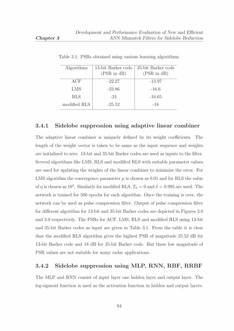
Chapter 3



Table 3.1: PSRs obtained using various learning algorithms.

Algorithms 13-bit Barker code 35-bit Barker code(PSR in dB) (PSR in dB)

ACF -22.27 -13.97

LMS -23.86 -16.6

RLS -24 -16.65

modified RLS -25.52 -18

3.4.1 Sidelobe suppression using adaptive linear combiner

The adaptive linear combiner is uniquely defined by its weight coefficients. The

length of the weight vector is taken to be same as the input sequence and weights

are initialized to zero. 13-bit and 35-bit Barker codes are used as inputs to the filter.

Several algorithms like LMS, RLS and modified RLS with suitable parameter values

are used for updating the weights of the linear combiner to minimize the error. For

LMS algorithm the convergence parameter µ is chosen as 0.01 and for RLS the value

of η is chosen as 104. Similarly for modified RLS, Th = 0 and δ = 0.995 are used. The

network is trained for 500 epochs for each algorithm. Once the training is over, the

network can be used as pulse compression filter. Output of pulse compression filter

for different algorithm for 13-bit and 35-bit Barker codes are depicted in Figures 3.8

and 3.9 respectively. The PSRs for ACF, LMS, RLS and modified RLS using 13-bit

and 35-bit Barker codes as input are given in Table 3.1. From the table it is clear

that the modified RLS algorithm gives the highest PSR of magnitude 25.52 dB for

13-bit Barker code and 18 dB for 35-bit Barker code. But these low magnitude of

PSR values are not suitable for many radar applications.

3.4.2 Sidelobe suppression using MLP, RNN, RBF, RRBF

The MLP and RNN consist of input layer one hidden layer and output layer. The

log-sigmoid function is used as the activation function in hidden and output layers.

64

Chapter 3



0 5 10 15 20 25−35

−30

−25

−20

−15

−10

−5

0

Time delay

Filte

r res

pons

e in

dB

(a)

0 5 10 15 20 25−35

−30

−25

−20

−15

−10

−5

0

Time delay

Filte

r res

pons

e in

dB

(b)

0 5 10 15 20 25−35

−30

−25

−20

−15

−10

−5

0

Time delay

Filte

r res

pons

e in

dB

(c)

0 5 10 15 20 25−35

−30

−25

−20

−15

−10

−5

0

Time delay

Filte

r res

pons

e in

dB

(d)

Figure 3.8: Filter response in dB for 13-bit Barker code obtained using (a)ACF(b)LMS (c)RLS (d)Modified RLS algorithms

65

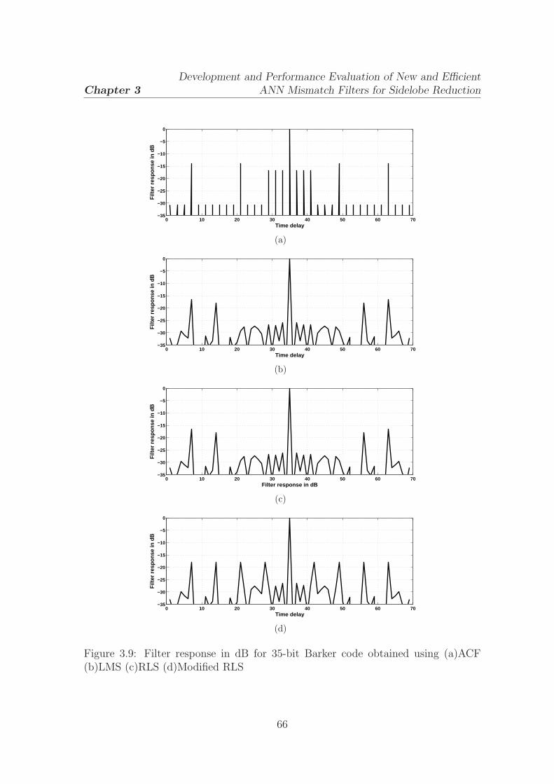
Chapter 3



0 10 20 30 40 50 60 70−35

−30

−25

−20

−15

−10

−5

0

Time delay

Filt

er r

espo

nse

in d

B

(a)

0 10 20 30 40 50 60 70−35

−30

−25

−20

−15

−10

−5

0

Time delay

Filt

er r

espo

nse

in d

B

(b)

0 10 20 30 40 50 60 70−35

−30

−25

−20

−15

−10

−5

0

Filter response in dB

Filt

er r

espo

nse

in d

B

(c)

0 10 20 30 40 50 60 70−35

−30

−25

−20

−15

−10

−5

0

Time delay

Filt

er r

espo

nse

in d

B

(d)

Figure 3.9: Filter response in dB for 35-bit Barker code obtained using (a)ACF(b)LMS (c)RLS (d)Modified RLS

66

Chapter 3



The number of input neurons are same as the length of the input code i.e. 13 for

13-bit Barker code and 35 for 35-bit Barker code. The number of hidden layer and

output layer neurons are chosen as three and one respectively. The weights and the

biases are randomly initialized. The learning parameter η1 is chosen as 0.8. The RBF

and RRBF consist of seven hidden neurons having Gaussian radial basis function

and one output neuron is used. Weight(w), centre(c) and spread (σ) parameters are

randomly initialized. The values of learning parameters µw, µc and µσ for RBF are

chosen as 0.75, 0.8 and 0.75 respectively. Similarly the values of learning parameters

µw, µc, µσ and µg for RRBF are chosen as 0.8, 0.8, 0.75 and 0.8 respectively. All the

four networks are trained for 500 epochs according to their learning algorithm given

in Section 3.3. After completion of the training, the neural network can be used for

pulse radar detection by using various set of input sequences.

Convergence performance

The MSE of all the networks for 13-bit and 35-bit Barker codes are depicted in

Figure 3.10. From the figure it is evident that the RRBF based approach offers

better convergence speed and very low residual error after training for 13-bit and

35-bit Barker codes as compared to all other networks.

PSR performance

After the training is over, different inputs are applied to the networks to examine

PSR performance. The compressed output of different networks for 13-bit Barker

code is shown in Figure 3.11. The PSR values of all the networks for 13-bit and

35-bit Barker codes are listed in Table 3.2. The table shows that the proposed

RRBF network have achieved highest PSR magnitude for both 13-bit and 35-bit

Barker codes compared to all other approaches.

Noise performance

Noise is a random signal which interferes with the target echoes. If the noise is

very high it may mask the target echo. So it is also required to examine the noise

67

Chapter 3



0 50 100 150 200 250 300 350 400 450 50010

−6

10−5

10−4

10−3

10−2

10−1

Epochs

Mea

n sq

uare

err

or(lo

g10)

MLPRNNRBFRRBF

(a)

0 50 100 150 200 250 300 350 400 450 50010

−6

10−5

10−4

10−3

10−2

10−1

Epochs

Mea

n sq

uare

err

or(lo

g10)

MLPRNNRBFRRBF

(b)

Figure 3.10: Convergence graphs of different structures for (a)13-bit (b)35-bitsBarker codes

Table 3.2: PSRs obtained by various structures

Structures 13-Bit Barker Code 35-Bit Barker Code(PSR in dB) (PSR in dB)

MLP -42.61 -40.87

RNN -45.75 -44.93

RBF -60.43 -56.42

RRBF -64.31 -62.35

68

Chapter 3



0 5 10 15 20 25 300

0.2

0.4

0.6

0.8

1

1.2

Time delay

Filt

er

resp

on

se

(a)

0 5 10 15 20 25 300

0.2

0.4

0.6

0.8

1

1.2

Time delay

Filt

er

resp

on

se

(b)

0 5 10 15 20 25 30−0.2

0

0.2

0.4

0.6

0.8

1

1.2

Time delay

Filt

er

resp

on

se

(c)

0 5 10 15 20 25 30−0.2

0

0.2

0.4

0.6

0.8

1

1.2

Time delay

Filt

er

resp

on

se

(d)

Figure 3.11: Compressed waveforms for 13 bit Barker code using (a)MLP (b)RNN(c)RBF (d)RRBF structures

69

Chapter 3



rejection ability of different networks. The inputs having different SNR ranging

from 0 dB to 20 dB are applied to the networks and the output PSR for 13-bit and

35-bit Barker codes are listed in Tables 3.3 and 3.4 respectively. These tables show

that as the SNR increases the magnitude of PSR also increases. The RRBF provides

highest magnitude of PSR in all SNR values compared to those obtained by all other

approaches.

Table 3.3: Comparison of PSRs in dB at different SNRs for 13-bit Barker code

Structures SNR=0dB SNR=5dB SNR=10dB SNR=15dB SNR=20dBMLP -14.23 -28.61 -36.71 -38.53 -39.82

RNN -17.11 -32.17 -38.35 -40.59 -41.76

RBF -35.28 -45.23 -50.33 -55.77 -57.62

RRBF -40.24 -49.27 -57.30 -60.12 -61.24

Table 3.4: Comparison of PSRs in dB at different SNRs for 35-bit Barker code

Structures SNR=0dB SNR=5dB SNR=10dB SNR=15dB SNR=20dBMLP -15.18 -29.17 -32.43 -36.95 -38.12

RNN -19.52 -32.74 -37.83 -40.87 -42.65

RBF -40.25 -48.25 -52.78 -54.44 -55.17

RRBF -42.25 -54.69 -57.47 -58.60 -60.57

Range resolution ability

The range resolution is to analyze the ability of a particular network to distinguish

between two targets by measurement of their ranges in the radar system. The two

targets which are to be resolved must be separated by at least the range equivalent

of the width of the processed echo. To compare the range resolution ability two

overlapping codes of same length are considered with n-delay apart (DA) having

70

Chapter 3



Table 3.5: Comparison of range resolution ability for 13-bit Barker code of twotargets having same IMR and DA.

Structures 2-DA 3-DA 4-DA 5-DA(PSR in dB) (PSR in dB) (PSR in dB) (PSR in dB)

MLP -36.53 -38.52 -37.32 -36.16

RNN -40.24 -41.23 -39.23 -38.78

RBF -53.32 -55.25 -56.76 -54.23

RRBF -59.72 -58.28 -60.73 -58.71

Table 3.6: Comparison of range resolution ability for 35-bit Barker code of twotargets having same IMR and DA.

Structures 2-DA 3-DA 4-DA 5-DA(PSR in dB) (PSR in dB) (PSR in dB) (PSR in dB)

MLP -34.41 -34.83 -33.75 -32.62

RNN -38.23 -37.79 -36.87 -35.25

RBF -48.34 -47.61 -49.82 -47.13

RRBF -53.72 -55.14 -54.25 -53.23

same or different input magnitude ratio (IMR). The IMR is defined as the magnitude

of first pulse train over that of the delayed pulse train. Figure 3.12 shows the added

input waveform of equal magnitude (IMR=1) with 5 delay apart for 13-bit Barker

code. The compressed output for this input for all the network are shown in Figure

3.13. In this case the PSR is calculated by taking lower value of the two mainlobes.

By varying the DA from 2 to 5 the PSR for 13-bit and 35-bit Barker codes are

obtained and shown in Tables 3.5 and 3.6 respectively. In Tables 3.7 and 3.8 the

PSR for different IMRs and DAs for all the networks are listed. From these tables

it is evident that the PSR values for RRBF are the best among those offered by

all other networks i.e. RRBF based pulse compression technique have best range

resolution ability compared to those of other networks.

71

Chapter 3



0 2 4 6 8 10 12 14 16 18 20−1

−0.8

−0.6

−0.4

−0.2

0

0.2

0.4

0.6

0.8

1

Time delay

Inp

ut

(a)

0 2 4 6 8 10 12 14 16 18 20−1

−0.8

−0.6

−0.4

−0.2

0

0.2

0.4

0.6

0.8

1

Time delay

Inp

ut

(b)

0 2 4 6 8 10 12 14 16 18 20−2

−1.5

−1

−0.5

0

0.5

1

1.5

2

Time delay

Ad

de

d in

pu

t

(c)

0 2 4 6 8 10 12 14 16 18 20−2

−1.5

−1

−0.5

0

0.5

1

1.5

2

Time delay

Inp

ut

(d)

Figure 3.12: Input waveform on addition of two 5-DA 13-bit Barker sequence havingsame magnitude (a)Left shift (b)Right shift (c)Added waveform (d)Waveform afterflip about the vertical axis

72

Chapter 3



0 5 10 15 20 25 300

0.2

0.4

0.6

0.8

1

1.2

Time delay

Filt

er

resp

on

se

(a)

0 5 10 15 20 25 300

0.2

0.4

0.6

0.8

1

1.2

Time delay

Filt

er

resp

on

se

(b)

0 5 10 15 20 25 30−0.2

0

0.2

0.4

0.6

0.8

1

1.2

Time delay

Filt

er

resp

on

se

(c)

0 5 10 15 20 25 30−0.2

0

0.2

0.4

0.6

0.8

1

1.2

Time delay

Filt

er

resp

on

se

(d)

Figure 3.13: Compressed waveforms for 13-bit Barker code having same IMR and 5DA for (a)MLP (b)RNN (c) RBF (d)RRBF structures

73

Chapter 3



Table 3.7: Comparison of range resolution ability for 13-bit Barker code of twotargets having different IMR and DA.

Structures 2-DA 3-DA 4-DA 5-DA2-IMR 3-IMR 4-IMR 5-IMR

(PSR in dB) (PSR in dB) (PSR in dB) (PSR in dB)MLP -38.17 -30.23 -24.16 -12.14

RNN -40.23 -36.56 -31.14 -23.65

RBF -51.38 -49.42 -43.24 -33.18

RRBF -56.36 -55.42 -50.24 -39.37

Table 3.8: Comparison of 35-bit Barker code for range resolution ability of twotargets having same IMR and DA

Algorithms 2-DA 3-DA 4-DA 5-DA2-IMR 3-IMR 4-IMR 5-IMR

(PSR in dB) (PSR in dB) (PSR in dB) (PSR in dB)MLP -34.46 -27.75 -21.78 -14.54

RNN -39.44 -33.23 -26.74 -20.68

RBF -47.77 -45.24 -38.21 -25.23

RRBF -52.64 -48.71 -43.41 -35.42

Table 3.9: Doppler shift performance

Structures 13-bit Barker code 35-bit Barker code(PSR in dB) (PSR in dB)

MLP -14.35 -28.34

RNN -30.93 -42.36

RBF -47.45 -46.42

RRBF -55.23 -56.34

74

Chapter 3



Doppler shift performance

The influence of Doppler shift should be accounted for evaluating the detection

performance for a moving target. The Doppler tolerance measures the Doppler

sensitivity of the pulse compression technique. The Doppler sensitivity is caused by

the shifting in phase of the individual elements of the code by the target Doppler.

In extreme case the phase shift across the code will be 180o, the last subpulse in

the received code is effectively inverted. For 13-bit Barker code at extreme case the

input will change from “1 1 1 1 1 -1 -1 1 1 -1 1 -1 1” to “-1 1 1 1 1 -1 -1 1 1 -1 1 -1

1”. For 13-bit and 35-bit Barker codes the extreme case Doppler shift PSR values

for different types of network are listed in Table 3.9. From this table it is observed

that the MLP has very low Doppler tolerance and RRBF produces the best PSR

value of -55.23 dB for 13-bit Barker code.

3.5 Conclusion

In this chapter recurrent networks such as RNN and RRBF are proposed for radar

pulse compression. The simulation results reveal that the performance of RRBF

based pulse compression is much better than MLP, RNN and RBF based pulse

compression techniques. The convergence rate of RRBF is higher than that of all

other networks and it has low training error. The RRBF approach provides better

PSR values in different adverse conditions such as noise and Doppler shift conditions.

The range resolution ability of RRBF network is much superior than MLP, RNN and

RBF networks. Although the algorithms are applied for 13-bit and 35-bit Barker

codes, they can also be used for any other biphase codes.

75

Chapter 4

Effective Sidelobe Suppression ofLFM and Polyphase Codes UsingConvolutional Windows

4.1 Introduction

The pulse compression techniques dealt in Chapter 3 are meant for biphase codes.

These codes are easily generated and the correlators for these codes are very simple.

But the compressed output of biphase codes are associated with the high time range

sidelobes and these codes are more prone to Doppler shift. The application of a

pulse compression technique depends on how efficiently it reduces the range sidelobes

associated with the compressed waveforms. The number of Barker codes available

are very less. Hence, these codes seriously suffer from security problem. Apart

from biphase codes, polyphase codes and frequency modulated codes are also used

in radar systems. PSL of frequency modulated pulse and polyphase codes are lower

than that of the biphase codes. The frequency modulated and polyphase codes are

more Doppler tolerant and have less range sidelobes compared to biphase codes.

Different windows those are available in the literature are used for reducing the

range sidelobes of the compressed output in case of LFM and polyphase codes.

In most of the practical radar systems LFM waveform is extensively used because

it is more Doppler tolerant than phase coded signals. The matched filter output of

a point target for an arbitrary pulse is the ACF which forms a Fourier transform

76

Chapter 4

Effective Sidelobe Suppression of

LFM and Polyphase Codes Using Convolutional Windows

pair with the energy spectrum of the signal. For rectangular amplitude weighing,

the energy spectrum of an LFM signal can be approximated as sin(x)/x or sinc(x)

shaped ACF. Hence a compressed LFM signal at the receiver will produce a series

of sidelobes surrounding the mainlobe and the first sidelobe occurs at a level of 13

dB below the peak of the mainlobe. Range sidelobes are inherent part of the pulse

compression mechanism and they occur due to abrupt rise in the signal spectrum.

The conventional method used to suppress these ambiguous sidelobes by modifying

the rectangular shape of the chirp spectrum using amplitude weighing. In radar

systems, weighing techniques in time or in the frequency domain are mostly employed

to reduce these range sidelobes with broadening in the mainlobe. Time domain

weighing is preferred to its frequency domain counterpart, as it produces lower peak

sidelobe in compressed output [69–71].

Although weighing when used both on transmitter and receiver provides better

results, weighing only on receiver is preferred. Weighing on transmitter leads to

power loss hence the available transmit power cannot be fully utilized. In low TB

product LFM waveforms the Fresnel ripples, which are responsible for producing

range sidelobes, are reduced by modifying the chirp waveform before transmission.

Amplitude tapering [69] and phase distortion [69, 72] are used to modify the chirp

waveform to suppress the peak sidelobe as well as to increase the fall off rate of far

sidelobes. Amplitude tapering reduces the far sidelobes effectively. But in most high

power radars, the control of the pulse rise time is very difficult. So an appropriate

phase distortion function is used in the LFM pulse for short rise time and high

power radars. Shennawy et. al. [73] have used an external Hamming window as

weighing function in frequency domain to suppress the range sidelobes from a TB

product of 50 to 720. Using the weighing technique the dynamic range of the pulse

compression system is increased. Hamming weighing has been used to suppress the

range sidelobes for rectangular LFM pulses with TB product less than 170 [74] and

it is observed from the results that Hamming weighing in time domain produces

lower peak sidelobe as compared to Hamming weighing in frequency domain. If

77

Chapter 4



weighing at the receiver is used, the reflected waveform from the object no longer

matched to the receiver filter which causes mismatch loss. In place of LFM, nonlinear

LFM (NLFM) can be used for transmission which does not need any weighing at

the receiver [75–77] to overcome the mismatch loss. If the objects are in motion

in the environment then the waveforms reflected are Doppler shifted version of the

transmitted signal and the matched filter output of these Doppler shifted signal

produces very low PSR magnitude. If the TB product of the transmitted signal

is low then the PSR magnitude becomes even worse. The NLFM signals are more

affected by Doppler shift and are difficult to design than the LFM signals.

Although LFM signal is popularly used in radar, the group of phase coded

pulses is also an active research area for particular radar applications. Phase

coded waveforms are more compatible for digital generation and compression [78].

However, these waveforms are affected more in the presence of Doppler shift as

compared to the LFM signal. To get the Doppler shift advantage of LFM signal

various polyphase codes are derived from LFM signal [79–81]. The codes such as

Frank [79], P1 and P2 [80] are derived from step approximation to LFM waveform.

These codes provide lower peak sidelobes than that offered by the best biphase

codes [10] for a particular length. In [81] two more polyphase codes, P3 and P4 are

discussed which are derived from the LFM signals. These codes are more Doppler

tolerant as compared to P1 and P2 codes. Although polyphase codes have lower

sidelobes in their ACF, it is required to further reduce the sidelobes for many

radar applications. Many sidelobe reduction techniques for polyphase codes such as

amplitude weighing [82,83] and the post compression sliding window techniques [84]

are found in the literature . When Doppler shift is zero these techniques substantially

reduce the sidelobes of the compressed pulse. Due to Doppler shift, objects with

larger velocities experience detection range degradation. Grating lobes are appeared

in the ACF of Frank and P1 code with increasing in Doppler shift [85]. Lee

and Griffiths [86, 87] have proposed Woo filter for polyphase codes which provides

optimum uniform sidelobe level and excellent Doppler shift performance. A modified

78

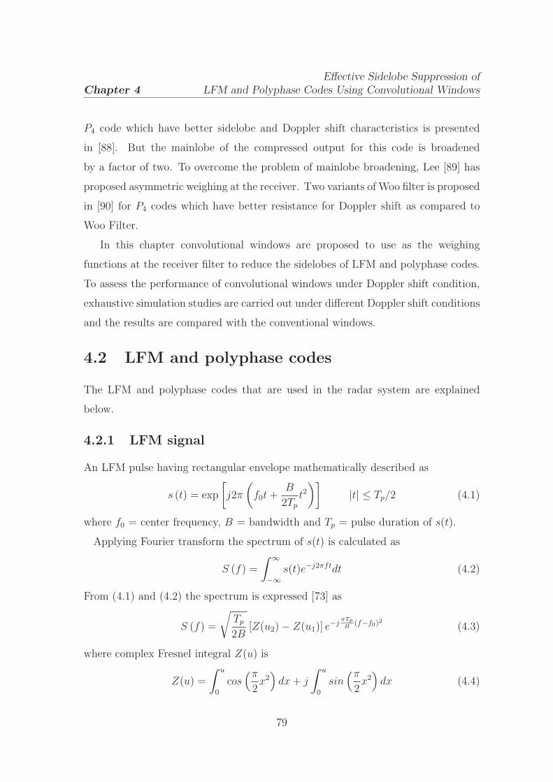
Chapter 4



P4 code which have better sidelobe and Doppler shift characteristics is presented

in [88]. But the mainlobe of the compressed output for this code is broadened

by a factor of two. To overcome the problem of mainlobe broadening, Lee [89] has

proposed asymmetric weighing at the receiver. Two variants of Woo filter is proposed

in [90] for P4 codes which have better resistance for Doppler shift as compared to

Woo Filter.

In this chapter convolutional windows are proposed to use as the weighing

functions at the receiver filter to reduce the sidelobes of LFM and polyphase codes.

To assess the performance of convolutional windows under Doppler shift condition,

exhaustive simulation studies are carried out under different Doppler shift conditions

and the results are compared with the conventional windows.

4.2 LFM and polyphase codes

The LFM and polyphase codes that are used in the radar system are explained

below.

4.2.1 LFM signal

An LFM pulse having rectangular envelope mathematically described as

s (t) = exp

[

j2π

(

f0t +B

2Tp

t2)]

|t| ≤ Tp/2 (4.1)

where f0 = center frequency, B = bandwidth and Tp = pulse duration of s(t).

Applying Fourier transform the spectrum of s(t) is calculated as

S (f) =

∫ ∞

−∞s(t)e−j2πftdt (4.2)

From (4.1) and (4.2) the spectrum is expressed [73] as

S (f) =

√

Tp

2B[Z(u2) − Z(u1)] e

−jπTp

B(f−f0)2 (4.3)

where complex Fresnel integral Z(u) is

Z(u) =

∫ u

0

cos(π

2x2)

dx + j

∫ u

0

sin(π

2x2)

dx (4.4)

79

Chapter 4



−5 −4 −3 −2 −1 0 1 2 3 4 5

−0.5

0

0.5

Time in µ sec

Real part of chirp signalA

mp

litu

de

−5 −4 −3 −2 −1 0 1 2 3 4 5

−0.5

0

0.5

1

Time in µ sec

Imaginary part of chirp signal

Am

plit

ud

e

Figure 4.1: Real and imaginary part of the chirp signal for TB = 50

The arguments u1 and u2 given by

u1 = −2(f − f0)

√

Tp

2B−√

TpB

2(4.5)

u2 = −2(f − f0)

√

Tp

2B+

√

TpB

2(4.6)

Z(u) is a function of Fresnel integrals cosine C(u) and sine S(u), where

C(u) =

∫ u

0

cos(π

2x2)

dx (4.7)

S(u) =

∫ u

0

sin(π

2x2)

dx (4.8)

The Fresnel ripple values defined in (4.7) and (4.8) are high at small arguments of u

and vice-versa. The real and imaginary part of the envelope of s(t) and corresponding

spectrum for TB = 50 are depicted in Figures 4.1 and 4.2 respectively. From Figure

4.2 it is observed that the spectrum contains the ripples called as Fresnel ripples,

which causes the sidelobes after compression. The output of the receiver matched

filter or compression filter for TB = 50 is a pulse with sin(x)x

envelope as shown in

Figure 4.3.

80

Chapter 4



−10 −8 −6 −4 −2 0 2 4 6 8 10

10

20

30

40

50

60

70

80

Frequency in MHz

Am

plitu

de

Figure 4.2: Amplitude spectrum of chirp signal for TB = 50

−1 −0.8 −0.6 −0.4 −0.2 0 0.2 0.4 0.6 0.8 1−50

−40

−30

−20

−10

0

Time delay × Tp

Filt

er r

espo

nse

in d

B

Figure 4.3: Compressed envelope

4.2.2 Polyphase codes

The complex envelope of phase coded pulse is expressed as [5]

u(t) =1√

Tp

N∑

i=1

uirect

[

t − (i − 1)tbtb

]

(4.9)

where rect(

ttb

)

= 1 for |t| ≤ tb2, ui = exp(jφi), tb is the sub pulse width and N is

the number of phases given as {φ1, φ2..., φN}.Polyphase codes have harmonically related phases based on a certain fundamental

phase increments. These codes have better Doppler tolerance and sidelobe

performance than biphase codes. These codes are discrete time sequences having

constant magnitude with a variable phase φi. Polyphase codes have more than

two elements or phase values. Increasing the number of elements in the sequence

enables construction of longer sequences having greater range resolution with a

larger compression ratio. But the trade off is that a more complex matched filter as

81

Chapter 4



compared to the biphase codes. These codes are derived by detecting a frequency

modulated pulse compression waveform with either a local oscillator at the band

edge of the waveform (single sideband detection) or at band center (double sideband

detection) and the resultant in phase I and quadrature phase Q data are sampled

at Nyquist rate.

Polyphase codes are derived from step approximation to linear frequency

modulation, such as Frank, P1 and P2 or from linear frequency modulation like

P3 and P4 codes.

(a)Frank Code

The Frank code is derived from step approximation to a linear frequency modulated

waveform having N frequency steps and N samples per frequency [79]. So Frank

code having N frequency steps have length Nc = N2. The first N samples of the

code have zero phase. The second N samples start with zero phase and increase

with a phase value of 2π/N from sample to sample. The phase of ith sample of jth

frequency step is given by

φi,j =2π

N(i − 1)(j − 1) (4.10)

where i = 1, 2, 3...N and j = 1, 2, 3...N .

The Frank code in N × N matrix form is given as

0 0 0 ... 0

0 1 2 ... N − 1

0 2 4 ... 2(N − 1)

... ... ... ... ...

0 N − 1 2(N − 1) ... (N − 1)2

(4.11)

where the number in matrix represent the multiplying coefficient with the phase

angle 2π/N . The Frank polyphase code is formed by concatenating the rows of the

Frank matrix and multiplying by fundamental phase increment 2π/N .

The 16-element Frank code is given by

82

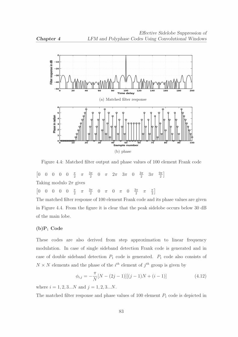
Chapter 4



0 20 40 60 80 100 120 140 160 180 200−50

−40

−30

−20

−10

0

Time delay

Filte

r res

pons

e in

dB

(a) Matched filter response

0 10 20 30 40 50 60 70 80 90 1000

1

2

3

4

5

6

Sample number

Phas

e in

radia

n

(b) phase

Figure 4.4: Matched filter output and phase values of 100 element Frank code

[

0 0 0 0 0 π2

π 3π2

0 π 2π 3π 0 3π2

3π 9π2

]

Taking modulo 2π gives[

0 0 0 0 0 π2

π 3π2

0 π 0 π 0 3π2

π π2

]

The matched filter response of 100 element Frank code and its phase values are given

in Figure 4.4. From the figure it is clear that the peak sidelobe occurs below 30 dB

of the main lobe.

(b)P1 Code

These codes are also derived from step approximation to linear frequency

modulation. In case of single sideband detection Frank code is generated and in

case of double sideband detection P1 code is generated. P1 code also consists of

N × N elements and the phase of the ith element of jth group is given by

φi,j = − π

N[N − (2j − 1)][(j − 1)N + (i − 1)] (4.12)

where i = 1, 2, 3...N and j = 1, 2, 3...N .

The matched filter response and phase values of 100 element P1 code is depicted in

83

Chapter 4



0 20 40 60 80 100 120 140 160 180 200−50

−40

−30

−20

−10

0

Time delay

Filte

r res

pons

e in

dB


0 10 20 30 40 50 60 70 80 90 1000

1

2

3

4

5

6

7

Sample number

Phas

e in

radia

n

(b) phase

Figure 4.5: Matched filter output and phase values of 100 element P1 code

Figure 4.5. From Figures 4.4(a) and 4.5(a) it is observed that the ACFs of Frank

and P1 codes are same. But the difference between P1 code and the Frank code is

that P1 code has the highest phase increments from sample to sample at the two

ends of the code but the Frank code has the highest phase increments from sample

to sample in the center of the code. So when the codes are passed through band

pass amplifier of a radar receiver, the P1 code is attenuated mostly at the two ends

of the waveform while the Frank code is attenuated most heavily in the center of

the waveform.

(c)P2 Code

In P2 code the starting phases are different from P1 code but the phase increments

within each phase group is same as that of P1 codes. The phases of P2 codes of

length N2 is given by

φi,j =π

2N[N − 1] − π

N(i − j)[N + 1 − 2j] (4.13)

84

Chapter 4



where i = 1, 2, 3...N and j = 1, 2, 3...N .

The matched filter response and phase value of 100 element P2 code is shown in

Figure 4.6. It has same matched filter output as that of Frank and P1 codes. But,

the P1 and P2 codes are more precompression bandwidth limit tolerant than the

Frank code.

0 20 40 60 80 100 120 140 160 180 200−50

−40

−30

−20

−10

0

Time delay

Filte

r res

pons

e in

dB


0 10 20 30 40 50 60 70 80 90 1000

1

2

3

4

5

6

7

Sample number

Phas

e in

radia

n

(b) phase


(d)P3 Codes

P3 codes [81] are derived from the phase samples LFM signal. These codes are

obtained by converting a LFM waveform to base band using a local oscillator on

one end of the frequency sweep (single sideband detection) and sampling the I and

Q video at Nyquist rate.

Let the waveform have pulse duration Tp and the instantaneous frequency is

f(t) = f0 + kt (4.14)

85

Chapter 4



where k is a constant and defined as

k =B

Tp

(4.15)

B is the bandwidth of the signal. So the signal will support a compressed pulse

length of

tc = 1/B (4.16)

The pulse compression ratio is obtained as

ρ = Tp/tc = BTp (4.17)

If the first samples of I and Q are taken at the leading edge of the waveform, the

phases of P3 codes are given by

φi = 2π

∫ (i−1)tc

0

[(f0 + kt) − f0]dt = πk(i − 1)2t2c (4.18)

From (4.17) and (4.18)

φi = π(i − 1)2/BTp = π(i − 1)2/ρ (4.19)

The matched filter output and phase values of 100 element P3 code are shown in

Figure 4.7. From Figure 4.7(a) it is observed that the peak side lobe occurs below

27 dB from the main peak lobe which is 3 dB inferior from the Frank code.

(e)P4 Codes

The P4 code is derived from the same waveform as P3 codes but the local oscillator

frequency is set at f0 + kTp/2. So the phase of P4 codes are

φi = 2π

∫ (i−1)tc

0

[(f0 + kt) − (f0 + kTp/2)]dt = [π(i − 1)2/ρ] − π(i − 1) (4.20)

The matched filter output and phase values of 100 element P4 code is shown in

Figure 4.8. From Figures 4.7(a) and 4.8(a) it is observed that both P3 and P4 codes

have the same matched filter output. But P4 code is more tolerant to precompression

bandwidth limitation as compared to P3 code.

86

Chapter 4



0 20 40 60 80 100 120 140 160 180−50

−40

−30

−20

−10

0

Time delay

Filter

resp

onse

in dB


0 10 20 30 40 50 60 70 80 90 1000

1

2

3

4

5

6

7

Sample number

Phas

e ang

le

(b) phase


0 20 40 60 80 100 120 140 160 180 200−50

−40

−30

−20

−10

0

Time delay

Filte

r res

pons

e in

dB


0 10 20 30 40 50 60 70 80 90 1000

1

2

3

4

5

6

7

Sample Number

Phas

e an

gle

(b) phase


87

Chapter 4




The LFM signal and polyphase codes are used for transmission and the reflected

waveforms are passed through weighted matched filter. If the target is in motion

the reflected waveform is Doppler shifted version of the transmitted waveform. The

Doppler shifted waveform is passed through the weighted receiver matched filter and

PSRs are calculated for different Doppler shift conditions.

4.3.1 For LFM signal

The matched filter is given by

H(f) = F [s(t)w(t]∗ (4.21)

where w(t) is the window function. The matched filter output is obtained as

g(t) = F−1[S(f)H(f ] (4.22)

where S(f) = F [s(t)].

The Doppler shifted version of the transmitted signal s(t) is represented as

sd (t) = exp

[

j2π

(

(f0 + fd)t +B

2Tp

t2)]

|t| ≤ Tp/2 (4.23)

where fd is the Doppler shift. The Doppler shifted signal is passed through the

weighted matched filter and the PSR values under different Doppler shift are

obtained. To achieve higher magnitude of PSR the transmitted signal is modified

using amplitude tapering and phase predistortion function as explained below

(I) Amplitude tapering: The Fresnel ripples can be reduced by adding cosine

taper of length αTp to the LFM pulse. The amplitude tapered transmitted

signal is represented as

s1 (t) = gT (t) exp{

j2π(

f0t + B2Tp

t2)}

|t| ≤ (0.5 + α) Tp (4.24)

88

Chapter 4



where

gT (t) =

1 |t| ≤ Tp/2

0.5{

1 + cos(

π |t|−Tp/2

αTp

)}

Tp/2 ≤ |t| ≤ (0.5 + α) Tp

0 elsewhere

(4.25)

and α is a parameter.

(II) Phase distortion: In high power pulsed radars the pulse rise time cannot be

controlled easily. So an alternate approach which uses an appropriate phase

distortion of the transmitted LFM signal is used for fast rise time transmitters.

LFM waveform having cubic phase distortion is given by

s2(t) = exp[

j2π{

f0t + B2Tp

t2 + φ(t)}]

|t| ≤ Tp/2 + ∆T (4.26)

where

φ (t) =

∆B3∆T 2 (−t − Tp/2)3 − Tp/2 − ∆T ≤ t < −Tp/2

∆B3∆T 2 (t − Tp/2)3 Tp/2 ≤ t < Tp/2 + ∆T

0 elsewhere

(4.27)

and ∆B and ∆T are the parameters.

4.3.2 For polyphase codes

These codes have discrete values having different phases. The matched filter is

designed according to the transmitted polyphase code. The filter is multiplied with

the window functions to achieve lower sidelobes. The Doppler shifted signal is

modeled by multiplying ej2πifd/B to the transmitted signal, where i = 1, 2, 3...N

and N is the code length.

The PSR values are calculated using conventional and convolutional windows as

weighing function at the receiver end under various Doppler shift conditions.

89

Chapter 4



4.4 Windows used for sidelobe suppression

Windows are time domain weighing functions that are used to reduce Gibbs

oscillations caused by the truncation of a Fourier series. They are employed in a

variety of traditional applications including power spectral estimation, beam forming

and digital filter design [91]. Many windows appeared in the literature are not

optimal. So the use of a particular window depends upon the application. A number

of windows and algorithms are formulated to find an optimal window for a given

application [92–96]. The typical windows that are used in the signal processing

techniques are based on cosine series such as Hamming, Hanning and Blackman [92].

Although many windows have already been introduced in the literature, research is

going on to propose new windows or to parameterize the known windows [97–100].

Window functions are generally categorized as fixed or adjustable. Fixed windows

have window length as the parameter which alters the mainlobe width. Adjustable

windows have two parameters, namely the window length and a parameter that

alters the relative sidelobe amplitude. The best known parametric windows in

the literature are Dolph-Chebysev [101] and Kaiser [102] windows. By varying the

two adjusting parameters of the Kaiser window it can control the mainlobe width

and ripple ratio of the spectrum. Polynomial windows having low computational

complexity is presented in [103]. The frequency response of these windows can

easily be changed by modifying their coefficients in the time domain. Avci and

Nacaroglu [104] have proposed a new class of cosine hyperbolic windows having

low computational complexity due to power series expansion in its time domain

representation.

Convolutional windows are derived by convolving the window with itself.

Reljin et. al. [105] have discussed a class of windows that are generated by the

time convolution of classical windows to obtain both flat top and high sidelobe

attenuation. These windows are suitable for harmonic amplitude evaluation in

nonsynchronous sampling case. The convolutional windows from second to eighth

order for rectangular window are derived in [106]. These windows are applied for

90

Chapter 4



high accuracy harmonic analysis and parameter estimation of periodic signals. Phase

difference algorithm based on Nuttal self-convolutional window is used to eliminate

the measurement errors of dielectric loss factor [107]. Dielectric loss factor is caused

by non-synchronised sampling and non-integral periodic truncation conditions. A

self convolution Hanning window used for complex signal harmonics parameter

estimation has been presented in [108]. The convolutional window based phase

correction algorithm suppresses the impact of fundamental frequency fluctuation

and white noise on harmonic estimation. In this chapter convolutional windows are

used for weighing purpose to reduce the range sidelobes that are present in output

of pulse compression filter.

The windows employed for the analysis are

(i) Hamming window:

w(n) = 0.54 − 0.46 cos

(

2πn

N − 1

)

(4.28)

where n = 0, 1, ........(N − 1)

(ii) Hanning window:

w(n) = 0.5 − 0.5 cos

(

2πn

N − 1

)

(4.29)

(iii) Kaiser window:

w(n) =I0

(

β√

1 − ( 2nN−1

)2)

I0 (β)(4.30)

where I0 is the zeroth order modified Bessel function of the first kind and β is

a parameter determines the shape of the window.

(iv) Chebysev window: The Dolph-Chebyshev window is in the frequency domain

is represented as

W (k) = (−1)k cos[Ncos−1[β1cos(πkN

)]]

cosh[Ncosh−1(β1)](4.31)

where β1 = cosh[ 1N

cosh−1(10α1)] and α1 determines the level of the sidelobe

attenuation. The sidelobe level σ(dB) = 20α1. The Dolph-Chebyshev window

91

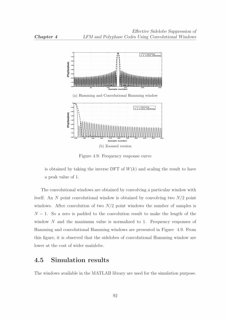
Chapter 4



50 100 150 200 250−80

−70

−60

−50

−40

−30

−20

−10

0

Sample number

20*lo

g10(a

mplitu

de)

HammingConv. Hamming

(a) Hamming and Convolutional Hamming window

130 140 150 160 170 180 190 200 210 220 230−80

−70

−60

−50

−40

−30

−20

−10

0

Sample number

20*lo

g10(a

mplitu

de)


(b) Zoomed version

Figure 4.9: Frequency response curve

is obtained by taking the inverse DFT of W (k) and scaling the result to have

a peak value of 1.

The convolutional windows are obtained by convolving a particular window with

itself. An N point convolutional window is obtained by convolving two N/2 point

windows. After convolution of two N/2 point windows the number of samples is

N − 1. So a zero is padded to the convolution result to make the length of the

window N and the maximum value is normalized to 1. Frequency responses of

Hamming and convolutional Hamming windows are presented in Figure 4.9. From

this figure, it is observed that the sidelobes of convolutional Hamming window are

lower at the cost of wider mainlobe.


The windows available in the MATLAB library are used for the simulation purpose.

92

Chapter 4



−1 −0.8 −0.6 −0.4 −0.2 0 0.2 0.4 0.6 0.8 1−50

−40

−30

−20

−10

0

Time delay × Tp

Filte

r res

pons

e in

dB

Figure 4.10: Matched filter output with Hamming weighing at the receiver

4.5.1 Analysis for LFM signals

LFM signal with low TB products is associated with Fresnel ripples. The compressed

output of an LFM signal having Hamming weighing at the receiver for TB = 50

is shown in Figure 4.10. The peak sidelobe is approximately 37 dB lower than

the main peak. The outputs of matched filter for different Doppler shifts using

Hamming and convolutional Hamming window are depicted in Figure 4.11. It

is observed that at zero Doppler shift Hamming window yields better PSR value

as compared to convolutional window. As the Doppler shift increases sidelobe

level affected very less in case of convolutional Hamming window as compared to

Hamming window. The PSR values under different Doppler shifts using various

windows are presented in Table 4.1. It is observed from the table that at lower

Doppler shift the conventional windows yield better PSR values as compared to

corresponding convolutional windows. On the other hand for higher Doppler shifts

the convolutional windows provide better PSR values than conventional ones. As

an illustration for fd

B= 0.01 the PSR for Hamming window is -36.2 dB and that of

convolutional Hamming window is -34.46. But, for fd

B= 0.2 the PSR for Hamming

window is -22.2 dB and that of convolutional Hamming window is -29 dB. From

Figure 4.11 it is obvious that the mainlobe width in case of convolutional window

is wider and the sidelobes near |t| = Tp

2region are not diminished by weighing

93

Chapter 4



−1 −0.8 −0.6 −0.4 −0.2 0 0.2 0.4 0.6 0.8 1−50

−40

−30

−20

−10

0

Time delay ×Tp

Filte

r res

pons

e in

dB


(a) fd

B= 0

−1 −0.8 −0.6 −0.4 −0.2 0 0.2 0.4 0.6 0.8 1−50

−40

−30

−20

−10

0

Time delay ×Tp

Filte

r res

pons

e in

dB


(b) fd

B= 0.05

−1 −0.8 −0.6 −0.4 −0.2 0 0.2 0.4 0.6 0.8 1−50

−40

−30

−20

−10

0

Time delay ×Tp

Filte

r res

pons

e in

dB


(c) fd

B= 0.1

Figure 4.11: Effect on sidelobes due to Doppler shift

94

Chapter 4



Table 4.1: Comparison of PSR for different Doppler shift for TB = 50

Doppler PSR using Hamming PSR using convolutional

Shift(fd

B) window in dB Hamming window in dB

0.01 -36.2 -34.460.05 -32.8 -33.670.1 -28.6 -32.50.15 -25.2 -310.2 -22.2 -29

Doppler PSR using Hanning PSR using convolutional

Shift(fd

B) window in dB Hanning window in dB

0.01 -31.68 -33.670.05 -30.32 -330.1 -27.62 -31.790.15 -24.47 -30.440.2 -22 -28.7

Doppler PSR using Kaiser PSR using convolutional

Shift (fd

B) window in dB (β = 6) Kaiser window in dB

0.01 -36.6 -34.20.05 -33 -33.40.1 -28.7 -32.260.15 -25.2 -30.860.2 -22.3 -29

Doppler PSR using Chebysev PSR using convolutional

Shift(fd

B) window in dB (σ = 50) Chebysev window in dB

0.01 -36 -34.30.05 -34.89 -33.50.1 -29.89 -32.50.15 -26.86 -310.2 -23.86 -29

technique. Hence to reduce the sidelobes at Tp

2region as well as peak sidelobe,

amplitude tapering and phase predistortion are used .

Amplitude tapering with α = 0.1 is used to modify the transmitter signal. In

simulation study the amplitude tapers are not used in compression filter. The

filter responses for amplitude tapering using Hamming and convolutional Hamming

95

Chapter 4



windows are depicted in Figure 4.12. From Figure 4.12(a), it is clear that amplitude

tapering reduces drastically the sidelobes around |t| = Tp/2 region but the reduction

of near in sidelobes is very less. From Figure 4.11, it is evident that the compressed

output of convolutional Hamming window produces peak sidelobe around |t| = Tp/2

region. So to get very low overall sidelobe the transmitted signal is amplitude tapered

and the receiver is weighed with convolutional Hamming window. The output

of pulse compression filter using convolutional Hamming window with amplitude

tapered transmitted signal is presented in Figure 4.12(b). The PSR values using

Hamming, Kaiser, convolutional Hamming and convolutional Kaiser windows for

TB = 50 and TB = 100 for different Doppler shifts are listed in Table 4.2. From

the table, it is observed that for higher TB product the PSR value is better and

amplitude tapering with convolutional window provides better PSR value compared

to that of conventional windows.

Table 4.2: PSR using amplitude tapering

Doppler Hamming Convolutional Hamming Kaiser Convolutional KaiserShift window window window (β = 6) window(

fd

B

)

PSR in dB PSR in dB PSR in dB PSR in dB

TB=50 TB=100 TB=50 TB=100 TB=50 TB=100 TB=50 TB=1000 -42.2 -43 -60 -78.7 -43.4 -44.5 -61.2 -79.6

0.02 -41.2 -42.7 -58 -75 -41.8 -43.8 -59.4 -78.20.04 -39 -41.7 -55.5 -71.4 -40 -42.5 -56.6 -75.50.06 -36.6 -39.3 -53 -67.3 -38.25 -40.8 -54 -71.380.08 -34.5 -36.8 -50.2 -63.5 -36.6 -39 -51.2 -66.80.1 -32.6 -34.7 -47.7 -60 -35 -37.3 -48.6 -62.70.12 -30.8 -32.7 -45.3 -55.7 -33.3 -35.7 -46.1 -58.50.14 -29.2 -31 -43 -52 -31.2 -33.4 -43.75 -54.50.16 -27.8 -29.4 -40.5 -48 -29.3 -31.2 -41.3 -50.70.18 -26.4 -28 -38.1 -44.4 -27.6 -29.8 -39 -46.80.2 -25.2 -26.5 -35.7 -41.2 -26 -28 -36.5 -43.3

In case of cubic phase distorted transmitted signal the parameter values used are

∆B = 0.75B and ∆T = 1/B. The filter responses for cubic phase distortion using

Hamming and convolutional Hamming windows are depicted in Figure 4.13. From

96

Chapter 4



−1 −0.8 −0.6 −0.4 −0.2 0 0.2 0.4 0.6 0.8 1

−80

−60

−40

−20

0

Time delay × Tp

Filte

r res

pons

e in

dB

(a) Compressed waveform for amplitude tapering with Hamming window

−1 −0.8 −0.6 −0.4 −0.2 0 0.2 0.4 0.6 0.8 1

−80

−60

−40

−20

0

Time delay × Tp

Filte

r res

pons

e in

dB

(b) Compressed waveform for amplitude tapering with convolutional Hamming window

Figure 4.12: Compressed waveforms for TB = 50 for amplitude tapering (α = 0.1)

−1 −0.8 −0.6 −0.4 −0.2 0 0.2 0.4 0.6 0.8 1

−80

−60

−40

−20

0

Time delay × Tp

Filte

r res

pons

e in

dB

(a) Compressed waveform for cubic phase distortion with Hamming window

−1 −0.8 −0.6 −0.4 −0.2 0 0.2 0.4 0.6 0.8 1

−80

−60

−40

−20

0

Time delay × Tp

Filte

r res

pons

e in

dB

(b) Compressed waveform for cubic phase distortion with convolutional Hamming window

Figure 4.13: Compressed waveforms for TB = 50 for cubic phase distortion (∆B =0.75B and ∆T = 1

B)

97

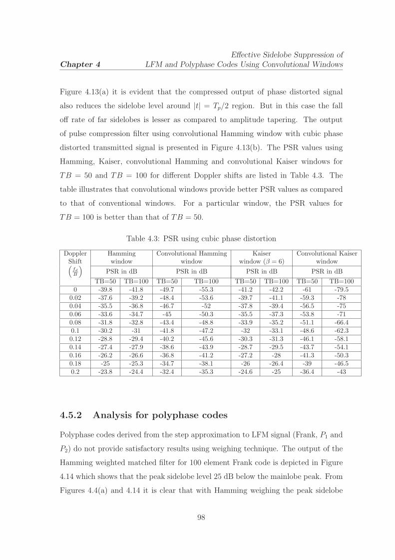
Chapter 4



Figure 4.13(a) it is evident that the compressed output of phase distorted signal

also reduces the sidelobe level around |t| = Tp/2 region. But in this case the fall

off rate of far sidelobes is lesser as compared to amplitude tapering. The output

of pulse compression filter using convolutional Hamming window with cubic phase

distorted transmitted signal is presented in Figure 4.13(b). The PSR values using

Hamming, Kaiser, convolutional Hamming and convolutional Kaiser windows for

TB = 50 and TB = 100 for different Doppler shifts are listed in Table 4.3. The

table illustrates that convolutional windows provide better PSR values as compared

to that of conventional windows. For a particular window, the PSR values for

TB = 100 is better than that of TB = 50.

Table 4.3: PSR using cubic phase distortion

Doppler Hamming Convolutional Hamming Kaiser Convolutional KaiserShift window window window (β = 6) window(

fd

B

)

PSR in dB PSR in dB PSR in dB PSR in dB

TB=50 TB=100 TB=50 TB=100 TB=50 TB=100 TB=50 TB=1000 -39.8 -41.8 -49.7 -55.3 -41.2 -42.2 -61 -79.5

0.02 -37.6 -39.2 -48.4 -53.6 -39.7 -41.1 -59.3 -780.04 -35.5 -36.8 -46.7 -52 -37.8 -39.4 -56.5 -750.06 -33.6 -34.7 -45 -50.3 -35.5 -37.3 -53.8 -710.08 -31.8 -32.8 -43.4 -48.8 -33.9 -35.2 -51.1 -66.40.1 -30.2 -31 -41.8 -47.2 -32 -33.1 -48.6 -62.30.12 -28.8 -29.4 -40.2 -45.6 -30.3 -31.3 -46.1 -58.10.14 -27.4 -27.9 -38.6 -43.9 -28.7 -29.5 -43.7 -54.10.16 -26.2 -26.6 -36.8 -41.2 -27.2 -28 -41.3 -50.30.18 -25 -25.3 -34.7 -38.1 -26 -26.4 -39 -46.50.2 -23.8 -24.4 -32.4 -35.3 -24.6 -25 -36.4 -43

4.5.2 Analysis for polyphase codes

Polyphase codes derived from the step approximation to LFM signal (Frank, P1 and

P2) do not provide satisfactory results using weighing technique. The output of the

Hamming weighted matched filter for 100 element Frank code is depicted in Figure

4.14 which shows that the peak sidelobe level 25 dB below the mainlobe peak. From

Figures 4.4(a) and 4.14 it is clear that with Hamming weighing the peak sidelobe

98

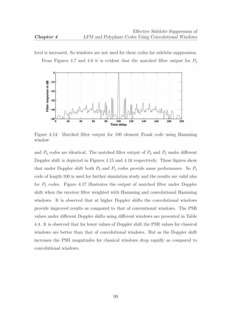
Chapter 4



level is increased. So windows are not used for these codes for sidelobe suppression.

From Figures 4.7 and 4.8 it is evident that the matched filter output for P3

0 20 40 60 80 100 120 140 160 180 200−50

−40

−30

−20

−10

0

Time delay

Filt

er r

espo

nse

in d

B

Figure 4.14: Matched filter output for 100 element Frank code using Hammingwindow

and P4 codes are identical. The matched filter output of P3 and P4 under different

Doppler shift is depicted in Figures 4.15 and 4.16 respectively. These figures show

that under Doppler shift both P3 and P4 codes provide same performance. So P4

code of length 100 is used for further simulation study and the results are valid also

for P3 codes. Figure 4.17 illustrates the output of matched filter under Doppler

shift when the receiver filter weighted with Hamming and convolutional Hamming

windows. It is observed that at higher Doppler shifts the convolutional windows

provide improved results as compared to that of conventional windows. The PSR

values under different Doppler shifts using different windows are presented in Table

4.4. It is observed that for lower values of Doppler shift the PSR values for classical

windows are better than that of convolutional windows. But as the Doppler shift

increases the PSR magnitudes for classical windows drop rapidly as compared to

convolutional windows.

99

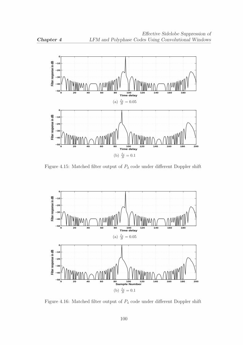
Chapter 4



0 20 40 60 80 100 120 140 160 180−50

−40

−30

−20

−10

0

Time delay

Filte

r res

pons

e in

dB

(a) fd

B= 0.05

0 20 40 60 80 100 120 140 160 180 200−50

−40

−30

−20

−10

0

Time delay

Filte

r res

pons

e in

dB

(b) fd

B= 0.1

Figure 4.15: Matched filter output of P3 code under different Doppler shift

0 20 40 60 80 100 120 140 160 180−50

−40

−30

−20

−10

0

Time delay

Filte

r res

pons

e in

dB

(a) fd

B= 0.05

0 20 40 60 80 100 120 140 160 180 200−50

−40

−30

−20

−10

0

Sample Number

Filte

r res

pons

e in

dB

(b) fd

B= 0.1

Figure 4.16: Matched filter output of P4 code under different Doppler shift

100

Chapter 4



0 20 40 60 80 100 120 140 160 180−50

−40

−30

−20

−10

0

Time delay

Filt

er r

espo

nse

in d

B


(a) fd

B= 0

0 20 40 60 80 100 120 140 160 180−50

−40

−30

−20

−10

0

Time delay

Filt

er r

espo

nse

in d

B


(b) fd

B= 0.05

0 20 40 60 80 100 120 140 160 180−50

−40

−30

−20

−10

0

Time delay

Filt

er r

espo

nse

in d

B


(c) fd

B= 0.1

Figure 4.17: Effect on sidelobes due to Doppler shift

101

Chapter 4



Table 4.4: Comparison of PSR for different Doppler shift

Doppler PSR using Hamming PSR using convolutional

Shift(fd

B) window in dB Hamming window in dB

0.01 -40 -37.170.05 -37.3 -370.1 -32 -36.50.15 -27 -35.70.2 -22.18 -33

Doppler PSR using Hanning PSR using convolutional

Shift(fd

B) window in dB Hanning window in dB

0.01 -40 -36.30.05 -39.6 -36.10.1 -37.1 -35.70.15 -30 -350.2 -25 -33.6

Doppler PSR using Kaiser PSR using convolutional

Shift (fd

B) window in dB (β = 6) Kaiser window in dB

0.01 -40.1 -36.80.05 -37.9 -36.70.1 -33.8 -36.20.15 -28.2 -35.40.2 -23 -34

Doppler PSR using Chebysev PSR using convolutional

Shift(fd

B) window in dB (σ = 50) Chebysev window in dB

0.01 -39 -370.05 -37.9 -36.80.1 -33.3 -36.30.15 -27.8 -35.50.2 -22.7 -33.8

4.6 Conclusion

In this chapter the ability of convolutional windows to suppress the sidelobes are

analyzed and the results are compared with that of conventional windows. Although

the magnitude of PSR at lower Doppler shift in Table 4.1 and 4.4 are better in case of

102

Chapter 4



conventional windows, the convolutional windows provide better PSR value at higher

Doppler shift. In case of LFM signal, to decrease the sidelobes around |t| = Tp

2region

the transmitted signal is modified using amplitude tapering or phase distortion. It is

further demonstrated that the PSR values of amplitude tapered or phase distorted

transmitted signal with convolutional windows are better than that of conventional

windows at all Doppler shift conditions. However, the mainlobe width achieved

using convolutional windows is wider than that of conventional windows.

103

Chapter 5

Efficient Design of SteppedFrequency Pulse Train UsingEvolutionary ComputationTechniques

5.1 Introduction

In high range resolution radar, signals having wide bandwidth are used to get narrow

mainlobe width. Generation of such type of wideband waveforms increases the

overall cost and complexity of the system. The conventional narrowband hardware

used in the radar system may not sustain instantaneous wide bandwidth. To

overcome such limitation the wide bandwidth signal is split into a set of narrowband

signals which are transmitted and received separately. The effect of wideband

signal is obtained by coherently combining the narrowband signals. Such type of

narrowband signals together is called as ‘synthetic wideband waveform’ [109] or

‘stepped frequency waveform’ or ‘frequency jumped train’.

Generally a pulse train consists of N pulses each of duration Tp and pulse

repetition time Tr. Each pulse has a bandwidth B and center frequency step between

the pulses is ∆f . The amplitude and frequency of a stepped frequency LFM pulse

train is shown in Figure 5.1. In the proposed work the values of Tp, B and ∆f

are assumed to remain constant throughout the pulse train and satisfy the condition

104

Chapter 5

Efficient Design of Stepped Frequency Pulse Train Using

Evolutionary Computation Techniques

B > ∆f > 0. One of the advantages of this type of signal is that the interval between

pulses is utilized to adjust the center frequency of other narrowband components of

the radar system. But matched filter output of such signals suffer from grating lobes

for cases when Tp∆f > 1 due to constant frequency step ∆f . These grating lobes

reduce the range resolution capability of the signal and hence these are undesirable.

Figure 5.1: Stepped frequency LFM pulse train

Different techniques for acceptable suppression or complete rejection of grating

lobes are dealt in [110–115]. In [110, 111] grating lobes are reduced by varying

the pulse width of the pulse train which destroys the periodicity of the waveform.

An approach to generate a nonlinear synthetic wideband waveform by distributing

the energy nonuniformly over the desired bandwidth is described in [112]. It

offers improved performance in terms of lower range sidelobes, higher range

resolution and/or reduced grating lobes. Levanon and Mozeson [113] have proposed

an analytical technique to establish the relation between parameters of stepped

frequency LFM pulse train such that the first two grating lobes are nullified. They

have also shown in some cases that nullifying the first two grating lobes leads to

removal of all other grating lobes. To establish the required relation between the

parameters Tp, B and ∆f using this approach for more than two grating lobes is too

difficult. In this chapter PSO based technique is suggested which aims to eliminate

105

Chapter 5



all the grating lobes by judiciously choosing appropriate values of Tp, B and ∆f .

The method presented in [113] does not suppress the range sidelobes that occur

at the output of the matched filter of the receiver. In [114, 115] the LFM pulses

are replaced by nonlinear LFM pulses that suppress the range sidelobes near the

mainlobe along with grating lobes. However, the nonlinear LFM signals are not

Doppler tolerant.

The LFM pulse can be easily generated and more Doppler tolerant than NLFM

pulse. Therefore LFM waveforms are widely used in pulse radar systems. But

the techniques used in [113–115] to suppress the grating lobes of LFM pulse train

ignore the mainlobe width and PSL. The waveform having wide mainlobe width in

its ACF has low range resolution capability and the waveform that yields high peak

sidelobe in its ACF may hide the small targets or cause false target detection. Hence

there is a need to develop an efficient method to determine the parameters of the

stepped frequency LFM pulse train by considering grating lobes, mainlobe width

and PSL. Keeping this fact in view, in this chapter a new optimization is proposed

approach using NSGA-II algorithm to achieve reduced grating lobes, lower sidelobes

and narrow mainlobe width.

5.2 LFM pulse train

The envelope of a constant frequency or unmodulated pulse of duration Tp is given

by

u(t) =1√

Tp

rect

(

t

Tp

)

(5.1)

Frequency modulation is applied to the above constant frequency pulse to get an

LFM signal and its complex envelope is represented as

u1(t) =1√

Tp

rect

(

t

Tp

)

exp(jπkt2) (5.2)

where k is the frequency slope of the LFM signal and is defined as

k = ±B1

Tp

(5.3)

106

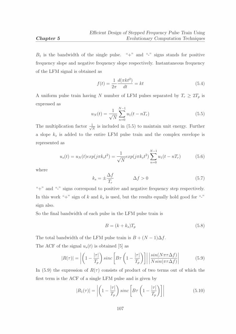
Chapter 5



B1 is the bandwidth of the single pulse. “+” and “-” signs stands for positive

frequency slope and negative frequency slope respectively. Instantaneous frequency

of the LFM signal is obtained as

f(t) =1

2π

d(πkt2)

dt= kt (5.4)

A uniform pulse train having N number of LFM pulses separated by Tr ≥ 2Tp is

expressed as

uN(t) =1√N

N−1∑

n=0

u1(t − nTr) (5.5)

The multiplication factor 1√N

is included in (5.5) to maintain unit energy. Further

a slope ks is added to the entire LFM pulse train and the complex envelope is

represented as

us(t) = uN(t)exp(jπkst2) =

1√N

exp(jπkst2)

N−1∑

n=0

u1(t − nTr) (5.6)

where

ks = ±∆f

Tr

∆f > 0 (5.7)

“+” and “-” signs correspond to positive and negative frequency step respectively.

In this work “+” sign of k and ks is used, but the results equally hold good for “-”

sign also.

So the final bandwidth of each pulse in the LFM pulse train is

B = (k + ks)Tp (5.8)

The total bandwidth of the LFM pulse train is B + (N − 1)∆f .

The ACF of the signal us(t) is obtained [5] as

|R(τ)| =

∣

∣

∣

∣

(

1 − |τ |Tp

)

sinc

[

Bτ

(

1 − |τ |Tp

)]∣

∣

∣

∣

∣

∣

∣

∣

sin(Nπτ∆f)

Nsin(πτ∆f)

∣

∣

∣

∣

(5.9)

In (5.9) the expression of R(τ) consists of product of two terms out of which the

first term is the ACF of a single LFM pulse and is given by

|R1(τ)| =

∣

∣

∣

∣

(

1 − |τ |Tp

)

sinc

[

Bτ

(

1 − |τ |Tp

)]∣

∣

∣

∣

(5.10)

107

Chapter 5



and the second term

|R2(τ)| =

∣

∣

∣

∣

sin(Nπτ∆f)

Nsin(πτ∆f)

∣

∣

∣

∣

(5.11)

produces the grating lobes at τg = g∆f

where g = 1, 2, 3.... ⌊Tp∆f⌋. These grating

lobes appear in the form of high spikes and reduce the range resolution potential of

the waveform. Nullifying or suppressing these grating lobes essentially depends upon

the occurrence of nulls or minima of |R1(τ)| at τg. In [113] an analysis is provided

that sets up simple relations between the pulse time duration Tp, its bandwidth

B and frequency step ∆f to nullify first two grating lobes of an LFM pulse train.

However, in some cases nullifying two grating lobes also removes all grating lobes.

Equation (5.9) can be written as

∣

∣

∣

∣

R

(

τ

Tp

)∣

∣

∣

∣

=

∣

∣

∣

∣

(

1 −∣

∣

∣

∣

τ

Tp

∣

∣

∣

∣

)

sinc

[

TpBτ

Tp

(

1 −∣

∣

∣

∣

τ

Tp

∣

∣

∣

∣

)]∣

∣

∣

∣

∣

∣

∣

∣

∣

sin(Nπ∆fTpτTp

)

Nsin(πTp∆f τTp

)

∣

∣

∣

∣

∣

,

∣

∣

∣

∣

τ

Tp

∣

∣

∣

∣

≤ 1

(5.12)

From (5.9), (5.10), (5.11) and (5.12) it is clear that |R(τ)|, |R1(τ)| and |R2(τ)| are

functions of Tp∆f and TpB only for a given value of N . Figure 5.2 shows the plots

of |R1(τ)|, |R2(τ)| and ACF for Tp∆f = 3, TpB = 4.5 and N = 8. It is observed

that all the grating lobes are completely removed. For comparison purpose the ACF

obtained with fixed frequency pulse train is shown in Figure 5.3 in which the grating

lobes are prominent. The nullification of first two grating lobes always does not

guarantee that all other grating lobes will be nullified or suppressed because the

nulls of |R1(τ)| do not occur periodically while the peaks of |R2(τ)| occur with a

period 1∆f

. The mainlobe width depends on the first overall null of the expressions

|R1(τ)| and |R2(τ)|. The first null of |R2(τ)| occurs at 1NTp∆f

and the first null of

|R1(τ)| occurs at 1TpB

approximately if TpB >> 1. So the location of first null of

ACF is given byτ1stnull

Tp

= min

(

1

TpB,

1

NTp∆f

)

(5.13)

N∆f should be always greater than B in order to get a meaningful increase in

bandwidth. So delay resolution is principally determined by |R2(τ)| which is equal

to 1NTp∆f

.

108

Chapter 5



0 0.1 0.2 0.3 0.4 0.5 0.6 0.7 0.8 0.9 10

0.2

0.4

0.6

0.8

1

| R1(τ

) |, |

R2(τ

) |

0 0.1 0.2 0.3 0.4 0.5 0.6 0.7 0.8 0.9 1−60

−50

−40

−30

−20

−10

0

τ/ Tp

AC

F in

dB

Figure 5.2: Stepped frequency LFM pulse for Tp∆f = 3, TpB = 4.5 and N = 8.Top: |R1(τ)| (dash) and |R2(τ)| (solid). Bottom: ACF (in dB)

0 0.1 0.2 0.3 0.4 0.5 0.6 0.7 0.8 0.9 10

0.2

0.4

0.6

0.8

1

| R1(τ

) |,|

R2(τ

) |

0 0.1 0.2 0.3 0.4 0.5 0.6 0.7 0.8 0.9 1−60

−40

−20

0

τ / Tp

AC

F in

dB

Figure 5.3: Stepped frequency LFM pulse for Tp∆f = 3, TpB = 0 and N = 8. Top:|R1(τ)| (dash) and |R2(τ)| (solid). Bottom: ACF (in dB)

109

Chapter 5




The grating lobes reduce range resolution ability of the pulse train. So it is required

to suppress or nullify these grating lobes. In Section 5.3.1 a problem is formulated

in which the PSO is used to determine the parameters of stepped frequency pulse

train to nullify the grating lobes.

The problem of suppression of grating lobes, minimization of mainlobe width

and peak sidelobe level has been formulated in two different ways in a multiobjective

framework which are presented in Sections 5.3.2 and 5.3.3.

5.3.1 Problem formulation -1

The function defined in (5.10) must be minimum or zero at τ = τg, so that the

grating lobes would be suppressed or nullified. The fitness function which is to be

minimized using PSO is defined as

f1 =∑

g

∣

∣

∣

∣

(

1 − |τg|Tp

)

sinc

[

Bτ

(

1 − |τg|Tp

)]∣

∣

∣

∣

(5.14)

subject to N∆f > B.

By choosing suitable values for TpB and Tp∆f the grating lobes as well as sidelobes

in ACF can be suppressed. The value of TpB is chosen such that TpB = (c+1)Tp∆f

(where c is a positive number) to ensure B > ∆f , so that there will be some

frequency overlap between the pulses in spite of the frequency steps. If f1 = 0 then

each term in the summation is zero which results in complete elimination of grating

lobes otherwise the grating lobes are suppressed to a minimum level. PSO is used

to find out the required values of Tp∆f and c so that f1 is minimized.


The peak sidelobe should be as low as possible compared to the mainlobe so that

the target will be easily identified. NSGA-II algorithm is used to choose the

values of Tp∆f and c to achieve reduced grating lobes and minimum peak sidelobe

110

Chapter 5



level simultaneously. The two objective functions which are to be simultaneously

optimized are expressed as follows:

Minimize f2 = max|R1(τg)| where g = 1, 2, 3..... ⌊Tp∆f⌋Minimize f3 = PSR in dB

subject to N∆f > B


The range resolution of stepped frequency LFM pulse train depends upon the

mainlobe width of ACF and is given by 1NTp∆f

for NTp∆f > TpB. In the literature

generally weighing technique is used to suppress the sidelobes of an LFM pulse. The

weighing technique adds more emphasis on the center frequencies as compared to the

end frequencies. As a result the sidelobes are suppressed and mainlobe is widened,

which reduces the range resolution capability of the LFM signal. This effect is also

applicable for stepped frequency LFM pulse train as the condition B > ∆f > 0 is

assumed. The values of Tp∆f and c are chosen by using a multiobjective algorithm

in such a way that the mainlobe width is lowered (for high range resolution) and

the sidelobes are suppressed. The effect of grating lobes is reduced by putting a

constraint so that the grating lobes are below a threshold level i.e. |R1(τg)| < ǫ.

The fitness functions which are to be optimized simultaneously are defined as

Minimize f3 = PSR in dB

Minimize f4 = 1NTp∆f

subject to NTp∆f > TpB and |R1(τg)| < ǫ.

5.4 Techniques used

In this chapter single objective evolutionary algorithm, PSO, and multiobjective

algorithm, NSGA-II, are used to determine the parameters of the LFM pulse train.

An overview of each of the algorithms is presented in sequel.

111

Chapter 5



5.4.1 Particle swarm optimization

The PSO was introduced by Kennedy and Eberhart [116] in 1995 which is a

population based and self adaptive search optimization technique. This algorithm

was developed based on simulation of animals social behavior such as bird flocking,

fish schooling etc. Like other population based evolutionary computation algorithm

such as GA, the PSO starts with random initialization of population, called as

swarm, in the search space and each individual is called as a particle. Unlike GA,

the PSO have not direct combination of genetic materials between the particles

during the search. The PSO algorithm employs the social behavior of the particle

in the swarm. Hence, it finds the global solution by adjusting the trajectory of each

particle towards its own best solution and towards the best particle of the swarm

in each generation [116–118]. The PSO is very popular because of the simplicity

of implementation of the algorithm and ability to converge quickly to a acceptable

good solution.

In PSO, the trajectory of each particle in search space is altered according to its

own velocity, own flying experience and flying experience of other particles in the

swarm.

The position of ith particle in D dimensional search space is given by

xi = [xi1, xi2, ..... xiD]T (5.15)

and the velocity of ith particle is expressed as

vi = [vi1, vi2, ..... viD]T (5.16)

The fitness function value is found out according to the user defined fitness function

which is to be optimized.

Let pbesti be the best position i.e. the best fitness value obtained by the ith

particle at time t. So

pbesti = [pbesti1, pbesti2, ..... pbestiD]T (5.17)

112

Chapter 5



The fittest particle found in the swarm at time t is

gbest = [gbest1, gbest2, ...... gbestD]T (5.18)

The position and velocity of each particle is updated as

vid(t + 1) = wvid(t) + c1r1(pbestid(t) − xid(t)) + c2r2(gbestd(t) − xid(t)) (5.19)

xid(t + 1) = xid(t) + vid(t + 1) (5.20)

where d = 1, 2, ....D and w is a positive constant or positive linear or nonlinear

function of time [119, 120]. w is called inertia weight which plays the role of

balancing the local and global searches. c1 and c2 are two positive constants known

as acceleration coefficients and r1 and r2 are two random numbers in between 0

and 1. The first term in the right hand side of (5.19) corresponds to the previous

velocity which provides the necessary momentum and the second term stands for the

cognitive component which represents the personal thinking of each particle. The

cognitive component promotes the particles to move towards their own best position.

The third term is called as social component which constitutes the cooperative effect

of the particles in finding the global optimal solution. The social component always

drags the particle towards the global particle found so far.

The population is initialized with random positions and random velocities are

assigned to each particle. The fitness function value is evaluated according to defined

objective function i.e. to be optimized. At each generation the velocity and position

of the each particle are updated according to (5.19) and (5.20) respectively. In a

particular generation if a particle finds better position than previously found then

its location is stored in the memory. A maximum velocity i.e. Vmaxdis defined for

each dimension for the velocity vector vid in order to control the excessive roaming

of the particle outside the defined search space. If vid exceeds Vmaxd, then vid is set

to Vmaxd.

113

Chapter 5



5.4.2 NSGA-II

The NSGA-II which is described in Chapter 2 dealt with binary coded chromosome.

In this chapter the real coded chromosomes are used and the genetic operators

such as crossover and mutation are different than binary coded GA. For real coded

chromosomes simulated binary crossover and polynomial mutation are used to

generate offsprings. The steps such as population initialization, fitness function

evaluation, crowding distance assignment, selection, recombination process are same

as explained in Section 2.3.2 except the genetic operators.

Genetic operators:

Genetic operators such as crossover and mutation are used to explore and exploit

new and better solution from the existing solutions in the objective space. Real

coded NSGA-II uses simulated binary crossover [121,122] and polynomial mutation

[122,123] to produce offspring.

1. Simulated binary crossover: A random number y is generated between 0 and

1. From a defined probability distribution function (pdf) another variable α

is found such that the area under the pdf from 0 to α is equal to y. The pdf

is defined as

P (α) =

0.5 (ηc + 1) αηc if α ≤ 1

0.5 (ηc + 1) 1αηc+2 if α > 1

(5.21)

where ηc is the distribution index for crossover. This pdf is obtained by using

the transformation

α (y) =

(2y)1

(ηc+1) if y ≤ 0.5

1

[2(1−y)]1

(ηc+1)otherwise

(5.22)

After obtaining α the off-spring children are computed as

c1,k =1

2[(1 − αk) x1,k + (1 + αk) x2,k] (5.23)

c2,k =1

2[(1 + αk) x1,k + (1 − αk) x2,k] (5.24)

114

Chapter 5



where αk is the value of α for kth component of the chromosome.

ci,k is the kth component of ith child.

xi,k is the kth component of ith parent which is selected for crossover.

2. Polynomial mutation: Mutation in GA restores lost or unexpected genetic

materials into the solution to avoid convergence of the algorithm into a

sub-optimal solution. The polynomial mutation is defined as

ck = xk +(

xuk − xl

k

)

δk (5.25)

where ck is the mutated child produced from parent xk. xuk and xl

k are the

upper and lower bound of xk. δk is the small variation which is obtained by

δk =

(2rk)1

ηm+1 − 1 if rk ≤ 0.5

1 − [2 (1 − rk)]1

ηm+1 otherwise(5.26)

where ηm is the distribution index for mutation and rk is a random number in

between 0 and 1.

5.5 Determination of parameters of LFM pulse

train

5.5.1 Using PSO

The fitness function defined in (5.14) is minimized to determine the parameters of

LFM pulse train. The various steps are

1. The population of size M is initialized randomly in the given search space and

each particle in the population consists of two dimensions corresponds to Tp∆f

and c. Random velocities are assigned to each particle .

2. The fitness function for each chromosome is evaluated according to (5.14).

The particle having best fitness value called as gbest. Initially the pbest for

a particle assumed as particle position itself.

115

Chapter 5



3. The velocity and position of each particle are updated as given in (5.19) and

(5.20) respectively.

4. The fitness function value is evaluated for the new position for each particle

and compared with the corresponding pbest positions fitness value. If for a

particle the new position fitness is better than that of pbest then the pbest

will be replaced by new particle. The particle having best fitness value among

all the pbests is selected as gbest.

Steps 3 and 4 repeated until the predefined condition is satisfied.

5.5.2 Using NSGA-II

The problems defined in Sections 5.3.2 and 5.3.3 use this algorithm to find the desired

parameter values of LFM pulse train. The various steps involved are

1. A population having M chromosomes is randomly initialized and each

chromosome contains two random values corresponds to Tp∆f and c.

2. The fitness function values f2 and f3 (f3 and f4 for problem-3) are evaluated

as given in Section 5.3.2. (Section 5.3.3 for problem-3)

3. The chromosomes are sorted using nondominated sort and all possible fronts

are obtained as in Section 2.3.2.

4. The crowding distance for chromosomes in each front are evaluated according

to the procedure explained in Section 2.3.2.

5. The chromosomes are selected using binary tournament selection according to

Section 2.3.2.

6. The selected chromosomes undergo for genetic operations such as crossover

and mutation to produce offspring as explained Section 5.4.2.

7. The off-spring population is combined with parent population and the best M

chromosome selected for next generation as described in Section 2.3.2

116

Chapter 5



Steps from 5 to 7 are repeated until the maximum number of generations.


Simulation studies are carried out according to the problem formulation as presented

in Section 5.3. The techniques explained in Section 5.4 are used for grating lobe

suppression. To carry out PSO based estimation task the swarm size and number of

generations are chosen to be 100 and 50 respectively. This choice is based on trial

and error so as to achieve the best possible performance. The particles are randomly

initialized in the defined search space Tp∆f ∈ [2, 15] and c ∈ [1, 10] . The values

of c1 and c2 are taken as 2. The velocity and position of the particles are updated

according to (5.19) and (5.20) respectively. At the end of all the generations if f1

attains a zero value then each term of the right hand side of (5.14) becomes zero

which means complete elimination of grating lobes. There are more than one set

of Tp∆f and c present in the defined search space for which f1 = 0. At the end of

all the generations the best particle is saved and the program executed repeatedly

to get the other distinct best solutions. The values of Tp∆f , TpB and B/∆f for

N = 8 are listed in Table 5.1 for f1 = 0. Figures 5.4 and 5.5 show the plots of

|R1(τ)|, |R2(τ)| and |R(τ)| for Tp∆f = 2.5, TpB = 12.5 and Tp∆f = 4, TpB = 16

respectively. From these figures it is observed that the peaks of the |R2(τ)| (grating

lobes) exactly coincide with the nulls of |R1(τ)|, as a result there are nulls in |R(τ)|at those points.

NSGA-II algorithm is employed for optimization of f2 and f3 associated in

problem 2. The population size and the number of generations are taken to be

100 and 50 respectively. The distribution indices for crossover (ηc) and mutation

(ηm) are chosen as 20 each. The probabilities of crossover and mutation are set to

be 0.9 and 0.1 respectively. Tp∆f and c are the two variables judiciously chosen

by the NSGA-II algorithm to get low sidelobe level and reduced grating lobes. The

initialized population is sorted based on nondomination and each solution is assigned

with a crowding distance. The selection, crossover, mutation and recombination are

117

Chapter 5



0 0.1 0.2 0.3 0.4 0.5 0.6 0.7 0.8 0.9 10

0.2

0.4

0.6

0.8

1

|R1(τ

)|,

|R2(τ

)|

0 0.1 0.2 0.3 0.4 0.5 0.6 0.7 0.8 0.9 1−60

−40

−20

0

τ/Tp

AC

F [

dB

]

Figure 5.4: Stepped frequency LFM pulse for Tp∆f = 2.5, TpB = 12.5 and N = 8.Top: |R1(τ)| (dash) and |R2(τ)| (solid). Bottom: ACF (in dB)

0 0.1 0.2 0.3 0.4 0.5 0.6 0.7 0.8 0.9 10

0.2

0.4

0.6

0.8

1

|R1(τ

)|,

|R

2(τ

)|

0 0.1 0.2 0.3 0.4 0.5 0.6 0.7 0.8 0.9 1−60

−40

−20

0

τ/Tp

AC

F [

dB

]

Figure 5.5: Stepped frequency LFM pulse for Tp∆f = 4, TpB = 16 and N = 8. Top:|R1(τ)| (dash) and |R2(τ)| (solid). Bottom: ACF (in dB)

118

Chapter 5



Table 5.1: Values of Tp∆f , TpB obtained for N = 8 and f1 = 0

Tp∆f TpB = (c + 1)Tp∆f B∆f

= c + 1

2 4 22.5 12.5 53 9 3

3.5 24.5 74 16 45 12.5 2.56 36 67 24.5 3.59 40.5 4.511 60.5 5.513 84.5 6.515 112.5 7.5

carried out for each generation according the procedure given in Section 5.4. Figure

5.6 illustrates Pareto front obtained for Tp∆f ∈ [2, 10], c ∈ [2, 10] and N = 8. This

Pareto front provides the trade-off solutions between grating lobe and the PSR. It

is evident from Figure 5.6 that for all the solutions the sidelobes are below 30 dB

as compared to their respective mainlobes. All the solutions in the Pareto front are

nondominant and a particular solution from the front is chosen according to the

requirements of the application such as low sidelobe level or low grating lobes. For

different values of Tp∆f and TpB corresponding values of |R1(τ)|, |R2(τ)| and ACF

are shown in Figures. 5.7 to 5.9. In Figure 5.7 the nulls of |R1(τ)| exactly falls

on the grating lobes of |R2(τ)| which means that all the grating lobes are canceled

i.e. f2 = 0. In Figure 5.9, the maximum grating lobe amplitude is 0.021 which

is prominently observed around τ/Tp = 0.7 in ACF. But the sidelobes occurring

in Figure 5.7 are below 30.7753 dB from its mainlobe and that of in Figure 5.9 is

32.5 dB below its mainlobe. Therefore the parameter values of stepped frequency

LFM pulse train are chosen according to the requirement of application. If it is

required to suppress all the grating lobes below a certain value ǫ, then a constraint

i.e. f1 < ǫ is associated with the optimization process. Different Pareto fronts can

119

Chapter 5



0 0.005 0.01 0.015 0.02 0.025−33

−32.5

−32

−31.5

−31

−30.5

maximum grating lobe amplitude (f2)

PSR

in d

B (f 3)

Figure 5.6: Pareto front obtained using NSGA-II for Tp∆f ∈ [2, 10], c ∈ [2, 10] andN = 8

be obtained by varying the upper and lower limits of Tp∆f and c depending upon

their ranges for that particular application. For Tp∆f ∈ [2, 10], c ∈ [2, 10], ǫ = 0.01,

N = 8 and Tp∆f ∈ [5, 30], c ∈ [2, 10], ǫ = 0.01, N = 8 the Pareto fronts are

depicted in Figures 5.10 and 5.11 respectively. The NSGA-II algorithm facilitates

for choosing the parameters from a set of available optimal parameters according

to the requirements of the system under consideration. Small grating lobes or low

sidelobes can be achieved by choosing an appropriate solution from Pareto front.

Suitable overlap ratio, i.e. B∆f

= c + 1, is accomplished by properly defining lower

and higher limit of c during population initialization.

For the third problem the population size and number of generations are chosen

to be 200 and 50 for optimizing the values of f3 and f4. Same set of previously

chosen parameters of NSGA-II algorithm is used in this case. The population is

randomly initialized for two parameters Tp∆f and c for the given lower and upper

limit. The initialized population is sorted according to the nondomination sorting

and the process of selection, crossover, mutation and recombination are carried out

for each generation according to the procedure laid down in Section 5.5.2. For

Tp∆f ∈ [2, 10], c ∈ [2, 5], ǫ = 0.01 and N = 8 the Pareto front is shown in the Figure

5.12. This Pareto front provides a trade-off between the grating lobe and mainlobe

width. A solution from the Pareto front is chosen according to the requirements of

120

Chapter 5



0 0.1 0.2 0.3 0.4 0.5 0.6 0.7 0.8 0.9 10

0.2

0.4

0.6

0.8

1

|R1(τ

)|,|R

2(τ

)|

0 0.1 0.2 0.3 0.4 0.5 0.6 0.7 0.8 0.9 1−60

−40

−20

0

τ / Tp

AC

F in

dB

Figure 5.7: Stepped frequency LFM pulse for Tp∆f = 2, c = 5, TpB = 12 andN = 8. Top: |R1(τ)| (dash) and |R2(τ)| (solid). Bottom: ACF (in dB)

0 0.1 0.2 0.3 0.4 0.5 0.6 0.7 0.8 0.9 10

0.2

0.4

0.6

0.8

1

| R

1(τ

), R

2(τ

) |

0 0.1 0.2 0.3 0.4 0.5 0.6 0.7 0.8 0.9 1−60

−40

−20

0

τ / Tp

AC

F in

dB

Figure 5.8: Stepped frequency LFM pulse for Tp∆f = 2, c = 5.1412, TpB = 12.2824and N = 8. Top: |R1(τ)| (dash) and |R2(τ)| (solid). Bottom: ACF (in dB)

121

Chapter 5



0 0.1 0.2 0.3 0.4 0.5 0.6 0.7 0.8 0.9 10

0.2

0.4

0.6

0.8

1

| R

1(τ

) |, |R

2(τ

) |

0 0.1 0.2 0.3 0.4 0.5 0.6 0.7 0.8 0.9 1−60

−40

−20

0

τ/Tp

AC

F in

dB

Figure 5.9: Stepped frequency LFM pulse for Tp∆f = 2.8721, c = 5.0978, TpB =17.5135 and N = 8. Top: |R1(τ)| (dash) and |R2(τ)| (solid). Bottom: ACF (in dB)

0 0.001 0.002 0.003 0.004 0.005 0.006 0.007 0.008 0.009 0.01−31.8

−31.6

−31.4

−31.2

−31

−30.8

−30.6

Maximum grating lobe amplitude (f2)

PSR

in dB

(f3)

Figure 5.10: Pareto front obtained using NSGA-II for Tp∆f ∈ [2, 10] c ∈ [2, 10],ǫ = 0.01 and N = 8

122

Chapter 5



0 0.001 0.002 0.003 0.004 0.005 0.006 0.007 0.008 0.009 0.01−28.85

−28.8

−28.75

−28.7

−28.65

−28.6

−28.55

−28.5

−28.45

−28.4

Maximum gratiing lobe amplitude (f2)

PSR

in dB

(f 3)

Figure 5.11: Pareto front obtained using NSGA-II for Tp∆f ∈ [5, 30], c ∈ [2, 10],ǫ = 0.01 and N = 8

0.01 0.015 0.02 0.025 0.03 0.035 0.04 0.045−32

−31

−30

−29

−28

−27

−26

−25

−24

−23

−22

f4

f 3

Figure 5.12: Pareto front obtained using NSGA-II for Tp∆f ∈ [2, 10], c ∈ [2, 5],ǫ = 0.01 and N = 8

application under consideration. If the application demands high range resolution,

a solution having low value of f4 is chosen and if it requires low sidelobe level, a

solution corresponds to high magnitude of f3 is chosen. Figures 5.13 to 5.16 show

|R1(τ)|, |R2(τ)| and ACF for different values of Tp∆f , c and ǫ = 0.01. It is evident

from the figures that reduction of peak sidelobe is achieved at the cost of increase

in mainlobe width or reduction in range resolution.

123

Chapter 5



0 0.1 0.2 0.3 0.4 0.5 0.6 0.7 0.8 0.9 10

0.2

0.4

0.6

0.8

1

| R

1(τ

) |,| R

2(τ

) |

0 0.1 0.2 0.3 0.4 0.5 0.6 0.7 0.8 0.9 1−60

−40

−20

0

τ / Tp

AC

F in

dB


0 0.1 0.2 0.3 0.4 0.5 0.6 0.7 0.8 0.9 10

0.2

0.4

0.6

0.8

1

|R1(τ

)|,

|R2(τ

)|

0 0.1 0.2 0.3 0.4 0.5 0.6 0.7 0.8 0.9 1−60

−40

−20

0

τ / Tp

AC

F in

dB


124

Chapter 5



0 0.1 0.2 0.3 0.4 0.5 0.6 0.7 0.8 0.9 10

0.2

0.4

0.6

0.8

1

| R

1(τ

) |, | R

2(τ

) |

0 0.1 0.2 0.3 0.4 0.5 0.6 0.7 0.8 0.9 1−60

−40

−20

0

τ / Tp

AC

F in

dB


0 0.1 0.2 0.3 0.4 0.5 0.6 0.7 0.8 0.9 10

0.2

0.4

0.6

0.8

1

| R1(τ

) |,

| R2(τ

) |

0 0.1 0.2 0.3 0.4 0.5 0.6 0.7 0.8 0.9 1−60

−40

−20

0

τ / Tp

AC

F in

dB

Figure 5.16: Stepped frequency LFM pulse for Tp∆f = 3, c = 5, TpB = 18 andN = 8. Top: |R1(τ)| (dash) and |R2(τ)| (solid). Bottom: ACF (in dB)

125

Chapter 5



5.7 Conclusion

Frequency stepping technique is mostly used in radar technology to achieve high

range resolution by combining the effect of narrowband pulses that span in the

desired bandwidth. The drawback of such type of waveform is the presence of the

grating lobes. In this chapter the PSO algorithm is used to determine the parameters

of LFM pulse train for which all the grating lobes are nullified. Using the PSO various

combinations of Tp∆f and TpB are found for which all the grating lobes are nullified

and listed in Table 5.1. Changing the limits of Tp∆f and c more combination of

Tp∆f and TpB can be found for which all the grating lobes are nullified.

The multiobjective NSGA-II algorithm has been applied to determine the

parameters of stepped frequency pulse train to get reduced grating lobes, low

sidelobes and narrow mainlobe width at the matched filter output of the pulse train.

The multiobjective optimization algorithm enables to provide trade off solutions

between different objectives through Pareto front that contains nondomination

solutions. In the proposed work the multiobjective problem has been formulated

in two different manners. One formulation provides the trade-off solutions between

grating lobes and peak sidelobe and the other provides the trade-off solutions

between peak sidelobe and mainlobe width.

126

Chapter 6

Conclusion and Future Work

6.1 Conclusion

In this chapter, the conclusion of the whole thesis is presented and future research

problems are outlined for further investigation in the same or related topics. In

this thesis investigation has been made on developing efficient pulse compression

techniques for phase and frequency modulated waveforms. The main contribution

of the thesis is the use of neural network structures and evolutionary computation

techniques for pulse compression.

Biphase codes of longer sequences having low PSL and high MF are important

research area in the field of radar signal processing. There is no available technique

to generate a certain length code for a given PSL and/or MF. In this thesis a

multiobjective algorithm (NSGA-II) is presented to generate the biphase codes of

length 49 to 59 using PSL and MF as two different objective functions. The use

of NSGA-II algorithm has provided more than one nondominated solutions and a

particular code is to be selected depending upon specific situation. This algorithm

in general can be applied to generate codes of any length.

Mismatch filters are used to provide better PSR than that of matched filter of

a given sequence. Several ANN based mismatch filters are used to achieve reduced

sidelobes for 13-bit and 35-bit Barker codes at the output of the filter. In this work,

the RNN and RRBF structures are proposed to use as a pulse compression filter

127

Chapter 6 Conclusion and Future Work

which have been provided better performance in terms of PSR under various adverse

conditions such as noise, multiple target and Doppler shift. The performance of the

proposed methods is compared to that of MLP and RBF based pulse compression

techniques. The comparison study reveals that the RRBF based pulse compression

technique performs the best among others.

Biphase codes can be easily generated and their matched filters implementation

are also simple. These advantages are achieved at the cost of higher sidelobes.

Polyphase codes have lower sidelobes compared to biphase codes for a certain length

code. The LFM signals are more Doppler tolerant than phase coded signals. Hence,

phase codes such as Frank, P1, P2, P3 and P4 codes are derived from the LFM signals

to get the advantages of the Doppler shift performance of LFM signal. The PSRs

offered by LFM and polyphase codes are not adequate for many radar applications.

Various windows are used to suppress the sidelobe of LFM and polyphase codes. In

this thesis the use of convolutional windows are proposed as the weighing function

at the receiver to get better PSR values at higher Doppler shifts compared to that

of conventional windows. Amplitude tapering and phase distortion techniques are

employed to modify the transmitted LFM signal and the convolutional window

is used as the weighing function at the receiver offers better PSR values that of

conventional windows.

In high range resolution radar the bandwidth of the signal should be large

to achieve narrow mainlobe width. To overcome the difficulty of generation and

processing, the wideband signal is split into a number of narrowband signals which

together called as stepped frequency waveform. The ACF of stepped frequency

LFM pulse train suffers from grating lobes for Tp∆f > 1. Hence the range resolution

capability of the waveform is reduced. A PSO algorithm based technique is proposed

to choose the parameters of LFM pulse train to nullify or suppress the grating

lobes. Further, a widely used multiobjective NSGA-II algorithm based approach

is proposed to determine the optimum parameters of LFM pulse train to achieve

reduced grating lobes, low sidelobes and narrow mainlobe width. The multiobjective

128

Chapter 6 Conclusion and Future Work

problem has been formulated in two different ways. One formulation provides the

trade-off solutions between grating lobes and peak sidelobe and the other provides

the trade-off between peak sidelobe and mainlobe width.

6.2 Future work

The research work presented in the thesis can be further extended in following ways.

• Genetic operators such as crossover and mutation are important operations in

GA and NSGA-II. Better biphase codes can be designed by employing different

variant of these operators.

• Better mismatch filters can be developed using polynomial neural network and

support vector machine for sidelobe suppression and the performance can be

compared with existing methods.

• Time-frequency analysis such as short time Fourier transform, wavelet

transform and S-transform can be used for LFM signals to extract Doppler

information.

• The LFM signal can be replaced by Doppler tolerant hyperbolic frequency

modulated pulse in the pulse train and the multiobjective algorithms can be

employed to enhance sidelobe suppression.

129

Bibliography

[1] M. I. Skolnik, Introduction to radar system. New York: McGraw-Hill, 1980.

[2] C. E. Cook and M. Bernfeld, Radar signals: An introduction to theory and

application. Academic Press, New York, 1967.

[3] D.K. Barton, Pulse Compression. Artech House, 1975.

[4] A.W. Rihaczek, Principle of high resolution radar. McGraw Hill, New York,

1969.

[5] N. Levanon and E. Mozeson, Radar Signals. Wiley New York, 2004.

[6] P. M. Woodward, Probability and information theory, with application to radar.

Pergamon Press, Oxford, 1953.

[7] A.M. Boehmer, “Binary pulse compression codes,” IEEE Trans. on Inf. Theory,

vol. 13, no. 2, pp. 156-167, Apr 1967.

[8] R.H. Barker, “Group Synchronization of Binary Digital Systems,” Commun.

Theory, pp. 273-287, 1953.

[9] M. I. Skolnik, Radar Handbook. New York: McGraw-Hill (2nd ed.), 1990.

[10] J. Lindner, “Binary sequences up to length 40 with best possible autocorrelation

function,” Electron. Lett., vol. 11, no. 21, p. 507, Oct. 1975.

[11] M. N. Cohen, M. R. Fox, and J. M. Baden, “Minimum peak sidelobe pulse

compression codes,” in Proc. IEEE Int. Radar Conf., pp. 633-639, 1990.

[12] F. Hu, P. Z. Fan, M. Darnell and F. Jin, “Binary sequences with good aperiodic

autocorrelation functions obtained by neural network search,” Electron. Lett., vol.

33, no. 8, pp. 688-690, Apr. 1997.

130

Bibliography

[13] S. Wang, “Efficient heuristic method of search for binary sequences with good

aperiodic autocorrelations,” Electron. Lett., vol. 44, no. 12, pp. 731-732, June

2008.

[14] B. Militzer, M. Zamparelli and D. Beule, “Evolutionary search for low

autocorrelated binary sequences,” IEEE Trans. on Evol. Comput., vol. 2, no.

1, pp. 34-39, Apr. 1998.

[15] X. Deng and P. Fan, “New binary sequences with good aperiodic

autocorrelations obtained by evolutionary algorithm,” IEEE Comm. Lett., vol.

3, no. 10, pp. 288-290, Oct. 1999.

[16] K. R. Rajeswari and N. Gangatharan, “Algorithm for design of pulse

compression radar codes,” Electron. lett., vol. 39, no. 11, pp. 865-867, May 2003.

[17] M.J.E. Golay, “The merit factor of long low autocorrelation binary sequences,”

IEEE Trans. on Inf. Theory, vol. IT-28, no. 3, pp. 543-549, May 1982.

[18] Holland J.H., Adaptation in Natural and Artificial Systems., University of

Michigan Press, Ann Arbor, 1975.

[19] D.E.Goldberg, Genetic algorithms in search, optimization and machine

learning. Addition-Wesley, 1989.

[20] D. E. Goldberg and K. Deb, “A comparative analysis of selection schemes used

in GAs,” Foundations of genetic Algorithms, San Mateo, CA: Morgan Kaufmann,

pp. 69-93, 1991.

[21] A. Konak, D.W. Coit and A.E. Smith, “Multi-objective optimization using

genetic algorithms: a tutorial,” Reliability Engg. and System Safety, pp. 992-1007,

2006.

[22] J. D. Schaffer, “Multiple objective optimization with vector evaluated genetic

algorithms,” In Proc.of the first Int. Conf. on Genetic Algorithms, Lawrence

Erlbaum, pp. 93-100, 1985.

[23] C. M. Fonseca and P. J. Fleming, “Genetic algorithms for multiobjective

optimization: formulation, discussion and generalization,” In Proc. of the fifth

Int. Conf. on Genetic Algorithms, pp. 416-423, 1993.

131

Bibliography

[24] J. Horn, N. Nafpliotis and D. Goldberg, “A niched Pareto genetic algorithm for

multiobjective optimization,” In Proc. of the first IEEE Conf. on Evol. Comput.,

pp. 82-87, 1994.

[25] N Srinivas and K. Deb, “Muiltiobjective optimization using nondominated

sorting in genetic algorithm,” Evol. Comput., vol. 2, no. 3, pp. 221-48, 1994.

[26] K. Deb, A. Pratap, S. Agarwal and T. Meyarivan, “A fast and elitist

multiobjective genetic algorithm: NSGA-II,” IEEE Trans. Evol. Comput., vol.

6, no. 2, pp. 182-197, 2002.

[27] N. J. Bucci, H. S. Owen, K. A.Woodward and C. M. Hawes, “Validation of

pulse compression techniques for meteorological functions,” IEEE Trans. Geosci.

Remote Sensing, vol. 35, no. 3, pp. 507-523, May 1997.

[28] A. S. Mudukutore, V. Chandrasekar and R. J. Keeler, “Pulse compression for

weather radars,” IEEE Trans. Geosci. Remote Sensing, vol. 36, no. 1, pp. 125-142,

Jan. 1998.

[29] M.H. Ackroyd, “Synthesis of efficient Huffman sequences,” IEEE Trans. Aerosp.

Electron. Syst., vol. AES-8, no. 1, pp. 2-8, Jan. 1972.

[30] A.W. Rihaczek and R.M. Golden, “Range sidelobe suppression for Barker

codes,” IEEE Trans. Aerosp. Electron. Syst., vol. AES-7, no. 6, pp. 1087-1092,

Nov. 1971.

[31] M.H. Ackroyd and F. Ghani, “Optimum mismatched filter for sidelobe

suppression,” IEEE Trans. Aerosp. Electron. Syst., vol. AES-9, no. 2, pp. 214-218,

Mar. 1973.

[32] S. Zoraster, “Minimum peak range sidelobe filters for binary phase coded

waveforms,” IEEE Trans. Aerosp. Electron. Syst., vol. AES-16, no. 1, pp. 112-115,

Jan. 1980.

[33] C.X Hua and J Oksman, “A new algorithm to optimize Barker code sidelobe

suppression filters,” IEEE Trans. Aerosp. Electron. Syst., vol. AES-26, no.4, pp.

673-677, July 1990.

[34] I. Sarkar and A.T. Fam, “Multiplicative mismatched filters for sidelobe

suppression in Barker codes,” IEEE Trans. Aerosp. Electron. Syst., vol. AES-44,

no.1, pp. 349-359, Jan. 2008.

132

Bibliography

[35] B. M. Zrnic, A. J. Zejak, and Petrovic and J. Oksman, “Pulse compression

radar:Self clutter suppression using modified RLS algorithm,” Int. Conf. on

Telecommunications in Modern Satelite, Cable and Broadcasting Services, vol.

2, pp. 363 - 366, 1999.

[36] J.S.Fu and and Xin Wu, “Sidelobe suppression using adaptive filtering

techniques,” Proc. of CIE Int. Conf. on Radar, pp. 788-791, 2001.

[37] H.K. Kwan and C.K. Lee, “Pulse radar detection using a multilayer neural

network,” Int. Joint Conf. on Neural Netw., vol. 2, pp. 75-80, 1989.

[38] H.K. Kwan and C.K. Lee, “A neural network approach to pulse radar

detection,” IEEE Trans. Aerosp. Electron. Syst., vol. AES-29, no. 1, pp. 9-21,

Jan. 1993.

[39] K.D. Rao and G. Sridhar, “Improving performance in pulse radar detection

using neural networks,” IEEE Trans. Aerosp. Electron. Syst., vol. AES-31, no. 3,

pp. 9-21, July 1995.

[40] F. B. Duh, C.F. Juang and C.T. Lin,“ A neural fuzzy network approach to

radar pulse compression,” IEEE Geosci. and remote sensing Lett., vol. 1, no. 1,

pp. 15-20, Jan 2004.

[41] D.G. Khairnar, S.N. Merchant and U.B. Desai, “Radial basis neural network

approach to pulse radar detection,” IET Radar Sonar Navig., vol. 1, no. 1, pp.

8-17, 2007.

[42] B. Widrow and S.D. Sterns, “Adaptive signal processing,” Prentice-Hall, Inc.

Englewood Cliffs, New Jersey, 1985.

[43] S. Haykin, Adaptive Filter Theory. 4th edition, Pearson Education Asia, 2002.

[44] S. Haykin, Neural Networks: A comprehensive foundation. Second Edition,

Pearson Education Asia, 2002.

[45] Y. H. Pao, Adaptive pattern recognition and neural networks. Addison Wesley,

Reading, Massachusetts, 1989.

[46] D. H. Nguyen and B. Widrow, Neural networks for self-learning control system,

Int. J. Contr., vol. 54, no. 6, pp. 1439-1451, 1991.

133

Bibliography

[47] E. J. Dayhoff, Neural network architecture-An introduction. Van Norstand

Reilold, New York, 1990.

[48] P. S. Sastry, G. Santharam and K. P. Unnikrishnan, “Memory neural networks

for identification and control of dynamical systems, IEEE Trans. Neural Netw.,

vol. 5, pp. 306-319, 1994.

[49] N. K. Bose and P. Liang, Neural Network Fundamentals with graphs, algorithms,

applications. TMH Publishing Company Ltd., 1998.

[50] Richard O. Duda, Peter E. Hart and David G. Stork, Pattern classification.

2nd edition, John Wiley & Sons, INC. 2001.

[51] R. K. Seyab, and Y.Cao, “Nonlinear system identification for predictive control

using continuous time recurrent neural networks and automatic differentiation,”

Journal of Process Control, vol. 18, no. 6, pp. 568-581, July 2008.

[52] J. Draye, D. Pavisic, and G. Libert, “Dynamic recurrent neural networks: a

dynamical analysis,” IEEE Trans. Syst., Man and Cybern., part B, vol. 26, no. 5,

pp. 692-706, 1996.

[53] E. Kosmatoupoulos, M. Polycarpou and A.Iannou, “High-order neural network

structures for identification of dynamical systems,” IEEE Trans. Neural Netw.,

vol. 6, no. 2, pp. 422-431, 1995.

[54] S. Kumpati, F. Narenda and K. Parthasarathy, “Identification and control of

dynamical systems using neural networks,” IEEE Trans. of Neural Netw., vol. 1,

no. 1, pp. 4-24, 1990.

[55] A. Parlos, K. Chong and A. Atiya, “Application of the recurrent multilayer

perceptron in modeling complex process dynamics,” IEEE Trans. on Neural

Netw., vol. 5, no. 2, pp. 255-266, 1994.

[56] X. M. Ren, A. B.Rad, P. T. Chan and W. L.Lo “Identification and control of

continuous-time nonlinear systems via dynamic neural networks”, IEEE Trans.

Industrial Electron., vol. 50, no. 3, pp. 478-786, 2003.

[57] H. T. Su and T. J. McAvoy, Artificial neural networks for nonlinear process

identification and control. Nonlinear Process Control, Prentice-Hall, New Jersey,

pp.371-428, 1997.

134

Bibliography

[58] D. Linkens and Y.Nyongesa, “Learning systems in intelligent control: an

appraisal of fuzzy, neural and genetic algorithm control applications,” IEE Proc.

of Contr. Theory and Applications, vol. 134, no. 4, pp. 367-385, 1996.

[59] S. F. Toha and M. O. Tokhi, “MLP and Elman recurrent neural network

modeling for TRMs,” IEEE Int. Conf. on Cybern. Intelligent Syst., pp. 1-6, Sept.

2008.

[60] S. V. T. Elanayar and Y. C. Shin, “Radial basis function neural network for

approximation and estimation of nonlinear stochastic dynamic systems,” IEEE

Trans. Neural Network, vol. 5, pp. 594-603, 1994.

[61] S. R. Samantray, P. K. Dash and G. Panda , “Fault classification and location

using HS-transform and radial basis function neural network,” Electric Power

Syst. Research, vol. 76, pp. 897-905, 2006.

[62] Y. J. Oyang, S. C. Hwang, Yu-Yen Ou, C.Y. Chen and Z.W. Chen, “Data

classification with radial basis function networks based on a novel kernel density

estimation algorithm,” IEEE Trans. Neural Netw., vol. 16, no.1, pp. 225-236,

2005.

[63] A. C. Tsoi and S. Tan, “Recurrent neural networks: A constructive algorithm

and its properties,” Neurocomputing, vol. 15, pp. 309-326, 1997.

[64] G. Hardier, “Recurrent RBF networks for suspension system modeling and wear

diagnosis of a damper,” IEEE World Congress on Comput. Intelligence, vol. 3,

pp. 2441 - 2446, 1998.

[65] S.A. Billings and C.F. Fung, “Recurrent Radial Basis Function Networks for

Adaptive Noise Cancellation,” Neural Netw., vol. 8, no. 2, pp. 273-290, 1995.

[66] R. Bambang, “Active noise cancellation using recurrent radial basis function

neural networks,” Asia-Pacific Conf. on Circuits and Syst., vol 2, pp. 231-236A,

2002.

[67] R. Zemouri, D. Racoceanu and N. Zerhouni, “Recurrent radial basis function

network for time-series prediction,” Engineering Applications of Artificial

Intelligence, vol. 16, no. 5, pp. 453-463, 2003.

135

Bibliography

[68] J Mazurek, A. Krzyzak and A.Cichocki, “Rates of convergence of the recursive

radial basis function networks,” IEEE Int. Conf. on Acoustics, Speech, and Signal

Processing (ICASSP), vol. 4, pp. 3317-3320, 1997.

[69] M. Kowatsch and H.R. Stocker, “Effect of Fresnel ripples on sidelobe

suppression in low time-bandwidth product linear FM pulse compression,” Proc.of

the IEE, vol. 129, no. 1, pp. 41-44, Feb. 1982.

[70] H.D. Griffiths and L. Vinagre, “Design of low-sidelobe pulse compression

waveforms,” Electron. Lett., vol. 30, no. 12, pp. 1004-1005, June 1994.

[71] E. D Witte and H.D. Griffiths, “Improved ultra-low range sidelobe pulse

compression waveform design,” Electron. Lett., vol. 40, no. 22, pp. 1448-1450,

Oct. 2004.

[72] C.E. Cook and J. Paolillo, “A pulse compression predistortion function for

efficient sidelobe reduction in a high power radar,” Proc. of the IEEE, vol. 52, no.

4, pp. 377-389, Apr. 1964.

[73] K.M. El-Sheennawy, O.A. Alim and M.A. Ezz-El-Arab, “Sidelobe suppression

in low and high time-bandwidth products of linear FM pulse compression filters,”

IEEE Trans. on Microwave Theory and Techniques, vol. 35, no. 9, pp. 807-811,

Sept. 1987.

[74] J.J.G. Mccue, “A Note on the Hamming weighting of linear FM pulses,” Proc.

of the IEE, vol. 67, no. 11, pp. 1575-1577, Nov. 1979.

[75] J.A. Johnston and A.C. Fairhead, “Waveform design and Doppler sensitivity

analysis for nonlinear FM chirp pulses,” IEE Proc., vol. 133, no. 2, Apr. 1986.

[76] T. Collins and P. Atkins, “Nonlinear frequency modulation chirps for active

sonar,” IEEE Proc. Radar, sonar navig., vol. 146, no. 6, pp. 312-316, Dec. 1999.

[77] P. Yichun, P. Shirui, Y. Kefeng and D. Wenfeng, “Optimization design of NLFM

signal and its pulse compression simulation,” IEEE Int. Radar Conf., pp. 383-386,

May 2005.

[78] B. Getz and N. Levanon, “Comparison between linear FM and phase-code CW

radars,” IEE Proc. Radar, Sonar Navig., vo1. 141, no. 4, pp. 230-240, Aug. 1994.

136

Bibliography

[79] R. L Frank, “Polyphase codes with good nonperiodic correlation properties,”

IEEE Trans. on Inf. Theory, Vol. IT-9, pp. 43-45, 1963.

[80] B. L. Lewis and F. F. Kretschmer Jr., “A new class of polyphase pulse

compression codes and techniques,” IEEE Trans. Aerosp. Electron. Syst., vol.

AES-17, no. 3, pp. 364-372, May 1981.

[81] B. L. Lewis and F. F. Kretschmer Jr., “Linear frequency modulation derived

polyphase pulse compression codes,” IEEE Trans. Aerosp. Electron. Syst., vol.

AES-18, no. 5, pp. 637-641, Sep. 1982.

[82] F. F. Kretschmer and L.R. Welch, “Sidelobe reduction techniques for polyphase

pulse compression codes,” IEEE Int. Radar Conf., pp. 416-421, 2000.

[83] B. Yang, J.Xiang and S. Liu, “A technique for designing sidelobe reduction

digital filter for pulse compression,” Journal of Electronics, vol.22, no.1, pp.

124-129, 2000.

[84] B. L. Lewis, ”Range-time-sidelobe reduction technique for FM-derived

polyphase PC Codes,” IEEE Trans. Aerosp. Electron. Syst., vol. AES-29, no.

3, pp. 834-840, July 1993.

[85] F. F Kretschmer Jr. and B. L. Lewis, “Doppler properties of polyphase pulse

compression waveforms,” IEEE Trans. Aerosp. Electron. Syst., vol. 19, no. 4, pp.

521-531, July 1983.

[86] W.K.Lee and H.D.Griffiths “Pulse compression filters generating optimal

uniform range sidelobe level,” Electron. Lett., vol. 35, no. 11, pp. 873-875, 1999.

[87] W. K. Lee and H. D. Griffiths, “A new pulse compression technique generating

optimal uniform range sidelobe and reducing integrated sidelobe level,” IEEE Int.

Radar Conf., pp. 441-446, 2000.

[88] W.K. Lee and H.D.Griffiths, “Development of modified polyphase P codes with

optimum sidelobe characteristics,” IEEE Proc. Radar, Sonar and Navig., vol. 151,

no. 4, pp. 210-220, Aug. 2004

[89] Woo-Kyung Lee, “A pair of asymmetrical weighting receivers and polyphase

codes for efficient aperiodic correlations,” IEEE Commun. Lett. vol. 10, no. 5, pp.

387-389, May 2006.

137

Bibliography

[90] U. Kumari, K. Rajearakeswari and M. Krishna, “Low sidelobe Pattern using

Woo filter,” Int. J. Electron. Commun.(AEU), vol. 59, no. 8, pp. 499-501, Dec.

2005.

[91] A. Antoniou, Digital Signal Processing: Signal, Systems, and Filters.

McGraw-Hill, 2005.

[92] F.J. Harris, “On the use of windows for harmonic analysis with the discrete

Fourier transform,” Proc. of the IEEE, vol. 66, no. 1, pp. 51-83, Jan. 1978.

[93] G.C. Temes, V. Barcilon and F.C.I. Marshall, “The optimization of bandlimited

systems,” Proc. of IEEE, vol. 61, no. 2, pp. 196-234, Feb. 1973.

[94] N.C. Gec-kinli and D. Yavuz, “Some novel windows and a concise tutorial

comparison of window families,” IEEE Trans. Acoust. Speech Signal Process., vol.

26, no. 6, pp. 501-507, Dec. 1978.

[95] A.H. Nuttal, “Some windows with very good sidelobe behavior,” IEEE Trans.

Acoust. Speech Signal Process., vol. 29, no. 1, pp. 84-91, Feb. 1981.

[96] J.W. Adams, “A new optimal window,” IEEE Trans. Signal Process., vol. 39,

no. 8, pp. 1753-1769, Aug. 1991.

[97] S. Yang and Y. Ke, “On the three-coefficient window family,” IEEE Trans.

Signal Process., vol. 40, no. 12, pp. 3085-3088, Dec. 1992.

[98] M. Szyper, “New time domain window,” Electron. Lett., vol. 31, no. 9, pp.

707-708, Apr. 1995.

[99] J.K. Gautam, A. Kumar and R. Saxena, “On the modified Bartlett-Hanning

window (family),” IEEE Trans. Signal Process., vol. 44, no. 8, pp. 2098-2102,

Aug. 1996.

[100] S.H. Saeid and J.K. Gautam, “New hyperbolic function window family,”

Electron. Lett. vol. 33, no. 8 pp. 1531-1532, Aug. 1997.

[101] CL. Dolph, “A current distribution for road side arrays which optimizes the

relationship between beam width and sidelobe level,” Proc. IRE, pp. 335-348,

1946.

138

Bibliography

[102] JF. Kaiser and RW. Schafer., “On the use of the I0−sinh window for spectrum

analysis,” IEEE Trans. Acoust. Speech Signal Process., vol. 28, no. 1, pp. 105-107,

1980.

[103] K. Okarma, “Polynomial windows with low sidelobes level,” Signal Process.,

vol. 87, no. 4, pp. 782-788, Apr. 2007.

[104] K. Avci and A. Nacaroglu, “Cosh window family and its application to FIR

filter design,” Electron. and Commun., vol. 63, no. 11, pp. 907-916, Nov. 2009.

[105] I. Reljin, B. Reljin, V. Papic and P. Kostic , “New window functions generated

by means of time convolution-spectral leakage error,” Electrotechnical Conf.,

MELECON, vol. 2, pp. 878-881, May 1998.

[106] J. Zhang , L. Changhong and Y. Chen, “A new family windows-convolution

windows and their applications,” Sci China Ser E-Tech Sci, vol. 48, no. 4, pp.

468-480, 2005.

[107] Y. Gao, Z. Teng, J. Wang and H. Wen, “Dielectric loss factor measurement on

Nuttal self- convolution window phase difference correction,” The Ninth Int.Conf.

on Electronic Measurement and Instruments(ICEMI), pp. 714-719, 2009.

[108] W. He , T. ZhaoSheng , G. SiYu , W. JingXun , Y. BuMing and W. Yi and C.

Tao, “Hanning self-convolution window and its application to harmonic analysis,”

Science in China, Series E: Technological Sciences, vol. 52, no. 2, pp. 467-476,

2009.

[109] D. R. Wehner, High resolution radar. Artech House, Boston, 1995.

[110] D. E. Maron, “Non-periodic frequncy-jumped burst waveforms,” In Proc. of

the IEE Int. Radar Conf., London, pp. 484-488, Oct. 1987.

[111] D. E. Maron, “Frequncy-jumped burst waveforms with stretch processing,” In

Proc. of the IEEE Int. Radar Conf., Arlington, pp. 274-279, 1990.

[112] D. J. Rabideau, “Nonlinear synthetic wideband waveforms,” In Proc. of the

IEEE Int. Radar Conf., Los Angeles, pp. 212-219, 2002.

[113] N. Levanon and E. Mozeson, “Nullifying ACF grating lobes in

stepped-frequency train of LFM pulses,” IEEE Trans. Aerosp. Electron. Syst.,

vol. AES-39, no. 2, pp. 694-703, 2003.

139

Bibliography

[114] I. Gladkova and D. Chebanov, “Suppression of grating lobes in stepped

frequency train,” In Proc. of the IEEE Int. Radar Conf., Virginia, USA, pp.

371-376, 2005.

[115] I. Gladkova and D. Chebanov, “Grating lobes suppression in stepped frequency

train,” IEEE Trans. Aerosp. Electron. Syst., vol. AES-44, no. 4, pp. 1265-1275,

Oct. 2008.

[116] J. Kennedy and R. Eberhart, “Particle swarm optimization,” in Proc.of IEEE

Int. Conf. Neural Netw., pp. 1942-1948, 1995.

[117] M. Clerc, “The swarm and the queen: Toward a deterministic and adaptive

particle swarm optimization,” in Proc. IEEE Int. Congr. Evol. Comput., vol. 3,

pp. 1951-1957, 1999.

[118] M. Clerc and J.Kennedy, “The particle swarm-explosion, stability, and

convergence in a multi-dimensional complex space”, IEEE Trans. Evol. Comput.,

vol.6, pp. 58-73, Feb. 2002.

[119] Y. Shi and R. C. Eberhart, “Parameter selection in particle swarm

optimization,” Evol. Programming, vol. VII, Eds. Berlin, Germany:

Springer-Verlag, pp. 591-600, 1998.

[120] Y. Shi and R. C. Eberhart, “A modified particle swarm optimizer,” Proc. IEEE

Conf. Evol. Comput., Anchorage, AK, pp. 69-73, 1998.

[121] H. Beyer and K. Deb, “On self-adaptive features in real-parameter evolutionary

algorithm,” IEEE Tran. Evol. Comput., vol. 5, no. 3, pp. 250-270, 2001.

[122] K. Deb and R. B. Agarwal, “Simulated binary crossover for continuous search

space,” Complex Syst., vol. 9, pp. 115-148, 1995.

[123] M. M. Raghuwanshi and O. G. Kakde, “Survey on multiobjective evolutionary

and real coded genetic algorithms,” In Proc. of the 8th Asia Pacific Symposium

on Intelligent and Evol. Syst., pp. 150-161, 2004.

140

Dissemination of Work

Journals

1. A. K. Sahoo and G. Panda, “A Multiobjective Optimization Approach to

Determine the Parameters of Stepped Frequency Pulse Train,” Aerospace

Science and Technology-Elseveir, DOI 10.1016/j.ast.2011.10.008.(Accepted

17-Oct.-2011)

2. A. K. Sahoo and G. Panda “Sidelobe Suppression Using Convolutional

Windows in Radar,” Int. J. Signal and Imaging Systems Engineering

(IJSISE), Inderscience Publisher.(Accepted 25-Mar-2011)

3. A. K. Sahoo and G. Panda, “Doppler Tolerant Convolutional Windows

for Radar Pulse Compression,” Int. J. of Electronics and Communication

Engineering, International Research Publication, vol. 4, no.1, pp.145-152,

2011.

4. A. K. Sahoo and G. Panda, “Suppression of grating lobes in

stepped frequency LFM pulse train using PSO,” Aerospace Science and

Technology-Elseveir.(Communicated)

Conferences

1. A. K. Sahoo G. Panda and P.M. Pradhan, “Generation of

pulse compression codes using NSGA-II, Annual IEEE India

Conference (INDICON),Ahamadabad, pp.1-4, Dec. 18-20, 2009.DOI.

10.1109/INDCON.2009.5409443.

2. A. Sailaja, A. K. Sahoo, G. Panda and V. Baghel, “A recurrent

neural network approach to pulse radar detection,” Annual IEEE India

Conf. (INDICON), Ahamadabad, pp. 1-4, Dec. 18-20, 2009. DOI.

10.1109/INDCON.2009.5409446.

141

Dissemination of Work

3. A. K. Sahoo and G. Panda, “Sidelobe Reduction of LFM Signal Using

Convolutional Windows,” Int. Conf. on Electronics Systems (ICES), NIT

Rourkela, pp. 86-89, Jan. 9-11, 2011.

142

Resume

Ajit Kumar Sahoo

Assistant Professor

Department of Electronics & Communication Engineering


Rourkela, Orissa – 769 008, India.

Ph: +91-9861370334(M)

E-mail: [email protected]

Qualification

• Ph.D. (Continuing)

National Institute of Technology, Rourkela, Orissa, India

• M. Tech. (Telematics & Signal Processing)

National Institute of Technology Rourkela, Orissa, India.

• B.E. (Electronics and Telecommunication Engineering)

Biju Patnaik University of Technology, Orissa, India [First division]

• +2 (Science)

Council of Higher Secondary Education, Orissa, India [First division]

• 10th

Board of Secondary Education, Orissa, India [First division]

Publications

• 04 Journal Articles

• 05 Conference Papers

Date of Birth

• 8th April, 1982

development of radar pulse compression …ethesis.nitrkl.ac.in/3027/1/thesis.pdf · this is to...

Documents